Constraints on non-local gravity from binary pulsars gravitational emission

Abstract

Non-local theories of gravity are considered extended theories of gravity, meaning that when the non-local terms are canceled out, the limit of General Relativity (GR) is obtained. Several reasons have led us to consider this theory with increasing interest, but primarily non-locality emerges in a natural way as a ’side’ effect of the introduction of quantum corrections to GR, the purpose of which was to cure the singularity problem, both at astrophysical and cosmological level. In this paper we studied a peculiar case of the so called Deser-Woodard theory consisting in the addition of a non-local term of the form $R\Box^{-1}R$ to the Hilbert-Einstein lagrangian, where $R$ is the Ricci scalar, and derived, for the first time, contraints on the dimensionaless non-local parameter $A$ by exploiting the predicted gravitational wave emission in three binary pulsars, namely PSR J1012+5307, PSR J0348+0432 and PSR J1738+0333. We discovered that the instantaneous flux strongly depends on $A$ and that the best constraints ($0.12<A<0.16$) come from PSR J1012+5307, for which the GR prediction is outside the observational ranges. However, since for PSR J$1012+5307$ scintillation is suspected, as emerged in a recent census by LOFAR corruptions in pulsar timing could be hidden. We finally comment on the usability and reliability of this type of test for extended theories of gravity.

[third]organization=INFN, sezione di Napoli, Gruppo collegato di Salerno,addressline=Via Giovanni Paolo II, 132, city=Fisciano (SA), postcode=I-84084, country=Italy

1 Introduction

Einstein’s local principle of equivalence is based on the assumption that an accelerated observer in Minkowski spacetime, at each event along its world line, is physically equivalent to a momentarily identical comoving inertial observer. When the past history of the accelerated observer is also considered, non-locality, a typically quantum property, comes out. It is not a new fact that Quantum Mechanics shows non-local aspects: non-locality is a manifestation of entanglement and the latter is has been repeatedly demonstrated in laboratory experiments; the Bell’s theorem, furthermore, demonstrated that locality is violated in some quantum systems. After that, non-locality has been investigated in the field of QFTs (see e.g. Pauli and Villars (1949); Pauli (1953); Efimov (1967, 1968); Efimov and Mogilevsky (1972); Efimov (1974); Efimov et al. (1977)). Gravitational theories with this feature have recently been developed with the aim of combine the quantum world with General Relativity (GR), while addressing, at the same time, some of the most important issues of modern Cosmology, namely dark energy or dark matter. Moreover, in string theory (Eliezer and Woodard, 1989; Siegel, 2003) non-locality mainly emerges as a ’side’ effect of the introduction of quantum corrections to (GR) the purpose of which was to cure the singularity problem. Indeed, applications to Cosmology showed that non-local ghost-free higher-derivative modifications of Einstein gravity in the ultraviolet regime can admit non-singular bouncing solutions for the Universe (in place of the Big Bang singular solution) and non-singular Schwarzshild metrics for black-holes (Modesto et al., 2011). Another motivation for considering non-local gravity is the possibility to achieve renormalizability without the appearance of ghost modes (Modesto, 2012). A road towards Quantum Gravity by considering non-local corrections to the Hilbert-Einstein action has been drawn in (Modesto and Rachwał, 2015; Modesto and Shapiro, 2016). The introduction of non-local terms also appeared in alternative theories of gravity, such as teleparallel gravity (Bahamonde et al., 2017). However, it must be said that the non-local theories of gravity themselves are considered extended theories of gravity, meaning that when the non-local terms are canceled out, the limit of the GR is obtained. More precisely, non-local theories of gravity are described by Lagrangians composed of a finite sum of products between fields and their derivatives evaluated at different points $x$ and $y$ of the spacetime while metric $g_{\mu\nu}$ and/or other fields are described by integro-differential equations, implying that the value of the field at one point depends on its value at another point of the spacetime, weighted by a function called nucleus or kernel.

There are essentially three different ways to implement non-locality from a mathematical point of view. The first manner (the most studied in the literature) is by means of a convergent series expansion with real coefficients $c_{n}$ of an analytic non-polynomial function $F$ of the D’Alembert operator $\Box$, known as Infinite Derivative of Gravity (Efimov, 1967; Buoninfante et al., 2018, 2020; Edholm, 2019). Recently, it was shown that in gravity theories containing such class of non-local terms the linearized Ricci tensor $R_{\mu\nu}$ and Ricci scalar $R$ are not vanishing in the region of non-locality, i.e. at short distance from a source, due to the smearing of the source induced by the presence of non-local gravitational interactions. It follows that, unlike in Einstein’s gravity, the Riemann tensor is not traceless and it does not coincide with the Weyl tensor, which, however, vanishes at short distances, implying that the (static) metric is conformally flat in that region (Buoninfante et al., 2018), implying a possible deviation from $1/r$ potential drop at very short distance . In the second way, that we will follow, the non-locality manifests itself in non-analytic operators such as $\Box^{-n}$. It was shown that the application of the non-local operator $\Box^{-1}$ to the scalar curvature $R$ gives rise to the late-time cosmic expansion of the Universe without invoking any Dark Energy contribution. For an overview on non-local cosmology see also Capozziello and Bajardi (2021). Finally, non-locality can enter through a constitutive relation on the (linearized) gravitational field involving a causal kernel determined via observational data, in the spirit of non-local electrodynamics of media (Mashhoon, 2022; Puetzfeld et al., 2019).

In all these approaches, it is important to study the linearized versions of the theories and to derive gravitational waves (GWs). For IDG, they have been studied in Biswas et al. (2012) and Edholm (2018), while for higher order theories with lagrangian $\mathcal{L}=R+\sum_{h=1}^{n}a_{h}R\Box^{-h}R$ with $n$ fixed they are given in Capriolo (2022). Indeed, gravitational radiation allows to detect possible effects of non-local gravity (Capozziello et al., 2020) as well as to classify the degrees of freedom of a given theory. Here, we exploit the dynamics of well-known binary systems to constraint the free parameter(s) of the theory. In particular, we used astrophysical data for three binary pulsar, namely PSR J1012+5307, PSR J0348+0432 and PSR J1738+0333. We consider as a test tool the derivative of the orbital period and its variation (Stairs, 2003), which is one of the best estimated parameters. In phenomenological software like TEMPO or TEMPO2, it is one of the output fitting parameters and it obtained without assuming any theoretical framework. This is a crucial point in all the cases in which the gravity theory is supposed not to be the GR. For this reason, these types of tests are quite common in extended or alternative theories of gravity; see for example Laurentis and Capozziello (2011); Laurentis and Martino (2013); Freire et al. (2012a); Nazari et al. (2022).

2 The non-local model

In this section we derive the field equations for an extended theory of gravity given by the action Capozziello and Capriolo (2021)

$$S[g]=\dfrac{1}{2\chi}\int d^{4}x\sqrt{-g}\Big{(}R+AR\Box^{-1}R\Big{)}+\int d^{4}x\sqrt{-g}\mathcal{L}_{m}[g]$$ (1)

where $A$ is an dimensionless constant, $\chi=8\pi G$, $\mathcal{L}_{m}$ is the matter lagrangian, $\Box^{-1}$ is the inverse operator of the D’Alembert one $\Box=\nabla^{\mu}\nabla_{\mu}$, being $\Box^{-1}\Box=\mathds{1}$ . The action above is the simplest case of the Deser-Woodard gravity theory (Deser and Woodard, 2007) and, more precisely, it is one of the only two possible models allowed by the Noether symmetry approach (Dialektopoulos et al., 2019), the other one being characterized by a non-local correction $\sim R\exp\{A\Box^{-1}R\}$. It is clear from Eq. (1) that, due to the non-local term $R\Box^{-1}R$, the field equations are very involved and non-linear. One way to bypass this problem is to build a localized version of (1), by introducing the auxiliary field $\phi=\Box^{-1}R$. The variation with respect to the metric $g^{\mu\nu}$ gives the main equation of motion, i.e.

$$G_{\mu\nu}+(G_{\mu\nu}+g_{\mu\nu}\Box-\nabla_{\mu}\nabla_{\nu})(a\phi-\lambda)-\nabla_{(\mu}\phi\nabla_{\nu)}\lambda+\dfrac{1}{2}g_{\mu\nu}\nabla^{\sigma}\phi\nabla_{\sigma}\lambda=\chi T_{\mu\nu},$$ (2)

while variations with respect to both the scalar fields give the two constraints

$$\Box\lambda=-AR\;,\;\;\;\;\Box\phi=R$$ (3)

where $\lambda$ is the Lagrange multiplier. After a long but standard procedure, the gravitational wave stress-energy tensor (GW SET) is found to be

$$\tau^{\alpha}_{\beta}=\dfrac{\psi_{0}}{32\pi G}\Big{\langle}\partial^{\alpha}\theta^{\mu\nu}_{(TT)}\partial_{\beta}\theta_{\mu\nu}^{(TT)}+\dfrac{6}{\psi_{0}^{2}}\partial^{\alpha}\psi^{(1)}\partial_{\beta}\psi^{(1)}+\dfrac{4}{\psi_{0}}\partial^{\alpha}\varphi\partial_{\beta}w\Big{\rangle}$$ (4)

where we introduced the new fields

$$\theta_{\mu\nu}\doteq h_{\mu\nu}-\dfrac{1}{2}\eta_{\mu\nu}h-\dfrac{\eta_{\mu\nu}}{\psi_{0}}\psi^{(1)}\;,\;\;\;\psi^{(1)}=A\varphi-w.$$ (5)

Above, we have stressed the gauge condition on $\theta_{\mu\nu}$ and brackets means average over all wavelenghts. Notice that the expression above is symmetric in indices $\alpha$, $\beta$ and gauge-invariant only under average procedure; in this sense, it is called pseudotensor. In order to get physical quantities from the (pseudo)tensor (4), we have to link each of the fields $\theta_{\mu\nu},\varphi,w$ to the source of gravitational waves, that is to $T_{\mu\nu}$. This implies to solve the equations of motions not in vacuum, but with $T_{\mu\nu}\not=0$. The field equations with source and in the Lorenz gauge are

$$\Box\theta_{\mu\nu}=-2\chi T_{\mu\nu}\;,\;\;\;\Box\varphi=\dfrac{1}{2}\Box\theta+3\Box\psi^{(1)}\;,\;\;\;\Box w=-A\left[\dfrac{1}{2}\Box\theta+3\Box\psi^{(1)}\right].$$ (6)

After excluding the case $A=1/6$ (it would imply a traceless condition on $T_{\mu\nu}$, which is not physically reasonable for binary systems), the only solution of the above system of equations is the following:

$$A\not=1/6\;\;\;\;\;\;\;\Rightarrow\;\;\;\;\;\;\;\Bigl{\{}\Box\varphi=\dfrac{1}{6A-1}\chi T\;,\;\Box w=\dfrac{-A}{6A-1}\chi T\Bigr{\}}$$ (7)

which, once solved, clearly give explicit solutions for the scalar fields $\varphi$, $w$ in terms of the source. The most important physical quantity obtainable from the pseudotensor is the energy flux. More precisely, in the far region condition, the well-known quadrupolar approximation is used, and, using the field equations (6), the total emitted power (or luminosity) is given by (Maggiore, 2007)

$$P_{tot}=-r^{2}\int d\Omega\langle\tau^{0i}\rangle n_{i}:=P_{tot}^{GR}+P_{tot}^{NL}$$ (8)

with integration on a spatial surface at spatial infinity. The subscript ”NL” labels the non-local contribution in addition to the GR result, while $n_{i}\doteq\hat{x}_{i}=x_{i}/r$, with $r$ the distance to the binary system. In the formalism of the quadrupole tensor, $Q_{ij}(t)\doteq\int d^{3}yT^{00}(t,\mathbf{y})y^{i}y^{j}$, and after standard computations Eq.(8) gives

$$P_{tot}=\dfrac{G}{5c^{5}}\Big{[}\Big{(}1+\dfrac{A}{3(6A-1)}\Big{)}\langle\dddot{Q}^{ij}\dddot{Q}_{ij}\rangle+\dfrac{1+7A}{3(6A-1)}\langle\dddot{Q}^{2}\rangle\Big{]}\;.$$ (9)

When the non-local parameter $A$ is zero, then the usual GR result is recovered (Maggiore, 2007). The result above shows that non-local corrections are, at least in principle, compatible with orbit decays by quadrupole radiation in binary systems, paving the way for new observational constraints on non-local corrections compared to those already present in the literature (Amendola et al., 2019; Dialektopoulos et al., 2019). Of course, to find constraints on the non-local parameter $a$ we need to apply Eq. (9) to real astrophysical systems. Indeed, to our knowledge, there are no limits on the parameter $A$ until today. This way to proceed, i.e. constraining parameters after the selection of the functional form for the correction, is alternative to a more phenomenological one, where the functional form itself can be selected by fitting with the observations.

3 Constraints from pulsars

In this section we apply Eq.(9) to three well-known binary pulsars, namely PSR J1012+5307, PSR J0348+0432 and PSR J1738+0333, whose main observed data (distance, observed orbital period derivative and masses) are reported in Table 1. We called $m_{p}$ the mass of the pulsar and $m_{c}$ the mass of the companion star; with $\dot{P}_{b}$ we indicated the observed variation of the period as phenomenologically estimated by TEMPO (see caption of Table 1 for references); finally, we also listed the predicted value according to General Relativity $\dot{P}_{b}^{GR}$ and the corrected observed value $\dot{P}_{b}^{corr}$ given by the formula (Ding et al., 2020)

$$\dot{P}_{b}^{corr}=\dot{P}_{b}-\dot{P}_{Shk}-\dot{P}_{Gal}-\dot{P}_{b}^{\dot{m}}-\dot{P}_{b}^{T}$$ (10)

In the relation above, the first two corrections to the TEMPO value $\dot{P}_{b}$ are due to the transverse motion of the source and to the difference in the galactic acceleration, respectively, and are given by

$$\dot{P}_{Shk}=\dfrac{P_{b}a_{s}}{c}\;,\;\;\;\dot{P}_{Gal}=\dfrac{P_{b}a_{Gal}}{c}$$ (11)

where $P_{b}$ is the binary period of the system, $a_{s}$ is the apparent acceleration from the Shklovskii effect (Shklovskii, 1970) and $a_{gal}$ is galactic acceleration at the position of the binary system (Prager et al., 2017). The terms $\dot{P}_{b}^{\dot{m}}$ and $\dot{P}_{b}^{T}$ are contributions intrinsic to the binary system resulting from a mass loss or a deformation in the companion star, respectively. These last two contributions are usually negligible and for this reason we will not consider them. Notice that in some other references the term $\dot{P}_{b}^{corr}$ is named $\dot{P}_{b}^{GW}$, since it represents the orbital period variation due only to the gravitational emission.

As is usual in the treatment of binary systems, we use the reference frame of the center of mass (CM), in which the two-body problem is reduced to a one-body problem, namely a particle of mass $\mu=(m_{p}m_{c})/m$, with $m=m_{c}+m_{p}$ the total mass, in orbit on an elliptical trajectory and subject to an acceleration $\mathbf{\ddot{r}}=-(Gm/r^{2})\mathbf{\hat{r}}$ where $\mathbf{r}$ is its position to the origin. The modulus $r$ is given by

$$r=\dfrac{a(1-e^{2})}{1+e\cos\psi}\;,\;\;\;a=\dfrac{GM\mu}{|E|}$$ (12)

where $a$ is the semi-major axis,$e$ the eccentricity, $\psi$ the true anomaly and $E$ the gravitational energy of the system. In this reference frame, the mass quadrupole of $\mu$ is equal to the mass quadrupole of the iniatial two masses. From Maggiore (2007) we then obtain in our notations

$$\begin{array}[]{l}\dddot{Q}_{11}=\beta(1+e\cos\psi)^{2}\left[2\sin 2\psi+3e\sin\psi\cos^{2}\psi\right]\\ \dddot{Q}_{22}=\beta(1+e\cos\psi)^{2}\left[-2\sin 2\psi-e\sin\psi\left(1+3\cos^{2}\psi\right)\right],\\ \dddot{Q}_{12}=\beta(1+e\cos\psi)^{2}\left[-2\cos 2\psi+e\cos\psi\left(1-3\cos^{2}\psi\right)\right],\end{array}$$

where $\beta=\dfrac{4G^{3}\mu^{2}m^{3}}{a^{5}(1-e^{2})^{5}}$. Therefore, the GR contribution in Eq. (9) reads as

$$P_{tot}^{GR}(\psi)=\dfrac{8G^{4}\mu^{2}m^{3}}{15c^{5}a^{5}(1-e^{2})^{5}}\Big{\langle}(1+e\cos\psi)^{4}[e^{2}\sin^{2}\psi+12(1+e\cos\psi)^{2}]\Big{\rangle}$$ (13)

while the non-local contribution is given by

$$P_{tot}^{NL}(\psi)=\dfrac{4A\mu^{2}m^{3}G^{4}}{15c^{5}a^{5}(6A-1)(1-e^{2})^{5}}\Big{\langle}(1+e\cos\psi)^{4}[8+11e^{2}+16e\cos\psi-3e^{2}\cos(2\psi)]\Big{\rangle}.$$ (14)

Putting all together and after using the relation (Maggiore, 2007)

$$\dot{\psi}=\sqrt{\dfrac{Gm}{a^{3}}}(1-e^{2})^{-3/2}(1+e\cos\psi)^{2}$$ (15)

we found the total power

$$P_{tot}=\dfrac{(1-e^{2})^{3/2}}{2\pi}\int_{0}^{2\pi}d\psi(1+e\cos\psi)^{-2}\big{[}P_{tot}^{GR}(\psi)+P_{tot}^{NL}(\psi)\big{]}=\dfrac{32G^{4}m^{2}\mu^{2}}{5c^{5}a^{5}}f(e,A)$$ (16)

where we defined the function

$$f(e,A)=\dfrac{e^{4}(241A-37)+4e^{2}(469A-73)+608A-96}{96(6A-1)(1-e^{2})^{7/2}}.$$ (17)

When $A=0$ it is easy to verify that the above function is reduced to the well-known enhancement factor of GR (Maggiore, 2007).
In order to compute the theoretical estimation for the variation of the orbital period, $\dot{T}$, we notice that $\frac{\dot{T}}{T}=-\frac{3\dot{E}}{2E}$, where $T=2\pi\sqrt{\frac{a^{3}}{Gm}}$ is the period, $\dot{E}=-P_{tot}$, while $E=-\frac{Gm\mu}{2a}$. Since $a$ can be written also as $a=G^{1/3}m^{1/3}(T/(2\pi))^{2/3}$, we arrive at

$$\dot{T}=-\dfrac{192}{5}\dfrac{G^{5/3}m^{2/3}\mu\pi}{c^{5}}\Big{(}\dfrac{T}{2\pi}\Big{)}^{-5/3}f(e,A).$$ (18)

Here, a comment is in order. The above relation, as a function of $A$, has to be compared with the correct observed value $\dot{P}_{b}^{corr}$ discussed before. In this procedure, one can use without problems all the parameters fitted by TEMPO except for the masses, as the values of these require a gravity theory a priori (Taylor and Weisberg, 1989). Therefore, wanting to use the variation of the orbital period to set constraints on alternative theories of gravity, one would have to look for estimates of the masses in an independent way. This is a very crucial point, almost never underlined in the literature. One way to get such masses is to use two additional post-keplerian parameters (such as $\dot{w}$ and $\gamma$), obtained in the specific gravity theory. In our case, they would depend on the non-local parameter $A$, just like $\dot{T}$. However, this approach could be very hard-working and nullified by the fact that $\dot{T}$ is the best measured post-keplerian parameter. An alternative, in our opinion, could be offered by pulsar-white dwarf binary systems, as in some of these systems the mass of the companion star is obtained from optical observations. From the measurement of the radial velocity of the two bodies, the mass ratio $q=m_{p}/m_{c}$ is estimated, thus allowing measurements to be obtained for both masses, without ever exploiting timing measurements. In Table 1, all sources are of this type.

Source	Distance	$\dot{P}_{b}$	$m_{p}$	$m_{c}$	$\dot{P}_{b}^{GR}$	$\dot{P}_{b}^{corr}$
	(kpc)	($\times 10^{-14}$)	($M_{\odot}$)	($M_{\odot}$)	($\times 10^{-14}$)	($\times 10^{-14}$)
PSR J1012+5307	$0.828^{+0.056}_{-0.018}$	$6.1\pm 0.4$	$1.72\pm 0.16$	$0.165\pm 0.015$	$-1.16\pm 0.19$	$-0.2\pm 0.6$
PSR J0348+0432	$2.1\pm 0.2$	$-27.3\pm 4.5$	$2.01\pm 0.04$	$0.172\pm 0.003$	$-25.8^{+0.8}_{-1.1}$	$-27\pm 5$
PSR J1738+0333	$1.47\pm 0.10$	$-1.70\pm 0.31$	$1.46\pm 0.06$	$0.181\pm 0.008$	$-2.77^{+0.15}_{-0.19}$	$-2.59\pm 0.32$

Table 1: List and main data for the three pulsar used in our analysis. In particular, $m_{p}$ is mass of the pulsar; $m_{c}$ the mass of the companion star; with $\dot{P}_{b}$ we indicated the observed variation of the period as phenomenologically estimated by TEMPO; finally, $\dot{P}_{b}^{GR}$ is the predicted value according to General Relativity and $\dot{P}_{b}^{corr}$ the corrected observed value after subtracting the kinematic effects from $\dot{P}_{b}$. For this table and the entire manuscript, we used as references (Sanchez et al., 2020; Desvignes and et al., 2016; Ding et al., 2020) for PSR J$1012+5307$, (Antoniadis et al., 2013; Laurentis and Martino, 2015) for PSR J$0348+0432$, and (Freire et al., 2012b) for PSR J$1738+0333$. Notice that in literature there are different estimates for $\dot{P}_{b}^{GR}$ and $\dot{P}_{b}^{corr}$ essentially due to different estimates in the distance or in the star masses. For this reason, our estimates for PSR J$1012+5307$ are different from Ding et al. (2020). All uncertainties are at 1$\sigma$.

Source	$P_{b}$	$\dot{P}_{Shk}$	$\dot{P}_{Gal}$
	(day)	($\times 10^{-14}$)	($\times 10^{-14}$)
PSR J1012+5307	$0.60467271355(3)$	$6.89^{+0.50}_{-0.15}$	$-0.55\pm 0.02$
PSR J0348+0432	$0.102424062722(7)$	$0.129^{+0.025}_{-0.021}$	$0.037^{+0.006}_{-0.005}$
PSR J1738+0333	$0.3547907398724(13)$	$0.83^{+0.06}_{-0.05}$	$0.058^{+0.016}_{-0.014}$

Table 2: Orbital period $P_{b}$ for the three binary pulsars, as estimated by TEMPO, and the corrections to $\dot{P}_{b}$ due to the Shklovskii effect, $\dot{P}_{Shk}$, and the galactic correction, $\dot{P}_{Gal}$ (see caption in Table 1 for references). Digit(s) in parentheses are uncertainties in the last digit quoted, as estimated by TEMPO. All uncertainties are at 1$\sigma$.

4 Results

We corrected $\dot{P}_{b}$ by subtracting both the Shklovskii effect and the galactic correction, whose values are listed in Table 2, along with the orbital period derived by TEMPO, $\dot{P}_{b}$. Notice that the latter is used to compute the kinematic corrections and to estimate $T$ in Eq. (18). Using the data in Tables 1 and 2, the r.h.s. of Eq. (18) provides a numerical value with a corresponding uncertainty, to compare with the corrected observed value $\dot{P}_{b}^{corr}$. In Fig. (1) we first computed the instantaneous flux of gravitational energy as function of true anomaly $\psi$ for different values of $A$. More precisely, we plotted the function $P(\psi)=P_{tot}^{GR}(\psi)+P_{tot}^{NL}(\psi)$, divided by the factor $\frac{m^{3}\mu^{2}G^{4}}{c^{5}a^{5}}$, in order to obtain an dimensionless quantity. It is clear the strong dependence on the non-local parameter $A$: when $A<1/6$ the flux is weaker than the GR equivalent, but it increases as $A$ decreases; when $A>1/6$ the flux is stronger than the GR equivalent, but it decreases as $A$ increases. Therefore, based on this, the most probable range for $A$, i.e. the range of values that deviate the least from the GR prediction, is $A\ll 1$, as expected. In Fig. (2) the plot of $\dot{T}$ as a function of $A$ for PSR J$1012+5307$ is shown. We chose this source since it is the only one in our list that disagrees with the GR prediction (black dotted line). The range of the observed values is between the two blue dotted lines: if the theoretical prediction crosses this region then the theory is admissible. While the GR line lies largely outside the region, the non-local prediction (orange line) with the corresponding error band (green shading) crosses the strip with non-zero $A$ values. The error bands for the theoretical prediction are due to the uncertainties in four quantities, all estimated by TEMPO: $m_{c}$, $m_{p}$, $P_{b}$ and $e$. Notice that when $A=0$ the non-local curve reaches the GR prediction, as expected. From this figure, it seems that there is room for a non-local contribution in this binary system, at least for the post-Keplerian parameter we considered and that the feasible range for $A$ is approximately $0.12<A<0.16$, which is, to our knowledge, the first constraint on the non-local parameter $A$.

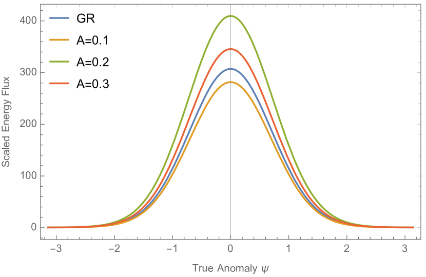
Figure 1: dimensionless instantaneous flux of gravitational energy as function of true anomaly $\psi$ for different values of $A$. It is clear the strong dependence on the non-local parameter $A$: when $A<1/6$ the flux is weaker than the GR equivalent, but it increases as $A$ decreases; when $A>1/6$ the flux is stronger than the GR equivalent, but it decreases as $A$ increases. The most probable range for $A$, i.e. the range of values that deviate the least from the GR prediction, is $A\ll 1$, as expected. An eccentricity value $e=0.5$ has been set.

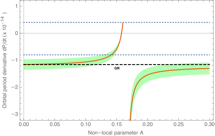
Figure 2: Plot of $\dot{T}$ as a function of $A$ for PSR J$1012+5307$. The range of the observed value ($\dot{P}_{b}^{corr}$) is between the two blue dotted lines: if the theoretical prediction crosses this region then the theory is admissible. While the GR line (dotted black) lies largely outside the region (even considering the error bands), the non-local prediction (orange line) with the corresponding error band (green shading) crosses the strip with non-zero $A$ values. Notice that when $A=0$ the non-local curve reaches the GR prediction, as expected and that the feasible range for $A$ seems to be approximately $0.12<A<0.16$.

5 Summary and conclusions

The use of binary pulsars was the first and most widely used system for testing both GR and modified theories of gravity. Although in the literature the binary system most used as an instrument is PSR $1913+16$, this source is not suitable for such a purpose if only one post-keplerian parameter is studied. Indeed, in this case, one is tempted to use the mass values reported in literature, forgetting that to obtain those values other post-Keplerian parameters were used, usually with the GR assumed to be true (Taylor and Weisberg, 1989). This mixture of underlying theories cannot be useful for making predictions about the theory under study. Therefore, wanting to use the variation of the orbital period to set constraints on alternative theories of gravity, one would have to look for estimates of the masses in an independent way. This is a very crucial point, almost never underlined in the literature. One way to get such masses is to use two additional post-keplerian parameters (such as $\dot{w}$ and $\gamma$), obtained in the specific gravity theory. In our case, they would depend on the non-local parameter $A$, just like $\dot{T}$. However, this approach could be very hard-working and nullified by the fact that post-keplerian parameters different from $\dot{T}$ are not measured with great accuracy. An alternative strategy, in our opinion, could be offered by pulsar-white dwarf binary systems, as in some of these systems the mass of the companion star is obtained from optical observations. From the measurement of the radial velocities of the two bodies, the mass ratio $q=m_{p}/m_{c}$ is also estimated, thus allowing measurements to be obtained for both masses, without ever exploiting timing measurements.

In this paper we followed the second approach, choosing a single post-Keplerian parameter (the variation of the orbital period, $\dot{P}_{b}$) and therefore using three binary pulsars having a white-dwarf as companion star, with all masses obtained spectroscopically or astronometrically. All data are listed in Tables 1 and 2. We computed the total emitted power (or luminosity) as a function of the true anomaly and the theoretical prediction for orbital period variation, $\dot{T}$, emphasizing the non-local contribution. We found that the instantaneous flux of gravitational energy strongly depends on the non-local parameter $A$: when $A<1/6$ the flux is weaker than the GR equivalent, but it increases as $A$ decreases; when $A>1/6$ the flux is stronger than the GR equivalent, but it decreases as $A$ increases. Therefore, based on this, the most probable range for $A$, i.e. the range of values that deviate the least from the GR prediction, is $A\ll 1$, as expected. On the other hand, we compared our prediction, $\dot{T}$, with $\dot{P}_{b}^{corr}$, a corrected version of $\dot{P}_{b}$ (kinematic bias) and we found that, in the case of PSR J$1012+5307$, GR fails to explain the observed values, while an additional non-local contribution could explain them, provided that $0.12<A<0.16$. This means that such a gravity theory should be further investigated. However, it must be said that the inaccuracies on masses and distances are notable, and vary greatly in the literature. Moreover, since for PSR J$1012+5307$ scintillation, i.e. enhanced pulse intensity variations with relatively short timescales and narrow frequency bandwidths, is suspected, as emerged in a recent census by LOFAR (Wu et al., 2022), corruptions in pulsar timing, due to the interstellar medium, could be hidden. This could be a possible explanation for the GR disagreement. Therefore, only by using more precise data and a statistically larger number of sources of this type could confirm, modify or exclude the constraints we found.

Declaration of competing interest

The author declare that they have no known competing financial interests or personal relationships that could have appeared to influence the work reported in this paper.

Data availability

No data was used for the research described in the article.

References

- Amendola et al. (2019) Amendola, L., Dirian, Y., Nersisyan, H., Park, S., 2019. Observational constraints in nonlocal gravity: the deser-woodard case. Journal of Cosmology and Astroparticle Physics 2019, 045–045. URL: https://doi.org/10.1088%2F1475-7516%2F2019%2F03%2F045, doi:10.1088/1475-7516/2019/03/045.
- Antoniadis et al. (2013) Antoniadis, J., Freire, P.C.C., Wex, N., Tauris, T.M., Lynch, R.S., van Kerkwijk, M.H., Kramer, M., Bassa, C., Dhillon, V.S., Driebe, T., Hessels, J.W.T., Kaspi, V.M., Kondratiev, V.I., Langer, N., Marsh, T.R., McLaughlin, M.A., Pennucci, T.T., Ransom, S.M., Stairs, I.H., van Leeuwen, J., Verbiest, J.P.W., Whelan, D.G., 2013. A massive pulsar in a compact relativistic binary. Science 340. URL: https://doi.org/10.1126%2Fscience.1233232, doi:10.1126/science.1233232.
- Bahamonde et al. (2017) Bahamonde, S., Capozziello, S., Faizal, M., Nunes, R.C., 2017. Nonlocal Teleparallel Cosmology. Eur. Phys. J. C 77, 628. doi:10.1140/epjc/s10052-017-5210-1, arXiv:1709.02692.
- Biswas et al. (2012) Biswas, T., Gerwick, E., Koivisto, T., Mazumdar, A., 2012. Towards singularity- and ghost-free theories of gravity. Physical Review Letters 108. URL: https://doi.org/10.1103%2Fphysrevlett.108.031101, doi:10.1103/physrevlett.108.031101.
- Buoninfante et al. (2018) Buoninfante, L., Koshelev, A.S., Lambiase, G., Mazumdar, A., 2018. Classical properties of non-local, ghost- and singularity-free gravity. Journal of Cosmology and Astroparticle Physics 2018, 034–034. URL: https://doi.org/10.1088%2F1475-7516%2F2018%2F09%2F034, doi:10.1088/1475-7516/2018/09/034.
- Buoninfante et al. (2020) Buoninfante, L., Lambiase, G., Miyashita, Y., Takebe, W., Yamaguchi, M., 2020. Generalized ghost-free propagators in nonlocal field theories. Physical Review D 101. URL: https://doi.org/10.1103%2Fphysrevd.101.084019, doi:10.1103/physrevd.101.084019.
- Capozziello and Bajardi (2021) Capozziello, S., Bajardi, F., 2021. Nonlocal gravity cosmology: An overview. International Journal of Modern Physics D 31. URL: https://doi.org/10.1142%2Fs0218271822300099, doi:10.1142/s0218271822300099.
- Capozziello and Capriolo (2021) Capozziello, S., Capriolo, M., 2021. Gravitational waves in non-local gravity. Classical and Quantum Gravity 38, 175008. URL: https://doi.org/10.1088%2F1361-6382%2Fac1720, doi:10.1088/1361-6382/ac1720.
- Capozziello et al. (2020) Capozziello, S., Capriolo, M., Nojiri, S., 2020. Considerations on gravitational waves in higher-order local and non-local gravity. Phys. Lett. B 810, 135821. doi:10.1016/j.physletb.2020.135821, arXiv:2009.12777.
- Capriolo (2022) Capriolo, M., 2022. Gravitational radiation in higher order non-local gravity. International Journal of Geometric Methods in Modern Physics 19. URL: https://doi.org/10.1142%2Fs0219887822501596, doi:10.1142/s0219887822501596.
- Deser and Woodard (2007) Deser, S., Woodard, R.P., 2007. Nonlocal cosmology. Phys. Rev. Lett. 99, 111301. URL: https://link.aps.org/doi/10.1103/PhysRevLett.99.111301, doi:10.1103/PhysRevLett.99.111301.
- Desvignes and et al. (2016) Desvignes, G., et al., 2016. High-precision timing of 42 millisecond pulsars with the european pulsar timing array. Monthly Notices of the Royal Astronomical Society 458, 3341–3380. URL: https://doi.org/10.1093%2Fmnras%2Fstw483, doi:10.1093/mnras/stw483.
- Dialektopoulos et al. (2019) Dialektopoulos, K., Borka, D., Capozziello, S., Jovanović, V.B., Jovanović, P., 2019. Constraining nonlocal gravity by s2 star orbits. Physical Review D 99. URL: https://doi.org/10.1103%2Fphysrevd.99.044053, doi:10.1103/physrevd.99.044053.
- Ding et al. (2020) Ding, H., Deller, A.T., Freire, P., Kaplan, D.L., Lazio, T.J.W., Shannon, R., Stappers, B., 2020. Very long baseline astrometry of PSR j1012+5307 and its implications on alternative theories of gravity. The Astrophysical Journal 896, 85. URL: https://doi.org/10.3847%2F1538-4357%2Fab8f27, doi:10.3847/1538-4357/ab8f27.
- Edholm (2018) Edholm, J., 2018. Gravitational radiation in infinite derivative gravity and connections to effective quantum gravity. Physical Review D 98. URL: https://doi.org/10.1103%2Fphysrevd.98.044049, doi:10.1103/physrevd.98.044049.
- Edholm (2019) Edholm, J., 2019. Infinite derivative gravity: A finite number of predictions. arXiv:1904.10248.
- Efimov (1967) Efimov, G.V., 1967. Non-local quantum theory of the scalar field. Commun. Math. Phys. 5, 42–56. doi:10.1007/BF01646357.
- Efimov (1968) Efimov, G.V., 1968. On a class of relativistic invariant distributions. Commun. Math. Phys. 7, 138–151. doi:10.1007/BF01648331.
- Efimov (1974) Efimov, G.V., 1974. Quantization of non-local field theory. Int. J. Theor. Phys. 10, 19–37. doi:10.1007/BF01808314.
- Efimov et al. (1977) Efimov, G.V., Ivanov, M.A., Mogilevsky, O.A., 1977. Electron self-energy in nonlocal field theory. Annals Phys. 103, 169–184. doi:10.1016/0003-4916(77)90267-6.
- Efimov and Mogilevsky (1972) Efimov, G.V., Mogilevsky, O.A., 1972. On the choice of form factors in non-local quantum electrodynamics. Nucl. Phys. B 44, 541–557. doi:10.1016/0550-3213(72)90136-8.
- Eliezer and Woodard (1989) Eliezer, D.A., Woodard, R.P., 1989. The Problem of Nonlocality in String Theory. Nucl. Phys. B 325, 389. doi:10.1016/0550-3213(89)90461-6.
- Freire et al. (2012a) Freire, P.C.C., Wex, N., Esposito-Farè se, G., Verbiest, J.P.W., Bailes, M., Jacoby, B.A., Kramer, M., Stairs, I.H., Antoniadis, J., Janssen, G.H., 2012a. The relativistic pulsar-white dwarf binary PSR j17380333 - II. the most stringent test of scalar-tensor gravity. Monthly Notices of the Royal Astronomical Society 423, 3328–3343. URL: https://doi.org/10.1111%2Fj.1365-2966.2012.21253.x, doi:10.1111/j.1365-2966.2012.21253.x.
- Freire et al. (2012b) Freire, P.C.C., Wex, N., Esposito-Farè se, G., Verbiest, J.P.W., Bailes, M., Jacoby, B.A., Kramer, M., Stairs, I.H., Antoniadis, J., Janssen, G.H., 2012b. The relativistic pulsar-white dwarf binary PSR j1738+0333 - II. the most stringent test of scalar-tensor gravity. Monthly Notices of the Royal Astronomical Society 423, 3328–3343. URL: https://doi.org/10.1111%2Fj.1365-2966.2012.21253.x, doi:10.1111/j.1365-2966.2012.21253.x.
- Kapner et al. (2007) Kapner, D.J., Cook, T.S., Adelberger, E.G., Gundlach, J.H., Heckel, B.R., Hoyle, C.D., Swanson, H.E., 2007. Tests of the gravitational inverse-square law below the dark-energy length scale. Phys. Rev. Lett. 98, 021101. doi:10.1103/PhysRevLett.98.021101, arXiv:hep-ph/0611184.
- Laurentis and Capozziello (2011) Laurentis, M.D., Capozziello, S., 2011. Quadrupolar gravitational radiation as a test-bed for f(r)-gravity. Astroparticle Physics 35, 257–265. URL: https://doi.org/10.1016%2Fj.astropartphys.2011.08.006, doi:10.1016/j.astropartphys.2011.08.006.
- Laurentis and Martino (2013) Laurentis, M.D., Martino, I.D., 2013. Testing f (r) theories using the first time derivative of the orbital period of the binary pulsars. Monthly Notices of the Royal Astronomical Society 431, 741–748. URL: https://doi.org/10.1093%2Fmnras%2Fstt216, doi:10.1093/mnras/stt216.
- Laurentis and Martino (2015) Laurentis, M.D., Martino, I.D., 2015. Probing the physical and mathematical structure of f(r)-gravity by PSR j0348 + 0432. International Journal of Geometric Methods in Modern Physics 12, 1550040. URL: https://doi.org/10.1142%2Fs0219887815500401, doi:10.1142/s0219887815500401.
- Maggiore (2007) Maggiore, M., 2007. Gravitational Waves. Vol. 1: Theory and Experiments. Oxford University Press. doi:10.1093/acprof:oso/9780198570745.001.0001.
- Mashhoon (2022) Mashhoon, B., 2022. Nonlocal Gravity: Fundamental Tetrads and Constitutive Relations. Symmetry 14, 2116. doi:10.3390/sym14102116, arXiv:2209.05817.
- Modesto (2012) Modesto, L., 2012. Super-renormalizable quantum gravity. Physical Review D 86. URL: https://doi.org/10.1103%2Fphysrevd.86.044005, doi:10.1103/physrevd.86.044005.
- Modesto et al. (2011) Modesto, L., Moffat, J.W., Nicolini, P., 2011. Black holes in an ultraviolet complete quantum gravity. Physics Letters B 695, 397–400. URL: https://doi.org/10.1016%2Fj.physletb.2010.11.046, doi:10.1016/j.physletb.2010.11.046.
- Modesto and Rachwał (2015) Modesto, L., Rachwał, L., 2015. Universally finite gravitational and gauge theories. Nucl. Phys. B 900, 147–169. doi:10.1016/j.nuclphysb.2015.09.006, arXiv:1503.00261.
- Modesto and Shapiro (2016) Modesto, L., Shapiro, I.L., 2016. Superrenormalizable quantum gravity with complex ghosts. Phys. Lett. B 755, 279–284. doi:10.1016/j.physletb.2016.02.021, arXiv:1512.07600.
- Nazari et al. (2022) Nazari, E., Roshan, M., Martino, I.D., 2022. Constraining energy-momentum-squared gravity by binary pulsar observations. Physical Review D 105. URL: https://doi.org/10.1103%2Fphysrevd.105.044014, doi:10.1103/physrevd.105.044014.
- Pauli (1953) Pauli, W., 1953. On the Hamiltonian structure of non-local field theories. Nuovo Cim. 10, 648–667. doi:10.1007/bf02815288.
- Pauli and Villars (1949) Pauli, W., Villars, F., 1949. On the Invariant regularization in relativistic quantum theory. Rev. Mod. Phys. 21, 434–444. doi:10.1103/RevModPhys.21.434.
- Prager et al. (2017) Prager, B.J., Ransom, S.M., Freire, P.C.C., Hessels, J.W.T., Stairs, I.H., Arras, P., Cadelano, M., 2017. Using long-term millisecond pulsar timing to obtain physical characteristics of the bulge globular cluster terzan 5. The Astrophysical Journal 845, 148. URL: https://doi.org/10.3847%2F1538-4357%2Faa7ed7, doi:10.3847/1538-4357/aa7ed7.
- Puetzfeld et al. (2019) Puetzfeld, D., Obukhov, Y.N., Hehl, F.W., 2019. Constitutive law of nonlocal gravity. Physical Review D 99. URL: https://doi.org/10.1103%2Fphysrevd.99.104013, doi:10.1103/physrevd.99.104013.
- Sanchez et al. (2020) Sanchez, D.M., Istrate, A.G., van Kerkwijk, M.H., Breton, R.P., Kaplan, D.L., 2020. PSR j1012+5307: a millisecond pulsar with an extremely low-mass white dwarf companion. Monthly Notices of the Royal Astronomical Society 494, 4031–4042. URL: https://doi.org/10.1093%2Fmnras%2Fstaa983, doi:10.1093/mnras/staa983.
- Shklovskii (1970) Shklovskii, I.S., 1970. Possible Causes of the Secular Increase in Pulsar Periods. Soviet Astronomy 13, 562.
- Siegel (2003) Siegel, W., 2003. Stringy gravity at short distances. arXiv:hep-th/0309093.
- Stairs (2003) Stairs, I.H., 2003. Testing general relativity with pulsar timing. Living Reviews in Relativity 6. URL: https://doi.org/10.12942%2Flrr-2003-5, doi:10.12942/lrr-2003-5.
- Taylor and Weisberg (1989) Taylor, J.H., Weisberg, J.M., 1989. Further Experimental Tests of Relativistic Gravity Using the Binary Pulsar PSR 1913+16. Apj 345, 434. doi:10.1086/167917.
- Wu et al. (2022) Wu, Z., Verbiest, J.P.W., Main, R.A., Grießmeier, J.M., Liu, Y., Osłowski, S., Moochickal Ambalappat, K., Nielsen, A.S.B., Künsemöller, J., Donner, J.Y., Tiburzi, C., Porayko, N., Serylak, M., Künkel, L., Brüggen, M., Vocks, C., 2022. Pulsar scintillation studies with LOFAR. I. The census. AAP 663, A116. doi:10.1051/0004-6361/202142980, arXiv:2203.10409.