Spectral Deconfounding for High-Dimensional Sparse Additive Models

Abstract

Many high-dimensional data sets suffer from hidden confounding. When hidden confounders affect both the predictors and the response in a high-dimensional regression problem, standard methods lead to biased estimates. This paper substantially extends previous work on spectral deconfounding for high-dimensional linear models to the nonlinear setting and with this, establishes a proof of concept that spectral deconfounding is valid for general nonlinear models. Concretely, we propose an algorithm to estimate high-dimensional additive models in the presence of hidden dense confounding: arguably, this is a simple yet practically useful nonlinear scope. We prove consistency and convergence rates for our method and evaluate it on synthetic data and a genetic data set.

1 Introduction

We consider estimation of nonlinear additive functions in the presence of dense unobserved confounding in the high-dimensional and sparse setting. Unobserved confounding is a severe problem in practice leading to large and asymptotically non-vanishing bias. While some progress on deconfounding and removing of bias has been achieved in the context of observational data from linear models, the current paper establishes the theory and methodology for nonlinear additive models with dense confounding. In particular, we build on spectral deconfounding introduced in [8] which is simple and often more accurate than inferring hidden factor variables and then adjusting for them. The development of spectral deconfounding for nonlinear problems is new and requires careful theoretical analysis: yet, we believe it is important as it opens a path for addressing unobserved confounding in the context of nonlinear, high-dimensional regression.

We focus in this paper on estimation, based on observational data, of high-dimensional sparse additive models in the presence of hidden confounding. More concretely, we look at the following model

$$Y=f^{0}(X)+H^{T}\psi+e\quad\text{and}\quad X=\Psi^{T}H+E,$$ (1)

where $Y\in\mathbb{R}$ denotes the outcome variable, $X\in\mathbb{R}^{p}$ denotes the high-dimensional covariates, $H\in\mathbb{R}^{q}$ denotes the hidden confounders, $e\in\mathbb{R}$ and $E\in\mathbb{R}^{p}$ stand for random noises, and $f^{0}(X)=\beta_{0}^{0}+\sum_{j\in\mathcal{T}}f_{j}^{0}(X_{j})$ is an unknown sparse additive function with active set $\mathcal{T}\subset\{1,\ldots,p\}$ and $|\mathcal{T}|\ll p$. We assume that $H$ is low-dimensional ($q\ll p$) and that the confounding is dense (i.e. $H$ affects many components of $X$). The goal is to accurately estimate $f^{0}$ and the individual additive functions $f_{j}^{0}$. Note that a naive (nonlinear) regression of $Y$ on $X$ yields an estimate of $\mathbb{E}[Y|X]=f^{0}(X)+\mathbb{E}[H|X]^{T}\psi$ (assuming $\mathbb{E}[e|X]=0$). Hence an estimate of $f^{0}$ obtained in this naive way is biased. If the goal merely is prediction in the setting of model (1), such a biased estimate may still appear useful at first sight. However, as argued in [7] for the linear case, estimating the function $f^{0}$ instead is desirable from the viewpoint of stability and replicability. For example, the effect of the confounder $H$ might be different for new data from an other environment, such that an estimator of the form $\mathbb{E}[Y|X]$ fails to yield a reliable prediction. Moreover, if the confounding acts densely on $X$, $\mathbb{E}[Y|X]$ will not be sparse and algorithms tailored for sparsity will be the wrong choice. If one interprets (1) as a structural equations model (SEM), one can view $f^{0}$ as the direct causal effect of $X$ on $Y$ where the variables $X_{\mathcal{T}}$ are the causal parents of $Y$.

1.1 Spectral Transformations for Deconfounding: Easy Implementation and Robustness against Dense Confounding

Spectral transformations for deconfounding have been introduced for high-dimensional sparse linear models in [8]. They provide a class of linear transformation matrices: denoting a member of this class by $Q$, one simply applies $Q$ to the data and then proceeds as usual, e.g. with Lasso for high-dimensional linear models. Constructing such a $Q$ is extremely simple: one just needs the singular values decomposition of the $n\times p$ design matrix $\mathbf{X}$. In its default version with the so-called trim transformation, one does not need to specify a tuning parameter such as the dimensionality $q$ of $H$ or an upper bound of it.

Spectral transformations have been shown to adjust (and remove) the effect of the hidden confounder $H$, under the assumption that $H$ acts densely on $X$, that is, many components of $X$ are affected by $H$. In such a scenario, one could alternatively estimate the matrix $\mathbf{H}\in\mathbb{R}^{n\times q}$ (with $n$ i.i.d. unobserved samples of $H$ as rows) by principal components of $\mathbf{X}$, say $\hat{\mathbf{H}}$, and then adjust with $\hat{\mathbf{H}}$. Such methodology and theory relies on fundamental results about high-dimensional latent factor models, see for example the review by [1]. However, with such an approach, one needs to estimate an upper bound of the latent factor dimension $q$, and that itself is known to be a difficult task, see for example the discussion in [28]. For estimating the unconfounded regression parameter or function though, one does not necessarily need to have an accurate estimate of $\mathbf{H}$: spectral transformations avoid selecting an upper bound of $q$ and they also work under weaker assumptions than relying on approximate recovery of $\mathbf{H}$, see [19]. Spectral transformations and corresponding deconfounding has been demonstrated to work very well in practice and theory in high-dimensional linear models with dense confounding [8, 19]. Even when the models are mis-specified to a certain extent or when assumptions do not completely hold, extensive simulations have shown some robustness against dense (or at least fairly dense) confounding.

These substantial practical, empirical and theoretical advantages of spectral transformations for deconfounding remained unclear for nonlinear models. We establish here that the good properties of spectral transformations carry over to nonlinear additive models. The theoretical derivations are highly non-trivial, essentially because spectral transformations are based on $X$ but then applied to nonlinear (basis) functions $b_{j}(X_{j})=b_{j}(\Psi_{j}^{T}H+E_{j})$, where the hidden confounder $H$ is now in the argument of a nonlinear function $b_{j}(\cdot)$ but spectral deconfounding (and also PCA) are intrinsically based on linear operations.

1.2 Motivating Example

We consider a motivating example. We fix $n=300$, $p=800$ and $q=5$ and simulate from model (1) for a nonlinear additive function $f^{0}(X)=\sum_{j\in\mathcal{T}}f_{j}^{0}(X_{j})$ with $\mathcal{T}=\{1,2,3,4\}$. We refer to Section 4.2 for the exact specification of the simulation scenario. We simulate 100 data sets and fit a high-dimensional additive model on each data set without deconfounding (“naive”) and with our deconfounded method (“deconfounded”). Histograms of the mean squared errors $\|\hat{f}-f^{0}\|_{L_{2}}^{2}$ and the size of the estimated active set are provided in Figure 1.

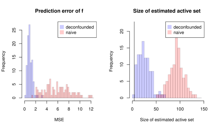
Figure 1: MSE of estimated function for true $f^{0}$ (left) and size of estimated active set (right) for our proposed method (“deconfounded”) and the standard high-dimensional additive model fitting procedure (“naive”). The vertical bar in the right plot indicates the true size of the active set, which is $4$.

We see that our method clearly outperforms the standard “naive” approach both in terms of estimation error and also in terms of variable screening as the size of the estimated active set is much smaller, though both methods significantly over-estimate the size of the active set. A more detailed simulation study with discussion can be found in Section 4.

1.3 Related Work

Our work is most related to the literature on spectral deconfounding, introduced in [8]. In the case of dense confounding, they use a spectral transformation which is applied to the data and use the lasso for the transformed data to get a consistent estimator of the coefficient vector in high-dimensional linear regression. This turns out to be related to the Lava method for linear regression [9] where the coefficient vector can be written as the sum of a sparse and a dense part. As an extension of spectral deconfounding, a doubly debiased lasso estimator was proposed in [19], which allows to perform inference for individual components of the coefficient vector. The idea of spectral deconfounding has also been applied in [3] to the estimation of sparse linear Gaussian directed acylic graphs in the presence of hidden confounding.

There is an active area of research that considers variants of model (1), mostly in the case where $f^{0}$ is linear, but does not use spectral transformations in the sense of [8]. The following works all have in common that they in some way explicitly estimate the hidden confounders $H$ from $X$ or need to know or estimate the dimension $q$ of $H$ (although, in many cases, the methods can be rewritten using the PCA transformation defined in Appendix B.1). For example, [20, 14, 15] all consider regression problems, where the covariates $X$ come from a high-dimensional factor model. We refer to [8] and [19] for a more detailed discussion of related literature in the case of high-dimensional linear regression. More recently, also simultaneous inference for high-dimensional linear regression [32] as well as estimation and inference for high-dimensional multivariate response regression [5, 4] have been considered in the presence of hidden confounding. There have also been some advances towards nonlinear models using this framework. In [27], a debiased estimator is introduced for the high-dimensional generalized linear model with hidden confounding and consistency and asymptotic normality for the estimator is established. Most recently and perhaps most related to our nonlinear setting, [12] consider a factor model $X=\Psi^{T}H+E$ for the covariates and a response $Y=m^{\ast}(H,E_{\mathcal{J}})+\epsilon_{i}$, where $\mathcal{J}$ is the active set. The goal is to estimate the function $m^{\ast}$, which is done by fitting a neural network. As a special case, this framework also allows to estimate additive models similar to (1). However, the goal of [12] is distinctively different from ours. The main goal of our paper is to consistently estimate the function $f$, which can be interpreted causally. For this, we implicitly filter out the factors using a spectral transformation. The goal of [12] on the other hand, is to estimate the function $m^{\ast}$ which depends on the factors with the reason that including the factors helps to predict $Y$. We defer the discussion of more technical differences to Section 3.4.

Finally, for the case of unconfounded settings, high-dimensional additive models have been extensively studied as a more flexible alternative to the high-dimensional linear model while still avoiding the curse of dimensionality [25, 30, 29, 24, 34, 21, 22].

1.4 Our Contribution and Outline

We propose a novel estimator for high-dimensional additive models in the presence of hidden confounding. For this, we expand the unknown functions $f_{j}$ into basis functions (e.g. B-splines) as done in [25] and apply a spectral transformation as introduced in [8] to the response and to the basis functions. On this transformed data, we apply an ordinary group lasso optimization to obtain the estimates $\hat{f}_{j}$. For this procedure, we prove consistency and provide both in-sample and $L_{2}$ convergence rates. Our method achieves a convergence rate of

$$\|\hat{f}-f^{0}\|_{L_{2}}=O_{P}\left(\frac{s\sqrt{\log p}}{n^{2/5}}+\frac{s^{2}}{n^{2/5}\sqrt{\log p}}\right)$$

for the standard choice of $K\asymp n^{1/5}$ basis functions under suitable assumptions. Our developed theory is novel as it addresses for the first time the problem of spectral deconfounding in the context of nonlinearity in the regression function. The theoretical steps are challenging, particularly in terms of establishing that a group compatibility constant is bounded away from zero (also known as restricted eigenvalue condition). We perform a simulation study to illustrate the effectiveness and apply the method on a genetic data set. In conclusion, our method is much more robust against hidden confounding than standard additive model techniques, even if the model is moderately mis-specified.

The rest of the paper is structured as follows. In Section 2, we introduce our setup and formulate the optimization problem. In Section 3, we prove consistency and convergence rates for our method under suitable assumptions. We first present a general convergence result that holds under minimal assumptions (Theorem 1). This convergence rate depends on unknown parameters, namely a compatibility constant, the effect of the spectral transformation, and the best approximation of $f_{j}^{0}$ using the specified basis functions. These parameters are then subsequently controlled under some stronger assumptions. The experiments on simulated and real data can be found in Section 4. All the proofs are presented in the appendix.

1.5 Notation and Conventions

We write $\lambda_{j}(A)$ for the $j$-th largest singular value of the matrix $A$. If $A$ is symmetric and positive semi-definite, we also writhe $\lambda_{\max}(A)$ and $\lambda_{\min}(A)$ for the maximal and the minimal eigenvalue of $A$. We write $\|A\|_{F}$, $\|A\|_{op}$ and $\|A\|_{\infty}$ for the Frobenius norm, operator/spectral norm and the element-wise maximum norm of the matrix $A$. For a sequence of random variables $X_{n}$ and a sequence of real numbers $a_{n}$, we write $X_{n}=o_{P}(a_{n})$ if $X_{n}/a_{n}\to 0$ in probability and $X_{n}=O_{P}(a_{n})$ if $\lim_{M\to\infty}\limsup_{n\to\infty}\mathbb{P}(|X_{n}|/a_{n}>M)=0$. For two sequences $a_{n}$ and $b_{n}$ of positive real numbers, we write $a_{n}\lesssim b_{n}$ if there exists a constant $C>0$ such that $a_{n}\leq Cb_{n}$ for all $n\in\mathbb{N}$. We write $a_{n}\asymp b_{n}$ if $a_{n}\lesssim b_{n}$ and $b_{n}\lesssim a_{n}$ and $a_{n}\ll b_{n}$ if $\lim_{n\to\infty}a_{n}/b_{n}=0$. For a random variable $X$, $\|X\|_{\psi_{2}}=\inf\{t>0|\mathbb{E}[\exp(X^{2}/t^{2})\leq 2\}$ is the sub-Gaussian norm of $X$. We call $X$ a sub-Gaussian random variable if $\|X\|_{\psi_{2}}<\infty$. For a random vector $Z\in\mathbb{R}^{d}$, let $\|Z\|_{\psi_{2}}=\sup_{\|v\|_{2}=1}\|v^{T}Z\|_{\psi_{2}}$ and we call $Z$ a sub-Gaussian random vector if $\|Z\|_{\psi_{2}}<\infty$. We say that an event $\mathcal{A}$ occurs with high probability if $\mathbb{P}(\mathcal{A})=1-o(1)$ for $n\to\infty$. For a real number $t\in\mathbb{R}$, we write $\lfloor t\rfloor$ for the floor function, i.e. the largest integer smaller or equal to $t$. We write $I_{l}$ for the $l\times l$ identity matrix and $\mathbf{1}_{l}=(1,\ldots,1)^{T}\in\mathbb{R}^{l}$ for the vector of $l$ ones.

2 Model and Method

We consider the model

$$Y=f^{0}(X)+H^{T}\psi+e\quad\text{and}\quad X=\Psi^{T}H+E$$ (2)

with random variables $H\in\mathbb{R}^{q}$, $X\in\mathbb{R}^{p}$ and $Y\in\mathbb{R}$, random errors $e\in\mathbb{R}$ and $E\in\mathbb{R}^{p}$ and fixed $\psi\in\mathbb{R}^{q}$ and $\Psi\in\mathbb{R}^{q\times p}$. We only observe $X$ and $Y$ and the confounder $H$ is unobserved. The goal is to estimate the unknown function $f^{0}$. In this work, we assume an additive and sparse structure of $f^{0}$, i.e.

$$f^{0}(X)=\beta_{0}^{0}+\sum_{j=1}^{p}f_{j}^{0}(X_{j})=\beta_{0}^{0}+\sum_{j\in\mathcal{T}}f_{j}^{0}(X_{j}),$$

with $\mathcal{T}\subset\{1,\ldots,p\}$ and $|\mathcal{T}|=s$ being the active set. For identifiability, we assume that $\mathbb{E}[f_{j}(X_{j})]=0$ for all $j=1,\ldots,p$. To fix some notation, $x_{1},\ldots,x_{n}\in\mathbb{R}^{p}$, $y_{1},\ldots,y_{n}\in\mathbb{R}$ and $h_{1},\ldots,h_{n}\in\mathbb{R}^{q}$ are i.i.d. samples from (2). Let $\mathbf{X}\in\mathbb{R}^{n\times p}$ have rows $x_{1},\ldots,x_{n}$, $\mathbf{Y}\in\mathbb{R}^{n}$ have entries $y_{1},\ldots,y_{n}$ and $\mathbf{H}\in\mathbb{R}^{n\times q}$ have rows $h_{1},\ldots,h_{n}$.

For each $j=1,\ldots,p$, we approximate $f_{j}^{0}$ using a set of basis functions, for example, a B-spline basis. The number of basis functions $K$ serves as a tuning parameter for smoothness. Define $b_{j}(\cdot)=b_{j}^{(n)}(\cdot)=(b_{j}^{1}(\cdot),\ldots,b_{j}^{K}(\cdot))^{T}$ to be the vector of basis functions for the $j$th component of $X$. The general idea of high-dimensional sparse additive models is to regress $Y$ on $(b_{1}(X_{1})^{T},\ldots,b_{p}(X_{p})^{T})^{T}$ using a group lasso scheme. We apply the trim transformation as in [8] to deal with the hidden confounding. Let $r=\min(n,p)$ and $\mathbf{X}\mathbf{X}^{T}=UDU^{T}$ be the eigenvalue decomposition of $\mathbf{X}\mathbf{X}^{T}$ with matrices $U\in\mathbb{R}^{n\times n}$ having orthonormal columns and $D=\operatorname{diag}(d_{1}^{2},\ldots,d_{r}^{2},0,\ldots,0)$ with $d_{1}\geq\ldots\geq d_{r}>0$ being the nonzero singular values of $\mathbf{X}$. Define for $l=1,\ldots,r$, $\tilde{d}_{l}=\min(d_{\lfloor\rho r\rfloor}/d_{l},1)$ for some $\rho\in(0,1)$ and define

$$Q=Q^{\text{trim}}=U\operatorname{diag}(\tilde{d}_{1},\ldots,\tilde{d}_{r},1,\ldots,1)U^{T}.$$ (3)

Usually, one takes $\rho=0.5$, that is $Q$ shrinks the top half of the singular values of $\mathbf{X}$ to the median singular value of $\mathbf{X}$.

For $j=1,\ldots,p$, define the matrix

$$B^{(j)}=B^{(j)}(\mathbf{X}_{\cdot j})=\begin{pmatrix}b_{j}^{1}(x_{1,j})&\cdots&b_{j}^{K}(x_{1,j})\\ \vdots&\ddots&\vdots\\ b_{j}^{1}(x_{n,j})&\cdots&b_{j}^{K}(x_{n,j})\end{pmatrix}\in\mathbb{R}^{n\times K}.$$

Let $\mathbf{1}_{n}=(1,\ldots,1)^{T}\in\mathbb{R}^{n}$. We propose the group lasso estimator

$$\hat{\beta}=\arg\min_{\beta=(\beta_{0},\beta_{1}^{T},\ldots,\beta_{p}^{T})^{T}\in\mathbb{R}^{Kp+1}}\left\{\frac{1}{n}\left\|Q(\mathbf{Y}-\beta_{0}\mathbf{1}_{n}-\sum_{j=1}^{p}B^{(j)}\beta_{j})\right\|_{2}^{2}+\frac{\lambda}{\sqrt{n}}\sum_{j=1}^{p}\left\|B^{(j)}\beta_{j}\right\|_{2}\right\},$$ (4)

and construct the estimators $\hat{f}_{j}(\cdot)=b_{j}(\cdot)^{T}\hat{\beta}_{j}$ and $\hat{f}(X)=\hat{\beta}_{0}+\sum_{j=1}^{p}\hat{f}_{j}(X_{j})$. In the optimization problem (4), $\lambda$ serves as a tuning parameter for sparsity and $K$ as a tuning parameter for smoothness. Note that the matrices $B^{(j)}$ depend on $K$. Our method is summarized in Algorithm 1. Observe that we use the transformation $\tilde{B}^{(j)}=B^{(j)}R_{j}^{-1}$ and $\tilde{\beta}_{j}=R_{j}\beta_{j}$ with $R_{j}^{T}R_{j}=\frac{1}{n}(B^{(j)})^{T}B^{(j)}$ to transform (4) to an ordinary group lasso problem [35] with the penalty $\lambda\sum_{j=1}^{p}\|\tilde{\beta}_{j}\|_{2}$.

Algorithm 1 Deconfounding for high-dimensional additive models

Input: Data $\mathbf{X}\in\mathbb{R}^{n\times p}$, $\mathbf{Y}\in\mathbb{R}^{n}$, spectral transformation $Q\in\mathbb{R}^{n\times n}$, tuning parameters $\lambda$ and $K$, vectors $b_{j}(\cdot)$ of $K$ basis functions, $j=1,\ldots,p$.

Output: Intercept $\hat{\beta}_{0}$ and functions $\hat{f}_{j}(\cdot)$, $j=1,\ldots,p$.

$B^{(j)}\leftarrow(b_{j}(x_{1,j}),\ldots,b_{j}(x_{n,j}))^{T}\in\mathbb{R}^{n\times K}$

Find $R_{j}\in\mathbb{R}^{K\times K}$ such that $R_{j}^{T}R_{j}=\frac{1}{n}(B^{(j)})^{T}B^{(j)}$ $\triangleright$ Cholesky decomposition

$\tilde{B}^{(j)}\leftarrow B^{(j)}R_{j}^{-1}$

$(\hat{\beta}_{0},\hat{\tilde{\beta}}_{1},\ldots,\hat{\tilde{\beta}}_{p})=\arg\min\{\|Q(\mathbf{Y}-\beta_{0}\mathbf{1}_{n}-\sum_{j=1}^{p}\tilde{B}^{(j)}\tilde{\beta}_{j})\|_{2}^{2}/n+\lambda\sum_{j=1}^{p}\|\tilde{\beta}_{j}\|_{2}\}$ $\triangleright$ Group lasso

$\hat{\beta}_{j}\leftarrow R_{j}^{-1}\hat{\tilde{\beta}}_{j}$, $j=1,\ldots,p$

$\hat{f}_{j}(\cdot)\leftarrow b_{j}(\cdot)^{T}\hat{\beta}_{j}$

The estimator (4) is similar to [25] with the difference that we apply the spectral transformation to the first part of the objective and that we do not have an additional smoothness penalty term but regularize smoothness by the number of basis functions $K$.

2.1 Some Intuition

The intuition for the spectral deconfounding method (4) is analogous to the linear case in [8] and [19]. Let $b\in\mathbb{R}^{p}$ be defined as

$$b=\mathbb{E}[XX^{T}]^{-1}\Psi^{T}\psi,$$ (5)

i.e. $X^{T}b$ is the best linear approximation of $H^{T}\psi$ by $X$ in the sense that $b=\arg\min_{b^{\prime}}\mathbb{E}[(H^{T}\psi-X^{T}b^{\prime})^{2}]$. We can rewrite our model (2) as

$$Y=f^{0}(X)+X^{T}b+\epsilon,\quad\epsilon=e+H^{T}\psi-X^{T}b.$$ (6)

The heuristics is that – in contrast to $\frac{1}{\sqrt{n}}\|\mathbf{X}b\|_{2}$ which is large due to the factor structure and large singular values of $\mathbf{X}$ – the quantity $\frac{1}{\sqrt{n}}\|Q\mathbf{X}b\|_{2}$ converges to $0$ (see Lemma 8 below). If on the other hand, $Q$ does not shrink the vector $\mathbf{f}^{0}=(f^{0}(x_{1}),\ldots,f^{0}(x_{n}))^{T}\in\mathbb{R}^{n}$ too much, it seems reasonable that an $\hat{f}$ obtained by minimizing $\|Q\mathbf{Y}-Q\mathbf{f}\|_{2}$ should recover $f^{0}$ much better than an $\hat{f}$ obtained by minimizing $\|\mathbf{Y}-\mathbf{f}\|_{2}$.

3 Theory

In this section, we develop and describe the key mathematical results of the proposed procedure in Algorithm 1, and we give conditions under which our method is consistent and give rates for the convergence of $\hat{f}$ to $f$. We will show in Corollary 9 that under suitable assumptions and with the standard choices of $\lambda\asymp\sqrt{\log(p)/n^{4/5}}$ and $K\asymp n^{1/5}$, we obtain a rate of

$$|\beta_{0}^{0}-\hat{\beta}_{0}|+\sum_{j=1}^{p}\|f_{j}^{0}-\hat{f}_{j}\|_{L_{2}}=O_{P}\left(\frac{s}{n^{2/5}}\sqrt{\log p}+\frac{s^{2}}{n^{2/5}\sqrt{\log p}}\right).$$ (7)

If instead, we optimize $K$ depending on $n$, $p$, and $s$, we obtain a convergence rate of $O_{P}\left(s^{11/10}\frac{(\log p)^{2/5}}{n^{2/5}}\right)$. However, our main results Theorem 1 and Corollary 3 hold under much more general conditions. The general convergence rate (11) in these results depends on several general quantities like a compatibility constant and on how well the functions $f_{j}^{0}$ can be approximated by the basis functions $b_{j}(\cdot)$. These quantities are then subsequently controlled under stronger assumptions to arrive at the convergence rate given above.

We start with the following assumptions on the model (2).

Assumption 1.

1. The random vectors $H$ and $E$ are centered, i.e. $\mathbb{E}[H]=0\in\mathbb{R}^{q}$, $\mathbb{E}[E]=0\in\mathbb{R}^{p}$, and the entries of $E$ and $H$ have finite second moment. Moreover, $\mathbb{E}[EH^{T}]=0\in\mathbb{R}^{p\times q}$ and $\mathbb{E}[HH^{T}]=I_{q}$.

2. The random variable $e$ is independent of $(H,E)$ and has sub-Gaussian distribution with $\mathbb{E}[e]=0$, $\mathbb{E}[e^{2}]=\sigma_{e}^{2}$ and $\|e\|_{\psi_{2}}\leq C_{0}$.

3. $q\ll\min(n,p)$.

The assumption $\mathbb{E}[EH^{T}]=0$ means that the random vectors $E$ and $H$ are uncorrelated. The assumption that $\mathbb{E}[HH^{T}]=I_{q}$ can be made without loss of generality. If $\mathbb{E}[HH^{T}]=\Sigma_{H}$, define $\tilde{H}=\Sigma_{H}^{-1/2}H$, $\tilde{\Psi}=\Sigma_{H}^{1/2}\Psi$ and $\tilde{\psi}=\Sigma_{H}^{1/2}\psi$. Then, $\mathbb{E}[\tilde{H}\tilde{H}^{T}]=I_{q}$ and we are again in the framework of model (2).

For Theorem 1 below, we need the following additional assumption.

Assumption 2.

Let $\Sigma_{E}=\mathbb{E}[EE^{T}]$. There exist $C,c>0$ such that $c\leq\lambda_{\min}(\Sigma_{E}^{-1})\leq\lambda_{\max}(\Sigma_{E}^{-1})\leq C$.

Note that we only need a bound for the minimal eigenvalue of the precision matrix of the unconfounded part $E$ and not of $X$. This is crucial since because of the factor structure, the precision matrix of $X$ would not be nicely behaved.

For $j=1,\ldots,p$, let $f_{j}^{\ast}$ be an approximation of $f_{j}^{0}$ using the $K$ basis functions in $b_{j}(\cdot)$, that is

$$f_{j}^{\ast}(\cdot)=b_{j}(\cdot)^{T}\beta_{j}^{\ast},$$

and let $f^{\ast}(X)=\beta_{0}^{0}+\sum_{j=1}^{p}f_{j}^{\ast}(X_{j})$. Define the vectors $\mathbf{f}_{j}^{0}=(f_{j}^{0}(x_{1,j}),\ldots,f_{j}^{0}(x_{n,j}))^{T}\in\mathbb{R}^{n}$ and $\mathbf{f}^{0}=(f^{0}(x_{1}),\ldots,f^{0}(x_{n}))^{T}\in\mathbb{R}^{n}$ and similarly also $\hat{\mathbf{f}}_{j}$, $\hat{\mathbf{f}}$, $\mathbf{f}_{j}^{\ast}$ and $\mathbf{f}^{\ast}$.

For technical reasons, we also need the following assumption on the basis functions, which is for example fulfilled for the B-spline basis (see Chapter 8 in [11]).

Assumption 3 (Partition of unity).

For all $j=1,\ldots,p$ and for all $x\in\textup{support}(X_{j})$, we have that $b_{j}(x)^{T}\mathbf{1}_{K}=1$.

We furthermore need to define the sample compatibility constant. For $w_{0}\in\mathbb{R}$ and $w_{j}\in\mathbb{R}^{K}$, $j=1,\ldots,p$, let us write $f_{j}^{w}(\cdot)=b_{j}(\cdot)^{T}w_{j}$ and $f^{w}(x)=w_{0}+\sum_{j=1}^{p}f_{j}^{w}(x_{j})$. Moreover, for $M>0$ and $\mathcal{T}\subset\{1,\ldots,p\}$ define,

$$\mathcal{F}_{M,\mathcal{T}}^{n}=\left\{f^{w}:w_{0}\in\mathbb{R},w_{j}\in\mathbb{R}^{K},\,\sum_{i=1}^{n}f_{j}^{w}(x_{i,j})=0\text{ and }\sum_{j\in\mathcal{T}^{c}}\frac{1}{\sqrt{n}}\|\mathbf{f}_{j}^{w}\|_{2}\leq M\left(|w_{0}|+\sum_{j\in\mathcal{T}}\frac{1}{\sqrt{n}}\|\mathbf{f}_{j}^{w}\|_{2}\right)\right\}.$$ (8)

Note that the functions $f_{j}^{w}$ defining the functions $f^{w}$ in $\mathcal{F}_{M,\mathcal{T}}^{n}$ are empirically centered. We define the sample compatibility constant

$$\tau_{n}=\inf_{\mathcal{T}\subset[p],\,|\mathcal{T}|\leq s}\inf_{f\in\mathcal{F}_{M,\mathcal{T}}^{n}}\frac{\frac{1}{n}\|Q\mathbf{f}^{w}\|_{2}^{2}}{w_{0}^{2}+\sum_{j=1}^{p}\frac{1}{n}\|\mathbf{f}_{j}^{w}\|_{2}^{2}}$$ (9)

with $Q$ defined in (3).

Theorem 1.

Suppose that Assumptions 1, 2 and 3 hold and choose $\lambda$ as

$$\lambda=AC_{0}\sqrt{\frac{K\log p}{n}}+\lambda_{2}\text{ with }\lambda_{2}\gg\frac{\|\psi\|_{2}}{\sqrt{1+\lambda_{q}^{2}(\Psi)}}$$ (10)

for some constant $A>0$ large enough. Then, with probability $1-o(1)$, we have that

$$|\beta_{0}^{0}-\hat{\beta}_{0}|+\sum_{j=1}^{p}\frac{1}{\sqrt{n}}\|\mathbf{f}_{j}^{\ast}-\hat{\mathbf{f}}_{j}\|_{2}\lesssim r_{n}$$ (11)

with

$$r_{n}=\frac{s\lambda}{\tau_{n}}+\frac{1}{\lambda}\frac{\|Q\mathbf{X}b\|_{2}^{2}}{n} +\sum_{j\in\mathcal{T}}\frac{1}{\sqrt{n}}\|\mathbf{f}_{j}^{\ast}-\mathbf{f}_{j}^{0}\|_{2}+\sum_{j\in\mathcal{T}}|\frac{1}{n}\sum_{i=1}^{n}f_{j}^{0}(x_{i,j})|$$

$$+\frac{1}{\lambda}\left(\sum_{j\in\mathcal{T}}\frac{1}{\sqrt{n}}\|\mathbf{f}_{j}^{\ast}-\mathbf{f}_{j}^{0}\|_{2}+\sum_{j\in\mathcal{T}}|\frac{1}{n}\sum_{i=1}^{n}f_{j}^{0}(x_{i,j})|\right)^{2}$$ (12)

A proof can be found in Appendix A.1. The different components in the error term $r_{n}$ will be made more explicit below and in Corollary 9. They have the following interpretations: For the standard choices $\lambda\asymp\sqrt{\log p/n^{4/5}}$ (if the first term in the definition (10) of $\lambda$ dominates) and $K\asymp n^{1/5}$, the first term of $r_{n}$ is of order $s\sqrt{\log p/n^{4/5}}/\tau_{n}$. To control this term, we need a lower bound on the compatibility constant $\tau_{n}$. The second term depends on $Q\mathbf{X}b$ and is due to the hidden confounding. This term is small by the properties of the trim transformation $Q$ (see also Section 2.1). The third term measures, how good we can approximate the target functions $f_{j}^{0}$ using the functions $f_{j}^{\ast}$ in the span of the $K$ basis functions $b_{j}(\cdot)$. The fourth term is a sum of $s$ means of centered random variables and will scale like $sn^{-1/2}\sup_{j}\|f_{j}\|_{L_{2}}$. The interpretation of the fifth term is analogous to the interpretation of the third and the fourth term. In the following sections, we will control the components of $r_{n}$ under stronger assumptions.

Remark 2.

Note that from Theorem 1, we immediately also get the same convergence rate for $|\beta_{0}^{0}-\hat{\beta}_{0}|+\sum_{j=1}^{p}\frac{1}{\sqrt{n}}\|\mathbf{f}_{j}^{0}-\hat{\mathbf{f}}_{j}\|_{2}$ (that is replacing $f_{j}^{\ast}$ by the true functions $f_{j}^{0}$). Moreover, from the additive form of the error rate, we also get the screening property [6]. If $\min_{j\in\mathcal{T}}\frac{1}{\sqrt{n}}\|\mathbf{f}_{j}^{0}\|_{2}\gg r_{n}$, the probability of selecting a superset of the true active set converges to $1$.

The rate in Theorem 1 is in-sample. To also obtain out-of sample convergence rates, we need the following assumption on the basis functions.

Assumption 4.

There exists $C>0$ such that on an event $\mathcal{B}$ with $\mathbb{P}(\mathcal{B})=1-o(1)$, it holds that

$$\sup_{j=1,\ldots,p}\frac{\lambda_{\max}\left(\mathbb{E}[b_{j}(X_{j})b_{j}(X_{j})^{T}]\right)}{\lambda_{\min}\left(\frac{1}{n}(B^{(j)})^{T}B^{(j)}\right)}\leq C.$$

A discussion of Assumption 4 can be found in Section 3.3.2. We define the $L_{2}$-norm (with respect to the distribution of $X$) as $\|f\|_{L_{2}}=\mathbb{E}[f(X)^{2}]^{1/2}$.

Corollary 3.

Under Assumptions 1, 2, 3 and 4 and with $\lambda$ defined in (10), we have that with probability larger than $1-o(1)$,

$$|\beta_{0}^{0}-\hat{\beta}_{0}|+\sum_{j=1}^{p}\|f_{j}^{\ast}-\hat{f}_{j}\|_{L_{2}}\lesssim r_{n}$$ (13)

with $r_{n}$ defined in (12).

The proof can be found in Appendix A.3. In the following, we focus on controlling the different components of the error term $r_{n}$ given in (12). In Section 3.1, we bound the compatibility constant $\tau_{n}$ from below. In Section 3.2, we control the other components of $r_{n}$ and we show how the convergence rate (7) can be deduced.

3.1 The Compatibility Constant

In this section, we show that if $(H^{T},E^{T})^{T}$ is a Gaussian random vector, the compatibility constant $\tau_{n}$ can be bounded from below. In a first step, we reduce the (sample) compatibility constant $\tau_{n}$ to a population version $\tau_{0}$ and in a second step, we bound the population compatibility constant $\tau_{0}$ from below. In addition to the Gaussianity assumption (Assumption 5), we also need some more assumptions on the model (Assumption 6) and some assumptions on the basis functions $b_{j}$ (Assumption 7).

Assumption 5.

$(H^{T},E^{T})^{T}$ is a Gaussian random vector.

Remark 4.

For Theorem 5 (reduction of sample to population compatibility constant), the Gaussianity assumption can be weakened; see also the proof in Appendix B.1. However, the Gaussianity assumption is crucial for Theorem 6 (control of population compatibility constant).

Assumption 6.

Define $N=\max(p,n)$.

1. $\max(q,K)s\sqrt{\frac{\log(Kp)}{n}}=o(1)$.

2. $\lambda_{1}(\Psi)/\lambda_{q}(\Psi)\lesssim 1$.

3. $\lambda_{q}(\Psi)^{2}\gg s\sqrt{p}\max\left(\sqrt{q^{3}(\log N)^{3})},\sqrt{\frac{p}{n}}\sqrt{q(\log N)^{2}}\right)$.

4. $\max_{l,j}|\Psi_{l,j}|\lesssim\sqrt{\log{(pq)}}$.

Assertions 2, 3 and 4 of Assumption 6 are motivated by similar assumptions in [19]. In particular, note that assertion 3 can be much less restrictive than the classical factor model assumption $\lambda_{q}(\Psi)\asymp\sqrt{p}$ [13, 15].

Assumption 7.

1. The random variables $\left(b_{j}^{k}(X_{j})\right)_{k\in\mathbb{N},\,j\in\mathbb{N}}$ are sub-Gaussian and there exists a constant $C>0$ such that for all $j,k\in\mathbb{N}$, we have $\|b_{j}^{k}(X_{j})\|_{\psi_{2}}\leq C$.

2. $\frac{1}{\min_{j=1,\ldots,p}\lambda_{\min}(\hat{\Sigma}_{j})}=o_{P}\left(\sqrt{\frac{n}{\log(Kp)}}\frac{1}{Ks}\right).$

3. There exists $C>0$ and an event $\mathcal{C}$ with $\mathbb{P}(\mathcal{C})=1-o(1)$ such that for all $j=1,\ldots,p$, we have $\frac{\lambda_{\max}(\hat{\Sigma}_{j})}{\lambda_{\min}(\hat{\Sigma}_{j})}\leq C$ on the event $\mathcal{C}$.

Assertions 2 and 3 of Assumption 7 are related to Assumption 4. We postpone the discussion of these assumptions to Section 3.3.2. Assertion 1 holds for example for the B-spline basis functions since they are uniformly bounded.

We now define a population version of the compatibility constant. For this, define the set of additive functions

$$\mathcal{F}_{\text{add}}\coloneqq\left\{f(X)=w_{0}+\sum_{j=1}^{p}f_{j}(X_{j})|\forall j=1,\ldots,p:\mathbb{E}[f_{j}(X_{j})]=0,\,\mathbb{E}[f_{j}(X_{j})^{2}]<\infty\right\}.$$

Note that the functions $f_{j}$ defining the functions $f$ in $\mathcal{F}_{\text{add}}$ are centered with respect to the distribution of $X_{j}$. Also, note that we do not have a cone-condition as for the sample version (8) anymore. Define the population compatibility constant

$$\tau_{0}=\inf_{f\in\mathcal{F}_{\textup{add}},a\in\mathbb{R}^{q}}\frac{\mathbb{E}[(f(X)-H^{T}a)^{2}]}{w_{0}^{2}+\sum_{j=1}^{p}\mathbb{E}[f_{j}(X_{j})^{2}]}.$$

Theorem 5.

Under Assumption 1, assertion 1, Assumption 2, Assumption 5, Assumption 6 and Assumption 7, assume that $\tau_{0}\gtrsim 1$. Then, with probability $1-o(1)$, we have that $\tau_{n}\gtrsim\tau_{0}$.

The proof is given in Appendix B.1. To bound the population compatibility constant $\tau_{0}$, we use methods from [17], but need to adapt them to our setting. Let $\Psi_{j}\in\mathbb{R}^{q}$ be the $j$th column of the matrix $\Psi$ and define the matrices

$$\Lambda=\Lambda_{\Psi,\Sigma_{E}}=\operatorname{diag}\left(\left(\|\Psi_{j}\|_{2}^{2}+(\Sigma_{E})_{j,j}\right)^{-1/2},j=1,\ldots,p\right)$$

and

$$A=A_{\Psi,\Sigma_{E}}=\Lambda\Sigma_{E}\Lambda\in\mathbb{R}^{p},$$ (14)

that is, the matrix $A$ has entries $A_{j,t}=\frac{(\Sigma_{E})_{j,t}}{\sqrt{\|\Psi_{j}\|_{2}^{2}+(\Sigma_{E})_{j,j}}\sqrt{\|\Psi_{t}\|_{2}^{2}+(\Sigma_{E})_{t,t}}}$. The following result, which is a modification of Theorem 1 in [17], allows us to bound the population compatibility constant $\tau_{0}$ in the case of Gaussian random vectors.

Theorem 6.

Under Assumption 1, assertion 1 and Assumption 5, we have that for all $f\in\mathcal{F}_{\textup{add}}$ and all $a\in\mathbb{R}^{q}$,

$$\frac{\mathbb{E}[(f(X)-H^{T}a)^{2}]}{w_{0}^{2}+\sum_{j=1}^{p}\mathbb{E}[f_{j}(X_{j})^{2}]}\geq\lambda_{\min}(A_{\Psi,\Sigma_{E}}).$$

In particular, $\tau_{0}\geq\lambda_{\min}(A_{\Psi,\Sigma_{E}})$.

The proof is given in Appendix B.2.

Remark 7.

If the matrix $\Sigma_{E}$ is diagonal, the quantity $\lambda_{\min}(A_{\Psi,\Sigma_{E}})$ has a more explicit expression. If $\Sigma_{E}=\operatorname{diag}(\sigma_{1}^{2},\ldots,\sigma_{p}^{2})$, we have that $\lambda_{\min}(A_{\Psi,\Sigma_{E}})=\min_{j=1,\ldots,p}\frac{\sigma_{j}^{2}}{\|\Psi_{j}\|_{2}^{2}+\sigma_{j}^{2}}$. Hence, if the ratio of the confounding strength $\|\Psi_{j}\|_{2}^{2}$ compared to the unconfounded variance $\sigma_{j}^{2}$ is bounded uniformly in $j=1,\ldots,p$, we can bound the population compatibility constant away from zero.

3.2 Further Analysis of the Remainder Term $r_{n}$ and Overall Implications

To control the second component of $r_{n}$ in (12), we need the following assumptions.

Lemma 8.

Under Assumption 1, assertions 1 and 3, and Assumption 2, we have that with high probability

$$\frac{1}{n}\|Q\mathbf{X}b\|_{2}^{2}\lesssim\frac{\|\psi\|_{2}^{2}}{\lambda_{q}(\Psi)^{2}}\max(1,p/n).$$

The proof can be found in Appendix C.1. The standard factor model assumption is $\lambda_{q}(\Psi)\asymp\sqrt{p}$, which is verified in [19] and [8] for some concrete choices of $\Psi$. If $\|\psi\|_{2}$ is of constant order we hence have from Lemma 8 that $\frac{1}{n}\|Q\mathbf{X}b\|_{2}^{2}\lesssim\max(1/p,1/n)$.

For the third term in (12), observe that by the Cauchy-Schwarz inequality and Markov’s inequality, $\sum_{j\in\mathcal{T}}\frac{1}{\sqrt{n}}\|\mathbf{f}_{j}^{\ast}-\mathbf{f}_{j}^{0}\|_{2}=O_{P}\left(s\sup_{j\in\mathcal{T}}\|f_{j}^{\ast}-f_{j}^{0}\|_{L_{2}}\right)$. We now make an assumption on the size of $\sup_{j\in\mathcal{T}}\|f_{j}^{\ast}-f_{j}^{0}\|_{L_{2}}$ and verify it in Section 3.3.1 for some concrete construction of basis functions.

Assumption 8.

The approximation error of $f_{j}^{0}$ by $f_{j}^{\ast}$ satisfies

$$\sup_{j\in\mathcal{T}}\|f_{j}^{\ast}-f_{j}^{0}\|_{L_{2}}\lesssim K^{-2}.$$

For the fourth term in (12), observe that by Markov’s inequality, Hölder’s inequality and using that $\mathbb{E}[f_{j}^{0}(X_{j})]=0$, $\sum_{j\in\mathcal{T}}|\frac{1}{n}\sum_{i=1}^{n}f_{j}^{0}(x_{i,j})|=O_{P}\left(\frac{s}{\sqrt{n}}\sup_{j\in\mathcal{T}}\|f_{j}^{0}\|_{L_{2}}\right)$. The fifth and the sixth term are analogous to the third and the fourth term.

Moreover, if $AC_{0}\sqrt{\frac{K\log p}{n}}\gg\frac{\|\psi\|_{2}}{\sqrt{1+\lambda_{q}^{2}(\Psi)}}$, which holds for example if $\lambda_{q}(\Psi)\asymp\sqrt{p}$, $\|\psi\|_{2}\lesssim 1$ and $n\lesssim p$, the first term in the definition (10) of $\lambda$ dominates. Putting things together, we arrive at the following corollary of Theorem 1.

Corollary 9.

Under Assumptions 1-8 and with $\lambda$ defined in (10) assume that $n\lesssim p$, $\lambda_{q}(\Psi)\asymp\sqrt{p}$, $\|\psi\|\lesssim 1$ and $\sup_{j}\|f_{j}^{0}\|_{L_{2}}<\infty$. Moreover, assume that the matrix $A_{\Psi,\Sigma_{E}}$ defined in (14) satisfies $\lambda_{\min}(A_{\Psi,\Sigma_{E}})\gtrsim 1$. Then, we have that

$$|\beta_{0}^{0}-\hat{\beta}_{0}|+\sum_{j=1}^{p}\|f_{j}^{0}-\hat{f}_{j}\|_{L_{2}}=O_{P}\left(s\sqrt{\frac{K\log p}{n}}+\frac{s}{K^{2}}+\frac{s}{\sqrt{n}}+\frac{s^{2}}{K^{4}}\sqrt{\frac{n}{K\log p}}+s^{2}\sqrt{\frac{1}{nK\log p}}\right).$$

Remark 10.

This corollary is just an example of the type of convergence rates we can achieve from Theorem 1 and Corollary 3. By relaxing some of the assumptions, in particular $\lambda_{q}(\Psi)\asymp\sqrt{p}$, $\|\psi\|\lesssim 1$ or $n\lesssim p$, we can still obtain consistency but with a different convergence rate.

For the standard choice $K\asymp n^{1/5}$, this simplifies to

$$O_{P}\left(\frac{s}{n^{2/5}}\sqrt{\log p}+\frac{s^{2}}{n^{2/5}\sqrt{\log p}}\right).$$

Remark 11.

The dependence on $s^{2}$ seems to be suboptimal. We think that this comes from the factor structure of $X$, which does not allow to make assumptions like $\mathbb{E}[f(X)^{2}]\asymp\sum_{j=1}^{p}\mathbb{E}[f_{j}(X_{j})^{2}]$ for $f\in\mathcal{F}_{\textup{add}}$. To infer such a condition for example from Corollary 1 in [17], we would need upper bounds on the maximum eigenvalue of the correlation matrix of $X$, which is not well-behaved due to the factor structure of $X$. Note that the spectral transformation $Q$ does not remove this factor structure since it is not applied to $\mathbf{X}$ itself but only to the nonlinear basis functions $B^{(j)}(\mathbf{X}_{.j})$.

If we instead allow $K$ to also depend on the (unknown) sparsity $s$ and on $p$, we can choose $K\asymp\left(\frac{ns}{\log p}\right)^{1/5}$, which yields a convergence rate of

$$O_{P}\left(s^{11/10}\frac{(\log p)^{2/5}}{n^{2/5}}\right)$$

provided that $K^{4}\lesssim n$, i.e. $s\lesssim\log(p)n^{1/4}$.

3.3 Verifying Assumptions

3.3.1 On the Approximation Error $\|f_{j}^{\ast}-f_{j}^{0}\|_{L_{2}}$

We now control the approximation error $\|f_{j}^{\ast}-f_{j}^{0}\|_{L_{2}}$ under some concrete assumptions. In practice, we would recommend to define $b_{j}(\cdot)$ as the B-spline basis with knots at the empirical quantiles of $X_{j}$. However, such a construction seems to be difficult to analyse theoretically (especially for the theory in Section 3.3.2). For our theoretical considerations, we instead use the following construction.

Assumption 9.

Let $b_{0}(\cdot)\in\mathbb{R}^{K}$ be the $K$ B-spline basis functions with $K-4$ equally spaced knots in $[0,1]$, see for example [37]. Define $h=1/(K-3)$ to be the distance between two adjacent knots. For $j=1,\ldots,p$, let $F_{j}(\cdot)=\mathbb{P}(X_{j}\leq\cdot)$ be the distribution function of $X_{j}$.

1. The basis functions $b_{j}(\cdot)\in\mathbb{R}^{K}$ are defined as $b_{j}(\cdot)=b_{0}(F_{j}(\cdot))$.

2. The functions $F_{j}$ have continuous inverse $F_{j}^{-1}$. Moreover, the functions $f_{j}^{0}\circ F_{j}^{-1}:(0,1)\to\mathbb{R}$ are twice continuously differentiable, can be continuously extended to $[0,1]$ and there exists $C>0$ such that $\sup_{j=1,\ldots,p}\|(f_{j}^{0}\circ F_{j}^{-1})^{(2)}\|_{\infty}\leq C$.

3. $K\sqrt{\frac{\log p+\log n}{n}}=o(1).$

We expect that basis functions from Assumption 9 have similar properties to the basis functions used in practice. Note that Assumption 3 (partition of unity) holds for the functions $b_{j}(\cdot)$ since it holds for the functions $b_{0}(\cdot)$. Note also that assertion 2 of Assumption 9 is reasonable, if the functions $f_{j}^{0}(x_{j})$ converge to a constant for large $|x_{j}|$.

Lemma 12.

Under Assumption 9, assertions 1 and 2, there exist $(\beta_{j}^{\ast})_{j=1,\ldots,p}$ in $\mathbb{R}^{K}$ such that the functions $f_{j}^{\ast}(\cdot)=b_{j}(\cdot)^{T}\beta_{j}^{\ast}$ satisfy $\sup_{j=1,\ldots,p}\|f_{j}^{\ast}-f_{j}^{0}\|_{L_{2}}\lesssim K^{-2}$.

The proof can be found in Appendix C.2.

3.3.2 On the Eigenvalues of the Design Matrices

We now justify Assumptions 4 and 7 on the minimal and maximal eigenvalues of the matrices $\Sigma_{j}=\mathbb{E}[b_{j}(X_{j})b_{j}(X_{j})^{T}]$ and $\hat{\Sigma}_{j}=\frac{1}{n}(B^{(j)})^{T}B^{(j)}$. The following Lemma is a variant of Lemmas 6.1 an 6.2 in [37].

Lemma 13.

Under Assumption 9, assertions 1 and 3, there exist constants $0<M_{1},M_{2}<\infty$ and a random variable $S_{n}\geq 0$ with $S_{n}=o_{P}(h)$ such that for all $j=1,\ldots,p$,

$$\lambda_{\max}(\Sigma_{j}) \leq M_{1}h, \lambda_{\min}(\Sigma_{j}) \geq M_{2}h$$ (15)

$$\lambda_{\max}(\hat{\Sigma}_{j}) \leq M_{1}h+S_{n}, \lambda_{\min}(\hat{\Sigma}_{j}) \geq M_{2}h-S_{n}.$$ (16)

In particular, Assumption 4 and assertion 3 of Assumption 7 are fulfilled. Moreover, one can replace assertion 2 of Assumption 7 by $sK^{2}\sqrt{\frac{\log(Kp)}{n}}=o(1)$.

The proof can be found in Appendix C.3.

3.4 Comparison with Fan and Gu [12]

We want to highlight some differences to the work by Fan and Gu [12], which looks at a similar problem from a different angle (Appendix B there). Their goal mainly is prediction of $Y$, whereas we want to estimate the functional dependence of $Y$ on $X$. On the more technical side, their asymptotic results are on the minimizer of an objective function (equation (B.2) in their work) over some space of deep ReLU networks, where it is not clear that a concrete implementation indeed finds those minimizers. In contrast, our method only relies on an ordinary group lasso optimization. Since the work by [12] does not exactly estimate the function $f^{0}$, but a function depending on the factors $H$ and the errors $E$, we cannot directly compare the convergence rates. However, note that the squared $L_{2}$-rate given in Theorem 6 in their work (for $\gamma^{\ast}=2$) is at least $O(s^{2}(\log^{6}n/n)^{4/9})$ which is significantly slower than our rate from Corollary 9 for $K\asymp n^{1/5}$. This slower rate is attributed to the lack of a restricted strong convexity condition, whereas we investigate this issue in detail and actually provide a lower bound on the compatibility condition when the vector $(X^{T},H^{T})^{T}$ is jointly Gaussian (see Section 3.1).

4 Experiments

4.1 Practical Considerations

We implement Algorithm 1 from Section 2. For our implementation, we choose $b_{j}(\cdot)$ to be the vector of $K$ B-spline basis functions with knots at the empirical quantiles of $\mathbf{X}_{\cdot,j}$, $j=1,\ldots,p$. The method depends on the choice of the two tuning parameters $\lambda$ and $K$ which control sparsity and smoothness. In principle, one could also regard the trimming threshold for $Q=Q^{\text{trim}}$ as a tuning parameter, but as argued in [8] and [19], it is usually sufficient to use the median singular value of $\mathbf{X}$ as trimming threshold. We use a 5-fold cross validation scheme to choose the optimal $(K_{0},\lambda_{0})$ from a two dimensional grid. Afterwards, we fix $K_{0}$ and select the optimal $\lambda$ for $K_{0}$ using cross validation with a finer grid for $\lambda$, since we believe that the choice of $\lambda$ is more important than the choice of $K$. We do the cross-validation on the transformed data: We calculate the spectral transformation $Q$ on the full data $\mathbf{X}$ and choose $K$ and $\lambda$ to minimize the prediction error of $Q\mathbf{Y}$ by rows of $(QB^{(1)},\ldots,QB^{(p)})$. If we used cross validation on the untransformed data, we would also fit the confounding effect $H^{T}\psi$, which would result in biased estimates. Doing the cross validation on the transformed data has the disadvantage that the rows of the data $Q\mathbf{Y}$ and $(QB^{(1)},\ldots,QB^{(p)})$ are not independent anymore. However, it seems to perform reasonably well in practice.

In the following we will refer to our proposed method as the deconfounded method. We will compare its performance to the classical method for fitting high-dimensional additive models. This method is implemented by setting $Q=I_{n}$ in Algorithm 1 and we will refer to it as the naive method.

The code to reproduce the analysis and the figures is available on GitHub (https://github.com/cyrillsch/Deconfounding_for_HDAM).

4.2 Simulation Results

We use the following simulation setting for model (2). In Sections 4.2.4 and 4.2.5, we will also consider mis-specified models.

Coefficients:

The entries of $\Psi\in\mathbb{R}^{q\times p}$ are sampled i.i.d. $\textup{Unif}[-1,1]$. The entries of $\psi\in\mathbb{R}^{q}$ are sampled i.i.d. $\textup{Unif}[0,2]$.

Random variables:

The confounder $H\in\mathbb{R}^{q}$ is distributed according to $\mathcal{N}_{q}(0,I_{q})$. The unconfounded error $E\in\mathbb{R}^{p}$ is distributed according to $\mathcal{N}_{p}(0,\Sigma_{E})$. The error $e$ is distributed according to $\mathcal{N}(0,0.5^{2})$.

Model:

The random vector $X\in\mathbb{R}^{p}$ and the random variable $Y\in\mathbb{R}$ are calculated from model (2) with the additive function $f^{0}(X)=\sum_{j=1}^{4}f_{j}^{0}(X_{j})$ with $f_{1}^{0}(x)=-\sin(2x)$, $f_{2}^{0}(x)=2-2\tanh(x+0.5)$, $f_{3}^{0}(x)=x$ and $f_{4}^{0}(x)=4/(e^{x}+e^{-x})$.

In the following, we simulate data according to this setup with varying parameters $n$, $p$ and $\Sigma_{E}$. For each setting, we simulate $n_{rep}=100$ or $n_{rep}=50$ data sets. We apply the deconfounded method (Algorithm 1 with $Q=Q^{trim}$) and compare it to the naive method (Algorithm 1 with $Q=I_{n}$). We provide violin plots of the mean squared errors $\|\hat{f}-f^{0}\|_{L_{2}}^{2}$ (with respect to the respective distribution of $X$) and the size of the estimated active set.

4.2.1 Varying $n$

In the following, we fix $p=300$ and $q=5$ and vary $n$ between $n=50$ and $n=800$. For each $n$, we simulate $100$ data sets. In Figure 2, we see the resulting MSE of $\hat{f}$ on top and the size of the estimated active set on the bottom for the covariance matrix $\Sigma_{E}=I_{p}$. In Figure 3, we see the same plot for $\Sigma_{E}=\textup{Toeplitz}(0.8)$, where the matrix $\textup{Toeplitz}(\rho)\in\mathbb{R}^{p}$ has entries $(\rho^{|i-j|})_{i,j=1,\ldots,p}$. We see that for both $\Sigma_{E}=I_{p}$ and $\Sigma_{E}=\textup{Toeplitz}(0.8)$, the deconfounded method clearly outperforms the naive method in terms of mean squared error of $f$. For the deconfounded method, the MSE decreases with increasing $n$, whereas the picture is not so clear for the naive method. Moreover, both methods seem to overestimate the size of the active set as the true size is only 4, however for the deconfounded method, this effect is much less severe. This could be an indication that the choice of the tuning parameter is not yet optimal.

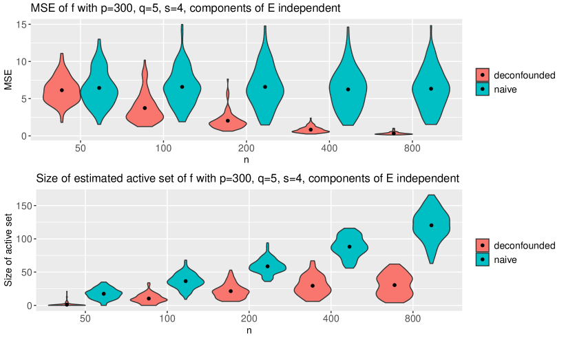
Figure 2: MSE (top) and size of estimated active set (bottom) for $\Sigma_{E}=I_{p}$ and varying $n$.

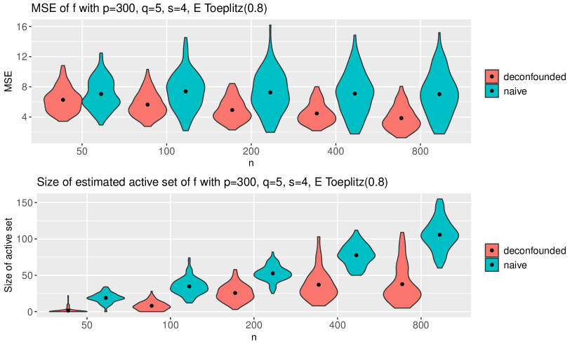
Figure 3: MSE (top) and size of estimated active set (bottom) for $\Sigma_{E}=\textup{Toeplitz}(0.8)$ and varying $n$.

4.2.2 Varying $p$

Here, we fix $n=300$ and $q=5$ and vary $p$ between $p=50$ and $p=800$. For each $p$, we simulate $100$ data sets. In Figure 4, we see the resulting MSE of $\hat{f}$ on top and the size of the estimated active set on the bottom for a covariance matrix $\Sigma_{E}=I_{p}$. In Figure 5, we see the same plot for $\Sigma_{E}=\textup{Toeplitz}(0.8)$. The picture is similar to before: The deconfounded method is clearly superior to the naive method both in terms of MSE and in terms of the size of the estimated active set for all values of $p$.

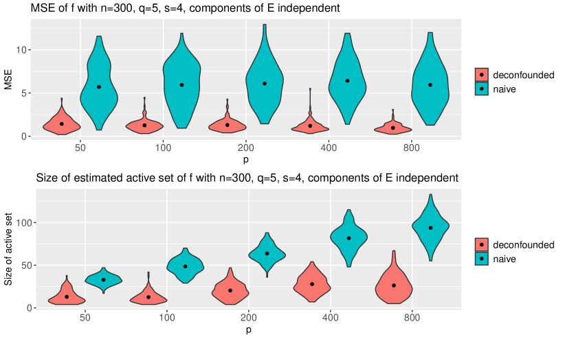
Figure 4: MSE (top) and size of estimated active set (bottom) for $\Sigma_{E}=I_{p}$ and varying $p$.

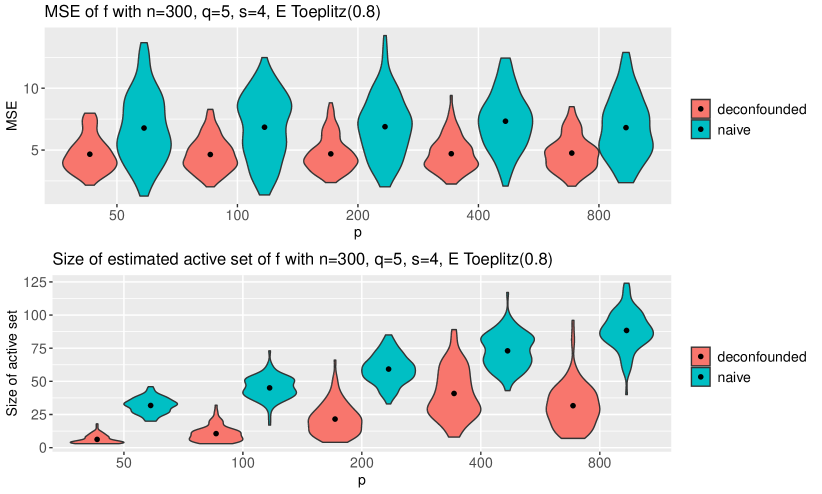
Figure 5: MSE (top) and size of estimated active set (bottom) for $\Sigma_{E}=\textup{Toeplitz}(0.8)$ and varying $p$.

4.2.3 Varying the Strength of Confounding

Here, we fix $n=400$, $p=500$, $q=5$ and $\Sigma_{E}=I_{p}$. We also use the previous setting but vary the strength of confounding, i.e. the entries of $\psi\in\mathbb{R}^{q}$ are sampled i.i.d. $\textup{Unif}[0,cs]$ with the confounding strength $cs$ between $0$ and $3$. For each value of $cs$, we simulate $50$ data sets. In Figure 6, we see the resulting MSE of $\hat{f}$ on top and the size of the estimated active set on the bottom. We observe that for very small confounding strength ($cs\leq 0.5$), the deconfounded method performs slightly worse than the naive method. This is to be expected since by using the trim transformation we loose a bit of signal. However, as the confounding increases, the deconfounded method is much more robust than the naive method.

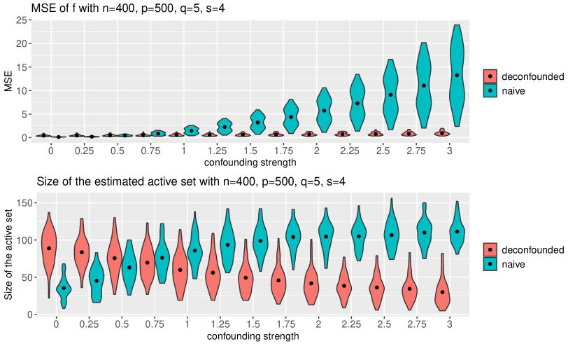
Figure 6: MSE (top) and size of estimated active set (bottom) for varying confounding strength.

4.2.4 Varying the Proportion of Confounded Covariates

We investigate the effect of the denseness assumption by varying the proportion of confounded covariates. For this, we fix $n=400$, $p=500$, $q=5$ and $\Sigma_{E}=I_{p}$. We keep the setting described in Section 4.2 but the entries of the matrix $\Psi$ are now i.i.d. $\textup{Unif}[-1,1]\cdot\textup{Bernoulli}(prop)$, where $prop\in[0,1]$ is the proportion of confounded covariates. That is, a fraction of $1-prop$ of the entries of $\Psi$ are set to $0$. For each value of $prop$, we simulate 50 data sets. The same plots as before can be found in Figure 7. The setting of $prop=0$ corresponds to $X=E$, that is, the confounding does not affect $X$. Hence, the contribution $\psi^{T}H$ is an error term independent of $X$. We observe that in this setting, the deconfounded method performs slightly worse than the naive method, as there is still some signal removed by using a spectral transformation. On the other hand, we see from the plot that the deconfounded method outperforms the naive method even if the confounding only affects a very small proportion of the covariates. We conclude that deconfounding is useful also if the confounding is not very dense.

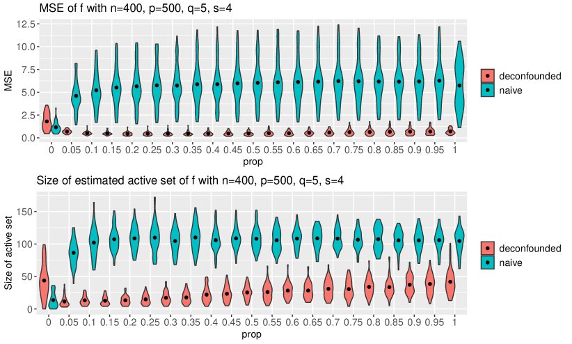
Figure 7: MSE (top) and size of the estimated active set (bottom) for varying proportion of confounded covariates.

4.2.5 Nonlinear Confounding Effects

We now consider the following mis-specified version of (2), where the confounding acts potentially nonlinearly on both $X$ and $Y$.

$$Y=f^{0}(X)+\eta_{\beta}(H^{T}\psi)+e\text{ and }X_{j}=\eta_{\alpha}(\Psi_{j}^{T}H)+E_{j},\,j=1,\ldots,p,$$

for some nonlinear functions $\eta_{\alpha},\eta_{\beta}:\mathbb{R}\to\mathbb{R}$. For our simulations, we use the family of functions $\eta_{\alpha}(t)=(1-\alpha)t+\alpha|t|,\,\alpha\in[0,1]$, that is $\eta_{\alpha}(t)$ interpolates between $t$ and $|t|$. Otherwise, we use the setup from Section 4.2. As before, we fix $n=400$, $p=500$, $q=5$ and $\Sigma_{E}=I_{p}$. We vary $\alpha$ and $\beta$ on a grid of values in $[0,1]$ and simulate $50$ data sets for each setting and calculate the mean squared errors $\|\hat{f}-f^{0}\|_{L_{2}}^{2}$ for the deconfounded method and the naive method. In Figure 8, we report the ratio of the average MSE for the deconfounded method and the average MSE of the naive method, where the averages are taken over the $50$ simulated data sets. Values less than $1$ indicate a smaller average MSE for the deconfounded method, whereas values larger than $1$ indicate that the naive method has a smaller average MSE. We see that for a wide range of combinations of $\alpha$ and $\beta$, the results are in favor of the deconfounded method. We observe that deconfounding slightly worsens the performance of the algorithm only if $\alpha$ is close to $1$ and $\beta$ close to $0$ (i.e. the confounding acts very nonlinearly on $X$ and almost linearly on $Y$ or if $\alpha$ is close to $0$ and $\beta$ is close to $1$ (i.e. the confounding acts almost linearly on $X$ and very nonlinearly on $Y$). Intuitively, in such settings, the contribution of the confounding to $X$ is almost orthogonal to the contribution of the confounding to $Y$; hence, applying the trim transformation is not helpful in such settings. However, we see that for slightly to moderately nonlinear confounding effects in $X$ and $Y$, applying the deconfounded method always improves the performance compared to the naive method.

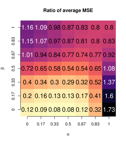
Figure 8: Ratio of average MSE for the deconfounded method and average MSE for the naive method. Values smaller than $1$ are in favor of the deconfounded method, whereas values larger than $1$ are in favor of the naive method.

4.2.6 Summarizing the Simulation Results

The simulations indicate that applying spectral deconfounding significantly improves the robustness of high-dimensional additive models. If there is no confounding, the deconfounded method performs slightly worse than the naive method. If there is dense confounding, one gains a lot, both in terms of prediction of $f^{0}$ and in terms of variable screening. If there is only moderately dense confounding, or if the model is moderately mis-specified in another way, it is still better to apply deconfounding than to do nothing.

4.3 Real Data Analysis

We apply our method to the motif regression problem. We use a data set that has previously been analyzed by [18], whose results indicate that a (nonlinear) additive model might be appropriate. The data set originally comes from [2] and has also been reexamined by [36]. We use the same $\mathbf{X}$ and $\mathbf{Y}$ as in [18], that is, the rows of $\mathbf{X}\in\mathbb{R}^{2587\times 666}$ are the scores of 666 motifs and the entries of $\mathbf{Y}\in\mathbb{R}^{2587}$ are the gene expression values of the corresponding $n=2587$ genes under a particular condition. In Figure 9, we plot the singular values of $\mathbf{X}$, where we center the columns of $\mathbf{X}$ to have mean zero. We see that we have one very large spike and several smaller spikes in the singular values. This indicates that confounding might be present. We apply the deconfounded method ($Q=Q^{\text{trim}})$ and the naive method ($Q=I_{n}$) on the data set. The fitted function for $Q=Q^{\text{trim}}$ has 95 active variables, whereas the fitted function for $Q=I_{n}$ has 211 active variables. The intersection of the two estimated active sets has cardinality 92. In Figure 10, we plot the fitted functions $\hat{f}_{j}$ for the variables $X_{j}$ whose effects are the strongest (measured by the norm of the coefficient vector $\|\hat{\beta}_{j}\|_{2}$ of $\hat{f}_{j}(\cdot)=b_{j}(\cdot)^{T}\hat{\beta}_{j}$), when estimated using the deconfounded method. In Figure 11, we plot the fitted functions $\hat{f}_{j}$ for the indices $j$ such that the effects of $\hat{f}_{j}$ estimated using the naive method are the strongest among the $j$ which are not in the active set estimated using the deconfounded method. Finally, Figure 12 displays the order of importance of the covariates: it shows very clearly that very quickly, the top selected covariates do not exhibit strong correspondence to each other and hence, the difference between the methods cannot be explained by a simple thresholding rule. In view of this, we believe that the variable importance and selection with the deconfounded method leads to much better results for this data set with spiked singular values as shown in Figure 9.

Figure 9: Singular values of centered motif scores.

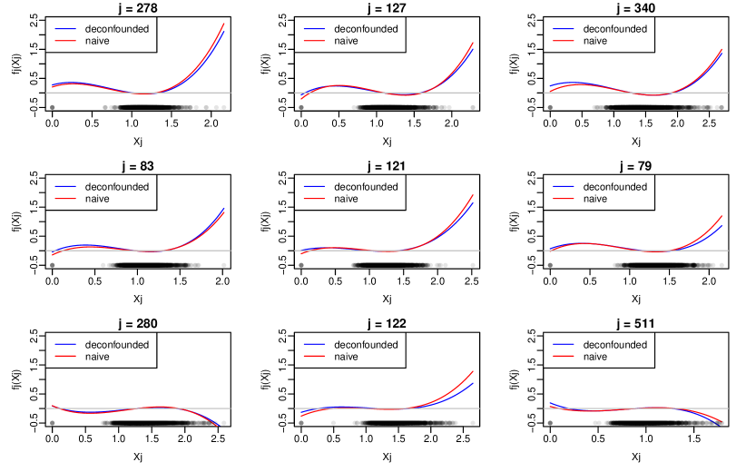
Figure 10: Motif data set. Fitted functions $\hat{f}_{j}$ for the covariates $X_{j}$ with strongest effect estimated using the deconfounded method. The grey dots indicate the observed values of $X_{j}$.

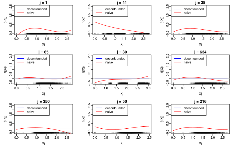
Figure 11: Motif data set. Fitted functions $\hat{f}_{j}$ for the covariates $X_{j}$ with zero estimated effect by the deconfounded method but strongest estimated effect by the naive method. The grey dots indicate the observed values of $X_{j}$.

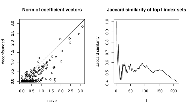
Figure 12: Comparison of the strength of the fitted functions (measured by the norm of the coefficient vector $\|\hat{\beta}_{j}\|_{2}$ of $\hat{f}_{j}(\cdot)=b_{j}(\cdot)^{T}\hat{\beta}_{j}$) for the motif data set. Left: Strength of the fitted functions estimated using the deconfounded method vs. strength of the fitted functions estimated using the naive method. Right: Jaccard similarity $\frac{|\mathcal{T}_{dec}^{(l)}\cap\mathcal{T}_{naive}^{(l)}|}{|\mathcal{T}_{dec}^{(l)}\cup\mathcal{T}_{naive}^{(l)}|}$ vs. $l$ with $\mathcal{T}_{dec}^{(l)}\subset\{1,\ldots,p\}$ being the indices of the $l$ strongest fitted functions using the deconfounded method and $\mathcal{T}_{naive}^{(l)}$ the indices of the $l$ strongest fitted functions using the naive method.

5 Discussion

We developed novel theory and methodology for fitting high-dimensional additive models in presence of hidden confounding. With this, we established that spectral transformations introduced by [8] can also be used in the context of nonlinear regression. Our rigorous theoretical development covers convergence rates as well as detailed justification of high-level assumptions such as the compatibility condition. We demonstrated good empirical performance of our procedure on a wide range of simulation scenarios as well as on real data. In case of no hidden confounding, the method is slightly worse than plain sparse additive model fitting. In presence of hidden confounding though, there is much to be gained, even if the model is moderately mis-specified or the assumptions are not fully satisfied.

Our work indicates that the extension of using spectral transformations with arbitrary machine learning algorithms could be possible. A general path for such extensions is to replace least squares type objectives $\arg\min_{f\in\mathcal{F}}\|\mathbf{Y}-\mathbf{f}(\mathbf{X})\|_{2}^{2}/n$, where $\mathcal{F}$ is some function class, by their deconfounded version $\arg\min_{f\in\mathcal{F}}\|Q(\mathbf{Y}-\mathbf{f}(\mathbf{X}))\|_{2}^{2}/n$ as we did it for the function class of additive models. A rigorous and detailed theoretical understanding will be challenging, but some of our developed results may be useful for such an analysis.

Appendix A Proofs of Theorem 1 and Corollary 3

A.1 Proof of Theorem 1

We first show that the functions $\hat{f}_{j}$ are empirically centered. This is an implication of Assumption 3 (partition of unity). For all $\gamma_{1},\ldots,\gamma_{p}\in\mathbb{R}$, we have the equality

$$\frac{1}{n}\left\|Q(\mathbf{Y}-\hat{\beta}_{0}\mathbf{1}_{n}-\sum_{j=1}^{p}B^{(j)}\hat{\beta}_{j})\right\|_{2}^{2}=\frac{1}{n}\left\|Q(\mathbf{Y}-(\hat{\beta}_{0}+\sum_{j=1}^{p}\gamma_{j})\mathbf{1}_{n}-\sum_{j=1}^{p}B^{(j)}(\hat{\beta}_{j}-\gamma_{j}\mathbf{1}_{K}))\right\|_{2}^{2}$$

for the first term in the objective (4). Since $\hat{\beta}$ is the minimizer of (4), we must have that it minimizes the penalty term. Hence, for $j=1,\ldots,p$, we have $\frac{\textup{d}}{\textup{d}\gamma_{j}}\rvert_{\gamma_{j}=0}\|B^{(j)}(\hat{\beta}_{j}+\gamma_{j}\mathbf{1}_{K})\|_{2}^{2}=0$. This implies that $\mathbf{1}_{K}^{T}(B^{(j)})^{T}B^{(j)}\hat{\beta}_{j}=0$. Using again the partition of unity, we have that $B^{(j)}\hat{\beta}_{j}=0$. Hence, the estimated functions $\hat{f}_{j}$ are empirically centered, i.e. $\sum_{i=1}^{n}\hat{f}_{j}(x_{i,j})=0$.

For $j=1,\ldots p$, consider functions $f_{j}^{c}(\cdot)=b_{j}(\cdot)^{T}\beta_{j}^{c}$ that are empirically centered, i.e. $\sum_{i=1}^{n}f_{j}^{c}(x_{i,j})=0$. Also define $\beta_{0}^{c}=\beta_{0}^{0}$. For $j\notin\mathcal{T}$, let $f_{j}^{c}=0$. In the end, we will set $f_{j}^{c}(\cdot)=f_{j}^{\ast}(\cdot)-\frac{1}{n}\sum_{i=1}^{n}f_{j}^{\ast}(x_{i,j})$ and $\beta_{j}^{c}=\beta_{j}^{\ast}-(\frac{1}{n}\sum_{i=1}^{n}f_{j}^{\ast}(x_{i,j}))\mathbf{1}_{K}$.

We now follow the strategy of the proof of Proposition 5 in [19]. By the definition of $\hat{\beta}$, we have

$$\frac{1}{n}\left\|Q(\mathbf{Y}-\hat{\beta}_{0}\mathbf{1}_{n}-\sum_{j=1}^{p}B^{(j)}\hat{\beta}_{j})\right\|_{2}^{2}+\frac{\lambda}{\sqrt{n}}\sum_{j=1}^{p}\|B^{(j)}\hat{\beta}_{j}\|_{2}$$

$$\leq\frac{1}{n}\left\|Q(\mathbf{Y}-\beta_{0}^{c}\mathbf{1}_{n}-\sum_{j=1}^{p}B^{(j)}\beta_{j}^{c})\right\|_{2}^{2}+\frac{\lambda}{\sqrt{n}}\sum_{j=1}^{p}\|B^{(j)}\beta_{j}^{c}\|_{2}$$

We use decomposition (6) to write

$$\mathbf{Y}-\hat{\beta}_{0}\mathbf{1}_{n}-\sum_{j=1}^{p}B^{(j)}\hat{\beta}_{j}=\mathbf{X}b+\bm{\epsilon}+(\beta_{0}^{c}-\hat{\beta}_{0})\mathbf{1}_{n}+\sum_{j=1}^{p}B^{(j)}(\beta_{j}^{c}-\hat{\beta}_{j})+\sum_{j=1}^{p}(\mathbf{f}_{j}^{0}-\mathbf{f}_{j}^{c}).$$

It follows that

$$\frac{1}{n}\|Q((\beta_{0}^{c}-\hat{\beta}_{0})\mathbf{1}_{n}+\sum_{j=1}^{p}B^{(j)}(\beta_{j}^{c}-\hat{\beta}_{j}))\|_{2}^{2}+\frac{\lambda}{\sqrt{n}}\sum_{j=1}^{p}\|B^{(j)}\hat{\beta}_{j}\|_{2}$$

$$\leq\frac{\lambda}{\sqrt{n}}\sum_{j=1}^{p}\|B^{(j)}\beta_{j}^{c}\|_{2}-\frac{2}{n}\left(\mathbf{X}b+\bm{\epsilon}+\sum_{j=1}^{p}(\mathbf{f}_{j}^{0}-\mathbf{f}_{j}^{c})\right)^{T}Q^{2}\left((\beta_{0}^{c}-\hat{\beta}_{0})\mathbf{1}_{n}+\sum_{j=1}^{p}B^{(j)}(\beta_{j}^{c}-\hat{\beta}_{j})\right)$$ (17)

We use a reparametrization: Let $R_{j}\in\mathbb{R}^{K\times K}$ such that $R_{j}^{T}R_{j}=\frac{1}{n}(B^{(j)})^{T}B^{(j)}$ and define $\tilde{\beta}_{j}=R_{j}\beta_{j}$ and $\tilde{B}^{(j)}=B^{(j)}R_{j}^{-1}$. Then $\tilde{B}^{(j)}\tilde{\beta}_{j}=B^{(j)}\beta_{j}$ and $(\tilde{B}^{(j)})^{T}\tilde{B}^{(j)}=nI_{K}$. Moreover,

$$\frac{1}{\sqrt{n}}\sum_{j=1}^{p}\left\|B^{(j)}\beta_{j}\right\|_{2}=\sum_{j=1}^{p}\|\tilde{\beta}_{j}\|_{2}.$$

Note that using the Cauchy-Schwarz inequality

$$\left|\frac{2}{n}\bm{\epsilon}^{T}Q^{2}\sum_{j=1}^{p}B^{(j)}(\beta_{j}^{c}-\hat{\beta}_{j})\right| =\left|\frac{2}{n}\bm{\epsilon}^{T}Q^{2}\sum_{j=1}^{p}\tilde{B}^{(j)}(\tilde{\beta}_{j}^{c}-\tilde{\hat{\beta}}_{j})\right|$$

$$\leq\frac{2}{n}\sum_{j=1}^{p}\|(\tilde{B}^{(j)})^{T}Q^{2}\bm{\epsilon}\|_{2}\|\tilde{\beta}_{j}^{c}-\tilde{\hat{\beta}}_{j}\|_{2}$$

$$\leq\frac{2}{n}\max_{j=1,\ldots,p}\|(\tilde{B}^{(j)})^{T}Q^{2}\bm{\epsilon}\|_{2}\sum_{j=1}^{p}\|\tilde{\beta}_{j}^{c}-\tilde{\hat{\beta}}_{j}\|_{2}$$ (18)

and also

$$\left|\frac{2}{n}\bm{\epsilon}^{T}Q^{2}(\beta_{0}^{c}-\hat{\beta}_{0})\mathbf{1}_{n}\right|=\frac{2}{n}|\bm{\epsilon}^{T}Q^{2}\mathbf{1}_{n}||\beta_{0}^{c}-\hat{\beta}_{0}|$$ (19)

For some constant $c>0$, let $\lambda_{0}=\lambda/(1+c)$ and $A_{0}=A/(1+c)$ and define the event

$$\mathcal{A}=\left\{\max\left(\frac{2}{n}|\bm{\epsilon}^{T}Q^{2}\mathbf{1}_{n}|,\frac{2}{n}\max_{j=1,\ldots,p}\|(\tilde{B}^{(j)})^{T}Q^{2}\bm{\epsilon}\|_{2}\right)\leq\lambda_{0}\right\}.$$

The goal is to show that $\mathcal{A}$ has high probability for $n\to\infty$. Recall from decomposition (6) that $\bm{\epsilon}=\bm{e}+\Delta$ with $\Delta_{i}=h_{i}^{T}\psi-x_{i}^{T}b$. By Hoeffding’s inequality (see for example Theorem 2.6.3 in 33) applied conditionally on $\mathbf{X}$, there exists $c^{\prime}>0$ such that

$$\mathbb{P}\left(\frac{2}{n}|\bm{e}^{T}Q^{2}\mathbf{1}_{n}|>A_{0}C_{0}\sqrt{\frac{K\log p}{n}}|\mathbf{X}\right) \leq 2\exp\left(\frac{-c^{\prime}A_{0}^{2}C_{0}^{2}Kn\log p}{4\|e\|_{\psi_{2}}^{2}\|Q^{2}\mathbf{1}_{n}\|_{2}^{2}}\right)$$

$$\leq 2\exp\left(\frac{-c^{\prime}A_{0}^{2}K\log p}{4}\right)$$

$$\leq 2p^{-c^{\prime}A_{0}^{2}K/4}.$$ (20)

Since the bound is not depending on $\mathbf{X}$, it also holds for the unconditional probability. Define $t_{n}=\frac{1}{2}A_{0}C_{0}\sqrt{nK\log p}$. For $t_{n}^{2}\geq\|(\tilde{B}^{(j)})^{T}Q^{2}\|_{F}^{2}(C_{0}^{2}+\sigma_{e}^{2})$, we have by the union bound and Lemma 14 below (applied conditionally on $\mathbf{X}$), that there exists $c^{\prime\prime}>0$ such that

$$\mathbb{P}\left(\frac{2}{n}\max_{j=1,\ldots,p}\|(\tilde{B}^{(j)})^{T}Q^{2}\mathbf{e}\|_{2}>A_{0}C_{0}\sqrt{\frac{K\log p}{n}}|\mathbf{X}\right) \leq\sum_{j=1}^{p}\mathbb{P}\left(\|(\tilde{B}^{(j)})^{T}Q^{2}\mathbf{e}\|_{2}>t_{n}|\mathbf{X}\right)$$

$$\leq\sum_{j=1}^{p}2\exp\left[-c^{\prime\prime}\left(\frac{t_{n}^{2}}{C_{0}^{2}\|(\tilde{B}^{(j)})^{T}Q^{2}\|_{F}^{2}}-\frac{\sigma_{e}^{2}}{C_{0}^{2}}\right)\right]$$

Since the singular values of $Q$ are bounded by $1$, we have by von Neumann’s trace inequality [26],

$$\|(\tilde{B}^{(j)})^{T}Q^{2}\|_{F}^{2}=\operatorname{tr}((\tilde{B}^{(j)})^{T}Q^{4}\tilde{B}^{(j)})=\operatorname{tr}(Q^{4}\tilde{B}^{(j)}(\tilde{B}^{(j)})^{T})\leq\operatorname{tr}(\tilde{B}^{(j)}(\tilde{B}^{(j)})^{T})=\operatorname{tr}((\tilde{B}^{(j)})^{T}\tilde{B}^{(j)})=nK.$$

Hence for $t_{n}^{2}\geq nK(C_{0}^{2}+\sigma_{e}^{2})$ and plugging in the definition of $t_{n}$,

$$\mathbb{P}\left(\frac{2}{n}\max_{j=1,\ldots,p}\|(\tilde{B}^{(j)})^{T}Q^{2}\mathbf{e}\|_{2}>A_{0}C_{0}\sqrt{\frac{K\log p}{n}}\right) \leq 2p\exp\left[-c^{\prime\prime}\left(\frac{t_{n}^{2}}{nKC_{0}^{2}}-\frac{\sigma_{e}^{2}}{C_{0}^{2}}\right)\right]$$

$$=2p\exp\left(c^{\prime\prime}\frac{\sigma_{e}^{2}}{C_{0}^{2}}\right)\exp\left(\frac{c^{\prime\prime}}{4}A_{0}^{2}\log p\right)$$

$$=2\exp\left(c^{\prime\prime}\frac{\sigma_{e}^{2}}{C_{0}^{2}}\right)p^{1-c^{\prime\prime}A_{0}^{2}/4}$$ (21)

Hence, we can choose $A_{0}^{2}>\max\left(\frac{4}{c^{\prime\prime}},4\frac{C_{0}^{2}+\sigma_{e}^{2}}{C_{0}^{2}\log p}\right)$.

On the other hand, since $(\tilde{B}^{(j)})^{T}\tilde{B}^{(j)}=nI_{K}$ and $\|Q\|_{op}\leq 1$,

$$\|(\tilde{B}^{(j)})^{T}Q^{2}\Delta\|_{2}\leq\|(\tilde{B}^{(j)})^{T}Q^{2}\|_{op}\|\Delta\|_{2}\leq\|\tilde{B}^{(j)}\|_{op}\|\Delta\|_{2}\leq\sqrt{n}\|\Delta\|_{2}.$$

Together with Markov’s inequality, we obtain for $t>0$

$$\mathbb{P}\left(\frac{2}{n}\max_{j=1,\ldots,p}\|(\tilde{B}^{(j)})^{T}Q^{2}\Delta\|_{2}>t\right) \leq\mathbb{P}\left(\frac{2}{\sqrt{n}}\|\Delta\|_{2}>t\right)$$

$$\leq\frac{4\mathbb{E}[\|\Delta\|_{2}^{2}]}{nt^{2}}.$$

From the definition (5) of $b$ and using Assumption 1, we get that

$$\frac{1}{n}\mathbb{E}[\|\Delta\|_{2}^{2}] =\mathbb{E}[\Delta_{i}^{2}]$$

$$=\mathbb{E}[(\psi^{T}H-b^{T}X)^{2}]$$

$$=\mathbb{E}[(\psi^{T}(H-\Psi\mathbb{E}[XX^{T}]^{-1}X))^{2}]$$

$$=\psi^{T}(I_{q}-\Psi\mathbb{E}[XX^{T}]^{-1}\Psi^{T})\psi$$

By Lemma 15 below, we arrive at

$$\frac{1}{n}\mathbb{E}[\|\Delta\|_{2}^{2}]\lesssim\frac{\|\psi\|_{2}^{2}}{1+\lambda_{q}^{2}(\Psi)}.$$

Hence by condition (10) on $\lambda_{2}$,

$$\mathbb{P}\left(\frac{2}{n}\max_{j=1,\ldots,p}\|(\tilde{B}^{(j)})^{T}Q^{2}\Delta\|_{2}>\frac{1}{1+c}\lambda_{2}\right)\lesssim\frac{\|\psi\|_{2}^{2}}{1+\lambda_{q}^{2}(\Psi)}/\lambda_{2}^{2}=o(1).$$

Similarly, also

$$\mathbb{P}\left(\frac{2}{n}|\Delta^{T}Q^{2}\mathbf{1}_{n}|>\frac{1}{1+c}\lambda_{2}\right)\lesssim\frac{\|\psi\|_{2}^{2}}{1+\lambda_{q}^{2}(\Psi)}/\lambda_{2}^{2}=o(1).$$

From this, (20) and (21), we get that $\mathbb{P}(\mathcal{A})>1-o(1)$. In the following, we establish (11) on the event $\mathcal{A}$. Together with (18) and (19), we get from (17) that on the event $\mathcal{A}$, we have

$$\frac{1}{n}\|Q((\beta_{0}^{c}-\hat{\beta}_{0})\mathbf{1}_{n}+\sum_{j=1}^{p}B^{(j)}(\beta_{j}^{c}-\hat{\beta}_{j}))\|_{2}^{2}+\lambda\sum_{j=1}^{p}\|\tilde{\hat{\beta}}_{j}\|_{2}$$

$$\leq\lambda\sum_{j=1}^{p}\|\tilde{\beta}_{j}^{c}\|_{2}+\lambda_{0}\left(|\beta_{0}^{c}-\hat{\beta}_{0}|+\sum_{j=1}^{p}\|\tilde{\beta}_{j}^{c}-\tilde{\hat{\beta}}_{j}\|_{2}\right)+U_{n}$$

With

$$U_{n}=\left|\frac{2}{n}\left(\mathbf{X}b+\sum_{j=1}^{p}(\mathbf{f}_{j}^{0}-\mathbf{f}_{j}^{c})\right)^{T}Q^{2}\left((\beta_{0}^{c}-\hat{\beta}_{0})\mathbf{1}_{n}+\sum_{j=1}^{p}B^{(j)}(\beta_{j}^{c}-\hat{\beta}_{j})\right)\right|.$$

Recall that $\beta_{j}^{c}=0$ for all $j\in\mathcal{T}^{c}$. By the triangle inequality,

$$\sum_{j\in\mathcal{T}}\|\tilde{\beta}_{j}^{c}\|_{2}-\sum_{j\in\mathcal{T}}\|\tilde{\hat{\beta}}_{j}\|_{2}\leq\sum_{j\in\mathcal{T}}\|\tilde{\beta}_{j}^{c}-\tilde{\hat{\beta}}_{j}\|_{2},\text{ and }\sum_{j\in\mathcal{T}^{c}}\|\tilde{\hat{\beta}}_{j}\|_{2}=\sum_{j\in\mathcal{T}^{c}}\|\tilde{\beta}_{j}^{c}-\tilde{\hat{\beta}}_{j}\|_{2}.$$

It follows that

$$\frac{1}{n}\|Q((\beta_{0}^{c}-\hat{\beta}_{0})\mathbf{1}_{n}+\sum_{j=1}^{p}B^{(j)}(\beta_{j}^{c}-\hat{\beta}_{j}))\|_{2}^{2}+(\lambda-\lambda_{0})\sum_{j\in\mathcal{T}^{c}}\|\tilde{\hat{\beta}}_{j}\|_{2}$$

$$\leq\lambda\left(\sum_{j\in\mathcal{T}}\|\tilde{\beta}_{j}^{c}\|-\sum_{j\in\mathcal{T}}\|\tilde{\hat{\beta}}_{j}\|_{2}\right)+\lambda_{0}\left(|\beta_{0}^{c}-\hat{\beta}_{0}|+\sum_{j\in\mathcal{T}}\|\tilde{\beta}_{j}^{c}-\tilde{\hat{\beta}}_{j}\|_{2}\right)+U_{n}$$

$$\leq(\lambda+\lambda_{0})\left(|\beta_{0}^{c}-\hat{\beta}_{0}|+\sum_{j\in\mathcal{T}}\|\tilde{\beta}_{j}^{c}-\tilde{\hat{\beta}}_{j}\|_{2}\right)+U_{n}.$$

We consider two cases:

Case 1:

$$(\lambda+\lambda_{0})\left(|\beta_{0}^{c}-\hat{\beta}_{0}|+\sum_{j\in\mathcal{T}}\|\tilde{\beta}_{j}^{c}-\tilde{\hat{\beta}}_{j}\|_{2}\right)\geq U_{n},$$

Case 2:

$$(\lambda+\lambda_{0})\left(|\beta_{0}^{c}-\hat{\beta}_{0}|+\sum_{j\in\mathcal{T}}\|\tilde{\beta}_{j}^{c}-\tilde{\hat{\beta}}_{j}\|_{2}\right)<U_{n}.$$ (22)

In Case 1, we have

$$\frac{1}{n}\|Q((\beta_{0}^{c}-\hat{\beta}_{0})\mathbf{1}_{n}+\sum_{j=1}^{p}B^{(j)}(\beta_{j}^{c}-\hat{\beta}_{j}))\|_{2}^{2}+(\lambda-\lambda_{0})\sum_{j\in\mathcal{T}^{c}}\|\tilde{\hat{\beta}}_{j}\|_{2}\leq 2(\lambda+\lambda_{0})\left(|\beta_{0}^{c}-\hat{\beta}_{0}|+\sum_{j\in\mathcal{T}}\|\tilde{\beta}_{j}^{c}-\tilde{\hat{\beta}}_{j}\|_{2}\right)$$ (23)

and in particular

$$\sum_{j\in\mathcal{T}^{c}}\|\tilde{\hat{\beta}}_{j}\|_{2}\leq\frac{4+2c}{c}\left(|\beta_{0}^{c}-\hat{\beta}_{0}|+\sum_{j\in\mathcal{T}}\|\tilde{\beta}_{j}^{c}-\tilde{\hat{\beta}}_{j}\|_{2}\right).$$ (24)

By the definition of $\tilde{\hat{\beta}}_{j}$, it follows that $\|\tilde{\hat{\beta}}_{j}\|_{2}=\frac{1}{\sqrt{n}}\|B^{(j)}\beta_{j}\|_{2}=\frac{1}{\sqrt{n}}\|\hat{\mathbf{f}}_{j}\|_{2}$ and similarly $\|\tilde{\beta}_{j}^{c}-\tilde{\hat{\beta}}_{j}\|_{2}=\frac{1}{\sqrt{n}}\|\mathbf{f}_{j}^{c}-\hat{\mathbf{f}}_{j}\|_{2}$. Hence, we can rewrite (24) as

$$\sum_{j\in\mathcal{T}^{c}}\frac{1}{\sqrt{n}}\|\mathbf{f}_{j}^{c}-\hat{\mathbf{f}}_{j}\|_{2}\leq\frac{4+2c}{c}\left(|\beta_{0}^{c}-\hat{\beta}_{0}|+\sum_{j\in\mathcal{T}}\frac{1}{\sqrt{n}}\|\mathbf{f}_{j}^{c}-\hat{\mathbf{f}}_{j}\|_{2}\right).$$ (25)

This means that for $M=(4+2c)/c$, the function $f^{c}-\hat{f}=(\beta_{0}^{c}-\hat{\beta}_{0})+\sum_{j=1}^{p}(f_{j}^{c}-\hat{f}_{j})$ lies in the set $\mathcal{F}_{M,\mathcal{T}}^{n}$ defined in (8) (recall from the beginning of the proof that $\hat{f}_{j}$ and $f_{j}^{c}$ are empirically centered for all $j=1,\ldots,p$). By the definition (9) of the compatibility constant $\tau_{n}$, we have that

$$\frac{1}{n}\|Q((\beta_{j}^{c}-\hat{\beta}_{j})\mathbf{1}_{n}+\sum_{j=1}^{p}B^{(j)}(\beta_{j}^{c}-\hat{\beta}_{j}))\|_{2}^{2}=\frac{1}{n}\|Q(\mathbf{f}^{c}-\hat{\mathbf{f}})\|_{2}^{2}\geq\tau_{n}\left((\beta_{0}^{c}-\hat{\beta}_{0})^{2}+\sum_{j=1}^{p}\frac{1}{n}\|\mathbf{f}_{j}^{c}-\hat{\mathbf{f}}_{j}\|_{2}^{2}\right).$$

Together with the Cauchy-Schwarz inequality and (23), we have

$$\tau_{n}\left(|\beta_{0}^{c}-\hat{\beta}_{0}|+\sum_{j\in\mathcal{T}}\frac{1}{\sqrt{n}}\|\mathbf{f}_{j}^{c}-\hat{\mathbf{f}}_{j}\|_{2}\right)^{2} \leq(s+1)\tau_{n}\left((\beta_{0}^{c}-\hat{\beta}_{0})^{2}+\sum_{j=1}^{p}\frac{1}{n}\|\mathbf{f}_{j}^{\ast}-\hat{\mathbf{f}}_{j}\|_{2}^{2}\right)$$

$$\leq(s+1)\frac{1}{n}\|Q((\beta_{j}^{c}-\hat{\beta}_{j})\mathbf{1}_{n}+\sum_{j=1}^{p}B^{(j)}(\beta_{j}^{c}-\hat{\beta}_{j}))\|_{2}^{2}$$

$$\leq 2(s+1)(\lambda+\lambda_{0})\left(|\beta_{0}^{c}-\hat{\beta}_{0}|+\sum_{j\in\mathcal{T}}\|\tilde{\beta}_{j}^{c}-\tilde{\hat{\beta}}_{j}\|_{2}\right)$$

$$=2(s+1)(\lambda+\lambda_{0})\left(|\beta_{0}^{c}-\hat{\beta}_{0}|+\sum_{j\in\mathcal{T}}\frac{1}{\sqrt{n}}\|\mathbf{f}_{j}^{c}-\hat{\mathbf{f}}_{j}\|_{2}\right)$$

and hence,

$$|\beta_{0}^{c}-\hat{\beta}_{0}|+\sum_{j\in\mathcal{T}}\frac{1}{\sqrt{n}}\|\mathbf{f}_{j}^{\ast}-\hat{\mathbf{f}}_{j}\|_{2}\leq\frac{2(s+1)(\lambda+\lambda_{0})}{\tau_{n}}.$$

Together with (25), we arrive at

$$|\beta_{0}^{c}-\hat{\beta}_{0}|+\sum_{j=1}^{p}\frac{1}{\sqrt{n}}\|\mathbf{f}_{j}^{\ast}-\hat{\mathbf{f}}_{j}\|_{2}\lesssim\frac{s\lambda}{\tau_{n}}.$$ (26)

In Case 2, we have

$$\frac{1}{n}\|Q((\beta_{0}^{c}-\hat{\beta}_{0})\mathbf{1}_{n}+\sum_{j=1}^{p}B^{(j)}(\beta_{j}^{c}-\hat{\beta}_{j}))\|_{2}^{2}+(\lambda-\lambda_{0})\sum_{j\in\mathcal{T}^{c}}\|\tilde{\hat{\beta}}_{j}\|_{2}\leq 2U_{n}.$$ (27)

By the Cauchy-Schwarz inequality,

$$2U_{n}\leq\frac{4}{n}\|Q\mathbf{X}b+Q\sum_{j=1}^{p}(\mathbf{f}_{j}^{0}-\mathbf{f}_{j}^{c})\|_{2}\|Q((\beta_{0}^{c}-\hat{\beta}_{0})\mathbf{1}_{n}+\sum_{j=1}^{p}B^{(j)}(\beta_{j}^{c}-\hat{\beta}_{j}))\|_{2}$$ (28)

In particular, it follows from (27) and (28) that

$$\frac{1}{\sqrt{n}}\|Q((\beta_{0}^{c}-\hat{\beta}_{0})\mathbf{1}_{n}+\sum_{j=1}^{p}B^{(j)}(\beta_{j}^{c}-\hat{\beta}_{j}))\|_{2}\leq\frac{4}{\sqrt{n}}\|Q\mathbf{X}b+Q\sum_{j=1}^{p}(\mathbf{f}_{j}^{0}-\mathbf{f}_{j}^{c})\|_{2}.$$

Plugging this back into (28), yields

$$2U_{n}\leq\frac{16}{n}\|Q\mathbf{X}b+Q\sum_{j=1}^{p}(\mathbf{f}_{j}^{0}-\mathbf{f}_{j}^{c})\|_{2}^{2}.$$

From (22) and (27), we have

$$\sum_{j=1}^{p}\|\tilde{\beta}_{j}^{c}-\tilde{\hat{\beta}}_{j}\|_{2}\leq\frac{U_{n}}{(\lambda+\lambda_{0})}+\frac{2U_{n}}{(\lambda-\lambda_{0})}.$$

Hence, using again that $\|\tilde{\beta}_{j}^{c}-\tilde{\hat{\beta}}_{j}\|_{2}=\frac{1}{\sqrt{n}}\|\mathbf{f}_{j}^{c}-\hat{\mathbf{f}}_{j}\|_{2}$,

$$\sum_{j=1}^{p}\frac{1}{\sqrt{n}}\|\mathbf{f}_{j}^{c}-\hat{\mathbf{f}}_{j}\|_{2}\lesssim\frac{1}{\lambda}\left(\frac{1}{n}\|Q\mathbf{X}b\|_{2}^{2}+\frac{1}{n}\|Q\sum_{j=1}^{p}(\mathbf{f}_{j}^{0}-\mathbf{f}_{j}^{c})\|_{2}^{2}\right)\$$ (29)

Finally, (29) and (26) together imply that on the event $\mathcal{A}$,

$$|\beta_{0}^{c}-\hat{\beta}_{0}|+\sum_{j=1}^{p}\frac{1}{\sqrt{n}}\|\mathbf{f}_{j}^{c}-\hat{\mathbf{f}}_{j}\|_{2}\lesssim\frac{s\lambda}{\tau_{n}}+\frac{1}{\lambda}\frac{\|Q\mathbf{X}b\|_{2}^{2}}{n}+\frac{1}{\lambda}\frac{\|Q\sum_{j=1}^{p}(\mathbf{f}_{j}^{0}-\mathbf{f}_{j}^{c})\|_{2}^{2}}{n}.$$ (30)

We now return to the beginning and define $f_{j}^{c}(\cdot)=f_{j}^{\ast}(\cdot)-\frac{1}{n}\sum_{i=1}^{n}f_{j}^{\ast}(x_{i,j})$. By Assumption 3 (partition of unity), we have $f_{j}^{c}(\cdot)=b_{j}(\cdot)^{T}\beta_{j}^{c}$ with $\beta_{j}^{c}=\beta_{j}^{\ast}-(\frac{1}{n}\sum_{i=1}^{n}f_{j}^{\ast}(x_{i,j}))\mathbf{1}_{k}$. Note that

$$\frac{1}{\sqrt{n}}\|\mathbf{f}_{j}^{c}-\mathbf{f}_{j}^{\ast}\|_{2} =\frac{1}{\sqrt{n}}\|\mathbf{1}_{n}\sum_{i=1}^{n}\frac{1}{n}f_{j}^{\ast}(x_{i,j})\|_{2}$$

$$=|\frac{1}{n}\sum_{i=1}^{n}f_{j}^{\ast}(x_{i,j})|$$

$$\leq|\frac{1}{n}\sum_{i=1}^{n}(f_{j}^{\ast}(x_{i,j})-f_{j}^{0}(x_{i,j}))|+|\frac{1}{n}\sum_{i=1}^{n}f_{j}^{0}(x_{i,j})|.$$ (31)

By the Cauchy-Schwarz inequality,

$$|\frac{1}{n}\sum_{i=1}^{n}(f_{j}^{\ast}(x_{i,j})-f_{j}^{0}(x_{i,j}))|\leq\sqrt{\frac{1}{n}\sum_{i=1}^{n}(f_{j}^{\ast}(x_{i,j})-f_{j}^{0}(x_{i,j}))^{2}}=\frac{1}{\sqrt{n}}\|\mathbf{f}_{j}^{\ast}-\mathbf{f}_{j}^{0}\|_{2}.$$ (32)

By the triangle inequality,

$$|\beta_{0}^{0}-\hat{\beta}_{0}|+\sum_{j=1}^{p}\frac{1}{\sqrt{n}}\|\mathbf{f}_{j}^{\ast}-\hat{\mathbf{f}}_{j}\|_{2}\leq|\beta_{0}^{c}-\hat{\beta}_{0}|+\sum_{j=1}^{p}\frac{1}{\sqrt{n}}\|\mathbf{f}_{j}^{c}-\hat{\mathbf{f}}_{j}\|_{2}+\sum_{j\in\mathcal{T}}\frac{1}{\sqrt{n}}\|\mathbf{f}_{j}^{\ast}-\mathbf{f}_{j}^{c}\|_{2}.$$ (33)

Since $\|Q\|_{op}=1$,

$$\frac{1}{n}\|Q\sum_{j=1}^{p}(\mathbf{f}_{j}^{0}-\mathbf{f}_{j}^{c})\|_{2}^{2}\leq\frac{1}{n}\|\sum_{j=1}^{p}(\mathbf{f}_{j}^{0}-\mathbf{f}_{j}^{c})\|_{2}^{2}\leq\frac{1}{n}\left(\sum_{j\in\mathcal{T}}\|\mathbf{f}_{j}^{0}-\mathbf{f}_{j}^{\ast}\|_{2}+\sum_{j\in\mathcal{T}}\|\mathbf{f}_{j}^{\ast}-\mathbf{f}_{j}^{c}\|_{2}\right)^{2}.$$

Together with (30), (31), (32) and (33), we obtain that on the event $\mathcal{A}$,

$$|\beta_{0}^{0}-\hat{\beta}_{0}|+\sum_{j=1}^{p}\frac{1}{\sqrt{n}}\|\mathbf{f}_{j}^{\ast}-\hat{\mathbf{f}}_{j}\|_{2} \lesssim\frac{sK\lambda}{\tau_{n}}+\frac{1}{\lambda}\frac{\|Q\mathbf{X}b\|_{2}^{2}}{n}$$

$$+\sum_{j\in\mathcal{T}}\frac{1}{\sqrt{n}}\|\mathbf{f}_{j}^{\ast}-\mathbf{f}_{j}^{0}\|_{2}+\sum_{j\in\mathcal{T}}|\frac{1}{n}\sum_{i=1}^{n}f_{j}^{0}(x_{i,j})|$$

$$+\frac{1}{\lambda}\left(\sum_{j\in\mathcal{T}}\frac{1}{\sqrt{n}}\|\mathbf{f}_{j}^{\ast}-\mathbf{f}_{j}^{0}\|_{2}+\sum_{j\in\mathcal{T}}|\frac{1}{n}\sum_{i=1}^{n}f_{j}^{0}(x_{i,j})|\right)^{2}$$

This concludes the proof.

A.2 Some Lemmas

Lemma 14.

Let the random vector $\mathbf{e}\in\mathbb{R}^{n}$ have i.i.d. entries with variance $\mathbb{E}[e_{i}^{2}]=\sigma_{e}^{2}$ and sub-Gaussian norm $\|e_{i}\|_{\psi_{2}}\leq C_{0}$. Let $A\in\mathbb{R}^{k\times n}$ be a matrix. Then for any $t^{2}\geq\|A\|_{F}^{2}(C_{0}^{2}+\sigma_{e}^{2})$, we have

$$\mathbb{P}\left(\|A\mathbf{e}\|_{2}\geq t\right)\leq 2\exp\left[-c\left(\frac{t^{2}}{C_{0}^{2}\|A\|_{F}^{2}}-\frac{\sigma_{e}^{2}}{C_{0}^{2}}\right)\right].$$

Proof.

We first observe that $\mathbb{E}[\mathbf{e}^{T}A^{T}A\mathbf{e}]=\sigma_{e}^{2}\|A\|_{F}^{2}$. Using the Hanson-Wright inequality (see for example [31]), we have

$$\mathbb{P}(\|A\mathbf{e}\|_{2}\geq t) =\mathbb{P}(\mathbf{e}^{T}A^{T}A\mathbf{e}\geq t^{2})$$

$$=\mathbb{P}(\mathbf{e}^{T}A^{T}A\mathbf{e}-\mathbb{E}[\mathbf{e}^{T}A^{T}A\mathbf{e}]\geq t^{2}-\sigma_{e}^{2}\|A\|_{F}^{2})$$

$$\leq 2\exp\left[-c\min\left(\frac{(t^{2}-\sigma_{e}^{2}\|A\|_{F}^{2})^{2}}{C_{0}^{4}\|A^{T}A\|_{F}^{2}},\frac{t^{2}-\sigma_{e}^{2}\|A\|_{F}^{2}}{C_{0}^{2}\|A^{T}A\|_{op}}\right)\right]$$

Since, $\|A^{T}A\|_{op}\leq\|A\|_{F}^{2}$ and $\|A^{T}A\|_{F}^{2}\leq\|A\|_{F}^{4}$, we obtain

$$\mathbb{P}\left(\|A\mathbf{e}\|_{2}\geq t\right)\leq 2\exp\left[-c\min\left(\left(\frac{t^{2}}{C_{0}^{2}\|A\|_{F}^{2}}-\frac{\sigma_{e}^{2}}{C_{0}^{2}}\right)^{2},\frac{t^{2}}{C_{0}^{2}\|A\|_{F}^{2}}-\frac{\sigma_{e}^{2}}{C_{0}^{2}}\right)\right].$$

Since $t^{2}\geq\|A\|_{F}^{2}(C_{0}^{2}+\sigma_{e}^{2})$, we have $\frac{t^{2}}{C_{0}^{2}\|A\|_{F}^{2}}-\frac{\sigma_{e}^{2}}{C_{0}^{2}}\geq 1$, which gives the result. ∎

The following result is a slight variant of Lemma 2 in [19].

Lemma 15.

Under Assumption 1, assertion 1 and Assumption 2, we have that

$$|\psi^{T}(I_{q}-\Psi\mathbb{E}[XX^{T}]^{-1}\Psi^{T})\psi|\lesssim\frac{\|\psi\|_{2}^{2}}{1+\lambda_{q}^{2}(\Psi)}.$$

Proof.

By Assumption 1, assertion 1 and the Woodbury identity [16], we have that

$$|\psi^{T}(I_{q}-\Psi\mathbb{E}[XX^{T}]^{-1}\Psi^{T})\psi| =|\psi^{T}(I_{q}-\Psi(\Psi^{T}\Psi+\Sigma_{E})^{-1}\Psi^{T})\psi|$$

$$=\psi^{T}(I_{q}+\Psi\Sigma_{E}^{-1}\Psi^{T})^{-1}\psi$$

$$\leq\|\psi\|_{2}^{2}/\lambda_{\min}(I_{q}+\Psi\Sigma_{E}^{-1}\Psi^{T}).$$

Moreover,

$$\lambda_{\min}(I_{q}+\Psi\Sigma_{E}^{-1}\Psi^{T}) =\inf_{y\neq 0}\frac{\|y\|_{2}^{2}+y^{T}\Psi\Sigma_{E}^{-1}\Psi^{T}y}{\|y\|_{2}^{2}}$$

$$\geq 1+\inf_{z\neq 0}\frac{z^{T}\Sigma_{E}^{-1}z}{\|z\|_{2}^{2}}\inf_{y\neq 0}\frac{y^{T}\Psi\Psi^{T}y}{\|y\|_{2}^{2}}$$

$$=1+\lambda_{\min}(\Sigma_{E}^{-1})\lambda_{q}(\Psi)^{2}.$$

Using $\lambda_{\min}(\Sigma_{E}^{-1})\geq c$ (Assumption 2) yields the result. ∎

A.3 Proof of Corollary 3

For a function $f_{j}(\cdot)=b_{j}(\cdot)^{T}\beta_{j}$, we have on one hand

$$\frac{1}{n}\|\mathbf{f}_{j}\|_{2}^{2}=\frac{1}{n}\beta_{j}^{T}(B^{(j)})^{T}B^{(j)}\beta_{j}\geq\lambda_{\min}\left(\frac{1}{n}(B^{(j)})^{T}B^{(j)}\right)\|\beta_{j}\|_{2}^{2}$$

and on the other hand

$$\|f_{j}\|_{L_{2}}^{2}=\mathbb{E}[f_{j}(X_{j})^{2}]=\beta_{j}^{T}\mathbb{E}[b_{j}(X_{j})b_{j}(X_{j})^{T}]\beta_{j}\leq\|\beta_{j}\|_{2}^{2}\lambda_{\max}\left(\mathbb{E}[b_{j}(X_{j})b_{j}(X_{j})^{T}]\right).$$

It follows that on the event $\mathcal{B}$ from Assumption 4 with $\mathbb{P}(\mathcal{B})=1-o(1)$ we have $\|f_{j}\|_{L_{2}}\leq\sqrt{C}\frac{1}{\sqrt{n}}\|\mathbf{f}_{j}\|_{2}$. Since this holds for all $j=1,\ldots,p$ and independently of $\beta_{j}$, we establish (13) on the event $\mathcal{B}\cap\mathcal{A}$ for the event $\mathcal{A}$ with $\mathbb{P}(\mathcal{A})=1-o(1)$ from the proof of Theorem 1.

Appendix B Proofs for Section 3.1

B.1 Proof of Theorem 5

Remark 16.

For this proof, the Gaussianity assumption (Assumption 5) can be relaxed to sub-Gaussian (with additional restrictions at some places, e.g. to be able to apply Lemma 7 in [19]).

We first define a second spectral transformation $Q^{\text{PCA}}$ similar to $Q^{\text{trim}}$. Instead of shrinking the top half of the singular values of $\mathbf{X}$ to the median singular value, $Q^{\text{PCA}}$ shrinks the first $q$ singular values of $\mathbf{X}$ to $0$ and leaves the others as they are. More formally, as in Section 2, let $\mathbf{X}\mathbf{X}^{T}=UDU^{T}$ be the eigenvalue decomposition of $\mathbf{X}\mathbf{X}^{T}$. Let $\bar{d}_{l}=1\{l>q\}$ and $Q^{\text{PCA}}=U\operatorname{diag}(\bar{d}_{1},\ldots,\bar{d}_{r},1,\dots 1)U^{T}$. Note that $q$ is not known in practice. However, we only use $Q^{\text{PCA}}$ as a theoretical construct. For $\mathbf{X}\mathbf{X}^{T}=UDU^{T}$, define $\hat{\mathbf{H}}=\sqrt{n}U_{1:q}$ to be the scaled first $q$ columns of $U$. $\hat{\mathbf{H}}$ is the solution of the following least squares problem, see for example [15]:

$$(\hat{\mathbf{H}},\hat{\Psi})=\arg\min_{\mathbf{H}_{0}\in\mathbb{R}^{n\times q},\Psi_{0}\in\mathbb{R}^{q\times p}}\|\mathbf{X}-\mathbf{H}_{0}\Psi_{0}\|_{F}^{2}\text{ subject to }\frac{1}{n}\mathbf{H}_{0}^{T}\mathbf{H}_{0}=I_{q}\text{ and }\Psi_{0}\Psi_{0}^{T}\text{ is diagonal}.$$

Observe that $Q^{\text{PCA}}=I_{n}-U_{1:q}U_{1:q}^{T}=I_{n}-\frac{1}{n}\hat{\mathbf{H}}\hat{\mathbf{H}}^{T}$. Since $\frac{1}{n}\hat{\mathbf{H}}^{T}\hat{\mathbf{H}}=I_{q}$, we have that $Q^{\text{PCA}}$ is the projection on the orthogonal complement of the space spanned by the columns of $\hat{\mathbf{H}}$. Up to rotation, $\hat{\mathbf{H}}$ is an approximation of $\mathbf{H}$.

Lemma 17.

Under the assumptions of Theorem 5, there exists a matrix $O\in\mathbb{R}^{q\times q}$ such that

1. $\frac{1}{\sqrt{n}}\|\mathbf{H}O-\hat{\mathbf{H}}\|_{op}=o_{P}\left(\frac{1}{s}\right)$,

2. $\|I_{q}-OO^{T}\|_{op}=o_{P}\left(\frac{1}{s}\right)$.

The proof of Lemma 17 is presented in Section B.1.2. Define $\tau_{n}^{\text{PCA}}$ according to (9) but with $Q=Q^{\text{PCA}}$ instead of $Q=Q^{\text{trim}}$. We first show that

$$\tau_{n}\gtrsim\tau_{n}^{\text{PCA}}$$ (34)

with high probability. For this, recall the definition of $Q^{\text{trim}}=U\operatorname{diag}(\tilde{d}_{1},\ldots,\tilde{d}_{r},1,\ldots,1)U^{T}$ with $\tilde{d}_{l}=\min(d_{\lfloor\rho r\rfloor}/d_{l},1)$ for some $\rho\in(0,1)$. Hence, if $q<\lfloor\rho r\rfloor$,

$$\inf_{z\in\mathbb{R}^{n}}\frac{\|Q^{\text{trim}}z\|_{2}^{2}}{\|Q^{\text{PCA}}z\|_{2}^{2}}=\inf_{z\in\mathbb{R}^{n}}\frac{\sum_{l=1}^{r}\tilde{d}_{l}^{2}z_{l}^{2}+\sum_{l=r+1}^{n}z_{l}^{2}}{\sum_{l=1}^{r}\bar{d}_{l}^{2}z_{l}^{2}+\sum_{l=r+1}^{n}z_{l}^{2}}=\min_{l=1,\ldots,r}\frac{\tilde{d}_{l}^{2}}{\bar{d}_{l}^{2}}=\frac{d_{\lfloor\rho r\rfloor}^{2}}{d_{q+1}^{2}}.$$

It follows that for $q<\lfloor\rho r\rfloor$, $\tau_{n}\geq\frac{d_{\lfloor\rho r\rfloor}^{2}}{d_{q+1}^{2}}\tau_{n}^{\text{PCA}}$. By Proposition 3 in [19], we have that with high probability $d_{q+1}^{2}\lesssim\max(n,p).$ By Lemma 7 in [19], we have that with high probability $d_{\lfloor\rho r\rfloor}\gtrsim\max(n,p)$. Hence, on an event $\mathcal{C}$ with $\mathbb{P}(\mathcal{C})=1-o(1)$, we have that $\tau_{n}\gtrsim\tau_{n}^{\text{PCA}}$. It remains to prove

$$\tau_{n}^{\text{PCA}}\gtrsim\tau_{0}$$ (35)

with high probability.

B.1.1 Proof of (35)

For ease of notation, we omit the $\inf_{\mathcal{T}\subset[p],|\mathcal{T}|\leq s}$ in the following, but work with a fixed $\mathcal{T}$. One can just replace all $\inf_{f\in\mathcal{F}_{M,\mathcal{T}}^{n}}$ by $\inf_{\mathcal{T}\subset[p],|\mathcal{T}|\leq s}\inf_{f\in\mathcal{F}_{M,\mathcal{T}}^{n}}$ (and similarly for the supremum) to obtain the full result. Recall that $Q^{\text{PCA}}=I_{n}-\frac{1}{n}\hat{\mathbf{H}}\hat{\mathbf{H}}^{T}$. Hence,

$$\inf_{f^{w}\in\mathcal{F}^{n}_{M,\mathcal{T}}}\frac{\frac{1}{n}\|Q^{\text{PCA}}\mathbf{f}^{w}\|_{2}^{2}}{w_{0}^{2}+\sum_{j=1}^{p}\frac{1}{n}\|\mathbf{f}^{w}_{j}\|_{2}^{2}}=\inf_{f^{w}\in\mathcal{F}^{n}_{M,\mathcal{T}}}\frac{\frac{1}{n}\|\mathbf{f}^{w}-\frac{1}{n}\hat{\mathbf{H}}\hat{\mathbf{H}}^{T}\mathbf{f}^{w}\|_{2}^{2}}{w_{0}^{2}+\sum_{j=1}^{p}\frac{1}{n}\|\mathbf{f}^{w}_{j}\|_{2}^{2}}$$

$$\geq\inf_{f^{w}\in\mathcal{F}^{n}_{M,\mathcal{T}}}\frac{\frac{1}{n}\|\mathbf{f}^{w}-\frac{1}{n}\mathbf{H}\mathbf{H}^{T}\mathbf{f}^{w}\|_{2}^{2}}{w_{0}^{2}+\sum_{j=1}^{p}\frac{1}{n}\|\mathbf{f}^{w}_{j}\|_{2}^{2}}-\sup_{f^{w}\in\mathcal{F}^{n}_{M,\mathcal{T}}}\frac{\left|\frac{1}{n}\|\mathbf{f}^{w}-\frac{1}{n}\mathbf{H}\mathbf{H}^{T}\mathbf{f}^{w}\|_{2}^{2}-\frac{1}{n}\|\mathbf{f}^{w}-\frac{1}{n}\hat{\mathbf{H}}\hat{\mathbf{H}}^{T}\mathbf{f}^{w}\|_{2}^{2}\right|}{w_{0}^{2}+\sum_{j=1}^{p}\frac{1}{n}\|\mathbf{f}^{w}_{j}\|_{2}^{2}}$$ (36)

We first prove the following lemma.

Lemma 18.

$$\sup_{f^{w}\in\mathcal{F}^{n}_{M,\mathcal{T}}}\frac{\left|\frac{1}{n}\|\mathbf{f}^{w}-\frac{1}{n}\mathbf{H}\mathbf{H}^{T}\mathbf{f}^{w}\|_{2}^{2}-\frac{1}{n}\|\mathbf{f}^{w}-\frac{1}{n}\hat{\mathbf{H}}\hat{\mathbf{H}}^{T}\mathbf{f}^{w}\|_{2}^{2}\right|}{w_{0}^{2}+\sum_{j=1}^{p}\frac{1}{n}\|\mathbf{f}^{w}_{j}\|_{2}^{2}}=o_{P}(1).$$

Proof.

Since $\frac{1}{n}\hat{\mathbf{H}}^{T}\hat{\mathbf{H}}=I_{q}$, we have with $\mathbf{f}=\mathbf{f}^{w}$,

$$\left|\frac{1}{n}\|\mathbf{f}-\frac{1}{n}\mathbf{H}\mathbf{H}^{T}\mathbf{f}\|_{2}^{2}-\frac{1}{n}\|\mathbf{f}-\frac{1}{n}\hat{\mathbf{H}}\hat{\mathbf{H}}^{T}\mathbf{f}\|_{2}^{2}\right|=\left|-\frac{2}{n^{2}}\mathbf{f}^{T}\mathbf{H}\mathbf{H}^{T}\mathbf{f}+\frac{1}{n^{2}}\mathbf{f}^{T}\mathbf{H}\left(\frac{1}{n}\mathbf{H}^{T}\mathbf{H}\right)\mathbf{H}^{T}\mathbf{f}+\frac{1}{n^{2}}\mathbf{f}^{T}\hat{\mathbf{H}}\hat{\mathbf{H}}^{T}\mathbf{f}\right|$$

$$\leq\left|\frac{1}{n^{2}}\mathbf{f}^{T}\mathbf{H}\left(\frac{1}{n}\mathbf{H}^{T}\mathbf{H}-I_{q}\right)\mathbf{H}^{T}\mathbf{f}\right|+\left|\frac{1}{n}\mathbf{f}^{T}\left(\frac{1}{n}\hat{\mathbf{H}}\hat{\mathbf{H}}^{T}-\frac{1}{n}\mathbf{H}\mathbf{H}^{T}\right)\mathbf{f}\right|$$

$$\leq\frac{1}{n}\|\mathbf{f}\|_{2}^{2}\frac{1}{n}\|\mathbf{H}\|_{op}^{2}\|\frac{1}{n}\mathbf{H}^{T}\mathbf{H}-I_{q}\|_{op}+\frac{1}{n}\|\mathbf{f}\|_{2}^{2}\|\frac{1}{n}\hat{\mathbf{H}}\hat{\mathbf{H}}^{T}-\frac{1}{n}\mathbf{H}\mathbf{H}^{T}\|_{op}.$$ (37)

Observe that

$$\|\frac{1}{n}\hat{\mathbf{H}}\hat{\mathbf{H}}^{T}-\frac{1}{n}\mathbf{H}\mathbf{H}^{T}\|_{op}\leq\frac{1}{n}\|\hat{\mathbf{H}}\hat{\mathbf{H}}^{T}-\mathbf{H}OO^{T}\mathbf{H}^{T}\|_{op}+\frac{1}{n}\|\mathbf{H}OO^{T}\mathbf{H}^{T}-\mathbf{H}\mathbf{H}^{T}\|_{op}$$

$$\leq\frac{1}{n}\|\hat{\mathbf{H}}\|_{op}\|\hat{\mathbf{H}}-\mathbf{H}O\|_{op}+\frac{1}{n}\|\mathbf{H}\|_{op}\|O\|_{op}\|\hat{\mathbf{H}}-\mathbf{H}O\|_{op}+\frac{1}{n}\|\mathbf{H}\|_{op}^{2}\|OO^{T}-I_{q}\|_{op}.$$

Since the rows of $\mathbf{H}$ are i.i.d. sub-Gaussian isotropic random vectors in $\mathbb{R}^{q}$, we have $\frac{1}{n}\|\mathbf{H}\|_{op}^{2}=\lambda_{\text{max}}(\frac{1}{n}\mathbf{H}^{T}\mathbf{H})=O_{P}(1)$ and $\|\frac{1}{n}\mathbf{H}^{T}\mathbf{H}-I_{q}\|_{op}=O_{P}(\frac{\sqrt{q}}{\sqrt{n}})=o_{P}(\frac{1}{s})$, see for example Theorem 4.6.1 in [33]. Moreover, we have $\|\frac{1}{\sqrt{n}}\hat{\mathbf{H}}\|_{op}^{2}=\lambda_{\max}(\frac{1}{n}\hat{\mathbf{H}}^{T}\hat{\mathbf{H}})=1$ and $\|O\|_{op}=1+o_{P}(1)$ by Lemma 17. Hence, we obtain from (37) and Lemma 17

$$\sup_{f^{w}\in\mathcal{F}^{n}_{M,\mathcal{T}}}\frac{\left|\frac{1}{n}\|\mathbf{f}^{w}-\frac{1}{n}\mathbf{H}\mathbf{H}^{T}\mathbf{f}^{w}\|_{2}^{2}-\frac{1}{n}\|\mathbf{f}^{w}-\frac{1}{n}\hat{\mathbf{H}}\hat{\mathbf{H}}^{T}\mathbf{f}^{w}\|_{2}^{2}\right|}{w_{0}^{2}+\sum_{j=1}^{p}\frac{1}{n}\|\mathbf{f}^{w}_{j}\|_{2}^{2}}\leq\frac{\frac{1}{n}\|\mathbf{f}^{w}\|_{2}^{2}}{w_{0}^{2}+\sum_{j=1}^{p}\frac{1}{n}\|\mathbf{f}_{j}^{w}\|_{2}^{2}}o_{P}(\frac{1}{s}).$$

For $f^{w}\in\mathcal{F}^{n}_{M,\mathcal{T}}$, we apply the triangle inequality and the Cauchy-Schwarz inequality to get

$$\frac{1}{n}\|\mathbf{f}^{w}\|_{2}^{2} \leq\left(|w_{0}|+\sum_{j=1}^{p}\frac{1}{\sqrt{n}}\|\mathbf{f}_{j}^{w}\|_{2}\right)^{2}$$

$$\leq(1+M)^{2}\left(|w_{0}|+\sum_{j\in\mathcal{T}}\frac{1}{\sqrt{n}}\|\mathbf{f}_{j}^{w}\|_{2}\right)^{2}$$

$$\leq(s+1)(1+M)^{2}\left(w_{0}^{2}+\sum_{j\in\mathcal{T}}\frac{1}{n}\|\mathbf{f}^{w}_{j}\|_{2}^{2}\right)$$

$$\leq(s+1)(1+M)^{2}\left(w_{0}^{2}+\sum_{j=1}^{p}\frac{1}{n}\|\mathbf{f}^{w}_{j}\|_{2}^{2}\right),$$

which gives the result. ∎

We now reduce the first term (36) to its population version $\tau_{0}$. Note that the functions in $\mathcal{F}_{M,\mathcal{T}}^{n}$ are empirically centered, whereas the functions in $\mathcal{F}_{\textup{add}}$ are centered with respect to the expectation. Hence, we need additional centering. We use the following Lemma.

Lemma 19.

$$\inf_{f^{w}\in\mathcal{F}_{M,\mathcal{T}}^{n}}\inf_{j=1,\ldots,p}\frac{\mathbb{E}\left[\left(f_{j}^{w}(X_{j})-\mathbb{E}[f_{j}^{w}(X_{j})]\right)^{2}\right]}{\frac{1}{n}\|\mathbf{f}_{j}^{w}\|_{2}^{2}}=1+o_{P}(1)$$

Proof.

Define $\hat{\Sigma}_{j}=\frac{1}{n}(B^{(j)})^{T}B^{(j)}$ and $\Sigma_{j}=\mathbb{E}[b_{j}(X)b_{j}(X)^{T}]$ and observe

$$\left|\inf_{f^{w}\in\mathcal{F}^{n}_{M,\mathcal{T}}}\inf_{j=1,\ldots,p}\frac{\mathbb{E}[f_{j}^{w}(X_{j})^{2}]}{\frac{1}{n}\|\mathbf{f}_{j}^{w}\|_{2}^{2}}-1\right| \leq\sup_{f^{w}\in\mathcal{F}^{n}_{M,\mathcal{T}}}\sup_{j=1,\ldots,p}\frac{|\mathbb{E}[f_{j}^{w}(X_{j})^{2}]-\frac{1}{n}\|\mathbf{f}_{j}^{w}\|_{2}^{2}|}{\frac{1}{n}\|\mathbf{f}_{j}^{w}\|_{2}^{2}}$$

$$\leq\sup_{f^{w}\in\mathcal{F}^{n}_{M,\mathcal{T}}}\sup_{j=1,\ldots,p}\frac{\|w_{j}\|_{1}^{2}\|\hat{\Sigma}_{j}-\Sigma_{j}\|_{\infty}}{\|w_{j}\|_{2}^{2}\lambda_{\min}(\hat{\Sigma}_{j})}$$

$$\leq\frac{K}{\min_{j=1,\ldots,p}\lambda_{\min}(\hat{\Sigma}_{j})}\left\|\frac{1}{n}\mathbf{B}^{T}\mathbf{B}-\mathbb{E}[\mathbf{b}(X)\mathbf{b}(X)^{T}]\right\|_{\infty}$$

with $\mathbf{b}(X)^{T}=(b_{1}(X_{1})^{T},\ldots,b_{p}(X_{P}))^{T})^{T}\in\mathbb{R}^{Kp}$ and the matrix $\mathbf{B}\in\mathbb{R}^{n\times Kp}$ having rows $\mathbf{b}(x_{i})\in\mathbb{R}^{Kp}$. By Assumption 7, assertion 1, we can apply Problem 14.3 in [6] and obtain

$$\left\|\frac{1}{n}\mathbf{B}^{T}\mathbf{B}-\mathbb{E}[\mathbf{b}(X)\mathbf{b}(X)^{T}]\right\|_{\infty}=O_{P}\left(\sqrt{\frac{\log(Kp)}{n}}\right).$$

By Assumption 6, assertion 1, it follows that

$$\inf_{f^{w}\in\mathcal{F}^{n}_{M,\mathcal{T}}}\inf_{j=1,\ldots,p}\frac{\mathbb{E}[f_{j}^{w}(X_{j})^{2}]}{\frac{1}{n}\|\mathbf{f}_{j}^{w}\|_{2}^{2}}=1+o_{P}(1).$$ (38)

Since $f^{w}\in\mathcal{F}_{M,\mathcal{T}}^{n}$ is empirically centered, we have

$$\mathbb{E}[f_{j}^{w}(X_{j})]^{2} =\left(\mathbb{E}[f_{j}^{w}(X_{j})]-\frac{1}{n}\sum_{i=1}^{n}f_{j}^{w}(x_{i,j})\right)^{2}$$

$$=\left((\mathbb{E}[b_{j}(X_{j})]-\frac{1}{n}\sum_{i=1}^{n}b_{j}(x_{i,j}))^{T}w_{j}\right)^{2}$$

$$\leq\|w_{j}\|_{1}^{2}\|\mathbb{E}[b_{j}(X_{j})]-\frac{1}{n}\sum_{i=1}^{n}b_{j}(x_{i,j}\|_{\infty}^{2}$$

$$\leq K\|w_{j}\|_{2}^{2}\|\mathbb{E}[\mathbf{b}(X)]-\frac{1}{n}\sum_{i=1}^{n}\mathbf{b}(x_{i,\cdot})\|_{\infty}^{2}.$$ (39)

Using Lemma 14.16 in [6], it follows that $\|\mathbb{E}[\mathbf{b}(X)]-\frac{1}{n}\sum_{i=1}^{n}\mathbf{b}(x_{i,\cdot})\|_{\infty}=O_{P}(\sqrt{\frac{\log(Kp)}{n}})$ and hence, we obtain that

$$\sup_{f^{w}\in\mathcal{F}_{M,\mathcal{T}}^{n}}\sup_{j=1,\ldots,p}\frac{\mathbb{E}[f_{j}^{w}(X_{j})]^{2}}{\frac{1}{n}\|\mathbf{f}_{j}^{w}\|_{2}^{2}}\leq\frac{K}{\min_{j=1,\ldots,p}\lambda_{\min}(\hat{\Sigma}_{j})}O_{P}\left(\frac{\log(Kp)}{n}\right)=o_{P}(1)$$

by Assumption 7, assertion 2. Together with (38), it follows that

$$\inf_{f^{w}\in\mathcal{F}_{M,\mathcal{T}}^{n}}\inf_{j=1,\ldots,p}\frac{\mathbb{E}\left[\left(f_{j}^{w}(X_{j})-\mathbb{E}[f_{j}^{w}(X_{j})]\right)^{2}\right]}{\frac{1}{n}\|\mathbf{f}_{j}^{w}\|_{2}^{2}} =\inf_{f^{w}\in\mathcal{F}_{M,\mathcal{T}}^{n}}\inf_{j=1,\ldots,p}\frac{\mathbb{E}[f_{j}^{w}(X_{j})^{2}]-\mathbb{E}[f_{j}(X_{j})]^{2}}{\frac{1}{n}\|\mathbf{f}_{j}^{w}\|_{2}^{2}}$$

$$=1+o_{P}(1),$$

which concludes the proof. ∎

We continue with (36). Define $a_{w}=\mathbf{H}^{T}\mathbf{f}^{w}\in\mathbb{R}^{q}$. For every $f^{w}\in\mathcal{F}_{M,\mathcal{T}}^{n}$ and $a\in\mathbb{R}^{q}$, we can write

$$\frac{\frac{1}{n}\|\mathbf{f}^{w}-\mathbf{H}a\|_{2}^{2}}{w_{0}^{2}+\sum_{j=1}^{p}\frac{1}{n}\|\mathbf{f}_{j}^{w}\|_{2}^{2}}=A_{f^{w},a}\cdot B_{f^{w},a}\cdot C_{f^{w}}$$ (40)

with

$$A_{f^{w},a} =\frac{\frac{1}{n}\|\mathbf{f}^{w}-\mathbf{H}a\|_{2}^{2}}{\mathbb{E}\left[(f^{w}(X)-H^{T}a-\sum_{j=1}^{p}\mathbb{E}[f_{j}(X_{j})])^{2}\right]}$$

$$B_{f^{w},a} =\frac{\mathbb{E}\left[(f^{w}(X)-H^{T}a-\sum_{j=1}^{p}\mathbb{E}[f_{j}(X_{j})])^{2}\right]}{w_{0}^{2}+\sum_{j=1}^{p}\mathbb{E}\left[(f_{j}^{w}(X_{j})-\mathbb{E}[f_{j}^{w}(X_{j})])^{2}\right]}$$

$$C_{f^{w}} =\frac{w_{0}^{2}+\sum_{j=1}^{p}\mathbb{E}\left[(f_{j}^{w}(X_{j})-\mathbb{E}[f_{j}^{w}(X_{j})])^{2}\right]}{w_{0}^{2}+\sum_{j=1}^{p}\frac{1}{n}\|\mathbf{f}_{j}^{w}\|_{2}^{2}}$$

From Lemma 19, it follows that

$$\inf_{f^{w}\in\mathcal{F}_{M,\mathcal{T}}^{n}}C_{f_{w}}\leq\min\left(1,\inf_{f^{w}\in\mathcal{F}_{M,\mathcal{T}}^{n}}\inf_{j=1,\ldots,p}\frac{\mathbb{E}\left[\left(f_{j}^{w}(X_{j})-\mathbb{E}[f_{j}^{w}(X_{j})]\right)^{2}\right]}{\frac{1}{n}\|\mathbf{f}_{j}^{w}\|_{2}^{2}}\right)=1+o_{P}(1).$$ (41)

For $B_{f_{w},a}$, note that $f^{w}-\sum_{j=1}^{p}\mathbb{E}[f_{j}(X_{j})]=w_{0}+\sum_{j=1}^{p}f_{j}^{w}(X_{j})-\mathbb{E}[f_{j}^{w}(X_{j})]\in\mathcal{F}_{\textup{add}}$. Hence,

$$\inf_{f^{w}\in\mathcal{F}_{M,\mathcal{T}}^{n},a\in\mathbb{R}^{q}}B_{f^{w},a}\geq\tau_{0}.$$ (42)

For $A_{f^{w},a}$, note that for all $f^{w}\in\mathcal{F}_{M,\mathcal{T}}^{n}$ and $a\in\mathbb{R}^{q}$,

$$|A_{f^{w},a}-1|=\frac{\left|\frac{1}{n}\|\mathbf{f}^{w}-\mathbf{H}a\|_{2}^{2}-\mathbb{E}\left[(f^{w}(X)-H^{T}a-\sum_{j=1}^{p}\mathbb{E}[f_{j}^{w}(X_{j})])^{2}\right]\right|}{\mathbb{E}\left[(f^{w}(X)-H^{T}a-\sum_{j=1}^{p}\mathbb{E}[f_{j}^{w}(X_{j})])^{2}\right]}=D_{f^{w},a}\cdot E_{f^{w}}\cdot F_{f^{w},a}$$ (43)

with

$$D_{f^{w},a} =\frac{\left|\frac{1}{n}\|\mathbf{f}^{w}-\mathbf{H}a\|_{2}^{2}-\mathbb{E}\left[(f^{w}(X)-H^{T}a-\sum_{j=1}^{p}\mathbb{E}[f_{j}^{w}(X_{j})])^{2}\right]\right|}{w_{0}^{2}+\sum_{j=1}^{p}\frac{1}{n}\|\mathbf{f}_{j}^{w}\|_{2}^{2}}$$

$$E_{f^{w}} =\frac{w_{0}^{2}+\sum_{j=1}^{p}\frac{1}{n}\|\mathbf{f}_{j}\|_{2}^{2}}{w_{0}^{2}+\sum_{j=1}^{p}\mathbb{E}\left[(f_{j}^{w}(X_{j})-\mathbb{E}[f_{j}^{w}(X_{j})])^{2}\right]}$$

$$F_{f^{w},a} =\frac{w_{0}^{2}+\sum_{j=1}^{p}\mathbb{E}\left[(f_{j}^{w}(X_{j})-\mathbb{E}[f_{j}^{w}(X_{j})])^{2}\right]}{\mathbb{E}\left[(f^{w}(X)-H^{T}a-\sum_{j=1}^{p}\mathbb{E}[f_{j}^{w}(X_{j})])^{2}\right]}$$

From Lemma 19, it follows that

$$\sup_{f^{w}\in\mathcal{F}_{M,\mathcal{T}}^{n}}E_{f^{w}}=1+o_{P}(1).$$ (44)

Moreover, from the definition of $\tau_{0}$, we have that

$$\sup_{f^{w}\in\mathcal{F}_{M,\mathcal{T}}^{n},a\in\mathbb{R}^{q}}F_{f^{w},a}\leq\frac{1}{\tau_{0}}.$$ (45)

For $D_{f^{w},a}$, we can write

$$D_{f^{w},a}\leq D_{f^{w},a}^{\prime}+D_{f^{w}}^{\prime\prime}$$ (46)

$$D_{f^{w},a}^{\prime} =\frac{\left|\frac{1}{n}\|\mathbf{f}^{w}-\mathbf{H}a\|_{2}^{2}-\mathbb{E}\left[(f^{w}(X)-H^{T}a)^{2}\right]\right|}{w_{0}^{2}+\sum_{j=1}^{p}\frac{1}{n}\|\mathbf{f}_{j}^{w}\|_{2}^{2}}$$

$$D_{f^{w}}^{\prime\prime} =\frac{\left|2\mathbb{E}\left[\sum_{j=1}^{p}f_{j}^{w}(X_{j})\right]^{2}+2w_{0}\mathbb{E}[\sum_{j=1}^{p}f_{j}^{w}(X_{j})]\right|}{w_{0}^{2}+\sum_{j=1}^{p}\frac{1}{n}\|\mathbf{f}_{j}^{w}\|_{2}^{2}}$$

Define the matrix $\bar{\mathbf{B}}\in\mathbb{R}^{n\times(pK+q+1)}$ with rows $\bar{\mathbf{B}}_{i,\cdot}\coloneqq\bar{\mathbf{b}}(x_{i,\cdot},h_{i,\cdot})^{T}\coloneqq(1,b_{1}(x_{i,1})^{T},\ldots,b_{p}(x_{i,p})^{T},h_{i,\cdot}^{T})^{T}$ and define the vector $\bar{\mathbf{w}}=(w_{0},w_{1}^{T},\ldots,w_{p}^{T},-a^{T})^{T}\in\mathbb{R}^{Kp+q+1}$. Observe that $f^{w}(X)-H^{T}a=\bar{\mathbf{b}}(X,H)^{T}\bar{\mathbf{w}}$ and hence

$$\left|\frac{1}{n}\|\mathbf{f}^{w}-\mathbf{H}a\|_{2}^{2}-\mathbb{E}\left[(f^{w}(X)-H^{T}a)^{2}\right]\right| =\left|\bar{\mathbf{w}}^{T}(\frac{1}{n}\bar{\mathbf{B}}^{T}\bar{\mathbf{B}}-\mathbb{E}[\bar{\mathbf{b}}(X,H)\bar{\mathbf{b}}(X,H)^{T}])\bar{\mathbf{w}}\right|$$

$$\leq\|\bar{\mathbf{w}}\|_{1}^{2}\|\frac{1}{n}\bar{\mathbf{B}}^{T}\bar{\mathbf{B}}-\mathbb{E}[\bar{\mathbf{b}}(X,H)\bar{\mathbf{b}}(X,H)^{T}]\|_{\infty}$$ (47)

By Problem 14.3 in [6], $\|\frac{1}{n}\bar{\mathbf{B}}^{T}\bar{\mathbf{B}}-\mathbb{E}[\bar{\mathbf{b}}(X,H)\bar{\mathbf{b}}(X,H)^{T}]\|_{\infty}=O_{P}\left(\sqrt{\frac{\log(Kp)}{n}}\right)$. Using that $\frac{1}{n}\|\mathbf{f}_{j}^{w}\|_{2}^{2}\geq\|w_{j}\|_{2}^{2}\lambda_{\min}(\hat{\Sigma}_{j})$, the definition of $f^{w}\in\mathcal{F}_{M,\mathcal{T}}^{n}$ and the Cauchy-Schwarz inequality, we have

$$\|\bar{\mathbf{w}}\|_{1}^{2} =\left(|w_{0}|+\sum_{j=1}^{p}\|w_{j}\|_{1}+\|a\|_{1}\right)^{2}$$

$$\leq 3|w_{0}|^{2}+3\|a\|_{1}^{2}+3\left(\sum_{j=1}^{p}\|w_{j}\|_{1}\right)^{2}$$

$$\leq 3|w_{0}|^{2}+3q\|a\|_{2}^{2}+3K\left(\sum_{j=1}^{p}\|w_{j}\|_{2}\right)^{2}$$

$$\leq 3|w_{0}|^{2}+3q\|a\|_{2}^{2}+\frac{3K}{\min_{j=1,\ldots,p}\lambda_{\min}(\hat{\Sigma}_{j})}\left(\sum_{j=1}^{p}\frac{1}{\sqrt{n}}\|\mathbf{f}_{j}^{w}\|_{2}\right)^{2}$$

$$\leq 3|w_{0}|^{2}+3q\|a\|_{2}^{2}+\frac{3Ks(1+M)^{2}}{\min_{j=1,\ldots,p}\lambda_{\min}(\hat{\Sigma}_{j})}\sum_{j=1}^{p}\frac{1}{n}\|\mathbf{f}_{j}^{w}\|_{2}^{2}$$ (48)

With (47), we have that for all $f^{w}\in\mathcal{F}_{M,\mathcal{T}}^{n}$ and $a\in\mathbb{R}^{q}$, we have

$$D_{f^{w},a}^{\prime}\leq L_{f^{w},a}U_{n}\text{ with }L_{f^{w},a}=\frac{3|w_{0}|^{2}+3q\|a\|_{2}^{2}+\frac{3Ks(1+M)^{2}}{\min_{j=1,\ldots,p}\lambda_{\min}(\hat{\Sigma}_{j})}\sum_{j=1}^{p}\frac{1}{n}\|\mathbf{f}_{j}^{w}\|_{2}^{2}}{w_{0}^{2}+\sum_{j=1}^{p}\frac{1}{n}\|\mathbf{f}^{w}_{j}\|_{2}^{2}}$$ (49)

and $U_{n}=O_{P}\left(\sqrt{{\log(Kp)}/{n}}\right)$ independent of $\mathbf{f}^{w}$ and $a$. Note that from the definition prior to (40), we only need to control $\sup_{f^{w}\in\mathcal{F}_{M,\mathcal{T}}^{n}}L_{f^{w},a_{w}}$ with $a_{w}=\mathbf{H}^{T}\mathbf{f}^{w}$ and not $\sup_{f^{w}\in\mathcal{F}_{M,\mathcal{T}}^{n},a\in\mathbb{R}^{q}}L_{f^{w},a}$. Using arguments as before, $\|\frac{1}{\sqrt{n}}\mathbf{f}^{w}\|_{2}^{2}\leq(1+M)^{2}(s+1)\left(w_{0}^{2}+\sum_{j=1}^{p}\|\mathbf{f}_{j}^{w}\|_{2}^{2}\right)$. Hence, $\|a_{w}\|_{2}^{2}\leq\|\frac{1}{\sqrt{n}}\mathbf{H}\|_{op}^{2}(s+1)(M+1)^{2}\left(w_{0}^{2}+\sum_{j=1}^{p}\|\mathbf{f}_{j}^{w}\|_{2}^{2}\right)$. It follows that $L_{f^{w},a^{w}}\leq 3(M+1)^{2}\max\left(q(s+1)\|\frac{1}{\sqrt{n}}\mathbf{H}\|_{op}^{2},\frac{Ks}{\min_{j=1,\ldots,p}\lambda_{\min}(\hat{\Sigma}_{j})}\right)$. By Theorem 4.6.1 in [33], we have $\|\frac{1}{\sqrt{n}}\mathbf{H}\|_{op}^{2}=O_{P}(1)$. From Assumption 6, assertion 1, and Assumption 7, assertion 2, it follows that

$$\sup_{f^{w}\in\mathcal{F}_{M,\mathcal{T}}^{n}}L_{f^{w},a_{w}}U_{n}=o_{P}(1).$$ (50)

From (39), we have that $|\mathbb{E}[f_{j}^{w}(X_{j})]|\leq\|w_{j}\|_{1}\|\mathbb{E}[\mathbf{b}(X)]-\frac{1}{n}\sum_{i=1}^{n}\mathbf{b}(x_{i,\cdot})\|_{\infty}$. Similarly as before, $\|\mathbb{E}[\mathbf{b}(X)]-\frac{1}{n}\sum_{i=1}^{n}\mathbf{b}(x_{i,\cdot})\|_{\infty}=O_{P}\left(\sqrt{\frac{\log(Kp)}{n}}\right)$. Hence, also $\|\mathbb{E}[\mathbf{b}(X)]-\frac{1}{n}\sum_{i=1}^{n}\mathbf{b}(x_{i,\cdot})\|_{\infty}^{2}=O_{P}\left(\sqrt{\frac{\log(Kp)}{n}}\right)$. Using (48) with $a=0$, it follows that

$$\sup_{f^{w}\in\mathcal{F}_{M,\mathcal{T}}^{n}}D_{f^{w}}^{\prime\prime}\leq 4\frac{Ks(1+M)^{2}}{\min_{j=1,\ldots,p}\lambda_{\min}(\hat{\Sigma}_{j})}O_{P}\left(\sqrt{\frac{\log(Kp)}{n}}\right)=o_{P}(1)$$ (51)

by Assumption 7, assertion 2.

We can now put things together. By (40), (43), (46) and (49), we have for all $f^{w}\in\mathcal{F}_{M,\mathcal{T}}^{n}$ and $a\in R^{q}$,

$$\frac{\frac{1}{n}\|\mathbf{f}^{w}-\mathbf{H}a\|_{2}^{2}}{w_{0}^{2}+\sum_{j=1}^{p}\frac{1}{n}\|\mathbf{f}_{j}^{w}\|_{2}^{2}}\geq B_{f^{w},a}\cdot C_{f^{w}}\cdot(1-|E_{f^{w}}F_{f^{w},a}(D_{f^{w}}^{\prime\prime}+L_{f^{w},a}U_{n})|).$$

By (36) and Lemma 18, we only need to bound this expression for $a=a_{w}$. Putting together (51), (50), (45), (44), (42) and (41) yields $\tau_{n}^{\text{PCA}}\geq\tau_{0}+o_{P}(1)$. Together with (34), this concludes the proof.

B.1.2 Proof of Lemma 17

As in [19], equation (73), let the matrix $\Lambda^{2}\in\mathbb{R}^{q\times q}$ be the diagonal matrix with the largest $q$ eigenvalues of the matrix $\frac{1}{np}\mathbf{X}\mathbf{X}^{T}$ as entries and define

$$O=\frac{1}{np}\Psi\Psi^{T}\mathbf{H}^{T}\hat{\mathbf{H}}\Lambda^{-2}\in\mathbb{R}^{q\times q}.$$ (52)

We follow the strategy of Section B.2. in [19]. For some $C>0$ large enough, and some $c>0$ small enough, define the events (where $h_{t},\hat{h}_{t}\in\mathbb{R}^{q}$ and $e_{t}\in\mathbb{R}^{p}$ are the $t$th row of $\mathbf{H}$, $\hat{\mathbf{H}}$ and $\mathbf{E}$, respectively),

$$\mathcal{A}_{1} =\left\{\max_{1\leq t\leq n}\|h_{t}\|_{2}\leq C\sqrt{q\log(nq)}\right\}$$

$$\mathcal{A}_{2} =\left\{\max_{1\leq i\leq n}\|\Psi e_{i}/p\|_{2}\leq C\frac{\sqrt{q}}{\sqrt{p}}\sqrt{\log(nq)}\max_{l,j}|\Psi_{l,j}|\right\}$$

$$\mathcal{A}_{3} =\left\{\max_{1\leq i\leq n}e_{i}^{T}e_{i}/p\leq C\log(np)\right\}$$

$$\mathcal{A}_{4} =\left\{\max_{1\leq t\neq i\leq n}|e_{i}^{T}e_{t}/p|\leq C\frac{\sqrt{\log p}\sqrt{\log(np)}}{\sqrt{p}}\right\}$$

$$\mathcal{A}_{5} =\left\{\lambda_{\min}(\Lambda)\geq c\frac{\lambda_{q}(\Psi)}{\sqrt{p}}\right\}$$

$$\mathcal{A}_{6} =\left\{\|\mathbf{H}\|_{op}\leq C\sqrt{n},\,\|\mathbf{E}\|_{op}\leq C(\sqrt{n}+\sqrt{p})\right\}$$

$$\mathcal{A}_{7} =\left\{\|\mathbf{H}^{T}\mathbf{H}/n-I_{q}\|_{op}\leq C\sqrt{\frac{q+\log p}{n}}\right\}$$

$$\mathcal{A}_{8} =\left\{\|O\|_{op}\leq C\right\}.$$

We show that $\mathcal{A}=\cap_{l=1}^{8}\mathcal{A}_{l}$ satisfies $\mathbb{P}\left(\mathcal{A}\right)\geq pr(n,p)=1-n^{-c}-p^{-c}-\exp(-cn)-\exp(-cp)$ for some $c>0$. For this, most of the work was already done in the proof of Lemma 8 in [19]. For $\mathcal{A}_{1}$, observe that $\max_{t}\|h_{t}\|_{2}\leq\sqrt{q}\max_{t,j}|\mathbf{H}_{t,j}|$. Since the random variables $\{\mathbf{H}_{t,j}:1\leq t\leq n,1\leq j\leq q\}$ are sub-Gaussian with bounded parameters, we obtain using the union bound

$$\mathbb{P}(\mathcal{A}_{1}^{c}) \leq\mathbb{P}\left(\max_{t,j}|\mathbf{H}_{t,j}|>C\sqrt{\log(np)}\right)$$

$$\leq\sum_{i,j}\mathbb{P}\left(|\mathbf{H}_{t,j}|>C\sqrt{\log(np)}\right)$$

$$\leq 2nq\exp\left(\frac{-\log(nq)C^{2}}{C_{0}^{2}}\right)$$

$$\leq 2(nq)^{1-C^{2}/C_{0}^{2}}$$

for some constant $C_{0}$ depending on the sub-Gaussian norms of the entries of $H$. Hence, it suffices to take $C>C_{0}$.

For $\mathcal{A}_{2}$, note that

$$\max_{1\leq i\leq n}\|\Psi e_{i}/p\|_{2}\leq\max_{1\leq i\leq n}\max_{1\leq l\leq q}\frac{\sqrt{q}}{p}|\Psi_{l,\cdot}^{T}e_{i}|\leq\max_{1\leq i\leq n}\max_{1\leq l\leq q}\frac{\sqrt{q}}{p}\frac{|\Psi_{l,\cdot}^{T}e_{i}|}{\|\Psi_{l,\cdot}\|_{2}}\max_{1\leq l\leq q}\|\Psi_{l,\cdot}\|_{2}.$$

Since $\{e_{i}\}_{1\leq i\leq n}$ are i.i.d. sub-Gaussian vectors, the random variables $\left\{\frac{\Psi_{l,\cdot}^{T}e_{i}}{\|\Psi_{l,\cdot}\|_{2}}:1\leq i\leq n,1\leq l\leq q\right\}$ are sub-Gaussian with bounded parameters. Hence, by the same argument as before, we have $\mathbb{P}(\mathcal{A}_{2})\geq 1-n^{-c}$ for some $c>0$.

One can show $\mathbb{P}(\mathcal{A}_{3}\cap\mathcal{A}_{4})\geq pr(n,p)$ by using exactly the same reasoning as for the control of $\mathcal{G}_{5}\cap\mathcal{G}_{6}$ in the proof of Lemma 8 in Section B.5 of [19]. The event $\mathcal{A}_{5}\cap\mathcal{A}_{8}$ is a superset of the event $\mathcal{G}_{10}$ in the proof given there, such that one can apply the reasoning from there. The event $\mathcal{A}_{6}$ corresponds to the event $\mathcal{G}_{8}$ and the event $\mathcal{A}_{7}$ corresponds to the event $\mathcal{G}_{1}$, such that we can again apply the arguments given there. In total, we indeed obtain $\mathbb{P}(\mathcal{A})\geq pr(n,p)$.

As in the proof of Lemma 9 in [19] (eq. (81)-(85) and following) and noting that $\frac{1}{n}\sum_{i=1}^{n}\|\hat{h}_{i}\|_{2}^{2}=q$ as explained there, we have that

$$\max_{1\leq t\leq n}\|\hat{h}_{t}-O^{T}h_{t}\|_{2}\leq\|\Lambda^{-2}\|_{op}\left(2\sqrt{q}\max_{1\leq t\leq n}\|h_{t}\|_{2}\max_{1\leq i\leq n}\|\Psi e_{i}/p\|_{2}+\sqrt{q}\max_{1\leq t\leq n}\sqrt{\frac{1}{n}\sum_{i=1}^{n}|\frac{1}{p}e_{i}^{T}e_{t}|^{2}}\right).$$ (53)

On the event $\mathcal{A}_{1}\cap\mathcal{A}_{2}$, we have that

$$\sqrt{q}\max_{1\leq t\leq n}\|h_{t}\|_{2}\max_{1\leq i\leq n}\|\Psi e_{i}/p\|_{2}\lesssim\sqrt{q}\sqrt{q\log(nq)}\frac{\sqrt{q}\sqrt{\log(nq)}}{\sqrt{p}}\max_{l,j}|\Psi_{l,j}|\lesssim\frac{q^{3/2}(\log N)^{3/2}}{\sqrt{p}}$$ (54)

using that $\max_{l,j}|\Psi_{l,j}|\lesssim\sqrt{\log(pq)}$ by Assumption 6, assertion 4. Moreover

$$\sqrt{q}\sqrt{\frac{1}{n}\sum_{i=1}^{n}|\frac{1}{p}e_{i}^{t}e_{t}|^{2}}=\sqrt{q}\sqrt{\frac{1}{n}\sum_{t\neq i}|\frac{1}{p}e_{i}^{T}e_{t}|^{2}+\frac{1}{n}|\frac{1}{p}e_{t}^{T}e_{t}|^{2}}.$$

Hence, on the event $\mathcal{A}_{3}\cap\mathcal{A}_{4}$, we have that

$$\max_{1\leq t\leq n}\sqrt{q}\sqrt{\frac{1}{n}\sum_{i=1}^{n}|\frac{1}{p}e_{i}^{t}e_{t}|^{2}}\lesssim\sqrt{q}\sqrt{\frac{\log p\log(np)}{p}+\frac{\log(np)^{2}}{n}}\lesssim\frac{\sqrt{q}\log N}{\sqrt{p}}+\frac{\sqrt{q}\log N}{\sqrt{n}}.$$

In total, we get from this, (53) and (54) that on $\mathcal{A}_{1}\cap\mathcal{A}_{2}\cap\mathcal{A}_{3}\cap\mathcal{A}_{4}\cap\mathcal{A}_{5}$,

$$\max_{1\leq t\leq n}\|\hat{h}_{t}-O^{T}h_{t}\|_{2}\lesssim\frac{p}{\lambda_{q}(\Psi)^{2}}\left(\frac{q^{3/2}(\log N)^{3/2}}{\sqrt{p}}+\frac{\sqrt{q}\log N}{\sqrt{n}}\right).$$

Note that

$$\|\hat{\mathbf{H}}-\mathbf{H}^{T}O\|_{op} =\sup_{\|z\|_{2}=1}\|(\hat{\mathbf{H}}-\mathbf{H}^{T}O)z\|_{2}$$

$$\leq\sup_{\|z\|_{2}=1}\sqrt{n}\max_{1\leq t\leq n}|(\hat{h}_{t}-O^{T}h_{t})^{T}z|$$

$$\leq\sqrt{n}\max_{1\leq t\leq n}\|\hat{h}_{t}-O^{T}h_{t}\|_{2}.$$

Hence, we have that

$$\frac{1}{\sqrt{n}}\|\hat{\mathbf{H}}-\mathbf{H}^{T}O\|_{op}\lesssim\frac{p}{\lambda_{q}(\Psi)^{2}}\left(\frac{q^{3/2}(\log N)^{3/2}}{\sqrt{p}}+\frac{\sqrt{q}\log N}{\sqrt{n}}\right)\ll\frac{1}{s}$$

by using Assumption 6, assertion 3, and the first assertion of Lemma 17 follows.

For the second assertion, we first follow the proof of Lemma 11 in [13]. Observe that

$$\|O^{T}O-I_{q}\|_{op}\leq\|O^{T}O-\frac{1}{n}O^{T}\mathbf{H}^{T}\mathbf{H}O\|_{op}+\|\frac{1}{n}O^{T}\mathbf{H}^{T}\mathbf{H}O-I_{q}\|_{op}$$

On the set $\mathcal{A}_{7}\cap\mathcal{A}_{8}$, we have

$$\|O^{T}O-\frac{1}{n}O^{T}\mathbf{H}^{T}\mathbf{H}O\|_{op}\leq\|O\|_{op}^{2}\|I_{q}-\frac{1}{n}\mathbf{H}^{T}\mathbf{H}\|_{op}\lesssim\sqrt{\frac{q+\log p}{n}}\ll\frac{1}{s}.$$

On the set $\mathcal{A}_{6}\cap\mathcal{A}_{8}$ and using $\|\hat{\mathbf{H}}\|=\sqrt{n}$, we have

$$\|\frac{1}{n}O^{T}\mathbf{H}^{T}\mathbf{H}O-I_{q}\|_{op} \leq\|\frac{1}{n}O^{T}\mathbf{H}^{T}\mathbf{H}O-\frac{1}{n}O^{T}\mathbf{H}^{T}\hat{\mathbf{H}}\|_{op}+\|\frac{1}{n}O^{T}\mathbf{H}^{T}\hat{\mathbf{H}}-\frac{1}{n}\hat{\mathbf{H}}^{T}\hat{\mathbf{H}}\|_{op}$$

$$\leq\frac{1}{n}\|O\|_{op}\|\mathbf{H}\|_{op}\|\mathbf{H}O-\hat{\mathbf{H}}\|_{op}+\frac{1}{n}\|\hat{\mathbf{H}}\|_{op}\|\mathbf{H}O-\hat{\mathbf{H}}\|_{op}$$

$$\lesssim\frac{1}{\sqrt{n}}\|\mathbf{H}O-\hat{\mathbf{H}}\|_{op},$$

By using the first assertion, it follows that

$$\|O^{T}O-I_{q}\|_{op}=o_{P}\left(\frac{1}{s}\right)$$ (55)

Observe that

$$\|OO^{T}-I_{q}\|_{op} =\|OO^{T}-OO^{-1}\|_{op}\leq\|O\|_{op}\|O^{T}-O^{-1}\|_{op},$$

$$\|O^{T}O-I_{q}\|_{op} =\|O^{T}O-O^{-1}O\|_{op}\geq\lambda_{\min}(O)\|O^{T}-O^{-1}\|_{op}.$$

Hence, we have

$$\|OO^{T}-I_{q}\|_{op}\leq\frac{\|O\|_{op}}{\lambda_{\min}(O)}\|O^{T}O-I_{q}\|_{op}$$

On the set $\mathcal{A}_{8}$, we have $\|O\|_{op}\leq C$. Moreover, $\lambda_{\min}(O)=\sqrt{\lambda_{\min}(O^{T}O)}$. By Weyl’s inequality for singular values, we have that

$$|\lambda_{\min}(O^{T}O)-1|=|\lambda_{\min}(O^{T}O)-\lambda_{\min}(I_{q})|\leq\|O^{T}O-I_{q}\|_{op}.$$

Hence,

$$\lambda_{\min}(O)=\sqrt{\lambda_{\min}(O^{T}O)-1+1}\geq\sqrt{1-\|O^{T}O-I_{q}\|_{op}}.$$

It follows that

$$\|I_{1}-OO^{T}\|_{op}\lesssim\frac{\|I_{q}-O^{T}O\|_{op}}{\sqrt{1-\|I_{q}-O^{T}O\|_{op}}}.$$

Combining this with (55) completes the proof.

B.2 Proof of Theorem 6

We first remove the intercept $w_{0}$. Since for $f\in\mathcal{F}_{\textup{add}}$, $\mathbb{E}[f(X)-w_{0}-H^{T}a]=0$, we have that

$$\frac{\mathbb{E}[(f(X)-H^{T}a)^{2}]}{w_{0}^{2}+\sum_{j=1}^{p}\mathbb{E}[f_{j}(X_{j})^{2}]}=\frac{w_{0}^{2}+\mathbb{E}[(f(X)-w_{0}-H^{T}a)^{2}]}{w_{0}^{2}+\sum_{j=1}^{p}\mathbb{E}[f_{j}(X_{j})^{2}]}\geq\min\left(1,\frac{\mathbb{E}[(f(X)-w_{0}-H^{T}a)^{2}]}{\sum_{j=1}^{p}\mathbb{E}[f_{j}(X_{j})^{2}]}\right).$$

Since $\lambda_{\min}(A_{\Psi,\Sigma_{E}})\leq 1$, we can work with $f(X)-w_{0}$ instead of $f(X)$. We can now follow the proof of Theorem 1 in [17], where a similar result without the confounder $H$ is proven. We first standardize $Z_{j}=X_{j}/\sqrt{\mathbb{E}[X_{j}^{2}]}$ and write $f_{j}(X_{j})=g_{j}(Z_{j})$ with $g_{j}$ being a rescaled version of $f_{j}$. Since the Hermite polynomials

$$\psi_{m}(x)=(m!)^{-1/2}(-1)^{m}e^{x^{2}/2}\frac{d^{m}}{dx^{m}}e^{-x^{2}/2}$$

form an orthonormal basis and $Z_{j}\sim\mathcal{N}(0,1)$, we can write for $j=1,\ldots,p$

$$g_{j}(Z_{j})=\sum_{j=1}^{\infty}d_{j,m}\psi_{m}(Z_{j}),$$

where the infinite sum is to be understood in the $L_{2}$ sense. Moreover, we have that

$$\mathbb{E}[f_{j}(X_{j})^{2}]=\mathbb{E}[g_{j}(Z_{j})^{2}]=\sum_{m=1}^{\infty}d_{j,m}^{2}.$$ (56)

By equation (9) in [23], we have for all $j,t=1,\ldots,p$, all $m,n\in\mathbb{N}$ and all $l=1,\ldots,q$ that

$$\mathbb{E}[\psi_{m}(Z_{j})\psi_{n}(Z_{t})] =\mathbb{E}[Z_{j}Z_{t}]^{m}\delta_{m,n},$$

$$\mathbb{E}[\psi_{m}(Z_{j})H_{l}] =E[Z_{j}H_{l}]\delta_{m,1}.$$

where $\delta_{m,n}$ is the Kronecker delta and we used that $\psi_{1}(x)=x$ for the second identity. It follows that

$$\mathbb{E}[g_{j}(Z_{j})g_{t}(Z_{t})] =\sum_{m=1}^{\infty}d_{j,m}d_{t,m}\mathbb{E}[Z_{j}Z_{t}]^{m}$$

$$\mathbb{E}[g_{j}(Z_{j})H_{l}] =d_{j,1}\mathbb{E}[Z_{j}H_{l}].$$

Hence, we can write for $f\in\mathcal{F}_{\textup{add}}$

$$\mathbb{E}[(f(X)-w_{0}-H^{T}a)^{2}] =\mathbb{E}\left[\left(\sum_{j=1}^{p}g_{j}(Z_{j})-\sum_{l=1}^{q}H_{l}a_{l}\right)^{2}\right]$$

$$=\sum_{j=1}^{p}\sum_{t=1}^{p}\mathbb{E}[g_{j}(Z_{j})g_{t}(Z_{t})]-2\sum_{j=1}^{p}\sum_{l=1}^{q}a_{l}\mathbb{E}[g_{j}(Z_{j})H_{l}]+\sum_{l=1}^{q}\sum_{k=1}^{q}a_{l}a_{k}\mathbb{E}[H_{l}H_{k}]$$

$$=\sum_{j=1}^{p}\sum_{t=1}^{p}\sum_{m=1}^{\infty}d_{j,m}d_{t,m}\mathbb{E}[Z_{j}Z_{t}]^{m}-2\sum_{j=1}^{p}\sum_{l=1}^{q}a_{l}d_{j,1}\mathbb{E}[Z_{t}H_{l}]+\|a\|_{2}^{2}.$$

If we minimize this over $a\in\mathbb{R}^{q}$, we get

$$\mathbb{E}[(f(X)-w_{0}-H^{T}a)^{2}]\geq\sum_{j=1}^{p}\sum_{t=1}^{p}\sum_{m=1}^{\infty}d_{j,m}d_{t,m}\mathbb{E}[Z_{j}Z_{t}]^{m}-\sum_{l=1}^{q}\left(\sum_{j=1}^{p}d_{j,1}\mathbb{E}[Z_{j}H_{l}]\right)^{2}$$

$$=\sum_{m=2}^{\infty}\sum_{j=1}^{p}\sum_{t=1}^{p}d_{j,m}d_{t,m}\mathbb{E}[Z_{j}Z_{t}]^{m}+\sum_{j=1}^{p}\sum_{t=1}^{p}d_{j,1}d_{t,1}\left(\mathbb{E}[Z_{j}Z_{t}]-\sum_{l=1}^{q}\mathbb{E}[Z_{j}H_{l}]\mathbb{E}[Z_{t}H_{l}]\right)$$ (57)

By the definition of $Z_{j}$, we have

$$\mathbb{E}[Z_{j}Z_{t}]=\frac{\Psi_{j}^{T}\Psi_{t}+(\Sigma_{E})_{j,t}}{\sqrt{\|\Psi_{j}\|_{2}^{2}+(\Sigma_{E})_{j,j}}\sqrt{\|\Psi_{t}\|_{2}^{2}+(\Sigma_{E})_{t,t}}}$$

and

$$\sum_{l=1}^{q}\mathbb{E}[Z_{j}H_{l}]\mathbb{E}[Z_{t}H_{l}] =\sum_{l=1}^{p}\frac{\Psi_{l,j}\Psi_{l,t}}{\sqrt{\|\Psi_{j}\|_{2}^{2}+(\Sigma_{E})_{j,j}}\sqrt{\|\Psi_{t}\|_{2}^{2}+(\Sigma_{E})_{t,t}}}$$

$$=\frac{\Psi_{j}^{T}\Psi_{t}}{\sqrt{\|\Psi_{j}\|_{2}^{2}+(\Sigma_{E})_{j,j}}\sqrt{\|\Psi_{t}\|_{2}^{2}+(\Sigma_{E})_{t,t}}}$$

Using the definition of the matrix $A=A_{\Psi,\Sigma_{E}}$ and Lemma 20 below, we get from (57) that

$$\mathbb{E}[(f(X)-w_{0}-H^{T}a)^{2}] \geq\sum_{m=2}^{\infty}\sum_{j=1}^{p}\sum_{t=1}^{p}d_{j,m}d_{t,m}\mathbb{E}[Z_{j}Z_{t}]^{m}+\sum_{j=1}^{p}\sum_{t=1}^{p}d_{j,1}d_{t,1}A_{j,t}$$

$$\geq\sum_{m=2}^{\infty}\sum_{j=1}^{p}d_{j,m}^{2}\lambda_{\min}(\mathbb{E}[ZZ^{T}])+\sum_{j=1}^{p}d_{j,1}^{2}\lambda_{\min}(A)$$

$$\geq\min\left(\lambda_{\min}(\mathbb{E}[ZZ^{T}],\lambda_{\min}(A)\right)\sum_{j=1}^{p}\sum_{m=1}^{\infty}d_{j,m}^{2}$$

$$=\min\left(\lambda_{\min}(\mathbb{E}[ZZ^{T}],\lambda_{\min}(A)\right)\sum_{j=1}^{p}\mathbb{E}[f_{j}(X_{j})^{2}],$$

where we used (56) in the last step. Finally, we observe that $\mathbb{E}[ZZ^{T}]=\Lambda_{\Psi,\Sigma_{E}}(\Psi^{T}\Psi+\Sigma_{E})\Lambda_{\Psi,\Sigma_{E}}=A_{\Psi,\Sigma_{E}}+\Lambda_{\Psi,\Sigma_{E}}\Psi^{T}\Psi\Lambda_{\Psi,\Sigma_{E}}$. Since both $A_{\Psi,\Sigma_{E}}$ and $\Lambda_{\Psi,\Sigma_{E}}\Psi^{T}\Psi\Lambda_{\Psi,\Sigma_{E}}$ are positive semi definite, we have that $\lambda_{\min}(\mathbb{E}[ZZ^{T}])\geq\lambda_{\min}(A_{\Psi,\Sigma_{E}})$, which concludes the proof.

The following Lemma is a special case of Lemma 2 in [17].

Lemma 20.

Let $Z\sim\mathcal{N}_{p}(0,\mathbb{E}[ZZ^{T}])$ be a Gaussian vector in $\mathbb{R}^{p}$ with $\mathbb{E}[Z_{j}^{2}]=1$ for all $j=1,\ldots,p$. For all $m\geq 1$ and all $h\in\mathbb{R}^{p}$ with $\|h\|_{2}^{2}=1$, we have

$$\sum_{j=1}^{p}\sum_{t=1}^{p}\mathbb{E}[Z_{j}Z_{t}]^{m}h_{j}h_{t}\geq\lambda_{\min}(\mathbb{E}[ZZ^{T}]).$$

Appendix C Remaining Proofs

C.1 Proof of Lemma 8

By Proposition 3 in [19], we have that with probability larger than $1-\exp(-cn)$ for some constant $c>0$, $\lambda_{q+1}(\frac{1}{n}X^{T}X)\lesssim\max(1,p/n)$. For $r=\min(n,p)$ large enough, we have $\lfloor\rho r\rfloor\geq q+1$, hence for both $Q=Q^{\text{trim}}$ and $Q=Q^{\text{PCA}}$, we have $\frac{1}{n}\|QX\|_{op}^{2}\lesssim\max(1,p/n)$. Hence,

$$\frac{1}{n}\|QXb\|_{2}^{2}\lesssim\|b\|_{2}^{2}\max(1,\frac{p}{n}).$$

To control $\|b\|_{2}$, we follow the proof of Lemma 2 in [19]. From the definition of $b$ and the Woodbury identity [16], we have

$$b=\mathbb{E}[XX^{T}]^{-1}\Psi^{T}\psi =(\Psi^{T}\Psi+\Sigma_{E})^{-1}\Psi^{T}\psi$$

$$=\left(\Sigma_{E}^{-1}-\Sigma_{E}^{-1}\Psi^{T}(I_{q}+\Psi\Sigma_{E}^{-1}\Psi^{T})^{-1}\Psi\Sigma_{E}^{-1}\right)\Psi^{T}\psi$$

$$=\Sigma_{E}^{-1}\Psi^{T}(I_{q}+\Psi\Sigma_{E}^{-1}\Psi^{T})^{-1}\psi$$

With $D_{E}=\Psi\Sigma_{E}^{-1/2}$, we have$\|b\|_{2}\leq\|\Sigma_{E}^{-1/2}\|_{op}\|D_{E}^{T}(I_{q}+D_{E}D_{E}^{T})^{-1}\|_{op}\|\psi\|_{2}$ and

$$\|D_{E}^{T}(I_{q}+D_{E}D_{E}^{T})^{-1}\|_{op}^{2}=\lambda_{\max}(D_{E}^{T}(I_{q}+D_{E}D_{E}^{T})^{-2}D_{E})$$

$$=\max_{1\leq l\leq q}\left(\frac{\lambda_{l}(D_{E})}{1+\lambda_{l}(D_{E})^{2}}\right)^{2}\leq\max_{1\leq l\leq q}\frac{1}{\lambda_{l}(D_{E})^{2}}=\frac{1}{\lambda_{q}(D_{E})^{2}}$$

Since $D_{E}=\Psi\Sigma_{E}^{-1/2}$ and by Assumption 2, $c\leq\lambda_{\min}(\Sigma_{E}^{-1})\leq\lambda_{\max}(\Sigma_{E}^{-1})\leq C$, we get the result.

C.2 Proof of Lemma 12

From Theorem (6) in Chapter XII in [10] applied to the functions $f_{j}^{0}\circ F_{j}^{-1}$, we have that for all $j=1,\ldots,p$, there exists $\beta_{j}^{\ast}$ such that the functions $g_{j}^{\ast}=b_{0}(\cdot)^{T}\beta_{j}^{\ast}$ satisfy $\|f_{j}^{0}\circ F_{j}^{-1}-g_{j}^{\ast}\|_{\infty,[0,1]}\leq ch^{2}$ for some constant $c$ independent of $j=1,\ldots,p$. It follows that also the functions $f_{j}^{\ast}(\cdot)=b_{j}(\cdot)^{T}\beta_{j}^{\ast}=g_{j}(F_{j}(\cdot))$ satisfy $\|f_{j}^{\ast}-f_{j}^{0}\|_{\infty}\leq ch^{2}$. Hence, $\|f_{j}^{\ast}-f_{j}^{0}\|_{L_{2}}^{2}=\mathbb{E}[(f_{j}^{\ast}(X_{j})-f_{j}^{0}(X_{j}))^{2}]\leq c^{2}h^{4}$. Since $h=1/(K-3)$, the claim follows.

C.3 Proof of Lemma 13

Define the random variables $U_{j}=F_{j}^{-1}(X_{j})$, which are now uniformly distributed in $[0,1]$. We follow the proof of Lemma 6.1 and Lemma 6.2 in [37]. We apply the steps given there to the random variables $U_{j}$. The difference is that, we need the $o(1)$ in the statements of the lemmas there uniformly in $j=1,\ldots,p$. Following the steps of the proof and using that we have equidistant knots and uniform distributions, we arrive at (15) and (16) with $S_{n}=C\sup_{j=1,\ldots,p}\sup_{y\in[0,1]}|Q_{n}^{j}(y)-Q(y)|$, where $Q_{n}^{j}(y)=\frac{1}{n}\sum_{i=1}^{n}\mathbbm{1}\{F_{j}^{-1}(x_{i,j})\leq y\}$ is the empirical distribution function of $U_{j}$ and $Q(y)=y$ is the distribution function of $U_{j}$. It remains to prove that $S_{n}=o_{P}(h)$. For this, let for $m=0,\ldots,M$, $y_{m}=m/M$. For $y\in[0,1]$, there exists $m\in\{0,\ldots,M-1\}$ such that $y\in[y_{m},y_{m+1}]$. If $Q_{n}^{j}(y)-Q(y)\geq 0$, we have using that both $Q_{n}^{j}$ and $Q$ are non-decreasing,

$$|Q_{n}^{j}(y)-Q(y)| \leq Q_{n}^{j}(y_{m+1})-Q(y_{m})$$

$$\leq|Q_{n}^{j}(y_{m+1})-Q(y_{m+1})|+|Q(y_{m+1})-Q(y_{m})|$$

$$=|Q_{n}^{j}(y_{m+1})-Q(y_{m+1})|+\frac{1}{M}$$

since $Q(x)=x$ for all $x\in[0,1]$. Similarly, if $Q_{n}^{j}(y)-Q(y)<0$, we have

$$|Q_{n}^{j}(y)-Q(y)|\leq Q(y_{m+1})-Q_{n}^{j}(y_{m})\leq|Q(y_{m+1})-Q(y_{m})|+|Q(y_{m})-Q_{n}^{j}(y_{m})|=|Q(y_{m})-Q_{n}^{j}(y_{m})|+\frac{1}{M}.$$

In any case, we have $|Q_{n}^{j}(y)-Q(y)|\leq\sup_{j=1,\ldots,p}\sup_{m=1,\ldots,M}|Q_{n}^{j}(y_{m})-Q(y_{m})|+1/M$. Hence, also

$$\sup_{j=1,\ldots,p}\sup_{y\in[0,1]}|Q_{n}^{j}(y)-Q(y)|\leq\sup_{j=1,\ldots,p}\sup_{m=1,\ldots,M}|Q_{n}^{j}(y_{m})-Q(y_{m})|+1/M.$$

Since the random variables $Q_{n}^{j}(y_{m})-Q(y_{m})=\frac{1}{n}\sum_{i=1}^{n}(\mathbbm{1}\{F_{j}^{-1}(x_{i,j})\leq y_{m}\}-Q(y_{m}))$ are averages of i.i.d. uniformly bounded random variables with mean zero, we have that

$$\sup_{j=1,\ldots,p}\sup_{m=1,\ldots,M}|Q_{n}^{j}(y_{m})-Q(y_{m})|=O_{P}\left(\sqrt{\frac{\log(pM)}{n}}\right),$$

see for example Lemma 14.13 in [6]. Choosing $M=\sqrt{n}$ yields

$$\sup_{j=1,\ldots,p}\sup_{y\in[0,1]}|Q_{n}^{j}(y)-Q(y)|=O_{P}\left(\sqrt{\frac{\log p+\log n}{n}}\right).$$

Since $h=1/(K-3)$ and $K\sqrt{\frac{\log p+\log n}{n}}=o(1)$ by Assumption 9, we have that $S_{n}=o_{P}(h)$, which concludes the proof.

References

- Bai and Ng [2008] J. Bai and S. Ng. Large dimensional factor analysis. Foundations and Trends in Econometrics, 3(2):89–163, 2008.
- Beer and Tavazoie [2004] M. A. Beer and S. Tavazoie. Predicting gene expression from sequence. Cell, 117(2):185–198, 2004.
- Bellot and van der Schaar [2021] A. Bellot and M. van der Schaar. Deconfounded score method: Scoring DAGs with dense unobserved confounding. arXiv preprint arXiv:2103.15106, 2021.
- Bing et al. [2022] X. Bing, Y. Ning, and Y. Xu. Adaptive estimation in multivariate response regression with hidden variables. The Annals of Statistics, 50(2):640 – 672, 2022.
- Bing et al. [2023] X. Bing, W. Cheng, H. Feng, and Y. Ning. Inference in high-dimensional multivariate response regression with hidden variables. Journal of the American Statistical Association, to appear, 2023.
- Bühlmann and van de Geer [2011] P. Bühlmann and S. van de Geer. Statistics for High-Dimensional Data: Methods, Theory and Applications. Springer Series in Statistics. Springer Berlin Heidelberg, 2011.
- Bühlmann and Ćevid [2020] P. Bühlmann and D. Ćevid. Deconfounding and causal regularisation for stability and external validity. International Statistical Review, 88(S1):S114–S134, 2020.
- Ćevid et al. [2020] D. Ćevid, P. Bühlmann, and N. Meinshausen. Spectral deconfounding via perturbed sparse linear models. Journal of Machine Learning Research, 21(232):1–41, 2020.
- Chernozhukov et al. [2017] V. Chernozhukov, C. Hansen, and Y. Liao. A lava attack on the recovery of sums of dense and sparse signals. The Annals of Statistics, 45(1):39 – 76, 2017.
- de Boor [1978] C. de Boor. A Practical Guide to Splines. Springer Verlag, New York, 1978.
- Fahrmeir et al. [2013] L. Fahrmeir, T. Kneib, S. Lang, and B. Marx. Regression: Models, Methods and Applications. Springer Berlin Heidelberg, 2013.
- Fan and Gu [2023] J. Fan and Y. Gu. Factor augmented sparse throughput deep ReLu neural networks for high dimensional regression. Journal of the American Statistical Association, to appear, 2023.
- Fan et al. [2013] J. Fan, Y. Liao, and M. Mincheva. Large covariance estimation by thresholding principal orthogonal complements. Journal of the Royal Statistical Society. Series B (Statistical Methodology), 75(4):603–680, 2013.
- Fan et al. [2020] J. Fan, Y. Ke, and K. Wang. Factor-adjusted regularized model selection. Journal of Econometrics, 216(1):71–85, 2020.
- Fan et al. [2023] J. Fan, Z. Lou, and M. Yu. Are latent factor regression and sparse regression adequate? Journal of the American Statistical Association, to appear, 2023.
- Golub and Van Loan [1996] G. H. Golub and C. F. Van Loan. Matrix Computations. The Johns Hopkins University Press, Baltimore, third edition, 1996.
- Guo and Zhang [2022] Z. Guo and C.-H. Zhang. Extreme eigenvalues of nonlinear correlation matrices with applications to additive models. Stochastic Processes and their Applications, 150:1037–1058, 2022.
- Guo et al. [2019] Z. Guo, W. Yuan, and C.-H. Zhang. Decorrelated local linear estimator: Inference for non-linear effects in high-dimensional additive models. arXiv preprint arXiv:1907.12732, 2019.
- Guo et al. [2022] Z. Guo, D. Ćevid, and P. Bühlmann. Doubly debiased lasso: High-dimensional inference under hidden confounding. The Annals of Statistics, 50(3):1320–1347, 2022.
- Kneip and Sarda [2011] A. Kneip and P. Sarda. Factor models and variable selection in high-dimensional regression analysis. The Annals of Statistics, 39(5):2410 – 2447, 2011.
- Koltchinskii and Yuan [2008] V. Koltchinskii and M. Yuan. Sparse recovery in large ensembles of kernel machines. In Annual Conference Computational Learning Theory, 2008.
- Koltchinskii and Yuan [2010] V. Koltchinskii and M. Yuan. Sparsity in multiple kernel learning. The Annals of Statistics, 38(6):3660 – 3695, 2010.
- Lancaster [1957] H. O. Lancaster. Some properties of the bivariate normal distribution considered in the form of a contingency table. Biometrika, 44(1/2):289–292, 1957.
- Lin and Zhang [2006] Y. Lin and H. H. Zhang. Component selection and smoothing in multivariate nonparametric regression. The Annals of Statistics, 34(5):2272 – 2297, 2006.
- Meier et al. [2009] L. Meier, S. van de Geer, and P. Bühlmann. High-dimensional additive modeling. The Annals of Statistics, 37(6B):3779 – 3821, 2009.
- Mirsky [1975] L. Mirsky. A trace inequality of John von Neumann. Monatshefte für Mathematik, (79):303–306, 1975.
- Ouyang et al. [2023] J. Ouyang, K. M. Tan, and G. Xu. High-dimensional inference for generalized linear models with hidden confounding. Journal of Machine Learning Research, 24(296):1–61, 2023.
- Owen and Wang [2016] A. B. Owen and J. Wang. Bi-Cross-Validation for Factor Analysis. Statistical Science, 31(1):119–139, 2016.
- Raskutti et al. [2012] G. Raskutti, M. J. Wainwright, and B. Yu. Minimax-optimal rates for sparse additive models over kernel classes via convex programming. Journal of Machine Learning Research, 13(13):389–427, 2012.
- Ravikumar et al. [2009] P. Ravikumar, J. Lafferty, H. Liu, and L. Wasserman. Sparse additive models. Journal of the Royal Statistical Society: Series B (Statistical Methodology), 71(5):1009–1030, 2009.
- Rudelson and Vershynin [2013] M. Rudelson and R. Vershynin. Hanson-Wright inequality and sub-gaussian concentration. Electronic Communications in Probability, 18:1 – 9, 2013.
- Sun et al. [2022] Y. Sun, L. Ma, and Y. Xia. A decorrelating and debiasing approach to simultaneous inference for high-dimensional confounded models. Journal of the Americal Statistical Association, to appear, 2022.
- Vershynin [2018] R. Vershynin. High-Dimensional Probability: An Introduction with Applications in Data Science. Cambridge Series in Statistical and Probabilistic Mathematics. Cambridge University Press, 2018.
- Yuan [2007] M. Yuan. Nonnegative garrote component selection in functional ANOVA models. In M. Meila and X. Shen, editors, Proceedings of the Eleventh International Conference on Artificial Intelligence and Statistics, volume 2 of Proceedings of Machine Learning Research, page 660–666, San Juan, Puerto Rico, 2007.
- Yuan and Lin [2006] M. Yuan and Y. Lin. Model selection and estimation in regression with grouped variables. Journal of the Royal Statistical Society: Series B (Statistical Methodology), 68(1):49–67, 2006.
- Yuan et al. [2007] Y. Yuan, L. Guo, L. Shen, and J. S. Liu. Predicting gene expression from sequence: A reexamination. PLOS Computational Biology, 3(11):e243, 2007.
- Zhou et al. [1998] S. Zhou, X. Shen, and D. A. Wolfe. Local asymptotics for regression splines and confidence regions. The Annals of Statistics, 26(5):1760–1782, 1998.