Locally purified density operators for noisy quantum circuits

Abstract

Simulating open quantum systems is crucial for exploring novel quantum phenomena and assessing noisy quantum circuits. In this Letter, we study the problem of whether mixed quantum states generated from noisy quantum circuits can be efficiently represented by locally purified density operators (LPDOs). We introduce a mapping from LPDOs of $N$ qubits to projected entangled-pair states of size $2\times N$, which offers a unified method for managing virtual and inner bonds. We numerically validate this framework by simulating noisy random quantum circuits with up to depth $d=40$, using fidelity and entanglement entropy as accuracy measures. Our simulations reveal two distinct regions: a quantum region with weak noise that generates quantum entanglement and a classical region with strong noise that leads to a maximally mixed state. LPDO representation works well in both regions, but faces a significant challenge at the quantum-classical transition point. This work advances our understanding of efficient mixed-state representation in open quantum systems, and provides insights into the entanglement structure of noisy quantum circuits.

Introduction.— Simulating open quantum systems has attracted considerable attention in various fields [1, 2, 3, 4, 5, 6], as it enables the investigation of fascinating quantum phenomena and phases in finite-temperature or dissipative systems [7, 8, 9, 10, 11, 12, 13, 14, 15, 16]. Moreover, it plays a crucial role in evaluating the performance of noisy quantum circuits for common computational tasks [17, 18, 19, 20, 21, 22, 23, 24, 25]. However, dealing with open quantum systems of large size is a formidable challenge due to the exponential growth of the density operator space. Finding effective ways to describe those mixed quantum states relevant to condensed matter physics and quantum information, and developing scalable algorithms for their dynamics are essential for the study of quantum systems composed of tens of qubits or more.

Fortunately, the tensor network (TN) family [26, 27, 28, 29], which includes matrix product states (MPS) [30, 31, 32] and projected entangled pair states (PEPS) [33, 34, 35, 36, 37, 38, 39], provides intuitive understanding and a compact representation of the entanglement structure in many-body wave functions. These TNs keep a polynomial number of variational parameters and computational costs as the system size grows.

In the realm of simulating open quantum systems, the concept of locally purified density operators (LPDOs) has gained prominence [40, 41, 42]. These LPDOs, sometimes also known as the locally purified form of matrix product density operators (MPDOs) or simply MPDOs, have found applications in the study of one-dimensional (1D) open systems governed by master equations [43], simulating noisy quantum circuits [23], and quantum state or process tomography [44, 45, 46, 47]. In addition to the physical indices associated with a density operator, an LPDO features two types of internal indices to be contracted: virtual indices with dimension $\chi$ and Kraus indices with dimension $d_{\kappa}$. Although these indices are believed to be related to quantum entanglement and classical mixture, respectively, this interpretation is less straightforward than in the MPS formalism. In the context of MPS, the virtual indices embody the Schmidt decomposition between different subsystems, and an entanglement area law ensures a constant bond dimension $D$ [30, 48, 49, 50]. This raises the question of whether a mixed state can be efficiently represented by an LPDO, where the absence of an analytical conclusion hinders the reliability of associated methods and algorithms.

In this Letter, we address this challenge by proposing a mapping from an LPDO of $N$ qubits to a PEPS of size $2\times N$, where the implementation of quantum gates and noise channels follows a similar framework. This unified approach facilitates the simultaneous management of both virtual and inner bonds, leading to the emergence of a critical scaling formula of circuit depth for an efficient LPDO representation, which constitutes the main theoretical contribution of this paper. To verify this unified framework, we perform numerical simulations involving random noisy quantum circuits with up to depth of $d=40$. We evaluate the accuracy of capturing complex dynamics using fidelity and entanglement entropy (EE) as measures. Throughout the simulations, we observe two well-defined dynamic regions: a quantum region where quantum entanglement continues to accumulate, and a classical region where the system gradually becomes fully depolarized, consistent with previous numerical results [22, 51, 52]. Both regions allow for an accurate LPDO approximation. However, the transition between these regions, the quantum-classical crossover point, poses a significant challenge to the classical simulation process.

LPDO representation for mixed states.—

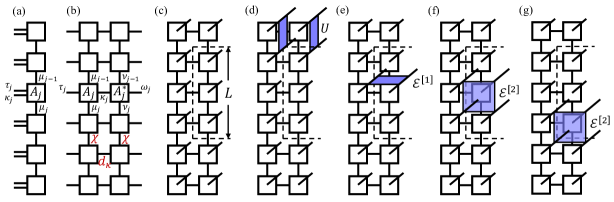
Figure 1: The implementation of a quantum circuit on a mixed state. (a) The purified state of an LPDO. (b) Mixed state in its LPDO representation. (c) The corresponding supervector in its PEPS representation. (d) The implementation of a two-qubit gate. (e) The implementation of single-qubit noise. (f-g) The implementation of two-qubit noise.

To gain a comprehensive understanding of the LPDO structure, especially the role played by inner indices, we start from an MPS shown in Fig. 1 (a) with two physical indices at each site

$$\ket{\psi}=\sum_{\{\bm{\tau},\bm{\kappa}\}}\sum_{\{\bm{\mu}\}}\prod_{j=1}^{N}[A_{j}]^{\tau_{j},\kappa_{j}}_{\mu_{j-1},\mu_{j}}\ket{\tau_{1},\kappa_{1},\cdots,\tau_{N},\kappa_{N}},$$ (1)

where $\bm{\mu}$ denote virtual indices and $\bm{\kappa}$ represent Kraus indices. Tracing out all the Kraus indices yields the following mixed state

$$\begin{aligned} \rho={\rm Tr}_{\kappa}{\left[\ket{\psi}\bra{\psi}\right]}=&\sum_{\{\bm{\tau},\bm{\omega}\}}\sum_{\{\bm{\mu},\bm{\nu},\bm{\kappa}\}}\prod_{j=1}^{N}[A_{j}]^{\tau_{j},\kappa_{j}}_{\mu_{j-1},\mu_{j}}[A_{j}^{*}]^{\omega_{j},\kappa_{j}}_{\nu_{j-1},\nu_{j}}\\ &\ket{\tau_{1},\cdots,\tau_{N}}\bra{\omega_{1},\cdots,\omega_{N}},\end{aligned}$$ (2)

as depicted in Fig. 1 (b). In this sense, $\ket{\psi}$ serves to purify $\rho$, where an ancillary degree of freedom (the Kraus index) is attached to the physical index via a local tensor at each site. Therefore, LPDO provides a locally purified form for the density matrix, from which it derives its name. Similar to the well-established connection between the locality of interaction and the efficient MPS representation, local purification also requires locality between the system and environment, where system qubits only interact with adjacent ancillae.

From the purification perspective, we can see that $d_{\kappa}$ equal to the physical bond dimension $d_{p}$ is sufficient to represent any mixed state exactly. However, this requires a large $\chi$ that may grow exponentially with the system size. Nevertheless, choosing a larger $d_{\kappa}$ can reduce $\chi$ and overall complexity while maintaining accuracy. This implies that these two inner indices should be considered together, as illustrated in the following discussion.

PEPS representation for an LPDO.— A general mixed state allows for an eigenvalue decomposition as

$$\rho=\sum_{k}{\lambda_{k}\ket{\psi_{k}}\bra{\psi_{k}}}~{},$$ (3)

which naturally corresponds to an unnormalized supervector in the double space

$$|\rho\rangle\!\rangle=\sum_{k}{\lambda_{k}\ket{\psi_{k}}\otimes\ket{\psi_{k}}}~{}.$$ (4)

In this sense, a one-dimensional (1D) mixed state with $N$ qubits is converted into a quasi-1D system of size $2\times N$.

For example, a density operator $\rho$ represented by an LPDO can be viewed as a $2\times N$ ladder projected entangled-pair state (PEPS), as shown in Fig. 1 (c). Therefore, if the quantum state defined in Eq. (4) satisfies the entanglement area law, the original mixed state in Eq. (3) can be represented by an LPDO.

Entanglement dynamics in noisy quantum circuits.—

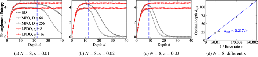
Figure 2: (a-c) Entanglement entropy dynamics of noisy quantum circuits with $N=8$ and different $\varepsilon$ for ED, MPO with different $D$, and LPDO with $d_{\kappa}=2$ and different $\chi$. The blue dashed lines indicate the positions where MPO and LPDO simulations deviate, consistent with the ‘optimal depth’ [22]. (d) The ‘optimal depth’ for $N=8$ and different $\varepsilon$ fitted as $d\sim 0.217/\varepsilon$.

Here, we conduct a systematic investigation into the entanglement dynamics in a general noisy quantum circuit. As depicted in Fig. 1 (c), a subsystem of size $1\times L$ is divided from the entire PEPS, requiring a $O(L)$ scaling of the entanglement entropy between two subsystems to ensure an efficient PEPS representation. Therefore, it is important to study how these basic components that make up a noisy quantum circuit, namely unitary gates and noise channels, contribute to this bipartite entanglement measure. In particular, to obtain a reasonable estimate for the entanglement entropy $S=-\sum_{k}{s_{k}^{2}\ln{s_{k}^{2}}}$, the corresponding Schmidt weights need to be normalized as $\sum_{k}s_{k}^{2}=1$, which requires normalization of the supervector as $\langle\!\langle\rho|\rho\rangle\!\rangle={\rm Tr}{\left[\rho^{2}\right]}=1$.

It is obvious that a single-qubit gate will not affect any entanglement structure, so we proceed directly to the analysis of two-qubit gates.

1. Two-qubit unitary gates. Consider a conventional two-qubit gate applied to the mixed state as $U\rho U^{\dagger}$, where the corresponding transformation in the supervector is expressed as

$$U\otimes\overline{U}|\rho\rangle\!\rangle.$$ (5)

The only scenario for a two-qubit gate to change the entanglement of $|\rho\rangle\!\rangle$ is when the unitary crosses the division line, as illustrated in Fig. 1 (d). Suppose that the potential capacity for the unitary to generate entanglement in a normal quantum state is denoted as $C_{U}$, (e.g., $C_{U}$ for a CNOT gate is $C_{U}=\ln{2}$), then it can be directly shown that the entanglement increase of the supervector also follows the conventional rule. Consequently, if a layer of two-qubit gates is applied to the quantum state, with one gate acting on each nearest-neighbor pair, the entanglement entropy of the supervector across the division line shown in Fig. 1 (d) satisfies that

$$\Delta S\leq 2C_{U}.$$ (6)

2. Single-qubit noise. General quantum noise can be expanded in its operator-sum representation as follows

$$\mathcal{E}^{[1]}\left(\rho\right)=\sum_{k}E_{k}\rho E_{k}^{\dagger}.$$ (7)

As illustrated in the following example, such a single-qubit noise channel (Fig. 1 (e)) exhibits little difference from the two-qubit unitary gate discussed before from the PEPS perspective. Here we consider a single-qubit Pauli error as an example, $\mathcal{E}\left(\rho\right)=(1-\varepsilon)\rho+\varepsilon\sigma^{x}\rho\sigma^{x}$, whose effect on the supervector is given by

$$\mathcal{E}|\rho\rangle\!\rangle\propto(1-\varepsilon)|\rho\rangle\!\rangle+\varepsilon\sigma^{x}\otimes\overline{\sigma^{x}}|\rho\rangle\!\rangle.$$ (8)

This just behaves like an entangled gate (non-unitary though) applied across two subsystems, a fact that can be also inferred from the similarity between Fig. 1 (d) and (e). As a result, if each qubit undergoes a single-qubit noise, we expect that the change in entanglement entropy satisfies that

$$\Delta S\leq LC_{\mathcal{E}}^{[1]},$$ (9)

where $C_{\mathcal{E}}^{[1]}\sim a\varepsilon$ with $a$ being a constant of the order $O(1)$.

3. Two-qubit noise. Finally, we examine the effect of a two-qubit noise channel on supervector entanglement. We again consider a two-qubit Pauli noise as an illustrative example, i.e., $\mathcal{E}^{[2]}(\rho)=(1-\varepsilon)\rho+\varepsilon\left(\sigma^{x}_{i}\otimes\sigma^{x}_{j}\right)\rho\left(\sigma^{x}_{i}\otimes\sigma^{x}_{j}\right)$ for adjacent sites $\braket{i,j}$. The corresponding transformation of the supervector is

$$\mathcal{E}|\rho\rangle\!\rangle\propto(1-\varepsilon)|\rho\rangle\!\rangle+\varepsilon\sigma^{x}_{i}\otimes\sigma^{x}_{j}\otimes\overline{\sigma^{x}_{i}}\otimes\overline{\sigma^{x}_{j}}|\rho\rangle\!\rangle,$$ (10)

where two cases arise as shown in Fig. 1 (f) and (g). In Fig. 1 (f), the two qubits that support the noise channel lie within the divided subsystem, while the pair $\braket{i,j}$ crosses the division in Fig. 1 (g). Nevertheless, it can be readily verified that these two cases will lead to the same increase in the entanglement entropy of $|\rho\rangle\!\rangle$ with $\Delta S\leq C_{\mathcal{E}}^{[2]}$. This means that a layer of two-qubit noise will induce an entanglement increase of

$$\Delta S\leq(L+1)C_{\mathcal{E}}^{[2]}.$$ (11)

Similarly, $C_{\mathcal{E}}^{[2]}\sim b\varepsilon$ with $b$ being a constant of the order $O(1)$.

In summary, for a typical quantum circuit with single-qubit gates in the odd layers and two-qubit gates in the even layers, along with single-qubit and two-qubit noise respectively, the entanglement growth under circuit depth $d$ can be estimated as

$$\Delta S\leq\frac{d}{2}(2C_{U}+LC_{\mathcal{E}}^{[1]}+(L+1)C_{\mathcal{E}}^{[2]})=O(d\varepsilon L).$$ (12)

Consequently, the supervector $|\rho\rangle\!\rangle$ for a mixed state generated from a noisy circuit with depth scaling lower than $d\sim\varepsilon^{-1}$ satisfies $S\lesssim O(L)$. This depth scaling ensures an efficient PEPS representation for $|\rho\rangle\!\rangle$, and thus an efficient LPDO representation for $\rho$. In other words, we expect a failure of the LPDO simulation when the circuit is deeper than the scaling behavior $d\sim\varepsilon^{-1}$, as demonstrated in the following numerical experiments.

Numerical simulations of noisy quantum circuits.—

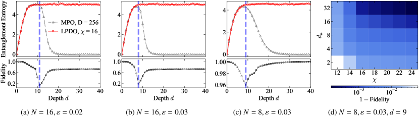
Figure 3: Fidelity for projection from an MPO to an LPDO compared with entanglement entropy dynamics simulated by both structures. (a-c) The upper panels show the entanglement entropy for noisy circuits with different $N$ and different $\varepsilon$. The lower panels show the fidelity of projecting an MPO with $D=256$ onto an LPDO with $\chi=16$ and $d_{\kappa}=2$. The blue dashed line indicates the position of minimum fidelity. (d) Projection from an MPO with $D=256$ generated from noisy circuits with $N=8$, ${\rm depth}=9$, and $\varepsilon=0.03$ to an LPDO with different $\chi$ and $d_{\kappa}$.

In our numerical simulations, we use brick-wall circuits with Haar-random two-qubit gates [53, 54, 55] accompanied by two-qubit depolarizing noise—a common circuit structure in related works.

Initially, we focus on systems with $N=8$ qubits whose entire dynamics can be exactly simulated as a benchmark. The bipartite (divided at half of the chain) EE of the supervector $|\rho\rangle\!\rangle$ calculated by exact diagonalization (ED), matrix product operator (MPO) simulation, and the LPDO simulation are compared in Fig. 2 for different two-qubit error rates $\varepsilon$. The truncation of MPO follows the conventional method [22], while we modify the LPDO truncation method to enhance the accuracy and robustness, as illustrated in Supplemental Material [55]. First, we observe an increasing-decreasing trend of EE from ED simulation, which divides the entire dynamics into two regions: (1) a quantum region where quantum entanglement gradually accumulates, potentially offering quantum advantages for systems with much larger sizes; (2) a classical region dominated by noise effects, leading to highly depolarized and mixed systems. consistent with the numerical results in recent works [22, 52, 51].

Second, the MPO simulation with a larger $D$ better approximates the dynamics as expected. However, even with a substantial $D=144$, especially considering that the system size is only $N=8$ for which $D=256$ would be enough for an exact representation, there is still a noticeable deviation from the exact results, limiting the application of MPO to simulating large-scale noisy quantum computers. On the contrary, LPDO allows an accurate description of EE dynamics with a relatively small $d_{\kappa}$ in the quantum region. Specifically, an LPDO with $\chi$ and $d_{\kappa}=2$ exhibits expressive power comparable to that of an MPO with $D=\chi^{2}$ under the condition of weak noise, while the former structure consumes significantly less computational resources.

However, we must also point out that when the circuit transitions into the classical region, an LPDO can no longer accurately capture the exact trajectories because of the large decoherence effects. The occurrence of this failure coincides with the crossover point between the quantum and classical regions, where the circuit EE starts to decrease from its maximal value. This ‘optimal depth’ for reaching maximal entanglement, as defined in previous numerical works [22] and marked by blue dashed lines in Fig. 2 (a-c), has been fitted as $d_{\rm opt}\sim 0.217/\varepsilon$ in Fig. 2 (d), validating our theoretical analysis and prediction near Eq. (12). Moreover, the consistency between these two types of critical points (the failure of LPDO and the maximal EE) implies the existence of much more interesting properties in this critical region. In the subsequent analysis, we aim to explore the properties of these dynamical critical points and explain the limitations of the LPDO simulation in this context.

Projection to an LPDO.— To address the problem of whether an LPDO is sufficient to represent the noisy quantum state near the critical region, we propose a gradient descent algorithm to project an MPO onto an LPDO. To be more specific, we aim to optimize the following loss function

$$\Theta=\left|\left|\rho-\rho^{\prime}\right|\right|_{F}^{2}={\rm Tr}{\left[\rho^{2}+\rho^{\prime 2}-2\rho\rho^{\prime}\right]},$$ (13)

where $\rho$ represents the original MPO and $\rho\prime$ denotes the approximated LPDO. To obtain an approximated LPDO $\rho^{\prime}$ with minimal loss $\Theta$, one needs to evaluate the gradient with respect to each tensor as

$$\frac{\partial\Theta}{\partial A_{j}^{*}}=2{\rm Tr}{\left[\left(\rho^{\prime}-\rho\right)\frac{\partial\rho^{\prime}}{{\partial A_{j}^{*}}}\right]},$$ (14)

which can be analytically derived and efficiently computed in $O(N)$ time by caching the tensor environment [56, 27, 55]. Importantly, this method also applies to the truncation of an MPO or LPDO, which can be viewed as a projection from an MPO/LPDO with a larger bond dimension to another one with a smaller bond dimension. Fig. 3 (a-b) plot the projection fidelity from the simulated MPO with $D=256$ to an LPDO with fixed $\chi=16$ and $d_{\kappa}=2$ for different $N$ and $\varepsilon$, along with the directly simulated LPDO dynamics with the same $d_{\kappa}$ and $\chi$. The results clearly reveal minimal fidelity at the critical point where the EE estimated by MPO and LPDO deviate, explaining the failure of LPDO simulation in that region.

Meanwhile, projection fidelity appears unsatisfactory throughout the dynamics of $N=16$, which we attribute to the inaccurate MPO representation with only $D=256$. The truncation of MPO during the simulation introduces non-Hermitian and non-positive parts, breaking several physical conditions of a valid density matrix. For systems with only $N=8$, where an exact MPO representation is available, the overall trend of the projection fidelity is quite similar, but the values are much higher when comparing Fig. 3(b) and (c).

Finally, we compare the expressive capacity of LPDO with different $\chi$ and $d_{\kappa}$ for noisy quantum states. To avoid the above issue of an inaccurate MPO representation, we adopt $N=8$ and directly implement the projection from the exact density matrices generated from the noisy circuits with $\varepsilon=0.03$ and $d=9$ to LPDO, just at the critical point between the quantum and classical regions. From the projection fidelity shown in Fig. 3 (d), we observe that, e.g., an LPDO with $\chi=24$ and only $d_{\kappa}=4$ can possess a representative power similar to that of an LPDO with $\chi=14$ but much larger $d_{\kappa}$, at least for these quantum states generated from typical noisy quantum circuits of interest. This implies that the difference between virtual indices and Kraus indices is not absolute, and a unified scheme to treat them according to our proposal is reasonable. On the other hand, it suggests that in a critical region where quantum entanglement and noise effects coexist, an effective strategy is to start by choosing a large $\chi$ to capture both classical and quantum correlations between different sites, and then gradually increasing $d_{\kappa}$ to refine the approximation and approach the target state. This reveals the complementary roles played by these two indices in achieving an accurate representation of noisy quantum systems in such challenging regimes.

Conclusion and discussion.— In conclusion, our investigation into the simulation of open quantum systems through the LPDO representation has clarified its capacity and limitations when dealing with the dynamics of noisy quantum circuits. We introduce a unified framework to understand two internal indices in LPDO, aiming to bridge the gap for their physical interpretation, which has proven valuable in providing an intuitive understanding of the entanglement structure in many-body mixed states. We also employ a gradient descent algorithm to project MPOs onto LPDOs, which has demonstrated its own effectiveness and certified the LPDO simulation in the quantum region where quantum entanglement prevails. However, the critical point between the quantum and classical regions remains a challenge for LPDO simulation, as evidenced by the divergence in EE from exact results and a minimal fidelity for the projection.

Several avenues for future research emerge. For example, further exploration and characterization of the interplay between noise effects and quantum entanglement, especially at the crossover between quantum and classical regions, are essential [57]. Furthermore, the possible connections to these measurement or noise-induced phase transitions [58, 59, 60, 61, 62, 63] or other dynamical phase transitions [64, 65, 66, 67, 68] are also interesting. In summary, the challenges and opportunities identified in this study provide a foundation for further research into the efficient representation and simulation of noisy quantum states, offering potential advances in quantum information processing and quantum computing.

Supplemental Material

In this supplemental material, we provide more details on the truncation method of LPDO, the conversion between MPO and LPDO, and the circuit configuration in numerical simulations.

Appendix S-1 The truncation method of LPDO

The LPDO truncation in previous work [43, 23] is done by directly applying the singular value decomposition (SVD) to local tensors and truncating the singular values for the Kraus indices and virtual indices in sequence. For instance, all Kraus indices were first truncated via local SVD without considering the tensor environment, and then the virtual indices were truncated site by site in the canonical form in Ref. [23]. Such a sequence for different indices and the neglect of the environment when truncating $d_{\kappa}$ limit accuracy and robustness. Here, we introduce a modified three-step compression scheme, where a site-by-site QR and LQ decomposition is first performed to obtain the gauge transformations $L_{i}$ and $R_{i}$ on each virtual index. Next, the projectors for Kraus indices and virtual indices are calculated respectively with the standard SVD compression. Finally, all projectors are applied simultaneously to complete the truncation of LPDO.

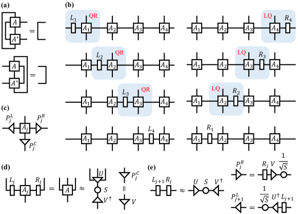
Figure S1: Truncation of LPDO. (a) Left and right canonical conditions. (b) Site-by-site QR and LQ decomposition. (c) Projectors for truncation. (d) Construction of Kraus-index projector. (e) Construction of virtual-index projector.

The canonical form of an LPDO is naturally generalized from that of an MPS, where both physical indices and Kraus indices are traced when calculating the environment, as shown in Fig. S1 (a). First, we implement a left-to-right QR decomposition in Fig. S1 (b) to obtain the gauge matrices $L_{i}$ for the left-canonical form, where $L_{1}=[1]$, a $1\times 1$ identity matrix. Similarly, a left-to-right LQ decomposition starts from $R_{N}=[1]$ is performed to calculate $R_{i}$ for the right-canonical form. All $L_{i}$ and $R_{i}$ are stored for later construction of projectors. Next, we construct the projectors for both virtual indices $P_{j}^{L},P_{j}^{R}$, and Kraus index $P_{j}^{C}$ for each local tensor $A_{j}$ in Fig. S1 (c) inspired from Ref. [69]. For the Kraus index, we absorb the gauge on virtual indices $L_{j}$ and $R_{j}$ into $A_{j}$ leading to $\tilde{A}_{j}$ and perform SVD along the vertical direction $\tilde{A}_{j}\approx USV^{\dagger}$, as shown in Fig. 3 (d). The local projector is constructed as $P_{j}^{C}=V$. It can be easily verified that

$$\tilde{A}_{j}P_{j}^{C}P^{C\dagger}_{j}\tilde{A}_{j}^{\dagger}\approx USV^{\dagger}VV^{\dagger}VSU^{\dagger}=US^{2}U^{\dagger},$$ (S1)

which does realize the compression of the Kraus index. Regarding the virtual index, we contract the gauge from two sides and implement SVD, i.e., $L_{j+1}R_{j}\approx USV^{\dagger}$, and construct the corresponding projectors in Fig. S1 (e), namely $P_{j}^{R}=R_{j}V\frac{1}{\sqrt{S}}$ and $P_{j+1}^{L}=\frac{1}{\sqrt{S}}U^{\dagger}L_{j+1}$. Such projectors satisfy

$$P_{j}^{R}P_{j+1}^{L}=R_{j}V\frac{1}{\sqrt{S}}\frac{1}{\sqrt{S}}U^{\dagger}L_{j+1}\approx R_{j}\left(L_{j+1}R_{j}\right)^{-1}L_{j+1}=I.$$ (S2)

We must emphasize that in this process, the Kraus index has not been truncated yet in order to maintain the most accurate tensor environment. Finally, all projectors $P_{j}^{C}$, $P_{j}^{L}$, and $P_{j}^{L}$ constructed before are simultaneously applied to the local tensor of each site, resulting in a truncated LPDO with smaller $\chi$ and $d_{\kappa}$.

Appendix S-2 The conversion between MPO and LPDO

The LPDO structure in Fig. S2 (b) is proposed in Ref. [40] as a natural generation of MPS to represent mixed states

$$\rho=\sum_{\{\bm{\mu},\bm{\nu}\}}\sum_{\{\bm{\kappa}\}}\prod_{j=1}^{N}[A_{j}]^{\tau_{j},\kappa_{j}}_{\mu_{j-1},\mu_{j}}[A_{j}^{*}]^{\omega_{j},\kappa_{j}}_{\nu_{j-1},\nu_{j}}\ket{\tau_{1},\cdots,\tau_{N}}\bra{\omega_{1},\cdots,\omega_{N}},$$ (S3)

where $\bm{\kappa}$ are Kraus indices that represent the environment (or ancillae) to be traced out. Notably, an LPDO is guaranteed to be Hermitian and semidefinite positive by design due to its quadratic form with respect to local tensors.

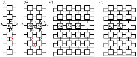
Figure S2: MPO and LPDO representation for mixed states. (a) A mixed state represented by an MPO. (b) A mixed state represented by an LPDO. (c) The environment for ${\rm Tr}{\left[\rho^{\prime}\left(\partial\rho^{\prime}/\partial A_{j}^{*}\right)\right]}$. (d) The environment for ${\rm Tr}{\left[\rho\left(\partial\rho^{\prime}/\partial A_{j}^{*}\right)\right]}$.

Another commonly adopted TN member to represent a mixed state is the MPO shown in Fig. S2 (a)

$$\rho=\sum_{\{\bm{\sigma}\}}\prod_{j=1}^{N}[B_{j}]^{\tau_{j},\omega_{j}}_{\sigma_{j-1},\sigma_{j}}\ket{\tau_{1},\cdots,\tau_{N}}\bra{\omega_{1},\cdots,\omega_{N}},$$ (S4)

which can be obtained by directly contracting the two local tensors at each site, i.e.,

$$[B_{j}]^{\tau_{j},\omega_{j}}_{\sigma_{j-1},\sigma_{j}}=\sum_{\kappa_{j}}[A_{j}]^{\tau_{j},\kappa_{j}}_{\mu_{j-1},\mu_{j}}[A_{j}^{*}]^{\omega_{j},\kappa_{j}}_{\nu_{j-1},\nu_{j}}$$ (S5)

with $\sigma_{j}=\left\{\mu_{j},\nu_{j}\right\}$. In other words, the bond dimension $D$ of an MPO is typically much larger than $\chi$ of an LPDO in the weak-noise region, In the pure-state limit, an MPS (which corresponds to an LPDO with $d_{\kappa}=1$) with $\chi$ corresponds to an MPO with $D=\chi^{2}$. In addition, it is hard to directly impose the constraints of Hermicity and positivity on the construction of an MPO, and to our knowledge there has been no approach to recover a legible density matrix from a general MPO so far. Therefore, more and more efforts have been put into the LPDO representation and simulation for open quantum systems.

We have introduced an approach to project any MPO to an LPDO with given $\chi$ and $d_{\kappa}$, or more precisely, to find the LPDO with the smallest distance from the target MPO defined by the Frobenius norm in Eq. (13) of the main text. The gradient of each tensor is analytically shown in Fig. S2 (c-d), corresponding to the two terms in Eq. (14) in the main text, respectively. In each iteration step, We update the local tensor $A_{j}$ according to the following rule

$$A_{j}\rightarrow A_{j}-\eta\frac{\partial\Theta}{\partial A_{j}^{*}}$$ (S6)

where $\eta$ is the learning rate, automatically adjusted using the Adam optimizer [70]. The hyperparameters in the Adam optimizer are set as $\xi_{1}=\xi_{2}=0.8$ and $\epsilon=10^{-8}$ throughout the numerical simulations in this work.

Appendix S-3 Circuit configuration in numerical simulations

In the numerical simulations, we use the test circuit shown in Fig. S3, as commonly adopted in various quantum computing tasks [55]. In this circuit, each layer is a tensor product of two-qubit Haar-random gates with a staggered arrangement between adjacent layers. To be more specific, each local gate $U$ is drawn randomly and independently of all the others from the uniform distribution on the unitary group $U(4\times 4)$ [54]. We introduce two-qubit depolarizing noise channels after each gate, defined as

$$\begin{aligned} \mathcal{E}^{[2]}\left(\rho\right)=\left(1-\frac{16}{15}\varepsilon\right)\rho+\frac{1}{15}\varepsilon\sum_{i,j=0}^{3}\left(\sigma_{i}\otimes\sigma_{j}\right)\rho\left(\sigma_{i}\otimes\sigma_{j}\right),\end{aligned}$$ (S7)

where $\varepsilon$ is the two-qubit error rate, typically at the order of $10^{-2}$ for state-of-the-art quantum hardware.

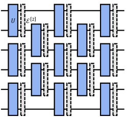
Figure S3: The circuit configuration. Two-qubit gates $U$ follow the random Haar measure, followed by two-qubit depolarizing noise $\mathcal{E}^{[2]}$.

Appendix S-4