Convergence Rates for Stochastic Approximation:
Biased Noise with Unbounded Variance, and Applications

Abstract

The Stochastic Approximation (SA) algorithm introduced by Robbins and Monro in 1951 has been a standard method for solving equations of the form ${\bf f}({\boldsymbol{\theta}})={\bf 0}$, when only noisy measurements of ${\bf f}(\cdot)$ are available. If ${\bf f}({\boldsymbol{\theta}})=\nabla J({\boldsymbol{\theta}})$ for some function $J(\cdot)$, then SA can also be used to find a stationary point of $J(\cdot)$. At each time $t$, the current guess ${\boldsymbol{\theta}}_{t}$ is updated to ${\boldsymbol{\theta}}_{t+1}$ using a noisy measurement of the form ${\bf f}({\boldsymbol{\theta}}_{t})+{\boldsymbol{\xi}}_{t+1}$. In much of the literature, it is assumed that the error term ${\boldsymbol{\xi}}_{t+1}$ has zero conditional mean, and that its conditional variance is bounded as a function of $t$ (though not necessarily with respect to ${\boldsymbol{\theta}}_{t}$). Over the years, SA has been applied to a variety of areas, out of which the focus in this paper is on convex and nonconvex optimization. As it turns out, in these applications, the above-mentioned assumptions on the measurement error do not always hold. In zero-order methods, the error neither has zero mean nor bounded conditional variance. In the present paper, we extend SA theory to encompass errors with nonzero conditional mean and/or unbounded conditional variance. In addition, we derive estimates for the rate of convergence of the algorithm, and compute the “optimal step size sequences” to maximize the estimated rate of convergence.

1 Introduction

1.1 Brief Literature Review

Since its introduction in 1951 in [34], the Stochastic Approximation (SA) algorithm has become one of the standard probabilistic methods for solving equations of the form ${\bf f}({\boldsymbol{\theta}})={\bf 0}$, when only noisy measurements of ${\bf f}(\cdot)$ are available. Over the years, SA has been applied to a variety of areas, including the two topics addressed here, namely: convex and nonconvex optimization, and Reinforcement Learning (RL). In this paper, we present several new directions and results in the theory of stochastic approxiation (SA), along with their applications to optimization. Some possible applications to RL are indicated in the Conclusions section.

Suppose ${\bf f}:{\mathbb{R}}^{d}\rightarrow{\mathbb{R}}^{d}$ is some function, and it is desired to find a solution ${\boldsymbol{\theta}}^{*}$ to the equation ${\bf f}({\boldsymbol{\theta}}^{*})={\bf 0}$. The stochastic approximation (SA) algorithm, introduced in [34], addresses the situation where the only information available is a noise-corrupted measurement of ${\bf f}({\boldsymbol{\theta}}_{t})$, in the form ${\bf f}({\boldsymbol{\theta}}_{t})+{\boldsymbol{\xi}}_{t+1}$, where ${\boldsymbol{\xi}}_{t+1}$ is the error term. If ${\bf g}:{\mathbb{R}}^{d}\rightarrow{\mathbb{R}}^{d}$ and it is desired to find a fixed point of this map, then this is the same as solving ${\bf f}({\boldsymbol{\theta}}^{*})={\bf 0}$, where ${\bf f}({\boldsymbol{\theta}}):={\bf g}({\boldsymbol{\theta}})-{\boldsymbol{\theta}}$. Finally, if $J:{\mathbb{R}}^{d}\rightarrow{\mathbb{R}}$ is a ${\mathcal{C}}^{1}$ function and it is desired to find a stationary point of $J(\cdot)$, then the problem is to find a solution to $\nabla J({\boldsymbol{\theta}}^{*})={\bf 0}$.

Suppose the problem is one of finding a solution to ${\bf f}({\boldsymbol{\theta}}^{*})={\bf 0}$. The canonical step in the SA algorithm is to update ${\boldsymbol{\theta}}_{t}$ to ${\boldsymbol{\theta}}_{t+1}$ via

$${\boldsymbol{\theta}}_{t+1}={\boldsymbol{\theta}}_{t}+\alpha_{t}[{\bf f}({\boldsymbol{\theta}}_{t})+{\boldsymbol{\xi}}_{t+1}],$$ (1)

where $\alpha_{t}$ is called the “step size.” If one wishes to find a fixed point of the map ${\bf g}(\cdot)$, then by defining ${\bf f}({\boldsymbol{\theta}})={\bf g}({\boldsymbol{\theta}})-{\boldsymbol{\theta}}$, one can apply the iteration (1), which now takes the form

$${\boldsymbol{\theta}}_{t+1}=(1-\alpha_{t}){\boldsymbol{\theta}}_{t}+\alpha_{t}[{\bf g}({\boldsymbol{\theta}}_{t})+{\boldsymbol{\xi}}_{t+1}].$$ (2)

Finally, if it is desired to find a stationary point of a ${\mathcal{C}}^{1}$-map $J(\cdot)$, the iteration becomes

$${\boldsymbol{\theta}}_{t+1}={\boldsymbol{\theta}}_{t}-\alpha_{t}{\bf h}_{t+1},$$ (3)

where ${\bf h}_{t+1}$ is a noisy approximation to $\nabla J({\boldsymbol{\theta}}_{t})$. Equations (1), (2) and (3) are the most commonly used variants of SA.

Leaving aside the assumptions on the functions ${\bf f},{\bf g},J$ as the case might be, different implementations of the algorithm differ in the choice of the step size sequence, and the assumptions on the error ${\boldsymbol{\xi}}_{t+1}$. In this brief review, we will attempt to describe the literature that is most relevant to the present paper. In order to describe work concisely, we introduce some notation. Let ${\boldsymbol{\theta}}_{0}^{t}$ denote $({\boldsymbol{\theta}}_{0},\cdots,{\boldsymbol{\theta}}_{t})$, and similarly let ${\boldsymbol{\xi}}_{1}^{t}$ denote ${\boldsymbol{\xi}}_{1},\cdots,{\boldsymbol{\xi}}_{t}$; note that there is no ${\boldsymbol{\xi}}_{0}$. The initial guess ${\boldsymbol{\theta}}_{0}$ in SA can be either deterministic or random. Let ${\mathcal{F}}_{t}$ denote the $\sigma$-algebra generated by ${\boldsymbol{\theta}}_{0},{\boldsymbol{\xi}}_{1}^{t}$. Let ${\mathcal{M}}({\mathcal{F}}_{t})$ denote the set of functions that are measurable with respect to ${\mathcal{F}}_{t}$. Then it is clear that ${\boldsymbol{\theta}}_{t}\in{\mathcal{M}}({\mathcal{F}}_{t})$ for all $t\geq 1$. For an ${\mathbb{R}}^{d}$-valued random variable $X$, let $E_{t}(X)$ denote the conditional expectation $E(X|{\mathcal{F}}_{t})$, and let $CV_{t}(X)$ denote its conditional variance defined by

$$CV_{t}(X)=E_{t}(\|X-E_{t}(X)\|_{2}^{2}).$$ (4)

We begin with the classical results. In [34] which introduced the SA algorithm for the scalar case where $d=1$. However, we state it for the multidimensional case. In this formulation, the error ${\boldsymbol{\xi}}_{t+1}$ is assumed to satisfy the following assumptions (though this notation is not used in that paper)

$$E_{t}({\boldsymbol{\xi}}_{t+1})={\bf 0},CV_{t}({\boldsymbol{\xi}}_{t+1})\leq M^{2}$$ (5)

for some finite constant $M$. The first assumption implies that $\{{\boldsymbol{\xi}}_{t+1}\}$ is a martingale difference sequence, and also that ${\bf f}({\boldsymbol{\theta}}_{t})+{\boldsymbol{\xi}}_{t+1}$ is an unbiased measurement of ${\bf f}({\boldsymbol{\theta}}_{t})$. The second assumption means that the conditional variance of the error is globally bounded, both as a function of ${\boldsymbol{\theta}}_{t}$ and as a function of $t$. With the assumptions in (6), along with some assumptions on the function ${\bf f}(\cdot)$, it is shown in [34] that ${\boldsymbol{\theta}}_{t}$ converges to a solution of ${\bf f}({\boldsymbol{\theta}}^{*})={\bf 0}$, provided the step size sequence satisfies the Robbins-Monro (RM) conditions

$$\sum_{t=0}^{\infty}\alpha_{t}^{2}<\infty,\sum_{t=0}^{\infty}\alpha_{t}=\infty.$$ (6)

This approach was extended in [19] to finding a stationary point of a ${\mathcal{C}}^{1}$ function $J:{\mathbb{R}}\rightarrow{\mathbb{R}}$, that is, a solution to $\nabla J({\boldsymbol{\theta}})={\bf 0}$, using an approximate gradient of $J(\cdot)$. The specific formulation used in [19] is

$$h_{t+1}:=\frac{J(\theta_{t}+c_{t}\Delta+\xi_{t+1}^{+})-J(\theta_{t}-c_{t}\Delta+\xi_{t+1}^{-})}{2c_{t}}\approx\nabla J(\theta_{t}).$$ (7)

where $c_{t}$ is called the increment, $\Delta$ is some fixed number, and $\xi_{t+1}^{+}$, $\xi_{t+1}^{-}$ are the measurement errors. This terminology “increment” is not standard but is used here. In order to make the expression a better and better approximation to the true $\nabla J({\boldsymbol{\theta}}_{t})$, the increment $c_{t}$ must approach zero as $t\rightarrow\infty$. This approach was extended to the multidimensional case in [5]. There are several ways to extend (7) to the multivariate case, and these are discussed in Section 4. Equation (7) is one example of (3). Let ${\bf h}_{t+1}$ denote the (negative of the) search direction, however chosen, and define

$${\bf z}_{t}=E_{t}({\bf h}_{t+1}),{\bf x}_{t}={\bf z}_{t}-\nabla J({\boldsymbol{\theta}}_{t}),{\boldsymbol{\zeta}}_{t+1}={\bf h}_{t+1}-{\bf z}_{t}.$$ (8)

In all the ways in which ${\bf h}_{t+1}$ is defined in Section 4, the error term satisfies

$$\|E_{t}({\boldsymbol{\zeta}}_{t+1})\|_{2}\leq Kc_{t},CV_{t}({\boldsymbol{\zeta}}_{t+1})\leq M^{2}/c_{t}^{2},$$ (9)

for suitable constants $K,M$. In other words, neither of the two assumptions in (5) is satisfied: The estimate of $\nabla J({\boldsymbol{\theta}}_{t})$ is biased, and the variance is unbounded as a function of $t$, though it is bounded as a function of ${\boldsymbol{\theta}}_{t}$ for each fixed $t$. In this case, for the scalar case, it was shown in [19] that ${\boldsymbol{\theta}}_{t}$ converges to a stationary point of $J(\cdot)$ if the Kiefer-Wolfwitz-Blum (KWB) conditions

$$c_{t}\rightarrow 0,\sum_{t=0}^{\infty}(\alpha_{t}^{2}/c_{t}^{2})<\infty,\sum_{t=0}^{\infty}\alpha_{t}c_{t}<\infty,\sum_{t=0}^{\infty}\alpha_{t}=\infty$$ (10)

are satisfied. In [5] it is shown that the same conditions also ensure convergence when $d>1$. Note that the conditions automatically imply the finiteness of the sum of $\alpha_{t}^{2}$.

Now we summarize subsequent results. It can be seen from Theorem 3 below that in the present paper, the error ${\boldsymbol{\xi}}_{t+1}$ is assumed to satisfy the following assumptions:

$$\|E_{t}({\boldsymbol{\xi}}_{t+1})\|_{2}\leq\mu_{t}(1+\|{\boldsymbol{\theta}}_{t}\|_{2}),$$ (11)

$$CV_{t}({\boldsymbol{\xi}}_{t+1})\leq M_{t}^{2}(1+\|{\boldsymbol{\theta}}_{t}\|_{2}^{2}),$$ (12)

where ${\boldsymbol{\theta}}_{t}$ is the current iteration. It can be seen that the above assumptions extend (9) in several ways. First, the conditional expectation is allowed to grow as an affine function of $\|{\boldsymbol{\theta}}_{t}\|_{2}$, for each fixed $t$. Second, the conditional variance is also allowed to grow as a quadratic function of $\|{\boldsymbol{\theta}}_{t}\|_{2}$, for each fixed $t$. Third, while the coefficient $\mu_{t}$ is required to approach zero, the coefficient $M_{t}$ can grow without bound as a function of $t$. We are not aware of any other paper that makes such general assumptions. However, there are several papers wherein the assumptions on ${\boldsymbol{\xi}}_{t+1}$ are intermediate between (5) and (9). We attempt to summarize a few of them next. For the benefit of the reader, we state the results using the notation of the present paper.

In [20], the author considers a recursion of the form

$${\boldsymbol{\theta}}_{t+1}={\boldsymbol{\theta}}_{t}-\alpha_{t}\nabla J({\boldsymbol{\theta}}_{t})+\alpha_{t}{\boldsymbol{\xi}}_{t+1}+\alpha_{t}{\boldsymbol{\beta}}_{t+1},$$

where ${\boldsymbol{\beta}}_{t}\rightarrow{\bf 0}$ as $t\rightarrow\infty$. Here, the sequence $\{{\boldsymbol{\xi}}_{t+1}\}$ is not assumed to be a martingale difference sequence. Rather, it is assumed to satisfy a different set of conditions, referred to as the Kushner-Clark conditions; see [20, A5]. It is then shown that if the error sequence $\{{\boldsymbol{\xi}}_{t+1}\}$ satisfies (5), i.e., is a martingale difference sequence, then Assumption (A5) holds. Essentially the same formulation is studied in [25]. The same formulation is also studied [6, Section 2.2], where (5) holds, and ${\boldsymbol{\beta}}_{t}\rightarrow{\bf 0}$ as $t\rightarrow\infty$. In [41], it is assumed only that $\limsup_{t}{\boldsymbol{\beta}}_{t}<\infty$. In all cases, it is shown that ${\boldsymbol{\theta}}_{t}$ converges to a solution of ${\bf f}({\boldsymbol{\theta}}^{*})={\bf 0}$, provided the iterations remain bounded almost surely. However, the assumption that $\beta_{t}\rightarrow 0$ as $t\rightarrow\infty$ may not, by itself, be sufficient to ensure that the iterations are bounded, as shown next.

Consider the deterministic scalar recursion

$$\theta_{t+1}=(1+\alpha_{t})\theta_{t}+\alpha_{t}\beta_{t},$$

where $\{\beta_{t}\}$ is a sequence of constants. Hence $\mu_{t}=|\beta_{t}|$ for all $i$. The closed-form solution to the above recursion is

$$\theta_{t}=\prod_{\tau=0}^{t}(1+\alpha_{t})\theta_{0}+\sum_{k=0}^{t-1}\left[\prod_{s=k}^{t-1}(1+\alpha_{s})\right]\alpha_{k}\beta_{k}.$$

Now let $\theta_{0}=0$ and suppose $\beta_{t}\geq 0$ for all $t$. Then it follows that

$$\theta_{t}=\sum_{k=0}^{t-1}\left[\prod_{s=k}^{t-1}(1+\alpha_{s})\right]\alpha_{t}\beta_{t}\geq\sum_{k=0}^{t-1}\alpha_{k}\beta_{t}.$$

Thus, even when the step size sequence $\{\alpha_{t}\}$ satisfies the standard Robbins-Monro conditions, it is possible to choose the sequence $\{\beta_{t}\}$ in such a manner that $\beta_{t}\rightarrow 0$ as $t\rightarrow\infty$, and yet

$$\sum_{t=0}^{\infty}\alpha_{t}\beta_{t}=\infty.$$

Thus, merely requiring that $\beta_{t}\rightarrow 0$ as $t\rightarrow\infty$ is not sufficient to ensure the boundedness of the iterations.

In all of the above references, the bound on $CV_{t}({\boldsymbol{\xi}}_{t+1})$ is as in (5). In [17], the authors study smooth convex optimization. They assume that the estimated gradient is unbiased, so that $\mu_{t}=0$ for all $t$. However, an analog of (12) is assumed to hold, which is referred to as “state-dependent noise.” See [17, Assumption (SN)]. In short, there is no paper wherein the assumptions on the error are as general as in (11) and (12).

In the present paper, all convergence proofs are based on the “supermartingale approach,” pioneered in [15, 35]. In contrast, in all the above references mentioned in the literature review, the convergence of the SA algorithm is proved using the so-called ODE method. This approach is based on the idea that, as $\alpha_{t}\rightarrow 0$, the sample paths of the stochastic process “converge” to the deterministic solutions of the associated ODE $\dot{{\boldsymbol{\theta}}}={\bf f}({\boldsymbol{\theta}})$. This approach is introduced in [20, 24, 10]. Book-length treatments of this approach can be found in [21, 22, 2, 6]. See also [26] for an excellent summary. In principle, the ODE method can cope with the situation where the equation ${\bf f}({\boldsymbol{\theta}}^{*})={\bf 0}$ has multiple solutions. The typical theorem in this approach states that if the iterations $\{{\boldsymbol{\theta}}_{t}\}$ remain bounded, then ${\boldsymbol{\theta}}_{t}$ approaches the solution set of the equation under study. In [7], for the first time, the boundedness of the iterations is a conclusion, not a hypothesis. The arguments in that paper, and its successors, are based on defining a mean flow equation

$$\dot{{\boldsymbol{\theta}}}=f_{\infty}({\boldsymbol{\theta}}),{\bf f}_{\infty}({\boldsymbol{\theta}}):=\lim_{r\rightarrow\infty}\frac{{\bf f}(r{\boldsymbol{\theta}})}{r}.$$

It is assumed that ${\bf f}(\cdot)$ is globally Lipschitz-continuous and that ${\bf 0}$ is a globally asymptotically stable equilibrium of ${\bf f}_{\infty}(\cdot)$. This implies that the equation under study has a unique solution, in effect negating one of the potential advantages of the ODE method. Also, it is easy to see that if ${\bf f}(\cdot)$ grows sublinearly, i.e.,

$$\lim_{\|{\boldsymbol{\theta}}\|\rightarrow\infty}\frac{\|{\bf f}({\boldsymbol{\theta}})\|}{\|{\boldsymbol{\theta}}\|}=0,$$

then ${\bf f}_{\infty}({\boldsymbol{\theta}})\equiv{\bf 0}$, so that the hypothesis of [7] can never be satisfied. In addition, when ${\bf f}(\cdot)$ is discontinuous, the limiting equation is not an ODE, but a differential inclusion; see for example [8]; this requires more subtle analysis. In contrast, the supermartingale method can cope with discontinuous ${\bf f}(\cdot)$ with no modifications.

In recent days, the approach of using approximate gradients to compute stationary points has been rediscovered several times, and is sometimes called a “zero-order” or “gradient-free” method. See [29] for a recent example. Interestingly, the paper [29] uses essentially the same method as in [37]. However, in [29], a bound on the rate of convergence is obtained, in contrast to [37].

Yet another recent development, which is popular when the dimension $d$ is large, is to compute (exactly or approximately) only a few components of $\nabla J({\boldsymbol{\theta}}_{t})$ at each $t$, and to update only the corresponding components of ${\boldsymbol{\theta}}_{t}$. This approach goes under a variety of names, such as Stochastic Gradient Descent (SGD), Block Stochastic Gradient Descent (BSGD) etc. Depending on the author, the evaluation of ${\bf J}({\boldsymbol{\theta}}_{t})$ and/or $\nabla J({\boldsymbol{\theta}}_{t})$ can either be exact or noisy. In the case where $\nabla J({\boldsymbol{\theta}}_{t})$ is available exactly, some survey papers such as [46, 42] provide very detailed analysis. However, the analysis is no longer applicable when the measurements are noisy. Moreover, though not always, the analysis is restricted to the case of convex objective functions. Still more recently, SA methods, specifically the Robbins-Siegmund theorem [35], have been used to establish the convergence of alternatives to the steepest descent method, such as the Heavy Ball method [23] or ADAM [1]. In [33], the convergence of the Heavy Ball method introduced in [31] is established under a variety of block-updating schemes. Since BSGD is a special case of the Heavy Ball method with the momentum parameter set to zero, these results also establish the convergence of BSGD under the same block updating schemes. This is but a very brief overview.

1.2 Contributions of the Paper

Now we describe briefly the contributions of the present paper.

• In the literature to date, the error ${\boldsymbol{\xi}}_{t+1}$ is assumed to satisfy one or both of the following assumptions:

  $$\|E_{t}({\boldsymbol{\xi}}_{t+1})\|_{2}\leq\mu_{t},CV_{t}({\boldsymbol{\xi}}_{t+1})\leq M^{2}(1+\|{\boldsymbol{\theta}}_{t}\|_{2}^{2}).$$

  In fact, we are not aware of any paper in which both of the above assumptions are permitted. Except for [17], the bound on $CV_{t}$ is just a constant $M^{2}$. In [17], the more general bound above is permitted, but $\mu_{t}$ is set to zero for all $t$. In contrast, we permit $\|E_{t}({\boldsymbol{\xi}}_{t+1})\|_{2}$ to be affine in $\|{\boldsymbol{\theta}}_{t}\|_{2}$, and $CV_{t}({\boldsymbol{\xi}}_{t+1})$ to be quadratic in $\|{\boldsymbol{\theta}}_{t}\|_{2}$. Moreover, $CV_{t}({\boldsymbol{\xi}}_{t+1})$ can also to be unbounded in $t$ for a fixed ${\boldsymbol{\theta}}_{t}$. The general assumption on $E_{t}({\boldsymbol{\xi}}_{t+1})$ is needed to analyze Markovian SA, while the generality on $CV_{t}({\boldsymbol{\xi}}_{t+1})$ is needed when approximate gradients are in gradient descent. In order to analyze this more general situation, we present a small extension of the classic theorem of Robbins-Siegmund [35], which may be of independent interest.

• We adapt an approach suggested in [23] and derive estimates of the rate at which the iterations converge to the desired limit.

• We extend both the convergence result and the rate estimate to the case of asynchronous updating, wherein the updating is governed by a binary-valued process. This permits us to study “synchronous” SA and “asynchronous” SA using a common framework.

• Using these results, we study the convergence of the stochastic gradient method in two situations: True gradient corrupted by additive noise, and approximate gradient (also known as zeroth-order methods) based on function measurements corrupted by noise. In the first case, it is known that the best achievable rate of convergence, even with noise-free gradient measurements, is $O(t^{-1})$. We show that, even in the presence of noise, it is possible to achieve convergence at the rate of $O(t^{-\lambda})$ for $\lambda$ arbitrarily close to one. In the case of using approximate gradients, it is known that, with noise-free function measurements, convergence takes place at the rate of $O(t^{-1/2})$. We show that, even with noisy function measurements, it is possible to achieve convergence at the rate of $O(t^{-\lambda})$ for $\lambda$ arbitrarily close to $1/3$. It is to be noted that our results apply not only to convex objective functions, but also to some nonconvex functions.

• We study the case of Markovian stochastic approximation, and prove both convergence results and estimates for the rate of convergence. Our results require far less restrictive assumptions on the measurement error than in the literature.

2 Some New Convergence Theorems

In this section, we begin in Section 2.1 by proving two convergence theorems, the first of which is a slight generalization of the classic theorem of Robbins-Siegmund [35], while the second gives a recipe for estimating the rate of convergence of the SA algorithm in the Robbins-Siegmund setting. Then, in Section 2.2, we present our first substantial result, which allows us to conclude the convergence of the SA algorithm when the error term satisfies bounds of the form (11)-(12). Then we derive estimates of the rate of convergence.

It should be noted that the convergence theorems proved here are stated in greater generality than is needed for subsequent applications in this paper. For example, in Theorem 3, it is assumed that the error term satisfies (see (23))

$$\|E_{t}({\boldsymbol{\zeta}}_{t+1})\|_{2}\leq\mu_{t}(1+\|{\boldsymbol{\theta}}_{t}\|_{2}).$$

However, in Sections 3 and 4, when we apply the theorem, the error signal actually satisfies

$$\|E_{t}({\boldsymbol{\zeta}}_{t+1})\|_{2}\leq\mu_{t}.$$

In other words, for each $t$, the bound is a constant rather than an affine function of $\|{\boldsymbol{\theta}}_{t}\|_{2}$. We state Theorem 3 in greater generality than is needed for present purposes, in the spirit that the more general theorem might be of use to readers in some other situations.

2.1 Two General Convergence Theorems

In this subsection, we present two new convergence theorems that are used in subsequent sections. Throughout, all random variables are defined on some underlying probability space $(\Omega,\Sigma,P)$, and all stochastic processes are defined on the infinite Cartesian product of this space.

The theorems proved here make use of the following classic “almost supermartingale theorem” of Robbins-Siegmund [35, Theorem 1]. The result is also proved as [2, Lemma 2, Section 5.2]. Also see a recent survey paper as [13, Lemma 4.1]. The theorem states the following:

Lemma 1.

Suppose $\{z_{t}\},\{f_{t}\},\{g_{t}\},\{h_{t}\}$ are stochastic processes taking values in $[0,\infty)$, adapted to some filtration $\{{\mathcal{F}}_{t}\}$, satisfying

$$E_{t}(z_{t+1})\leq(1+f_{t})z_{t}+g_{t}-h_{t}\mbox{ a.s.},\;\forall t,$$ (13)

where, as before, $E_{t}(z_{t+1})$ is a shorthand for $E(z_{t+1}|{\mathcal{F}}_{t})$. Then, on the set

$$\Omega_{0}:=\{\omega:\sum_{t=0}^{\infty}f_{t}(\omega)<\infty\}\cap\{\omega:\sum_{t=0}^{\infty}g_{t}(\omega)<\infty\},$$

we have that $\lim_{t\rightarrow\infty}z_{t}$ exists, and in addition, $\sum_{t=0}^{\infty}h_{t}(\omega)<\infty$. In particular, if $P(\Omega_{0})=1$, then $\{z_{t}\}$ is bounded almost surely, and $\sum_{t=0}^{\infty}h_{t}(\omega)<\infty$ almost surely.

The first convergence result, namely Theorem 1 below), is a fairly straight-forward, but useful, extension of Lemma 1. It is based on a concept which is introduced in [15] but without giving it a name. The formal definition is given in [43, Definition 1]:

Definition 1.

A function $\eta:{\mathbb{R}}_{+}\rightarrow{\mathbb{R}}_{+}$ is said to belong to Class ${\mathcal{B}}$ if $\eta(0)=0$, and in addition

$$\inf_{\epsilon\leq r\leq M}\eta(r)>0,\;\forall 0<\epsilon<M<\infty.$$

Note $\eta(\cdot)$ is not assumed to be monotonic, or even to be continuous. However, if $\eta:{\mathbb{R}}_{+}\rightarrow{\mathbb{R}}_{+}$ is continuous, then $\eta(\cdot)$ belongs to Class ${\mathcal{B}}$ if and only if (i) $\eta(0)=0$, and (ii) $\eta(r)>0$ for all $r>0$. Such a function is called a “class P function” in [16]. Thus a Class ${\mathcal{B}}$ function is slightly more general than a function of Class $P$.

As example of a function of Class ${\mathcal{B}}$ is given next:

Example 1.

Define a function $f:{\mathbb{R}}_{+}\rightarrow{\mathbb{R}}$ by

$$\phi(\theta)=\left\{\begin{array}[]{ll}\theta,&\mbox{if }\theta\in[0,1],\\ e^{-(\theta-1)},&\mbox{if }\theta>1.\end{array}\right.$$

Then $\phi$ belongs to Class ${\mathcal{B}}$. A sketch of the function $\phi(\cdot)$ is given in Figure 1. Note that, if we were to change the definition to:

$$\phi(\theta)=\left\{\begin{array}[]{ll}\theta,&\mbox{if }\theta\in[0,1],\\ 2e^{-(\theta-1)},&\mbox{if }\theta>1,\end{array}\right.$$

then $\phi(\cdot)$ would be discontinuous at $\theta=1$, but it would still belong to Class ${\mathcal{B}}$. Thus a function need not be continuous to belong to Class ${\mathcal{B}}$.

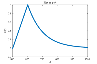
Figure 1: An illustration of a function in Class ${\mathcal{B}}$

Now we present our first convergence theorem, which is an extension of Lemma 1. Though the proof is straight-forward, we will see that it is a useful tool to establish the convergence of stochastic gradient methods for nonconvex functions.

Theorem 1.

Suppose $\{z_{t}\},\{f_{t}\},\{g_{t}\},\{h_{t}\},\{\alpha_{t}\}$ are $[0,\infty)$-valued stochastic processes defined on some probability space $(\Omega,\Sigma,P)$, and adapted to some filtration $\{{\mathcal{F}}_{t}\}$. Suppose further that

$$E_{t}(z_{t+1})\leq(1+f_{t})z_{t}+g_{t}-\alpha_{t}h_{t}\mbox{ a.s.},\;\forall t.$$ (14)

Define

$$\Omega_{0}:=\{\omega\in\Omega:\sum_{t=0}^{\infty}f_{t}(\omega)<\infty\mbox{ and }\sum_{t=0}^{\infty}g_{t}(\omega)<\infty\mbox{ and }\sum_{t=0}^{\infty}\alpha_{t}(\omega)=\infty\}.$$ (15)

Then

1. There exists a random variable $W$ defined on $(\Omega,\Sigma,P)$ such that $z_{t}(\omega)\rightarrow W(\omega)$ for all $\omega\in\Omega_{0}$. Moreover

   $$\liminf_{t\rightarrow\infty}h_{t}(\omega)=0\;\forall\omega\in\Omega_{0}.$$ (16)

2. Suppose there exists a function $\eta(\cdot)$ of Class ${\mathcal{B}}$ such that $h_{t}(\omega)\geq\eta(z_{t}(\omega))$ for all $\omega\in\Omega_{0}$. Then $z_{t}(\omega)\rightarrow 0$ as $t\rightarrow\infty$ for all $\omega\in\Omega_{0}$.

Proof.

By Lemma 1, there exist a random variable $W$ such that $z_{t}(\omega)\rightarrow W(\omega)$ as $t\rightarrow\infty$. Moreover,

$$\sum_{t=0}^{\infty}\alpha_{t}(\omega)h_{t}(\omega)<\infty,\;\forall\omega\in\Omega_{0}.$$

Now, by definition

$$\sum_{t=0}^{\infty}\alpha_{t}(\omega)=\infty,\;\forall\omega\in\Omega_{0}.$$

Therefore (16) follows. This is Item 1.

To prove item 2, suppose that, for some $\omega\in\Omega_{0}$, we have that $W(\omega)>0$, say $W(\omega)=:2\epsilon>0$. Choose a time $T$ such that $z_{t}(\omega)\geq\epsilon$ for all $t\geq T$. Also, by Item 1,

$$M:=\sup_{t\geq T}z_{t}(\omega)<\infty.$$

Next, since $\eta(\cdot)$ belongs to Class ${\mathcal{B}}$, it follows that

$$c:=\inf_{\epsilon\leq r\leq M}\eta(r)>0.$$

So, for $t\geq T$, we have that

$$h_{t}(\omega)\geq\eta(z_{t}(\omega))\geq c.$$

Now, if we discard all terms for $t<T$, we get

$$\sum_{t=T}^{\infty}\alpha_{t}(\omega)h_{t}(\omega)<\infty,\;\forall\omega\in\Omega_{0},\sum_{t=T}^{\infty}\alpha_{t}(\omega)=\infty,h_{t}(\omega)\geq c>0,$$

which is clearly a contradiction. Therefore the set of $\omega\in\Omega_{0}$ for which $W(\omega)>0$ has zero measure within $\Omega_{0}$. In other words, $z_{t}(\omega)\rightarrow 0$ for (almost) all $\omega\in\Omega_{0}$. This is Item 2. ∎

Theorem 1 above shows only that $z_{t}$ converges to $0$ almost surely on sample paths in $\Omega_{0}$. In this paper, we are interested not only in the convergence of various algorithms, but also on the rate of convergence. With this in mind, we now state and prove an extension of Theorem 1 that provides such an estimate on rates. For the purposes of this paper, we use the following definition inspired by [23].

Definition 2.

Suppose $\{Y_{t}\}$ is a stochastic process, and $\{f_{t}\}$ is a sequence of positive numbers. We say that

1. $Y_{t}=O(f_{t})$ if $\{Y_{t}/f_{t}\}$ is bounded almost surely.

2. $Y_{t}=\Omega(f_{t})$ if $Y_{t}$ is positive almost surely, and $\{f_{t}/Y_{t}\}$ is bounded almost surely.

3. $Y_{t}=\Theta(f_{t})$ if $Y_{t}$ is both $O(f_{t})$ and $\Omega(f_{t})$.

4. $Y_{t}=o(f_{t})$ if $Y_{t}/f_{t}\rightarrow 0$ almost surely as $t\rightarrow\infty$.

The next theorem is a modification of Theorem 1 that provides bounds on the rate of convergence. Hence forth, all assumptions hold “almost surely,” that is, along almost all sample paths. Hence we drop this modifier hereafter, it being implicitly understood.

Theorem 2.

Suppose $\{z_{t}\},\{f_{t}\},\{g_{t}\},\{\alpha_{t}\}$ are stochastic processes defined on some probability space $(\Omega,\Sigma,P)$, taking values in $[0,\infty)$, adapted to some filtration $\{{\mathcal{F}}_{t}\}$. Suppose further that

$$E_{t}(z_{t+1})\leq(1+f_{t})z_{t}+g_{t}-\alpha_{t}z_{t}\;\forall t,$$ (17)

where

$$\sum_{t=0}^{\infty}f_{t}(\omega)<\infty,\sum_{t=0}^{\infty}g_{t}(\omega)<\infty,\sum_{t=0}^{\infty}\alpha_{t}(\omega)=\infty.$$

Then $z_{t}=o(t^{-\lambda})$ for every $\lambda\in(0,1]$ such that (i) there exists a $T<\infty$ such that

$$\alpha_{t}(\omega)-\lambda t^{-1}\geq 0\;\forall t\geq T,$$ (18)

and in addition (ii)

$$\sum_{t=0}^{\infty}(t+1)^{\lambda}g_{t}(\omega)<\infty,\sum_{t=0}^{\infty}[\alpha_{t}(\omega)-\lambda t^{-1}]=\infty.$$ (19)

Proof.

Since the map $t\mapsto t^{\lambda}$ is concave for $\lambda\in(0,1)$, it follows from the “graph below the tangent” property that

$$(t+1)^{\lambda}\leq t^{\lambda}+\lambda t^{\lambda-1}.$$ (20)

This is the same as [23, Eq. (25)] with the substitution $\lambda=1-\epsilon$. Now a ready consequence of (20) is

$$1\leq\left(\frac{t+1}{t}\right)^{\lambda}\leq 1+\lambda t^{-1}.$$

Now we follow the suggestion of [23, Lemma 1] by recasting (18) in terms of $t^{\lambda}z_{t}$. If we multiply both sides of (18) by $(t+1)^{\lambda}$, and divide by $t^{\lambda}$ where appropriate, we get

$$E_{t}((t+1)^{\lambda}z_{t+1})\leq(1+f_{t})\left(\frac{t+1}{t}\right)^{\lambda}t^{\lambda}z_{t}+(t+1)^{\lambda}g_{t}-\alpha_{t}\left(\frac{t+1}{t}\right)^{\lambda}t^{\lambda}z_{t}.$$

Now we observe that

$$-\alpha_{t}\left(\frac{t+1}{t}\right)^{\lambda}\leq-\alpha_{t},$$

$$(1+f_{t})\left(\frac{t+1}{t}\right)^{\lambda}\leq(1+f_{t})(1+\lambda t^{-1})=1+f_{t}(1+\lambda t^{-1})+\lambda t^{-1}.$$

If we now define the modified quantity $\bar{z}_{t}=t^{\lambda}z_{t}$, then the above bound can be rewritten as

$$E_{t}(\bar{z}_{t+1})\leq[1+f_{t}(1+\lambda t^{-1})]\bar{z}_{t}+(t+1)^{\lambda}g_{t}-(\alpha_{t}-\lambda t^{-1})\bar{z}_{t}.$$ (21)

It is obvious that

$$\sum_{t=0}^{\infty}f_{t}<\infty\;\Longrightarrow\;\sum_{t=0}^{\infty}f_{t}(1+\lambda t^{-1})<\infty.$$

Moreover, by assumption, there exists a finite $T$ such that

$$\alpha_{t}-\lambda t^{-1}\geq 0,\;\forall t\geq T.$$

Since it is always permissible to analyze the inequality (18) starting at time $T$, we can apply Theorem 1 to (18), with $\eta(r)=r$, and deduce that $\bar{z}_{t}\rightarrow 0$ as $t\rightarrow\infty$. This is equivalent to $z_{t}=o(t^{-\lambda})$. ∎

2.2 Applications of the Convergence Theorems with Rates

In this subsection, we apply the Theorems 1 and 2 to a specific problem that occurs repeatedly in nonconvex optimization, Reinforcement Learning etc. Recall the notation introduced earlier: For any ${\mathbb{R}}^{d}$-valued random variable $X$ and a $\sigma$-algebra ${\mathcal{F}}_{t}$, denote $E(X|{\mathcal{F}}_{t})$ by $E_{t}(X)$ (as before), and define its conditional variance via

$$CV_{t}(X)=E_{t}(\|X-E_{t}(X)\|_{2}^{2}).$$

Now for the problem under study. Suppose ${\boldsymbol{\theta}}_{0}$ is an ${\mathbb{R}}^{d}$-valued random variable, and that $\{{\boldsymbol{\zeta}}_{t}\}_{t\geq 1}$ is an ${\mathbb{R}}^{d}$-valued stochastic process. Define $\{{\boldsymbol{\theta}}_{t},t\geq 1\}$ by

$${\boldsymbol{\theta}}_{t+1}=(1-\alpha_{t}){\boldsymbol{\theta}}_{t}+\alpha_{t}{\boldsymbol{\zeta}}_{t+1},t\geq 0,$$ (22)

where $\{\alpha_{t}\}_{t\geq 0}$ is another $[0,1)$-valued stochastic process. Define $\{{\mathcal{F}}_{t}\}$ to be the filtration where ${\mathcal{F}}_{t}$ is the $\sigma$-algebra generated by ${\boldsymbol{\theta}}_{0},\alpha_{0}^{t},{\boldsymbol{\zeta}}_{1}^{t}$. For convenience, define

$${\boldsymbol{\eta}}_{t}=E_{t}({\boldsymbol{\zeta}}_{t+1}),{\boldsymbol{\psi}}_{t+1}={\boldsymbol{\zeta}}_{t+1}-{\boldsymbol{\eta}}_{t},$$

and observe that $E_{t}({\boldsymbol{\psi}}_{t+1})={\bf 0}$.

With these conventions, we first state a result on convergence, but without any estimate of the rate of convergence. Note that (22) is of the form (2) with ${\bf g}({\boldsymbol{\theta}})\equiv{\bf 0}$. Hence ${\bf g}(\cdot)$ has the unique fixed point ${\bf 0}$, and we would want that ${\boldsymbol{\theta}}_{t}\rightarrow{\bf 0}$ as $t\rightarrow\infty$.

Theorem 3.

Suppose there exist sequences of constants $\{\mu_{t}\}$, $\{M_{t}\}$ such that, for all $t\geq 0$ we have

$$\|E_{t}({\boldsymbol{\zeta}}_{t+1})\|_{2}=\|{\boldsymbol{\eta}}_{t}\|_{2}\leq\mu_{t}(1+\|{\boldsymbol{\theta}}_{t}\|_{2}),$$ (23)

$$CV_{t}({\boldsymbol{\zeta}}_{t+1})=E_{t}(\|{\boldsymbol{\psi}}_{t+1}\|_{2}^{2})\leq M_{t}^{2}(1+\|{\boldsymbol{\theta}}_{t}\|_{2}^{2}).$$ (24)

Under these conditions, if

$$\sum_{t=0}^{\infty}\alpha_{t}^{2}<\infty,\sum_{t=0}^{\infty}\mu_{t}\alpha_{t}<\infty,\sum_{t=0}^{\infty}M^{2}_{t}\alpha^{2}_{t}<\infty,$$ (25)

then $\{{\boldsymbol{\theta}}_{t}\}$ is bounded, and $\|{\boldsymbol{\theta}}_{t}\|_{2}$ converges to an ${\mathbb{R}}^{d}$-valued random variable. If in addition,

$$\sum_{t=0}^{\infty}\alpha_{t}=\infty,$$ (26)

then ${\boldsymbol{\theta}}_{t}\rightarrow{\bf 0}$.

Proof.

(Of Theorem 3:) The proof consists of finding an upper bound for $E_{t}(\|{\boldsymbol{\theta}}_{t+1}\|_{2}^{2})$ and then applying Theorem 1. Throughout, we use the simple identity $2x\leq 1+x^{2}$ for all $x\in{\mathbb{R}}$. We begin by noting that

$$\|{\boldsymbol{\theta}}_{t+1}\|_{2}^{2} = \langle{\boldsymbol{\theta}}_{t+1},{\boldsymbol{\theta}}_{t+1}\rangle$$

$$= (1-\alpha_{t})^{2}\|{\boldsymbol{\theta}}_{t}\|_{2}^{2}+2\alpha_{t}(1-\alpha_{t})\langle{\boldsymbol{\theta}}_{t},{\boldsymbol{\zeta}}_{t+1}\rangle+\alpha_{t}^{2}\|{\boldsymbol{\zeta}}_{t+1}\|_{2}^{2}.$$

First, observe that

$$(1-\alpha_{t})^{2}\|{\boldsymbol{\theta}}_{t}\|_{2}^{2}=\|{\boldsymbol{\theta}}_{t}\|_{2}^{2}+\alpha_{t}^{2}\|{\boldsymbol{\theta}}_{t}\|_{2}^{2}-2\alpha_{t}\|{\boldsymbol{\theta}}_{t}\|_{2}^{2}.$$

Next, let us bound the conditional expectations of the last two terms. This gives

$$E_{t}(\langle{\boldsymbol{\theta}}_{t},{\boldsymbol{\zeta}}_{t+1}\rangle)=\langle{\boldsymbol{\theta}}_{t},{\boldsymbol{\eta}}_{t}\rangle,$$

because $E_{t}(\langle{\boldsymbol{\theta}}_{t},{\boldsymbol{\psi}}_{t+1}\rangle)=0$. Hence

$$|E_{t}(\langle{\boldsymbol{\theta}}_{t},{\boldsymbol{\zeta}}_{t+1}\rangle)|\leq\|{\boldsymbol{\eta}}_{t}\|_{2}\|{\boldsymbol{\theta}}_{t}\|_{2}\leq\mu_{t}(\|{\boldsymbol{\theta}}_{t}\|_{2}+\|{\boldsymbol{\theta}}_{t}\|_{2}^{2})\leq\mu_{t}(0.5+1.5\|{\boldsymbol{\theta}}_{t}\|_{2}^{2}).$$

Now note that $1-\alpha_{t}\leq 1$. Therefore

$$2\alpha_{t}(1-\alpha_{t})E_{t}(\langle{\boldsymbol{\theta}}_{t},{\boldsymbol{\zeta}}_{t+1}\rangle)\leq\alpha_{t}\mu_{t}(1+3\|{\boldsymbol{\theta}}_{t}\|_{2}^{2}).$$

Next,

$$E_{t}(\|{\boldsymbol{\zeta}}_{t+1}\|_{2}^{2}) = \|{\boldsymbol{\eta}}_{t}\|_{2}^{2}+E_{t}(\|{\boldsymbol{\psi}}_{t+1}\|_{2}^{2})\leq\mu_{t}^{2}(1+\|{\boldsymbol{\theta}}_{t}\|_{2})^{2}+M_{t}^{2}(1+\|{\boldsymbol{\theta}}_{t}\|_{2}^{2})$$

$$\leq (2\mu_{t}^{2}+M_{t}^{2})(1+\|{\boldsymbol{\theta}}_{t}\|_{2}^{2}).$$

Combining everything gives

$$E_{t}(\|{\boldsymbol{\theta}}_{t+1}\|_{2}^{2}) \leq \|{\boldsymbol{\theta}}_{t}\|_{2}^{2}+[\alpha_{t}^{2}(1+2\mu_{t}^{2}+M_{t}^{2})+3\alpha_{t}\mu_{t}]\|{\boldsymbol{\theta}}_{t}\|_{2}^{2}$$

$$+ \alpha_{t}^{2}(2\mu_{t}^{2}+M_{t}^{2})+\alpha_{t}\mu_{t}-2\alpha_{t}\|{\boldsymbol{\theta}}_{t}\|_{2}^{2}$$

Now apply Theorem 1 with

$$z_{t}=\|{\boldsymbol{\theta}}_{t}\|_{2}^{2},f_{t}=\alpha_{t}^{2}(1+2\mu_{t}^{2}+M_{t}^{2})+3\alpha_{t}\mu_{t},g_{t}=\alpha_{t}^{2}(2\mu_{t}^{2}+M_{t}^{2})+\alpha_{t}\mu_{t}.$$

If (25) holds, then

$$\sum_{t=0}^{\infty}\alpha_{t}\mu_{t}<\infty\;\Longrightarrow\;\sum_{t=0}^{\infty}\alpha_{t}^{2}\mu_{t}^{2}<\infty.$$

Therefore the sequences $\{f_{t}\}$ and $\{g_{t}\}$ are summable. It follows from Item 1 of Theorem 1 that $\{\|{\boldsymbol{\theta}}_{t}\|_{2}^{2}\}$ is bounded, and converges to some random variable $W$. Next, suppose (26) also holds. We apply Item 2 of Theorem 1 with $\eta(z_{t})=2z_{t}$, which is clearly a function of Class ${\mathcal{B}}$. Therefore $z_{t}=\|{\boldsymbol{\theta}}_{t}\|_{2}^{2}\rightarrow 0$, and ${\boldsymbol{\theta}}_{t}\rightarrow{\bf 0}$. ∎

Theorem 3 above shows only that the vector ${\boldsymbol{\theta}}_{t}$ converges to ${\bf 0}$ almost surely. Now we combine this theorem with Theorem 2 to obtain bounds on the rate of convergence.

The following pair of conditions, commonly referred to as the Robbins-Monro or RM conditions, were first introduced in [34]. Note that in these conditions, $\{\alpha_{t}\}$ is a sequence of real numbers, not random variables.

$$\sum_{t=0}^{\infty}\alpha_{t}^{2}<\infty,\sum_{t=0}^{\infty}\alpha_{t}=\infty.$$ (28)

However, in this paper, $\{\alpha_{t}\}$ can be random, and (28) is permitted to hold almost surely. These requirements provide a considerable amount of latitude in how to choose $\alpha_{t}$. A common choice is

$$\alpha_{t}=\frac{C}{(t+1)^{1-\phi}}=C(t+1)^{-(1-\phi)},$$ (29)

where any $\phi\in(0,0.5)$ satisfies RM conditions. With this motivation, we present a refinement of Theorem 3.

Theorem 4.

Let various symbols be as in Theorem 3. Further, suppose there exist constants $\gamma>0$ and $\delta\geq 0$ such that

$$\mu_{t}=O(t^{-\gamma}),M_{t}=O(t^{\delta}),$$

where we take $\gamma=1$ if $\mu_{t}=0$ for all sufficiently large $t$, and $\delta=0$ if $M_{t}$ is bounded. Choose the step-size sequence $\{\alpha_{t}\}$ as $O(t^{-(1-\phi)})$ and $\Omega(t^{-(1-c)})$ where $\phi$ is chosen to satisfy

$$0<\phi<\min\{0.5-\delta,\gamma\},$$

and $c\in(0,\phi]$. Define

$$\nu:=\min\{1-2(\phi+\delta),\gamma-\phi\}.$$ (30)

Then $\|{\boldsymbol{\theta}}_{t}\|_{2}^{2}=o(t^{-\lambda})$ for every $\lambda\in(0,\nu)$. In particular, if $\mu_{t}=0$ for all $t$ and $M_{t}$ is bounded with respect to $t$, then we can take $\nu=1-2\phi$.

Proof.

Define $V_{t}=\|{\boldsymbol{\theta}}_{t}\|_{2}^{2}$. We already know from (LABEL:eq:2110) that

$$E_{t}(V_{t+1})\leq(1+f_{t})V_{t}+g_{t}-2\alpha_{t}V_{t},$$ (31)

where

$$f_{t}=\alpha_{t}^{2}(1+2\mu_{t}^{2}+M_{t}^{2})+3\alpha_{t}\mu_{t},g_{t}=\alpha_{t}^{2}(2\mu_{t}^{2}+M_{t}^{2})+\alpha_{t}\mu_{t}.$$

Under the stated hypotheses, it readily follows that

$$\alpha_{t}^{2}=O(t^{-2+2\phi}),\alpha_{t}^{2}M_{t}^{2}=O(t^{-2+2(\phi+\delta)}),\alpha_{t}\mu_{t}=O(t^{-1+\phi-\gamma}).$$

Since $\delta\geq 0$, it follows that $f_{t}=O(t^{-(1+\nu)})$, where $\nu$ is defined as in (30). Similarly, after noting that $\{\alpha_{t}^{2}\mu_{t}^{2}\}$ decays faster than $\{\alpha_{t}\mu_{t}\}$, we deduce that $g_{t}=O(t^{-1+\phi-\gamma})$. Hence, with $\nu$ defined as in (31),

$$f_{t},g_{t}=O(t^{-(1+\nu)}),$$

and both sequences are summable.

Now we are in a position to apply Theorem 2. We can conclude that $V_{t}=o(t^{-\lambda})$ whenever $2\alpha_{t}-\lambda t^{-1}\geq 0$ for sufficiently large $t$, and

$$\{(t+1)^{\lambda}g_{t}\}\in\ell_{1},$$ (32)

$$\sum_{t=0}^{\infty}[2\alpha_{t}-\lambda t^{-1}]=\infty.$$ (33)

Now observe that $2\alpha_{t}=\Omega(t^{-(1-c)})$, and $c>0$. Hence $2\alpha_{t}-\lambda t^{-1}\geq 0$ for sufficiently large $t$, and

$$\sum_{t=0}^{\infty}(2\alpha_{t}-\lambda t^{-1})=\infty,$$ (34)

which is (33). Thus the last step of the proof is to determine conditions under which $\{(t+1)^{\lambda}g_{t}\}\in\ell_{1}$. Since $g_{t}=O(t^{-(1+\nu)})$, it follows that $(t+1)^{\lambda}g_{t}=O(t^{-(1+\nu-\lambda)})$, which is summable if $\lambda<\nu$. Hence, whenever $\lambda<\nu$, we conclude that $\bar{V}_{t}\rightarrow 0$ almost surely, or equivalently, that $V_{t}=o(t^{-\lambda})$. This completes the proof. ∎

3 Convergence of Stochastic Gradient Descent

In this section, we apply the results proved in Section 2 to analyze the convergence of various methods for minimizing a class of nonconvex functions; this class includes convex functions as a subset. We analyze the so-called Stochastic Gradient Descent (SGD) method, wherein the search direction is a noise-corrupted measurement of the current gradient. We estimate the rate of convergence of the algorithm. Specifically, we show that the “optimal” step size sequence is $\alpha_{t}=O(t^{-(1-\phi)})$, where $\phi$ is arbitrarily small. In turn this leads to the SGD converging at the rate of $o(t^{-\lambda})$, where $\lambda$ is arbitrarily close to one. Since the fastest known rate of convergence of SGD even with noise-free measurements is $O(t^{-1})$, this shows that the fastest rate of convergence can be preserved despite the presence of measurement errors.

The reader is cautioned that some authors use the phrase “stochastic gradient” to refer to the situation where only one randomly selected component of ${\boldsymbol{\theta}}_{t}$ is updated at each time $t$. In this usage of the phrase SGD, it is common to assume that the measurements of the gradient are not corrupted by any noise. This assumption facilitates a very detailed analysis of the algorithms. Good surveys of such methods are found in [46, 42]. However, such analyses are no longer applicable when the gradient measurements are corrupted by mesurement errors.

3.1 Assumptions

We begin by stating various assumptions on the function $J(\cdot)$ that we seek to minimize. Note that it is not assumed that $J(\cdot)$ is convex. First there are a couple of standard assumptions:

1. The function $J(\cdot)$ is bounded below and has a unique global minimum. By translating coordinates, it is assumed that the global minimum value of $J(\cdot)$ is zero, and occurs at ${\boldsymbol{\theta}}^{*}={\bf 0}$.

2. The function $J(\cdot)$ has compact level sets; thus, for each constant $c$, the set

   $$L_{J}(c):=\{{\boldsymbol{\theta}}:J({\boldsymbol{\theta}})\leq c\}$$

   is compact. Note that some authors use the adjective “coercive” to refer to such functions.

These assumptions are made in every theorem, and thus not repeated every time.

The above assumptions are fairly standard. Now we state the “operative” assumptions. Note that different subsets of assumptions are used in different theorems.

1. $J:{\mathbb{R}}^{d}\rightarrow{\mathbb{R}}$ is ${\mathcal{C}}^{1}$, and $\nabla J(\cdot)$ is Lipschitz-continuous with constant $L$.

2. There exists a constant $H$ such that

   $$\|\nabla J({\boldsymbol{\theta}})\|_{2}^{2}\leq HJ({\boldsymbol{\theta}}),\;\forall{\boldsymbol{\theta}}\in{\mathbb{R}}^{d}.$$ (35)

3. There exists a function $\psi(\cdot)$ of Class ${\mathcal{B}}$ such that

   $$\|\nabla J({\boldsymbol{\theta}})\|_{2}^{2}\geq\psi(J({\boldsymbol{\theta}})),\;\forall{\boldsymbol{\theta}}\in{\mathbb{R}}^{d}.$$ (36)

4. There exists a constant $K$ such that

   $$\|\nabla J({\boldsymbol{\theta}})\|_{2}^{2}\geq KJ({\boldsymbol{\theta}}),\;\forall{\boldsymbol{\theta}}\in{\mathbb{R}}^{d}.$$ (37)

Now we discuss the significance of these assumptions. Assumption (J1) guarantees that $J({\boldsymbol{\theta}})=O(\|{\boldsymbol{\theta}}\|_{2}^{2})$. If $J(\cdot)$ is convex, then it is known that Assumption (J2) is satisfied with $H=2L$; see [27, Theorem 2.1.5]. If in addition $J(\cdot)$ is also $R$-strongly convex, in the sense that

$$J({\boldsymbol{\psi}})\geq J({\boldsymbol{\theta}})+\langle\nabla J({\boldsymbol{\theta}}),{\boldsymbol{\psi}}-{\boldsymbol{\theta}}\rangle+\frac{R}{2}\|{\boldsymbol{\psi}}-{\boldsymbol{\theta}}\|_{2}^{2},$$

for some constant $R$, then it follows from [27, Theorem 2.1.10] that

$$J({\boldsymbol{\theta}})\leq\frac{1}{2R}\|\nabla J({\boldsymbol{\theta}}\|_{2}^{2},\;\forall{\boldsymbol{\theta}}\in{\mathbb{R}}^{d}.$$

Thus $J(\cdot)$ satisfies Assumption (J3’) with $K=1/2R$. Note that Assumption (J3) is weaker than Assumption (J3’). To ilustrate this, consider the map $J:{\mathbb{R}}\rightarrow{\mathbb{R}}$ defined by $J(\theta)=|\theta|^{p}$, where $p\in(1,2)$. Also, there exist nonconvex functions that also satisfy these assumptions. See Examples 2 and 3 below.

3.2 Convergence Theorems

The general class of algorithms studied in this section and the next is now described. Begin with an initial guess ${\boldsymbol{\theta}}_{0}\in{\mathbb{R}}^{d}$ which could be random. At each time $t+1\geq 1$, choose a search direction ${\bf h}_{t+1}$ which is random; different algorithms differ in the manner in which the search direction is chosen. Choose a step size $\alpha_{t}$, which could also be random. Then update the guess via

$${\boldsymbol{\theta}}_{t+1}={\boldsymbol{\theta}}_{t}-\alpha_{t}{\bf h}_{t+1}.$$ (38)

In the case of the SGD (Stochastic Gradient Descent) algorithm studied in this section, we choose

$${\bf h}_{t+1}=\nabla J({\boldsymbol{\theta}}_{t})+{\boldsymbol{\xi}}_{t+1},$$ (39)

where ${\boldsymbol{\xi}}_{t+1}$ is a measurement error. In the next section, more general choices for ${\bf h}_{t+1}$ are permitted. The mismatch in subscripts between $\alpha_{t}$ and ${\bf h}_{t+1}$ is intended to suggest the following. Let $\{{\mathcal{F}}_{t}\}$ denote a filtration with respect to which ${\boldsymbol{\theta}}_{0},\alpha_{0}^{t},{\bf h}_{1}^{t}$ are measurable. Thus the step size $\alpha_{t}$ at time $t+1$ is chosen, possibly in a random manner, based on the information available at up to time $t$. However, the search direction ${\bf h}_{t+1}$ at time $t+1$ need not be measurable with respect to ${\mathcal{F}}_{t}$.

Define

$${\bf z}_{t}:=E_{t}({\bf h}_{t+1}),{\boldsymbol{\zeta}}_{t+1}:={\bf h}_{t+1}-{\bf z}_{t},$$ (40)

This definition ensures that

$$E_{t}({\boldsymbol{\zeta}}_{t+1})={\bf 0},CV_{t}({\bf h}_{t+1})=E_{t}(\|{\boldsymbol{\zeta}}_{t+1}\|_{2}^{2}).$$ (41)

If the direction ${\bf h}_{t+1}$ is chosen as in (39), then

$$CV_{t}({\bf h}_{t+1})=E_{t}(\|{\boldsymbol{\xi}}_{t+1}\|_{2}^{2}.$$

This implies that the quantities defined in (40) are given by

$${\bf z}_{t}=\nabla J({\boldsymbol{\theta}}_{t}),{\boldsymbol{\zeta}}_{t+1}={\boldsymbol{\xi}}_{t+1}.$$

Thus (39) represents full-coordinate gradient descent using noise-corrupted gradients. The following are the assumptions on the measurement error.

1. We have that

   $$E_{t}({\boldsymbol{\xi}}_{t+1})={\bf 0},\;\forall t\geq 0.$$ (42)

   This implies that ${\bf h}_{t+1}$ in (39) is an unbiased measurement of $\nabla J({\boldsymbol{\theta}}_{t})$.

2. There exists a constant $M$ such that

   $$CV_{t}({\boldsymbol{\xi}}_{t+1})\leq M^{2}(1+\|\nabla J({\boldsymbol{\theta}}_{t})\|_{2}^{2}),\;\forall t\geq 0.$$ (43)

   Note that if (J2) holds, then

   $$CV_{t}({\boldsymbol{\xi}}_{t+1})\leq M^{2}(1+HJ({\boldsymbol{\theta}}_{t})).$$ (44)

With this background, we state the first convergence result, which does not have any conclusions about the rate of convergence. Subsequently, we replace Assumption (J3) by (J3’), and also derive bounds on the rate of convergence. Since the various conclusions hold almost surely, we omit this phrase, to avoid tedious repetition.

Theorem 5.

Suppose the objective function $J(\cdot)$ satisfies Assumptions (J1) and (J2), and that the error term ${\boldsymbol{\xi}}_{t+1}$ satisfies Assumptions (N1) and (N2). Under these conditions, we have the following conclusions:

1. If

   $$\sum_{t=0}^{\infty}\alpha_{t}^{2}<\infty,$$ (45)

   then $\{\nabla J({\boldsymbol{\theta}}_{t})\}$ and $\{J({\boldsymbol{\theta}}_{t})\}$ are bounded.

2. If in addition $J(\cdot)$ also satisfies Assumption (J3), and

   $$\sum_{t=0}^{\infty}\alpha_{t}=\infty,$$ (46)

   then $J({\boldsymbol{\theta}})\rightarrow 0$ and $\nabla J({\boldsymbol{\theta}}_{t})\rightarrow{\bf 0}$ as $t\rightarrow\infty$.

Proof.

We first prove Item 1. Observe that

$$J({\boldsymbol{\theta}}_{t+1})=J({\boldsymbol{\theta}}-\alpha_{t}{\bf h}_{t+1}).$$

Hence it follows from [3, Eq. (2.4)] that

$$J({\boldsymbol{\theta}}_{t+1})\leq J({\boldsymbol{\theta}}_{t})-\alpha_{t}\langle\nabla J({\boldsymbol{\theta}}_{t}),{\bf h}_{t+1}\rangle+\frac{\alpha_{t}^{2}L}{2}\|{\bf h}_{t+1}\|_{2}^{2}.$$

The next step is to apply the $E_{t}$ operation to both sides. This is facilitated by two observations, both using $E_{t}({\boldsymbol{\xi}}_{t+1})={\bf 0}$. First,

$$E_{t}(\langle\nabla J({\boldsymbol{\theta}}_{t}),{\bf h}_{t+1}\rangle)=\langle\nabla J({\boldsymbol{\theta}}_{t}),E_{t}({\bf h}_{t+1})\rangle=\|\nabla J({\boldsymbol{\theta}}_{t})\|_{2}^{2}.$$

Second,

$$E_{t}(\|{\bf h}_{t+1}\|_{2}^{2}) = \|\nabla J({\boldsymbol{\theta}}_{t})\|_{2}^{2}+CV_{t}({\boldsymbol{\xi}}_{t+1})\leq\|\nabla J({\boldsymbol{\theta}}_{t})\|_{2}^{2}+M^{2}(1+\|\nabla J({\boldsymbol{\theta}}_{t})\|_{2}^{2})$$

$$\leq HJ({\boldsymbol{\theta}}_{t})+M^{2}(1+HJ({\boldsymbol{\theta}}_{t}))=M^{2}+H(1+M^{2})J({\boldsymbol{\theta}}_{t}).$$

Combining everything leads to

$$E_{t}(J({\boldsymbol{\theta}}_{t+1})) \leq J({\boldsymbol{\theta}}_{t})+\frac{\alpha_{t}^{2}L}{2}[\|\nabla J({\boldsymbol{\theta}}_{t})\|_{2}^{2}+M^{2}(1+\|\nabla J({\boldsymbol{\theta}}_{t})\|_{2}^{2})]$$

$$- \alpha_{t}\|\nabla J({\boldsymbol{\theta}}_{t})\|_{2}^{2}.$$

Now, if we invoke Assumption (J2) and rearrange terms, we get

$$E_{t}(J({\boldsymbol{\theta}}_{t+1})) \leq J({\boldsymbol{\theta}}_{t})+\alpha_{t}^{2}\frac{LH(1+M^{2})}{2}J({\boldsymbol{\theta}}_{t})+\frac{\alpha_{t}^{2}LM^{2}}{2}$$ (47)

$$- \alpha_{t}\|\nabla J({\boldsymbol{\theta}}_{t})\|_{2}^{2}.$$

Now, if (45) holds, then we can apply Theorem 1 with

$$z_{t}=J({\boldsymbol{\theta}}),f_{t}=\alpha_{t}^{2}\frac{LH(1+M^{2})}{2},g_{t}=\frac{\alpha_{t}^{2}LM^{2}}{2},h_{t}=\|\nabla J({\boldsymbol{\theta}}_{t})\|_{2}^{2}.$$

Note that both $f_{t}$ and $g_{t}$ are real-valued sequences and not random. Moreover, both sequences are summable. Thus Theorem 1 leads to the conclusion that $\{J({\boldsymbol{\theta}}_{t})\}$ is bounded. Now Assumption (J2) implies that $\{\nabla J({\boldsymbol{\theta}}_{t})\}$ is also bounded.

Next we prove Item 2. Suppose (46) holds. Then we apply Theorem 1, and conclude that

$$\sum_{t=0}^{\infty}\alpha_{t}\|\nabla J({\boldsymbol{\theta}}_{t})\|_{2}^{2}<\infty.$$

Now suppose (J3) holds, so that $\|\nabla J({\boldsymbol{\theta}}_{t})\|_{2}^{2}\geq\psi(J({\boldsymbol{\theta}}_{t}))$ for some Class ${\mathcal{B}}$ function $\psi(\cdot)$. Then it again follows from Theorem 1 that $j({\boldsymbol{\theta}}_{t})\rightarrow 0$ as $t\rightarrow\infty$. Finally, applying Assumption (J2) shows that $\nabla J({\boldsymbol{\theta}}_{t})\rightarrow{\bf 0}$. ∎

Next we strengthen Assumption (J3) to (J3’), and prove an estimate for the rate of convergence.

Theorem 6.

Suppose that, in Theorem 5, Item 2, Assumption (J3) is replaced by Assumption (J3’), and that the step size sequence satisfies

$$\alpha_{t}=O(t^{-(1-\phi)}),\alpha_{t}=\Omega(t^{-(1-c)}),c\in(0,\phi]$$

for some $\phi\in(0,0.5)$. Then $J({\boldsymbol{\theta}}_{t}),\|\nabla J({\boldsymbol{\theta}}_{t})\|_{2}^{2}=o(t^{-\lambda})$ for every $\lambda<1-2\phi$.

Proof.

Suppose Assumption (J3’) holds. Then (47) can be rewritten as

$$E_{t}(J({\boldsymbol{\theta}}_{t+1})) \leq J({\boldsymbol{\theta}}_{t})+\frac{\alpha_{t}^{2}L}{2}[\|\nabla J({\boldsymbol{\theta}}_{t})\|_{2}^{2}+M^{2}(1+\|\nabla J({\boldsymbol{\theta}}_{t})\|_{2}^{2})]$$ (48)

$$- \alpha_{t}KJ({\boldsymbol{\theta}}_{t})$$

$$= (1+\alpha_{t}^{2}C_{1}J({\boldsymbol{\theta}}_{t})+\alpha_{t}^{2}C_{2}-\alpha_{t}KJ({\boldsymbol{\theta}}_{t})$$

for suitable constants $C_{1},C_{2}$. Now we can apply Theorem 2 with

$$f_{t}=\alpha_{t}^{2}C_{1},g_{t}=\alpha_{t}^{2}C_{2}.$$

Hence $J({\boldsymbol{\theta}}_{t})=o(t^{-\lambda})$ whenever $\{\alpha_{t}^{2}(t+1)^{\lambda}\}\in\ell_{1}$, $K\alpha_{t}-\lambda t^{-1}\geq 0$ for sufficiently large $t$, and and

$$\sum_{t=0}^{\infty}(K\alpha_{t}-\lambda t^{-1})=\infty.$$

Now $\alpha_{t}^{2}(t+1)^{\lambda}=O(t^{-2(1-\phi)+\lambda})$, and the exponent of $t$ is $<-1$ if $2\phi+\lambda<1$, or $\lambda<1-2\phi$. Hence $\{\alpha_{t}^{2}(t+1)^{\lambda}\}\in\ell_{1}$ if $\lambda<1-2\phi$. Moreover, since $\alpha_{t}=\Omega(t^{-(1-c)})$ and $c>0$, it follows that $K\alpha_{t}-\lambda t^{-1}\geq 0$ for sufficiently large $t$. Finally, the divergence condition is satisfied whenever $\lambda\in(0,1]$. Therefore $J({\boldsymbol{\theta}}_{t})=o(t^{-\lambda})$ for all $\lambda\in(0,1-2\phi)$. ∎

Next we discuss an “optimal” choice for $\phi$. Clearly, the smaller $\phi$ is, the closer $\lambda$ is to $1$. Hence, if we choose $\phi=\epsilon$, a very small number, then $J({\boldsymbol{\theta}}_{t}),\|\nabla J({\boldsymbol{\theta}}_{t})\|_{2}^{2}=o(t^{-\lambda})$ for $\lambda$ arbitrarily close to $1-2\epsilon$. The conclusion is that the bound is optimized with very very small values of $\phi$, or step sizes decreasing just slightly faster than $(t+1)^{-1}$. With such a choice, $J({\boldsymbol{\theta}}_{t})=o(t^{-\lambda})$ for $\lambda$ arbitrarily close to $1$. Recall that $O(t^{-1})$ is the rate of convergence for the steepest descent method with a strongly convex objective function; see [28, Corollary 2.1.2] and [28, Eq. (2.1.39)]. Thus an important consequence of Theorem 6 is that, even with noisy measurements of the gradient, SGD can be made to converge at a rate arbitrarily close to the best achievable rate with noise-free measurements.

3.3 Examples

In this subsection, we present two examples of nonconvex functions that satisfy Assumptions (J3) or (J3’). In the first case, the objective function satisfies Assumptions (J1), (J2) and (J3), and the SGD algorithm converges, as shown in Theorem 5. In the second, the objective function satisfies Assumption (J3’) instead of (J3), which enables us to show that SGD can be made to converge at the rate of $o(t^{-(1-\epsilon)})$ for $\epsilon$ arbitrarily close to $0$, as shown in Theorem 6.

Example 2.

Let us return to the function $\phi(\cdot):{\mathbb{R}}_{+}\rightarrow{\mathbb{R}}_{+}$ defined in Example 1. Define $f:{\mathbb{R}}\rightarrow{\mathbb{R}}$ as the odd extension of $\phi$ and $J:{\mathbb{R}}\rightarrow{\mathbb{R}}$ as

$$J(\theta)=\int_{0}^{\theta}f(\theta)\;d\theta,$$

so that $f(\cdot)$ is the derivative of $J(\cdot)$. Figure 2 shows the function $J(\cdot)$ and its derivative $f(\cdot)$.

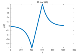
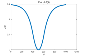
The function $f(\cdot)$	The function $J(\cdot)$

Figure 2: A nonconvex function

It is obvious that $J(\cdot)$ is not convex. Moreover, $f(\theta)\rightarrow 0$ as $|\theta|\rightarrow\infty$. Hence $J(\cdot)$ satisfies Assumptions (J1), (J2) and (J3), but not (J3’). Hence SGD converges in this case as a consequence of Theorem 5, but Theorem 6 does not apply.

Example 3.

In this example, we modify the function in Example 1 as follows: Define $\psi(0)=0$. If $n$ is an even integer (including zero), then

$$\psi(n+t)=\psi(n)+t,t\in[0,1].$$

If $n$ is an odd integer, then

$$\psi(n+t)=\psi(n)-\exp(t),t\in[0,1].$$

Then $\psi(\theta)$ is bounded above and below by linear functions of $\theta$. Hence, if we define $f$ to be the odd extension of $\psi$, and $J$ to be the function with $J(0)=0$ with derivative $f$, then $J$ is not convex. However, it does satisfy Assumptions (J1) , (J2) and (J3’). Hence, by choosing a step-size sequence $\alpha_{t}=O(t^{-(1-\epsilon)})$ $\alpha_{t}=O(t^{-(1-C)})$ where $0<C\leq\epsilon$, we can achieve a convergence rate for the SGD with rate arbitrarily close to $O(t^{-(1-\epsilon)})$.

4 Convergence of SGD with Approximate Gradients

In this section, we analyze the convergence of the SGD method when the exact gradient is replaced by a first-order approximation. Such an approach is referred to by a variety of names, such as gradient-free, zeroth order, etc. This idea was first suggested in [19] for the one-dimensional case, and extended to the case of higher dimensions in [5]. Indeed, the convergence conditions derived in these references, stated here as (10), are as standard as the Robbins-Monro conditions, though perhaps less well-known.

Recall the general form of the optimization algorithm:

$${\boldsymbol{\theta}}_{t+1}={\boldsymbol{\theta}}_{t}-\alpha_{t}{\bf h}_{t+1}.$$ (49)

Now define

$${\bf z}_{t}=E_{t}({\bf h}_{t+1}),{\boldsymbol{\zeta}}_{t+1}={\bf h}_{t+1}-{\bf z}_{t},{\bf x}_{t}={\bf z}_{t}-\nabla J({\boldsymbol{\theta}}_{t}).$$ (50)

In the previous section, we had ${\bf z}_{t}=\nabla J({\boldsymbol{\theta}}_{t})$, so that ${\bf h}_{t+1}$ is a noisy version of the gradient at ${\boldsymbol{\theta}}_{t}$. In this section, we replace the true gradient by a first-order approximation.

We study two different options for computing an approximate gradient. In the first which we call Option A, a total of $2d$ function evaluations are required at each iteration; this is a slight variation of the original proposal in [5] (which requires $d+1$ function evaluations). When $d$ is large, this approach is not practical. The second approach that we call Option B is the same as SPSA (Simultaneous Perturbation Stochastic Approximation), originally proposed in [37, 38]. In this approach, only two function evaluations are needed at each $t$, irrespective of the dimension $d$. However, the analysis is more complicated. A similar idea is suggested in [29], where the function under study is convex.

In both Options, we prove the convergence of various algorithms. By strengthening one assumption, we also prove bounds on the rate of convergence. As in Section 3, we estimate the rate of convergence, and identify the “optimal” step size sequence. As in the case of noisy measurements of the true gradient, the “optimal” step size sequence is $\alpha_{t}=O(t^{-(1-\phi)})$, where $\phi$ is arbitrarily small. Moreover, the optimal choice for the “increment” $c_{t}$ used to estimate the gradient is $O(t^{-(1/3-\epsilon)})$, where $\epsilon$ is arbitrarily small. In turn this leads to a convergence rate of $o(t^{-(1/3-\epsilon)})$.

Now we compare this rate with known results. In [29], noise-free function measurements are assumed. It is shown that gradient descent with an approximate gradient has a convergence rate of $O(t^{-1/2})$, as against a rate of $O(t^{-1}$ for gradient descent with the true gradient, either exact or noisy. However, when gradient descent is used with an approximate (as opposed to a noisy) gradient, the conditional variance of the error is unbounded as a function of $t$. (This is already observed in [19]. Our analysis shows that, whether Option A or Option B is used to compute an approximate gradient (details below), a convergence rate of $o(t^{-(1/3-\epsilon)})$ is achieved. There is no claim that this is the “best possible” rate; this is a topic for future research. We mention a couple of other relevant references. In [30], the authors present a generalized SPSA algorithm, which has lower bias compared to the standard SPSA. Thus it may converge faster. In [14], the authors present a “zeroth-order” method with a convergence rate of $O(t^{-1/2})$, as in [29]. However, it is based on an entirely different method of estimating $\nabla J({\boldsymbol{\theta}}_{t})$.

The analysis carried out here draws heavily on detailed analysis found in [33, Section 2.3]. The ultimate aim is to obtain bounds on the rate of convergence, and to use these bounds to determine “optimal” choices for various parameters.

As there is considerable overlap between Options A and B (to be desdribed below), we try to analyze both under a common framework for as long as possible.

Lemma 2.

Define various quantities as in (50). Suppose Assumptions (J1) and (J2) hold. Then

$$E_{t}(J({\boldsymbol{\theta}}_{t+1})) \leq J({\boldsymbol{\theta}}_{t})+\alpha_{t}\|{\bf x}_{t}\|_{2}(1+HJ({\boldsymbol{\theta}}_{t}))+\alpha_{t}^{2}L(HJ({\boldsymbol{\theta}}_{t})+\|{\bf x}_{t}\|_{2}^{2})$$ (51)

$$+ \alpha_{t}^{2}LCV_{t}({\boldsymbol{\zeta}}_{t+1})-\alpha_{t}\|\nabla J({\boldsymbol{\theta}}_{t})\|_{2}^{2}$$

Proof.

By (J1), $\nabla J(\cdot)$ is $L$-Lipschitz continuous. We again apply [3, Eq. (2.4)], according to which

$$J({\boldsymbol{\theta}}_{t+1})=J({\boldsymbol{\theta}}_{t}-\alpha_{t}{\bf h}_{t+1})\leq J({\boldsymbol{\theta}}_{t})-\langle\nabla J({\boldsymbol{\theta}}_{t}),{\bf h}_{t+1}\rangle+\frac{\alpha_{t}^{2}L}{2}\|{\bf h}_{t+1}\|_{2}^{2}.$$

Applying the $E_{t}$ operator to both sides, and using various definitions gives

$$E_{t}(J({\boldsymbol{\theta}}_{t+1}))\leq J({\boldsymbol{\theta}}_{t})-\alpha_{t}\langle\nabla J({\boldsymbol{\theta}}_{t}),{\bf z}_{t}\rangle+\frac{\alpha_{t}^{2}L}{2}(\|{\bf z}_{t}\|_{2}^{2}+CV_{t}({\boldsymbol{\zeta}}_{t+1})).$$

Next, note that ${\bf z}_{t}=\nabla J({\boldsymbol{\theta}}_{t})+{\bf x}_{t}$. We substitute this into the above, apply Schwarz’ inequality generously, we get

$$E_{t}(J({\boldsymbol{\theta}}_{t+1})) \leq J({\boldsymbol{\theta}}_{t})-\alpha_{t}\|\nabla J({\boldsymbol{\theta}}_{t})\|_{2}^{2}+\alpha_{t}\|{\bf x}_{t}\|_{2}\cdot\|\nabla J({\boldsymbol{\theta}}_{t})\|_{2}$$

$$+ \frac{\alpha_{t}^{2}L}{2}(\|\nabla J({\boldsymbol{\theta}}_{t})\|_{2}^{2}+2\|\nabla J({\boldsymbol{\theta}}_{t})\|_{2}\cdot\|{\bf x}_{t}\|_{2}+\|{\bf x}_{t}\|_{2}^{2})$$

$$+ \frac{\alpha_{t}^{2}L}{2}CV_{t}({\boldsymbol{\zeta}}_{t+1})).$$

Next we simplify the above bound using two inequalities, namely:

$$\|\nabla J({\boldsymbol{\theta}}_{t})\|_{2}\leq(1+\|\nabla J({\boldsymbol{\theta}}_{t})\|_{2}^{2})/2\leq 1+\|\nabla J({\boldsymbol{\theta}}_{t})\|_{2}^{2}\leq 1+HJ({\boldsymbol{\theta}}_{t}),$$

$$2\|\nabla J({\boldsymbol{\theta}}_{t})\|_{2}\cdot\|{\bf x}_{t}\|_{2}\leq\|\nabla J({\boldsymbol{\theta}}_{t})\|_{2}^{2}+\|{\bf x}_{t}\|_{2}^{2}\leq HJ({\boldsymbol{\theta}}_{t})+\|{\bf x}_{t}\|_{2}^{2}.$$

This leads to (51). ∎

Now we describe two options for choosing the search direction ${\bf h}_{t+1}$ to correspond to an approximation of $\nabla J({\boldsymbol{\theta}}_{t})$. Let $\{c_{t}\}$ be a predetermined sequence of “increments,” not to be confused with the step size sequence $\{\alpha_{t}\}$, and let ${\bf e}_{i}\in{\mathbb{R}}^{d}$ denote the $i$-th unit vector, with a $1$ in the $i$-th location and zeros elsewhere.

First we describe Option A. Suppose ${\boldsymbol{\xi}}_{t+1}^{-},{\boldsymbol{\xi}}_{t+1}^{+}$ are measurement errors that are independent of each other, and satisfy

$$E_{t}({\boldsymbol{\xi}}_{t+1}^{-})={\bf 0}\;\forall t,E_{t}({\boldsymbol{\xi}}_{t+1}^{+})={\bf 0}\;\forall t,$$ (52)

At each time $t+1$, define the approximate gradient ${\bf h}_{t+1}^{(A)}\in{\mathbb{R}}^{d}$ componentwise, by

$$h_{t+1,i}^{(A)}=\frac{[J({\boldsymbol{\theta}}_{t}+c_{t}{\bf e}_{i})+\xi_{t+1,i}^{+}]-[J({\boldsymbol{\theta}}_{t}-c_{t}{\bf e}_{i})+\xi_{t+1,i}^{-}]}{2c_{t}},i\in[d].$$ (53)

This is a sight modification of the method proposed in [5], and requires $2d$ function evaluations at each $t$. If we define ${\bf y}_{t}\in{\mathbb{R}}^{d}$ componentwise via

$$y_{t,i}^{(A)}:=\frac{J({\boldsymbol{\theta}}_{t}+c_{t}{\bf e}_{i})-J({\boldsymbol{\theta}}_{t}-c_{t}{\bf e}_{i})}{2c_{t}},i\in[d],$$ (54)

and ${\boldsymbol{\zeta}}_{t+1}^{(A)}\in{\mathbb{R}}^{d}$ via

$${\boldsymbol{\zeta}}_{t+1}^{(A)}:=\frac{{\boldsymbol{\xi}}_{t+1}^{+}-{\boldsymbol{\xi}}_{t+1}^{-}}{2c_{t}},$$ (55)

then it is evident that

$${\bf h}_{t+1}^{(A)}={\bf y}_{t}^{(A)}+{\boldsymbol{\zeta}}_{t+1}^{(A)}.$$ (56)

Moreover, it is easy to see that ${\bf y}_{t}^{(A)}$ is measurable with respect to ${\mathcal{F}}_{t}$, while $E_{t}({\boldsymbol{\zeta}}_{t+1}^{(A)})={\bf 0}$. Hence ${\bf z}_{t}^{(A)}$ as defined in (40) equals ${\bf y}_{t}^{(A)}$ while ${\bf x}_{t}^{(A)}={\bf z}_{t}^{(A)}-\nabla J({\boldsymbol{\theta}}_{t})$, and ${\boldsymbol{\zeta}}_{t+1}^{(A)}$ is as defined in (55).

Now we describe Option B. This approach, introduced in [38], requires only two function evaluations at each $t$, irrespective of the value of $d$. It is referred to as Simultaneous Perturbation Stochastic Approximation (SPSA) and is defined next. Define

$$h_{t+1,i}^{(B)}=\frac{[J({\boldsymbol{\theta}}_{t}+c_{t}{\boldsymbol{\Delta}}_{t+1})+\xi_{t+1,i}^{+}]-[J({\boldsymbol{\theta}}_{t}-c_{t}{\boldsymbol{\Delta}}_{t+1})-\xi_{t+1,i}^{-}]}{2c_{t}\Delta_{t+1,i}},$$ (57)

where $\Delta_{t+1,i},i\in[d]$ are $d$ different and pairwise independent Rademacher variables. Moreover, it is assumed that $\Delta_{t+1,i},i\in[d]$ are all independent of the filtration ${\mathcal{F}}_{t}$. The measurement errors $\xi_{t+1,1}^{+},\cdots,\xi_{t+1,d}^{+}$, $\xi_{t+1,1}^{-},\cdots,\xi_{t+1,d}^{-}$ represent the measurement errors. It is assumed that these $2d$ random variables are pairwise independent with zero conditional expectation with respect to ${\mathcal{F}}_{t}$, and are also independent of $\Delta_{t+1,j}$ for each $j\in[d]$. In [29], instead of Rademacher variables, a random Gaussian vector is used. The advantage of using Rademacher variables is that the ratio $\|{\boldsymbol{\Delta}}_{t+1}\|_{2}/|\Delta_{t+1,i}|$ always equals $\sqrt{d}$.

If we define

$$y_{t+1,i}^{(B)}:=\frac{J({\boldsymbol{\theta}}_{t}+c_{t}{\boldsymbol{\Delta}}_{t+1})-J({\boldsymbol{\theta}}_{t}-c_{t}{\boldsymbol{\Delta}}_{t+1})}{2c_{t}\Delta_{t+1,i}},$$ (58)

$$\xi_{t+1,i}^{(B)}:=\frac{\xi_{t+1,i}^{+}-\xi_{t+1,i}^{-}}{2c_{t}\Delta_{t+1,i}},$$ (59)

then one can express

$${\bf h}_{t+1}^{(B)}={\bf y}_{t+1}^{(B)}+{\boldsymbol{\xi}}_{t+1}^{(B)}.$$ (60)

However, in contrast with (56), it is not true in general that ${\bf y}_{t+1}^{(B)}$ is measurable with respect to ${\mathcal{F}}_{t}$, though it continues to be true that $E_{t}({\boldsymbol{\xi}}_{t+1}^{(B)})={\bf 0}$. Therefore

$${\bf z}_{t}^{(B)}=E_{t}({\bf y}_{t+1}^{(B)}),{\boldsymbol{\zeta}}_{t+1}^{(B)}={\bf y}_{t+1}^{(B)}-{\bf z}_{t}^{(B)}+{\boldsymbol{\xi}}_{t+1}^{(B)}.$$ (61)

Next we quote some relevant results from [33] to bound the various quantities in these two options.

Theorem 7.

Under Assumption (J1), the following bounds apply to arious quantities defined in (50) under the two options:

$$\|{\bf x}_{t}^{(A)}\|_{2}\leq\frac{\sqrt{d}Lc_{t}}{2}.$$ (62)

$$CV_{t}({\boldsymbol{\zeta}}_{t+1}^{(A)})\leq\frac{CV_{t}(\|{\boldsymbol{\xi}}_{t+1}\|_{2}^{2})}{c_{t}^{2}}.$$ (63)

$$\|{\bf x}_{t}^{(B)}\|_{2}\leq\frac{d^{3/2}Lc_{t}}{2}.$$ (64)

$$CV_{t}({\boldsymbol{\zeta}}_{t+1}^{(B)})\leq K_{t}+\frac{E_{t}(\|{\boldsymbol{\xi}}_{t+1}^{(B)}\|_{2}^{2})}{c_{t}^{2}},$$ (65)

where

$$K_{t}:=\sqrt{d}\|\nabla J({\boldsymbol{\theta}}_{t})\|_{2}^{2}+4c_{t}d^{2}L\|\nabla J({\boldsymbol{\theta}}_{t})\|_{2}+4c_{t}^{2}d^{5/2}L^{2}.$$ (66)

There bounds are respectively Equations (21), (22), (32), (36) and (35) of [33]. The reader is cautioned about a “sign mismatch” between the notation used here and in [33]. The key point to note however is that, in all cases,

$$\|{\bf x}_{t}\|_{2}=O(c_{t}),CV_{t}({\boldsymbol{\zeta}}_{t+1})=O(1/c_{t}^{2})$$

in both options A and B. Hencewe hereafter use the neutral symbol ${\boldsymbol{\zeta}}_{t+1}$ for both options.

Now by combining these observations with Theorem 3, we get the following convergence result. Note that (67) and (68) taken together are the conditions proposed in [5]. However, following [15], we split them into two parts, and show that one set leads to the iterations being bounded almost surely, while adding the other one leads to almost sure convergence.

Theorem 8.

Suppose there exists a constant $M$ such that

$$CV_{t}({\boldsymbol{\zeta}}_{t+1})\leq M(1+\|\nabla J({\boldsymbol{\theta}}_{t})\|_{2}^{2}).$$

1. Suppose Assumptions (J1), (J2) and (J3) hold. Then the iterations of the Stochastic Gradient Descent algorithm are bounded almost surely whenever

   $$\sum_{t=0}^{\infty}\alpha_{t}^{2}<\infty,\sum_{t=0}^{\infty}\alpha_{t}c_{t}<\infty,\sum_{t=0}^{\infty}\alpha_{t}^{2}/c_{t}^{2}<\infty,$$ (67)

2. If, in addition to (67), we also have

   $$\sum_{t=0}^{\infty}\alpha_{t}=\infty,$$ (68)

   then $J({\boldsymbol{\theta}}_{t})\rightarrow 0$ and $\nabla J({\boldsymbol{\theta}}_{t})\rightarrow{\bf 0}$ almost surely as $t\rightarrow\infty$.

3. Suppose Assumption (J3) is strengthened to Assumption (J3’). Further, suppose that $\alpha_{t}=O(t^{-(1-\phi)})$ and $\alpha_{t}=\Omega(t^{-(1-C)})$, where $C\in(0,\phi]$, and $c_{t}=\Theta(t^{-s})$. Suppose further that

   $$\phi<s,\phi+s<0.5,$$ (69)

   and define

   $$\nu:=\min\{1-2(\phi+s),s-\phi\}.$$ (70)

   Then

   $$J({\boldsymbol{\theta}}_{t}),\|\nabla J({\boldsymbol{\theta}}_{t})\|_{2}^{2}=O(t^{-\lambda})\;\forall\lambda<\nu.$$ (71)

Remark: The reader will recognize that (67) and (68) are the Kiefer-Wolfowitz-Blum conditions mentioned earlier.

Proof.

To establish the first part of the theorem, let us invoke (51), after noting that $\|{\bf x}_{t}\|_{2}=O(c_{t})$ and $CV({\boldsymbol{\zeta}}_{t+1})=O(1/c_{t}^{2})$. Then (51) has the form

$$E_{t}(J({\boldsymbol{\theta}}_{t+1})) \leq J({\boldsymbol{\theta}}_{t})+(\alpha_{t}^{2}C_{1}+\alpha_{t}c_{t}C_{2}+(\alpha_{t}^{2}/c_{t}^{2})C_{3})J({\boldsymbol{\theta}}_{t})$$ (72)

$$+ (\alpha_{t}c_{t}C_{4}+\alpha_{t}^{2}c_{t}^{2}C_{5})-\alpha_{t}\|\nabla J({\boldsymbol{\theta}}_{t})\|_{2}^{2}+\frac{\alpha_{t}^{2}}{c_{t}^{2}}C_{6}$$

$$= (1+f_{t})J({\boldsymbol{\theta}}_{t})+g_{t}-\alpha_{t}\|\nabla J({\boldsymbol{\theta}}_{t})\|_{2}^{2},$$

where

$$f_{t}=\alpha_{t}^{2}C_{1}+\alpha_{t}c_{t}C_{2}+(\alpha_{t}^{2}/c_{t}^{2})C_{3},g_{t}=\alpha_{t}c_{t}C_{4}+\alpha_{t}^{2}c_{t}^{2}C_{5}+\frac{\alpha_{t}^{2}}{c_{t}^{2}}C_{6}.$$

for appropriate constants $C_{1}$ through $C_{6}$. Hence Item 1 follows from Theorem 1 if it can be established that the two coefficient sequences $\{f_{t}\}$ and $\{g_{t}\}$ are summable. There are four sequences within $f_{t}$ and $g_{t}$, namely $\{\alpha_{t}^{2}\}$, $\{\alpha_{t}c_{t}\}$, $\{\alpha_{t}^{2}/c_{t}^{2}\}$, and $\{\alpha_{t}^{2}c_{t}^{2}\}$. The conditions in (67) guarantee that the first three of these sequences are summable. Finally, the summability of $\{\alpha_{t}^{2}c_{t}^{2}\}$ follows from the fact that $\ell_{2}$ is a subset of $\ell_{1}$. Therefore, if (67) holds, then $\{f_{t}\}$ and $\{g_{t}\}$ are summable. Thus we can conclude from Theorem 1 that Item 1 is true.

To establish Item 2, by Assumption (J3), we have that $\|\nabla J({\boldsymbol{\theta}}_{t})\|_{2}^{2}\geq\psi(J({\boldsymbol{\theta}}_{t})$ for some function $\psi$ of Class ${\mathcal{B}}$. Hence we add (68) and again use Theorem 1.

The proof of Item 3 is based on Theorem 2. Under Assumption (J3’), (72) becomes in analogy with (31),

$$E_{t}(J({\boldsymbol{\theta}}_{t+1}))\leq(1+f_{t})J({\boldsymbol{\theta}}_{t})+g_{t}-\alpha_{t}(J({\boldsymbol{\theta}}_{t})/K),$$ (73)

Hence $J({\boldsymbol{\theta}}_{t})=o(t^{-\lambda})$for any $\lambda$ such that

$$\{f_{t}(1+\lambda t^{-1})\}\in\ell_{1},\{(t+1)^{\lambda}g_{t}\}\in\ell_{1},$$

$$\sum_{t=0}^{\infty}[(\alpha_{t}/K)-\lambda t^{-1}=\infty,$$

and

$$\exists T\mbox{ s.t. }\alpha_{t}/K-\lambda t^{-1}\geq 0\;\forall t\geq T.$$

Since $\alpha_{t}=\Omega(t^{-(1-C)})$ and $C>0$, the second condition automatically holds, and we need to study only the first condition. That is just a matter of tracking the rate of growth. Under the stated hypotheses, it readily follows that

$$\alpha_{t}^{2}=O(t^{-2+2\phi}),\alpha_{t}^{2}/c_{t}^{2}=O(t^{-2+2(\phi+s)}),\alpha_{t}c_{t}=O(t^{-1+\phi-s}).$$

Since $t^{-\lambda}\rightarrow 0$ as $t\rightarrow\infty$, the first condition is that $\{f_{t}\}\in\ell_{1}$. This is guaranteed if

$$-2+2\phi<-1,-2+2\phi+2s<-1,-1+\phi-s<-1.$$

Of these, the first condition is implied by the second, and can be ignored. Thus a sufficient condition for $\{f_{t}\}\in\ell_{1}$ is

$$\phi+s<0.5,\phi<s.$$

Now we examine the condition that $\{(t+1)^{\lambda}g_{t}\}\in\ell_{1}$. The three terms that make up $g_{t}$ are of order $O(t^{-(1-\phi+s)})$, $O(t^{-2(-1-\phi+s)})$ and $O(t^{-2(1-\phi-s)})$ respectively. So the relevant conditions are

$$-1+\phi-s+\lambda<-1,-2+2\phi-2s+\lambda<-1,-2+2\phi+2s+\lambda<-1,$$

or

$$\lambda<s-\phi,\lambda<1+2(s-\phi),\lambda<1-2(s+\phi).$$

Since the third inequality implies the second, we are finally left with

$$\lambda<s-\phi,\lambda<1-2(s+\phi).$$

Hence, if we define $\nu$ as in (70), then the above condition becomes $\lambda<\nu$. Hence, whenever $\lambda<\nu$, we have that $J({\boldsymbol{\theta}}_{t})=o(t^{-\lambda})$. The same conclusion also holds for $\|\nabla J({\boldsymbol{\theta}}_{t})\|_{2}^{2}$. ∎

We conclude this section by determing “optimal” choices for the step size exponent $\phi$ and the increment exponent $s$ so as to the get the best possible bound for $\lambda$. The black lines in Figure 1 show the region in the $\phi$-$s$ plane where (69) is satisfied. Now let us study (70), and set the two parts in the minimum operator equal, that is

$$1-2(\phi+s)=s-\phi,\mbox{ or }3s+\phi=1.$$

This is the blue line where $\nu$ equals either of the two terms in (70). It is obvious that the largest value for $\nu$ over the feasible region, and hence the largest bound for the rate of convergence $\lambda$, occurs when $\phi=0,s=1/3$. Strictly speaking this is not a part of the feasible region. So the conclusion is to choose the increment sequence to be $c_{t}=\Theta(t^{-(1/3-\epsilon)})$, and the step size sequence $\alpha_{t}=\Theta(t^{-(1-\epsilon)})$ for a small value of $\epsilon$. This leads to the “optimal” rate of convergence for $J({\boldsymbol{\theta}}_{t})$ and $\|\nabla J({\boldsymbol{\theta}}_{t})\|_{2}^{2}$, namely $o(t^{-(1/3-\epsilon)})$. As mentioned above, this can be compared with the rate of $O(t^{-1/2})$ when approximate gradients are used with noise-free function measurements; see [29]. Of course, it is possible that future research might lead to better bounds.

Figure 3: Feasible combinations of $(\phi,s)$

5 Conclusions

In this paper, we have studied the well-known Stochastic Approximation (SA) algorithm for situations where (i) the measurement error does not have zero conditional mean and/or bounded conditional variance, and (ii) only one component of the estimated solution is updated at each time instant. We have presented an extension of the well-known Robbins-Siegmund theorem [35] to cater these situations. Specifically, for the first contingency, we proved sufficient conditions for the convergence of the SA algorithm, known in this instance as Stochastic Gradient Descent. In addition, we also derived estimates for the rate at which the iterations converge to the desired solution. Then we maximized the rate of convergence by identifying the “optimal” step size sequence.

Then we applied these ideas to convex and nonconvex optimization, in two situations: When the measurement consists of a noise-corrupted true gradient, and when the measurement consists of a first-order approximation of the gradient (also called a “zero-order” method), when the function measurements are corrupted by a measurement error. For the first situation, it is known that [28] that the rate of convergence with noise-free measurements is $O(t^{-1})$. Our results show that, even with noisy gradient measurements, it is possible achieve convergence at the rate of $o(t^{-\lambda})$ for $\lambda$ arbitrarily close to one. Thus, when noisy gradients are used, there is essentially no reduction in the rate of convergence. In the second situation, it is known [29] that the rate of convergence is $O(t^{-1/2})$. Our results show that, even with noisy function measurements, it is possible achieve convergence at the rate of $o(t^{-\lambda})$ for $\lambda$ arbitrarily close to $1/3$.

There are several directions for future research that are worth exploring. In this paper, we have studied “synchronous” SA whereby every component of ${\boldsymbol{\theta}}_{t}$ is updated at each $t$. This can be contrasted with “Asynchronous” SA whereby only one component of ${\boldsymbol{\theta}}_{t}$ is updated at each $t$. There is an in-between option called Block Asynchronous SA, in which some but not necessarily all components of ${\boldsymbol{\theta}}_{t}$ are updated at each $t$. There are some preliminary results available for this problem, which can be found in [18]. That paper uses a slightly different approach compared to the present paper. It would be worthwhile to explore whether the present theory can be extended in a seamless manner to BASA as well. Another useful direction to explore is “Markovian” SA, as studied in [40, 12, 36, 44, 39, 4, 9, 32], to cite just a few sources.

Funding Information

The research of MV was supported by the Science and Engineering Research Board, India.

References

- [1] Barakat, A., Bianchi, P.: Convergence and dynamical analysis of the behavior of the ADAM algorithm for nonconvex stochastic optimization. SIAM Journal on Optimization 31(1), 244–274 (2021)
- [2] Benveniste, A., Metivier, M., Priouret, P.: Adaptive Algorithms and Stochastic Approximation. Springer-Verlag (1990)
- [3] Bertsekas, D.P., Tsitsiklis, J.N.: Global convergence in gradient methods with errors. SIAM Journal on Optimization 10(3), 627–642 (2000)
- [4] Bhandari, J., Russo, D., Singal, R.: A finite time analysis of temporal difference learning with linear function approximation. Proceedings of Machine Learning Research 75(1–2), 1691–1692 (2018)
- [5] Blum, J.R.: Multivariable stochastic approximation methods. Annals of Mathematical Statistics 25(4), 737–744 (1954)
- [6] Borkar, V.S.: Stochastic Approximation: A Dynamical Systems Viewpoint (Second Edition). Cambridge University Press (2022)
- [7] Borkar, V.S., Meyn, S.P.: The O.D.E. method for convergence of stochastic approximation and reinforcement learning. SIAM Journal on Control and Optimization 38, 447–469 (2000)
- [8] Borkar, V.S., Shah, D.A.: Remarks on differential inclusion limits of stochastic approximation. arxiv:2303.04558 (2023)
- [9] Chen, Z., Maguluri, S.T., Shakkottai, S., Shanmugam, K.: A lyapunov theory for finite-sample guarantees of asynchronous q-learning and td-learning variants. arxiv:2102.01567v3 (2021)
- [10] Derevitskii, D.P., Fradkov, A.L.: Two models for analyzing the dynamics of adaptation algorithms. Automation and Remote Control 35, 59–67 (1974)
- [11] Durrett, R.: Probability: Theory and Examples (5th Edition). Cambridge University Press (2019)
- [12] Even-Dar, E., Mansour, Y.: Learning rates for q-learning. Journal of machine learning Research 5, 1–25 (2003)
- [13] Franci, B., Grammatico, S.: Convergence of sequences: A survey. Annual Reviews in Control 53, 1–26 (2022)
- [14] Ghadimi, S., Lan, G.: Stochastic first-and zeroth-order methods for nonconvex stochastic programming. SIAM Journal on Optimization 23((4)), 2341–2368 (2013)
- [15] Gladyshev, E.G.: On stochastic approximation. Theory of Probability and Its Applications X(2), 275–278 (1965)
- [16] Grüne, L., Kellett, C.M.: ISS-Lyapunov Functions for Discontinuous Discrete-Time Systems. IEEE Transactions on Automatic Control 59(11), 3098–3103 (2014)
- [17] Ilandarideva, S., Juditsky, A., Lan, G., Li, T.: Accelerated stochastic approximation with state-dependent noise. arxiv:2307.01497 (2023)
- [18] Karandikar, R.L., Vidyasagar, M.: Convergence of batch asynchronous stochastic approximation with applications to reinforcement learning. https://arxiv.org/pdf/2109.03445.pdf (2021)
- [19] Kiefer, J., Wolfowitz, J.: Stochastic estimation of the maximum of a regression function. Annals of Mathematical Statistics 23(3), 462–466 (1952)
- [20] Kushner, H.J.: General convergence results for stochastic approximations via weak convergence theory. Journal of Mathematical Analysis and Applications 61(2), 490–503 (1977)
- [21] Kushner, H.J., Clark, D.S.: Stochastic approximation methods for constrained and unconstrained systems. Springer Science & Business Media. Springer-Verlag (2012)
- [22] Kushner, H.J., Yin, G.G.: Stochastic Approximation Algorithms and Applications (Second Edition). Springer-Verlag (2003)
- [23] Liu, J., Yuan, Y.: On almost sure convergence rates of stochastic gradient methods. In: P.L. Loh, M. Raginsky (eds.) Proceedings of Thirty Fifth Conference on Learning Theory, Proceedings of Machine Learning Research, vol. 178, pp. 2963–2983. PMLR (2022)
- [24] Ljung, L.: Analysis of recursive stochastic algorithms. IEEE Transactions on Automatic Control 22(6), 551–575 (1977)
- [25] Ljung, L.: Strong convergence of a stochastic approximation algorithm. Annals of Statistics 6, 680–696 (1978)
- [26] Métivier, M., Priouret, P.: Applications of kushner and clark lemma to general classes of stochastic algorithms. IEEE Transactions on Information Theory IT-30(2), 140–151 (1984)
- [27] Nesterov, Y.: Introductory Lectures on Convex Optimization: A Basic Course, vol. 87. Springer Scientific+Business Media (2004)
- [28] Nesterov, Y.: Lectures on Convex Optimization (Second Edition). Springer Nature (2018)
- [29] Nesterov, Y., Spokoiny, V.: Random Gradient-Free Minimization of Convex Functions. Foundations of Computational Mathematics 17(2), 527–566 (2017)
- [30] Pachal, S., Bhatnagar, S., Prashanth, L.A.: Generalized simultaneous perturbation-based gradient search with reduced estimator bias. arxiv:2212.10477v1 (2022)
- [31] Polyak, B.: Some methods of speeding up the convergence of iteration methods. USSR Computational Mathematics and Mathematical Physics 4(5), 1–17 (1964)
- [32] Qu, G., Wierman, A.: Finite-time analysis of asynchronous stochastic approximation and q-learning. Proceedings of Machine Learning Research 125, 1–21 (2020)
- [33] Reddy, T.U.K., Vidyasagar, M.: Convergence of momentum-based heavy ball method with batch updating and/or approximate gradients. https://arxiv.org/pdf/2303.16241.pdf (2023)
- [34] Robbins, H., Monro, S.: A stochastic approximation method. Annals of Mathematical Statistics 22(3), 400–407 (1951)
- [35] Robbins, H., Siegmund, D.: A convergence theorem for non negative almost supermartingales and some applications, pp. 233–257. Elsevier (1971)
- [36] Shah, D., Xie, Q.: Q-learning with nearest neighbors. In: Advances in Neural Information Processing Systems, pp. 3111–3121 (2018)
- [37] Spall, J.: Multivariate stochastic approximation using a simultaneous perturbation gradient approximation. IEEE Transactions on Automatic Control 37(3), 332–341 (1992)
- [38] Spall, J.C.: An overview of the simultaneous perturbation method for efficient optimization. Johns Hopkins apl technical digest 19(4), 482–492 (1998)
- [39] Srikant, R., Ying, L.: Finite-time error bounds for linear stochastic approximation and td learning. arxiv:1902.00923v3 (2019)
- [40] Szepesvári, C.: The asymptotic convergence-rate of q-learning. In: Advances in Neural Information Processing Systems (1998)
- [41] Tadić, V., Doucet, A.: Asymptotic bias of stochastic gradient search. The Annals of Applied Probability 27(6), 3255–3304 (2017)
- [42] Vaswani, S., Bach, F., Schmidt, M.: Fast and Faster Convergence of SGD for Over-Parameterized Models (and an Accelerated Perceptron). In: Proceedings of the 22nd International Conference on Artificial Intelligence and Statistics (AISTATS), pp. 1–10 (2019)
- [43] Vidyasagar, M.: Convergence of stochastic approximation via martingale and converse Lyapunov methods. Mathematics of Controls Signals and Systems 35, 351–374 (2023)
- [44] Wainwright, M.J.: Stochastic approximation with cone-contractive operators: Sharp -bounds for q-learning. arXiv:1905.06265 (2019)
- [45] Williams, D.: Probability with Martingagles. Cambridge University Press (1991)
- [46] Wright, S.J.: Coordinate descent algorithms. Mathematical Programming 151(1), 3–34 (2015)