Smolchowski-Euler equations

Abstract

We derive from the first principles Smoluchowski-Euler equations, describing aggregation kinetics in space-inhomogeneous systems with fluxes. Starting from Boltzmann equations, we obtain microscopic expressions for the aggregation rates for clusters of different size, and observe that they significantly differ from the currently used phenomenological rates. Moreover, we show that for a complete description of aggregating systems, novel kinetic coefficients are needed. These may be called “flux-reaction” and “energy-reaction” rates, as they appear, respectively, in the equations for fluxes and energy. We report microscopic expressions for these coefficients. We solve numerically the Smoluchowski-Euler equations for two representative examples – aggregation of particles at sedimentation, and aggregation after an explosion. The solution of the novel equations is compared with the solution of currently used phenomenological equations, with phenomenological rate coefficients. We find a noticeable difference between these solutions, which manifests unreliability of the phenomenological approach and the need of application of new, first-principle equations.

Introduction. Aggregation is ubiquitous in natural systems and widely used in technological processes Smo16 ; muller1928allgemeinen ; Smo17 ; Chandra43 ; krapbook ; Leyvraz2003 ; FalkovichNature ; Falkovich2006 . The aggregating objects may be very different in nature and size, ranging from molecular-scale processes, as aggregating of prions (proteins) in Alzheimer-like diseases Prions2003 , coagulation of colloids in colloidal solutions (e.g. milk) Colloid1 ; Colloid2 , to mesoscopic scale, like aggregation of red blood cells blood , or blood clotting bloodclott , agglomeration of aerosols in smog Friedlander ; Seinfeld , to even astrophysical scales, where aggregation of icy particles form planetary rings PNAS ; constt2 and galaxies form clusters Galaxies ; oort1946gas . Still, the mathematical description of all such phenomena is similar and based on the celebrated Smoluchowski equations Smo16 ; Smo17 . For space homogeneous systems, in the lack of fluxes and sources of particles, they read,

$$\frac{\partial n_{k}}{\partial t}=\frac{1}{2}\sum_{i+j=k}C_{ij}n_{i}n_{j}-n_{k}\sum_{j\geqslant 1}C_{kj}n_{j}.$$ (1)

Here $n_{k}(t)$ denote density (a number of objects per unit volume) of clusters of size $k$, that is, clusters comprised of $k$ elementary units – monomers. $C_{ij}$ are the rate coefficients, which quantify the reaction rates of the cluster merging, $[i]+[j]\to[i+j]$. The first term in the right-hand side of Eq. (1) describes the increase of the concentration of clusters of size $k$ due to merging of clusters of size $i$ and $j$ (the factor $1/2$ prevents double counting). The second term describes the decay of $n_{k}(t)$ due to merging of such clusters with all other clusters or monomers.

There exist however a plenty of phenomena, where aggregation occurs in non-homogeneous systems with fluxes. Among the prominent examples are sedimentation of coagulating particles sedim1 ; sedim2 ; sedim3 , aggregation of detonation products detonation1 ; detonation2 ; detonation3 , transport of soot emissions in combustion soot1 and extraterrestrial phenomena with high speed and temperature gradients, like planet formation proto ; proto2 . Such non-homogeneous systems are much less studied. One can mention the models with one-dimensional advection, Asymmetric:source ; Kirone:source ; zagidullin2022aggregation , where some analytical results have been obtained, and studies, devoted to numerical simulations of spatially non-uniform aggregation hackbusch2012numerical ; bordas2012numerical ; chaudhury2014computationally . In all these studies, a phenomenological generalization of the Smoluchowski equation is used. That is, the standard Smoluchowski equations are simply supplemented by adding the advection term, yielding the equation,

$$\frac{\partial n_{k}}{\partial t}+(\vec{u}_{k}\cdot\vec{\bf\nabla})n_{k}=\frac{1}{2}\sum_{i+j=k}C_{ij}n_{i}n_{j}-n_{k}\sum_{j\geqslant 1}C_{kj}n_{j},$$ (2)

where $\vec{u}_{k}$ is the advection velocity of clusters of size $k$. It is also assumed that the aggregation rates $C_{ij}$ either preserve their form, as for uniform systems, or phenomenological expression is used, e.g. Pinsky ; FalkovichNature . To obtain the correct rate coefficients, one needs to derive them from the first principles. For dense systems it is hardly solvable problem. It may be done, however, for gases, where microscopic kinetics is described by the Boltzmann equation, e.g. krapbook ; BrilliantovPoeschelOUP . There exists a generalization of Boltzmann equation for the case of aggregating particles constt1 ; constt2 ; PNAS ; Mazza ; nature ; OsBrilPRE2022 , which may be used to derive Smoluchowski equations, e.g. constt1 ; constt2 ; PNAS or generalized Smoluchowski equations, e.g. OsBrilJPA2022 ; nature ; OsBrilPRE2022 with microscopic equations for the rate coefficients. Here we apply this approach for inhomogeneous systems.

Derivation of Smolchowski-Euler equations. The Boltzmann equation for inhomogeneous systems with aggregation reads,

$$\frac{d}{dt}f_{k} = \left(\frac{\partial}{\partial t}+\vec{V}_{k}\cdot\frac{\partial}{\partial\vec{r}}+\frac{{\vec{F}_{k}}}{m_{k}}\cdot\frac{\partial}{\partial\vec{V}_{k}}\right)f_{k}$$

$$= \frac{1}{2}\sum\limits_{i+j=k}I_{ij}^{{\rm agg},1}-\sum\limits_{j=1}^{\infty}I_{kj}^{{\rm agg},2}+\sum\limits_{j=1}^{\infty}I_{kj}^{{\rm res}},$$

where $f_{k}=f_{k}(\vec{V}_{k},\vec{r},t)$ is the velocity distribution function (VDF) for clusters of size $k$ and velocity $\vec{V}_{k}$ at a point $\vec{r}$ and time $t$ and $\vec{F}_{k}$ is the external force. The aggregation collision integrals have the following form nature ; OsBrilPRE2022 :

$$I_{ij}^{\rm agg,1} = \sigma^{2}_{ij}\int d\vec{v}_{i}d\vec{v}_{j}d\vec{e}|\vec{V}_{ij}\cdot\vec{e}|\Theta(-\vec{V}_{ij}\cdot\vec{e})\Theta(W_{ij}-E_{ij})$$ (4)

$$\times \delta\left(M_{ij}\vec{V}_{i+j}-m_{i}\vec{V}_{i}-m_{j}\vec{V}_{j}\right)f_{i}f_{j}$$

$$I_{ij}^{\rm agg,2}\! = \!\sigma^{2}_{ij}\!\!\int\!\!\!d\vec{v}_{i}d\vec{v}_{j}d\vec{e}|\vec{V}_{ij}\!\!\cdot\vec{e}|\Theta(\!-\vec{V}_{ij}\cdot\vec{e})\Theta(W_{ij}\!-\!E_{ij})f_{i}f_{j}.$$

Here $\sigma_{ij}=(\sigma_{i}+\sigma_{j})/2$ is the collision cross-section ($\sigma_{i}$ is the diameter of a cluster of size $i$). $W_{ij}$ quantifies the energy of the attractive (adhesion) barrier. If the relative kinetic energy of colliding particles, of size $i$ and $j$, at the end of a collision, $E_{ij}=\varepsilon^{2}\mu_{ij}V_{ij}^{2}/2$, exceeds $W_{ij}$, the particles bounce, otherwise, they merge. Here $\mu_{ij}=m_{i}m_{j}/M_{ij}$ is the reduced mass, $M_{ij}=m_{i}+m_{j}$ and $\vec{V}_{ij}=\vec{V}_{i}-\vec{V}_{j}$ is the relative velocity. $\varepsilon$ is the restitution coefficient BrilliantovPoeschelOUP , which we assume to be constant and $\sigma_{ij}^{2}|\vec{V}_{ij}\cdot\vec{e}|$, where $\vec{e}$ is the unit vector, joining particles’ centers at the collision instant, gives the volume of the collision cylinder. Finally, $\Theta(-\vec{V}_{ij}\cdot\vec{e})$, selects only approaching particles krapbook ; BrilliantovPoeschelOUP . The factor with $\delta$-function in the integrand of $I_{ij}^{\rm agg,1}$, guaranties the momentum conservation at merging. The restitution integral, $I_{ij}^{\rm res}$ has the conventional form for bouncing collisions, see e.g. krapbook ; BrilliantovPoeschelOUP , but contains an additional factor in the integrand, $\Theta(E_{ij}-W_{ij})$, which guarantees that the corresponding collisions are bouncing. Here we do not need an explicit form for this quantity, although it is presented in the Supplementary Information (SI). Generally, Eq. (Smolchowski-Euler equations) may contain a source of monomers or larger clusters, ${\cal J}_{k}(\vec{V}_{k})$ Leyvraz2003 ; Sire ; Colm_Kolmogor ; Colm_Oscill , see below.

The velocity distribution function for aggregating systems is close to the Maxwellian, see SI. Hence, we approximate $f_{k}$ by the Maxwellian,

$$f_{k}\left(\vec{V}_{k},\vec{r},t\right)=\frac{n_{k}}{\left(2\pi\theta_{k}\right)^{3/2}}e^{\frac{-\left(\vec{V}_{k}-\vec{u}_{k}\right)^{2}}{2\theta_{k}}},$$ (5)

where $n_{k}=n_{k}\left(\vec{r},t\right)=\int\!f_{k}d\vec{v}_{k}$ is the number density of species of size $k$, $u_{k}=u_{k}\left(\vec{r},t\right)=n_{k}^{-1}\int\vec{V}_{k}f_{k}d\vec{v}_{k}$ is the respective flux velocity and $\theta_{k}=T_{k}\left(\vec{r},t\right)/m_{k}$ is the reduced temperature of such clusters, $\theta_{k}=\tfrac{1}{3}n_{k}^{-1}\int f_{k}|\vec{V}_{k}-\vec{u}_{k}|^{2}f_{k}d\vec{v}_{k}$. Note that these quantities are related to zero, first and second-order moments of the VDF.

Integrating Boltzmann Eqs. (Smolchowski-Euler equations) over the velocities, $\vec{V}_{k}$, and using Eq. (5), we arrive at the Smoluchowski equation for an inhomogeneous system:

$$\frac{\partial}{\partial t}n_{k}\!+\!\vec{\nabla}\cdot\left(n_{k}\vec{u}_{k}\right)\!=\!\frac{1}{2}\!\sum\limits_{i+j=k}\!C_{ij}n_{i}n_{j}-\!\sum\limits_{j=1}^{\infty}\!C_{kj}n_{k}n_{j}\equiv S_{1}.$$ (6)

The microscopic expressions for the aggregation rates may be obtained for an arbitrary aggregation barrier $W_{ij}$, similarly as it is done in Ref. nature . It is instructive, however, to consider a simpler, but still very important case of $W_{ij}/T_{k}\gg 1$ for all $k$, when practically all the collisions are merging. In this case, one can neglect restitution collisions, $I_{ij}^{\rm res}=0$, and all expressions are significantly simplified. The rate coefficients read (see SI for the derivation detail):

$$C_{ij}=\sqrt{2\pi}\sigma_{ij}^{2}\sqrt{\theta_{i}+\theta_{j}}\left[e^{-c^{2}/4}+\frac{\sqrt{\pi}(c^{2}+2)}{2c}{\rm erf}(\tfrac{c}{2})\right],$$ (7)

where $c\equiv\sqrt{2/(\theta_{i}+\theta_{j})}|\vec{u}_{i}-\vec{u}_{j}|$. Note that in the limiting case of vanishing fluxes, $\vec{u}_{i}=\vec{u}_{j}\to 0$, the rate coefficient reduces to the known one, $C_{ij}^{(0)}=2\sqrt{2\pi}\sigma_{ij}^{2}\sqrt{\theta_{i}+\theta_{j}}$ OsBrilJPA2022 ; nature ; OsBrilPRE2022 . For the other limiting case $\left|\vec{u}_{i}-\vec{u}_{j}\right|\to\infty$, the rate coefficients take the form $C_{ij}^{(1)}=\pi\sigma_{ij}^{2}|\vec{u}_{i}-\vec{u}_{j}|$, used in the sedimentation problem FalkovichNature ; zagidullin2022aggregation . In Ref. proto the authors utilized the phenomenological kernel, $C_{ij}=C_{ij}^{(0)}+C_{ij}^{(1)}$. Obviously, in general case, the reaction rate kernel noticeably differs from the phenomenological one.

Note that neither $\vec{u}_{k}$ nor $T_{k}$ are independent variables – they evolve subject to the aggregation kinetics. To obtain equations for these quantities, we multiply the Boltzmann equation with $\vec{V}_{k}$ and $\tfrac{1}{3}v_{k}^{2}$ and integrate over $\vec{V}_{k}$. This yields the equations for the flux velocities, $\vec{u}_{k}$, and reduced temperatures, $\theta_{k}=T_{k}/m_{k}$:

$$\frac{\partial}{\partial t}\left(n_{k}\vec{u}_{k}\right)\!\! + \!\!n_{k}\vec{u}_{k}\cdot\vec{\nabla}\vec{u}_{k}+\vec{u}_{k}\vec{\nabla}\cdot\left(n_{k}\vec{u}_{k}\right)+\vec{\nabla}\left(n_{k}\theta_{k}\right)$$

$$-n_{k}\vec{F}_{k}/m_{k}\!\! = \!\!\frac{1}{2}\sum\limits_{i+j=k}\!\!\vec{P}_{ij}n_{i}n_{j}\!-\!\sum\limits_{j=1}^{\infty}\vec{R}_{kj}n_{k}n_{j}\equiv\vec{S}_{2},$$ (8)

$$\frac{\partial}{\partial t}\left(n_{k}\theta_{k}\right)\!\! + \!\!n_{k}\vec{u}_{k}\cdot\vec{\nabla}\theta_{k}+\theta_{k}\vec{\nabla}\cdot\left(n_{k}\vec{u}_{k}\right)$$ (9)

$$= \!\!\frac{1}{2}\!\sum\limits_{i+j=k}\!B_{ij}n_{i}n_{j}-\!\sum\limits_{j=1}^{\infty}\!D_{kj}n_{k}n_{j}\equiv S_{3}.$$

While the terms in the left-hand-side of Eqs. (8) and (9) have the same form as for conventional Euler equations (with pressure $p=n_{k}\theta_{k}m_{k})$, in the right-hand-side there appear novel kinetic coefficients – vectorial $\vec{P}_{ij}$, $\vec{R}_{ij}$, and scalar coefficients $B_{ij}$, $D_{ij}$. These coefficients, which may be dubbed, respectively, as “flux-reaction” and “energy-reaction” rates, depend on the partial fluxes $\vec{u}_{k}$ and temperatures $T_{k}$ (see below).

Hence, Eqs. (6), (8) and (9) form a closed set of equations for $n_{k}(\vec{r},t)$, $\vec{u}_{k}(\vec{r},t)$ and $\theta_{k}=T_{k}(\vec{r},t)/m_{k}$ and may be called Smoluchowski-Euler equations – the first-principle kinetic equations for aggregating non-uniform systems. Referring for the derivation detail to SI, we present here the expressions for the novel kinetic coefficients in the case, when all collisions are merging:

$$\vec{P}_{ij}=C_{ij}\vec{\mu}+2\sqrt{2\pi}\sigma_{ij}^{2}q\vec{c}\;\times$$ (10)

$$\times\left(e^{-c^{2}/4}\left(1/c^{2}+6\right)+\frac{\sqrt{\pi}}{2c}\left(1-2/c^{2}\right){\rm erf}\left(c/2\right)\right),$$

$$\vec{R}_{ij}=C_{ij}\vec{u}_{i}+2\sqrt{2\pi}\sigma_{ij}^{2}\theta_{i}\vec{c}\;\times$$

$$\times\left(e^{-c^{2}/4}\left(1/c^{2}+6\right)+\frac{\sqrt{\pi}}{2c}\left(1-2/c^{2}\right){\rm erf}\left(c/2\right)\right).$$

Here we abbreviate, $\vec{\mu}=(m_{i}\vec{u}_{i}+m_{j}\vec{u}_{j})/M_{ij}$, $\vec{c}=\sqrt{2}(\vec{u}_{i}-\vec{u}_{j})/\sqrt{\theta_{i}+\theta_{j}}$ and $q=(T_{i}-T_{j})/M_{ij}$. We also present the expression for the one of the scalar coefficients, $D_{ij}$,

$$D_{ij} = C_{ij}\frac{\theta_{i}\theta_{j}}{\theta_{i}+\theta_{j}}+$$

$$+ \frac{\sqrt{2\pi}\sigma_{ij}^{2}\theta_{i}^{2}}{\sqrt{\theta_{i}+\theta_{j}}}\left[e^{-c^{2}/4}+\frac{\sqrt{\pi}}{6c}\left(10+3c^{2}\right){\rm erf}\left(\tfrac{c}{2}\right)\right],$$

referring to SI for the expression for $B_{ij}$, which is too cumbersome to be given here. Now we consider some representative applications of the Smoluchowski-Euler equations and demonstrate a noticeable discrepancy between the solutions of phenomenological and first-principal equations.

Dust sedimentation with aggregation. Consider now aggregation kinetic of vertically falling particles (e.g. soot) from a source, when their horizontal motion may be neglected. That is, we assume that the system is homogeneous in $x$ and $y$ directions and non-zero flux exists only in the vertical, $z$-direction, $u_{k}=u_{z,k}$. We also assume that the particles are massive enough, so that the thermal speed, gained from collisions with the molecules of the surrounding gas, is negligible (see also the discussion in SI). This implies $\theta_{k}=\left\langle\left(v_{z,k}-u_{k}\right)^{2}\right\rangle$. The particles experience the gravitational acceleration $g$ and are slowed down by the atmosphere. Here we use the Stokes relation for the viscous friction force, $\vec{F}=-3\pi\eta\sigma\vec{V}$, where $\eta$ is the gas viscosity, $\sigma$ and $\vec{V}$ are respectively particles’ diameter and velocity; this implies a steady velocity, $V_{\rm eq}=mg/(3\pi\eta\sigma)$. The kinetic equations, describing this quasi-one dimensional system for the case of all-merging collisions read, see SI for detail:

$$\frac{\partial}{{\partial t}}{n_{k}}+\frac{\partial}{\partial z}\left({n_{k}u_{k}}\right)=S_{1}+J\delta(z)\left(\delta_{k1}+\delta_{k2}\right),$$ (12)

$$\frac{\partial}{{\partial t}}\left({n_{k}}{u_{k}}\right)+\frac{\partial}{\partial z}\left(n_{k}u_{k}^{2}\right)+\frac{\partial}{\partial z}\left({n_{k}\theta_{k}}\right)+n_{k}g$$

$$+3\pi\eta\frac{\sigma_{k}}{m_{k}}n_{k}u_{k}=S_{2,z}-J\delta(z)\left(\delta_{k1}+2^{2/3}\delta_{k2}\right),$$ (13)

$$\frac{\partial}{{\partial t}}\left({n_{k}}{\theta_{k}}\right)+\frac{\partial}{\partial z}\left(n_{k}u_{k}\theta_{k}\right)+6\pi\eta\frac{\sigma_{k}}{m_{k}}n_{k}\theta_{k}=S_{3}.$$ (14)

Here ${\cal J}=J\delta(z)[\delta_{k,1}(V_{1}-V_{\rm eq,1})+\delta_{k,2}(V_{2}-V_{\rm eq,2})]$ quantifies the source of monomers and dimers located at $z=0$. These particles have the corresponding steady velocities, and we use the appropriate units for them (see below). Note that as the monomers cannot aggregate with themselves, having the same steady velocity, we need to consider at least two different sizes. $S_{1}$, $\vec{S}_{2}$ and $S_{3}$ have been defined above, in Eqs. (6), (8) and (9), however, the the kinetic coefficients, $C^{(1D)}_{ij}$, $B^{(1D)}_{ij}$, $D^{(1D)}_{ij}$ and $\vec{P}^{(1D)}_{ij}$, $\vec{R}^{(1D)}_{ij}$ are now different there, since they describe quasi-one dimensional case. The derivation and structure of these quasi-1D coefficients is very similar to 3D case and is detailed in SI. Here we present $C^{(1D)}_{ij}$, referring to SI for other coefficients:

$$C^{(1D)}_{ij}=\sqrt{2\pi}\sigma_{ij}^{2}\sqrt{\theta_{i}+\theta_{j}}e^{-c^{2}/4}+\pi\sigma_{ij}^{2}\left|u_{i}-u_{j}\right|{\rm erf}\left(c/2\right).$$

Note that the reduced temperatures, $\theta_{k}$, are non-zero, since large particles can originate in many different ways, from particles falling with significantly different velocities. This creates a noticeable velocity variance (reduced temperature) for each particle size. Still, the variance cannot infinitely grow, since it is quickly dumped by the air friction; it also rapidly dumps any speed gained in the horizontal directions.

In computations, we choose the physical units with the unit diameter of monomers, ($\sigma_{1}=1$, $\sigma_{k}=k^{1/3}$), unit mass of monomers ($m_{1}=1$, $m_{k}=k$) and unit equilibrium velocity of monomers, $V_{1,\rm eq}=m_{1}g/(3\pi\eta\sigma_{1})=g/(3\pi\eta)=1$, which yields $\eta=g/(3\pi)$. In these units, the equilibrium velocity of $k$-mers (in the absence of aggregation) reads, $V_{k,\rm eq}=k^{2/3}$. The relevant characteristic length of the system is $l_{0}=\sigma_{1}$, the characteristic time is $\tau_{0}=\sigma_{1}/V_{\rm 1,eq}$. In these units, the system is characterized by two dimensionless parameters – the dimensionless gravity, $g^{*}=g\tau_{0}^{2}/l_{0}=(36\pi^{2}\eta^{2}\sigma_{1}^{3})/(m_{1}^{2}g)$ and the total source intensity (number of particles per unit time per unit area) $J^{*}=2J\tau_{0}l_{0}^{2}=2n_{0}\sigma_{1}^{3}$ for $J=n_{0}v_{\rm 1,eq}$, where $n_{0}$ is the number density of monomers (we assume equal number of monomers and dimers with equilibrium speeds, yielding the coefficient 2).

We solve Eqs. (12)-(14) numerically (see SI for the simulation detail) for $J^{*}=10^{-5}$ and $g^{*}=6.8\times 10^{-3}$, which may correspond, e.g., to the following parameters of soot particles: diameter $\sigma_{1}=5.41\times 10^{-4}\,m$, mass of monomers $m_{1}=1.7\times 10^{-7}\,kg$, cluster mass density $\rho=2\times 10^{3}\,kg/m^{3}$, number density $n_{0}=3.3\times 10^{4}\,m^{-3}$, flow speed $v_{\rm 1,eq}=0.9\,m/s$, for the air viscosity $\eta=18\times 10^{-5}\,kg/m/s$ and $g=9.8\,m/s^{2}$.

In Fig. 1 we compare the solution of the Smoluchowski-Euler equations, (12)-(14) and of the phenomenological equation (2), where the steady state speeds, $V_{k,\rm eq}=k^{2/3}$ are used for the flux velocities, $u_{k}=k^{2/3}$. As may be seen from the figure, the actual flux velocity $u_{k}$ significantly differs from its phenomenological approximation, $u_{k}=k^{2/3}$. Furthermore, the size distributions of the aggregates are also very different, especially for large clusters, where they differ by the orders of magnitude (note the logarithmic scale for $n_{k}$). Hence, the phenomenological equations cannot provide a reliable description of the system kinetics.

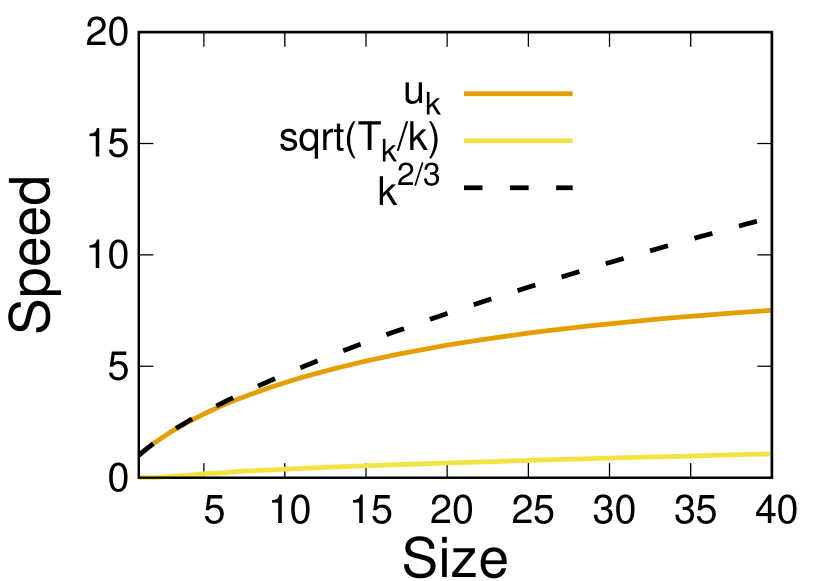
(a)

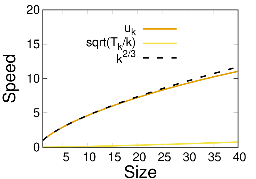
(b)

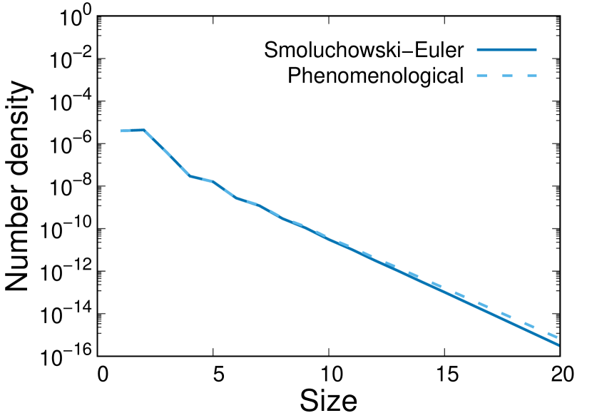
(c)

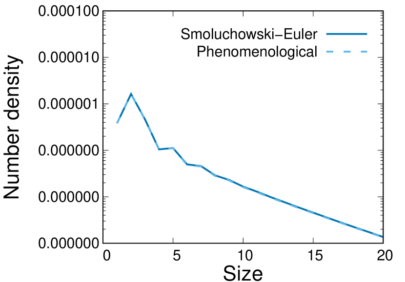
(d)

Figure 1: (a), (b): Partial flow velocities $u_{k}$ of particles of size $k$, and their reduced temperature, $\theta_{k}=T_{k}/k$ ($m_{1}=1$) at $z=-10\,m$ (a) and at $z=-100\,m$ (b). The steady-state velocities $V_{k,\rm eq}=k^{2/3}$ ($V_{\rm 1,eq}=1$) are shown for the approximation, when aggregation is neglected. (c), (d): Comparison of the particles size distribution for the new theory, Eqs. (12)-(14) (full lines), and phenomenological Eq. (2) (dashed lines), with fixed speeds, $u_{k}=k^{2/3}$, directed downward, and kinetic rates, $C_{ij}=\pi\sigma_{ij}^{2}|u_{i}-u_{j}|$, at $z=-10\,m$ (c) and at $z=-100\,m$ (d). The dimensionless monomer source and gravity are $J^{*}=10^{-5}$ and $g^{*}=6.8\times 10^{-3}$. The source of monomers and dimers is located at $z=0$.

Explosion with aggregation. Another important example is the aggregation kinetics in a system of particles (debris), emerging in an explosion, with the center at $r=0$. We consider the spherically symmetric case and neglect all components of the particles’ velocities except the radial one. That is, we assume that $u_{k}=u_{r,k}$ and similarly, $\theta_{k}=\langle(v_{r,k}-u_{k})^{2}\rangle$. Moreover, we neglect gravity and assume that the explosion occurs in vacuum. Then the governing equations read:

$$\frac{\partial}{{\partial t}}{n_{k}}+\frac{1}{r^{2}}\frac{\partial}{\partial r}\left(r^{2}{n_{k}u_{k}}\right)=S_{1},$$ (15)

$$\frac{\partial}{{\partial t}}\left({n_{k}}{u_{k}}\right)+\frac{1}{r^{2}}\frac{\partial}{\partial r}\left(r^{2}n_{k}\left(u_{k}^{2}+\theta_{k}\right)\right)=S_{2,r},$$ (16)

$$\frac{\partial}{{\partial t}}\left({n_{k}}{\theta_{k}}\right)+\frac{1}{r^{2}}\frac{\partial}{\partial r}\left(r^{2}n_{k}u_{k}\theta_{k}\right)=S_{3}.$$ (17)

In $S_{1}$, $\vec{S}_{2}$ and $S_{3}$ we use the same kinetic coefficients as for the quasi-one dimensional case discussed above. For the initial conditions, we assume that at $r=r_{0}=1$ the number density of monomers is $n_{1}(r_{0})=1$, they have average (radial) velocity $u_{0}=1$ with the dispersion $\theta_{0}=0.2$; the initial monomer radial velocities have the Maxwell distribution.

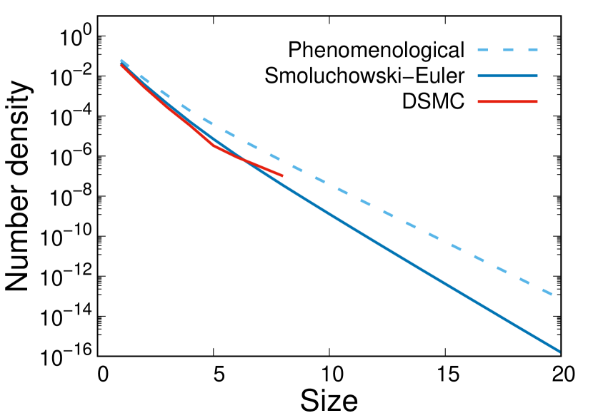
(a)

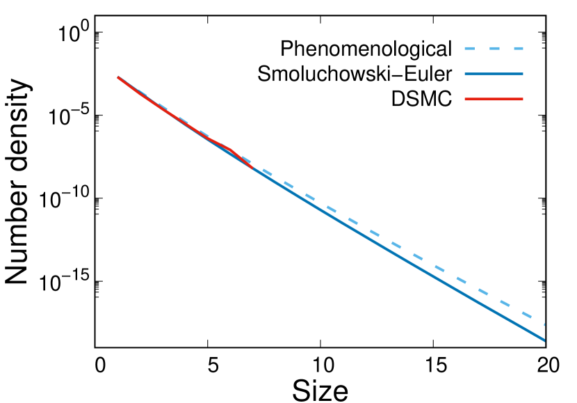
(b)

Figure 2: The size distribution of the aggregates at time $t=2$ for the distances from the epicenter, equal to $r=1$ (a) and $r=4$ (b). The results for the phenomenological model, Eqs. (2) and (18) (dashed lines) are compared with the solution of the Smoluchowski-Euler equations (15)-(17) and DSMC simulation under Maxwell distribution assumption nature with $10^{7}$ initial particles (full lines). At $t=0$ there were only monomers at $r=1$ with the average radial velocity $u_{0}=1$ and dispersion $\theta_{0}=0.2$.

In Fig. 2 we present the size distribution of particles at different radial distances, $r=1$ and $r=4$, at time $t=2$ after the explosion. Here we compare the results, obtained from the solution of the Smoluchowski-Euler equations, (15)-(17) and from the solution of the phenomenological equations (2), supplemented by Euler equations for the flow velocities,

$$\frac{\partial u_{k}}{\partial t}+u_{k}\frac{\partial u_{k}}{\partial r}+\frac{1}{n_{k}r^{2}}\frac{\partial}{\partial r}\left(r^{2}n_{k}\theta_{k}\right)=0,$$ (18)

and fixed temperatures $T_{k}=k\theta_{0}=\mathrm{const}$. Although the aggregation does not affect significantly the flow velocities here (which remain almost equal), the size distribution obtained from Eqs. (15)-(17) of the new theory and phenomenological theory noticeably differ, especially for large aggregates (note that plots have logarithmic scale). The total number density, $N=\sum_{k}n_{k}$, differ however not so much – the observed difference is about $20\%$. We expect, however, that in the course of time the predictions of the phenomenological theory will deviate more and more from the results of the first-principle theory reported here.

Conclusion. We report Smoluchowski-Euler equations, which describe aggregation kinetics in space-inhomogeneous systems with fluxes. We derive these equations for the number density of aggregates, their average velocity and kinetic temperature from the first principles, starting from the Boltzmann equation, and obtain microscopic expression for the aggregation rate coefficients. These coefficients significantly differ from the respective coefficients for homogeneous systems, without fluxes and from their phenomenological generalization. Surprisingly, we reveal, that apart from the conventional aggregation rate coefficients for the cluster densities, a set of new kinetic coefficients appear in the equations for the average velocity and temperature. We also obtain the microscopic expressions for the new kinetic coefficients, which we call “flux-reaction” and “energy-reaction” rates. We consider two representative examples of the application of the new equations – the sedimentation of aggregating particles and aggregation of particles in an explosion. We demonstrate that the results of the new theory significantly differ from the results of the existing phenomenological theory. This indicates that the phenomenological description of the aggregation processes in non-homogeneus systems with fluxes is not reliable, and one needs to apply a new theory, based on the first-principle Smoluchowski-Euler equations reported here. Since the new theory is based on the Boltzmann equations, its application is limited to the aggregating gases. Derivation of the Smoluchowski-Euler equations for dense media remains a challenge for future studies.

Appendix A Boltzmann equation

Consider the case, when the system can be approximated by discretely sized clusters with mass $m_{i}=im_{1}$, with $m_{1}=1$. Then the velocity distributions $f_{k}\left(\vec{V}_{k},\vec{r},t\right)$ for each cluster size $k$, obey the following system of Boltzmann equations

$$\frac{d}{dt}f_{k}\left(\vec{V}_{k}\right)=\frac{1}{2}\sum\limits_{i+j=k}I_{ij}^{{\rm agg},1}\left(\vec{V}_{k}\right)-\sum\limits_{j=1}^{\infty}I_{kj}^{{\rm agg},2}\left(\vec{V}_{k}\right)-\sum\limits_{j=1}^{\infty}I_{kj}^{{\rm res},1}\left(\vec{V}_{k}\right)+\sum\limits_{j=1}^{\infty}I_{kj}^{{\rm res},2}\left(\vec{V}_{k}\right)+{\cal J}_{k}\left(\vec{V}_{k}\right),$$ (19)

where we skip the dependence on $\vec{r}$ and $t$ and ${\cal J}_{k}\left(\vec{V}_{k}\right)$ describes the source of particles of size $k$ and velocity $\vec{V}_{k}$. We also have the following Boltzmann collision integrals, which account for aggregative and restitutive collisions, which we write as $I_{ij}^{{\rm res}}=I_{ij}^{{\rm res},2}-I_{ij}^{{\rm res},1}$:

$$I_{ij}^{{\rm agg},1}\left(\vec{V}_{i+j}\right) =\sigma_{ij}^{2}\iiint\left|\left(\vec{V}_{i}-\vec{V}_{j}\right)\cdot\vec{e}\right|\Theta\left(-\left(\vec{V}_{i}-\vec{V}_{j}\right)\cdot\vec{e}\right)\Theta\left(W_{ij}-\frac{m_{i}m_{j}\left|\vec{V}_{i}-\vec{V}_{j}\right|^{2}}{2\left(m_{i}+m_{j}\right)}\right)$$ (20)

$$\times\delta\left(\vec{V}_{i+j}-\frac{m_{i}\vec{V}_{i}+m_{j}\vec{V}_{j}}{m_{i}+m_{j}}\right)f_{i}\left(\vec{V}_{i}\right)f_{j}\left(\vec{V}_{j}\right)\,d\vec{v}_{i}\,d\vec{v}_{j}\,d\vec{e},$$

$$I_{ij}^{{\rm agg},2}\left(\vec{V}_{i}\right) =\sigma_{ij}^{2}\iint\left|\left(\vec{V}_{i}-\vec{V}_{j}\right)\cdot\vec{e}\right|\Theta\left(-\left(\vec{V}_{i}-\vec{V}_{j}\right)\cdot\vec{e}\right)\Theta\left(W_{ij}-\frac{m_{i}m_{j}\left|\vec{V}_{i}-\vec{V}_{j}\right|^{2}}{2\left(m_{i}+m_{j}\right)}\right)$$

$$\times f_{i}\left(\vec{V}_{i}\right)f_{j}\left(\vec{V}_{j}\right)\,d\vec{v}_{i}\,d\vec{e},$$

$$I_{ij}^{{\rm res},1}\left(\vec{V}_{i}\right) =\sigma_{ij}^{2}\iiint\left|\left(\vec{V}_{i}-\vec{V}_{j}\right)\cdot\vec{e}\right|\Theta\left(-\left(\vec{V}_{i}-\vec{V}_{j}\right)\cdot\vec{e}\right)\Theta\left(\frac{m_{i}m_{j}\left|\vec{V}_{i}-\vec{V}_{j}\right|^{2}}{2\left(m_{i}+m_{j}\right)}-W_{ij}\right)$$

$$\times f_{i}\left(\vec{V}_{i}\right)f_{j}\left(\vec{V}_{j}\right)\,d\vec{v}_{j}\,d\vec{e},$$

$$I_{ij}^{{\rm res},2}\left(\vec{V}_{i}\right) =\sigma_{ij}^{2}\iiint\left|\left(\vec{V}_{i}-\vec{V}_{j}\right)\cdot\vec{e}\right|\Theta\left(-\left(\vec{V}_{i}-\vec{V}_{j}\right)\cdot\vec{e}\right)\Theta\left(\frac{m_{i}m_{j}\left|\vec{V}_{i}-\vec{V}_{j}\right|^{2}}{2\left(m_{i}+m_{j}\right)}-W_{ij}\right)$$

$$\times\frac{1}{\varepsilon^{2}}f_{i}\left(\vec{V}_{i}-\frac{1+\varepsilon}{2\varepsilon}\cdot\frac{m_{j}}{m_{i}+m_{j}}\left(\left(\vec{V}_{i}-\vec{V}_{j}\right)\cdot\vec{e}\right)\vec{e}\right)$$

$$\times f_{j}\left(\vec{V}_{j}+\frac{1+\varepsilon}{2\varepsilon}\cdot\frac{m_{i}}{m_{i}+m_{j}}\left(\left(\vec{V}_{i}-\vec{V}_{j}\right)\cdot\vec{e}\right)\vec{e}\right)d\vec{v}_{j}\,d\vec{e}.$$

Here we introduce the radius of the collision cylinder $\sigma_{ij}$ and the potential barrier $W_{ij}$, which can be used to determine, whether a collision leads to aggregation or bouncing SpahnetalEPL:2004 ; constt1 ; PNAS ; nature . $\Theta$ is the Heaviside unit step function. These functions in the integrands of the above equations select only approaching particles and distinguish between bouncing and aggregating collisions for the particular aggregation barrier $W_{ij}$. That is, if the relative kinetic energy at the very end of a collision, $\varepsilon^{2}m_{i}m_{j}(\vec{V}_{i}-\vec{V}_{j})^{2}/2(m_{i}+m_{j})$, is smaller than the potential barrier energy, the particles merge. Otherwise, they bounce off. The rescaling of the kinetic energy due to inelastic collision can be incorporated into $W_{ij}$, so that, in general, it also depends on the restitution coefficient $\varepsilon$. The unit vector $\vec{e}$ specifies the collision geometry – it is directed along the inter-particle centers at the collision instant. $\vec{V}_{i}$ and $\vec{V}_{j}$ denote the velocities of the colliding particles.

The first aggregation integral describes the rate of change of the distribution function for clusters of size $k=i+j$, emerging in the collisions of clusters of size $i$ and $j$. The second one quantifies the rate of change of the number of clusters of size $i$ with velocities $\vec{V}_{i}$, which disappear in aggregative collisions. The restitution integral $I_{ij}^{{\rm res},2}$ accounts for the amount of clusters that change their velocity from $\vec{V}_{i}$ to $\vec{V}_{i}^{\prime}$ after the collision,

$$\vec{V}_{i/j}^{\prime}=\vec{V}_{i/j}\mp\frac{1+\varepsilon}{2}\cdot\frac{m_{i}}{(m_{i}+m_{j})}\left(\vec{V}_{ij}\cdot\vec{e}\right)\vec{e}.$$

$I_{ij}^{{\rm res},1}$ describes, respectively, the “inverse” collisions with the velocities

$$\vec{V}_{i/j}^{\prime\prime}=\vec{V}_{i/j}\mp\frac{1+\varepsilon}{2\varepsilon}\cdot\frac{m_{i}}{(m_{i}+m_{j})}\left(\vec{V}_{ij}\cdot\vec{e}\right)\vec{e},$$

which end up with the velocities $\vec{V}_{i/j}$. The length of the collision cylinder for the inverse collisions is rescaled accordingly by a factor of $1/\varepsilon^{2}$, see analyticbrill for more detail.

The full time derivative for each size $k$ can be written as follows:

$$\frac{d}{dt}f_{k}\left(\vec{V}_{k},\vec{r},t\right)=\left(\frac{\partial}{\partial t}+\vec{V}_{k}\cdot\frac{\partial}{\partial\vec{r}}+\frac{\vec{F}_{k}}{m_{k}}\cdot\frac{\partial}{\partial\vec{V}_{k}}\right)f_{k}\left(\vec{V}_{k},\vec{r},t\right),$$ (21)

where $\vec{F}_{k}$ is the external force. Here we explicitly state that the velocity distribution can vary in time and space.

The source of particles, used in the main text (monomers and dimers added at $z=0$ with their equilibrium sedimentation velocities) reads,

$${\cal J}(\vec{V}_{k})=J\delta(z)\left[\delta_{k,1}(\vec{V}_{1}-\vec{V}_{\rm eq,1})+\delta_{k,1}(\vec{V}_{2}-\vec{V}_{\rm eq,2})\right]$$

Our extensive Monte Carlo simulations have demonstrated that for an aggregating system, the velocity distribution function for all clusters is very close to Maxwellian, except for a small region for clusters with almost vanishing velocity, see Fig. 3 and the discussion below. Therefore, similarly as in our previous studies, SpahnetalEPL:2004 ; constt1 ; PNAS ; nature , we approximate the velocity distribution function for each individual species by the corresponding Maxwell distribution,

$$f_{k}\left(\vec{V}_{k}\right)=\frac{n_{k}}{\left(2\pi\theta_{k}\right)^{3/2}}e^{\frac{\left(\vec{V}_{k}-\vec{u}_{k}\right)^{2}}{2\theta_{k}}},$$ (22)

where $n_{k}(x,t)=\int f_{k}\left(\vec{V}_{k},\vec{x},t\right)d\vec{V}_{k}$ is the number density of clusters of size $k$, $\vec{u}_{k}=n_{k}^{-1}\int\vec{V}_{k}f_{k}d\vec{V}_{k}$ is the flux velocity of such clusters, and $\theta_{k}=\tfrac{1}{3}n_{k}^{-1}\int(\vec{V}_{k}-\vec{u}_{k})^{2}f_{k}d\vec{V}_{k}$ is their reduced temperature. Note that the scaled “granular” temperatures $\theta_{k}$ describe the speed variance for each distribution $f_{k}$ granmix2 ; bodrova2014 ; the average temperature of the whole system is defined as $T=\sum\limits_{k}n_{k}T_{k}/\sum\limits_{k}n_{k}$.

Appendix B Derivation detail of Smoluchowski-Euler equations for all-aggregative collisions

We start from the simplified case when all collisions are aggregative, which correspond to the case of very large adhesive barrier, $W_{ij}/k_{B}T\to\infty$ for all $k$. In this case, one can neglect the restitution integrals, $I_{ij}^{{\rm res},1}=I_{ij}^{{\rm res},2}=0$. Integrating equations (19) over the velocity $\vec{V}_{k}$, with the use of the distribution (22) we arrive at the Smoluchowski equations for space-inhomogeneous system,

$$\frac{\partial}{\partial t}n_{k}+\vec{\nabla}\left(n_{k}\vec{u}_{k}\right)=\frac{1}{2}\sum\limits_{i+j=k}C_{ij}n_{i}n_{j}-\sum\limits_{j=1}^{\infty}C_{kj}n_{k}n_{j},\qquad\qquad\qquad\qquad\quad\qquad\qquad\qquad\qquad\quad k=\overline{1,\infty}.$$ (23)

Similarly, multiplying Eqs. (19) with the velocity $\vec{V}_{k}$, and then with the square of the local velocity, $\tfrac{1}{3}\vec{v}_{k}^{2}=\tfrac{1}{3}\left|\vec{V}_{k}-\vec{u}_{k}\right|^{2}$, and integrating over $\vec{V}_{k}$, we obtain,

$$\frac{\partial}{\partial t}\left(n_{k}\vec{u}_{k}\right)+n_{k}\vec{u}_{k}\cdot\vec{\nabla}\vec{u}_{k}+\vec{u}_{k}\vec{\nabla}\cdot\left(n_{k}\vec{u}_{k}\right)+\vec{\nabla}\left(n_{k}\theta_{k}\right)-\frac{\vec{F}_{k}}{m_{k}}n_{k}=\frac{1}{2}\sum\limits_{i+j=k}\vec{P}_{ij}n_{i}n_{j}-\sum\limits_{j=1}^{\infty}\vec{R}_{kj}n_{k}n_{j},\quad k=\overline{1,\infty},$$ (24)

$$\frac{\partial}{\partial t}\left(n_{k}\theta_{k}\right)+\vec{\nabla}\cdot\left(n_{k}\theta_{k}\vec{u}_{k}\right)=\frac{1}{2}\sum\limits_{i+j=k}B_{ij}n_{i}n_{j}-\sum\limits_{j=1}^{\infty}D_{kj}n_{k}n_{j},\qquad\qquad\qquad\quad\qquad\qquad\qquad\qquad k=\overline{1,\infty}.$$ (25)

We can call the system (23)-(25) the Smoluchowski-Euler equations. Indeed, when aggregation and energy loss is lacking, the r.h.s disappear, and they convert into Euler equations for the multicomponent molecular gas. For granular gases one needs to keep $I_{ij}^{{\rm res},1/2}$ which results in additional dissipation term in Eq. (25). In the lack of currents, Eq. (23) converts to Smoluchowski equation, if we neglect variation of species temperature; otherwise it converts into temperature-dependent Smoluchowski equations OsBrilJPA2022 ; OsBrilPRE2022 ; gen-smol .

Surprisingly, a set of new kinetic coefficients appear – the vectorial $\vec{P}_{ij}$ and $\vec{R}_{ij}$ and scalar – $B_{ij}$ and $D_{ij}$ (see the derivation below). They reflect the aggregation kinetics in the presence of currents and hence may be dubbed as ”flux-reaction” and ”energy-reaction” rates. Since all the kernels $C_{ij}$, $\vec{P}_{ij}$, $\vec{R}_{ij}$, $B_{ij}$ and $D_{ij}$ in (24)-(25) can be found analytically, we have a closed set for $n_{k}$, $\vec{u}_{k}$ and $T_{k}$, that can be numerically solved, similarly as classical Smoluchowski equations.

If the flow speeds and temperatures are the same for all sizes, and all collisions lead to aggregation, we get the standard ballistic kernel equaltemporig ; constt1 :

$$C_{ij}=2\sqrt{2\pi}\sigma_{ij}^{2}\sqrt{\frac{T}{i}+\frac{T}{j}}.$$

If not all collisions are aggregative and not all temperatures are equal (although all flow speeds are still the same), the above relation generalizes to,

$$C_{ij}=2\sqrt{2\pi}\sigma_{ij}^{2}\sqrt{\frac{T_{i}}{i}+\frac{T_{j}}{j}}p_{ij}\left(T_{i},T_{j}\right),$$

where $p_{ij}(T_{i},T_{j})$ is the aggregation probability, which can be found explicitly nature . This probability is also sometimes called coagulation efficiency atmos .

To obtain the left-hand side (l.h.s.) of Eq. (23), we make the following transformations (below we assume that $\vec{F}_{k}$ does not depend on $\vec{V}_{k}$):

$$\int\left(\frac{\partial}{\partial t}+\vec{V}_{k}\cdot\frac{\partial}{\partial\vec{r}}+\frac{\vec{F}_{k}}{m_{k}}\cdot\frac{\partial}{\partial\vec{V}_{k}}\right)f_{k}d\vec{V}_{k}=\frac{\partial}{\partial t}\int f_{k}d\vec{V}_{k}+\frac{\partial}{\partial\vec{r}}\cdot\int\vec{V}_{k}f_{k}d\vec{V}_{k}+\frac{\vec{F}_{k}}{m_{k}}\int\frac{\partial}{\partial\vec{V}_{k}}f_{k}d\vec{V}_{k}=\frac{\partial n_{k}}{\partial t}+\vec{\nabla}\cdot(n_{k}\vec{u}_{k})+0,$$

where we use the definition of $n_{k}$ and $\vec{u}_{k}$. Similarly, we obtain the $\beta$-component ($\alpha,\beta=x,y,z$) of the l.h.s. of Eq. (24), using the summation convention and $\vec{v}_{k}=\vec{V}_{k}-\vec{u}_{k}$,

$$\int V_{k,\beta}\left(\frac{\partial}{\partial t}+V_{k,\alpha}\frac{\partial}{\partial r_{\alpha}}+\frac{F_{k,\alpha}}{m_{k}}\cdot\frac{\partial}{\partial V_{k,\alpha}}\right)f_{k}d\vec{V}_{k}$$

$$~{}~{}~{}=\frac{\partial}{\partial t}\int V_{k,\beta}f_{k}d\vec{V}_{k}+\frac{\partial}{\partial r_{\alpha}}\int V_{k,\alpha}V_{k,\beta}f_{k}d\vec{V}_{k}+\frac{F_{k,\alpha}}{m_{k}}\int V_{k,\beta}\frac{\partial}{\partial V_{k,\alpha}}f_{k}d\vec{V}_{k}$$

$$~{}~{}~{}=\frac{\partial}{\partial t}(n_{k}u_{k,\beta})+\frac{\partial}{\partial r_{\alpha}}\int(v_{k,\alpha}+u_{k,\alpha})(v_{k,\beta}+u_{k,\beta})f_{k}d\vec{V}_{k}-\frac{F_{k,\alpha}}{m_{k}}\delta_{\alpha,\beta}\int f_{k}d\vec{V}_{k}$$

$$~{}~{}~{}=\frac{\partial}{\partial t}(n_{k}u_{k,\beta})+\frac{\partial}{\partial r_{\alpha}}\delta_{\alpha,\beta}\int v_{k,\beta}v_{k,\alpha}f_{k}d\vec{V}_{k}+\frac{\partial}{\partial r_{\alpha}}(u_{k,\beta}u_{k,\alpha}n_{k})-\frac{F_{k,\beta}}{m_{k}}n_{k}$$

$$~{}~{}~{}=\frac{\partial}{\partial t}(n_{k}u_{k,\beta})+\frac{\partial}{\partial r_{\beta}}n_{k}\theta_{k}+u_{k,\beta}\vec{\nabla}\cdot(n_{k}\vec{u}_{k})+n_{k}(\vec{u}_{k}\cdot\vec{\nabla})u_{k,\beta}-\frac{F_{k,\beta}}{m_{k}}n_{k}.$$ (26)

Here we also used $\int(v_{k,\alpha})^{n}f_{k}d\vec{V}_{k}=0$ for odd $n$. For the l.h.s. of Eq. (25) we find:

$$\int\frac{v_{k}^{2}}{3}\left(\frac{\partial}{\partial t}+V_{k,\alpha}\frac{\partial}{\partial r_{\alpha}}+\frac{F_{k,\alpha}}{m_{k}}\cdot\frac{\partial}{\partial V_{k,\alpha}}\right)f_{k}d\vec{V}_{k}$$

$$~{}~{}~{}=\frac{\partial}{\partial t}\int\frac{v_{k}^{2}}{3}f_{k}d\vec{V}_{k}+\frac{\partial}{\partial r_{\alpha}}\int\frac{v_{k}^{2}}{3}(v_{k,\alpha}+u_{k,\alpha})f_{k}d\vec{V}_{k}+\frac{F_{k,\alpha}}{m_{k}}\int\frac{v_{k}^{2}}{3}\frac{\partial}{\partial V_{k,\alpha}}f_{k}d\vec{V}_{k}$$

$$~{}~{}~{}=\frac{\partial}{\partial t}(n_{k}\theta_{k})+\frac{\partial}{\partial r_{\alpha}}u_{k,\alpha}\int\frac{v_{k}^{2}}{3}f_{k}d\vec{V}_{k}-\frac{F_{k,\alpha}}{m_{k}}\int\left(\frac{\partial}{\partial V_{k,\alpha}}\frac{v_{k}^{2}}{3}\right)f_{k}d\vec{V}_{k}$$

$$~{}~{}~{}=\frac{\partial}{\partial t}(n_{k}\theta_{k})+\vec{\nabla}\cdot(n_{k}\theta_{k}\vec{u}_{k}).$$ (27)

In the case when the external force depends on the velocity $\vec{V}_{k}$, that is, $\vec{F}_{k}=\vec{h}_{k}(\vec{V}_{k})$, the last term in Eq. (21) should be written as $\partial/\partial\vec{V}_{k}\cdot(f_{k}\vec{F}_{k}/m_{k})$. Then the last term in the r.h.s. of Eq. (B) takes the form $-\int f_{k}\vec{h}_{k}\cdot d\vec{V}_{k}$, or $3\pi\eta\sigma_{k}n_{k}\vec{u}_{k}/m_{k}$, when $\vec{F}_{k}$ obeys the Stokes law. Similarly, in the r.h.s. of Eq. (B) appears an additional term, $6\pi\eta\sigma_{k}n_{k}\theta_{k}/m_{k}$, if $\vec{F}_{k}$ follows the Stokes law.

Turn now to the derivation of the r.h.s. of Eqs. (23)-(25), which implies the derivation of the respective kinetic coefficients.

Appendix C Derivation of the kinetic coefficient for all-merging collisions

C.1 3D case

Let us derive the kernels (i.e. the transport- reactive coefficients) for the case, when all collisions are merging. Here we present the detailed, step-by-step derivation for the kinetic coefficients $C_{ij}$; all other kinetic coefficients $\vec{P}_{ij}$, $\vec{R}_{ij}$, $B_{ij}$ and $D_{ij}$ may be derived analogously.

First, we notice that the following relation holds true,

$$C_{ij}n_{i}n_{j}=\int I_{ij}^{{\rm agg},2}\,d\vec{v}_{i},$$ (28)

that is, we need to integrate over all speeds to find the total number of collisions, which, in our case, is the same as the total number of aggregating collisions. Here $\vec{v}_{i}$, as before, is the “local” speed of size-$i$ particles – the speed in the system of coordinates moving with their flux velocity $\vec{u}_{i}$. Hereinafter, we will use $m_{i}=i$. To simplify the computations, we introduce the scaled temperatures $\theta_{i}=T_{i}/i$.

We start with the change of variables in $I_{ij}^{{\rm agg},2}$ from $\vec{v}_{i}$ and $\vec{v}_{j}$ to

$$\vec{w} =\vec{v}_{i}-\vec{v}_{j},$$

$$\vec{u} =\frac{\theta_{j}\vec{V}_{i}+\theta_{i}\vec{V}_{j}}{\theta_{i}+\theta_{j}},$$

and denote

$$\vec{W}=\vec{V}_{i}-\vec{V}_{j}.$$

Substituting the Maxwell distribution and using the new variables yields,

$$C_{ij}=\frac{\sigma_{ij}^{2}}{\left(2\pi\right)^{3}\theta_{i}^{3/2}\theta_{j}^{3/2}}\iiint d\vec{w}\,d\vec{u}\,d\vec{e}\,\theta\left(-\vec{W}\cdot\vec{e}\right)\left|\vec{W}\cdot\vec{e}\right|e^{-\frac{u^{2}}{2}\left(\theta_{i}^{-1}+\theta_{j}^{-1}\right)-\frac{w^{2}}{2\left(\theta_{i}+\theta_{j}\right)}}.$$

The above integral is Gaussian with respect to $\vec{u}$ and hence may be easily calculated, with the result:

$$C_{ij}=\frac{\sigma_{ij}^{2}}{\left(2\pi\right)^{3/2}\left(\theta_{i}+\theta_{j}\right)^{3/2}}\iint d\vec{w}\,d\vec{e}\,\theta\left(-\vec{W}\cdot\vec{e}\right)\left|\vec{W}\cdot\vec{e}\right|e^{-\frac{w^{2}}{2\left(\theta_{i}+\theta_{j}\right)}}.$$

Integration over the unit vector $\vec{e}$ (actually only over the semi-sphere) may be also easily performed, (see e.g. Ref. BrilliantovPoeschelOUP where such integrals are evaluated). With the obvious notation for vectors moduli, $W=\left|\vec{W}\right|$, we arrive at:

$$C_{ij}=\frac{\pi\sigma_{ij}^{2}}{\left(2\pi\right)^{3/2}\left(\theta_{i}+\theta_{j}\right)^{3/2}}\int d\vec{w}\,We^{-\frac{w^{2}}{2\left(\theta_{i}+\theta_{j}\right)}}.$$

Next, we make another change of variables $\vec{v}=\vec{W}/\sqrt{2\left(\theta_{i}+\theta_{j}\right)}$ and denote

$$\vec{c}=\sqrt{\frac{2}{\theta_{i}+\theta_{j}}}\left(\vec{u}_{i}-\vec{u}_{j}\right).$$

Then

$$C_{ij}=\sqrt{\frac{2}{\pi}}\sigma_{ij}^{2}\sqrt{\theta_{i}+\theta_{j}}\int d\vec{v}\,ve^{-\left|\vec{v}-\frac{\vec{c}}{2}\right|^{2}}.$$

Changing to the cylindrical coordinates $\left(h,r,\phi\right)$, where $h$ is the coordinate for the axis, directed along $\vec{c}$, and integrating over the angle $\varphi$ we obtain:

$$C_{ij}=2\sqrt{2\pi}\sigma_{ij}^{2}\sqrt{\theta_{i}+\theta_{j}}\int_{-\infty}^{\infty}dh\int_{0}^{\infty}dr\,\sqrt{r^{2}+h^{2}}e^{-r^{2}-\left|h-\frac{c}{2}\right|^{2}}.$$

Now we change the variable in the second integral as $R=r^{2}+h^{2}$ and integrate by parts

$$C_{ij} =\sqrt{2\pi}\sigma_{ij}^{2}\sqrt{\theta_{i}+\theta_{j}}\int_{-\infty}^{\infty}dh\int_{h^{2}}^{\infty}dR\,\sqrt{R}e^{h^{2}-R-\left|h-\frac{c}{2}\right|^{2}}$$

$$=2\sqrt{2\pi}\sigma_{ij}^{2}\sqrt{\theta_{i}+\theta_{j}}\int_{-\infty}^{\infty}\frac{h\left|h\right|}{c}e^{-h^{2}+ch-c^{2}/4}\,dh.$$

The above integral may be written as a sum of two parts, corresponding to the different signs of $h$, as:

$$C_{ij}=2\sqrt{2\pi}\sigma_{ij}^{2}\sqrt{\theta_{i}+\theta_{j}}\left(\int_{0}^{\infty}\frac{h^{2}}{c}e^{-h^{2}-ch-c^{2}/4}\,dh+\int_{0}^{\infty}\frac{h^{2}}{c}e^{-h^{2}+ch-c^{2}/4}\,dh\right).$$

After the change of variables $z=h-c/2$, both integrals will turn into a combination of incomplete Gamma functions of an integer argument, yielding finally the result

$$C_{ij}=\sqrt{2\pi}\sigma_{ij}^{2}\sqrt{\theta_{i}+\theta_{j}}\left[e^{-c^{2}/4}+\frac{\sqrt{\pi}(c^{2}+2)}{2c}{\rm erf}(\tfrac{c}{2})\right],$$ (29)

$$c=\sqrt{\frac{2}{\theta_{i}+\theta_{j}}}\left|\vec{u}_{i}-\vec{u}_{j}\right|.$$

Though it is undefined for $\vec{u}_{i}=\vec{u}_{j}$, i.e., for $c=0$, the corresponding value can still be found in the limit $c\to+0$. Using the same steps as for the derivation of $C_{ij}$, we find all other kinetic coefficients:

$$\vec{P}_{ij} =C_{ij}\vec{\mu}+2\sqrt{2\pi}\sigma_{ij}^{2}q\vec{c}\left(e^{-c^{2}/4}\left(1/c^{2}+6\right)+\frac{\sqrt{\pi}}{2c}\left(1-2/c^{2}\right){\rm erf}\left(c/2\right)\right),$$

$$\vec{R}_{ij} =C_{ij}\vec{u}_{i}+2\sqrt{2\pi}\sigma_{ij}^{2}\theta_{i}\vec{c}\left(e^{-c^{2}/4}\left(1/c^{2}+6\right)+\frac{\sqrt{\pi}}{2c}\left(1-2/c^{2}\right){\rm erf}\left(c/2\right)\right),$$

$$B_{ij} =C_{ij}\left(\left|\vec{\mu}-\vec{u}_{i+j}\right|^{2}/3+\frac{\theta_{i}\theta_{j}}{\theta_{i}+\theta_{j}}-\frac{q}{3\left(\theta_{i}+\theta_{j}\right)}\left(\vec{u}_{i}-\vec{u}_{j}\right)\cdot\left(\vec{\mu}-\vec{u}_{i+j}\right)\right)$$

$$+\frac{2}{3}\sqrt{2\pi}\sigma_{ij}^{2}\sqrt{\theta_{i}+\theta_{j}}qI_{B}\left|\vec{\mu}-\vec{u}_{i+j}\right|/\left|\vec{u}_{i}-\vec{u}_{j}\right|$$

$$+\sqrt{2\pi}\sigma_{ij}^{2}q^{2}\left(e^{-c^{2}/4}+\frac{\sqrt{\pi}}{6c}\left(10+3c^{2}\right){\rm erf}\left(c/2\right)\right)/\sqrt{\theta_{i}+\theta_{j}},$$

$$D_{ij} =C_{ij}\frac{\theta_{i}\theta_{j}}{\theta_{i}+\theta_{j}}+\sqrt{2\pi}\sigma_{ij}^{2}\frac{\theta_{i}^{2}}{\sqrt{\theta_{i}+\theta_{j}}}\left(e^{-c^{2}/4}+\frac{\sqrt{\pi}}{6c}\left(10+3c^{2}\right){\rm erf}\left(c/2\right)\right),$$

$$I_{B} =\frac{\sqrt{\pi}}{8}\left(c^{3}+4c-4/c\right){\rm erf}\left(c/2\right)+\frac{1}{2}e^{-c^{2}/4}+\frac{13}{4}c^{2}e^{-c^{2}/4},$$

$$\vec{\mu} =\frac{i\vec{u}_{i}+j\vec{u}_{j}}{i+j},$$

$$q =\frac{T_{i}-T_{j}}{i+j}.$$

If the particles are spherical and monomers have unit diameter, then ${\sigma_{ij}}=\tfrac{1}{2}(\sigma_{i}+\sigma_{j})=\tfrac{1}{2}(i^{1/3}+j^{1/3})$.

C.2 Quasi-1D case

Previously, we assumed that the speed variance is spherically symmetric $\theta_{k,x}=\theta_{k,y}=\theta_{k,z}$. There exists, however, an important for applications case of quasi-one dimensional motion, when one of the components dominates, e.g. $\theta_{k,z}=\int v_{k,z}^{2}f_{k}\left(\vec{v}_{k},\vec{x},t\right)d\vec{v}_{k}\gg\max\left(\theta_{k,x},\theta_{k,y}\right)$. As an example of such systems, one can mention aggregating particles, freely falling in the air. Generally, the particles experience three forces – the force of gravity (along with the buoyancy), the force of viscous resistance and the stochastic force, due to random collisions of the particles with the molecules of the gas. If the particles are massive enough, one can neglect the stochastic force, as the change of particles’ impulse in the collisions with the gas molecules is negligible. In this case, the lateral motion of particles quickly damped by the air viscosity, while the gravity force supports the vertical motion with a high, but constant, velocity. This makes the motion of the system quasi-one dimensional. The dispersion of the cluster velocities, quantified by the partial temperatures, $T_{k}$, emerge due to collisions between the aggregates.

The derivation of the kinetic coefficients is similar in this case, although the resulting kernels are different. We choose the coordinate system with the vertically directed axis $OZ$. In this case, the horizontal velocity variance is quickly dumped by the air resistance. The same happens with the corresponding flux velocities, so that $u_{i,x}=u_{i,y}=0$ for all $i$. With the notations $V_{k}=V_{k,z}$, $u_{k}=u_{k,z}$ and $\theta_{k}=\theta_{k,z}$, we obtain,

$$f_{k}\left(\vec{V}_{k}\right)\approx\frac{n_{k}}{\left(2\pi\theta_{k}\right)^{1/2}}e^{\frac{\left(V_{k}-\vec{u}_{k}\right)^{2}}{2\theta_{k}}}\delta\left(V_{k,x}\right)\delta\left(V_{k,y}\right).$$

We use similar variables as before, although these are now one-dimensional:

$$w =v_{i}-v_{j},$$

$$u =\frac{\theta_{j}V_{i}+\theta_{i}V_{j}}{\theta_{i}+\theta_{j}},$$

$$W =V_{i}-V_{j}.$$

Substituting the distribution functions into the equation for $C_{ij}$ leads to

$$C^{(1D)}_{ij} =\frac{\sigma_{ij}^{2}}{2\pi\theta_{i}^{1/2}\theta_{j}^{1/2}}\iiint dw\,du\,d\vec{e}\,\theta\left(-\vec{W}\cdot\vec{e}\right)\left|\vec{W}\cdot\vec{e}\right|e^{-\frac{u^{2}}{2}\left(\theta_{i}^{-1}+\theta_{j}^{-1}\right)-\frac{w^{2}}{2\left(\theta_{i}+\theta_{j}\right)}}$$

$$=\frac{\sigma_{ij}^{2}}{\left(2\pi\right)^{1/2}\left(\theta_{i}+\theta_{j}\right)^{1/2}}\iiint dw\,d\vec{e}\,\theta\left(-\vec{W}\cdot\vec{e}\right)\left|\vec{W}\cdot\vec{e}\right|e^{-\frac{w^{2}}{2\left(\theta_{i}+\theta_{j}\right)}}$$

$$=\frac{\pi\sigma_{ij}^{2}}{\left(2\pi\right)^{1/2}\left(\theta_{i}+\theta_{j}\right)^{1/2}}\iiint dw\,\left|W\right|e^{-\frac{w^{2}}{2\left(\theta_{i}+\theta_{j}\right)}}.$$

Integrating in the same way as before, we get the following kernel:

$$C^{(1D)}_{ij}=\sqrt{2\pi}\sigma_{ij}^{2}\sqrt{\theta_{i}+\theta_{j}}e^{-c^{2}/4}+\pi\sigma_{ij}^{2}\left|u_{i}-u_{j}\right|{\rm erf}\left(c/2\right),$$ (30)

$$c=\sqrt{\frac{2}{\theta_{i}+\theta_{j}}}\left|\vec{u}_{i}-\vec{u}_{j}\right|.$$

Other kernels for the quasi-one dimensional case read:

$$P^{(1D)}_{ij} =C_{ij}\mu+\pi\sigma_{ij}^{2}q{\rm erf}\left(c/2\right),$$

$$R^{(1D)}_{ij} =C_{ij}u_{i}+\pi\sigma_{ij}^{2}\theta_{i}{\rm erf}\left(c/2\right),$$

$$B^{(1D)}_{ij} =C_{ij}\left(\left|\vec{\mu}-\vec{u}_{i+j}\right|^{2}+\frac{\theta_{i}\theta_{j}+q^{2}}{\theta_{i}+\theta_{j}}\right)$$

$$+2\pi\left(\mu-u_{i+j}\right)\sigma_{ij}^{2}q{\rm erf}\left(c/2\right)+\sqrt{2\pi}\sigma_{ij}^{2}q^{2}e^{-c^{2}/4}/\sqrt{\theta_{i}+\theta_{j}},$$

$$D^{(1D)}_{ij} =C_{ij}\theta_{i}+\sqrt{2\pi}\sigma_{ij}^{2}\theta_{i}^{2}e^{-c^{2}/4}/\sqrt{\theta_{i}+\theta_{j}},$$

$$\mu =\frac{iu_{i}+ju_{j}}{i+j},$$

$$q =\frac{T_{i}-T_{j}}{i+j}.$$

The terms which stem from the source term ${\cal J}$ in the equations for the quasi-one dimensional case, on the r.h.s. of these equations reads,

$$\int J\delta(z)[\delta_{k,1}\delta(V_{1}-V_{\rm eq,1})+\delta_{k,2}\delta(V_{1}-V_{\rm eq,2})]f_{k}d\vec{V}_{k}=J\delta(z)[\delta_{k,1}+\delta_{k,2}],$$

$$\int J\delta(z)[\delta_{k,1}\delta(V_{1}-V_{\rm eq,1})+\delta_{k,2}\delta(V_{1}-V_{\rm eq,2})]V_{k}f_{k}d\vec{V}_{k}=J\delta(z)[\delta_{k,1}+2^{2/3}\delta_{k,2}],$$

and

$$\int J\delta(z)[\delta_{k,1}\delta(V_{1}-V_{\rm eq,1})+\delta_{k,2}\delta(V_{1}-V_{\rm eq,2})]\tfrac{1}{3}v_{k}^{2}f_{k}d\vec{V}_{k}=0,$$

since we assume that the particles of the source have the same steady velocity, $V_{k}=V_{\rm eq,k}=u_{k}$, which implies $v_{k}=0$.

When we write the Smoluchowski-Euler equations in spherical coordinate, we take into account that the radial component of the gradient of a function $H$ reads $\vec{e}_{r}(\partial H/\partial r)$, while a divergence of a vector $\vec{A}=(A_{r},0,0)$ is $r^{-2}\partial(r^{2}A_{r})/\partial r$.

Let us compare our results with some previous models. We have already seen that it is a direct generalization of the classical ballistic kernel. However, we should also look at the previous attempts to add flow speeds into the equations. In the simplest case, the universal flow speed and temperature can be introduced phenomenologically, like in Ref. proto . The authors write the coagulation kernel as

$$C_{ij}=2\sqrt{2\pi}\sigma_{ij}^{2}\sqrt{\frac{T}{i}+\frac{T}{j}}+\pi\sigma_{ij}^{2}\left|\vec{u}_{i}-\vec{u}_{j}\right|,$$ (31)

just by adding the contributions of flow speed and thermal speed. Naturally, this gives the right prediction, when either flow speed or thermal speed dominates, which is also true for our results, Eq. (29). However, the simple model (31) cannot be used when flow speed differences and thermal speed differences are of the same order. Also, it cannot be used, for granular gases or mixtures of granular and molecular gases, when the temperatures of different species are not the same, or temperatures of granular particles differ from that of molecular gas. This is commonly the case for ballistic aggregation: when there are only a few particles of granular gas, so that their rare collisions do not affect much their temperature; instead they experience Brownian motion in molecular gas. In the case of ballistic motion, granular temperature is much smaller than that of molecular gas, even in non-aggregating granular gases, due to energy loss in their inelastic collisions bodrovamol .

Therefore, new equations reported in the main part of the article solve several problems. They are applicable independently of the ratio of the thermal and flow velocities and can account for the temperature difference of different species, which is a common case in driven granular gases bodrova . They account for the difference between granular temperatures and the temperature of the medium, and they can be used to predict the temperature and flow speed evolution in granular gases, as they change during the aggregation. The correct description of the evolution of the entangled number densities, flow fields and temperatures of different species provide a more accurate prediction for the behavior of the system, as compared to that based on the phenomenological equations, with phenomenological rate coefficients.

Appendix D Details of the numerical scheme

Consider now the numerical analysis of the system (23)-(25). For simplicity, we address the case, where the non-uniformity comes from the $z$-axis, for example, due to the presence of the gravitational force. Then the equations take the form

$$\frac{\partial}{{\partial t}}{n_{k}}+\frac{\partial}{\partial z}\left({n_{k}\vec{u}_{k}}\right)=\frac{1}{2}\sum\limits_{i+j=k}{{C_{ij}}{n_{i}}{n_{j}}}-\sum\limits_{j=1}^{\infty}{{C_{kj}}{n_{k}}{n_{j}}},\quad k=\overline{1,\infty},$$

$$\frac{\partial}{{\partial t}}\left({n_{k}}{u_{k}}\right)+\frac{\partial}{\partial z}\left(n_{k}u_{k}^{2}\right)+\frac{\partial}{\partial z}\left({n_{k}\theta_{k}}\right)+n_{k}g=\frac{1}{2}\sum\limits_{i+j=k}{{P_{ij}}{n_{i}}{n_{j}}}-\sum\limits_{j=1}^{\infty}{{R_{kj}}{n_{k}}{n_{j}}},\quad k=\overline{1,\infty},$$

$$\frac{\partial}{{\partial t}}\left({n_{k}}{\theta_{k}}\right)+\frac{\partial}{\partial z}\left(n_{k}u_{k}\theta_{k}\right)=\frac{1}{2}\sum\limits_{i+j=k}{{B_{ij}}{n_{i}}{n_{j}}}-\sum\limits_{j=1}^{\infty}{{D_{kj}}{n_{k}}{n_{j}}},\quad k=\overline{1,\infty},$$

We can use space discretization in the vertical direction and apply the appropriate boundary conditions. For example, in the case when particles are falling, we should either define the number density, speed and temperatures at the highest point, or put an appropriate source there. We should also limit ourselves to a finite number of equations $N$. After that, we can utilize any appropriate time and space discretization. In the simplest case, we can exploit the forward Euler scheme. Note that we can use a smaller time step or a different scheme for the Smoluchowski equations subsystem (first equations in the above set of equations), if they require a more accurate consideration.

Hence, the simplest time and space discretization reads:

$$n_{k}\left(t=t_{n+1},z=h_{m}\right)=n_{k}\left(t=t_{n},z=h_{m}\right)$$

$$+\left(\left(n_{k}u_{k}\right)\left(t=t_{n},z=h_{m-1}\right)-\left(n_{k}u_{k}\right)\left(t=t_{n},z=h_{m}\right)\right)\Delta t_{n}/h$$

$$+\left(\frac{1}{2}\sum\limits_{i+j=k}{{C_{ij}}{n_{i}}{n_{j}}}-\sum\limits_{j=1}^{\infty}{{C_{kj}(t_{n})}{n_{k}}{n_{j}}}\right)\left(t=t_{n},z=h_{m}\right)\Delta t_{n},\quad k=\overline{1,\infty},$$

$$\left(n_{k}u_{k}\right)\left(t=t_{n+1},z=h_{m}\right)=\left(n_{k}u_{k}\right)\left(t=t_{n},z=h_{m}\right)-n_{k}\left(t=t_{n},z=h_{m}\right)g\Delta t_{n}$$

$$+\left(\left(n_{k}u_{k}^{2}+n_{k}\theta_{k}\right)\left(t=t_{n},z=h_{m-1}\right)-\left(n_{k}u_{k}^{2}+n_{k}\theta_{k}\right)\left(t=t_{n},z=h_{m}\right)\right)\Delta t_{n}/h$$

$$+\left(\frac{1}{2}\sum\limits_{i+j=k}{{P_{ij}}{n_{i}}{n_{j}}}-\sum\limits_{j=1}^{\infty}{{R_{kj}}{n_{k}}{n_{j}}}\right)\left(t=t_{n},z=h_{m}\right)\Delta t_{n},\quad k=\overline{1,\infty},$$

$$\left(n_{k}\theta_{k}\right)\left(t=t_{n+1},z=h_{m}\right)=\left(n_{k}\theta_{k}\right)\left(t=t_{n},z=h_{m}\right)$$

$$+\left(\left(n_{k}u_{k}\theta_{k}\right)\left(t=t_{n},z=h_{m-1}\right)-\left(n_{k}u_{k}\theta_{k}\right)\left(t=t_{n},z=h_{m}\right)\right)\Delta t_{n}/h$$

$$+\left(\frac{1}{2}\sum\limits_{i+j=k}{{B_{ij}}{n_{i}}{n_{j}}}-\sum\limits_{j=1}^{\infty}{{D_{kj}}{n_{k}}{n_{j}}}\right)\left(t=t_{n},z=h_{m}\right)\Delta t_{n},\quad k=\overline{1,\infty},$$

$$h_{m}=-mh,m=\overline{0,m_{\max}},\quad t_{n+1}=t_{n}+\Delta t_{n}.$$

We then used predictor-corrector approach to have second order time discretization, as in gen-smol , where one can find other details for the solution of temperature-dependent Smoluchowski equations. The time step was selected adaptively to be the minimal between the time step, which guarantees stability of temperature-dependent Smoluchowski equations and $\Delta t(t_{n})\leqslant 0.2\Delta h/\max_{k,m}\left|u_{k}\left(t_{n},h_{m}\right)\right|$, which guarantees the stability of the vertical transport modelling. Unfortunately, we cannot generally use a low-rank approximation approach, see e.g. gen-smol , since, when the flow speed difference is large, the elements of $C_{ij}$ do not change smoothly.

Appendix E Closeness of the velocity distribution to the Maxwell distribution

Generally, the Maxwell distribution holds only for systems with bouncing collisions of particles, without energy loss. Inelastic collisions result in deviations from the Maxwell distribution, including the exponential high-velocity tails, e.g. analyticbrill . However, aggregation is not just a special case of inelastic collisions. Intuitively, one can still expect that the Maxwell distribution may remain a good approximation for aggregating systems. Indeed, once the particles aggregated, the speed of the new cluster is the speed of the center of mass of the old pair. And if one takes some sample of random pairs of clusters, with Maxwell distribution, the centers of masses of the pairs will also obey the Maxwell distribution. Hence, the aggregation preserves the form of the Maxwell distribution, provided all clusters have the same temperature. The difference of temperatures may, however, affect the distribution and distort the Maxwellian; still, we expect that the distortion would be small.

To test our hypothesis of closeness between the real velocity distribution during aggregation and the Maxwell distribution, we perform Direct Simulation Monte Carlo dsmc of the space homogeneous system, which obeys the equation (19):

$$\frac{d}{dt}f_{k}\left(\vec{V}_{k}\right)=\sum\limits_{i+j=k}I_{ij}^{{\rm agg},1}\left(\vec{V}_{k}\right)-\sum\limits_{j=1}^{\infty}I_{kj}^{{\rm agg},2}\left(\vec{V}_{k}\right)$$

with all collisions leading to aggregation, $\vec{u}_{k}=0$ for all $k$, monodisperse initial conditions $n_{1}=1$ and $N_{p}=3\cdot 10^{8}$ initial particles with unit diameter and speeds from the Maxwell distribution with initial temperature $T_{1}=1$.

Irreversible aggregation quickly leads to a multi-component system with the so-called scaling distribution of particles sizes scaling . For aggregation described by the Boltzmann equations, the average temperature scales as $T\sim t^{-1/3}$ and typical mass $s$ (scaling parameter) scales as $s=n^{-1}\sim t^{-1}$ equaltemporig . So, at $t=100$ the typical mass in the system is about 100. Figure 3 shows the velocity distribution, obtained by Monte Carlo simulations at that time instant. The figure demonstrates that while the distribution deviates for small clusters from the Maxwellian at small velocities, it is very close to it for large clusters. That is, the clusters of typical mass (about $100$ at $t=100$) or larger have the velocity distribution very close to the Maxwellian. This justifies the assumption of Maxwell distribution exploited in the main text in the derivation of Smoluchowski-Euler equations.

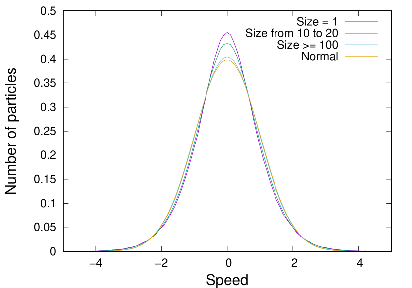
(a) $x$ component of the velocity distribution function at $t=100$ for different sizes, compared to the Maxwellian (normal) distribution. All velocity distributions are rescaled to $T=1$. The typical size of clusters at $t=100$ is about $k=100$.

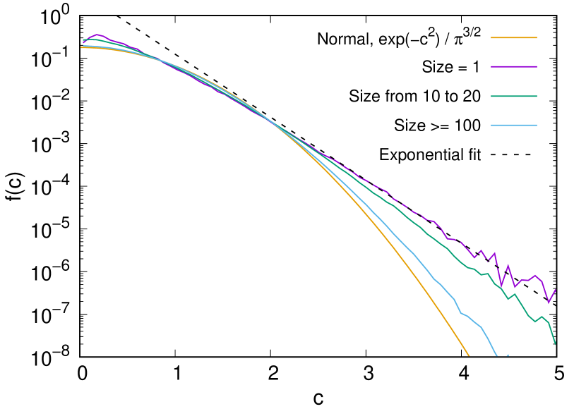
(b) Dimensionless spherically symmetric velocity distribution at $t=100$ for various cluster sizes compared to Maxwell distribution and exponential tail.

Figure 3: Comparison between the Maxwell distribution and velocity distributions observed in Monte Carlo simulations of aggregating system for the initial condition of $10^{8}$monomers.

References

[1]
M. V. Smoluchowski.
Drei vortrage uber diffusion, brownsche bewegung und koagulation von
kolloidteilchen.
Z. Phys., 17:557, 1916.
[2]
Hans Müller.
Zur allgemeinen theorie ser raschen koagulation.
Fortschrittsberichte über Kolloide und Polymere, 27(6):223,
1928.
[3]
M. V. Smoluchowski.
Attempt for a mathematical theory of kinetic coagulation of colloid
solutions.
Z. Phys. Chem., 92:129, 1917.
[4]
S. Chandrasekhar.
Stochastic problems in physics and astronomy.
Rev. Mod. Phys., 15:1, 1943.
[5]
P. L. Krapivsky, A. Redner, and E. Ben-Naim.
A Kinetic View of Statistical Physics.
Cambridge University Press, Cambridge, UK, 2010.
[6]
F. Leyvraz.
Scaling theory and exactly solved models in the kinetics of
irreversible aggregation.
Phys. Reports, 383:95, 2003.
[7]
G. Falkovich, A. Fouxon, and M. Stepanov.
Acceleration of rain initiation by cloud turbulence.
Nature, 419:151, 2002.
[8]
G. Falkovich, M. G. Stepanov, and M. Vucelja.
Rain initiation time in turbulent warm clouds.
Journal of Applied Meteorology and Climatology, 45:591, 2006.
[9]
T. Poeschel, N. V. Brilliantov, and C. Frommel.
Kinetics of prion growth.
Biophysical J., 85:3460, 2003.
[10]
V. J. Anderson and H. N.W. Lekkerkerker.
Insights into phase transition kinetics from colloid science.
Nature, 416:811, 2002.
[11]
A. Stradner, H. Sedgwick, F. Cardinaux, W. C. K. Poon, S. U. Egelhaaf, and
P. Schurtenberge.
Equilibrium cluster formation in concentrated protein solutions and
colloids.
Nature, 432:492, 2004.
[12]
R. W. Samsel and A. S. Perelson.
Kinetics of rouleau formation. i. a mass action approach with
geometric features.
Biophys. J., 37:493, 1982.
[13]
M.A.Anand, K. B. Rajagopal, and K.R. Rajagopal.
A model for the formation and lysis of blood clots.
Pathophysiology of Haemostasis and Thrombosis, 34:109, 2005.
[14]
S. K. Friedlander.
Smoke, Dust and Haze.New York: Wiley Interscience, 1997.
[15]
J. H. Seinfeld and S. N. Pandis.
Atmospheric Chemistry and Physics.
Wiley, New York, 1998.
[16]
N.V. Brilliantov, P.L. Krapivsky, A.S. Bodrova, F. Spahn, H. Hayakawa,
V. Stadnichuk, and J. Schmidt.
Size distribution of particles in saturn’s rings from aggregation and
fragmentation.
PNAS, 112(31):9536–9541, 2015.
[17]
N.V. Brilliantov, A.S. Bodrova, and P.L. Krapivsky.
A model of ballistic aggregation and fragmentation.
Journal of Statistical Mechanics: Theory and Experiment,
2009(6):11, 2009.
[18]
J. Silk and S. D. White.
The development of structure in the expanding universe.
Astrophys. J., 223:L59, 1978.
[19]
J. H. Oort and H. C. Van der Hulst.
Gas and smoke in interstellar space.
Bulletin of the Astronomical Institutes of the Netherlands,
10:187, 1946.
[20]
D. H. Melik and H. S. Fogler.
Gravity-induced flocculation.
Journal of Colloid and Interface Science, 101:72–83, 1984.
[21]
A. E. González.
Stratification of colloidal aggregation coupled with sedimentation.
Phys. Rev. E, 74:061403, 2006.
[22]
J. K. Whitmer and E. Luijten.
Sedimentation of aggregating colloids.
The Journal of Chemical Physics, 134(3):034510, 2011.
[23]
J. A. Viecelli and J. N. Glosli.
Carbon cluster coagulation and fragmentation kinetics in shocked
hydrocarbons.
The Journal of Chemical Physics, 117(24):11352–11358, 2002.
[24]
G. Chevrot, A. Sollier, and N. Pineau.
Molecular dynamics and kinetic study of carbon coagulation in the
release wave of detonation products.
The Journal of Chemical Physics, 136(8):084506, 2012.
[25]
E. B. Watkins, K. A. Velizhanin, D. M. Dattelbaum, R. L. Gustavsen, T. D.
Aslam, D. W. Podlesak, R. C. Huber, M. A. Firestone, B. S. Ringstrand, T. M.
Willey, M. Bagge-Hansen, R. L. Hodgin, L. M. Lauderbach, T. van Buuren,
N. Sinclair, P. A. Rigg, S. Seifert, and T. Gog.
Evolution of carbon clusters in the detonation products of the
triaminotrinitrobenzene (tatb)-based explosive pbx 9502.
Journal of Physical Chemistry C, 121(41):23129–23140, 2017.
[26]
B. Sun, S. Rigopoulos, and A. Liu.
Modelling of soot coalescence and aggregation with a two-population
balance equation model and a conservative finite volume method.
Combustion and Flame, 229:111382, 2021.
[27]
T. Birnstiel, C. P. Dullemond, and F. Brauer .
Gas- and dust evolution in protoplanetary disks.
A&A, 513:A79, 2010.
[28]
T. Henning and D. Semenov.
Chemistry in protoplanetary disks.
Chemical reviews, 113(12):9016–9042, 2013.
[29]
H. Hinrichsen, V. Rittenberg, and H. Simon.
Universality properties of the stationary states in the
one-dimensional coagulation-diffusion model with external particle input.
J. Stat. Phys., 86:1203–1235, 1997.
[30]
A. Ayyer and K. Mallick.
Exact results for an asymmetric annihilation process with open
boundaries.
J. Phys. A, 43:045003, 2010.
[31]
R. Zagidullin, A. Smirnov, S Matveev, N. Brilliantov, and P. Krapivsky.
Aggregation in non-uniform systems with advection and localized
source.
Journal of Physics A: Mathematical and Theoretical,
55(26):265001, 2022.
[32]
W. Hackbusch, V. John, A. Khachatryan, and C. Suciu.
A numerical method for the simulation of an aggregation-driven
population balance system.
International journal for numerical methods in fluids,
69(10):1646–1660, 2012.
[33]
R. Bordás, V. John, E. Schmeyer, and D. Thévenin.
Numerical methods for the simulation of an aggregation-driven droplet
size distribution.
Theoretical and Computational Fluid Dynamics, 27:253–271,
2013.
[34]
A. Chaudhury, I. Oseledets, and R. Ramachandran.
A computationally efficient technique for the solution of
multi-dimensional pbms of granulation via tensor decomposition.
Computers & chemical engineering, 61:234–244, 2014.
[35]
M. Pinsky, A. Khain, and M. Shapiro.
Collision efficiency of drops in a wide range of reynolds numbers:
Effects of pressure on spectrum evolution.
J. Atmos. Sci., 58:742–766, 2001.
[36]
N. V. Brilliantov and T. Pöschel.
Kinetic Theory of Granular Gases.
Oxford University Press, Oxford, 2004.
[37]
N.V. Brilliantov and F. Spahn.
Dust coagulation in equilibrium molecular gas.
Math. Comput. Simul., 72:93–97, 2006.
[38]
C. Singh and M. G. Mazza.
Electrification in granular gases leads to constrained fractal
growth.
Scientific Reports, 9:9049, 2019.
[39]
N.V. Brilliantov, A. Formella, and T. Pöschel.
Increasing temperature of cooling granular gases.
Nature Communications, 9:797, 2018.
[40]
A. I. Osinsky and N. V. Brilliantov.
Anomalous aggregation regimes of temperature-dependent smoluchowski
equations.
Phys. Rev. E, 105:034119, 2022.
[41]
A. I. Osinsky and N. V. Brilliantov.
Exact solutions of temperature-dependent smoluchowski equations.
J. Phys. A, 55:425003, 2022.
[42]
S. Cueille and C. Sire.
Droplet nucleation and smoluchowski’s equation with growth and
injection of particles.
Phys. Rev. E, 57:881, 1998.
[43]
C. Connaughton, R. Rajesh, and O. Zaboronski.
Stationary kolmogorov solutions of the smoluchowski aggregation
equation with a source term.
Phys. Rev. E, 69:061114, 2004.
[44]
R. C. Ball, C. Connaughton, P. P. Jones, R. Rajesh, and O. Zaboronski.
Collective oscillations in irreversible coagulation driven by monomer
inputs and large-cluster outputs.
Phys. Rev. Lett., 109:168304, 2012.
[45]
F. Spahn, N. Albers, M. Sremcevic, and C. Thornton.
Kinetic description of coagulation and fragmentation in dilute
granular particle ensembles.
EPL, 67:545–551, 2004.
[46]
N.V. Brilliantov and T. Poschel.
Kinetic Theory of Granular Gases.
Oxford Univ. Press, Oxford, 2004.
[47]
V. Garzó and J. Dufty.
Homogeneous cooling state for a granular mixture.
Phys. Rev. E, 60:5706–5713, 1999.
[48]
A. Bodrova, D. Levchenko, and N. Brilliantov.
Universality of temperature distribution in granular gas mixtures
with a steep particle size distribution.
Europhysics Letters, 106(1):14001, 2014.
[49]
A.I. Osinsky.
Low-rank method for fast solution of generalized smoluchowski
equations.
Journal of Computational Physics, 422:109764, 2020.
[50]
E. Trizac and P.L. Krapivsky.
Correlations in ballistic processes.
Phys. Rev. Lett., 91:218302, 2003.
[51]
J. H. Seinfeld and S. N. Pandis.
Atmospheric Chemistry and Physics: From Air Pollution to Climate
Change.
New York, 1997.
[52]
A.I. Osinsky, A.S. Bodrova, and N.V. Brilliantov.
Size-polydisperse dust in molecular gas: Energy equipartition versus
nonequipartition.
Phys. Rev. E, 101:022903, 2020.
[53]
A.S. Bodrova, A. Osinsky, and N.V. Brilliantov.
Temperature distribution in driven granular mixtures does not depend
on mechanism of energy dissipation.
Scientific Reports, 10:693, 2020.
[54]
G.A. Bird.
Molecular Gas Dynamics and the Direct Simulation of Gas Flows.
Number v. 1 in Molecular Gas Dynamics and the Direct Simulation of
Gas Flows. Clarendon Press, 1994.
[55]
F. Leyvraz.
Scaling theory and exactly solved models in the kinetics of
irreversible aggregation.
Physics Reports, 383(2–3):95–212, 2003.