A Conditional Denoising Diffusion Probabilistic Model for Point Cloud Upsampling

Abstract

Point cloud upsampling (PCU) enriches the representation of raw point clouds, significantly improving the performance in downstream tasks such as classification and reconstruction. Most of the existing point cloud upsampling methods focus on sparse point cloud feature extraction and upsampling module design. In a different way, we dive deeper into directly modelling the gradient of data distribution from dense point clouds. In this paper, we proposed a conditional denoising diffusion probability model (DDPM) for point cloud upsampling, called PUDM. Specifically, PUDM treats the sparse point cloud as a condition, and iteratively learns the transformation relationship between the dense point cloud and the noise. Simultaneously, PUDM aligns with a dual mapping paradigm to further improve the discernment of point features. In this context, PUDM enables learning complex geometry details in the ground truth through the dominant features, while avoiding an additional upsampling module design. Furthermore, to generate high-quality arbitrary-scale point clouds during inference, PUDM exploits the prior knowledge of the scale between sparse point clouds and dense point clouds during training by parameterizing a rate factor. Moreover, PUDM exhibits strong noise robustness in experimental results. In the quantitative and qualitative evaluations on PU1K and PUGAN, PUDM significantly outperformed existing methods in terms of Chamfer Distance (CD) and Hausdorff Distance (HD), achieving state of the art (SOTA) performance.

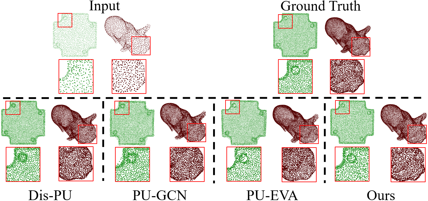
Figure 1: Most existing methods achieving satisfactory results for the input sparse point clouds with clear geometric structures (such as the hole on the green cover rear), but performing poorly for those with fuzzy geometric details (like the eyes of the red pig). Our results, with close proximity to the ground truth.

1 Introduction

Point clouds, as a most fundamental 3D representation, have been widely used in various downstream tasks such as 3D reconstruction [19, 25], autonomous driving [4, 16, 50], and robotics technology [44, 20]. However, raw point clouds captured from 3D sensors often exhibit sparsity, noise, and non-uniformity. This is substantiated across diverse publicly available benchmark datasets, such as KITTI [8], ScanNet [5]. Hence, point cloud upsampling, which involves the transformation of sparse, incomplete, and noisy point clouds into denser, complete, and artifact-free representations, has garnered considerable research interest.

Inspired by deep learning, the pioneering work of PU-Net [46] is the first to utilize deep neural networks to address this problem. This first divides the input point cloud into multiple patches and then extracts multi-scale features. Subsequently, these features are aggregated and fed into an upsampling module to approximate the dense point cloud coordinates. Building this approach, for more accurate results, many works [45, 17, 18, 22, 31] optimize neural networks by focusing on sparse point cloud feature extraction and upsampling module design.

However, while these methods have achieved improved results, predicting dense point cloud coordinates via sparse point cloud features is an indirect approximating approach. Typically, these methods first utilize an encoder to extract sparse point cloud features, and then use a carefully designed upsampling module to fit dense point cloud coordinates. This approach has three limitations. First, the non-dominance of features causes the generated results to be more inclined toward the input sparse point clouds, struggling to represent reasonable geometry details from the ground truth, as Fig 1 illustrated. Second, the additional upsampling module designs increase the workload for algorithm designers and often disrupt the intrinsic coordinate mappings in points [46, 45, 31]. Third, they mostly require the joint supervision of the CD loss and other losses, making them sensitive to noise [41, 13].

In this paper, we consider the point cloud upsampling task as a conditional generation problem. This first explores the incorporation of probability models for point cloud upsampling. We propose a novel point cloud upsampling network, called PUDM, which is formally based on a conditional DDPM. Unlike previous methods, PUDM models the gradient of data distribution from dense point clouds (i.e., the ground truth), directly utilizing the dominant features to fit the ground truth, and decoupling the dependency on CD loss. Moreover, the auto-regressive nature of DDPM enables PUDM to efficiently avoid the additional upsampling module design, ensuring intrinsic point-wise mapping relationships in point clouds.

Simultaneously, to improves the ability of perceiving point features, PUDM employs a dual mapping paradigm. This naturally establishes a dual mapping relationship: between the generated sparse point cloud and the sparse point cloud, and between the dense point cloud and the noise in PUDM. In this context, PUDM has the ability to learn complex geometric structures from the ground truth, generating uniform surfaces aligned with the ground truth, as Fig 1.

Furthermore, we found that DDPM only models fixed-scale point cloud objects during training. To overcome the issue, we consider parameterizing a rate factor to exploit the prior knowledge of the scale between sparse point clouds and dense point cloud. In this way, PUDM facilitates the production of high-fidelity arbitrary-scale point clouds during inference.

In additional, benefiting from the inherent denoising architecture and the non-dependency for CD loss, PUDM demonstrates a remarkable degree of robustness in noise experiments.

Our key contributions can be summarized as:

• We systematically analyze and recognize conditional DDPM as a favorable model for generating uniform point clouds at arbitrary scales in point cloud upsampling tasks.

• We propose a novel network with a dual mapping for point cloud upsampling, named PUDM, which is based on conditional DDPM.

• By exploiting the rate prior, PUDM exhibits the ability of generating high-fidelity point clouds across arbitrary scales during inference.

• Comprehensive experiments demonstrate the outstanding capability of PUDM in generating geometric details in public benchmarks of point cloud upsampling.

2 Related Works

Learnable Point Cloud Upsampling. The integration of deep learning with formidable data-driven and trainable attributes has markedly accelerated progress within the 3D field. Thanks to the powerful representation capabilities of deep neural networks, directly learning features from 3D data has become achievable, such as PointNet [29], PointNet++ [30], DGCNN [28], MinkowskiEngine [2], and KPConv [40]. PU-Net [46] stands as the pioneer in integrating deep neural networks into point cloud upsampling tasks. This first aggregates multi-scale features for each point through multiple MLPs, and then expands them into a point cloud upsampling set via a channel shuffle layer. Following this pattern, some methods have achieved more significant results, such as MPU [45], PU-GAN [17], Dis-PU [18], and PU-GCN [31]. PU-EVA [22] is the first to achieve the arbitrary point clouds upsampling rates via edge-vector based affine combinations in one-time training. Subsequently, PUGeo [33] and NePs [7] believe that sampling points within a 2D continuous space can generate higher-quality results. Furthermore, Grad-PU [9] transforms the point cloud upsampling problem into a coordinate approximation task, avoiding the upsampling module design.

Most methods predict the dense point cloud coordinates via sparse point cloud features, and extend the point set relying on an upsampling module. This causes them to struggle to learn complex geometry details from the ground truth. Moreover, they frequently exhibit a susceptibility to noise due to depending on CD loss during training. In this paper, we consider transforming the point cloud upsampling task into a point cloud generation problem, and first utilize conditional DDPM to address the aforementioned issues.

DDPM for Point Cloud Generation. Inspired by the success in image generation tasks [34, 35, 36], there has been greater attention on directly generating point clouds through DDPM. [23] represents the pioneering effort in applying DDPM to unconditional point cloud generation. Subsequently, [51] extends the application of DDPM to the point cloud completion task by training a point-voxel CNN [21]. However, the voxelization process introduces additional computational complexity. Furthermore, PDR [24] takes raw point clouds as input. But this requires training the two stages (coarse-to-fine) of diffusion models, resulting in a greater time overhead.

In this paper, we explore to the application of conditional DDPM to handle the point cloud upsampling task. Unlike the point cloud generation and completion task, point cloud upsampling exhibits the difference of the point cloud scale between training and inference. We overcome this issue by exploiting a rate prior during training. Meanwhile, our method based on a dual mapping paradigm enables the efficient learning of complex geometric details in a single-stage training.

3 Denoising Diffusion Probabilistic Model

3.1 Background for DDPM

The forward and reverse process. Given the dense point cloud $x$ sampled from a meaningful point distribution $P_{data}$, and an implicit variable $z$ sampled from a tractable noise distribution $P_{latent}$, DDPM establishes the transformation relationship between $x$ and $z$ through two Markov chains. This conducts an auto-regressive process: a forward process $q$ that gradually adds noise to $x$ until $x$ degrades to $z$, and a reverse process $p$ that slowly removes noise from $z$ until $z$ recovers to $x$. We constrain the transformation speed using a time step $t\sim\mathcal{U}(T)$ ($T=1000$ in this paper).

Training objective under specific conditions. Given a set of conditions $C=\{c_{i}|i=1..S\}$, the training objective of DDPM under specific conditions is (please refer to the supplementary materials for the detailed derivation):

$$\begin{split}L(\theta)=\mathbb{E}_{t\sim U(T),\epsilon\sim\mathcal{N}(0,I)}||\epsilon-\epsilon_{\theta}(\sqrt{1-\overline{\alpha}_{t}}\epsilon+\sqrt{\overline{\alpha}_{t}}x_{0},C,t)||^{2}\end{split}$$ (1)

The gradient of data distribution. Furthermore, we use a stochastic differential equation (SDE) to describe the process of DDPM [39]:

$$\begin{split}s_{\theta}(x_{t},t)=\nabla_{x}\log(x_{t})=-\frac{1}{\sqrt{1-\overline{\alpha}_{t}}}\epsilon_{\theta}(x_{t},t)\end{split}$$ (2)

The training objective of DDPM is essentially equivalent to computing the score (the gradient of data distribution), which differs only by a constant factor $-\frac{1}{\sqrt{1-\overline{\alpha}_{t}}}$.

3.2 Analysis of DDPM for PCU

We pioneer the exploration of the advantages and limitations of DDPM for PCU, hoping these insights encourage more researchers to introduce probability models into PCU.

DDPM is an effective model for PCU. As mentioned in Sec 3.1, the auto-regressive nature of DDPM allows it to directly learn geometry details of the ground truth using the dominant features, generating closer-to-truth, fine-grained results.

Simultaneously, the reverse process of DDPM in PCU is:

$$p_{\theta}(x_{0:T},c)=p(x_{T},c)\prod_{t=1}^{T}p_{\theta}(x_{t-1}|x_{t},c)$$ (3)

where $c$ means the sparse point cloud sampled from a data distribution $P_{c}$. According to Eq 3, the condition $c$ participates in each step of the reverse process. In fact, this is usually achieved using an additional branch network interacting with the noise network, without intrinsically disrupting the auto-regressive process of DDPM, thus cleverly avoiding to design an additional upsampling module. Moreover, the process naturally defines a one-to-one point-wise mapping relationship between the dense point cloud and the noise, preserving the order of points in the diffusion process.

Furthermore, the efficient denoising architecture and the decoupling of CD loss through the auto-regressive nature significantly support the strong noise robustness of DDPM.

The limitations of DDPM in PCU. While DDPM showcases some advantageous attributes within PCU, it also harbors certain potential limitations:

• Limitation 1: The lack of effective prior knowledge for point cloud conditional networks results in their weak feature perception capability [32, 48, 14], significantly affecting the final generation results (Tab 8). Although some methods [24] compensate for this problem via a two-stage (coarse-to-fine) training approach, they require a higher training cost.

• Limitation 2: The auto-regressive nature of DDPM provides robust modeling capabilities for fixed-scale objects during training, but it struggles to high-quality sample arbitrary-scale ones during inference (Tab 9). Some work treats multi-scale upsampling as multiple tasks [46, 45, 31], but it’s not advisable for DDPM due to the excessively high training cost.

4 Methodology

4.1 Dual mapping Formulation

For limitation 1, we adopt a dual mapping paradigm. We first provide a formal exposition of its conception, subsequently delineating the manner in which PUDM aligns with these principles, with a particular emphasis on its role.

Given two point sets of $X_{1}=\{x_{1}^{i}\in\mathbb{R}^{3}|i=1..M\}$, and $X_{2}=\{x_{2}^{i}\in\mathbb{R}^{3}|i=1..N\}$ from different data distributions, a network $f_{x}$ with a dual-branch ($\{f_{1},f_{2}\}=f_{x}$) structure, and the corresponding supervision signals for these branches ($\{l_{1},l_{2}\}=l_{x}$) , if $f_{x}$ satisfies:

$$Y_{1}=f_{1}(X_{1}),\quad Y_{2}=f_{2}(X_{2})$$ (4)

where $Y_{1}=\{y_{1}^{i}\in\mathbb{R}^{3}|i=1..M\}$, $Y_{2}=\{y_{2}^{i}\in\mathbb{R}^{3}|i=1..N\}$. $f_{x}$ can be claimed as a dual mapping network. Eq 5 means that each element in the original input has one and only one corresponding element in the final output in each branch. Similarly, we can further extend this concept to single mapping network ($\{f_{1}\}=f_{x},\{l_{1}\}=l_{x}$), and multiple mapping network ($\{f_{i}|i=1..n\}=f_{x},\{l_{i}|i=1..n\}=l_{x}$).

In PUDM, we only require the conditional network to meet the above condition, because the noise network inherently builds a one-to-one point-wise mapping between input and output [24]. Specifically, we first force the output $y_{c}=\{y_{c}^{i}\in\mathbb{R}^{3}|i=1..M\}$ from the conditional network $f_{\psi}$ to approximate the sparse point cloud $c=\{c^{i}\in\mathbb{R}^{3}|i=1..M\}$ coordinates via a MLP, and then optimize the process via the mean squared error loss:

$$L(\psi)=\mathbb{E}_{c\sim P_{c}}||c-f_{\psi}(c)||^{2}$$ (5)

Formally, this establishes a one-to-one point-wise mapping between the input and output for the conditional network, $y_{c}=f\psi(c)$.

For point cloud tasks with unordered structures, this pattern effectively enhances network capability in capturing point features by preserving the ordered relationships between input and output points [3, 12]. Moreover, corresponding supervision signals ensure adequate training for each branch network (Fig 7), providing an effective strategy to address the challenge of lacking robust 3D pre-trained models as substitutes for conditional branch networks in point cloud generation tasks.

4.2 Rate Modeling

For limitation 2, drawing inspiration from the practice of adding class labels in conditional probability models [27, 6, 10], we propose a simple and effective approach to achieve high-quality arbitrary-scale sampling during inference. Specifically, we first add a rate label $r$ to each sample pair, $(c,x)\rightarrow(c,x,r)$ (the supplementary materials provide ablation studies for different forms of the rate label $r$). Subsequently, we parameter the rate factor using an embedding layer. In this way, the reverse process of DDPM is:

$$p_{\theta}(x_{0:T},c,r)=p(x_{T},c,r)\prod_{t=1}^{T}p_{\theta}(x_{t-1}|x_{t},c,r)$$ (6)

Eq 6 demonstrates that this simply adds an additional condition to DDPM, the rate prior $r$, without increasing the number of samples. Unlike class labels, we found in experiments that this conditional prior we exploited can significantly improve the generation quality of unseen-scale point clouds. The reason is that generating unseen-scale and seen-category objects usually are easier compared to generating seen-scale and unseen-category ones for models.

4.3 Network Architecture

In this section, we introduce the overall framework of PUDM, consisting of three crucial components: the conditional network (C-Net), the noise network (N-Net), and the Transfer Module (TM). This process is remarkably illustrated in Fig 2. The parameter setting and implementation details are provided in the supplementary materials.

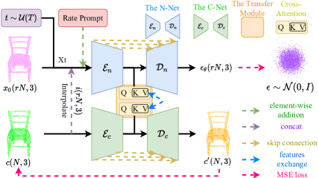
Figure 2: The overall framework of PUDM: The N-Net (upper branch) and the C-Net (lower branch) both establish a one-to-one point-wise mapping between input and output using mean squared error loss. They engage in information exchange through a transfer module (TM). Simultaneously, the rate prompt is provided to exploit the prior knowledge of the scale between sparse point clouds and dense point clouds.

The Conditional Network (C-Net). We use PointNet++ [30] as the backbone. This follows the standard U-Net framework. The encoder and decoder are composed of multiple Set Abstraction (SA) layers and Feature Propagation (FP) layers, respectively. Unlike PointNet++ using the max-pooling layer to filter features, we consider utilizing the self-attention layer to retain more fine-grained information [49, 26]. In addition, we only feed the sparse point cloud into the C-Net to ensure the feature extraction in a pure and effective manner.

The Noise Network (N-Net). The N-Net and the C-Net share the same network architecture. In contrast to the C-Net, we need to introduce additional guidance information to the N-Net for modeling the diffusion step.

We first transform the sparse point cloud $c\in\mathbb{R}^{N\times 3}$ into the interpolation point cloud $i\in\mathbb{R}^{rN\times 3}$ through the midpoint interpolation [9], and then concatenate $i$ and $x_{t}$ as the input for the N-Net. Meanwhile, we extract the global features from $i$ to enhance the semantic understanding. Furthermore, to identify the noise level, we encode the time step $t$. Finally, as mentioned in Sec. 4.2, we parameterized the rate factor $r$. These additional pieces of information are treated as global features, and incorporated into each stage of the encoder and the decoder in the N-Net.

The Transfer Module (TM). We propose a bidirectional interaction module (TM) to serve as an intermediary between the C-Net and the N-Net. We only place the TM at the bottleneck stage of U-Net, due to the significant computational efficiency and the abundant semantic information via the maximum receptive field [12, 15].

Given the outputs of the encoder in the C-Net and the N-Net, $F^{c}\in\mathbb{R}^{N_{e}^{c}\times C_{e}^{c}}$, $F^{n}\in\mathbb{R}^{N_{e}^{n}\times C_{e}^{n}}$ separately, the TM first transforms $F^{c}\rightarrow Q\in\mathbb{R}^{N_{e}^{c}\times C_{i}}$ and $F^{n}\rightarrow(K,V)\in\mathbb{R}^{N_{e}^{n}\times C_{i}}$ via MLPs. Next, we can obtain the fused feature:

$$F_{f}=MLP(softmax(\frac{QK^{T}}{\sqrt{C_{i}}})V)+F^{c}$$ (7)

Subsequently, $F_{f}$ is fed into a feed-forward network (FFN) to output the final features. Similarly, the same operation is also applied in reverse direction, so that information flows in both directions, $F^{c}\rightarrow F^{n}$ and $F^{n}\rightarrow F^{c}$.

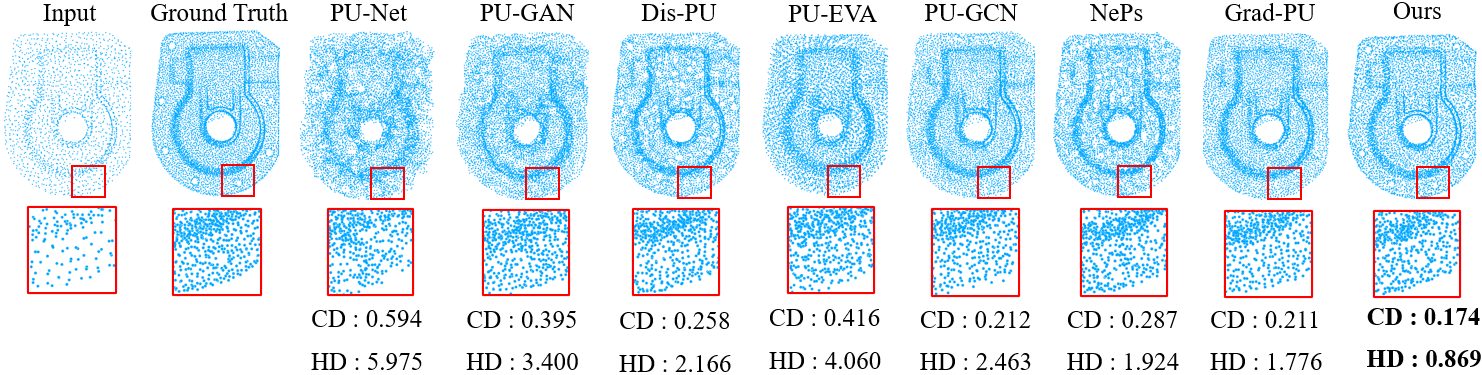
Figure 3: Visualization results at $4\times$ on PUGAN. Our result exhibits fewer outliers, and clearly captures geometric details from the ground truth (the holes on the casting).

4.4 Training and Inference

Training. As mentioned earlier (Sec. 4.1 and Sec. 4.2), PUDM is a dual mapping network, and models the rate prior during training. Therefore, the training objective is:

$$L_{mse}=L(\theta)+\alpha L(\psi)$$ (8)

where $\alpha$ means a weighting factor ($\alpha=1$ in this paper).

Inference. We found that adding the interpolated points $i$ as the guidance information significantly improves the generated quality during inference. Therefore, we iteratively transform $x_{t}$ into $x_{0}$ based on :

$$x_{t-1}=\gamma(\frac{1}{\sqrt{\alpha_{t}}}(x_{t}-\frac{1-a_{t}}{\sqrt{1-\overline{\alpha}_{t}}}\epsilon_{\theta}(x_{t},t,c,r))+\sigma_{t}\epsilon+i)$$ (9)

where $\gamma$ denotes a scale factor ($\gamma=0.5$ in this paper).

5 Experiments

5.1 Experiment Setup

Dataset. In our experiments, we utilize two public benchmarks (PUGAN [17], PU1K [31]) for evaluation. We adhere to the official training/testing partitioning protocols for these datasets. This uses Poisson disk sampling [47] to generate 24,000 and 69,000 uniform patches for training, respectively. Each patch contains 256 points, while the corresponding ground truth has 1024 points. Meanwhile, 27 and 127 point clouds are used for testing, respectively. The input sparse point clouds consist of 2048 points, and are upsampled to $2048\times R$ points via evaluated methods.

Metrics. Following [46, 45, 9], we employ the Chamfer Distance (CD $\times\;10^{-3}$), Hausdorff Distance (HD $\times\;10^{-3}$), and Point-to-Surface Distance (P2F $\times\;10^{-3}$) as evaluation metrics in our experiments.

5.2 Comparison with SOTA

Results on PUGAN. We first conduct the point cloud upsampling at low upsampling rate ($4\times$) and high upsampling rate ($16\times$) on PUGAN. Table 1 illustrates the substantial superiority of our method in geometric detail description compared to other methods, as evidenced by significantly reduced CD and HD. Because our method models the gradient of data distribution from dense point clouds, facilitating the direct approximation of geometric details from the ground truth, thereby yielding higher accuracy of our results. Fig 3 further substantiates our viewpoint, and shows that our method produces fewer outliers, aligning with more uniform surfaces, finer geometric details, and closer to the ground truth.

In addition, despite P2F falling slightly behind Grad-PU [9] at $4\times$, the difference is insignificant due to the asymmetry between points and surfaces [17, 9].

Methods	$4\times$				$16\times$
	CD$\downarrow$	HD$\downarrow$	P2F$\downarrow$		CD$\downarrow$	HD$\downarrow$	P2F$\downarrow$
PU-Net [46]	0.529	6.805	4.460		0.510	8.206	6.041
MPU [45]	0.292	6.672	2.822		0.219	7.054	3.085
PU-GAN [31]	0.282	5.577	2.016		0.207	6.963	2.556
Dis-PU [18]	0.274	3.696	1.943		0.167	4.923	2.261
PU-EVA [22]	0.277	3.971	2.524		0.185	5.273	2.972
PU-GCN [31]	0.268	3.201	2.489		0.161	4.283	2.632
NePS [7]	0.259	3.648	1.935		0.152	4.910	2.198
Grad-PU [9]	0.245	2.369	1.893		0.108	2.352	2.127
Ours	0.131	1.220	1.912		0.082	1.120	2.114

Table 1: The results of $4\times$ and $16\times$ on PUGAN. Our method significantly surpasses other methods in terms of CD and HD.

Arbitrary Upsampling Rates on PUGAN. Similarly to [9], we perform comparative analyses across various rates on PUGAN. Tab 2 shows that our method steadily outperforms Grad-PU [9] across nearly all metrics. In particular, our method demonstrates a significant performance advantage in terms of CD and HD, further affirming the superiority in learning complex geometric details.

Moreover, we visualize the results at higher upsampling rates ($16\times$, $32\times$, $64\times$, and $128\times$) in Fig 4. Our results obviously exhibit more complete, uniform, and smooth compared to Grad-PU [9].

Results on PU1K. Furthermore, we also conduct the evaluation at $4\times$ on more challenging PU1K [31]. As reported in Tab 3, our method continues to demonstrate substantial advantages in terms of CD and HD compared to other methods.

Rates	Grad-PU [9]				Ours
	CD$\downarrow$	HD$\downarrow$	P2F$\downarrow$		CD$\downarrow$	HD$\downarrow$	P2F$\downarrow$
$2\times$	0.540	3.177	1.775		0.247	1.410	1.812
$3\times$	0.353	2.608	1.654		0.171	1.292	1.785
$5\times$	0.234	2.549	1.836		0.116	1.244	1.794
$6\times$	0.225	2.526	1.981		0.107	1.235	1.980
$7\times$	0.219	2.634	1.940		0.106	1.231	1.952

Table 2: Grad-PU $vs.$ ours at various rates on PUGAN. Benefiting from the rate modeling, our method still exhibits remarkable performance at various rates.

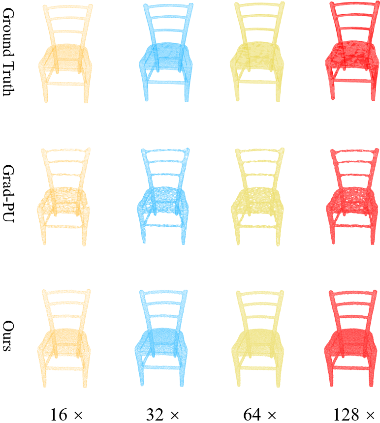
Figure 4: Grad-PU $vs.$ ours at large rates on PUGAN. Our method consistently generates more uniform and smooth surfaces (these results are achieved using an NVIDIA 3090 GPU).

Methods	CD$\downarrow$	HD$\downarrow$	P2F$\downarrow$
PU-Net [46]	1.155	15.170	4.834
MPU [45]	0.935	13.327	3.511
PU-GCN [31]	0.585	7.577	2.499
Grad-PU [9]	0.404	3.732	1.474
Ours	0.217	2.164	1.477

Table 3: The results of $4\times$ on PU1K. We utilize the experimental results from the original paper.Our method outperforms other methods across nearly all metrics.

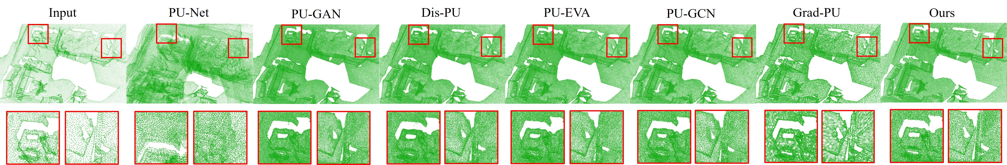
Figure 6: The results of $4\times$ on ScanNet. Our results exhibit reduced instances of outliers, concurrently generating more uniform and complete surfaces.

Result on Real datasets. Additionally, we conduct the evaluation on real indoor (ScanNet [5]) and outdoor (KITTI [8]) scene datasets. All methods are only trained on PUGAN. Upsampling scene-level point clouds poses greater challenges than upsampling object-level ones, due to the former having more intricate geometric structures. Due to the absence of the ground truth, our analysis is confined to qualitative comparisons. In Fig 5, our method still generates reasonable and smooth surfaces on some complex structures, while other methods exhibit artifacts such as overlap and voids. Simultaneously, Fig 6 illustrates that our results show more complete and fewer outliers. Although Grad-PU [9] also demonstrates good outlier results, it generates a considerable amount of uneven surfaces.

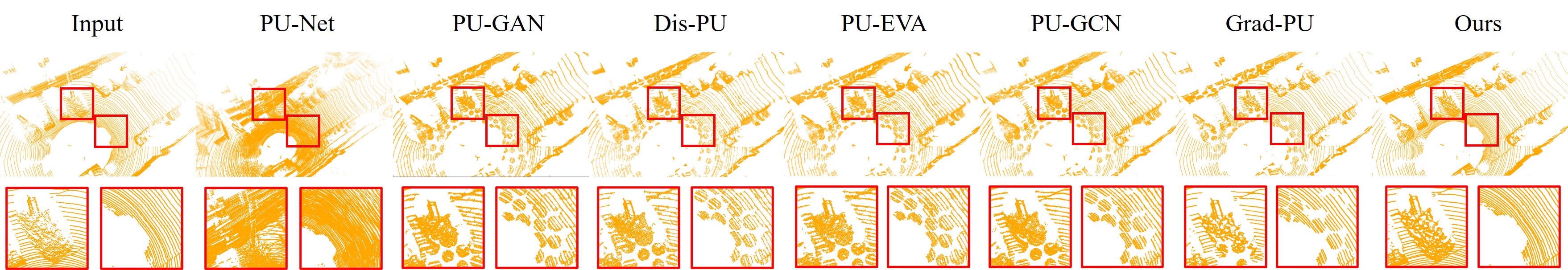
Figure 5: The results of $4\times$ on KITTI. Our method noticeably generates more reasonable and uniform results on some complex geometric structures.

5.3 Validation for Noise Robustness

Gaussian Noise. To demonstrate the robustness, we perturb the sparse point clouds with Gaussian noise sampled $\mathcal{N}(0,I)$ added at different noise levels $\tau$.

As shown in Tab 4, our method significantly outperforms other methods under multiple level noise perturbations ($\tau=0.01$, $\tau=0.02$). Specifically, this is because our method models the noise $\epsilon$ (the gradient of data distribution) and avoids CD loss during training.

Noise Levels	$\tau=0.01$				$\tau=0.02$
Methods	CD$\downarrow$	HD$\downarrow$	P2F$\downarrow$		CD$\downarrow$	HD$\downarrow$	P2F$\downarrow$
PU-Net [46]	0.628	8.068	9.816		1.078	10.867	16.401
MPU [45]	0.506	6.978	9.059		0.929	10.820	15.621
PU-GAN [31]	0.464	6.070	7.498		0.887	10.602	15.088
Dis-PU [18]	0.419	5.413	6.723		0.818	9.345	14.376
PU-EVA [22]	0.459	5.377	7.189		0.839	9.325	14.652
PU-GCN [31]	0.448	5.586	6.989		0.816	8.604	13.798
NePS [7]	0.425	5.438	6.546		0.798	9.102	12.088
Grad-PU [9]	0.414	4.145	6.400		0.766	7.336	11.534
Ours	0.210	2.430	6.070		0.529	5.471	9.742

Table 4: The results of $4\times$ at low-level Gaussian noise on PUGAN. Our method significantly outperforms other methods in terms of noise robustness.

Moreover, we also conduct the evaluation under more challenging noise perturbations. Tab 5 shows that our method exhibits stronger robustness results at higher level noise perturbations ($\tau=0.05$ and $\tau=0.1$). This indicates that our method exhibits a trend of resilience for the noise robustness.

Noise Levels	$\tau=0.05$				$\tau=0.1$
Methods	CD$\downarrow$	HD$\downarrow$	P2F$\downarrow$		CD$\downarrow$	HD$\downarrow$	P2F$\downarrow$
PU-Net [46]	1.370	13.729	23.249		1.498	14.193	23.846
MPU [45]	1.247	11.645	22.189		1.321	12.415	23.841
PU-GAN [31]	1.124	9.091	21.252		1.271	10.911	23.174
Dis-PU [18]	1.076	7.921	20.603		1.244	10.913	22.845
PU-EVA [22]	1.057	7.910	20.044		1.226	9.305	22.296
PU-GCN [31]	1.263	9.869	22.835		1.456	11.063	25.213
NePS [7]	1.143	9.645	18.642		1.198	9.874	20.162
Grad-PU [9]	0.978	8.057	16.927		1.118	8.946	18.845
Ours	0.618	5.386	14.751		0.853	6.239	16.845

Table 5: The results of $4\times$ at high-level Gaussian noise on PUGAN. Compared to other methods, our method demonstrates a more favorable upward trend for robustness to noise.

Random Noise. Furthermore, we also investigated the performance of our method on other noise distribution. Admittedly, while our method still keeps SOTA performance, as shown in Tab 6, the results on random noise show significantly lower than that on Gaussian noise.

We provide an intuitive explanation. Eq 2 demonstrates that the training objective of DDPM is to fit the gradient of data distribution (modeling the noise $\epsilon$, named score) [39]. Essentially, DDPM learns the direction of noise generation. When the conditions with noise are considered, the disturbance in the direction exhibits relatively small, because the noise has a similar distribution to $\epsilon$. Therefore, during inference, our method demonstrates robustness to similar noise distributions of $\epsilon$ (Gaussian noise), but performs poorly when faced with different ones.

Noise Levels	$\tau=0.05$				$\tau=0.1$
Methods	CD$\downarrow$	HD$\downarrow$	P2F$\downarrow$		CD$\downarrow$	HD$\downarrow$	P2F$\downarrow$
PU-Net [46]	1.490	14.473	23.223		1.725	15.442	25.251
MPU [45]	1.224	10.842	20.456		1.545	11.645	23.512
PU-GAN [31]	1.034	7.757	18.617		1.327	9.700	21.321
Dis-PU [18]	1.006	6.856	17.873		1.314	7.463	20.980
PU-EVA [22]	1.024	7.534	18.179		1.334	8.056	21.158
PU-GCN [31]	1.045	9.643	18.899		1.325	10.877	21.633
NePS [7]	1.048	7.345	18.054		1.321	9.645	21.314
Grad-PU [9]	1.067	6.634	17.734		1.399	7.215	21.028
Ours	0.998	6.110	17.558		1.310	6.732	20.564

Table 6: The results of $4\times$ at high-level random noise on PUGAN. Our method consistently outperforms other methods on all metrics.

5.4 Effectiveness in Downstream Task

We evaluate the effectiveness of upsampling quality in the downstream task: point cloud classification. Meanwhile, we also conducted experiments on point cloud part segmentation, please refer to the supplementary materials.

PointNet [29] and PointNet++ [30] are chosen as the downstream task models due to their significant performance and widespread influence in 3D tasks. We follow the official training and testing procedures. Simultaneously, we select ModelNet40 [42] (40 categories) and ShapeNet [1] (16 categories) as the benchmarks for point cloud classification. For a fairer and more effective evaluation, we use only 3D coordinates as the input. Similar to the evaluated strategy on real datasets, all point cloud upsampling methods are only trained on PUGAN.

For evaluation, we first subsample 256/512 points from test point clouds on ModelNet40/ShapeNet. Subsequently, they are upsampled to 1024/2048 points through evaluation methods. As depicted in Tab 7, our results significantly improve the classification accuracy compared to the low-res point clouds, and consistently outperforms other methods across all metrics.

Datasets	ModelNet40 ($\%$)				ShapeNet ($\%$)
Models	PointNet		PointNet++		PointNet		PointNet++
Methods	IA$\uparrow$	CA$\uparrow$	IA$\uparrow$	CA$\uparrow$	IA$\uparrow$	CA$\uparrow$	IA$\uparrow$	CA$\uparrow$
Low-res	87.15	83.12	88.87	84.45	97.61	95.09	98.20	96.11
High-res	90.74	87.14	92.24	89.91	98.89	96.61	99.27	98.18
PU-Net [46]	88.72	85.25	88.99	85.43	97.99	95.69	98.57	96.35
MPU [45]	89.04	85.84	89.54	86.51	98.03	95.92	98.94	96.81
PU-GAN [31]	89.95	85.68	90.45	87.23	98.75	95.70	90.45	87.23
Dis-PU [18]	88.70	85.34	89.56	86.53	98.80	96.07	99.00	97.15
PU-EVA [22]	89.27	85.63	89.96	86.86	98.72	95.69	99.07	97.58
PU-GCN [31]	89.77	85.38	89.45	86.15	98.78	96.06	99.03	97.42
NePS [7]	90.01	86.15	90.32	87.34	98.94	96.20	99.12	97.94
Grad-PU [9]	90.05	86.06	89.98	87.49	98.82	96.19	99.10	97.63
Ours	90.33	86.54	92.14	89.42	98.85	96.58	99.13	97.99

Table 7: The results of point cloud classification. ”Low-res” refers to the point cloud subsampled, while ”High-res” denotes the original test point cloud. Meanwhile, ”IA” stands for instance accuracy, and ”CA” denotes class accuracy. Our results have more reasonable, finer-grained, and closer-to-ground truth geometric structures, thereby achieving more significant classification accuracy.

5.5 Ablation Study

With/Without the dual mapping paradigm. Thanks to the rich and structured data, the conditional networks for text or images can be replaced by powerful pre-trained models [35, 43, 36, 37]. However, robust pre-trained backbones are lacking in the 3D field due to sparse data and challenging feature extraction [32, 48, 14]. In this paper, we employ the dual mapping paradigm to augment the capability of perceiving point features within PUDM, ensuring the comprehensive training of the C-Net. To validate this point, we remove the supervision signal from the C-Net to disrupt this pattern. Meanwhile, we also validate the importance of the C-Net by retaining only the N-Net in PUDM .

As reported in Tab 8, disrupting the dual mapping pattern leads to a significant decrease in performance due to the weakened point feature perception ability of the C-Net. Fig 7 visualizes the results of the C-Net generating input sparse points using the dual mapping paradigm.

Meanwhile, although removing the C-Net can maintain a single mapping pattern, as demonstrated in prior research [46, 31, 22], sparse point cloud feature extraction plays a pivotal role in PCU.

Methods	CD$\downarrow$	HD$\downarrow$	P2F$\downarrow$
Without the C-Net	0.212	2.015	2.284
Without the dual mapping	0.168	1.498	2.013
With the dual mapping	0.131	1.220	1.912

Table 8: Ablation study of the dual mapping paradigm. The construction of the dual mapping pattern evidently achieves the best performance.

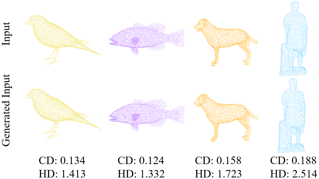
Figure 7: Visualization results of the C-Net generating sparse point clouds on PUGAN. This demonstrates that the C-Net has been effectively trained.

With/Without the rate prior. As mentioned in Sec 4.2, we introduce the rate prior into PUDM during training to achieve high-quality generation of point clouds during inference. Tab 9 demonstrates the effectiveness of this approach. Without the rate prior, the overall performance notably decreases, and exhibits significant fluctuations (performing better at $4\times$, but worse at other rates).

Rates	Without the rate modeling				With the rate modeling
	CD$\downarrow$	HD$\downarrow$	P2F$\downarrow$		CD$\downarrow$	HD$\downarrow$	P2F$\downarrow$
$2\times$	0.295	1.816	2.014		0.247	1.410	1.812
$3\times$	0.224	1.544	1.975		0.171	1.292	1.785
$4\times$	0.158	1.512	1.815		0.131	1.220	1.912
$5\times$	0.166	1.548	1.944		0.116	1.244	1.794
$6\times$	0.151	1.528	1.956		0.107	1.235	1.980
$7\times$	0.144	1.425	1.988		0.106	1.231	1.952
$8\times$	0.139	1.399	1.921		0.104	1.215	1.875

Table 9: Ablation study of the rate prior. Utilizing the rate prior significantly enhances the quality of arbitrary-scale sampling.

Single/Multiple Transfer Module. In this paper, we employ a TM positioned at the bottleneck stage of the U-Net, as its maximum receptive field provides ample contextual information [12, 15]. Meanwhile, we also attempt to place multiple TMs at each stage in U-Net to enable the interaction of multi-scale information [24]. Tab 10 shows that although multiple TMs lead to a slight improvement in terms of CD loss, it is not cost-effective due to the significant increase in computational cost.

Methods	CD$\downarrow$	HD$\downarrow$	P2F$\downarrow$	Params$\downarrow$
Multiple TMs	0.129	1.235	1.953	28.65M
Single TM	0.131	1.220	1.912	16.03M

Table 10: Ablation study of the Transfer Module. Using the single TM clearly strikes a balance between performance and computational cost.

6 Conclution

In this paper, we systematically analyze and identify the potential of DDPM as a promising model for PCU. Meanwhile, we propose PUDM based on conditional DDPM. PUDM enables to directly utilize the dominant features to generate geometric details approximating the ground truth. Additionally, we analyze the limitations of applying DDPM to PCU (the absence of efficient prior knowledge for the conditional network and the fixed-scale object modeling), and propose corresponding solutions (a dual mapping paradigm and the rate modeling). Moreover, we offer a straightforward explanation regarding the robustness to noise for PUDM observed in experiments.

1 Additional Ablation Study

We provide additional ablation studies to deepen the analysis and understanding for our method.

Rate label form. Our method achieves high-quality arbitrary-rate sampling during inference by parameterizing a rate factor. Therefore, we explore the impact of different rate label forms for the model performance. We provide additional information regarding the scale of points, such as the number of points. As shown in Tab 1, the performance difference for the model is relatively small (the variation $<0.02$ for CD). This reason is that the rate label is solely modeled to identify the scale difference between the sparse point cloud and the dense point cloud, thus it can not significantly improve the performance of the model.

Rate Label Forms	CD$\downarrow$	HD$\downarrow$	P2F$\downarrow$
[256,1024,3]	0.143	1.258	1.907
[256,1024]	0.145	1.352	1.913
[0.256,1.024]	0.141	1.289	1.954
[3,]	0.131	1.220	1.912

Table 1: The ablation study of the rate label form at $4\times$ on PUGAN [17]. Our method performs optimally, when $r=[3,]$ (we set $r=[0,]$ to represent $1\times$).

Sampling intervals. Our method is formally based on conditional DDPM, thus inevitably lagging behind existing non-DDPM-based methods in terms of sampling speed. Therefore, we conduct the ablation study between the quality and time of generating point clouds under different sampling intervals. To stay within the framework of DDPM, we refraine from applying acceleration methods such as DDIM [38]. This only changes the sampling interval during inference, without retraining the model.

Tab 2 shows the trade-off between the performance and the generating time of our method under different sampling intervals. Surprisingly, although the overall performance of the model decreases with increasing sampling intervals, this does not follow a linear trend, presenting an irregular state. We believe that the performance variation of the model is not only related to the sampling interval but also to the distance from $x_{1}$ to $x_{0}$. When the distance of time step between $x_{1}$ and $x_{0}$ is smaller, the model performs better, such as the sampling interval $=12$ (with a distance of 3 time steps between $x_{1}$ and $x_{0}$). In other words, when given some close time intervals, we should choose the sampling interval that brings $x_{1}$ closest to $x_{0}$, rather than the one that evenly divides the total time steps.

Intervals	Distance	CD$\downarrow$	HD$\downarrow$	P2F$\downarrow$	Times(s)$\downarrow$
50	49	0.320	2.738	3.145	0.410
40	39	0.303	2.608	3.124	0.473
30	9	0.221	2.234	2.054	0.584
20	19	0.248	2.380	2.064	0.784
12	3	0.202	1.976	1.984	1.302
10	9	0.210	2.001	2.087	1.392
1	1	0.131	1.220	1.934	14.773

Table 2: Ablation study of different sampling interval at $4\times$ on PUGAN [17]. “Distance” means the distance of time steps between $x_{1}$ and $x_{0}$. When the sampling interval $=12$, the performance and sampling speed of our methods keep a favorable balance. Meanwhile, we showcase the visual results for the sampling interval $=12$ and $=30$ in Fig 5.

2 Additional Comparative Experiments

Sampling speed. We conduct the evaluation of sampling speed. Admittedly, as shown in Tab 3, our method lags behind in terms of time compared to existing methods. However, a positive aspect is: due to the remarkably strong performance, our method still can maintain state-of-the-art performance even with a certain loss of precision, while also exhibiting a comparable sampling speed (when we set sampling interval $=30$).

	PU-Net [46]	MPU [45]	PU-GAN [31]	Dis-PU [18]	PU-EVA [22]
Average	0.446	0.487	0.618	0.724	0.587
Times(s)$\downarrow$	PU-GCN [31]	NePS [7]	Grad-PU [9]	Ours	I=30
	0.531	0.479	0.403	14.773	0.584

Table 3: The results of sampling speed at $4\times$ on PUGAN [17]. ’I=30’ means that the sampling interval is set to 30 during inference for our method. Our method still maintains the state-of-the-art performance at the comparable sampling speed (For the specific performance, please refer to the table 1 in the main paper).

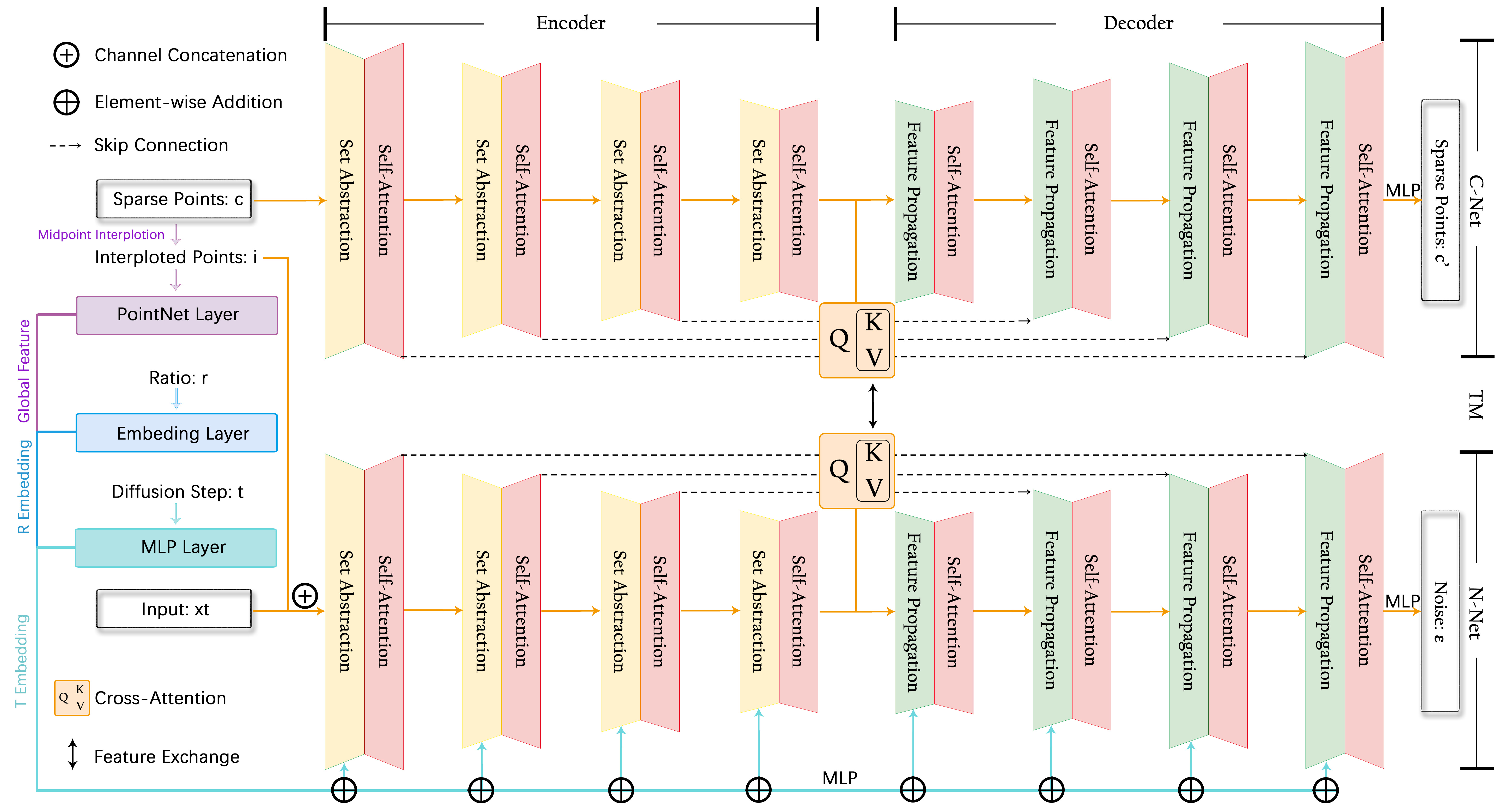
Figure 1: The network detail of PUDM. The encoder of the N-Net and the C-Net consists of set abstraction (SA) layers and self-attention layers. Simultaneously, the decoder consists of feature propagation (FP) layers and self-attention layers. The transfer module used for interaction between the N-Net and the C-Net consists of two cross-attention modules. Compared to the C-Net, the N-Net requires additional information for modeling the diffusion step: the global features, the $R$ embedding, and the $T$ embedding.

Point Cloud Part Segmentation. We evaluate the quality of point cloud upsampling on point cloud part segmentation. Tab 4 displays extremely poor results for all point cloud upsampling methods (class accuracy $<40\%$).

Existing point cloud upsampling methods (including our methods) are not proficient in semantic-related downstream tasks such as point cloud segmentation and point cloud detection. This is because the semantic order of points is disrupted during the point cloud upsampling process, making each point struggle to align with the semantic label. This greatly limits the application scope of point cloud upsampling in downstream tasks.

In fact, because the semantic label is uniquely mapped to each point in point clouds, their distributions are inherently similar. Therefore, the model may be able to maintain the semantic order of points during upsampling point clouds.

Datasets	PointNet [29] ($\%$)				PointNet++ [30] ($\%$)
Methods	IA$\uparrow$	CA$\uparrow$	Im$\uparrow$	Cm$\uparrow$	IA$\uparrow$	CA$\uparrow$	Im$\uparrow$	Cm$\uparrow$
Low-res	92.16	81.12	77.13	81.11	92.97	84.99	81.10	83.13
High-res	93.47	83.05	79.01	83.99	94.34	86.27	82.91	85.61
PU-Net [46]	51.92	36.05	32.69	35.79	52.04	36.25	32.66	35.90
MPU [45]	52.01	36.16	32.76	35.89	52.14	36.28	32.71	36.04
PU-GAN [31]	52.01	35.94	32.78	35.90	52.25	36.08	32.73	36.10
Dis-PU [18]	52.38	36.02	32.79	35.96	52.71	36.16	32.78	36.16
PU-EVA [22]	51.80	35.94	32.69	35.82	52.04	36.13	32.65	35.94
PU-GCN [31]	51.67	35.87	32.58	35.58	51.89	36.03	32.65	35.79
NePS [7]	51.71	35.91	32.63	35.61	52.01	36.11	32.67	35.87
Grad-PU [9]	52.22	36.02	32.75	36.07	52.46	35.29	32.97	36.31
Ours	51.88	36.08	32.67	36.00	52.11	36.48	32.99	36.34

Table 4: The results of point cloud part segmentation on ShapeNet [1]. ”Low-res” refers to the point cloud subsampled with 512 points, while ”High-res” denotes the original test point cloud with 2048 points. Meanwhile, ”IA” stands for instance accuracy, and ”CA” denotes class accuracy. ”Im” means instance mIoU, and ”Cm” denotes class mIoU. All methods yield very poor results, as existing point cloud upsampling methods struggle to maintain the semantic order of points.

3 Implementation

The network detail of PUDM is shown in Fig 1. We employ the same training configuration for PUGAN and PU1K. Specifically, we configure batch size $=28$, and conduct $1000$ epochs using an NVIDIA 3090 GPU, taking approximately $5$ days for PUGAN. For the C-Net and the N-Net, the sampling points/the channel dimensions are (1024, 256, 64, 16)/(64, 128, 256, 512) and (1024, 256, 64, 16)/(128, 256, 256, 512), respectively. Meanwhile, in the TM, we set the number $=4$ of head to improve the modeling capacity of our model, and the latent dimension $=64$. In addition, the global features with a dimension of $1024$ are extracted from the interpolated point cloud $i$ through a two-stage PointNet [29]. The parameters of the $R$ embedding layer are $(256,128)$, indicating that our method can upsample a point cloud to a maximum of 256 times. The time step $t$ is embedded dimension $=512$ via MLPs [11].

Encoder. In the Encoder, the SA first uses iterative farthest point sampling (FPS) to subsample the input points $p_{e}^{l}\in\mathbb{R}^{N^{l}\times 3}$ and the feature $f_{e}^{l}\in\mathbb{R}^{N^{l}\times C_{e}^{l}}$ into $p_{e}^{l}\in\mathbb{R}^{N^{l+1}\times 3}$ and $f_{e}^{l}\in\mathbb{R}^{N^{l+1}\times C_{e}^{l}}$ at level $l+1$ ($N^{l}>N^{l+1}$). Subsequently, we locate $K$ nearest neighbors in $p_{e}^{l}$, and aggregate the feature $f_{e}^{l}$ and neighbors into $g_{in}\in\mathbb{R}^{N^{l+1}\times C_{e}^{l}\times K}$. Next, we further extract the neighborhood features by transforming $g_{in}$ into $g_{out}\in\mathbb{R}^{N^{l+1}\times C_{e}^{l+1}\times K}$ through MLPs. Simultaneously, to preserve more details, we use the residual connection to aggregate $MLP(g_{in})$ and $g_{out}$. Finally, unlike PointNet++ [30] using the max-pooling layer to filter features, we consider using the self-attention layer to retain more fine-grained information [49, 26], $f_{e}^{l+1}\in\mathbb{R}^{N^{l+1}\times C_{e}^{l+1}}$.

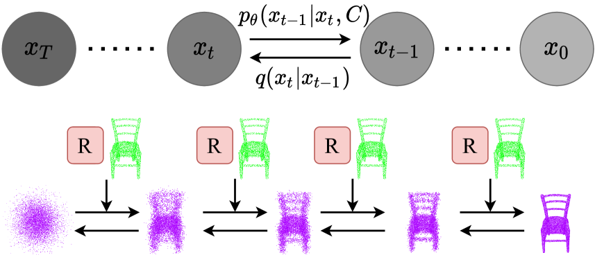
Figure 2: Visualization of the forward process and the reverse process of PUDM. For the forward process, the dense point cloud $x_{0}$ is gradually added noise according to $q(x_{t}|x_{t-1})$, until $x_{0}$ degrades to $x_{T}$. Simultaneously, for the reverse process, $x_{T}$ is slowly removed noise according to $p_{\theta}(x_{t-1}|x_{t},C)$, until $x_{T}$ recovers to $x_{0}$. We consider adding the conditions at each time step in the reverse process, the sparse point cloud $c$ and the rate prompt $R$, to control the generation of the dense point cloud.

Decoder. In the Decoder, the FP is similar to the SA, while the FP transforms the input feature $f_{d}^{l}\in\mathbb{R}^{N^{l}\times C_{d}^{l}}$ into $f_{d}^{l}\in\mathbb{R}^{N^{l+1}\times C_{d}^{l}\times K}$ through upsampling ($N_{l}<N_{l+1}$). Subsequently, we feed $f_{d}^{l}$ into a self-attention layer to obtain $f_{d}^{l}\in\mathbb{R}^{N^{l+1}\times C_{d}^{l}}$. Simultaneously, to propagate features, we aggregate $f_{d}^{l}$ with the points $p_{d}^{l}$ and the features $f_{e}^{l}$ from the SA at the same level. Finally, we transform $f_{d}^{l}$ into $f_{d}^{l+1}\in\mathbb{R}^{N^{l+1}\times C_{d}^{l+1}}$ through MLPs.

4 Formula Derivation of DDPM for PCU

In this section, we provide the theoretical foundation for the application of DDPM in PCU. Due to the page limitations, our derivation process focuses more on the overall logic, overlooking some details.

The forward process. The forward process $q$ is modeled as a Markov chain, while the each step follows an independent Gaussian distribution. This gradually adds noise to $x$ until $x$ degrades to $z$. The process is irrelevant of the condition $c$ (i.e. the sparse point cloud). Formally, given a time step $t\sim\mathcal{U}(T)$ and the dense point cloud $x_{0}\sim P_{data}$, we can compute the forward process by the conditional distribution $q(x_{1:T}|x_{0})$:

$$\begin{split}q(x_{1:T}|x_{0})=\frac{q(x_{0:T})}{q(x_{0})}\quad\quad\quad\quad\quad\quad\quad\quad\quad\quad\quad\quad\quad\quad\;\;\\ =\frac{{\color[rgb]{1,0,0}q(x_{T}|x_{0:T-1})}q(x_{0:T-1})}{q(x_{0})}\quad\quad\quad\quad\quad\quad\quad\quad\\ {\color[rgb]{0,0,1}Markov\;Property:}\quad\quad\quad\quad\quad\quad\quad\quad\quad\quad\quad\quad\quad\quad\quad\\ =\frac{{\color[rgb]{1,0,0}q(x_{T}|x_{T-1})}q(x_{T-1}|x_{0:T-2})q(x_{0:T-2})}{q(x_{0})}\quad\quad\\ =\frac{q(x_{T}|x_{T-1})q(x_{T-1}|x_{T-2})...q(x_{1}|x_{0}){\color[rgb]{1,0,0}\cancel{q(x_{0})}}}{{{\color[rgb]{1,0,0}\cancel{q(x_{0})}}}}\\ =\prod_{t=1}^{T}q(x_{t}|x_{t-1})\quad\quad\quad\quad\quad\quad\quad\quad\quad\quad\quad\quad\end{split}$$ (1)

where $q(x_{t}|x_{t-1})=\mathcal{N}(x_{t};\sqrt{1-\beta_{t}}x_{t-1},\beta_{t}I)$. $\beta_{t}$ is a predefined and increasing variance term ($\beta_{t}\in[0.0001,0.02]$ in this paper).

Meanwhile, to enable the sampling-differentiable training, we utilize the reparameterization trick[11] : $x_{t}=\mu+\sigma\epsilon_{t}$, $\epsilon_{t}\sim\mathcal{N}(\epsilon_{t};0,I)$. Next, we can obtain a more simplified formulation of computing $x_{t}$ by setting $\alpha_{t}=1-\beta_{t}$, and $\overline{\alpha}_{t}=\prod_{t=1}^{T}\alpha_{t}$:

$$\begin{split}x_{t}=\sqrt{1-\beta_{t}}x_{t-1}+\beta_{t}\epsilon_{t}\quad\quad\quad\quad\quad\quad\quad\quad\quad\quad\quad\quad\;\\ =\sqrt{\alpha_{t}}x_{t-1}+\sqrt{1-\alpha_{t}}\epsilon_{t}\quad\quad\quad\quad\quad\quad\quad\quad\quad\quad\;\;\;\;\;\\ =\sqrt{\alpha_{t}}(\sqrt{\alpha_{t-1}}x_{t-2}+\sqrt{1-\alpha_{t-1}}\epsilon_{t-1})+\sqrt{1-\alpha_{t}}\epsilon_{t}\\ =\sqrt{\alpha_{t}\alpha_{t-1}}x_{t-2}+{\color[rgb]{1,0,0}\sqrt{\alpha_{t}-\alpha_{t}\alpha_{t-1}}\epsilon_{t-1}+\sqrt{1-\alpha_{t}}\epsilon_{t}}\\ =\sqrt{\alpha_{t}\alpha_{t-1}}x_{t-2}+{\color[rgb]{1,0,0}\sqrt{1-\alpha_{t}\alpha_{t-1}}\epsilon}\quad\quad\quad\quad\quad\quad\quad\;\;\\ ...\quad\quad\quad\quad\quad\quad\quad\quad\quad\quad\quad\quad\quad\quad\quad\quad\quad\quad\quad\quad\quad\\ =\sqrt{\overline{\alpha}_{t}}x_{0}+\sqrt{1-\overline{\alpha}_{t}}\epsilon\quad\quad\quad\quad\quad\quad\quad\quad\quad\quad\quad\;\;\quad\end{split}$$ (2)

where $\epsilon$ represents the combination of multiple Gaussian noise terms.

Therefore, $x_{t}$ is only related to the dense point cloud $x_{0}$ and the time step $t$ in the forward process.

The reverse process. Similarly, the reverse process $p$ is also modeled as a Markov chain, while the each step is assumed to follow an independent Gaussian distribution. This slowly removes noise from $z$ until $z$ recovers to $x$. Formally, given a set of conditions $C=\{c_{i}|i=1..S\}$ (”$S$” means the number of conditions), we can compute the reverse process by the joint distribution $p_{\theta}(x_{0:T},C)$:

$$\begin{split}p_{\theta}(x_{0:T},C)={\color[rgb]{1,0,0}p_{\theta}(x_{0}|x_{1:T},C)}p_{\theta}(x_{1:T},C)\quad\quad\quad\quad\quad\quad\;\;\\ {\color[rgb]{0,0,1}Markov\;Property:}\quad\quad\quad\quad\quad\quad\quad\quad\quad\quad\quad\quad\quad\quad\quad\\ ={\color[rgb]{1,0,0}p_{\theta}(x_{0}|x_{1},C)}p_{\theta}(x_{1}|x_{2:T},C)p_{\theta}(x_{2:T},C)\quad\quad\quad\\ \quad\quad=p_{\theta}(x_{0}|x_{1},C)...p_{\theta}(x_{T}|x_{T-1},C)p(x_{T},C)\quad\;\;\;\;\;\;\\ =p(x_{T},C)\prod_{t=1}^{T}p_{\theta}(x_{t-1}|x_{t},C)\quad\quad\quad\quad\quad\quad\quad\;\;\\ {\color[rgb]{0,0,1}x_{T}\sim\mathcal{N}(x_{T};0,I)}\quad\quad\quad\quad\quad\quad\quad\quad\quad\quad\quad\quad\quad\quad\quad\quad\\ =p(x_{T})\prod_{t=1}^{T}p_{\theta}(x_{t-1}|x_{t},C)\quad\quad\quad\quad\quad\quad\quad\quad\;\;\\ \end{split}$$ (3)

When $C=\emptyset$, Eq 3 transforms into the reverse process of standard DDPM (i.e. unconditional DDPM).

Then, as DDPM is modeled to be reversible, we can directly compute the posterior distribution $q(x_{t-1}|x_{t},x_{0})$ in the forward process:

$$\begin{split}q(x_{t}|x_{t-1},x_{0})=\frac{{\color[rgb]{1,0,0}q(x_{t-1}|x_{t},x_{0})}q(x_{t},x_{0})}{q(x_{t-1},x_{0})}\quad\quad\quad\\ {\color[rgb]{1,0,0}q(x_{t-1}|x_{t},x_{0})}=\frac{q(x_{t}|x_{t-1},x_{0})q(x_{t-1}|x_{0})}{q(x_{t}|x_{0})}\quad\quad\\ {\color[rgb]{0,0,1}Markov\;Property:}\quad\quad\quad\quad\quad\quad\quad\quad\quad\quad\quad\quad\quad\quad\quad\\ =\frac{{\color[rgb]{1,0,0}q(x_{t}|x_{t-1})}q(x_{t-1}|x_{0})}{q(x_{t}|x_{0})}\quad\quad\;\;\;\;\;\end{split}$$ (4)

where $q(x_{t}|x_{t-1})=\mathcal{N}(x_{t};\sqrt{\alpha_{t}}x_{t-1},(1-\alpha_{t})I)$, $q(x_{t-1}|x_{0})=\mathcal{N}(x_{t-1};\sqrt{\overline{\alpha}_{t-1}}x_{0},(1-\overline{\alpha}_{t-1})I)$, and $q(x_{t}|x_{0})=\mathcal{N}(x_{t};\sqrt{\overline{\alpha}_{t}}x_{0},(1-\overline{\alpha}_{t})I)$. In fact, each time step in the reverse process aims to gradually fit the posterior distribution under corresponding time step in the forward process (the posterior distribution represents the inverse process of the forward process, not the reverse process of DDPM), i.e. $p_{\theta}(x_{t-1}|x_{t},C)\approx q(x_{t-1}|x_{t},x_{0})$. Therefore, deriving $p_{\theta}(x_{t-1}|x_{t},C)$ is equated to deriving $q(x_{t-1}|x_{t},x_{0})$.

Subsequently, by substituting $q(x_{t}|x_{t-1})$, $q(x_{t-1}|x_{0})$ and $q(x_{t}|x_{0})$ into Eq 4, we obtain the mean $\widetilde{\mu_{t}}$ and the variance $\widetilde{\sigma_{t}}$ of $q(x_{t}|x_{t-1})$:

$$\begin{split}\widetilde{\mu_{t}}=\frac{\sqrt{\alpha_{t}}(1-\overline{\alpha}_{t-1})}{1-\overline{\alpha_{t}}}x_{t}+\frac{\sqrt{\overline{\alpha}_{t-1}}(1-\alpha_{t})}{1-\overline{\alpha}_{t}}x_{0}\\ \widetilde{\sigma}_{t}=\frac{1-\overline{\alpha}_{t-1}}{1-\overline{\alpha}_{t}}(1-\alpha_{t})\quad\quad\quad\quad\quad\quad\quad\quad\;\;\;\end{split}$$ (5)

We can clearly realize that $\widetilde{\sigma}_{t}$ is a constant.

Next, we substitute $x_{0}=\frac{x_{t}-\sqrt{1-\overline{\alpha}_{t}}\epsilon}{\sqrt{\overline{\alpha}_{t}}}$ into $\widetilde{\mu_{t}}$ to the new expression of the mean $\widetilde{\mu_{t}}$:

$$\begin{split}\widetilde{\mu_{t}}=\frac{1}{\sqrt{\alpha_{t}}}(x_{t}-\frac{1-\alpha_{t}}{\sqrt{1-\overline{\alpha}_{t}}}\epsilon)\end{split}$$ (6)

Therefore, for the posterior distribution $q(x_{t-1}|x_{t},x_{0})$, we can compute $x_{t-1}$ solely by providing $x_{t}$ and $\epsilon$ (where $x_{0}$ must be considered as prior knowledge in forward process).

Although according to Eq 5 and Eq 6, the posterior distribution $q(x_{t-1}|x_{t},x_{0})$ is known, we can not directly utilize it to deriving $x_{0}$ due to involving $q(x_{t}|x_{0})$, which requires obtaining $x_{t}$ and $\epsilon$ from the forward process.

Typically, the network $f(x_{t},t)$ fits $\epsilon$ during the training process of DDPM, as $x_{t}$ is known in the reverse process ($x_{t}\sim\mathcal{N}(x_{t};0,I)$). Simultaneously, to introduce the condition set $C$ during in the reverse process (Fig 2), the network increases additionally inputs, i.e. $f(x_{t},t,C)$. In PUDM, the condition set $C=\{c,r\}$ represent the sparse point cloud and the rate prompt between the sparse point cloud and the dense point cloud.

Training objective under specific conditions. The training objective of DDPM under specific conditions is to maximize a Evidence Lower BOund (ELBO), due to directly optimize the log-likelihood $\log p_{\theta}(x_{0},C)$ is intractable.

We directly convert the log-likelihood $\log p_{\theta}(x_{0},C)$ into a loss form $-\log p_{\theta}(x_{0},C)$. We first add a KL divergence item $D_{kl}[q(x_{1:T}|x_{0})||p_{\theta}(x_{1:T}|x_{0},C)]$ to $-\log p_{\theta}(x_{0},C)$:

$$\begin{split}-\log p_{\theta}(x_{0},C)\quad\quad\quad\quad\quad\quad\quad\quad\quad\quad\quad\quad\quad\quad\quad\quad\;\;\;\\ \leq-\log p_{\theta}(x_{0},C)+D_{kl}[q(x_{1:T}|x_{0})||(p_{\theta}(x_{1:T}|x_{0},C))]\;\;\\ \leq-\log p_{\theta}(x_{0},C)+\quad\quad\quad\quad\quad\quad\quad\quad\quad\quad\quad\quad\quad\quad\quad\\ \int q(x_{1:T}|x_{0})\log\frac{q(x_{1:T}|x_{0})}{p_{\theta}(x_{1:T}|x_{0},C)}dx_{1:T}\quad\quad\quad\quad\quad\quad\\ \leq-\log p_{\theta}(x_{0},C)+\quad\quad\quad\quad\quad\quad\quad\quad\quad\quad\quad\quad\quad\quad\quad\\ \int q(x_{1:T}|x_{0})\log\frac{q(x_{1:T}|x_{0})}{\frac{p_{\theta}(x_{1:T},x_{0},C)}{p_{\theta}(x0,C)}}dx_{1:T}\quad\quad\quad\quad\quad\quad\;\;\\ \leq-\log p_{\theta}(x_{0},C)+\quad\quad\quad\quad\quad\quad\quad\quad\quad\quad\quad\quad\quad\quad\quad\\ \int q(x_{1:T}|x_{0})(\log\frac{q(x_{1:T}|x_{0})}{p_{\theta}(x_{0:T},C)}+{\color[rgb]{1,0,0}\log p_{\theta}(x_{0},C)})dx_{1:T}\\ \leq-\log p_{\theta}(x_{0},C)+\quad\quad\quad\quad\quad\quad\quad\quad\quad\quad\quad\quad\quad\quad\quad\\ \mathbb{E}_{q({x_{1:T|x_{0}}})}\log\frac{q(x_{1:T}|x_{0})}{p_{\theta}(x_{0:T},C)}+{\color[rgb]{1,0,0}\log p_{\theta}(x_{0},C)}\quad\quad\quad\;\\ \leq\mathbb{E}_{q({x_{1:T|x_{0}}})}\log\frac{q(x_{1:T}|x_{0})}{p_{\theta}(x_{0:T},C)}\quad\quad\quad\quad\quad\quad\quad\quad\quad\quad\quad\;\\ {\color[rgb]{0,0,1}Adding\;\mathbb{E}_{q({x_{0}})}\;to\;the\;both\;sides:}\quad\quad\quad\quad\quad\quad\quad\quad\quad\quad\quad\\ {\color[rgb]{1,0,0}-\mathbb{E}_{q({x_{0}})}}\log p_{\theta}(x_{0},C)\leq{\color[rgb]{1,0,0}\mathbb{E}_{q(x_{0:T})}}\log\frac{q(x_{1:T}|x_{0})}{p_{\theta}(x_{1:T},C)}\quad\quad\quad\;\end{split}$$ (7)

Then, leveraging the Markov property and Bayes’ theorem, we can obtain the loss form $L_{ELBO}$ of the ELBO:

$$\begin{split}L_{ELBO}=\mathbb{E}_{q}\frac{q(x_{1:T}|x_{0})}{p_{\theta}(x_{1:T},C)}\;\;\quad\quad\quad\quad\quad\quad\quad\quad\quad\quad\quad\;\;\\ =\underbrace{\mathbb{E}_{q}[D_{KL}(q(x_{T}|x_{0})||p(x_{T}))}_{\begin{subarray}{c}\color[rgb]{1,.5,0}{\Circled{1}}\end{subarray}}\quad\quad\quad\quad\quad\quad\quad\\ +\underbrace{\sum_{t=2\in T}D_{KL}(q(x_{t-1}|x_{t},x_{0})||p_{\theta}(x_{t-1}|x_{t},C))}_{\begin{subarray}{c}\color[rgb]{1,0,0}{\Circled{2}}\end{subarray}}\\ -\underbrace{\log p_{\theta}(x_{0}|x_{1},C)}_{\begin{subarray}{c}\color[rgb]{0,0,1}{\Circled{3}}\end{subarray}}]\quad\quad\quad\quad\quad\quad\quad\quad\quad\quad\quad\end{split}$$ (8)

Subsequently, we can eliminate the constant term $\color[rgb]{1,.5,0}{\Circled{1}}$, and combine $\color[rgb]{1,0,0}{\Circled{2}}$ and $\color[rgb]{0,0,1}{\Circled{3}}$ (where $\color[rgb]{1,0,0}{\Circled{2}}=\color[rgb]{0,0,1}{\Circled{3}}$, when $t=1$) to obtain a more simplified expression:

$$\begin{split}L_{ELBO}=\quad\quad\quad\quad\quad\quad\quad\quad\quad\quad\quad\quad\quad\quad\quad\quad\quad\quad\quad\quad\quad\quad\;\;\;\;\\ \sum_{t=1\in T}D_{KL}(q(x_{t-1}|x_{t},x_{0})||p_{\theta}(x_{t-1}|x_{t},C))\quad\quad\quad\quad\quad\quad\end{split}$$ (9)

In order to approximate $p_{\theta}(x_{t-1}|x_{t},C)$ to $q(x_{t-1}|x_{t},x_{0})$, we represent the mean $\mu_{\theta}(x_{t},t,C)$ through a neural network with parameter $\theta$. Meanwhile, we can further expand $L_{ELBO}$ to obtain a more simplified form:

$$\begin{split}q(x_{t-1}|x_{t},x_{0})\sim\mathcal{N}(x_{t-1};\frac{1}{\sqrt{\alpha_{t}}}(x_{t}-\frac{1-\alpha_{t}}{\sqrt{1-\overline{\alpha}_{t}}}\epsilon),\widetilde{\sigma}_{t}I)\quad\quad\quad\;\;\;\;\;\\ p_{\theta}(x_{t-1}|x_{t},C)\sim\mathcal{N}(x_{t-1};\mu_{\theta}(x_{t},t,C),\widetilde{\sigma}_{t}I)\quad\quad\quad\quad\quad\quad\quad\;\;\;\;\;\;\\ {\color[rgb]{0,0,1}where\;\widetilde{\sigma}_{t}=\frac{1-\overline{\alpha}_{t-1}}{1-\overline{\alpha}_{t}}(1-\alpha_{t})}\quad\quad\quad\quad\quad\quad\quad\quad\quad\quad\quad\quad\quad\;\;\;\;\;\;\;\;\\ L_{ELBO}\quad\quad\quad\quad\quad\quad\quad\quad\quad\quad\quad\quad\quad\quad\quad\quad\quad\quad\quad\quad\quad\quad\quad\;\;\;\;\;\;\\ =\mathbb{E}_{q(x_{0:T})}(\frac{1}{2\widetilde{\sigma}_{t}^{2}}||\widetilde{\mu_{t}}-\mu_{\theta}(x_{t},t,C)||^{2})\quad\quad\quad\quad\quad\quad\quad\quad\quad\quad\quad\;\;\\ =\mathbb{E}_{q(x_{0:T}),\epsilon}(\frac{1}{2\widetilde{\sigma}_{t}^{2}}||(\frac{1}{\sqrt{\alpha_{t}}}(x_{t}-\frac{1-\alpha_{t}}{\sqrt{1-\overline{\alpha}_{t}}}\epsilon)-\quad\quad\quad\quad\quad\quad\quad\quad\quad\\ \mu_{\theta}(x_{t},t,C)||^{2})\quad\quad\quad\quad\quad\quad\quad\quad\quad\quad\quad\quad\quad\quad\quad\quad\quad\quad\quad\quad\;\;\\ =\mathbb{E}_{q(x_{0:T}),\epsilon}(\frac{(1-\alpha_{t})^{2}}{2\widetilde{\sigma}_{t}^{2}\alpha_{t}(1-\overline{\alpha}_{t})}||(\frac{1}{\sqrt{\alpha_{t}}}(x_{t}-\frac{1-\alpha_{t}}{\sqrt{1-\overline{\alpha}_{t}}}\epsilon))-\quad\quad\quad\quad\;\\ (\frac{1}{\sqrt{\alpha_{t}}}(x_{t}-\frac{1-\alpha_{t}}{\sqrt{1-\overline{\alpha}_{t}}}\epsilon_{\theta}(x_{t},t,C)))||^{2})\quad\quad\quad\quad\quad\quad\quad\quad\quad\quad\quad\quad\\ =\mathbb{E}_{q(x_{0:T}),\epsilon}||\epsilon-\epsilon_{\theta}({\color[rgb]{1,0,0}x_{t}},t,C)||^{2}\quad\quad\quad\quad\quad\quad\quad\quad\quad\quad\quad\quad\quad\quad\;\end{split}$$ (10)

Next, given $t\sim\mathcal{U}(T)$ and $\epsilon\sim\mathcal{N}(0,I)$, we can obtain the training objective $L(\theta)$ for DDPM under specified conditions:

$$\begin{split}L(\theta)=\quad\quad\quad\quad\quad\quad\quad\quad\quad\quad\quad\quad\quad\quad\quad\quad\quad\quad\quad\quad\\ \mathbb{E}_{t\sim U(T),\epsilon\sim\mathcal{N}(0,I)}||\epsilon-\epsilon_{\theta}({\color[rgb]{1,0,0}\sqrt{1-\overline{\alpha}_{t}}\epsilon+\sqrt{\overline{\alpha}_{t}}x_{0}},t,C)||^{2}\end{split}$$ (11)

Similar to the reverse process, when $C=\emptyset$, $L(\theta)$ means the training objective of the standard DDPM.

We provide a general derivation process concerning both conditional and unconditional DDPM. Therefore, this is not only applicable to PUDM but also to other tasks employing DDPM.

5 More Visualization

We display additional visual results of upsampled point clouds in Fig 3, Fig 4 and Fig 5.

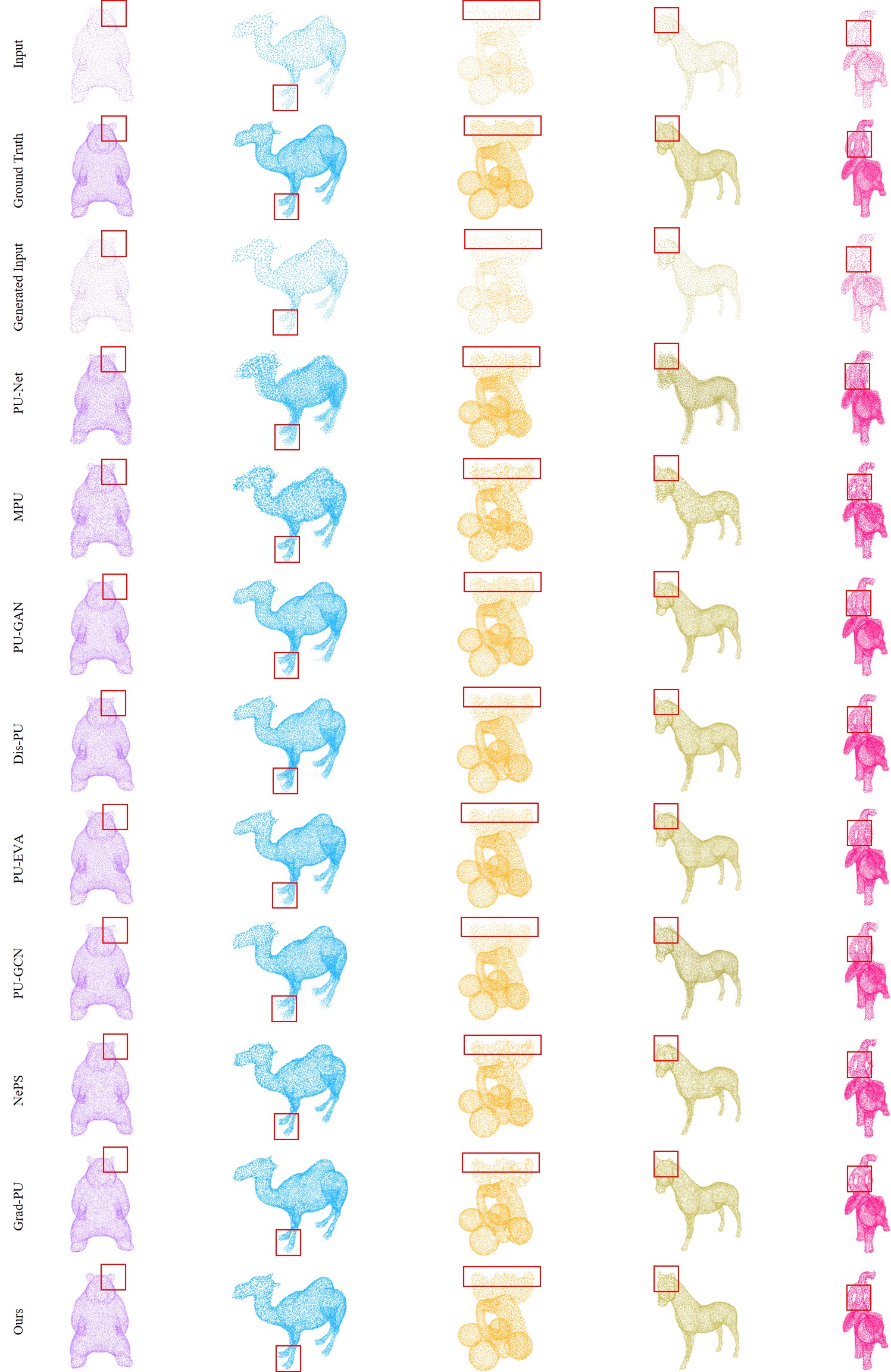
Figure 3: Visualization of point cloud upsampling at $4\times$ on PUGAN [17].

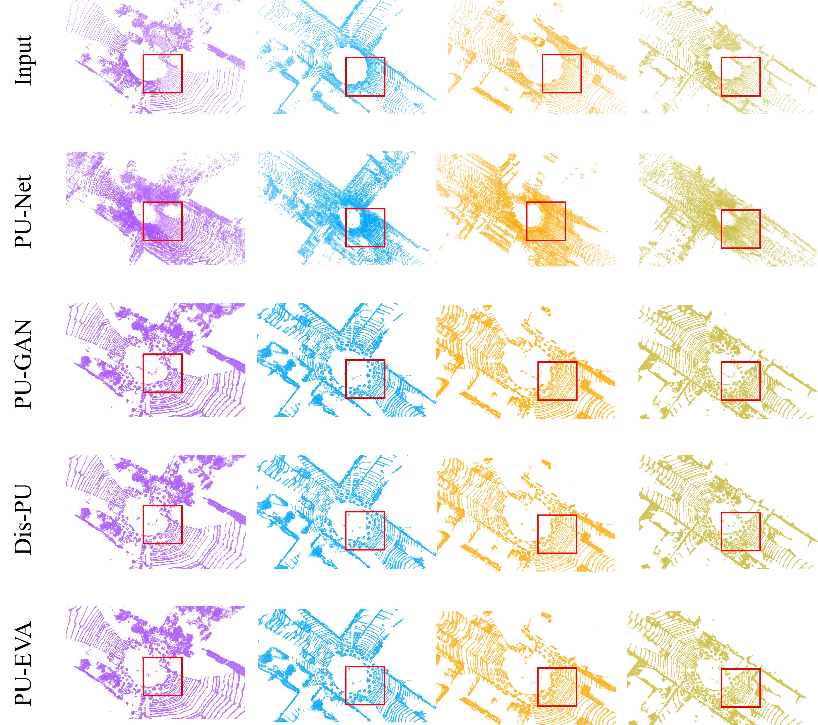
Figure 4: Visualization of point cloud upsampling at $4\times$ on KITTI [8].

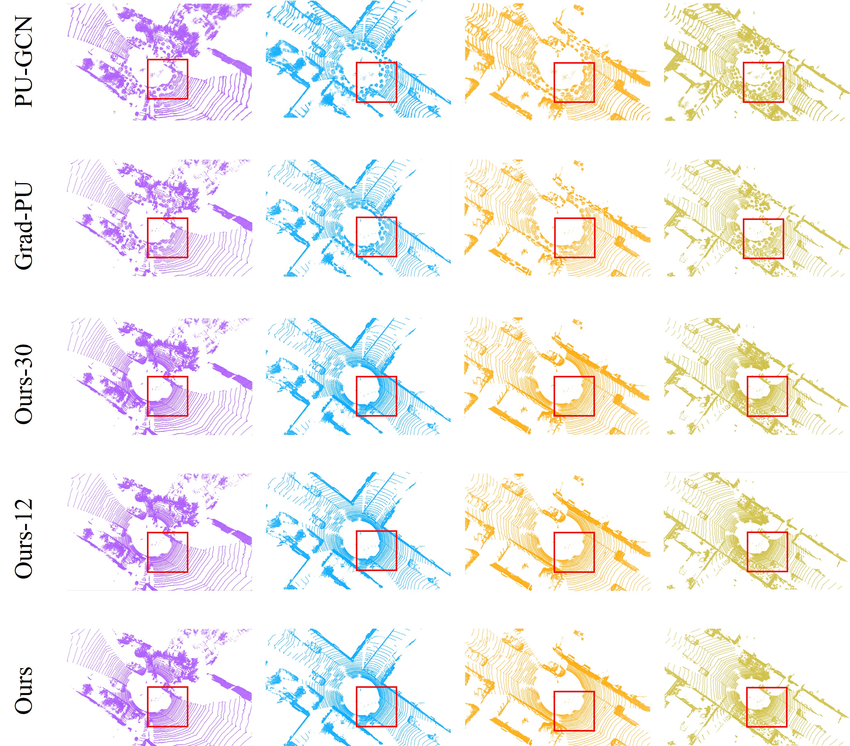
Figure 5: Visualization of point cloud upsampling at $4\times$ on KITTI [8]. ”Ours-12” and ”Ours-30” represent the results of our method at sampling intervals $=12$ and $=30$, respectively.

References

- Chang et al. [2015] Angel X Chang, Thomas Funkhouser, Leonidas Guibas, Pat Hanrahan, Qixing Huang, Zimo Li, Silvio Savarese, Manolis Savva, Shuran Song, Hao Su, et al. Shapenet: An information-rich 3d model repository. arXiv preprint arXiv:1512.03012, 2015.
- Choy et al. [2019a] Christopher Choy, JunYoung Gwak, and Silvio Savarese. 4d spatio-temporal convnets: Minkowski convolutional neural networks. In Proceedings of the IEEE/CVF conference on computer vision and pattern recognition, pages 3075–3084, 2019a.
- Choy et al. [2019b] Christopher Choy, Jaesik Park, and Vladlen Koltun. Fully convolutional geometric features. In Proceedings of the IEEE/CVF international conference on computer vision, pages 8958–8966, 2019b.
- Cui et al. [2021] Yaodong Cui, Ren Chen, Wenbo Chu, Long Chen, Daxin Tian, Ying Li, and Dongpu Cao. Deep learning for image and point cloud fusion in autonomous driving: A review. pages 722–739. IEEE, 2021.
- Dai et al. [2017] Angela Dai, Angel X Chang, Manolis Savva, Maciej Halber, Thomas Funkhouser, and Matthias Nießner. Scannet: Richly-annotated 3d reconstructions of indoor scenes. In Proceedings of the IEEE conference on computer vision and pattern recognition, pages 5828–5839, 2017.
- Dhariwal and Nichol [2021] Prafulla Dhariwal and Alexander Nichol. Diffusion models beat gans on image synthesis. Advances in neural information processing systems, 34:8780–8794, 2021.
- Feng et al. [2022] Wanquan Feng, Jin Li, Hongrui Cai, Xiaonan Luo, and Juyong Zhang. Neural points: Point cloud representation with neural fields for arbitrary upsampling. In Proceedings of the IEEE/CVF Conference on Computer Vision and Pattern Recognition, pages 18633–18642, 2022.
- Geiger et al. [2013] Andreas Geiger, Philip Lenz, Christoph Stiller, and Raquel Urtasun. Vision meets robotics: The kitti dataset. pages 1231–1237. Sage Publications Sage UK: London, England, 2013.
- He et al. [2023] Yun He, Danhang Tang, Yinda Zhang, Xiangyang Xue, and Yanwei Fu. Grad-pu: Arbitrary-scale point cloud upsampling via gradient descent with learned distance functions. In Proceedings of the IEEE/CVF Conference on Computer Vision and Pattern Recognition, pages 5354–5363, 2023.
- Ho and Salimans [2022] Jonathan Ho and Tim Salimans. Classifier-free diffusion guidance. arXiv preprint arXiv:2207.12598, 2022.
- Ho et al. [2020] Jonathan Ho, Ajay Jain, and Pieter Abbeel. Denoising diffusion probabilistic models. Advances in neural information processing systems, 33:6840–6851, 2020.
- Huang et al. [2021] Shengyu Huang, Zan Gojcic, Mikhail Usvyatsov, Andreas Wieser, and Konrad Schindler. Predator: Registration of 3d point clouds with low overlap. In Proceedings of the IEEE/CVF Conference on computer vision and pattern recognition, pages 4267–4276, 2021.
- Huang et al. [2022a] Sheng Yu Huang, Hao-Yu Hsu, and Frank Wang. Spovt: Semantic-prototype variational transformer for dense point cloud semantic completion. Advances in Neural Information Processing Systems, 35:33934–33946, 2022a.
- Huang et al. [2022b] Xiaoshui Huang, Sheng Li, Wentao Qu, Tong He, Yifan Zuo, and Wanli Ouyang. Frozen clip model is efficient point cloud backbone. arXiv preprint arXiv:2212.04098, 2022b.
- Huang et al. [2022c] Xiaoshui Huang, Wentao Qu, Yifan Zuo, Yuming Fang, and Xiaowei Zhao. Imfnet: Interpretable multimodal fusion for point cloud registration. IEEE Robotics and Automation Letters, 7(4):12323–12330, 2022c.
- Li and Lee [2021] Jiaxin Li and Gim Hee Lee. Deepi2p: Image-to-point cloud registration via deep classification. In Proceedings of the IEEE/CVF Conference on Computer Vision and Pattern Recognition, pages 15960–15969, 2021.
- Li et al. [2019] Ruihui Li, Xianzhi Li, Chi-Wing Fu, Daniel Cohen-Or, and Pheng-Ann Heng. Pu-gan: a point cloud upsampling adversarial network. In Proceedings of the IEEE/CVF international conference on computer vision, pages 7203–7212, 2019.
- Li et al. [2021] Ruihui Li, Xianzhi Li, Pheng-Ann Heng, and Chi-Wing Fu. Point cloud upsampling via disentangled refinement. In Proceedings of the IEEE/CVF conference on computer vision and pattern recognition, pages 344–353, 2021.
- Lin et al. [2018] Chen-Hsuan Lin, Chen Kong, and Simon Lucey. Learning efficient point cloud generation for dense 3d object reconstruction. In proceedings of the AAAI Conference on Artificial Intelligence, 2018.
- Liu et al. [2022] Kangcheng Liu, Yuzhi Zhao, Zhi Gao, and Ben M Chen. Weaklabel3d-net: A complete framework for real-scene lidar point clouds weakly supervised multi-tasks understanding. In 2022 international conference on robotics and automation (ICRA), pages 5108–5115. IEEE, 2022.
- Liu et al. [2019] Zhijian Liu, Haotian Tang, Yujun Lin, and Song Han. Point-voxel cnn for efficient 3d deep learning. Advances in Neural Information Processing Systems, 32, 2019.
- Luo et al. [2021] Luqing Luo, Lulu Tang, Wanyi Zhou, Shizheng Wang, and Zhi-Xin Yang. Pu-eva: An edge-vector based approximation solution for flexible-scale point cloud upsampling. In Proceedings of the IEEE/CVF International Conference on Computer Vision, pages 16208–16217, 2021.
- Luo and Hu [2021] Shitong Luo and Wei Hu. Diffusion probabilistic models for 3d point cloud generation. In Proceedings of the IEEE/CVF Conference on Computer Vision and Pattern Recognition, pages 2837–2845, 2021.
- Lyu et al. [2021] Zhaoyang Lyu, Zhifeng Kong, Xudong Xu, Liang Pan, and Dahua Lin. A conditional point diffusion-refinement paradigm for 3d point cloud completion. arXiv preprint arXiv:2112.03530, 2021.
- Melas-Kyriazi et al. [2023] Luke Melas-Kyriazi, Christian Rupprecht, and Andrea Vedaldi. Pc2: Projection-conditioned point cloud diffusion for single-image 3d reconstruction. In Proceedings of the IEEE/CVF Conference on Computer Vision and Pattern Recognition, pages 12923–12932, 2023.
- Pan et al. [2021] Liang Pan, Xinyi Chen, Zhongang Cai, Junzhe Zhang, Haiyu Zhao, Shuai Yi, and Ziwei Liu. Variational relational point completion network. In Proceedings of the IEEE/CVF conference on computer vision and pattern recognition, pages 8524–8533, 2021.
- Peebles and Xie [2023] William Peebles and Saining Xie. Scalable diffusion models with transformers. In Proceedings of the IEEE/CVF International Conference on Computer Vision, pages 4195–4205, 2023.
- Phan et al. [2018] Anh Viet Phan, Minh Le Nguyen, Yen Lam Hoang Nguyen, and Lam Thu Bui. Dgcnn: A convolutional neural network over large-scale labeled graphs. Neural Networks, 108:533–543, 2018.
- Qi et al. [2017a] Charles R Qi, Hao Su, Kaichun Mo, and Leonidas J Guibas. Pointnet: Deep learning on point sets for 3d classification and segmentation. In Proceedings of the IEEE conference on computer vision and pattern recognition, pages 652–660, 2017a.
- Qi et al. [2017b] Charles Ruizhongtai Qi, Li Yi, Hao Su, and Leonidas J Guibas. Pointnet++: Deep hierarchical feature learning on point sets in a metric space. Advances in neural information processing systems, 30, 2017b.
- Qian et al. [2021] Guocheng Qian, Abdulellah Abualshour, Guohao Li, Ali Thabet, and Bernard Ghanem. Pu-gcn: Point cloud upsampling using graph convolutional networks. In Proceedings of the IEEE/CVF Conference on Computer Vision and Pattern Recognition, pages 11683–11692, 2021.
- Qian et al. [2022] Guocheng Qian, Xingdi Zhang, Abdullah Hamdi, and Bernard Ghanem. Pix4point: Image pretrained transformers for 3d point cloud understanding. 2022.
- Qian et al. [2020] Yue Qian, Junhui Hou, Sam Kwong, and Ying He. Pugeo-net: A geometry-centric network for 3d point cloud upsampling. In European conference on computer vision, pages 752–769. Springer, 2020.
- Ramesh et al. [2021] Aditya Ramesh, Mikhail Pavlov, Gabriel Goh, Scott Gray, Chelsea Voss, Alec Radford, Mark Chen, and Ilya Sutskever. Zero-shot text-to-image generation. In International Conference on Machine Learning, pages 8821–8831. PMLR, 2021.
- Ramesh et al. [2022] Aditya Ramesh, Prafulla Dhariwal, Alex Nichol, Casey Chu, and Mark Chen. Hierarchical text-conditional image generation with clip latents. arXiv preprint arXiv:2204.06125, 1(2):3, 2022.
- Rombach et al. [2022] Robin Rombach, Andreas Blattmann, Dominik Lorenz, Patrick Esser, and Björn Ommer. High-resolution image synthesis with latent diffusion models. In Proceedings of the IEEE/CVF conference on computer vision and pattern recognition, pages 10684–10695, 2022.
- Saharia et al. [2022] Chitwan Saharia, William Chan, Saurabh Saxena, Lala Li, Jay Whang, Emily L Denton, Kamyar Ghasemipour, Raphael Gontijo Lopes, Burcu Karagol Ayan, Tim Salimans, et al. Photorealistic text-to-image diffusion models with deep language understanding. Advances in Neural Information Processing Systems, 35:36479–36494, 2022.
- Song et al. [2020a] Jiaming Song, Chenlin Meng, and Stefano Ermon. Denoising diffusion implicit models. arXiv preprint arXiv:2010.02502, 2020a.
- Song et al. [2020b] Yang Song, Jascha Sohl-Dickstein, Diederik P Kingma, Abhishek Kumar, Stefano Ermon, and Ben Poole. Score-based generative modeling through stochastic differential equations. arXiv preprint arXiv:2011.13456, 2020b.
- Thomas et al. [2019] Hugues Thomas, Charles R Qi, Jean-Emmanuel Deschaud, Beatriz Marcotegui, François Goulette, and Leonidas J Guibas. Kpconv: Flexible and deformable convolution for point clouds. In Proceedings of the IEEE/CVF international conference on computer vision, pages 6411–6420, 2019.
- Wu et al. [2021] Tong Wu, Liang Pan, Junzhe Zhang, Tai Wang, Ziwei Liu, and Dahua Lin. Balanced chamfer distance as a comprehensive metric for point cloud completion. Advances in Neural Information Processing Systems, 34:29088–29100, 2021.
- Wu et al. [2015] Zhirong Wu, Shuran Song, Aditya Khosla, Fisher Yu, Linguang Zhang, Xiaoou Tang, and Jianxiong Xiao. 3d shapenets: A deep representation for volumetric shapes. In Proceedings of the IEEE conference on computer vision and pattern recognition, pages 1912–1920, 2015.
- Xu et al. [2023] Jiale Xu, Xintao Wang, Weihao Cheng, Yan-Pei Cao, Ying Shan, Xiaohu Qie, and Shenghua Gao. Dream3d: Zero-shot text-to-3d synthesis using 3d shape prior and text-to-image diffusion models. In Proceedings of the IEEE/CVF Conference on Computer Vision and Pattern Recognition, pages 20908–20918, 2023.
- Yang et al. [2020] Lei Yang, Yanhong Liu, Jinzhu Peng, and Zize Liang. A novel system for off-line 3d seam extraction and path planning based on point cloud segmentation for arc welding robot. Robotics and Computer-Integrated Manufacturing, 64:101929, 2020.
- Yifan et al. [2019] Wang Yifan, Shihao Wu, Hui Huang, Daniel Cohen-Or, and Olga Sorkine-Hornung. Patch-based progressive 3d point set upsampling. In Proceedings of the IEEE/CVF Conference on Computer Vision and Pattern Recognition, pages 5958–5967, 2019.
- Yu et al. [2018] Lequan Yu, Xianzhi Li, Chi-Wing Fu, Daniel Cohen-Or, and Pheng-Ann Heng. Pu-net: Point cloud upsampling network. In Proceedings of the IEEE conference on computer vision and pattern recognition, pages 2790–2799, 2018.
- Yuksel [2015] Cem Yuksel. Sample elimination for generating poisson disk sample sets. In Computer Graphics Forum, pages 25–32. Wiley Online Library, 2015.
- Zhang et al. [2022] Renrui Zhang, Ziyu Guo, Wei Zhang, Kunchang Li, Xupeng Miao, Bin Cui, Yu Qiao, Peng Gao, and Hongsheng Li. Pointclip: Point cloud understanding by clip. In Proceedings of the IEEE/CVF Conference on Computer Vision and Pattern Recognition, pages 8552–8562, 2022.
- Zhao et al. [2021] Hengshuang Zhao, Li Jiang, Jiaya Jia, Philip HS Torr, and Vladlen Koltun. Point transformer. In Proceedings of the IEEE/CVF international conference on computer vision, pages 16259–16268, 2021.
- Zheng et al. [2022] Yuchao Zheng, Yujie Li, Shuo Yang, and Huimin Lu. Global-pbnet: A novel point cloud registration for autonomous driving. pages 22312–22319. IEEE, 2022.
- Zhou et al. [2021] Linqi Zhou, Yilun Du, and Jiajun Wu. 3d shape generation and completion through point-voxel diffusion. In Proceedings of the IEEE/CVF International Conference on Computer Vision, pages 5826–5835, 2021.