Spontaneous coupling of Q-learning algorithms in equilibrium

Abstract

Most contributions in the algorithmic collusion literature only consider symmetric algorithms interacting with each other. We study a simple model of algorithmic collusion in which Q-learning algorithms repeatedly play a prisoner’s dilemma and allow players to choose different exploration policies. We characterize behavior of such algorithms with asymmetric policies for extreme values and prove that any Nash equilibrium features some cooperative behavior. We further investigate the dynamics for general profiles of exploration policy by running extensive numerical simulations which indicate symmetry of equilibria, and give insight for their distribution.
Keywords: Algorithmic collusion, Q-learning, Reinforcement Learning, Multi Agent Reinforcement Learning.
JEL classification: C72, C63

1 Introduction

The growing use of pricing algorithms in various fields of the economy, as well as seminal work by Calvano et al, 2020 [1] and Klein, 2021 [2] have sparkled interest for algorithmic collusion. Q-learning algorithms, which constitute the building brick of numerous reinforcement learning algorithms, have indeed been reported to learn how to collude without communication. This has raised concerns, specifically for regulation policy purposes (Harrington, 2017 [3]), as well as theoretical questions at the intersection of economics and multi agent reinforcement learning literature.

In this paper, we investigate of Q-learning algorithms using different parameters and playing against each other interact. In our model, two Q-learning algorithms with an $\varepsilon$-greedy policy repeatedly play a parameterized Prisoner’s Dilemma. We use the same framework as Banchio and Mantegazza (2023)[4], who introduce the notion of spontaneous coupling to explain the observed tendency of Q-learning algorithms to learn dominated strategies in the long run. Intuitively, spontaneous coupling is a consequence of asynchronous updating (as also observed by Asker (2022) [5] and Banchio and Skrzypacz (2022) [6]), i.e. the fact that Q-values for an action are only updated when this action is played. Under spontaneous coupling, Q-learning algorithms alternate between phases of mutual cooperation and mutual defection. Schematically, the asynchronous nature of updating causes Q-values to increase (resp. decrease) when both players hold cooperation (resp. defection) as their preferred action. In the first case, Q-values for defection increase faster than those for cooperation, in the second, Q-values for defection decrease quicker than those for cooperation. For this last point to be true, and thus for spontaneous coupling to appear, cooperation must be played rarely enough when both agents prefer cooperation, that is the exploration parameter, $\varepsilon$, should be small enough. Banchio and Mantegazza (2023) prove this point formally using a continuous-time equivalent when algorithms use the same exploration policy. Since spontaneous coupling disappears for some values of the exploration parameter, a natural question is whether it remains in equilibrium, i.e., when algorithms’ designers compete using the parameters. We are thus interested in the equilibria of a game in which two algorithms designers simultaneously choose an exploration parameter, implement it in their respective algorithms, let them repeatedly play a prisoner’s dilemma on their behalf and collect the long-run payoffs.

Most of the known results on algorithmic collusion are simulation based, due to the difficulty of mathematically characterizing the complex interactions of several reinforcement learning algorithms. It is indeed well known in the literature on the topic that the theoretical guarantees that one has when a single Q-learning algorithm interacts with a stationary environment disappear with such interaction, so that, in order to investigate its properties, the use of extensive numerical simulations is necessary. Even when using simulations, the extend to which such interaction can be understood is generally limited to the capacity to represent outcomes visually, so that, to the best of our knowledge, situations featuring algorithms using different parameters have been left out. Remarkably, Banchio and Mantegazza (2023) are able to provide analytical results, however their proof relies on an assumption of symmetry in the initial conditions that we cannot use when considering different exploration policies.

To circumvent these difficulties, we analytically characterize the behavior of the algorithms for extreme values of parameters, specifically in three cases that make their interaction predictable: (i) when one of them uses $\varepsilon=1$ (i.e. explores all the time) (ii) when one of them uses $\varepsilon_{A}=0$ and the other uses $\varepsilon_{B}>0$ (i.e. when $A$ only exploits) and (iii) when both use $\varepsilon=0$. In the first two cases, we show spontaneous coupling disappears, whereas in the third it remains possible.

We then perform extensive numerical simulations to investigate the behavior of algorithms for general profiles of exploration parameters Their results reveal the dynamics are not different in essence than the ones uncovered by Banchio and Manteggazza (2023), spontaneous coupling appearing for moderate $\varepsilon$s. For such parameters, the algorithms spend positive time holding cooperation as a preferred action, so that four regimes are to be distinguished: $CC$, when both algorithms prefer cooperation, $DD$ when both prefer defection and $DC$/$CD$ when their preferences are opposed. These should be distinguished from the probability with which spontaneous coupling is reached, which depends on the initial conditions used by the algorithms. Using simple clustering techniques (namely K-means) we are able to measure this probability so as to independently measure the time spent in the different regimes (conditional on reaching spontaneous coupling).

Allowing $\varepsilon$s to be set in a strategic fashion sheds light on the fact that more exploration is unilaterally profitable conditional on cycles featuring spontaneous coupling, as it allows to exploit the other player when both currently hold cooperation for a best action. However, extra cooperation comes at the cost of potentially destroying the spontaneous coupling, which is detrimental. We build on this simple idea to get theoretical results on equilibria, leveraging results concerning extreme values of parameters. Specifically, we prove that (i) the profile $(\varepsilon_{A}=0,\varepsilon_{B}=0)$ is a Nash equilibrium and (ii) any Nash equilibrium features spontaneous coupling. Further simulations indicate that Nash equilibria are generally symmetric and are located on a bell-shaped curve with respect to a parameter controlling both the incentive to deviate from mutual cooperation and the extend to which mutual cooperation is beneficial compared to mutual defection.

The rest of the paper is organized as follows. Section 2 reviews the literature related to the present work, Section 3 presents Q-learning as well as our setting, Section 4 presents our analytical results regarding extreme exploration policies ($\varepsilon\in\{0,1\}$) and Nash equilibria, Section 5 and 6 describe the simulation used to investigate more general policies and present their results, Section 7 concludes.

2 Related literature

The possibility of spontaneous collusion by Q-learning algorithms has been receiving important attention in recent years. On the empirical side, Assad et al, 2020 [7] have provided evidence for algorithmic collusion in the German gasoline retail market in which algorithmic pricing methods became widely available in 2017. A similar phenomenon has been highlighted by Musolff et al, 2022 [8] using Amazon data. The policy implications and practical relevance of the topic are discussed in Calvano et al, 2019 [9]. On the theoretical side, the seminal contributions are those of Calvano et al, 2020 [1] and of Klein, 2021 [2]. Using extensive simulations, they show that Q-learning algorithms playing a repeated pricing game (in a Bertrand oligopoly in the first case, in a setting à la Maskin and Tirole, 1988 [10] in the second) learn to set supra-competitive prices in the long run. Calvano et al (2020) emphasize the anatomy of collusion constituted by punishment-reward schemes upon deviation, which is made possible by letting algorithms condition their play on the previous action played by their opponent. In Klein (2021) on the other hand, long run behavior is characterized by asymmetric cycling prices rotating demand between players. Simulation-based extension have followed. Calvano et al, 2021 [11] consider a setting with a Cournot duopoly with stochastic demand and show that a similar collusive behavior appears. Banchio and Skrzypacz, 2022 [6] consider Q learning algorithms repeatedly playing classical auction games, and interestingly report a difference between second price and first price auctions: in second price auctions, algorithms converge to the static equilibrium of the stage game, while in first price auction collusive behavior appears. Hettich, 2021 [12] runs simulations using a more advanced technology (namely deep Q-learning, see Mnih et al, 2015 [13] for a description of this deep reinforcement learning method) provide similar results than Calvano et al (2020) with a way faster convergence to collusive behavior, which motivates further research on the topic of algorithmic collusion. Further extensions have been considered, typically by investigating the role of different market structures as in Sanchez-Cartas and Katsamakas, 2022 [14], or in Abada and Lambin, 2022 [15], which find similar results than Calvano et al (2020) on an economic environment replicating electricity markets. Further, Johnson et al, 2022 [16] study the effect of platform design on the behavior of Q-learning algorithms. They specifically show that some platform designs that are effective for classical players turns out to be socially harmful when Q-learning algorithms are there, and point out a different, more adapted, one.

Another branch of research, which the present work mostly builds on, have focused on understanding the mechanism responsible for collusion. By simulating stateless Q-learning algorithms with $\varepsilon$-greedy policies, Asker et al, 2022 [5] provide evidence that collusive behavior is rooted in Q-learning’s asynchronous updating, and highlight that if algorithms have access to minimal information and are given minimal economic reasoning (specifically the demand being downward sloping), then collusion is reduced by a lot. Similar phenomenon is observed by Banchio and Skrzypacz (2022) : letting Q-learning have access to the highest bid in previous period and letting them compute counterfactual scenarios when updating Q-values make collusive behavior disappear. Finally, the contribution we build on most is this of Banchio and Mantegazza, 2022 [4], which characterizes limiting behavior of the Q-learning algorithms playing a repeated prisoner’s dilemma using continuous time equivalents. More precisely, they provide a theoretical bound on exploration level under which collusive behavior is possible. They highlight a phenomenon of spontaneous coupling between $\varepsilon$-greedy algorithms, and formally prove that letting algorithms synchronously update the Q-values prevents collusion.

The aforementioned contributions do not, in general, study settings with competition on the algorithms. A notable exception is Sanchez-Cartas and Katsamakas (2021), who compare Q-learning with Particle Swarm Optimization (PSO, a meta-heuristic method of optimization first described by Kennedy and Eberhart, 1995 [17]). Their simulations indicate that, when PSO is competing with a stateless Q-learning algorithm both set supracompetitive prices, but do not consider the different technologies as being chosen in order to compete between each other. To the best of our knowledge, only Compte, 2023 [18] integrates equilibrium considerations. In this paper, a variation of Q-learning integrating a possible bias towards cooperation is considered, such a bias being chosen simultaneously by players before algorithms start running. Simulations using a prisonners’ dilemma indicate that Nash equilibria featuring positive bias towards cooperation exist and enhance collusive behavior.

More generally, the present work relates to a broader literature on Multi Agent Reinforcement Learning (MARL), which lies at the interface of computer science and game theory, an introduction to which is given by Nowé et al, 2012 [19]. MARL presents the difficulty of having very few theoretical guarantees on the convergence of algorithms. Particularly, important contributions in the field have focused on designing algorithms that extend classical Q-learning, such as Tesauro, 2003 [20] with Hyper Q-learning and Hu, 2003 [21] with Nash Q-learning. More specifically, other authors have focused on building agents that maintain cooperation in prisoner’s dilemma like environment by adapting modern reinforcement learning techniques, such as Lere and Peysakhovich, 2017 [22] and Tampuu et al, 2017 [23]. Closer to our interest, Kianercy and Galstyan, 2012 [24] provide a full characterization of the rest points of a system composed of two Q-learning algorithms with Boltzmann exploration policy playing $2\times 2$ games. Generally, it is well-known that some algorithms tend to learn cooperation when repeatedly playing a prisoner’s dilemma, see Banerjee and Sen, 2007 [25] for an example.

3 Setting and notations

3.1 Q-learning

Q-learning is a simple reinforcement learning principle designed to find optimal solutions to optimization problems in a Markov environment. Formally, denote $S$ a (finite) set of states, $A$ a set of actions and $\pi(s,a)$ the (possibly stochastic) reward obtained in state $s$ after taking action $a$. In each period, an action is taken, a reward is realized and the process moves to the next state with a probability $F(s_{t+1}|s_{t},a_{t})$. The objective is to learn the best policy, i.e. the one that maximizes $\mathbb{E}\Big{[}\sum_{t=0}^{+\infty}\gamma^{t}\pi_{t}\Big{]}$ with $\gamma\in(0,1)$ an discount rate, without any information about the transition function $F$. Classically, one can write the Bellman value function as follows:

$$\forall s\in S,V(s)=\mathbb{E}(\pi(s,a))+\gamma\mathbb{E}(V(s^{\prime})).$$ (1)

The Q-matrix is defined as

$$\forall(s,a)\in A\times S,Q(s,a)=\mathbb{E}[\pi|s,a]+\gamma\mathbb{E}[\max_{\{a^{\prime}\in A\}}Q(s^{\prime},a^{\prime})|s,a],$$ (2)

and linked to the Bellman value function as follows

$$V(s)=\max_{a\in A}Q(s,a).$$ (3)

Put differently, an agent who knows the Q-matrix exactly knows what action to take in each state, and thus knows the optimal policy. Q-learning estimates this matrix by an iterative procedure. The agent begins with an arbitrary $Q_{0}$ and updates any cell of the matrix she visits as follows:

$$Q_{t+1}(s,a)=(1-\alpha)Q_{t}(s,a)+\alpha\Big{[}\pi_{t}+\gamma\max_{a^{\prime}\in A}Q_{t}(s^{\prime},a)\Big{]},$$ (4)

where $\alpha$ is referred to as the learning rate and controls how rapidly Q-values change when a reward is obtained. Note that when $\alpha=0$ the Q-values stay constant, so that the agent does not learn, and when $\alpha=1$ the Q-values immediately change to the actualized reward. To decide which action to take given a matrix of Q-values, the agent relies on an exploration policy. The two most common exploration policies are Boltzmann and $\varepsilon$-greedy.

Under Boltzmann exploration policy, the agent chooses an action $a$ in state $s$ with the probability

$$\mathbb{P}(a|s)=\frac{\exp\big{(}\lambda Q_{t}(s,a)\big{)}}{\sum_{a^{\prime}\in A}\exp\big{(}\lambda Q_{t}(s,a^{\prime})\big{)}},$$ (5)

where $\lambda$ is a parameter controlling for the balance between exploration and exploitation. When $\lambda=0$ the agent always chooses an action uniformly at random (i.e. spends her time exploring), whereas when $\lambda\to+\infty$ she always chooses the action with the highest Q-value (i.e. spends her time exploiting).

The policy we focus on is $\varepsilon$-greedy, under which the action chosen at time $t$ in state $s$ is

$$a_{t}(s)=\left\{\begin{array}[]{ll}\arg\max_{a^{\prime}}Q_{t}(a^{\prime},s)\text{ with probability }1-\varepsilon\\ \sim\mathcal{U}(A)\text{ with probability }\varepsilon.\end{array}\right.$$ (6)

The $\varepsilon$ parameter here plays a similar role than $\lambda$ for the Boltzmann policy. The higher $\varepsilon$ the more frequently the agent explores, so that for $\varepsilon=1$ the agent always chooses uniformly at random. Conversely, when $\varepsilon=0$ the agent always chooses the action with highest Q-value, i.e. is greedy.

Under mere assumptions on the learning rates and on the exploration policy, $Q_{t}$ converges to the Q-matrix with probability $1$ (Watkins and Dayan, 1992) [26]. Though, when several Q-learning algorithms interact, it is well known that this result does not hold anymore: as each algorithm reacts to the other’s learning, their environment becomes evolving and they face a moving target problem preventing them to eventually learn an optimal policy.

3.2 Notations and hypothesis

3.2.1 Stage game

As in Banchio and Mantegazza (2023), the game that is repeatedly played by the Q-learning algorithms is a Prisoner’s Dilemma the payoff matrix of which is presented in Table 1. We will denote this game $G_{0}(g)$, and $\tilde{\pi}^{P}_{X,Y}$ the payoff player $P$ gets under profile of actions $(X,Y)$ in $G_{0}(g)$. The parameter $g$ takes values in $[1,2]$ and has a twofold effect on the game. First, note how $\tilde{\pi}^{A}_{CC}-\tilde{\pi}^{A}_{DD}=2(g-1)$, so that when $g$ increases mutual defection becomes more socially detrimental. Conversely, one can see that when $g=1$, $\tilde{\pi}^{A}_{CC}=\tilde{\pi}^{A}_{DD}$ so that there is no social cost to mutual defection. Second, note how $\tilde{\pi}^{A}_{DC}-\tilde{\pi}^{A}_{CC}=2-g$ is decreasing with $g$. Thus, the incentive to deviate from mutual cooperation is decreasing with $g$ and eventually is null when $g=2$.

		Player $B$
		$C$	$D$
Player $A$	$C$	$2g,2g$	$g,2+g$
	$D$	$g,2+g$	$2,2$

Table 1: Payoffs in the parameterized Prisoner’s Dilemma

3.2.2 Game on exploration parameters

We will assume players $A$ and $B$ use Q-learning algorithms to repeatedly play the stage game $G_{0}(g)$ repeatedly. Prior to letting algorithms play on their behalf, they need to simultaneously choose an exploration parameter $\varepsilon_{A},\varepsilon_{B}\in[0,1]$, implement it in their algorithm, let it play over a long enough period of time and collect the payoff obtained in the limit. We call this game $G(g)$ Note that whether algorithms converge or not is a highly non trivial question. Even though there are no theoretical guarantees, we will assume they do and leave this question out of the scope of this paper. Our simulations generally confirm this hypothesis. The evolution of Q-values is intrinsically stochastic thus, a priori, convergence to spontaneous coupling and the behavior under spontaneous coupling remains stochastic. We define the following objects and quantities to help clarify the payoff function.

Definition 1.

For $P\in\{A,B\}$, $X\in\{C,D\}$, we denote $\omega_{X}^{P}=\{\mathbb{Q}=(Q_{A}^{C},Q_{A}^{D},Q_{B}^{C},Q_{B}^{D})\in\mathbb{R^{4}}\text{ s.t. }Q_{X}^{P}>Q_{-X}^{P}\}$ where $-X=C$ when $X=D$ and vice-versa. Further, for $X,Y\in\{X,Y\}$ we denote $\omega_{X,Y}=\omega_{X}^{A}\cap\omega_{Y}^{B}$.

Definition 2.

For all $X,Y\in\{C,D\}$, we let $\tau^{g}_{X,Y}(\varepsilon_{A},\varepsilon_{B})\in[0,1]$ the average fraction of time spent in region $\omega_{X,Y}$ in the long run when repeatedly playing $G_{0}(g)$. More formally, if at $t$ the system has reached its limit behavior:

$$\tau^{g}_{X,Y}(\varepsilon_{A},\varepsilon_{B})=\mathbb{P}(\mathbb{Q}_{t}\in\omega_{X,Y})$$ (7)

Definition 3.

For all $X,Y$, we let $\pi^{P}_{X,Y}(\varepsilon_{A},\varepsilon_{B})$ be the average payoff player $P$ gets when in zone $\omega_{X,Y}$, so that :

$$\left\{\begin{array}[]{ll}\pi^{A}_{C,C}=(1-\frac{\varepsilon_{A}}{2})(1-\frac{\varepsilon_{B}}{2}).2g+(1-\frac{\varepsilon_{A}}{2})\frac{\varepsilon_{B}}{2}.g+\frac{\varepsilon_{A}}{2}(1-\frac{\varepsilon_{B}}{2}).(2+g)+\frac{\varepsilon_{A}}{2}\frac{\varepsilon_{B}}{2}.(2)\\ \pi^{A}_{C,D}=(1-\frac{\varepsilon_{A}}{2})(1-\frac{\varepsilon_{B}}{2}).g+(1-\frac{\varepsilon_{A}}{2})\frac{\varepsilon_{B}}{2}.2g+\frac{\varepsilon_{A}}{2}(1-\frac{\varepsilon_{B}}{2}).2+\frac{\varepsilon_{A}}{2}\frac{\varepsilon_{B}}{2}.(2+g)\\ \pi^{A}_{D,C}=(1-\frac{\varepsilon_{A}}{2})(1-\frac{\varepsilon_{B}}{2}).(2+g)+(1-\frac{\varepsilon_{A}}{2})\frac{\varepsilon_{B}}{2}.2+\frac{\varepsilon_{A}}{2}(1-\frac{\varepsilon_{B}}{2}).2g+\frac{\varepsilon_{A}}{2}\frac{\varepsilon_{B}}{2}.g\\ \pi^{A}_{D,D}=(1-\frac{\varepsilon_{A}}{2})(1-\frac{\varepsilon_{B}}{2}).2+(1-\frac{\varepsilon_{A}}{2})\frac{\varepsilon_{B}}{2}.(2+g)+\frac{\varepsilon_{A}}{2}(1-\frac{\varepsilon_{B}}{2}).g+\frac{\varepsilon_{A}}{2}\frac{\varepsilon_{B}}{2}.2g\end{array}\right.$$ (8)

Then we can write the payoff function of $A$ in $G(g)$ as

$$\Pi^{A}(\varepsilon_{A},\varepsilon_{B})=\sum_{(X,Y)\in\{C,D\}^{2}}\tau^{g}_{X,Y}(\varepsilon_{A},\varepsilon_{B})\pi^{A}_{X,Y}(\varepsilon_{A},\varepsilon_{B})$$ (9)

The corresponding quantities for $B$ are easily deduced by symmetry.

3.2.3 Initial conditions

It is worth noting that the process on Q values is Markovian, so that $\mathbb{Q}_{t}$ only depends on $\mathbb{Q}_{t-1}$. Though, the process might not be ergodic and thus depend on the initial conditions. In this work, we choose to focus on exploration parameters and thus we do not consider initial condition to be chosen strategically. To simplify things, we restrict attention to specific, well chosen intervals from which initial conditions are uniformly drawn, which we justify by the following result:

Proposition 1.

Assume $\varepsilon_{A},\varepsilon_{B}>0$. Then with probability $1$ there exists $t$ such that:

$$\forall P\in\{A,B\},\forall X\in\{C,D\},Q_{P}^{X}(t)\in[\frac{\tilde{\pi}^{P}_{X,D}}{1-\gamma},\frac{\tilde{\pi}^{P}_{X,C}}{1-\gamma}]\equiv I_{X}.$$ (10)

This proposition pins down an interval for each action, denoted $I_{X}$, in which the process is guaranteed to end up at some point. Their bounds correspond to the actualized lowest and highest payoffs action $X$ can yield when played, i.e. when the other player plays $D$ in the first case and $C$ in the second. In some sense then, these intervals corresponds to the ”natural” values Q-values can take. Even though the process is not necessarily ergodic, we make the simplifying assumption that initial conditions for Q-values are uniformly drawn in those intervals. In the following, we denote $\mathbb{I}=(I_{C}\times I_{D})^{2}$

3.3 Former results

The behavior of two interacting Q-learning algorithms is complex so that a useful object to rely on is its continuous time approximation. Intuitively, the continuous time approximation of Q-values is the limit behavior of a similar system updated infinitely many times per period, each update having a negligible effect (see Banchio and Mantegazza (2023) Sec. 2.2) for a formal presentation). In order to distinguish the stochastic process generated by the actual Q-values (in discrete time) from its continuous time equivalent, we will denote the latter $\big{(}\tilde{\mathbb{Q}_{t}}\big{)}_{t\in\mathbb{R}}=\Bigg{(}\Big{(}\tilde{Q}_{A}^{C}(t),\tilde{Q}_{A}^{D}(t),\tilde{Q}_{B}^{C}(t),\tilde{Q}_{B}^{D}(t)\Big{)}\Bigg{)}_{t\in\mathbb{R}}$ as opposed to $\big{(}\mathbb{Q}_{t}\big{)}_{t\in\mathbb{N}}$. In region $\omega_{X,Y}$ the dynamics of the continuous time approximation for the Q-values of player $A$ can be written as:

$$\left\{\begin{array}[]{ll}\dot{\tilde{Q}}_{A}^{X}(t)=\alpha\big{(}1-\frac{\varepsilon_{A}}{2}\big{)}\Big{[}\hat{\pi}_{X,Y}-(1-\gamma)\tilde{Q}_{A}^{X}(t)\Big{]}\\ \dot{\tilde{Q}}_{A}^{-X}(t)=\alpha\frac{\varepsilon_{A}}{2}\Big{[}\hat{\pi}_{-X,Y}+\gamma\tilde{Q}_{A}^{X}(t)-\tilde{Q}_{A}^{-X}(t)\Big{]},\end{array}\right.$$ (11)

where $\hat{\pi}_{X,Y}$ is the average payoff player $A$ gets when she plays action $X$ while in region $\omega_{X,Y}\cup\omega_{-X,Y}$, i.e.

$$\hat{\pi}_{X,Y}=\big{(}1-\frac{\varepsilon_{B}}{2}\big{)}\tilde{\pi}_{X,Y}+\frac{\varepsilon_{B}}{2}\tilde{\pi}_{X,-Y}.$$ (12)

Under the assumption of symmetry in the initial condition (i.e. $\forall X\in\{C,D\},\tilde{Q}_{A}^{X}(0)=\tilde{Q}_{B}^{X}(0)$), the continuous time equivalents remain in $\omega_{CC}\cup\omega_{DD}$, allowing Banchio and Mantegazza (2023) to prove the following result in the case $\varepsilon_{B}=\varepsilon_{A}=\varepsilon$:

Proposition 0 (Banchio and Mantegazza).

Let $\underline{\varepsilon}(g)=1-\sqrt{\frac{2-g}{g}}$. If $\varepsilon>\underline{\varepsilon(g)}$ then all initial condition lead to $Q_{D}^{\text{eq}}=\Big{(}\frac{2\varepsilon+2g-\varepsilon g}{2}+\frac{\gamma(4+\varepsilon g}{2(1-\gamma)},\frac{4+\varepsilon g}{2(1-\gamma)}\Big{)}\in\omega_{DD}$. If $\varepsilon\leq\underline{\varepsilon(g)}$ a pseudo steady-state $Q_{C}^{\text{eq}}$ exists and lies in $\omega_{CC}$.

The identification of this pseudo steady-state relies on the piece wise linearity of the dynamics and on the concept of Filippov solutions [27] to such systems of differential equations. Intuitively, a Filippov solution appears when the flow of the system has opposite directions along a border causing it to cycle between two regions. In our case, this translates into the Q-values alternating between phases in $\omega_{CC}$ and $\omega_{DD}$. Schematically, in $\omega_{CC}$ phases, Q-values for both $C$ and $D$ increase, however Q-values for $D$ tend to increase faster causing the system to eventually go back to $\omega_{DD}$. in $\omega_{DD}$ phases, Q-values for both $C$ and $D$ decrease, leaving a possibility to transition from $\omega_{DD}$ back to $\omega_{CC}$. Such alternating behavior is in some sense ”broken” by too high exploration policies. This can be understood as follows: for those cycles to happen, the Q-values for $C$ should not decrease too fast when the system is in $\omega_{DD}$, otherwise it will not switch to $CC$ again. For this not to happen, the frequency of exploration should be low enough so as for $C$ not to be played (and thus updated) too often during $\omega_{DD}$ phases. Intuitively as well, the higher $\varepsilon$, the shorter should be the time spent in $\omega_{CC}$ as it increases the frequency with which Q-values for $D$ are updated and thus the speed with which they increase. Following the terminology introduced by Banchio and Mantegazza, we will refer to this phenomenon as spontaneous coupling.

3.4 Spontaneous coupling in the general case

In the general case, i.e. when exploration parameters are different, the continuous time equivalent can be studied region by region, allowing to get the following simple result

Proposition 2.

$\forall(\varepsilon_{A},\varepsilon_{B},g)\in[0,1]\times[0,1]\times[1,2]$, there exists a steady state $\tilde{\mathbb{Q}}^{\text{eq}}_{DD}$ of the continuous time equivalent that lies in $\omega_{DD}$. No other steady-state exists.

This is simply obtained by setting the flow of the continuous time equivalent in $\omega_{DD}$ to $0$ and checking the solution lies in $\omega_{DD}$, while setting it to $0$ in any other region yields a contradiction (more precisely it gives a solution outside the concerned region). Thus, for all parameterizations, we should expect a non-spontaneous coupling outcome to be possible. Naturally, we would like to extend Banchio and Mantegazza’s reasoning to the general case and look for Filippov solutions of the continuous time equivalent. This however is not possible as the hypothesis of symmetry in the initial conditions no longer guarantees the system to stay in $\omega_{CC}\cup\omega_{DD}$. This prevents Filippov solutions to be defined as it would require defining a sliding vector on a surface of co-dimension $2$, which, as well known in the specialized literature (see Dieci et al (2011, 2013) [28, 29] ) is not generally possible. We thus cannot give a definition of spontaneous coupling as the existence of a Filippov pseudo-equilibrium of the continuous time equivalent. To circumvent this difficulty, we give the following definition to spontaneous coupling:

Definition 4.

Let $(\varepsilon_{A},\varepsilon_{B},g)\in[0,1]\times[0,1]\times[1,2]$. We say $(\varepsilon_{A},\varepsilon_{B},g)$ allows for spontaneous coupling iff there exists $\mathbb{Q}_{0}\in\mathbb{R}^{4}$ such that:

$$\forall S\subset\mathbb{R}^{4}\text{ s.t. },\mathbb{P}(\exists t\in\mathbb{N},\mathbb{Q}_{t}\in S)=1,\exists\tilde{\mathbb{Q}}_{0}\in S\text{ s.t. }\neg\Bigg{(}\lim_{+\infty}\tilde{\mathbb{Q}}_{t}(\varepsilon_{A},\varepsilon_{B},g,\tilde{\mathbb{Q}}_{0})\in\omega_{DD}\Bigg{)}.$$ (13)

Further, we define the basin of attraction of spontaneous coupling as

$$\mathcal{B}(\varepsilon_{A},\varepsilon_{B},g)=\{\tilde{\mathbb{Q}}_{0}\in\mathbb{I}s.t.\lim_{+\infty}\tilde{Q}_{t}(\varepsilon_{A},\varepsilon_{B},g;\tilde{\mathbb{Q}_{0}})\neq\tilde{\mathbb{Q}}_{DD}^{\text{eq}}\}$$ (14)

and its size as

$$\mathcal{S}(\varepsilon_{A},\varepsilon_{B},g)=\lambda(\mathcal{B}(\varepsilon_{A},\varepsilon_{B},g))$$ (15)

where $\lambda(.)$ is the Lebesgue measure on $\mathbb{R}^{4}$.

Note that we use both the (discrete) dynamics of Q-learning algorithms and their continuous counter part in order to define spontaneous coupling. Intuitively, the continuous time equivalent describes what happens when algorithms update like they would do ”on average”, however, when $\varepsilon_{A}=0$ or $\varepsilon_{B}=0$ the actual dynamics of Q-learning algorithms are affected by rare events, causing the continuous time equivalent to poorly describe them. In our definition, we thus require that in the long run, the ”averaged version” of the system feature some time spent in any other region than $\omega_{DD}$ and the actual system doesn’t get stuck in $\omega_{DD}$.

4 Behavior of the system for extreme parameters

As a first step, we seek to characterize the behavior of the algorithms when one of the players adopt an extreme exploration parameter ($\varepsilon\in\{0,1\}$). In those cases, the system becomes more easily predictable which allows us to get analytical results on the possibility of spontaneous coupling.

Proposition 3.

For any $g\in[0,1]$, if $\varepsilon_{A}=1$ or $\varepsilon_{B}=1$, $(\varepsilon_{A},\varepsilon_{B},g)$ does not allow for spontaneous coupling.

The intuition for this result is the following. Whenever one player (say $A$) adopts $\varepsilon=1$, her behavior becomes constant over time, i.e. she always fully randomizes between the two actions. As a consequence, the environment for the $B$ becomes stationary, causing him to learn to defect in the long run. This remains true for any value of $\varepsilon_{B}$, especially for $\varepsilon_{B}=1$, which is in line with Banchio and Mantegazza’s result.

We get a similar result in the case $\varepsilon_{A}=0$ and $\varepsilon_{B}>0$:

Proposition 4.

For any $g\in[0,1]$, if $\varepsilon_{A}=0$ and $\varepsilon_{B}>0$, $(\varepsilon_{A},\varepsilon_{B},g)$ does not allow for spontaneous coupling.

In this case, one player is fully greedy while the other uses a non-zero exploration parameter. This result is somehow counter-intuitive given the known boundary on exploration parameters that allow for spontaneous coupling in the symmetric case and relies on the sensitivity of the system to rare events. Consider that, the Q-values of player $A$ behave in a very predictable way. Since she is fully greedy, she only plays actions with the highest Q-value, and thus only this one is updated at any period. We should also note that, whenever player $B$ plays $C$ (resp. $D$), the Q-value of the action $A$ holds as preferred increases (resp. decreases), and that $Q_{A}^{D}$ can never decrease below $\frac{2}{1-\gamma}$ while $Q_{A}^{C}$ can. Now assume at some point in time, her Q-value for $C$ is above her Q-value for $D$. She keeps on playing $C$, causing $Q_{A}^{C}$ to increase whenever $B$ plays $C$ and to decrease whenever $B$ plays $D$. Thus, if $B$ plays $D$ several times in a row for long enough, $Q_{A}^{C}$ will eventually decrease until it goes under $Q_{A}^{D}$. As long as $Q_{A}^{D}$ and $Q_{A}^{C}$ remain in the interval $[\frac{2}{1-\gamma},\frac{2g}{1-\gamma}]$, $Q_{A}^{D}$ and $Q_{A}^{C}$ will sequentially undercut each other, until eventually $Q_{A}^{C}$ goes below $\frac{2}{1-\gamma}$ causing $Q_{A}^{C}$ to remain below $Q_{A}^{D}$ from this time on. Once this happens, the behavior of $A$ becomes stationary: she only plays $D$, causing $B$ to adapt and learn $D$ in the long run as well. Note how, in this case, the result relies on the occurrence of rare events with certainty over a long period of time, so that the continuous time equivalent poorly describe the actual dynamics of the system.

Finally, we partially characterize the behavior of the system when $\varepsilon_{A}=\varepsilon_{B}=0$, that is when both algorithms are greedy.

Proposition 5.

For any $g$, $(0,0,g)$ allows for spontaneous coupling. More specifically for any initial condition in $\mathbb{I}$, there exists $t^{*}\in\mathbb{N}$ such that for all $t>t^{*},\mathbb{Q}(t)\in\omega_{CC}$ or $t^{*}\in\mathbb{N}$ such that for all $t>t^{*},\mathbb{Q}(t)\in\omega_{DD}$. Furthermore, $\tau^{g}_{CC}(0,0)\geq 4\Big{(}1-\frac{1}{g}\Big{)}^{4}\in[0,\frac{1}{4}]$.

In this case, the system is completely deterministic and fully determined by the initial condition. Specifically, we note that when the system gets in $\omega_{CC}$ it remains in $\omega_{CC}$, which allow us to get the lower bound on $\tau^{g}_{CC}(0,0)$. A argument similar to the one used in the case $\varepsilon_{A}=0$ and $\varepsilon_{B}>0$ allows to deduce that if the system never enters $\omega_{CC}$ it needs to remain in $\omega_{DD}$.

5 General properties of $G(g)$

The previous results concerning the possibility of spontaneous coupling for extreme values of parameters allow us to draw conclusions concerning the game $G(g)$.

Proposition 6.

For all $g\in[1,2]$, $(\varepsilon_{A}=0,\varepsilon_{B}=0)$ is a Nash equilibrium of $G(g)$. It is strict whenever $g>1$.

Proof.

Assume $\varepsilon_{B}=0$, then if $A$ chooses $\varepsilon_{A}>0$, $\tau^{g}_{DD}(\varepsilon_{A},\varepsilon_{B})=1$ (Proposition 4). Then $A$ receives payoff:

$$\Pi^{A}(\varepsilon_{A},0)=2(1-\frac{\varepsilon_{A}}{2})+g\frac{\varepsilon_{A}}{2}\leq 2.$$ (16)

However, if $A$ uses $\varepsilon_{A}=0$ then she gets payoff

$$\Pi^{A}(0,0)=2\tau_{DD}^{g}(0,0)+2g\tau_{CC}^{g}(0,0)\geq 2.$$ (17)

We deduce the result by symmetry of the game. ∎

Loosely speaking, if player $A$ were to know there will not be spontaneous coupling, playing $\varepsilon_{A}>0$ is under optimal. Since in this case both algorithms will learn $D$, it is clear that any exploration is only counterproductive as it implies playing $C$ with positive probability. Since when $B$ chooses $\varepsilon_{B}=0$ spontaneous coupling will not appear whenever $\varepsilon_{A}>0$, the best response for $A$ is to choose $\varepsilon_{A}=0$ as well.

Symmetrically:

Proposition 7.

For all $g\in]1,2[$, $\varepsilon=1$ is a dominated strategy in $G(g)$.

Playing $\varepsilon=1$ is sub-optimal, and is actually the worst possible choice. We formally prove this result by showing $\varepsilon=0$ dominates $\varepsilon=1$.

Proof.

Let $\varepsilon_{A}\in]0,1]$. If $\varepsilon_{B}=1$, then we know from Proposition 3 that $(\varepsilon_{A},\varepsilon_{B},g)$ does not allow for spontaneous coupling and thus $\tau_{DD}^{g}=1$. Thus player $B$ will receive payoff:

$$\Pi^{B}(\varepsilon_{A},1)=\Big{(}1-\frac{\varepsilon_{A}}{2}\Big{)}\frac{g+2}{2}+\frac{\varepsilon_{A}}{2}\frac{2g+2+g}{2}$$ (18)

whereas by playing $\varepsilon_{B}=0$ still $(\varepsilon_{A},\varepsilon_{B},g)$ does not allow for spontaneous coupling and he would get payoff:

$$\Pi^{B}(\varepsilon_{A},0)=\Big{(}1-\frac{\varepsilon_{A}}{2}\Big{)}.2+\frac{\varepsilon_{A}}{2}\Big{(}2+g\Big{)},$$ (19)

which is clearly higher than the latter. Now assume $\varepsilon_{A}=0$, then we already know from Proposition 6 that $(0,0)$ is a strict Nash equilibrium in $G(g)$ which completes the proof. ∎

The intuition used for those two results easily generalize to get the following proposition:

Proposition 8.

For any $g\in]1,2]$, if $(\varepsilon_{A},\varepsilon_{B})$ is a Nash equilibrium of $G(g)$ then $(\varepsilon_{A},\varepsilon_{B},g)$ allows for spontaneous coupling. More specifically, $\tau_{CC}^{g}(\varepsilon_{A},\varepsilon_{B})>0$ or $\Big{(}\tau_{CD}^{g}(\varepsilon_{A},\varepsilon_{B})>0\text{ and }\tau_{DC}^{g}(\varepsilon_{A},\varepsilon_{B})>0\Big{)}$

The proof of this result is by contradiction. Let $(\varepsilon_{A},\varepsilon_{B})$ a Nash equilibrium with no spontaneous coupling allowed. Since no spontaneous coupling is allowed, $(\varepsilon_{A},\varepsilon_{B})$ cannot be $(0,0)$, so that one of those, say $\varepsilon_{B}$ is not equal to $0$. Since it is a Nash equilibrium, we deduce that the exploration parameter that maximizes $A$’s payoff given $\varepsilon_{B}$ is such that $\lambda(\mathcal{B}(\varepsilon_{A},\varepsilon_{B}))=0$. But then, it is clear that the exploration parameter that maximizes $A$’s payoff and checks that condition is no other than $\varepsilon_{A}=0$. Indeed, if no spontaneous coupling appears, it is always better to play the lowest exploration policy possible, i.e. $0$. Then, the Nash equilibrium is of the form $(0,\varepsilon_{B})$, but since $(0,0)$ is a strict Nash equilibrium, we get a contradiction. This gives an answer to our initial question, that is, spontaneous coupling does not disappear in equilibrium. We believe that this result can be easily extended to a more general case, in which initial conditions and other parameters are chosen strategically.

6 General case

In order to further investigate the interaction between our Q-learning algorithms, we run extensive simulations. Our goal is to generally understand how exploration policies affect the existence and the properties of spontaneous coupling.

6.1 Methodology

We generally begin by generating the stage game $G_{0}(g)$ for a chosen parameter $g$, then simulate the algorithms between $2.10^{4}$ and $10^{5}$ periods (depending on the computational intensity of the simulations considered). We fix $\gamma=0.95$ and $\alpha=0.1$, and vary $g,\varepsilon_{A}$ and $\varepsilon_{B}$. We divide the set of possible parameters $20^{3}$ triplets, where possible values for one parameter are equally spaced on the corresponding interval. For each triplet $(g,\varepsilon_{A},\varepsilon_{B})$ the process is simulated between $50$ and $100$ times, and metrics we get from the simulations are then averaged. We extract relevant quantities from these simulations, namely the Q-values and the actions played upon reaching convergence. In practice, we take the last $100$ or $1000$ periods of every run and assume it has reached convergence by that moment.

Specifically, we look with which frequency actions are played in the long run and more importantly with which frequency they are learned in the long run. This aggregates two things: first, the time spent in each portion of the space in a pseudo-equilibrium (when it is reached) and the probability with which such pseudo-equilibrium is reached. We use this aggregation and put all those under the $\tau$ variables, which designate, on average and in the long run the time spent in each region.

6.2 Symmetric profiles

We begin by looking at the symmetric case, i.e. choose $\varepsilon_{A}=\varepsilon_{B}$ (the setting of Banchio and Mantegazza) to see the difference between existence of pseudo-equilibrium and actually reaching it. In Figure 1, we show the difference between the actual time spent in $\omega_{CC}$ and the theoretical time spent inside once the equilibrium is reached. The left panel consists of a heatmap, the cells of which each represent a triplet $(g,\varepsilon,\varepsilon)$ and the color of which depends on the action that is learned on average. Action $D$ is encoded as $0$, so that dark cells denote triplets for which cooperation is seldom learned on the long run, while light ones are those for which cooperation is often held as a best action. The white curve is the theoretical boundary obtained by Banchio and Mantegazza, above which spontaneous coupling is no longer possible. First thing we note is that, indeed, passed $\underline{\varepsilon}(g)$, agents seem not to learn to cooperate . However, inside the region for which a pseudo-equilibrium is theoretically possible, we observe that it is not necessarily reached. In particular, for low values of $g$, it seems like $D$ is never learned. Further, for intermediate values, when $\varepsilon$ is low, $D$ is rarely learned. We note also that for $\varepsilon=0$, $D$ is learned relatively frequently, which probably relates to what we have seen with the dynamics of the system when there is no exploration. The fact that, for low exploration policy and for intermediate $g$, $C$ is rarely learned possibly relates to the behavior of the system when deterministic: when the exploration policy is low, the system behaves deterministically for long periods of time.

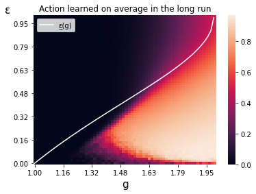
Action learned on average at triplet $(g,\varepsilon,\varepsilon)$

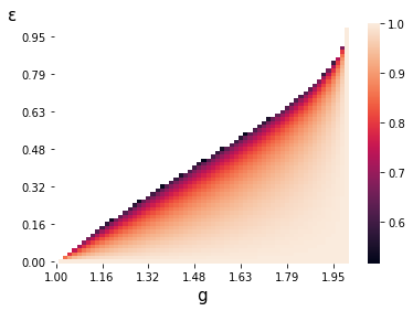
Theoretical time in $CC$ at the pseudo-equilibrium

Figure 1: Time spent in $\omega_{CC}$: simulations v.s. theory

The difference observed between Fig. 1’s left panel and the theoretical time spent in $CC$ at the pseudo-equilibrium (displayed in Fig. 1’s right panel) can be interpreted as the effect of the basin of attraction of the $\omega_{DD}$-equilibrium v.s. the one of the pseudo-equilibrium. The effect of $\varepsilon$ and $g$ on it is seemingly important.

6.3 Measuring $\lambda(\mathcal{B}(\varepsilon_{A},\varepsilon_{B},g))$

In this section, our objective is to find a method to measure the size of the basin of attraction of spontaneous coupling in order to distinguish its effect on $\tau^{g}_{CC}$ from the length and frequency of periods spent in $\omega_{CC}$. For this purpose, we perform two distinct clustering tasks using a simple K-means algorithm [30, 31] with two clusters (K=2). In the first task, we measure $\tau^{g}_{CC}$ by counting the number of periods algorithms spend in $\omega_{CC}$ once they have reached their limiting behavior, and then we classify triplets of parameters into two categories, either allowing for spontaneous coupling or not, using the $\tau^{g}_{CC}$ as a feature. The algorithm successfully identifies one cluster with low values of $\tau^{g}_{CC}$ and another with higher values, the second being the triplets of parameters allowing for spontaneous coupling. Then, for triplets of parameters for which spontaneous coupling is detected, we simulate $k$ (either $k=100$ or $k=1000$ depending on the computational intensity of the experiments) runs of our Q-learning algorithms, get the limiting Q-values and use them in a similar clustering task. More information about the clustering tasks performed is available in Appendix. Once the clusters are identified, we count how many of the runs ended up in each cluster to get a measure of $\lambda(\mathcal{B}(\varepsilon_{A},\varepsilon_{B},g))$. We show the outcome of our measurements in Fig. 2.

Our results indicate that, for a given $g$, spontaneous coupling appears for moderate values of $\varepsilon_{A}$ and $\varepsilon_{B}$. In line with Banchio and Mantegazza’s results, this region gets bigger when $g$ increases, covering $0\%$ of the plane $(\varepsilon_{A},\varepsilon_{B})\in[0,1]$ in the case $g=1$ up to $80\%$ of it. Interestingly, no spontaneous coupling is detected at all for values of $g$ below $1.4$, which contradicts Banchio and Mantegazza’s theoretical result. This might be due to our detection method, but in any case, our simulations indicate that spontaneous coupling is reached with negligible probability ($\lambda(\mathcal{B}(\varepsilon_{A},\varepsilon_{B},g))\approx 0$) when $g$ is too low. Also, we note that within the existence region, the effect of $(\varepsilon_{A},\varepsilon_{B})$ is relatively small. Particularly when $g$ is high, most of the parameters allowing for spontaneous coupling feature a negligible probability to end up in the $DD$ equilibrium ($\lambda(\mathcal{B}(\varepsilon_{A},\varepsilon_{B},g))\approx 1$). Finally, we note that asymmetry per se is detrimental to spontaneous coupling as $\lambda(\mathcal{B}(\varepsilon_{A},\varepsilon_{B},g))$ is typically lower when $\varepsilon_{A}$ and $\varepsilon_{B}$ are very different. Intuitively, when this is the case, for example if $\varepsilon_{A}>>\varepsilon_{B}$, under spontaneous coupling, $A$ often defects in the $\omega_{CC}$ periods causing Q-values of $B$ for action $C$ not to increase enough. For spontaneous coupling to be sustained in this case, more favorable (i.e. higher) initial conditions for $Q_{C}$ should be chosen, thus reducing $\lambda(\mathcal{B}(\varepsilon_{A},\varepsilon_{B},g))$.

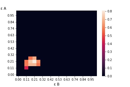
$g=1.42$

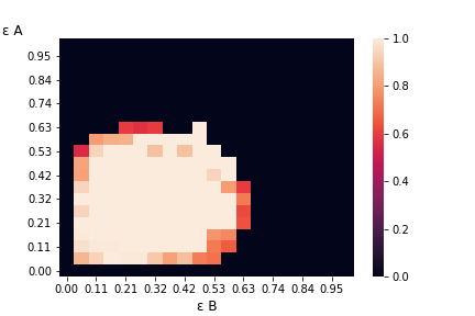
$g=1.68$

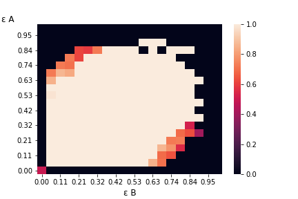
$g=1.84$

Figure 2: $\lambda(\mathcal{B}(\varepsilon_{A},\varepsilon_{B},g))$ on heatmaps for different values of $g$

6.4 Time spent in each region under spontaneous coupling

As we explained, under spontaneous coupling, algorithms alternate between phases of mutual cooperation, mutual defection and asymmetric behavior. In this section, we aim at measuring those times as functions of $\varepsilon_{A},\varepsilon_{B}$ and look at the specific case $g=1.7$. In order to do so, for one couple $(\varepsilon_{A},\varepsilon_{B})$ we simulate the process $k=100$ times for $=100000$ periods each and save the Q-values for the last $1000$ periods. We then are able to get the frequency with which a transition from a region to another happens, as if the process were markovian with respect to its being in $\omega_{CC},\omega_{CD},\omega_{DC}$ or $\omega_{DD}$. In particular, we get the probability with which the system remains in $\omega_{CC}$ (i.e. the probability of a $\omega_{CC}$ to $\omega_{CC}$ transition conditional on being in $\omega_{CC}$), the probability with which it remains in $\omega_{DC}$ and the probability of a $\omega_{CC}$ to $\omega_{CD}$ transition to happen conditional on a transition from $\omega_{CC}$ to $\omega_{CD}\cup\omega_{DC}$ to happen. The first two give a sense of how long the $\omega_{CC}$ and $\omega_{CD}$ phases are, while the third one indicates with which frequency an asymmetric transition is beneficial to player $B$. Those measures are represented using heatmaps in Fig. 3.

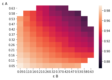
$\omega_{CC}\rightarrow\omega_{CC}$

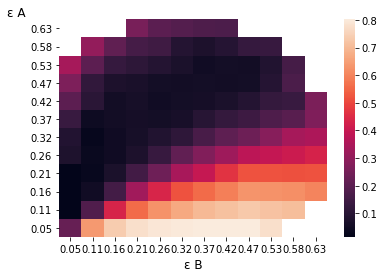
$\omega_{CD}\rightarrow\omega_{CD}$

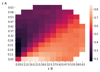
$\omega_{CC}\rightarrow\omega_{CD}|\omega_{CC}\rightarrow\omega_{CD}\cup\omega_{DC}$

Figure 3: Transitions probabilities for $g=1.7$

Results indicate that the length of cooperative periods is monotonic with each $\varepsilon$: an increase in one’s own exploration parameter is always harmful to cooperation in the sense that the system will spend less time in $\omega_{CC}$ and more time in either $\omega_{DD}$ or in asymmetric regions. This is coherent with the intuition we gave to spontaneous coupling: when $\varepsilon$ is higher, the Q-value for $D$ is updated more often in the $\omega_{CC}$ phases, causing it to increase faster and eventually to get above that of $C$ quicker. The transition from $\omega_{CD}$ to $\omega_{CD}$ (second heatmap of Fig. 3) gives us the following information. When $\varepsilon_{A}>\varepsilon_{B}$, the time spent in $\omega_{CD}$ is quite short and almost constant, whereas in the other part of the heatmap, it is longer, increasing in $\varepsilon_{B}$ and decreasing in $\varepsilon_{A}$. To understand this fact, one should see that when the system is in $\omega_{CD}$, it was most probably previously in $\omega_{CC}$. The transition from $\omega_{CC}$ to $\omega_{CD}$ happened as $B$ was quicker to realize that $D$ yields a higher payoff. Until $A$ realizes this fact too, the system remains in $\omega_{CD}$. Thus, in the bottom right part of the heatmap, when $\varepsilon_{B}$ increases, $B$ gets further ahead of $A$ in realizing action $D$ is dominant, while when $\varepsilon_{A}$ increases, $A$ is quicker to catch up with $B$. When $\varepsilon_{A}>\varepsilon_{B}$, time spent in $\omega_{CD}$ is small and due to randomization so that it is weakly affected by exploration parameters. Finally, the third heatmap of figure 3 generally confirms the interpretation given for the second one, though we note a non-linearity in the bottom right part which we could not explain so far. Surprisingly, for a given value of $\varepsilon_{A}$ there seems to be an intermediate value of $\varepsilon_{B}$ that gets the system in $\omega_{CD}$ rather than in $\omega_{DC}$ with highest probability.

6.5 Vizualizing $\tau^{g}_{X,Y}$

More broadly, time spent in each region can be measured following a similar method as previously and yields results aggregating both the effect of $\lambda(\mathcal{B}(\varepsilon_{A},\varepsilon_{B},g))$ and of the length of periods inside specific regions. We represent the outcome in Fig. 4. The time spent in $\omega_{CC}$ is non-monotonic, generally it tends to be higher when exploration parameters are low and symmetric. We do not really observe this non-monotonicity for $\omega_{DD}$, except at the boundaries of the existence region, which corresponds to the effect of exploration policies on the basin of attraction of spontaneous coupling we discussed in section 6.3. Finally, we point that time spent in symmetric regions (either $\omega_{CD}$ or $\omega_{DC}$) increases with the difference between $\varepsilon_{A}$ and $\varepsilon_{B}$. Those three observations together seem to indicate that when the player holding the highest exploration parameter decides to unilaterally increase it, the time taken from $\tau^{g}_{CC}$ is spent in an asymmetric region rather than in $\tau^{g}_{DD}$. Thus the effect of one player’s exploration parameter on $\tau^{g}_{CC}$ is non-monotonic, and $\varepsilon$s should be equal in order for $\tau^{g}_{CC}$ to be maximized.

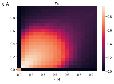
$\tau^{g}_{CC}$

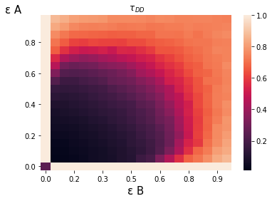
$\tau^{g}_{DD}$

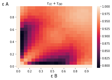
$\tau^{g}_{CC}+\tau^{g}_{DD}$

Figure 4: $\tau^{g}_{X,Y}$ for $g=1.7$

7 General equilibria of $G(g)$

In this section we turn our attention to $G(g)$ and its equilibria. We have proven in section 5 that $(0,0)$ is always a Nash equilibrium, now we aim at numerically finding other equilibria by using our simulations and see how they behave as a function of $g$.

7.1 Best response functions: shapes and interpretation

As a first step into looking what happens in equilibrium, we generate best response functions and look at their shapes.

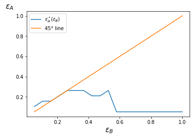
$g=1.53$

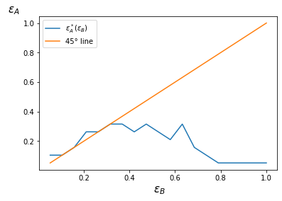
$g=1.63$

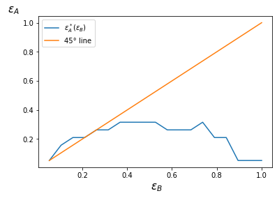
$g=1.73$

Figure 5: Best response functions for different values of $g$

Figure 5 displays the shape of best response functions for three different values of $g$. Although the result is pretty noisy (due to noise in the payoff matrix generation method), we note that the curves all share a common pattern: there is a first phase during which it is increasing and somehow follows the $45$° line, followed by a decreasing phase which ends up in it being flat and equal to $0$. The last portion has a very straightforward interpretation: when $\varepsilon_{B}$ is big, the chance to end up in $\omega_{DD}$ is high no matter what. Thus, a best response for $A$ is to set his exploration policy to $0$: otherwise, $A$ will be playing $C$ with some probability, while $C$ is dominated by $D$. Note that the length of the flat part is decreasing in $g$: this also has a straightforward explanation. We have proven already that the best response to $\varepsilon_{B}=1$ is $\varepsilon_{A}=0$. The higher $g$, the easier it is to sustain cooperative outcomes even by having $\varepsilon_{B}$ quite high.

Conditional on being in a cooperative pseudo-equilibrium with sufficient time spent in the cooperative part of space, exploration has the advantage of exploiting the other’s cooperation. Indeed, when in $\omega_{CC}$, raising one’s exploration level allows to play $D$ more often during this period of time and thus to make higher payoff. However, this is payoff reducing when in $\omega_{DD}$: in this case the situation is reversed, as adopting high exploration causes to play $C$ more often while the other player plays $D$. On top of this, we have seen in section 6.5 that increasing one’s exploration when it’s higher than the other player’s has the effect of reducing $\tau^{g}_{CC}$ and to increase $\tau^{g}_{DD}$. This explains why the best response functions are generally close to the $45$° line when their curve is located above the latter. If agents were to increase their exploration policy too much, they would simply break the spontaneous coupling. We can consider the most extreme case to illustrate. $A$ would like to have exploration level set at $1$ if he had the guarantee that players will remain in the cooperative pseudo-equilibrium, though we have proven already that this would cause the system to go to $\omega_{DD}$ for sure. Thus, if $A$ chooses $\varepsilon_{A}=1$, he is sure to drive the system in $\omega_{DD}$ and get into a bad position (a high exploration level in $\omega_{DD}$). When $\varepsilon_{B}$ increases, for a given $\varepsilon_{A}$, the risk of breaking the pseudo-equilibrium increases, so that the best response functions are eventually flat for large $\varepsilon_{B}$. Note how, when $g$ increases, the flat part of the curve begins for higher values of $\varepsilon_{B}$, which is clearly related to higher $g$ allowing for spontaneous coupling for larger exploration policies.

An additional mechanism needs to be added to get an intuition of the increasing part of the best response functions. We have seen that when $\varepsilon_{B}$ is above $\varepsilon_{A}$, increasing $\varepsilon_{A}$ has a two-fold effect. First, it increases the time spent in $\omega_{CC}$ which is beneficial to $A$, especially since she is increasing her exploration policy. Second, it allows to reduce the time spent in $\omega_{CD}$ and to eventually (when $\varepsilon_{A}$ gets higher than $\varepsilon_{B}$) increase the time spent in $\omega_{DC}$. This feature is of clear strategic interest, as during the time spent in this region, he will be playing $D$ quite often while $B$ will be playing $C$, allowing to collect higher payoff by exploiting the other’s cooperation. Now, starting from $\omega_{CC}$, agents will most likely go to $\omega_{CD}$ or $\omega_{DC}$, the quickest, i.e. generally the one with the highest exploration policy, wins the race and gets into a favorable position. As we have seen with our simulation results in Section 6.4 though, there is a non-linearity making this mechanism non-trivial.

8 Equilibrium results

8.1 Method

The game we consider is obviously symmetric, so that, given we have simulated the best response functions it is enough to look for the intersection of their curve with their symmetric with respect to the $45$° degree line. By this method we are able to get, for each $g$, Pareto optimal profiles as well as symmetric and non symmetric Nash equilibria. Of course, because the generation of the payoff matrix is noisy in essence, the equilibria we get will be noisy as well, so that we seek to interpret the general pattern of equilibria that may arise from this process.

Figure 6: All equilibria displayed on the learned-action heatmap

Figure 6 shows the result of the identification of equilibria for different values of $g$. It displays Pareto optimal profiles, as well as equilibria distinguished by whether they are symmetric or not. They are all plotted on the previously studied heatmap in order to know whether the equilibrium is in a region allowing for cooperation or not.

This way of plotting equilibria requires plotting an two dimensional profile on a one dimensional axis. For symmetric equilibria, this doesn’t impose any difficulty. When it comes to asymetric equilibria, we plot both $\varepsilon_{A}$ and $\varepsilon_{B}$ and recall that if $(\varepsilon_{A},\varepsilon_{B})$ is a Nash equilibrium, then $(\varepsilon_{B},\varepsilon_{A})$ is also, by symmetry of the game. We use the same method for Pareto optimal profiles, so that when two profiles seemingly appear, it needs to be read as only one asymetric profile.

8.2 Nash equilibria

It is clear from the figure that Nash equilibria are, for a vast majority, symmetric, and that asymmetric equilibria are such that the exploration policies are close to each other. Thus, we interpret this feature as the equilibria being generally symmetric but some of them appear asymmetric because of noise. When it comes to Pareto optimal profiles, once again, it is clear from the picture that they are mostly symmetric, and asymmetric profiles have close exploration policies. We see that $\varepsilon_{A}=\varepsilon_{B}=0$ often comes out as an equilibrium, in conformity to our previous theoretical result, though many other equilibria exists, in particular when $g$ is high enough. When a symmetric profile allowing for a good level of exploration exists (i.e. when some cells of the heatmap have a light color) it is notable that equilibria tend to be located inside the region, which confirms the existence of highly cooperative Nash equilibria under competition over parameters, in line with our last theoretical result.

When $g$ is small, we note that the only Nash equilibrium is the $(0,0)$ one. This relates to the bassin of attraction of spontaneous coupling being negligible for $g$ too small. In this case, the best response functions are constantly equal to $0$ so that the only equilibrium is clearly $(0,0)$. Then, equilibria have a striking bell-shaped distribution with $g$. In order to get an intuition for this, we spot the following tradeoff. When $g$ is low, exploration is very costly as it is very likely to break the pseudo-equilibrium. As $g$ increases, agents thus have more latitude in choosing a high exploration policy. However, the attractiveness of exploration tends to decrease with $g$. Indeed, exploring in the case of a pseudo-equilibrium enables players to play $D$ instead of $C$. Thus, when the opponent is playing $C$, instead of making $2g$, a player will be getting $2+g$, and when the opponent plays $D$, he gets $2$ instead of $g$: the net benefit of playing $D$ over $C$ is thus alway $2-g$, so that the incentive to deviate from mutual cooperation tends to decrease. Because of this, as $g$ increases, there is a tendency to prefer cooperative outcomes. Those conflicting tendencies are a beginning for an explanation of the bell shape we observe, our guess being that the latitude given to players in choosing higher exploration policy is a concave function of $g$ which becomes dominated by the other (linear) effect on incentives to deviate.

8.3 Pareto optimal profiles

First thing to note when it comes to Pareto optimal profiles is that they are all symmetric, which is a consequence of symmetric profiles minimizing the time spent in $\omega_{CD}\cup\omega_{DC}$, which are harmful in term of joint payoff, and of $\tau_{CC}$ being increased when the highest exploration parameter is reduced. Put differently, for any couple of asymmetric exploration parameters such that $\varepsilon_{A}>\varepsilon_{B}$, by considering the profile $(\varepsilon_{B},\varepsilon_{B})$ we reduce the time spent in $\omega_{CD}\cup\omega_{DC}$, increase the time spent in $\omega_{CC}$ and reduce the one spent in $\omega_{DD}$ which intuitively increases the joint output. The distribution of Pareto optimal profiles has a nice and easy interpretation. To maximize social surplus, there is a trade-off. Increasing the exploration level gives a benefit for the periods in which $D$ is held as a preferred action, and is costly in the other case. On top of this, it is socially better to choose low exploration policies in order to maximize time spent in $\omega_{CC}$. As $g$ increases, for a given profile, the time spent in $\omega_{DD}$ tends to decrease, and thus the social benefit to choose a high exploration policy decreases. This explains the generally decreasing shape of the distribution of Pareto optimal profiles. When $g$ is too low, the time spent in $\omega_{CC}$ is virtually $0$ no matter the exploration policy, so that the socially optimal profile is clearly to choose $\varepsilon_{A}=\varepsilon_{B}=1$. Note also how Pareto optima get steady for high values of $g$, yet clearly above $0$. This can be related to minimal exploration being required in order to maximize the probability of reaching spontaneous coupling as our results of Section 6.3 have shown. Also, in the second part of the distribution (for values of $g$ in which some time is actually spent in $\omega_{CC}$), we note that Pareto optimal values of exploration are typically lower than equilibrium ones, i.e. agents tend to over-explore. This reveals how there is an incentive to unilaterally increase the exploration level when spontaneous coupling appears with a high enough probability so as to often play $D$ when the other is playing $C$ in order to get $2+g$ rather than $2g$. Our guess is that this difference between Pareto optimal profiles and Nash equilibria is limited by the effect player’s individual exploration parameter have on the time spent in $\tau_{CC}$. If this is the case, it should intuitively be increased when there are more players involved.

9 Conclusion

We have shown that the mechanism responsible for algorithmic collusion persists by allowing different exploration policies. More than that, we have provided evidence that, in equilibrium, there is collusion. The essential trade-off to retain from our analysis is that there is an incentive to increase one’s exploration policy in order to exploit the other players during the time spent in $\omega_{CC}$, however this comes at the risk of breaking the spontaneous coupling, which is detrimental to players. As players are able to guarantee themselves the best possible situation in a non-cooperative outcome by setting their exploration level equal to zero, in equilibrium, there is no room for situations including coupling that would be very detrimental to one of the players. This however gives insight on the difference between equilibrium profiles and Pareto ones, indicating that competition between algorithms potentially decreases the degree of collusion. Further, our simulations shed light on more involved mechanisms regarding time spent in asymmetric regions: a player might want to raise his exploration level above the one of his opponent in order to benefit from time spent in positively asymmetric situation. By doing so, one’s algorithm realizes quicker than the other that $D$ is a dominant strategy and benefits from his opponent’s slowness. This however comes at the risk of transitioning too fast from $DD$ phases to a negatively asymmetric phase.

Our results call for further work. In particular, we chose to let exploration policies be different because they have a straightforward interpretation. A similar analysis could well be applied to the learning rate $\alpha$, which we left exogenously fixed. Same goes with the initial conditions, which could be regarded as parameters of the algorithms and thus chosen beforehand by players. In particular, we believe that further work on initial conditions is needed so as to better understand algorithmic interactions and to get stronger results. Also, our findings suggest that competition makes equilibrium exploration levels higher than Pareto ones, so that in a sense, collusion is weakened by competition between algorithms. An interesting question could be to model what happens when more than two Q-learning interact. Our intuition is that, by decreasing the impact individual exploration has on the system as a whole, its cost decreases while it remains beneficial, so that possibly collusion disappears when the number of agents is large.

10 Appendix

10.1 Detection of spontaneous coupling: method

In order to detect spontaneous coupling and measure its basin of attraction, we rely on the position of Q-values in the four-dimensional space $(Q^{A}_{C},Q^{A}_{D},Q^{B}_{C},Q^{B}_{D})$ after a large enough number of periods. In Fig. 7 we plot the projection of the position of the system on a plane for $K=1000$ different initial conditions uniformly drawn at random in $\mathbb{I}$ : a red dot corresponds to the position of player’s $B$ Q-values for one initial condition, while a blue dot corresponds to that of player $A$. The black lines correspond to values $\frac{2}{1-\gamma}$ and $\frac{2g}{1-\gamma}$, for which $Q_{C}$ can be above $Q_{D}$.On the first panel ($g=1.7,\varepsilon_{A}=\varepsilon_{B}=0.1$), we clearly see that two clusters exist. The one on the top right part of the figure corresponds to the spontaneous coupling being reached, while the second corresponds to the system reaching $\tilde{\mathbb{Q}}^{\text{eq}}_{DD}$. The simple idea behind our measuring the basin of attraction of spontaneous coupling relies on automatically detecting those clusters and measuring their sizes. In order to do so, we use a simple K-means algorithm with $K=2$, let it detect the clusters and label the points accordingly.

K-means is a well-known simple algorithm to perform unsupervised learning. Given a set of points in a space, it aims at minimizing an inertia metric (which is the average distance of points to the center of their clusters) by assigning observation to clusters in a good way. K-means, even though known to perform good for simple task, is still a heuristic method in the sense that it does not necessarily produce the best clustering. In our case, since the task is pretty simple, we do not look more advanced methods of clustering. In essence, K-means takes as input a list of observations, in our case a list of $4$-dimensional points, and a number of clusters (in our case $K=2$), and gives the centers of the identified clusters as well as the cluster to which each observation belongs, which enables to compute the inertia metric of the achieved clustering. It proceeds as follows: first, it chooses randomly $K$ observations to behave as clusters and produces the associated Voronoï diagram (i.e. assigns each observation to the cluster with nearest center). Then, it updates the centers of the clusters given the new partition of observations and repeats the operation. The process stops whenever the clusters’ centers do not move anymore.

It is important to note that K-means requires the number of clusters to be set in advance, and thus cannot by itself find the optimal number of clusters to perform its task. In our case, this causes issues for two cases. The first case is the one in which spontaneous coupling does not exist and thus only one cluster can be found (corresponding to $\tilde{\mathbb{Q}}^{\text{eq}}_{DD}$). The second panel of Fig. 7 shows an example where this happens. The second case is the one in which convergence to $\tilde{\mathbb{Q}}^{\text{eq}}_{DD}$ do not show up in our experiments, so that in this case too, only one cluster appears (see the third panel of Fig. 7 for an example). If we were to try and measure the size of the basin of attraction of spontaneous coupling in those cases, the K-means algorithm would identify two clusters of equal size and thus give us a wrong measure. In order to circumvent this difficulty, we perform two additional clustering tasks using K-means algorithms with $K=2$. The first one aims at identifying the parameters which allows for spontaneous coupling. For this purpose, we use the time spent in $\omega_{CC}$ as a feature and run a K-means algorithm in one dimension. Since we know the results should display two clusters (i.e. allowing for spontaneous coupling or not allowing for spontaneous coupling) there is no problem in fixing beforehand the number of clusters to be $2$. Doing so, we successfully identify parameters allowing for spontaneous coupling, and for those who don’t, we fix the measure of the basin to be $0$. We then proceed to perform the clustering task we previously described, and get two features out of it. First, we get the inertia metric associated to this task’s outcome as well as the inertia metric associated to the trivial task with $K=1$ and compute their difference. Second, we get the distance between the identified clusters’ centers. We use those two features to perform yet another K-means clustering with $K=2$ on the parameters allowing for spontaneous coupling. The idea is the following: when the distance between clusters’ centers and the difference in the inertia metric are high, this reveals that two clusters exist in the $4$-dimensional space, while when they are small, only one cluster should be considered. For parameters belonging to this category, we fix the size of the basin of attraction to $1$ and consider the $\tilde{\mathbb{Q}}^{\text{eq}}_{DD}$ equilibrium to be reached for a negligible fraction of initial conditions.

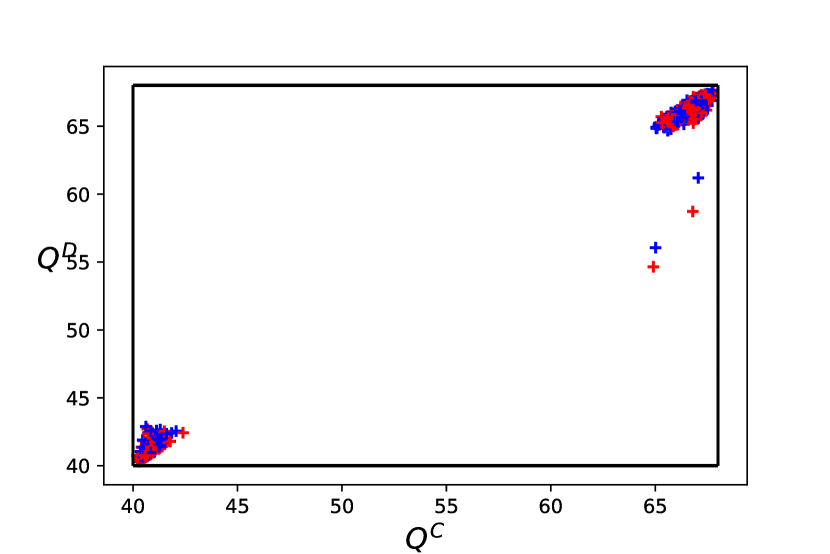
$g=1.7,\varepsilon_{A}=\varepsilon_{B}=0.1$

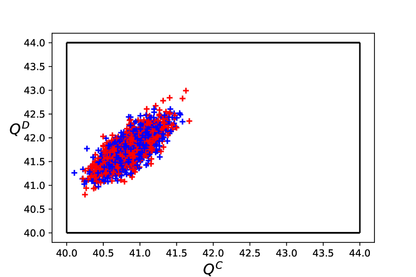
$g=1.1,\varepsilon_{A}=\varepsilon_{B}=0.3$

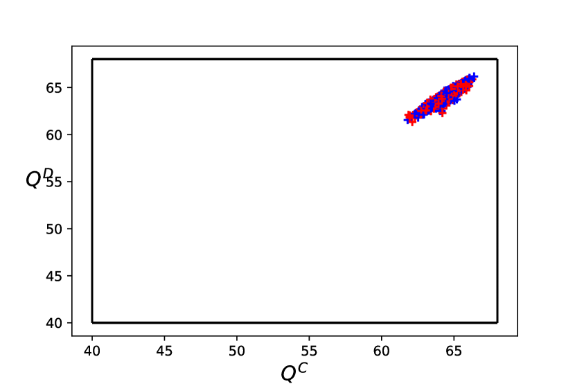
$g=1.7,\varepsilon_{A}=\varepsilon_{B}=0.3$

Figure 7: Projection on a plane of the position of the system in the $4$ dimensional space

10.2 Proof of mathematical results

Proposition 1.

Assume $\varepsilon_{A},\varepsilon_{B}>0$. Then with probability $1$ there exists $t$ such that:

$$\forall i\in\{A,B\},\forall X\in\{C,D\},Q_{i}^{X}(t)\in[\frac{\tilde{\pi}^{P}_{X,D}}{1-\gamma},\frac{\tilde{\pi}^{P}_{X,C}}{1-\gamma}]$$ (20)

Proof.

When action $X$ is chosen by player $i$ at time $t$, its Q-value is updated as follows:

$$Q_{i}^{X}(t+1)=(1-\alpha)Q_{i}^{k}(t)+\alpha\Big{[}\gamma\max_{X^{\prime}\in\{C,D\}}Q_{i}^{X^{\prime}}(t)+r_{X}^{i}(t)\Big{]},$$ (21)

where $r_{X}^{i}(t)$ is the (stochastic) reward received by player $i$ at $t$. This reward has two possible values: $\tilde{\pi}^{i}_{X,D}$ and $\tilde{\pi}^{i}_{X,C}$, which are such that $\tilde{\pi}^{i}_{X,C}\geq\tilde{\pi}^{i}_{X,D}$. One can rewrite the above equation and get:

$$\Delta(Q_{i}^{X})(t)\equiv Q_{i}^{X}(t+1)-Q_{i}^{X}(t)=\alpha\Big{[}r_{X}^{i}(t)-\big{(}Q_{i}^{X}(t)-\gamma\max_{X^{\prime}}Q_{i}^{X^{\prime}}(t)\big{)}\Big{]},$$ (22)

so that there are two cases:

$$\frac{1}{\alpha}\Delta(Q_{i}^{X})(t)=\left\{\begin{array}[]{ll}r_{X}^{i}(t)-\Big{(}Q_{i}^{X}(t)-\gamma\max_{X^{\prime}}Q_{i}^{X^{\prime}}(t)\Big{)}\text{ if }X\neq\arg\max_{X^{\prime}}Q_{i}^{X^{\prime}}(t).\\ r_{X}^{i}(t)-(1-\gamma)Q_{i}^{X}(t)\text{ if }X=\arg\max_{X^{\prime}}Q_{i}^{X^{\prime}}(t).\end{array}\right.$$ (23)

Note that in both cases:

$$\frac{1}{\alpha}\Delta(Q_{i}^{X})(t)\geq r_{X}^{i}(t)-(1-\gamma)Q_{i}^{X}(t)$$ (24)

So that if $Q_{i}^{X}(t)<\frac{\tilde{\pi}^{i}_{X,D}}{1-\gamma}$:

$$\frac{1}{\alpha}\Delta(Q_{i}^{X})(t)\geq\tilde{\pi}^{i}_{X,D}-(1-\gamma)\frac{\tilde{\pi}^{i}_{X,D}}{1-\gamma}=0.$$ (25)

Thus, if $Q_{i}^{X}(t)$ is below $\frac{\tilde{\pi}^{i}_{X,D}}{1-\gamma}$, it grows. Now, assume for some $t$, $Q_{i}^{X}(t)\geq\frac{\tilde{\pi}^{P}_{X,D}}{1-\gamma}$, then:

$$\begin{split}Q_{i}^{X}(t+1)&=(1-\alpha)Q_{i}^{X}(t)+\alpha\Big{[}\gamma\max_{X^{\prime}}Q_{i}^{X^{\prime}}(t)+r_{X}^{i}(t)\Big{]}\\ &\geq(1-\alpha)\frac{\tilde{\pi}^{i}_{X,D}}{1-\gamma}+\alpha\Big{[}\gamma\frac{\tilde{\pi}^{i}_{X,D}}{1-\gamma}+\tilde{\pi}^{i}_{X,D}\Big{]}\geq\frac{\tilde{\pi}^{i}_{X,D}}{1-\gamma}.\end{split}$$ (26)

It is then clear that, with probability $1$, there exists $t^{*}$ such that for all $t>t^{*}$, for all $i\in\{A,B\}$ and for all $X\in\{C,D\}$, $Q_{i}^{X}\geq\frac{\tilde{\pi}^{i}_{X,D}}{1-\gamma}$.

Now assume that for some $X\in\{C,D\}$, $Q_{i}^{X}(t)>\frac{2+g}{1-\gamma}$. There are two cases:

• If $X^{*}=\arg\max_{X}^{\prime}Q_{i}^{X}(t)$ is chosen at $t$, then:

  $$\Delta(Q_{i}^{X^{*}})(t)=\alpha\Big{[}r_{X}^{i}(t)-(1-\gamma)Q_{i}^{X^{*}}\Big{]}<0,$$ (27)

  and for $X\neq X^{*}$, $Q_{i}^{X}$ is unchanged.

• If $X\neq\arg\max_{X}^{\prime}Q_{i}^{k}(t)$ is chosen at $t$, then:

  $$\begin{split}Q_{i}^{X}(t+1)&=(1-\alpha)Q_{i}^{X}(t)+\alpha\Big{[}\gamma\max_{X^{\prime}}Q_{i}^{X^{\prime}}(t)+\tilde{\pi}_{X}^{i}(t)\Big{]}\\ &\leq(1-\alpha)\max_{X^{\prime}}Q_{i}^{X}(t)+\alpha\Big{[}\gamma\max_{X^{\prime}}Q_{i}^{X^{\prime}}(t)+(1-\gamma)\max_{X^{\prime}}Q_{i}^{X^{\prime}}\Big{]}\\ &\leq\max_{X^{\prime}}Q_{i}^{X}(t).\end{split}$$ (28)

Thus, if one of the Q-values is above $\frac{2+g}{1-\gamma}$, the maximum of Q-values needs to decrease. Then if it is the case, for sure for some $t$ further in time $\max_{X^{\prime}}Q_{i}^{X^{\prime}}(t^{\prime})\leq\frac{2+g}{1-\gamma}$. For such $t^{\prime}$, for all $i,X$:

$$Q_{i}^{X}(t+1)\leq(1-\alpha)\frac{2+g}{1-\gamma}+\alpha(2+g)+\alpha\gamma\frac{2+g}{1-\gamma}=\frac{2+g}{1-\gamma}.$$ (29)

Then clearly, with probability $1$, there exists $t^{\prime*}$ such that for all $t>t^{\prime*}$, for all $i,X$, $Q_{i}^{X}\leq\frac{2+g}{1-\gamma}$.
Now, assume for some $i$, and for some $t>\max(\{t^{*},t_{1}^{*}\})$, $Q_{i}^{C}(t)\in]\frac{2g}{1-\gamma},\frac{2+g}{1-\gamma}]$. Consider a specific sequence of plays such that: $i$’s opponent always plays $D$, and $i$ always plays the action with highest Q-value. The probability of such sequence of plays of length $L$ is higher than $\Big{(}\frac{\epsilon_{j}}{2}(1-\epsilon_{i})\Big{)}^{L}$. In this case, in each step, the Q-value of the updated action decreases at least by $\alpha g$ if $C$ has the highest Q-value, and at least by $2\alpha(g-1)$ if $D$ has the highest Q-value. Thus, any such sequence of length

$$L=\Big{\lceil}\frac{2}{1-\gamma}\frac{1}{2\alpha(g-1)}\Big{\rceil}$$ (30)

is guaranteed to drive $Q_{i}^{C}$ below $\frac{2g}{1-\gamma}$. Reiterating this process with the other player in the case he has a Q-value for $C$ higher than $\frac{2g}{1-\gamma}$ yields the same result. Since this happens with strictly positive probability, we know that with probability $1$, the Q values will be in the desired interval at some point in time. ∎

Proposition 2.

$\forall(\varepsilon_{A},\varepsilon_{B},g)\in[0,1]\times[0,1]\times[1,2]$, there exists a steady state $\tilde{\mathbb{Q}}^{\text{eq}}_{DD}$ of the continuous time equivalent that lies in $\omega_{DD}$. No other steady-state exists.

Proof.

This result is simply obtained by setting the flow of the continuous time equivalent in $\omega_{DD}$ to $(0,0,0,0)$. For $(X,Y)\neq(D,D)$ non-existence is obtained by setting the flow in $\omega_{X,Y}$ to $(0,0,0,0)$ and observing the solution does not lie in $\omega_{X,Y}$. ∎

Proposition 3.

For any $g\in[0,1]$, if $\varepsilon_{A}=1$ or $\varepsilon_{B}=1$, $(\varepsilon_{A},\varepsilon_{B},g)$ does not allow for spontaneous coupling.

Proof.

In this case, for any $(X,Y)\in\{C,D\}^{2}$, the dynamics within $\omega_{X,Y}$ solve:

$$\left\{\begin{array}[]{ll}\dot{Q}_{A}^{X}(t)=\frac{\alpha}{2}\Big{[}\hat{\pi}_{X,Y}-(1-\gamma)Q_{A}^{X}(t)\Big{]}\\ \dot{Q}_{A}^{-X}(t)=\frac{\alpha}{2}\Big{[}\hat{\pi}_{-X,Y}+\gamma Q_{A}^{X}(t)-Q_{A}^{-X}(t)\Big{]}.\end{array}\right.$$ (31)

Taking the difference between the two equations allows us to get a differential equation for $\Delta(Q_{A}^{X})(t)$:

$$\dot{\Delta(Q_{A}^{X})}(t)+\frac{\alpha}{2}\Delta(Q_{A}^{X})(t)=\frac{\alpha}{2}\Big{(}\hat{\pi}_{X,Y}-\hat{\pi}_{-X,Y}\Big{)}.$$ (32)

This equation has a simple solution of the form:

$$\Delta(Q_{A}^{X})(t)=K_{0}\exp(-\alpha t)+\Big{(}\hat{\pi}_{X,Y}-\hat{\pi}_{-X,Y}\Big{)},$$ (33)

so that $\Delta(Q_{A}^{X})$ is monotonic and:

$$\left\{\begin{array}[]{ll}\Delta({Q}_{A}^{X})(0)\geq 0\text{ by definition }\\ \lim_{+\infty}\Delta({Q}_{A}^{X})(t)=\hat{\pi}_{X,Y}-\hat{\pi}_{-X,Y}.\end{array}\right.$$ (34)

Since $\hat{\pi}_{X,Y}-\hat{\pi}_{-X,Y}>0$ when $X=D$ and $\hat{\pi}_{X,Y}-\hat{\pi}_{-X,Y}<0$ when $X=C$, it is clear that whenever player A enters $D$ it remains in $D$, and eventually exits $C$ to $D$ when it is in $C$. Thus, no matter the initial condition:

$$\exists t^{*}\text{ s.t. }\forall t>t^{*},Q_{A}^{D}(t)>Q_{A}^{C}(t).$$ (35)

Now, we can focus on the Q values of player $B$, fixing the behavior of $A$ to be stationary. This defines a dynamic system on its own, characterized by the piece-wise linear dynamics of player B’s Q values. We proceed by contradiction, assuming that there is a pseudo equilibrium for this system. The linear dynamics in each continuity domain follow:

$$\vec{F}_{DC}^{B}=\begin{pmatrix}\alpha(1-\frac{\varepsilon_{B}}{2})\Big{[}\frac{g}{2}+g+\gamma Q_{B}^{D}(t)-Q_{B}^{C}(t)\Big{]}\\ \alpha\frac{\varepsilon_{B}}{2}\Big{[}\frac{2+g}{2}+1-(1-\gamma)Q_{B}^{D}(t)\Big{]}\end{pmatrix},$$ (36)

$$\vec{F}_{DD}^{B}=\begin{pmatrix}\alpha\frac{\varepsilon_{B}}{2}\Big{[}\frac{g}{2}+g-(1-\gamma)Q_{B}^{C}(t)\Big{]}\\ \alpha\frac{\varepsilon_{B}}{2}\Big{[}\frac{2+g}{2}+1+\gamma Q_{B}^{C}(t)-Q_{B}^{D}(t)\Big{]}\end{pmatrix}.$$ (37)

Let $\vec{N}=\begin{pmatrix}1\\ -1\end{pmatrix}$ the normal vector to $A=\{\begin{pmatrix}x\\ x\end{pmatrix},x\in\mathbb{R}\}$. Under our hypothesis, there exists $\tau^{*}$ such that:

$$\tau^{*}\vec{F}_{DC}^{B}|_{Q_{B}^{D}=Q_{B}^{C}}+(1-\tau^{*})\vec{F}_{DD}^{B}|_{Q_{B}^{D}=Q_{B}^{C}}=0,$$ (38)

and

$$\tau^{*}F_{DC}^{B}|_{Q_{B}^{D}=Q_{B}^{C}}+(1-\tau^{*})F_{DD}|_{Q_{B}^{D}=Q_{B}^{C}}^{B}=\vec{0}.$$ (39)

Solving the first equation for $\tau^{*}$ we get

$$\tau^{*}=\frac{2Q_{B}(1-\gamma)(1-\varepsilon_{B})+2\varepsilon_{B}(g+1)-(g+4)}{4(1-\varepsilon_{B})\Big{(}(1-\gamma)Q_{B}-(g+1)\Big{)}}$$ (40)

which we substitute in the second and get:

$$\frac{\alpha(3g-2(1-\gamma)Q_{B})(4+g-2(1-\gamma)Q_{B})}{8(1+g-(1-\gamma)Q_{B})}\begin{pmatrix}1\\ 1\end{pmatrix}=\vec{0},$$ (41)

which has two solutions:

$$Q_{B}=\frac{3g}{2(1-\gamma)}\text{ or }Q_{B}=\frac{4+g}{2(1-\gamma)}.$$ (42)

This gives two possibilities for $\tau^{*}$:

$$\tau^{*}=\frac{2-\varepsilon_{B}}{2(1-\varepsilon_{B})}>1\text{ or }-\frac{\varepsilon_{B}}{2(1-\varepsilon_{B})}<0.$$ (43)

This final line gives us a contradiction. ∎

Proposition 4.

For any $g\in[0,1]$, if $\varepsilon_{A}=0$ and $\varepsilon_{B}>0$, $(\varepsilon_{A},\varepsilon_{B},g)$ does not allow for spontaneous coupling.

Proof.

First we focus on the Q-values of player $A$. Since $\varepsilon_{A}=0$, in each period, $A$ only updates the highest Q-value. Thus, if $X$ is updated at $t$:

$$\Delta(Q_{A}^{X}(t)=\alpha\Big{[}r_{X}^{i}(t)-(1-\gamma)Q_{i}^{X}\Big{]}\geq 0\iff Q_{A}^{X}(t)\leq\frac{r_{X}^{i}(t)}{1-\gamma}.$$ (44)

As a consequence, when $Q_{A}^{X}(t)\in[\frac{\tilde{\pi}^{i}_{X,D}}{1-\gamma},\frac{\tilde{\pi}^{i}_{X,C}}{1-\gamma}]$, when updated, it grows when the reward received is high (i.e. when the opponent plays $C$) and it decreases when the reward received is low (i.e. when the opponent plays $D$). Note also that:

$$Q_{A}^{X}(t)\in[\frac{\tilde{\pi}^{i}_{X,D}}{1-\gamma},\frac{\tilde{\pi}^{i}_{X,C}}{1-\gamma}]\implies Q_{A}^{X}(t+1)\in[\frac{\tilde{\pi}^{i}_{X,D}}{1-\gamma},\frac{\tilde{\pi}^{i}_{X,C}}{1-\gamma}].$$ (45)

Let $Q_{A}^{C}(t)$ and $Q_{A}^{D}(t)$ in $\Big{[}\frac{2}{1-\gamma},\frac{2g}{1-\gamma}\Big{]}$. Any other situation can be proven to lead to this case. We prove that, with probability $1$, $Q_{A}^{C}$ goes under $\frac{2}{1-\gamma}$, in which case, for sure, $Q_{A}^{D}$ will remain higher than $Q_{A}^{C}$ onward.

Let a realization of rewards such that for all $t$, $Q_{A}^{C}\in[\frac{2g}{1-\gamma},\frac{2}{1-\gamma}]$. Consider a sequence of consecutive low rewards of length $L$. Along such a sequence, the Q values, when updated, decrease. More precisely:

$$\forall t\text{ s.t. }Q^{X}_{A}(t)>Q^{-X}_{A}(t),Q^{X}_{A}(t+1)=\Big{(}1-(1-\gamma)\alpha\Big{)}Q_{A}^{X}(t)+\alpha\underline{\pi}_{A}^{X}.$$ (46)

For $T^{X}$ a set of consecutive integers such that $\forall t\in T^{X},Q^{X}_{A}(t)>Q^{-X}_{A}(t)$, by denoting $T_{0}$ the first of them we get that:

$$\forall t\in T^{X},Q_{A}^{X}(t)=\Big{(}1-(1-\gamma)\alpha\Big{)}^{t}\Big{(}Q_{A}^{X}(T_{0})-\underline{\pi}^{X}_{A}\Big{)}+\frac{\underline{\pi}_{A}^{X}}{1-\gamma}.$$ (47)

We can also extract from the sequence $(Q_{A}^{X})_{t\in\mathbb{N}}$ the sequence $(Q_{A}^{X})_{t\in\bigcup T_{X}}$ and relabel time such that for all $k,t^{*}_{k}$ designates the $k$-th period of time at which action $X$ was updated. By the way, it is clear that by allowing $L$ large enough, we can get as many such periods of time as we want. Then one can note that:

$$\lim_{t^{*}_{C}\longrightarrow\infty}Q_{A}^{C}(t^{*}_{C})=\frac{g}{1-\gamma}<\frac{2}{1-\gamma}$$ (48)

so that there exists a finite $t_{k}^{*}$ such that $Q_{A}^{C}(t^{*}_{C})<\frac{2}{1-\gamma}$. Thus for any initial condition, by choosing $L$ large enough but finite, a sequence of $L$ consecutive low rewards leads to $Q_{A}^{C}$ exiting the interval. Note as well that the number of updates of $C$ necessary for this is biggest when $Q_{A}^{C}(0)$ is highest, thus there exists $L$ such that our previous result holds for any initial condition. Thus, whenever the Q values of $A$ lie in the interval $[\frac{2g}{1-\gamma},\frac{2}{1-\gamma}]$, if a large enough (but finite) sequence of low rewards happens, $Q_{C}^{A}$ will exit the interval. If we assume the $Q$ values remain inside for an infinite number of periods, then $Q_{C}^{A}$ exits with probability $1$. Finally, we conclude that, with probability $1$, there exists $t$ such that for any $t^{\prime}>t$, $Q_{A}^{C}(t)<\frac{2}{1-\gamma}$. By a similar reasoning than in Proposition 3, we get that there is no possible pseudo-equilibrium. ∎

Proposition 5.

For any $g$, $(0,0,g)$ allows for spontaneous coupling. More specifically for any initial condition in $\mathbb{I}$, there exists $t^{*}\in\mathbb{N}$ such that for all $t>t^{*},\mathbb{Q}(t)\in\omega_{CC}$ or $t^{*}\in\mathbb{N}$ such that for all $t>t^{*},\mathbb{Q}(t)\in\omega_{DD}$. Furthermore, $\tau^{g}_{CC}(0,0)\geq 4\Big{(}1-\frac{1}{g}\Big{)}^{4}\in[0,\frac{1}{4}]$.

Proof.

First, note that if for some $t$, $\mathbb{Q}(t)\in\omega_{CC}$, then for all subsequent $t^{\prime},\mathbb{Q}(t^{\prime})\in\omega_{CC}$. Then, for any initial condition starting the process in $\omega_{CC}$, the system will stay in $\omega_{C}C$. This happens with probability:

$$\mathbb{P}(\mathbb{Q}_{0}\in CC)=\mathbb{P}\Big{(}Q_{A}^{C}(0)<Q_{A}^{D}(0)\Big{)}\mathbb{P}\Big{(}Q_{B}^{C}(0)<Q_{B}^{D}(0)\Big{)}=\mathbb{P}\Big{(}Q_{A}^{C}(0)<Q_{A}^{D}(0)\Big{)}^{2},$$ (49)

where:

$$\mathbb{P}\Big{(}Q_{A}^{C}(0)<Q_{A}^{D}(0)\Big{)}=\int_{\frac{g}{1-\gamma}}^{\frac{2g}{1-\gamma}}\Big{(}\frac{1-\gamma}{g}\Big{)}^{2}\Big{(}x-\frac{2}{1-\gamma}\Big{)}dx=\frac{2}{g^{2}}(g-1)^{2}.$$ (50)

Now, assume that the system doesn’t end up in $\omega_{CC}$, then it must be the case that $\forall t,\mathbb{Q}(t)\in\omega_{DD}\cup\omega_{CD}\cup\omega_{DC}$. Further assume that $\forall t_{0},\exists t>t_{0}$ such that $\mathbb{Q}_{t}\in\omega_{CD}\cup\omega_{DC}$. Then, it is clear that for all $X\in\{A,B\}$, $\Big{(}Q_{C}^{X}(t)\Big{)}_{t\in\mathbb{N}}$ is a decreasing sequence, and strictly decreases each time $X$ holds $C$ as a preferred action. Also, it must be the case that there is $X$ such that $Q_{C}^{X}(t)>\frac{2}{1-\gamma}$, otherwise there is no way $Q_{C}^{X}(t)>Q_{D}^{X}(t)$. For each $t$ such that $Q_{C}^{X}(t)$ decreases we get:

$$Q_{C}^{X}(t+1)-Q_{C}^{X}(t)=\alpha\Big{(}g-(1-\gamma)Q_{C}^{X}(t)\Big{)}<\alpha(g-2).$$ (51)

By our hypothesis, it is clear that for both $A$ and $B$, $Q_{C}^{X}(t)<\frac{2}{1-\gamma}$ at some point, which is a contradiction. The first condition for allowing spontaneous coupling (i.e. the existence of an initial condition for which the continuous time equivalent does not end up in $\tilde{\mathbb{Q}}^{\text{eq}}_{DD})$ can be easily verified by taking an initial condition in $\omega_{CC}$ and checking the continuous time equivalent never leaves $\omega_{CC}$. ∎

Proposition 6.

For all $g\in[1,2]$, $(\varepsilon_{A}=0,\varepsilon_{B}=0)$ is a Nash equilibrium of $G(g)$. It is strict whenever $g>1$.

Proof.

Assume $\varepsilon_{B}=0$, then if $A$ chooses $\varepsilon_{A}>0$, by Proposition 4, the system converges to $\omega_{D}D$. Thus the payoff $A$ makes by choosing $\varepsilon_{A}>0$ is:

$$\pi_{A}(\varepsilon_{A},0)=2(1-\frac{\varepsilon_{A}}{2})+g\frac{\varepsilon_{A}}{2}<2$$ (52)

while the payoff $A$ makes when choosing $\varepsilon_{A}=0$ is:

$$2(1-\mathbb{P}(CC))+2g\mathbb{P}(CC)>2.$$ (53)

We deduce the result by symmetry of the game. ∎

Proposition 7.

For all $g\in]1,2[$, $\varepsilon=1$ is a dominated strategy in $G(g)$.

Proof.

Let $\varepsilon_{A}\in]0,1]$. If $\varepsilon_{B}=1$, then we know from Proposition 3 that $(\varepsilon_{A},\varepsilon_{B},g)$ does not allow for spontaneous coupling and thus $\tau_{DD}^{g}=1$. Thus player $B$ will receive payoff:

$$\Pi^{B}(\varepsilon_{A},1)=\Big{(}1-\frac{\varepsilon_{A}}{2}\Big{)}\frac{g+2}{2}+\frac{\varepsilon_{A}}{2}\frac{2g+2+g}{2}$$ (54)

whereas by playing $\varepsilon_{B}=0$ still $(\varepsilon_{A},\varepsilon_{B},g)$ does not allow for spontaneous coupling and he would get payoff:

$$\Pi^{B}(\varepsilon_{A},0)=\Big{(}1-\frac{\varepsilon_{A}}{2}\Big{)}.2+\frac{\varepsilon_{A}}{2}\Big{(}2+g\Big{)},$$ (55)

which is clearly higher than the latter. Now assume $\varepsilon_{A}=0$, then we already know from Proposition 6 that $(0,0)$ is a strict Nash equilibrium in $G(g)$ which completes the proof. ∎

Proposition 8.

$\forall(\varepsilon_{A},\varepsilon_{B})\in NE,\tau_{CC}(\varepsilon_{A},\varepsilon_{B})>0$ or $\Big{(}\tau_{CD}(\varepsilon_{A},\varepsilon_{B})>0\text{ and }\tau_{DC}(\varepsilon_{A},\varepsilon_{B})>0\Big{)}$

Proof.

Let $\{\varepsilon_{A},\varepsilon_{B}\}\in NE$. We first show that $\tau_{DD}(\varepsilon_{A},\varepsilon_{B})<1$. By contradiction, assume $\tau_{DD}(\varepsilon_{A},\varepsilon_{B})=1$. Then, since $\varepsilon_{A}$ is a best response to $\varepsilon_{B}$:

$$\pi_{A}(\varepsilon_{A},\varepsilon_{B})\geq\pi_{A}(0,\varepsilon_{B}).$$ (56)

There are two cases:

• If $\varepsilon_{B}\neq 0$, the only possible best response is $\varepsilon_{A}=0$. But then since $BR(0)=\{0\}$ we get $\varepsilon_{B}=0$ which is a contradiction.

• If $\varepsilon_{B}=0$, then $\varepsilon_{A}=0$ by the same argument. Then $(\varepsilon_{A},\varepsilon_{B})=(0,0)$, but then $\tau_{CC}>\frac{1}{4}$, which gives a contradiction.

Thus, $\tau_{DD}(\varepsilon_{A},\varepsilon_{B})<1$. Now assume $\tau_{CC}(\varepsilon_{A},\varepsilon_{B})=\tau_{DC}(\varepsilon_{A},\varepsilon_{B})=0$ and $\tau_{CD}(\varepsilon_{A},\varepsilon_{B})>0$. Clearly $\varepsilon_{A}\neq 0$ and $\varepsilon_{B}\neq 0$ Then:

$$\begin{split}\pi_{A}(\varepsilon_{A},\varepsilon_{B})&=\tau_{CD}\Big{[}(1-\frac{\varepsilon_{A}}{2})\Big{(}(1-\frac{\varepsilon_{B}}{2}).g+\frac{\varepsilon_{B}}{2}.2g)\Big{)}+\frac{\varepsilon_{A}}{2}\Big{(}(1-\frac{\varepsilon_{B}}{2}).2+\frac{\varepsilon_{B}}{2}(2+g)\Big{)}\Big{]}\\ &+\tau_{DD}\Big{[}(1-\frac{\varepsilon_{A}}{2})\Big{(}(1-\frac{\varepsilon_{B}}{2}).2+\frac{\varepsilon_{B}}{2}.(2+g))\Big{)}+\frac{\varepsilon_{A}}{2}\Big{(}(1-\frac{\varepsilon_{B}}{2}).g+\frac{\varepsilon_{B}}{2}.2g\Big{)}\Big{]}\\ &<(1-\frac{\varepsilon_{A}}{2})\Big{(}(1-\frac{\varepsilon_{B}}{2}).2+\frac{\varepsilon_{B}}{2}.(2+g))\Big{)}+\frac{\varepsilon_{A}}{2}\Big{(}(1-\frac{\varepsilon_{B}}{2}).g+\frac{\varepsilon_{B}}{2}.2g\Big{)}\\ &<(1-\frac{\varepsilon_{B}}{2}).2+\frac{\varepsilon_{B}}{2}(2+g),\end{split}$$ (57)

where the last quantity is attainable by setting $\varepsilon_{A}=0$. ∎

10.3 Generalization to admissible policy functions

In the following we consider a Prisoner’s dilemma the payoff of which are given by $\tilde{\pi}_{X,Y}$, with $X,Y\in\{C,D\}$. We consider policy functions i.e. functions mapping Q-values into probabilities to play each action and focus on the admissible policy functions. For $X\in\{C,D\}$, we denote $\phi_{X}(\mathbb{Q})$ the probability to play action $X$ when holding Q-values $\mathbb{Q}=(Q_{C},Q_{D})$, so that $\phi(\mathbb{Q})=(\phi_{C}(\mathbb{Q}),\phi_{D}(\mathbb{Q}))$. We consider a similar game than previously, denoted $\mathcal{G}$, such that player $A$ chooses its policy function in $\mathcal{A}_{A}\cup\{\textit{greedy}\}$ player $B$ chooses from $\mathcal{A}_{B}\cup\{\textit{greedy}\}$, where $\mathcal{A}_{A}$ and $\mathcal{A}_{B}$ are subsets of admissible policy functions. On top of their policy functions, players choose their learning rates, $\alpha$, in $]0,1[$ and their initial conditions in $\mathbb{I}=[\frac{\tilde{\pi}_{CC}}{1-\gamma},\frac{CD}{1-\gamma}]\times[\frac{\tilde{\pi}_{CD}}{1-\gamma},\frac{DD}{1-\gamma}]$.

Definition 5.

$\phi:\mathbb{R}^{2}\mapsto\Delta(\mathbb{R}^{2})$ is an admissible policy function if and only if:

• $\forall\mathbb{Q}\in\mathbb{R}^{2},\phi(\mathbb{Q})\in\Delta(\mathbb{R}^{2})^{*}$.

• For all $X,Y\in\{C,D\}$ $\phi$ is Lipschitz-continuous on $\omega_{X,Y}$.

• For $X\in\{C,D\}$, $\phi_{X}(\mathbb{Q})$ is increasing in $Q_{X}$.

• $\forall\mathbb{Q},Q_{C}=Q_{D}\implies\phi_{C}(\mathbb{Q})=\phi_{D}(\mathbb{Q})$.

Those assumptions guarantee that any admissible policy function features some exploration (we exclude locally greedy policy functions), is smooth enough in each continuity domain so as to be able to define the continuous time equivalents and satisfies two reasonable assumptions: they are increasing (in the sense that if we increase one action’s Q-value and keep the other constant we increase its probability of being selected) and there’s no bias towards a specific action (when Q-values are equal, actions are indistinguishable).

Lemma 1.

Let $\phi$ an admissible policy function. Then, there exists $\underline{\phi}>0$ such that:

$$\forall\mathbb{Q}\in\mathbb{I}\equiv[\frac{\pi_{C,D}}{1-\gamma},\frac{\pi_{C,C}}{1-\gamma}]\times[\frac{\pi_{D,D}}{1-\gamma},\frac{\pi_{D,C}}{1-\gamma}],\forall X\in\{C,D\},\phi_{X}(\mathbb{Q})\geq\underline{\phi}.$$ (58)

Proof.

For any $X\in\{C,D\}$, $\phi$ is Lipschitz-continuous on $\omega_{X,Y}$, thus it is Cauchy-continuous on $\omega_{X,Y}$. As a consequence, we can define $\tilde{\phi}_{X}:\bar{\omega}_{X,Y}\equiv\omega_{X,Y}\cup\{\mathbb{Q}\in\mathbb{R}^{2}\text{ s.t. }Q_{C}=Q_{D}\}\mapsto[0,1]$ to be the continuous extension of $\phi_{X}$ on $\omega_{X,Y}\cup\{\mathbb{Q}\in\mathbb{R}^{2}\text{ s.t. }Q_{C}=Q_{D}\}$. Weierstrass theorem guarantees that there exists $\underline{\phi_{X}}\equiv\min_{\mathbb{Q}\in\bar{\omega_{X,Y}}\cap\mathbb{I}}\tilde{\phi}_{X}(\mathbb{Q})>0$. Taking $\underline{\phi}=\min(\min_{X}\tilde{\phi}_{X},\frac{1}{2})$ yields the result. ∎

In the following, $A$ uses (admissible) policy function $\phi^{A}$ and $B$ uses (admissible) policy function $\phi^{B}$.

Proposition 9.

The continuous time equivalent in $\omega_{X,Y}$ for $A$ is well-defined and solves:

$$\left\{\begin{array}[]{ll}\dot{\tilde{Q}}_{A}^{X}(t)=\alpha\phi_{X}^{A}(\tilde{Q}_{A}(t))\Big{[}\sum_{Y\in\{C,D\}}\tilde{\pi}_{X,Y}\phi_{Y}^{B}(\tilde{Q}_{B}(t))-(1-\gamma)\tilde{Q}_{A}^{X}(t)\Big{]}\\ \dot{\tilde{Q}}_{A}^{-X}(t)=\alpha\phi_{-X}^{A}(\tilde{Q}_{A}(t))\Big{[}\sum_{Y\in\{C,D\}}\tilde{\pi}_{-X,Y}\phi_{Y}^{B}(\tilde{Q}_{B}(t))-\tilde{Q}_{A}^{-X}(t)+\gamma\tilde{Q}_{A}^{X}(t)\Big{]}.\end{array}\right.$$ (59)

Proof.

This result is a direct consequence of Banchio and Mantegazza (2023) Theorem 1. ∎

Proposition 10.

$\tilde{Q}$ has no steady-state in $\omega_{CC}\cup\omega_{CD}\cup\omega_{DC}$.

Proof.

Assume such steady state exists. Then, for $X\in\{C,D\}$ by setting the flow in $\omega_{C,X}$ to $0$ we get:

$$\left\{\begin{array}[]{ll}\tilde{Q}_{A}^{C,ss}=\frac{1}{1-\gamma}\sum_{Y\in{C,D}}\tilde{\pi}_{C,Y}\phi_{Y}^{B}(\tilde{Q}_{B}(t))\\ \tilde{Q}_{A}^{D,ss}=\frac{1}{1-\gamma}\sum_{Y\in\{C,D\}}\phi_{Y}^{B}(\tilde{Q}_{B}(t))\Big{[}\gamma\tilde{\pi}_{C,Y}+(1-\gamma)\tilde{\pi}_{D,Y}\Big{]}\end{array}\right.$$ (60)

so that $\tilde{Q}_{A}^{D,ss}>\tilde{Q}_{A}^{C,ss}$, which gives a contradiction. ∎

Proposition 11.

A steady-state exists in $\omega_{DD}$.

Proof.

$\mathbb{Q}=(Q_{C}^{A},Q_{D}^{A},Q_{C}^{B},Q_{D}^{B})$ is a steady-state in $\omega_{DD}$ if and only if:

$$\left\{\begin{array}[]{ll}\tilde{Q}_{A}^{C,ss}=\frac{1}{1-\gamma}\sum_{Y\in{C,D}}\tilde{\pi}_{D,Y}\phi_{Y}^{B}(\tilde{Q}_{B,ss})\\ \tilde{Q}_{A}^{D,ss}=\frac{1}{1-\gamma}\sum_{Y\in\{C,D\}}\phi_{Y}^{B}(\tilde{Q}_{B,ss})\Big{[}\gamma\tilde{\pi}_{D,Y}+(1-\gamma)\tilde{\pi}_{C,Y}\Big{]}\\ \tilde{Q}_{B}^{C,ss}=\frac{1}{1-\gamma}\sum_{Y\in{C,D}}\tilde{\pi}_{Y,D}\phi_{Y}^{A}(\tilde{Q}_{A,ss})\\ \tilde{Q}_{B}^{D,ss}=\frac{1}{1-\gamma}\sum_{Y\in\{C,D\}}\phi_{Y}^{A}(\tilde{Q}_{A,ss})\Big{[}\gamma\tilde{\pi}_{Y,D}+(1-\gamma)\tilde{\pi}_{Y,C}\Big{]}\end{array}\right.$$ (61)

that is if a fixed point exists in $\omega_{DD}$ for the following mapping

$$\psi:\mathbb{Q}\mapsto\begin{pmatrix}\frac{1}{1-\gamma}\sum_{Y\in{C,D}}\tilde{\pi}_{D,Y}\phi_{Y}^{B}(\tilde{Q}_{B})\\ \frac{1}{1-\gamma}\sum_{Y\in\{C,D\}}\phi_{Y}^{B}(\tilde{Q}_{B})\Big{[}\gamma\tilde{\pi}_{D,Y}+(1-\gamma)\tilde{\pi}_{C,Y}\Big{]}\\ \frac{1}{1-\gamma}\sum_{Y\in{C,D}}\tilde{\pi}_{Y,D}\phi_{Y}^{A}(\tilde{Q}_{A})\\ \frac{1}{1-\gamma}\sum_{Y\in\{C,D\}}\phi_{Y}^{A}(\tilde{Q}_{A})\Big{[}\gamma\tilde{\pi}_{Y,D}+(1-\gamma)\tilde{\pi}_{Y,C}\Big{]}\end{pmatrix},$$ (62)

where $\psi$ is a continuous mapping from $\omega_{DD}\cap\mathbb{I}$. Consider $\tilde{\psi}$ the following extension of $\psi$ on $\omega_{DD}\cap\bar{\omega}_{DD}$

$$\tilde{\psi}:\mathbb{Q}\mapsto\begin{pmatrix}\frac{1}{1-\gamma}\sum_{Y\in{C,D}}\tilde{\pi}_{D,Y}\tilde{\phi}_{Y}^{B}(\tilde{Q}_{B})\\ \frac{1}{1-\gamma}\sum_{Y\in\{C,D\}}\tilde{\phi}_{Y}^{B}(\tilde{Q}_{B})\Big{[}\gamma\tilde{\pi}_{D,Y}+(1-\gamma)\tilde{\pi}_{C,Y}\Big{]}\\ \frac{1}{1-\gamma}\sum_{Y\in{C,D}}\tilde{\pi}_{Y,D}\tilde{\phi}_{Y}^{A}(\tilde{Q}_{A})\\ \frac{1}{1-\gamma}\sum_{Y\in\{C,D\}}\tilde{\phi}_{Y}^{A}(\tilde{Q}_{A})\Big{[}\gamma\tilde{\pi}_{Y,D}+(1-\gamma)\tilde{\pi}_{Y,C}\Big{]}\end{pmatrix},$$ (63)

where for $P\in\{A,B\}$ and $Y\in\{C,D\}$, $\tilde{\phi}_{Y}^{P}$ denotes the previously defined continuous extension of $\phi_{Y}^{P}$. Clearly, $\tilde{psi}$ is a continuous function from $(\omega_{DD}\cap\bar{\omega}_{DD})\cap\mathbb{I}$ to itself, which is compact and convex. Applying Brouwer’s fixed point theorem guarantees the existence of a steady point in $(\omega_{DD}\cap\bar{\omega}_{DD})$. Denote it $\mathbb{Q}^{ss}$ and assume it is such that $Q^{A,ss}_{C}=Q^{A,ss}_{D}$ or $Q^{B,ss}_{C}=Q^{A,ss}_{D}$. This immediately gives a contradiction similar to the previous proposition’s proof. Thus, a fixed point exists in $\omega_{DD}\cap\mathbb{I}$. ∎

Definition 6.

$(\phi_{A},\phi_{B},\alpha,\tilde{\pi})$ allows for spontaneous coupling if and only if there exists $\mathbb{Q}_{0}\in\mathbb{I}$ such that:

$$\forall S\subset\mathbb{R}^{4}\text{ s.t. }\mathbb{P}(\exists t\in\mathbb{N},\mathbb{Q}_{t}\in S)=1,\exists\tilde{\mathbb{Q}}_{0}\in S,\neg\Bigg{(}\lim_{+\infty}\tilde{\mathbb{Q}}_{t}(\phi_{A},\phi_{B},\alpha_{A},\alpha_{B},\tilde{\pi},\tilde{\mathbb{Q}}_{0})\in\omega_{DD}\Bigg{)}.$$ (64)

Lemma 2.

If for some player $P$, $\forall t,\phi_{X}(\tilde{Q}_{P}(t))=\phi_{X}(\tilde{Q}_{X}(0))$, then the continuous time equivalent of $-P$ cannot stay in $\omega_{C}^{-P}$. More formally:

$$\exists t\in\mathbb{R}\text{ s.t. }\tilde{Q}_{-P}(t^{\prime})\in\omega_{D}$$ (65)

Proof.

Take $P=A$ and $-P=B$ without loss of generality. Let $t\in\mathbb{R}$ such that ${Q}_{B}(t^{\prime})\in\omega_{C}^{B}$. Then:

$$\dot{Q}_{B}^{C}(t)=\alpha\phi_{C}^{B}(Q_{B}(t))\Big{[}\sum_{Y\in\{C,D\}}\phi_{Y}^{X}(0)\tilde{\pi}_{C,Y}-(1-\gamma)Q_{B}^{C}(t)\Big{]}.$$ (66)

We first show the latter has constant sign, which amounts to showing that:

$$f(t)\equiv\sum_{Y\in\{C,D\}}\phi_{Y}^{X}(0)\tilde{\pi}_{C,Y}-(1-\gamma)Q_{B}^{C}(t)$$ (67)

has constant sign. Assume it does not, in particular assume there exists $t_{1},t_{2}\in\mathbb{R}$ such that $f(t_{1})<0$ and $f(t_{2})>0$. Then, by continuity of $f$, and the intermediate value theorem, there exists $t^{*}$ such that $f(t^{*})=0$. Since $f$ is $\mathcal{C}^{1}$, the mean value theorem guarantees that there exists $t^{\prime}\in]t^{*},t_{2}[$ such that $f^{\prime}(t^{\prime})>0$. Assume that for each such $t^{\prime}$, $f(t^{\prime})\leq 0$. Now we construct the following sequence recursively:

$$\left\{\begin{array}[]{ll}t_{0}=\min_{]t^{*},t_{2}[}\Big{(}\{t^{\prime}\text{ s.t. }f^{\prime}(t^{\prime})>0\}\Big{)}\\ \forall n\in\mathbb{N^{*}},t_{n}=\max_{]t_{n-1},t_{2}[}\Big{(}\{t^{\prime\prime}\text{ s.t. }f^{\prime}(t^{\prime\prime})>0\}\Big{)},\end{array}\right.$$ (68)

where our hypothesis and the mean value theorem guarantees $(t_{n})_{n\in\mathbb{N}}$ is well-defined. Observe that we can construct $(t_{n})_{n\in\mathbb{N}}$ in such a way that $\lim_{+\infty}t_{n}=t_{2}$. Indeed, assume that $\bar{t}\equiv\sup_{n\in\mathbb{N}}t_{n}<t_{2}$, then, since $(t_{n})_{n\in\mathbb{N}}$ is increasing and bounded above, it converges to $\bar{t}$. Note also that for all $n\in\mathbb{N},f^{\prime}(t_{n})>0$ and $f(t_{n})\leq 0$, so that, by $f$ being $\mathcal{C}^{1}$:

$$f(\bar{(}t))=f(\lim_{+\infty}(t_{n}))=\lim_{+\infty}f(t_{n})\leq 0,$$ (69)

so that applying the mean value theorem once again yields

$$\exists\bar{t}^{\prime}\in]\bar{t},t_{2}[\text{ such that }f^{\prime}(\bar{t}^{\prime})\geq 0,$$ (70)

so that we can construct another sequence $\tilde{t}_{n\in\mathbb{N}}$ that is not bounded above by $\bar{t}$. But then:

$$0\leq\lim_{+\infty}f(t_{n})=f(t_{2})>0,$$ (71)

which gives a contradiction. Then, there exists $t\in]t^{*},t^{\prime}[$ such that $f^{\prime}(t)>0$ and $f(t)>0$, which contradicts the definition of $f$. The case in which $f(t_{1})>0$ and $f(t_{2})<0$ can be treated symmetrically. Thus we conclude that $f$, and thus $\dot{Q}_{B}^{C}$ does not change sign. Assume $\dot{Q}_{B}^{C}$ remains positive, then:

$$\dot{Q}_{B}^{C}(t)\leq\alpha\bar{\phi}_{C}^{B}\Big{[}\sum_{Y\in\{C,D\}}\phi_{Y}^{X}(0)\tilde{\pi}_{C,Y}-(1-\gamma)Q_{B}^{C}(t)\Big{]},$$ (72)

so that for some $K_{0}$:

$$Q_{B}^{C}(t)\leq K_{0}\exp(-\alpha(1-\gamma)\bar{\phi}_{C}^{B}t)+\frac{\sum_{Y\in\{C,D\}}\phi_{Y}^{A}(0)\tilde{\pi}_{C,Y}}{1-\gamma}\rightarrow_{+\infty}\frac{\sum_{Y\in\{C,D\}}\phi_{Y}^{A}(0)\tilde{\pi}_{C,Y}}{1-\gamma}.$$ (73)

Since by hypothesis $\dot{Q}_{B}^{C}(t)>0$, we conclude by the squeeze theorem that $\lim_{+\infty}Q_{B}^{C}(t)=\frac{\sum_{Y\in\{C,D\}}\phi_{Y}^{A}(0)\tilde{\pi}_{C,Y}}{1-\gamma}$. Treating symmetrically the case in which $\dot{Q}_{B}^{C}(t)<0$ yields the same result. Now, consider the Q-value for $D$ and note that:

$$\begin{split}\dot{Q_{B}(t)}&=\alpha\phi_{D}^{B}(\tilde{Q}_{B}(t))\Big{[}\sum_{Y\in\{C,D\}}\tilde{\pi}_{D,Y}\phi_{Y}^{A}(\tilde{Q}_{A}(0))-\tilde{Q}_{B}^{D}(t)+\gamma\tilde{Q}_{B}^{C}(t)\Big{]}\\ &\geq\alpha\phi_{D}^{B}(\tilde{Q}_{B}(t))\Big{[}\sum_{Y\in\{C,D\}}\tilde{\pi}_{D,Y}\phi_{Y}^{B}(\tilde{Q}_{B}(t))+(1-\gamma)\tilde{Q}_{B}^{D}(t)\Big{]}\\ &\rightarrow_{+\infty}\frac{\sum_{Y\in\{C,D\}}\tilde{\pi}_{D,Y}\phi_{Y}^{A}(\tilde{Q}_{A}(0))}{1-\gamma},\end{split}$$ (74)

where the latter limit is found following a similar reasoning than previously. Comparing the two limits obtained yield a contradiction: there exists $t$ such that $Q_{B}^{C}(t)<Q_{B}^{D}(t)$. ∎

Proposition 12.

For any $\alpha\in]0,1[$ and $\gamma\in[0,1]$, if one player uses a greedy algorithm and the other chooses an admissible policy function then no spontaneous coupling is allowed.

Proof.

First we prove that, with probability $1$ there exists $t\in\mathbb{N}$ such that for all $t^{\prime}>t$:

$$Q_{A}^{D}(t^{\prime})>Q_{A}^{C}(t^{\prime}).$$ (75)

We prove that any realization that does not satisfy the above property has probability of occurrence equal to $0$. First, let a realization such that $\forall t,Q_{A}^{C}(t)>Q_{A}^{D}(t)$. There exists $L$ such that if $B$ consecutively plays $D$ $L$ times, $Q_{A}^{C}(t+L)\leq Q_{A}^{D}(t+L)=Q_{A}^{D}(0)$. One such realization with length $t$ thus has probability of occurrence less than $\underline{\phi}_{B}^{tL}$, so that clearly $\mathbb{P}(\forall t,Q_{A}^{C}(t)>Q_{A}^{D}(t))=0$. Now, let a realization with non-zero probability of occurrence such that for all $t\in\mathbb{N}$ there exists $t^{\prime}>t$ such that $Q_{A}^{C}(t)\geq Q_{A}^{D}(t)$. Then, for any such $t^{\prime}$, $Q_{A}^{C}(t)\geq\frac{\tilde{\pi}_{DD}}{1-\gamma}$, so that in case $B$ plays $D$ at $t^{\prime}$, $Q_{A}^{C}(t^{\prime}+1)-Q_{A}^{C}(t^{\prime})\leq\alpha(\pi_{CD}-\pi_{DD})$. From the previous argument, there exists $T=\{\tau\in\mathbb{N}\text{ s.t. }Q_{A}^{D}(\tau-1)>Q_{A}^{C}(\tau-1)\text{ and }Q_{A}^{C}(\tau)\geq Q_{A}^{D}(\tau-1)\}$, a sequence of moments in time at which Q-values cross, and such that $|T|=+\infty$. Note that $(Q_{A}^{C}(\tau))_{\tau\in T}$ is a decreasing sequence (since Q-values remain still when not updated). Using a similar reasoning than previously, since we consider a realization with non-zero probability of occurrence, there exists $\varepsilon>0$ and $T_{\varepsilon}\subset T$ such that $(Q_{A}^{C}(\tau))_{\tau\in T_{\varepsilon}}$ and $\forall\tau\in T_{\varepsilon},Q_{A}^{C}(\tau)-Q_{A}^{C}(\tau+1)\leq\varepsilon$. Consequently, $\lim_{\tau\to\infty}Q_{A}^{C}(\tau)=-\infty$, giving a contradiction.

Now we write the continuous time equivalent of $B$ when $A$ only plays $D$:

$$\left\{\begin{array}[]{ll}\dot{\tilde{Q}}_{B}^{X}(t)=\alpha\phi_{X}^{A}(\tilde{Q}_{A}(t))\Big{[}\tilde{\pi}_{X,D}-(1-\gamma)\tilde{Q}_{B}^{X}(t)\Big{]}\\ \dot{\tilde{Q}}_{B}^{-X}(t)=\alpha\phi_{-X}^{A}(\tilde{Q}_{A}(t))\Big{[}\tilde{\pi}_{-X,D}-\tilde{Q}_{B}^{-X}(t)+\gamma\tilde{Q}_{B}^{X}(t)\Big{]}.\end{array}\right.$$ (76)

By contradiction, assume that for all $t\in\mathbb{R}$ there exists $t^{\prime}$ such that $\tilde{Q}_{B}^{-X}(t^{\prime})\in\omega_{C}^{B}$. Note that, for any $X\in\{C,D\}$ and for all $t\in\mathbb{R},\dot{\tilde{Q}}_{B}^{X}(t)<0$ when $X$ is the preferred action. Then following a reasoning similar than the first part of the proof, we get that $\tilde{Q}_{B}^{C}(t)$ eventually gets below $\tilde{\pi}_{D,D}$, which completes the proof. ∎

Proposition 13.

For all $\alpha_{A},\alpha_{B}\in]0,1[$, $\Big{(}\text{greedy},\text{greedy}\Big{)}$ allows for spontaneous coupling. More precisely, either there exists $t$ such that for any $t^{\prime}>t$ $\tilde{\mathbb{Q}}(t)\in\omega_{CC}$ or exists $t$ such that for any $t^{\prime}>t$ $\mathbb{Q}(t)\in\omega_{DD}$.

Proof.

In this specific case, only the action with the highest Q-value is played and it increases if and only if the other player plays $C$. As a consequence, $\omega_{CC}$ is absorbing in the sense that whenever $\mathbb{Q}(t)\in\omega_{CC}$, then for all subsequent $t^{\prime}$, $\mathbb{Q}(t^{\prime})\in\omega_{CC}$. In particular, any initial condition in $\omega_{CC}$ causes the system to remain in $\omega_{CC}$. Assume now that:

$$\forall t,\exists t^{\prime}>t\text{ s.t. }\mathbb{Q}(t)\notin\omega_{CC},$$ (77)

then using a similar reasoning than for the first part of Proposition 4, we get our result. ∎

Proposition 14.

For all $\alpha_{A},\alpha_{B}\in]0,1[$ and $\mathbb{Q}(0)\in\omega_{CC}$, $\Big{(}\text{greedy},\text{greedy},\mathbb{Q}(0),\alpha_{A},\alpha_{B}\Big{)}$ is a Nash equilibrium in $\mathcal{G}$.

Proof.

Assume player $B$ plays $\big{(}\alpha_{B},\text{greedy},(Q_{B}^{C}(0),Q_{B}^{D}(0))\in\omega_{C}^{B})\big{)}$. We prove that that $\big{(}\alpha_{A},\text{greedy},(Q_{A}^{C}(0),Q_{A}^{D}(0))\in\omega_{C}^{A}\big{)}$ is a best response. Take any arbitrary initial condition $(Q_{A}^{C}(0),Q_{A}^{D}(0))$, then if $A$ use an admissible policy function, then we know by Proposition 4 that no spontaneous coupling is possible. Thus the system ends up in $\omega_{DD}$ and $B$ is greedy: thus he only plays $D$. As a consequence, $A$ is guaranteed to receive payoff strictly less than $\tilde{\pi}_{DD}$. If $A$ uses a greedy algorithm, he gets either $\tilde{\pi}_{CC}$ or $\tilde{\pi}_{DD}$, and thus is strictly better off. As a consequence, any best response for $A$ uses a greedy algorithm. It is then clear that any $\big{(}\alpha_{A},\text{greedy},(Q_{A}^{C}(0),Q_{A}^{D}(0))\in\omega_{C}^{A}\big{)}$ is a best response to $B$’s strategy. ∎

Proposition 15.

Let $(\phi_{A},\phi_{B},\mathbb{Q}(0),\alpha_{A},\alpha_{B})$ a Nash equilibrium of $\mathcal{G}$. Then $(\phi_{A},\phi_{B})$ allows for spontaneous coupling.

Proof.

Let $(\phi_{A},\phi_{B},\mathbb{Q}(0),\alpha_{A},\alpha_{B})$ a Nash equilibrium of $\mathcal{G}$ such that $(\phi_{A},\phi_{B})$ does not allow for spontaneous coupling, so that $\tau_{DD}(\phi_{A},\phi_{B})=0$. Then $A$ plays $C$ with positive probability, whereas by using a greedy algorithm $A$, $\tau_{DD}$ is equal to $1$ as well (Proposition 4) and $A$ plays $D$ with probability $1$. Thus, at such Nash equilibrium, $A$ uses a greedy algorithm, but then $B$ best responds with a greedy algorithm as well. However we know that $\Big{(}\text{greedy},\text{greedy}\Big{)}$ allows for spontaneous coupling. ∎

References

- [1] Emilio Calvano, Giacomo Calzolari, Vincenzo Denicolò, and Sergio Pastorello. Artificial intelligence, algorithmic pricing, and collusion. American Economic Review, 110(10):3267–3297, October 2020.
- [2] Timo Klein. Autonomous algorithmic collusion: Q-learning under sequential pricing. The RAND Journal of Economics, 52(3):538–558, August 2021.
- [3] Joseph E Harrington Jr. The theory of collusion and competition policy. MIT Press, 2017.
- [4] Martino Banchio and Giacomo Mantegazza. Adaptive algorithms and collusion via coupling, 2022.
- [5] John Asker, Chaim Fershtman, and Ariel Pakes. Artificial intelligence, algorithm design, and pricing. AEA Papers and Proceedings, 112:452–456, May 2022.
- [6] Martino Banchio and Andrzej Skrzypacz. Artificial intelligence and auction design, 2022.
- [7] Stephanie Assad, Robert Clark, Daniel Ershov, and Lei Xu. Algorithmic pricing and competition: Empirical evidence from the german retail gasoline market. SSRN Electronic Journal, 2020.
- [8] Leon Musolff. Algorithmic pricing facilitates tacit collusion. In Proceedings of the 23rd ACM Conference on Economics and Computation. ACM, July 2022.
- [9] Emilio Calvano, Giacomo Calzolari, Vincenzo Denicolò, and Sergio Pastorello. Algorithmic pricing what implications for competition policy? Review of Industrial Organization, 55(1):155–171, February 2019.
- [10] Eric Maskin and Jean Tirole. A theory of dynamic oligopoly, ii: Price competition, kinked demand curves, and edgeworth cycles. Econometrica: Journal of the Econometric Society, pages 571–599, 1988.
- [11] Emilio Calvano, Giacomo Calzolari, Vincenzo Denicoló, and Sergio Pastorello. Algorithmic collusion with imperfect monitoring. International Journal of Industrial Organization, 79:102712, December 2021.
- [12] Matthias Hettich. Algorithmic collusion: Insights from deep learning. Available at SSRN 3785966, 2021.
- [13] Volodymyr Mnih, Koray Kavukcuoglu, David Silver, Andrei A Rusu, Joel Veness, Marc G Bellemare, Alex Graves, Martin Riedmiller, Andreas K Fidjeland, Georg Ostrovski, et al. Human-level control through deep reinforcement learning. nature, 518(7540):529–533, 2015.
- [14] J. Manuel Sanchez-Cartas and Evangelos Katsamakas. Artificial intelligence, algorithmic competition and market structures. IEEE Access, 10:10575–10584, 2022.
- [15] Ibrahim Abada and Xavier Lambin. Artificial intelligence: Can seemingly collusive outcomes be avoided? Management Science, 2023.
- [16] Justin Johnson, Andrew Rhodes, and Matthijs R. Wildenbeest. Platform design when sellers use pricing algorithms. SSRN Electronic Journal, 2020.
- [17] James Kennedy and Russell Eberhart. Particle swarm optimization. In Proceedings of ICNN’95-international conference on neural networks, volume 4, pages 1942–1948. IEEE, 1995.
- [18] Olivier Compte. Q-based equilibria, 2023.
- [19] Ann Nowé, Peter Vrancx, and Yann-Michaël De Hauwere. Game theory and multi-agent reinforcement learning. Reinforcement Learning: State-of-the-Art, pages 441–470, 2012.
- [20] Gerald Tesauro. Extending q-learning to general adaptive multi-agent systems. Advances in neural information processing systems, 16, 2003.
- [21] Junling Hu and Michael P Wellman. Nash q-learning for general-sum stochastic games. Journal of machine learning research, 4(Nov):1039–1069, 2003.
- [22] Adam Lerer and Alexander Peysakhovich. Maintaining cooperation in complex social dilemmas using deep reinforcement learning. arXiv preprint arXiv:1707.01068, 2017.
- [23] Ardi Tampuu, Tambet Matiisen, Dorian Kodelja, Ilya Kuzovkin, Kristjan Korjus, Juhan Aru, Jaan Aru, and Raul Vicente. Multiagent cooperation and competition with deep reinforcement learning. PLOS ONE, 12(4):e0172395, April 2017.
- [24] Ardeshir Kianercy and Aram Galstyan. Dynamics of boltzmann q learning in two-player two-action games. Physical Review E, 85(4):041145, 2012.
- [25] Dipyaman Banerjee and Sandip Sen. Reaching pareto-optimality in prisoner’s dilemma using conditional joint action learning. Autonomous Agents and Multi-Agent Systems, 15:91–108, 2007.
- [26] Christopher JCH Watkins and Peter Dayan. Q-learning. Machine learning, 8:279–292, 1992.
- [27] Aleksei Fedorovich Filippov. Differential equations with discontinuous righthand sides: control systems, volume 18. Springer Science & Business Media, 2013.
- [28] Luca Dieci and Luciano Lopez. Sliding motion on discontinuity surfaces of high co-dimension. a construction for selecting a filippov vector field, Feb 2011.
- [29] L. Dieci, C. Elia, and L. Lopez. A filippov sliding vector field on an attracting co-dimension 2 discontinuity surface, and a limited loss-of-attractivity analysis, Feb 2013.
- [30] Stuart Lloyd. Least squares quantization in pcm. IEEE transactions on information theory, 28(2):129–137, 1982.
- [31] Edward W Forgy. Cluster analysis of multivariate data: efficiency versus interpretability of classifications. biometrics, 21:768–769, 1965.