subject title subtitle authordate publishers sectionsection subsection subsubsection pageheadfoot first OPTRO2024_ 0 *0 exsheets-headingblock-subtitledefault join = title[r,B]number[l,B](.333em,0pt) ; title[r,B]subtitle[l,B](1em,0pt) ; title[l,B]points[l,B](,0pt) ; main[l,T]title[l,T](0pt,0pt) ; , subtitle-pre-code = headings = runin, question/type = exam, counter-format=qu[1] –, points/name=p., points/format=, question/skip-below=0.25

Inertial Line-Of-Sight Stabilization Using a 3-DOF Spherical Parallel Manipulator with Coaxial Input Shafts

KEYWORDS: Spherical Parallel Robots, LOS stabilization, Sights, Speed Control.

ABSTRACT:

This article dives into the use of a 3-RRR Spherical Parallel Manipulator (SPM) for the purpose of inertial Line Of Sight (LOS) stabilization. Such a parallel robot provides three Degrees of Freedom (DOF) in orientation and is studied from the kinematic point of view. In particular, one guarantees that the singular loci (with the resulting numerical instabilities and inappropriate behavior of the mechanism) are far away from the prescribed workspace. Once the kinematics of the device is certified, a control strategy needs to be implemented in order to stabilize the LOS through the upper platform of the mechanism. Such a work is done with Matlab Simulink^® using a SimMechanics™ model of our robot.

1 Introduction

1.1 Context of the study

A classical approach for Line Of Sight (LOS) stabilization involves the use of gimbal-based systems [Masten, 2008, Hilkert, 2008]. Such devices behave like serial robots and provide up to two Degrees Of Freedom (DOF) in orientation. This article is focusing on LOS stabilization using a parallel robot that provides three DOF in orientation. Unlike their serial counterparts, parallel manipulators are closed-loop kinematic chains with at least two legs mostly actuated at their bases (the other joints are then passive). As a result, many parts of the robot are subject to traction/compression constraints so that it is possible to use less powerful actuators. They are also known for presenting very good performance in terms of dynamics, stiffness and accuracy. More general information about parallel robots can be found in [Merlet, 2006]. Nowadays, the vast majority of commercial gyrostabilized sights uses gimbal systems for a LOS stabilization w.r.t. two rotational DOF: unlimited bearing, and elevation. Given all the before-mentioned advantages of parallel robots, the idea is to use a Spherical Parallel Manipulator (SPM) [Gosselin and Hamel, 1994] with coaxial input shafts (CoSPM) to inertially stabilize the LOS w.r.t. a third rotational DOF called bank. Such an upgrade improves the quality of LOS stabilization in the sense that the field of view is mechanically non-rotating around the LOS axis.

[width=7.5cm]TikZ/spm_d1_legend

Figure 1: Illustration of the SPM with coaxial input shafts of interest

1.2 Presentation of the mechanism

[]TikZ/rotation_order_zyx

Figure 2: Rotation order using the Euler Tait-Bryan ZYX convention

The CoSPM of interest is depicted in Figure 1. It is a parallel robot with three kinematic chains (the first one in red, the second one in yellow and the third one in green). Such a manipulator is spherical in the sense that the upper platform only makes pure spherical motions that are described in this article as a composition of three elementary rotations using the Euler Tait-Bryan ZYX convention as illustrated in Figure 2. Given that formalism, the device can at least make:

• unlimited bearing $\chi_{3}$ (rotation around the $z_{0}$-axis) thanks to its coaxial input shafts;

• an elevation angle $\chi_{2}$ (rotation around the $y_{1}$-axis) of $100^{\circ}$;

• a bank angle $\chi_{1}$ (rotation around the $x_{2}$-axis) of $\pm 10^{\circ}$.

This subset of the workspace of interest is called prescribed regular workspace and will be denoted as $\mathcal{W}^{\star}$ in the sequel. The three before-mentioned DOFs in $\chi_{1}$, $\chi_{2}$ and $\chi_{3}$ are called orientation of the sight. It is worth stressing that such orientations are obtained through the angular motion of the three actuators located at the base of the SPM as shown in Figure 3 (the other joints being passive).

[width=6.5cm]TikZ/spm_d1_frames

Figure 3: Tools for the description of the SPM

In the sequel, one can put the orientation angles into the vector $\bm{\chi}\triangleq\left[\;\begin{matrix}\chi_{1}&\chi_{2}&\chi_{3}\end{matrix}\;\right]^{\mathsf{T}}$ whereas the three actuators can be described by the actuated joint vector $\bm{\theta}\triangleq\left[\;\begin{matrix}\theta_{1}&\theta_{2}&\theta_{3}\end{matrix}\;\right]^{\mathsf{T}}$. Moreover, one introduces the basis that are useful for the definition of the design parameters of the mechanism:

• $\mathcal{B}_{\mathfrak{b}}\triangleq\left\{\bm{x}_{\mathfrak{b}},\bm{y}_{\mathfrak{b}},\bm{z}_{\mathfrak{b}}\right\}$ related to the base of the robot;

• $\mathcal{B}_{\star}\triangleq\left\{\bm{x}_{\star},\bm{y}_{\star},\bm{z}_{\star}\right\}$ related to the upper platform containing the sight device.

At home configuration, one obviously has $\mathcal{B}_{\mathfrak{b}}\equiv\mathcal{B}_{\star}$. Furthermore, the axis $-\bm{x}_{\star}$ defines the LOS axis of the device given our conventions.

[width=.575]TikZ/spm_d1_beta_vec

(a) Front view

[width=.75]TikZ/spm_d1_jambe1

(b) 1^st leg

[width=.75]TikZ/spm_d1_jambe2

(c) 2^nd leg

[width=.8]TikZ/spm_d1_jambe3

(d) 3^rd leg

[width=0.75]TikZ/spm_d1_eta

(e) Top view

Figure 4: Details on the design parameters and the vectors of the SPM with coaxial input shafts

Design parameter	Notation	Value (rad)	Definition
Proximal link $\alpha_{1,i}$ ($i$th leg)	$\alpha_{1,1}$	$\pi/4$	$\angle\left(\bm{u}_{1},\bm{w}_{1}\right)$
	$\alpha_{1,2}$	$\pi/4$	$\angle\left(\bm{u}_{2},\bm{w}_{2}\right)$
	$\alpha_{1,3}$	$\pi/2$	$\angle\left(\bm{u}_{3},\bm{w}_{3}\right)$
Distal link $\alpha_{2,i}$ ($i$th leg)	$\alpha_{2,1}$	$\pi/2$	$\angle\left(\bm{w}_{1},\bm{v}_{1}\right)$
	$\alpha_{2,2}$	$\pi/2$	$\angle\left(\bm{w}_{2},\bm{v}_{2}\right)$
	$\alpha_{2,3}$	$\pi/2$	$\angle\left(\bm{w}_{3},\bm{v}_{3}\right)$
Pivot linkage disposition $\eta_{i}$ ($i$th leg)	$\eta_{1}$	$\pi/4$	$\angle\left(\bm{y}_{\star},\bm{v}_{1}\right)$
	$\eta_{2}$	$-\pi/4$	$\angle\left(\bm{y}_{\star},\bm{v}_{2}\right)$
	$\eta_{3}$	$0$	$\angle\left(\bm{y}_{\star},\bm{v}_{3}\right)$
Inner platform’s geometry	$\beta_{1}$	$0$	$\angle\left(\bm{u}_{i},-\bm{z}_{\mathfrak{b}}\right)$
Upper platform’s geometry	$\beta_{2}$	$\pi/2$	$\angle\left(\bm{z}_{\star},\bm{v}_{i}\right)$

Table 1: Design parameters of the SPM of interest

Figure 4 and Table 1 highlight the several design parameters of the robot. Each leg $i$ (3 in total, see Fig. 4(b)–4(d)):

• is attached to the base through an actuated revolute joint of rotation axis $\bm{u}_{i}$;

• has two bodies – a proximal link (lighter shade) of angle $\alpha_{1,i}$ and a distal link (darker shade) of angle $\alpha_{2,i}$ – that are connected through a passive revolute joint of rotation axis $\bm{w}_{i}$;

• is then linked to the platform containing the sight device by the means of another passive revolute joint of rotation axis $\bm{v}_{i}$.

Note that this robot is asymmetrical in the sense that the proximal link can vary from one leg to another and that the pivot linkages of the upper platform are not regularly spaced (see Fig. 4(e)).

2 Kinematic analysis

2.1 Geometric model

Any SPM only makes spherical motions around its center of rotation $O$ that is also the center of mass of the sight device in our case (see Fig. 4(a)). Using this kinematic property, one can describe its geometry as in [Lê et al., 2023] using vectors $\bm{u}_{i}$, $\bm{w}_{i}$ and $\bm{v}_{i}$. As stressed in Figure 4, all these vectors are concurrent in $O$. The reader may refer to Appendix A or [Lê et al., 2023] detailing the expressions of these vectors. One can show that the geometric model of a general SPM is established using the following kinematic closure.

$$\bm{f}\left(\bm{\theta},\bm{\chi}\right) \triangleq\left[\;\begin{matrix}\bm{w}_{1}^{\mathsf{T}}(\theta_{1})\,\bm{v}_{1}(\bm{\chi})-\cos{\left(\alpha_{2,1}\right)}\\ \bm{w}_{2}^{\mathsf{T}}(\theta_{2})\,\bm{v}_{2}(\bm{\chi})-\cos{\left(\alpha_{2,2}\right)}\\ \bm{w}_{3}^{\mathsf{T}}(\theta_{3})\,\bm{v}_{3}(\bm{\chi})-\cos{\left(\alpha_{2,3}\right)}\end{matrix}\;\right]$$ (1)

$$=\bm{0}_{3\times 1}$$

Appendix A shows the detailed geometric model of the SPM of interest. Solving (1) at home configuration, i.e. for $\bm{\chi}=\bm{0}$ yields $\bm{\theta}=\frac{\pi}{2}\,\bm{1}_{3\times 1}$ given the leaf of solution of interest.

2.2 First order kinematic model

Differentiating (1) w.r.t. time provides the first order kinematic model, i.e.

$$\dot{\bm{f}}\left(\bm{\theta},\bm{\chi}\right)=\bm{J}_{1}\dot{\bm{\chi}}+\bm{J}_{2}\dot{\bm{\theta}}=\bm{0}_{3\times 1}$$ (2)

where $\dot{\bm{\chi}}$ denotes the vector of the angular rates and $\dot{\bm{\theta}}$ the vector of the joint velocities. From this expression, one can deduce the first order Forward (3a) and Inverse (3b) kinematic models:

$$\dot{\bm{\chi}} =-\bm{J}_{1}^{-1}\,\bm{J}_{2}\,\dot{\bm{\theta}}=\bm{J}\,\dot{\bm{\theta}}$$ (3a)

$$\dot{\bm{\theta}} =-\bm{J}_{2}^{-1}\,\bm{J}_{1}\,\dot{\bm{\chi}}=\bm{J}^{-1}\,\dot{\bm{\chi}}$$ (3b)

with $\bm{J}=-\bm{J}_{1}^{-1}\bm{J}_{2}$ being the Jacobian matrix of the SPM and $\bm{J}^{-1}=-\bm{J}_{2}^{-1}\bm{J}_{1}$ its inverse, both defined through $\bm{J}_{1}\triangleq\partial\mathopen{}\bm{f}/\partial\mathopen{}\bm{\chi}$ and $\bm{J}_{2}\triangleq\partial\mathopen{}\bm{f}/\partial\mathopen{}\bm{\theta}$. However, the speed control used for the LOS stabilization requires to express this kinematic model in function of the velocity of the sight device. Such a value is expressed w.r.t. the base in the LOS frame $\mathcal{F}_{\star}$ and will be denoted in the sequel as $\prescript{\star}{}{\bm{\Omega}_{\star/\mathfrak{b}}}$. One obtains the latter through the following mapping

$$\prescript{\star}{}{\bm{\Omega}_{\star/\mathfrak{b}}}=\bm{T}(\bm{\chi})\,\dot{\bm{\chi}}$$ (4)

where

$$\bm{T}(\bm{\chi})=\left[\;\begin{matrix}1&0&-\sin(\chi_{2})\\ 0&\cos(\chi_{1})&\sin(\chi_{1})\cos(\chi_{2})\\ 0&-\sin(\chi_{1})&\cos(\chi_{1})\cos(\chi_{2})\end{matrix}\;\right]$$ (5)

Remark 1.

It is worth stressing that $\bm{T}$ becomes singular if $\chi_{2}=\pm\,\pi/2$.

For $\chi_{2}\neq\pm\,\pi/2$, the angular velocity vector $\prescript{\star}{}{\bm{\Omega}_{\star/\mathfrak{b}}}$ is thus linked to the joint velocities $\dot{\bm{\theta}}$ by

$$\prescript{\star}{}{\bm{\Omega}_{\star/\mathfrak{b}}}=\bm{T}\bm{J}\,\dot{\bm{\theta}}$$ (6)

Such a relationship will be later used in the speed loop control of the SPM.

2.3 Coaxiality of the input shafts

The next proposition states an important kinematic property of all coaxial SPMs (CoSPM).

Proposition 1.

For any 3-DOF 3-RRR CoSPM, each actuated joint $\theta_{i}$ ($i\in\left\llbracket 1,3\right\rrbracket$) making the same displacement $-\epsilon$ generates a pure bearing motion $\epsilon$.

Proof.

Computing the general geometric model (1) of 3-DOF 3-RRR SPMs with $\theta^{\prime}_{i}\coloneqq\theta_{i}+\epsilon$, $i\in\left\llbracket 1,3\right\rrbracket$ yields

$$\bm{f}\left(\theta_{1}+\epsilon,\theta_{2}+\epsilon,\theta_{3}+\epsilon,\chi_{1},\chi_{2},\chi_{3}\right)=\bm{0}_{3\times 1}$$

By expanding all the terms in $\cos{\left(\theta_{i}+\epsilon\right)}$ and $\sin{\left(\theta_{i}+\epsilon\right)}$ using the classical trigonometric identities while considering coaxiality ($\beta_{1}=0$), one can show that the expanded expressions are factorizable by $\cos{\left(\chi_{3}+\epsilon\right)}$ or $\sin{\left(\chi_{3}+\epsilon\right)}$, leading to

$$\bm{f}\left(\theta_{1}+\epsilon,\theta_{2}+\epsilon,\theta_{3}+\epsilon,\bm{\chi}\right)=\bm{f}\left(\bm{\theta},\chi_{1},\chi_{2},\chi_{3}+\epsilon\right)$$ (7)

These factorizations cannot be achieved if $\beta_{1}\neq 0$, i.e. if the mechanism is not coaxial. Equation (7) clearly shows that an $\epsilon$-displacement in bearing $\chi_{3}$ requires to move all the actuators $\theta_{i}$ by a quantity $-\epsilon$. The sign “$-$” appears because the motion of the $i$^th actuator is described by an angle $\theta_{i}$ defined with the counterclockwise direction w.r.t. $\prescript{\mathfrak{b}}{}{\bm{u}_{i}}$ (and thus, with the clockwise direction w.r.t. $\bm{z}_{\mathfrak{b}}$).∎

This leads to the following statement.

Lemma 1.

Any 3-DOF 3-RRR SPM with coaxial input shafts is geometrically invariant w.r.t. bearing $\chi_{3}$.

One will take advantage of such a consideration for the singularity analysis of the mechanism.

2.4 Singularity analysis

2.4.1 Issues & strategies

Singularity loci are problematical configurations in which the robot does not behave properly, namely in terms of DOF. The main reasons are a loss of at least one controllable DOF (Type-1 singularity) or the gain of at least one uncontrollable DOF (Type-2 singularity). From the first order kinematic model viewpoint, Type-1 singularity occurs when $\bm{J}_{2}(\bm{\theta},\bm{\chi})$ is no longer invertible whereas Type-2 singularity occurs when $\bm{J}_{1}(\bm{\theta},\bm{\chi})$ becomes singular. As a result, numerical instabilities may arise in the neighborhood of such areas jeopardizing the integrity of the device. The aim of this subsection is to study these singularities in the work- and joint spaces of interest. In particular, one ensures that both spaces are singularity-free in a certified manner for our mechanism, since singularity loci are intrinsically subject to the design parameters of the system. Such a work is crucial to prevent any unstable and undesirable behavior of the robot. In our very case, such a study can be simplified by:

• taking into account Lem. 1, i.e. the invariance of the SPM’s geometry and thus its singularities w.r.t. bearing $\chi_{3}$;

• turning the non-linear system $\bm{f}(\bm{\theta},\bm{\chi})$ into a polynomial one $\bm{F}(\bm{\Theta},\bm{X})$.

It has been shown in [Lê et al., 2023] that the polynomial system $\bm{F}(\bm{\Theta},\bm{X})$ of any SPM can be written as

$$\bm{F}(\bm{\Theta},\bm{X}) \triangleq\left[\;\begin{matrix}a_{1}(\bm{X})\,\Theta_{1}^{2}+b_{1}(\bm{X})\,\Theta_{1}+c_{1}(\bm{X})\\ a_{2}(\bm{X})\,\Theta_{2}^{2}+b_{2}(\bm{X})\,\Theta_{2}+c_{2}(\bm{X})\\ a_{3}(\bm{X})\,\Theta_{3}^{2}+b_{3}(\bm{X})\,\Theta_{3}+c_{3}(\bm{X})\end{matrix}\;\right]$$ (8)

$$=\bm{0}_{3\times 1}$$

where the vectors $\bm{X}\triangleq\left[\;\begin{matrix}X_{1}&X_{2}&X_{3}\end{matrix}\;\right]^{\mathsf{T}}$ and $\bm{\Theta}\triangleq\left[\;\begin{matrix}\Theta_{1}&\Theta_{2}&\Theta_{3}\end{matrix}\;\right]^{\mathsf{T}}$ are defined by

$$X_{i}\triangleq\tan{\left(\dfrac{\chi_{i}}{2}\right)},\;\Theta_{i}\triangleq\tan{\left(\dfrac{\theta_{i}}{2}\right)},\quad\forall\,i\in\left\llbracket 1,3\right\rrbracket$$ (9)

The coefficients $a_{i}(\bm{X})$, $b_{i}(\bm{X})$, and $c_{i}(\bm{X})$ are not shown in this article but can be easily computed.

Remark 2.

The reader may notice that each polynomial $F_{i}(\Theta_{i},\bm{X})$ of (8) is quadratic w.r.t. $\Theta_{i}$, $i\in\left\llbracket 1,3\right\rrbracket$. Using such a formalism is particularly suitable for the computation of the inverse geometric model, i.e. finding the joint vector $\bm{\theta}$ from a given orientation vector $\bm{\chi}$.

2.4.2 Type-1 singularities

As in [Lê et al., 2023], finding Type-1 singularity loci of any 3-DOF 3-RRR SPM can be done by computing the critical points belonging to the discriminant variety [Lazard and Rouillier, 2007] of the inverse geometric model in its polynomial form, i.e. $\mathcal{W}_{c}(\bm{X})=\operatorname{discrim}{\left(\bm{F},\bm{X}\right)}$. One sets $X_{3}$ (or $\chi_{3}$) at an arbitrary real value (e.g. $0$). Figure 5 shows the Type-1 singularity loci of the mechanism of interest in the $(\chi_{1},\chi_{2})$-plane and the prescribed workspace $\mathcal{W}^{\star}$ defined earlier in Section 1.2.

[width=8cm]TikZ/spm_d1_st1

Figure 5: Prescribed workspace $\mathcal{W}^{\star}$ (dashed) and Type-1 Singularity loci (solid) of the mechanism of interest in the $(\chi_{1},\chi_{2})$-plane

Physically speaking, Type-1 singularities are configurations where at least one leg of the SPM is folded or unfolded. Such a phenomenon never occurs in the prescribed workspace as $\mathcal{W}^{\star}$ never meets $\mathcal{W}_{c}(\bm{X})$.

2.4.3 Type-2 singularities

According to [Merlet, 2006], Type-2 singularities can be investigated with a similar problem called the path tracking in orientation using the Kantorovich unicity operator [Kantorovich, 1948]. Given the system $\bm{F}(\bm{\Theta},\bm{X})$, the goal is to ensure the uniqueness of the (orientation) solution $\bm{X}$ for the forward geometric model in a certain neighborhood of a known estimate $\bm{X}_{0}$, given a displacement in the (joint) parameter space $\bm{\Theta}$ and a certain computational precision. More precisely, the test guarantees that a classical Newton scheme will quadratically converge towards the desired solution with the initial known estimate. This strategy can be done iteratively by scanning $\mathcal{Q}^{\star}$ being the image of the prescribed workspace $\mathcal{W}^{\star}$ through the inverse geometric model. In our case, the path tracking in orientation was implemented using multiple-precision interval arithmetic [Rouillier, 2007], taking into account all the possible uncertainties of the system, especially those on the design parameters of the SPM. A valid Kantorovich test for all values of $\mathcal{Q}^{\star}$ means that the mechanism of interest is guaranteed to be far away from any numerical instabilities (including Type-2 singularities). Such a property is verified for this mechanism in its prescribed workspace. Hence, Type-2 singularities never occur in $\mathcal{W}^{\star}$.

3 Control law for the LOS stabilization

3.1 Principles & Requirements

As illustrated in Figure 6, the aim of inertial LOS stabilization is to maintain the direction of the LOS w.r.t. the inertial frame $\mathcal{F}_{\mathfrak{i}}\triangleq(O,\bm{x}_{\mathfrak{i}},\bm{y}_{\mathfrak{i}},\bm{z}_{\mathfrak{i}})$, despite disturbances. In our case study, one only focuses on the maritime environment where external disturbances are mostly waves. The latter make the carrier (and thus the base of the sight device) move w.r.t. the inertial frame $\mathcal{F}_{\mathfrak{i}}$. In order to stabilize the LOS, the sight device needs to counteract the disturbances and therefore move w.r.t. the carrier frame $\mathcal{F}_{\mathfrak{b}}$ where its base is attached, so that $\mathcal{F}_{\star}\equiv\mathcal{F}_{\mathfrak{i}}$.

[width=]TikZ/spm_stab_inertielle

Figure 6: Principle of inertial LOS stabilization (here w.r.t. bank)

As our spherical parallel robot only provides rotational DOFs, the disturbance rejection is possible w.r.t. the following angular motions:

• roll $\nu_{1}$ (angular disturbance w.r.t. $x$-axis);

• pitch $\nu_{2}$ (angular disturbance w.r.t. $y$-axis);

• yaw $\nu_{3}$ (angular disturbance w.r.t. $z$-axis).

In the sequel, these angular disturbances are put into the vector $\bm{\nu}\triangleq\left[\;\begin{matrix}\nu_{1}&\nu_{2}&\nu_{3}\end{matrix}\;\right]^{\mathsf{T}}$.

An appropriate way to evaluate the performance of the LOS stabilization is the consideration of the stabilization residual vector $\bm{\varepsilon}$. The latter is defined as the difference between the desired position of the sight and its actual value. Thus, its components $\varepsilon_{i}$ should be as low as possible. A reasonable order of magnitude of $\varepsilon_{i}$ should not exceed $10^{-4}\,\text{rad}$. There are several strategies for LOS stabilization. In this article, we chose to implement a speed control loop.

3.2 Speed control architecture

[width=]TikZ/spm_stab_inertielle_bd1

(a) Speed control (outer) loop

[]TikZ/spm_asv_moteur

(b) Simplified actuator (inner) loop

Figure 7: Block diagrams considered for the inertial LOS stabilization

Given Subsection 3.1, using a speed control loop for LOS stabilization leads to set:

• $\overline{\bm{\Omega}}_{\star/\mathfrak{i}}$, the angular velocity of the sight w.r.t. $\mathcal{F}_{\mathfrak{i}}$ as the reference signal;

• $\bm{\Omega}_{\mathfrak{b}/\mathfrak{i}}$, the angular velocity of the carrier w.r.t. $\mathcal{F}_{\mathfrak{i}}$ as the external (non-measurable) disturbance signal.

Both values will be expressed in the LOS frame $\mathcal{F}_{\star}$. It can then be shown that

$$\prescript{\star}{}{\bm{\Omega}_{\mathfrak{b}/\mathfrak{i}}} =\bm{R}_{z}(\chi_{3})\bm{R}_{y}(\chi_{2})\bm{R}_{x}(\chi_{1})\,\prescript{\mathfrak{b}}{}{\bm{\Omega}_{\mathfrak{b}/\mathfrak{i}}}$$ (10)

$$=\bm{R}_{z}(\chi_{3})\bm{R}_{y}(\chi_{2})\bm{R}_{x}(\chi_{1})\,\bm{T}^{\prime}(\bm{\nu})\,\dot{\bm{\nu}}$$

where $\dot{\bm{\nu}}\triangleq\left[\;\begin{matrix}\dot{\nu}_{1}&\dot{\nu}_{2}&\dot{\nu}_{3}\end{matrix}\;\right]^{\mathsf{T}}$ denotes the angular disturbances rate vector and

$$\bm{T}^{\prime}(\bm{\nu})=\left[\;\begin{matrix}1&0&-\sin(\nu_{2})\\ 0&\cos(\nu_{1})&\sin(\nu_{1})\cos(\nu_{2})\\ 0&-\sin(\nu_{1})&\cos(\nu_{1})\cos(\nu_{2})\end{matrix}\;\right]$$ (11)

which is singular iff $\nu_{2}=\pm\,\pi/2$.

3.2.1 Description

Figure 7(a) shows the block diagram of the speed control for the LOS stabilization. This control loop can be divided into three parts:

• the system itself (also called plant) which is modelled by its actuators $\bm{H}_{m}(s)$ generating the motions $\dot{\bm{\chi}}$ through $\dot{\bm{\theta}}$ and its kinematic Jacobian $\bm{J}$;

• the sensor $\bm{\beta}(s)$ which is an Inertial Measurement Unit (IMU) and whose goal is to measure $\prescript{\star}{}{\bm{\Omega}_{\star/\mathfrak{i}}}$;

• the controller part $\bm{K}_{v}$.

As the Jacobian matrices are defined through $\bm{\theta}$ and $\bm{\chi}$, one has at disposal a sensor measuring the current joint values $\hat{\bm{\theta}}$. The orientation vector $\bm{\chi}$ is then estimated through a Newton scheme solving $\hat{\bm{\chi}}=\bm{f}(\hat{\bm{\theta}})$ which does not bring instability given the analysis done in Subsection 2.4.3.

The inertial angular velocity $\prescript{\star}{}{\overline{\bm{\Omega}}_{\star/\mathfrak{i}}}$ is given as the input reference signal. Its actual value is being estimated. The resulting velocity error estimation $\bm{\varepsilon}_{\Omega}$ defined by

$$\bm{\varepsilon}_{\Omega}\triangleq\prescript{\star}{}{\overline{\bm{\Omega}}_{\star/\mathfrak{i}}}-\prescript{\star}{}{\hat{\bm{\Omega}}_{\star/\mathfrak{i}}}$$ (12)

is then given to the controller that computes the appropriate command $\overline{\dot{\bm{\theta}}}$ to the plant for the LOS stabilization despite the LOS disturbances $\prescript{\star}{}{\bm{\Omega}_{\mathfrak{b}/\mathfrak{i}}}$. Each residual error signal $\varepsilon_{i}$, $i\in\left\llbracket 1,3\right\rrbracket$ can then be defined by

$$\varepsilon_{i}=\int_{t_{0}=0}^{t}\varepsilon_{\Omega,i}(\tau)\IfStrEq{0}{0}{\mathop{}\mathopen{}\mathrm{d}\tau}{\IfBeginWith{\tau}{f}{\mathop{}\mathopen{}\mathrm{d}^{0}\!\tau}{\mathop{}\mathopen{}\mathrm{d}^{0}\tau}}$$ (13)

In the sequel, one considers the three identical actuators having a large reduction ratio $N$. As a result, the dynamics of the overall system can be considered as decoupled. Moreover, the diagonal transfer function matrix $\bm{H}_{m}(s)$ must be regarded as a closed-loop transmittance matrix of the three actuators. The detailed block diagram of the $k\textsuperscript{th}$ diagonal component of this matrix is represented in Figure 7(b). Such a model takes into account:

• the electric resistance $R$ [$\Omega$];

• the moment of inertia of the rotor $J_{m}$ [$\text{kg}\cdot\text{m}^{2}$];

• the electromotive force constant $K_{c}$ [$\text{Nm}/\text{A}$];

• the friction torque $\Gamma_{f,k}$ [Nm] applied to the $k$^th actuator.

It is simplified in the sense that the electric inductance $L$ is neglected and the friction $f$ of the mechanical part is treated as an external step disturbance torque $\bm{\Gamma}_{f}\triangleq\left[\;\begin{matrix}\Gamma_{f,1}&\Gamma_{f,2}&\Gamma_{f,3}\end{matrix}\;\right]^{\mathsf{T}}$.

In fact, each of its components $\Gamma_{f,k}$ acts as a Coulomb friction torque defined as

$$\Gamma_{f,k}\triangleq f_{k}\operatorname{sgn}{\left(\dot{\theta}_{k}\right)}$$ (14)

with $f_{k}$ being the friction coefficient applied to the $k$^th actuator.

Moreover, each actuator is controlled using a proportional controller $K_{m}(s)=K_{m}$ with a unitary feedback loop (assumed ideal). Under all these assumptions, $\bm{H}_{m}(s)=\operatorname{\bm{\mathrm{diag}}}\left(H_{m,11},H_{m,22},H_{m,33}\right)$ can be viewed as a diagonal matrix of first order transfer functions

$$\bm{H}_{m}(s)=\dfrac{1}{1+\tau_{m}\,s}\operatorname{\mathbf{I}}_{3}$$ (15)

with $\tau_{m}=RJ_{m}/\left(N^{2}K_{m}K_{c}\right)$ being the time constant of the actuators. In the sequel, one sets its value at $\tau_{m}=1.6\times 10^{-3}\,\text{s}$. Note that the disturbance torque $\bm{\Gamma}_{f}$ can be treated as a step input disturbance by being brought at the upstream of $\bm{H}_{m}(s)$.

Furthermore, the sensor is modelled by a diagonal transfer matrix composed of pure delays $T_{e}$

$$\bm{\beta}(s)=\operatorname{e}^{-T_{e}s}\operatorname{\mathbf{I}}_{3}$$ (16)

where $T_{e}$ denotes the sampling period of the control loop. In our case $T_{e}=10^{-3}\,\text{s}$. Finally, the determination of $\bm{K}_{v}$ will be discussed in the next subsections.

3.2.2 Synthesis of the controller

As shown in Figure 7(a), the controller $\bm{K}_{v}$ is defined by

$$\bm{K}_{v}=\bm{J}^{-1}\bm{T}^{-1}\,\bm{K}_{0}(s)$$ (17)

where:

• $\bm{J}^{-1}$ is the inverse kinematic Jacobian matrix;

• $\bm{T}^{-1}$ translating the Tait-Bryan angular rates $\dot{\bm{\chi}}$ into the velocity vector $\prescript{\star}{}{\bm{\Omega}_{\star/\mathfrak{b}}}$ through (4);

• $\bm{K}_{0}(s)$ the linear part of the controller.

Recall that the overall system is considered as decoupled. It can then be viewed as three independent and identical speed loops in $\prescript{\star}{}{\dot{\Omega}_{\star/\mathfrak{i},j}}$, $j\in\left\llbracket 1,3\right\rrbracket$. As a result, the linear controller matrix $\bm{K}_{0}(s)$ is diagonal such that $\bm{K}_{0}(s)=K_{0}(s)\operatorname{\mathbf{I}}_{3}$. In the sequel, $K_{0}(s)$ is defined as follows:

$$K_{0}(s)=\overline{K_{0}}\,\dfrac{(s^{2}+b_{1}s+b_{2})\prod_{i=1}^{3}(s+a_{i})}{s^{2}\prod_{i=1}^{2}s^{2}+c_{i}s+d_{i}}$$ (18)

with $\overline{K}_{0}=25884$, $a_{1}=4644$, $a_{2}=628.3$, $a_{3}=52.97$, $b_{1}=7356$, $b_{2}=2.584\times 10^{7}$, $c_{1}=3.39\times 10^{4}$, $d_{1}=2.943\times 10^{8}$, $c_{2}=2899$, and $d_{2}=2.169\times 10^{7}$.

The open loop of each speed component $\prescript{\star}{}{\dot{\Omega}_{\star/\mathfrak{i},j}}$, $j\in\left\llbracket 1,3\right\rrbracket$ is then defined by $K_{0}(s)H_{m}(s)\beta_{jj}(s)$. Figure 8 shows its Black-Nichols chart. The system has a phase margin of $\Delta\varphi=60^{\circ}$ and a gain margin of $\Delta G=14.2\,\text{dB}$. Such a controller will be discretized using the zero order hold method given $T_{e}$.

[width=]TikZ/AsyCoSPM_1_open_loop_K0_black

Figure 8: Black-Nichols chart of the open-loop

Finally, the transfer between the speed error and the output disturbance for each loop $j$ denoted in the sequel as $D_{j}(s)$ is given by

$$D_{j}(s) \triangleq\dfrac{\varepsilon_{\Omega,j}(s)}{\prescript{\star}{}{\Omega_{\mathfrak{b}/\mathfrak{i},j}}(s)}=\dfrac{\beta_{jj}(s)}{1+K_{0}(s)H_{m}(s)\beta_{jj}(s)}$$ (19)

Figure 9 displays the Bode diagram of $D_{j}(s)$.

[width=]TikZ/disturb_rej

Figure 9: Bode diagram of $D_{j}(s)$

3.3 Simulations

The following simulations are made using Matlab 2023b with Simulink^®.

3.3.1 Inertial LOS stabilization

In this subsection, the goal is to maintain the LOS at its home configuration despite the motion of the carrier subject to waves. For this purpose, the reference signal is defined by $\prescript{\star}{}{\bm{\overline{\Omega}}_{\star/\mathfrak{i}}}=\bm{0}$. One assumes that the angular disturbances are expressed through

$$\forall\,i\in\left\llbracket 1,3\right\rrbracket,\quad\nu_{i}(t)=\overline{\nu_{i}}\cos\left(2\pi\,f_{i}\right)$$ (20)

We set the following parameters as follows:

• $\overline{\nu_{1}}=\overline{\nu_{2}}=10^{\circ}$ and $\overline{\nu_{3}}=0$;

• $f_{1}=0.1\,\text{Hz}$ and $f_{2}=0.075\,\text{Hz}$;

• input disturbance treated as a step of magnitude $1$.

The non-measurable external disturbance velocity $\prescript{\star}{}{\bm{\Omega}_{\mathfrak{b}/\mathfrak{i}}}$ can be deduced from (10), (11) and the orientation vector $\bm{\chi}$ of the platform. The parallel robot is initially set in its home configuration, i.e. $\bm{\chi}=\bm{0}$ and $\bm{\theta}=\frac{\pi}{2}\,\bm{1}_{3\times 1}$. Given these conditions, a simulation spanning 30 seconds gives the following results:

• Figure 10 shows the time response of $\prescript{\star}{}{\bm{\Omega}_{\star/\mathfrak{i}}}$ being the angular velocity of the sight in the transient (Fig. 10(a)) and steady (Fig. 10(b)) states.

• Figure 11 plots the stabilization residual error $\bm{\varepsilon}$ of the sight device in the transient (Fig. 11(a)) and steady (Fig. 11(b)) states.

• Figure 12 depicts the joint values $\dot{\bm{\theta}}$ used as the input signal vector of the robot modelled by its Jacobian $\bm{J}$ (Fig. 12(a)) and steady (Fig. 12(b)) states.

• Figure 13 depicts the joint values $\bm{\theta}$ used to counteract the disturbances and maintain the LOS.

[width=]TikZ/AsyCoSPM_1_dot_CHI_reel_inertiel_trans

(a) Transient state

[width=]TikZ/AsyCoSPM_1_dot_CHI_reel_inertiel_perm

(b) Steady state

Figure 10: Inertial velocity $\prescript{\star}{}{\bm{\Omega}_{\star/\mathfrak{i}}}$ of the sight device

[width=]TikZ/AsyCoSPM_1_CHI_reel_inertiel_trans

(a) Transient state

[width=]TikZ/AsyCoSPM_1_CHI_reel_inertiel_perm

(b) Steady state

Figure 11: Stabilization residual error $\bm{\varepsilon}$

[width=]TikZ/AsyCoSPM_1_dot_THETA_trans

(a) Transient state

[width=]TikZ/AsyCoSPM_1_dot_THETA_perm

(b) Steady state

Figure 12: Joint velocities

On the one hand, one can see from Fig. 10 and 11 that the input disturbance torque is entirely rejected from the beginning of the simulation. This results also make sense regarding the Bode diagram of $D_{j}(s)$ (Figure 9). For instance, one focuses on the first speed component $\prescript{\star}{}{\Omega_{\star/\mathfrak{i},1}}$ (blue curve of Fig. 10). According to the Bode diagram of $D_{j}(s)$ at $\omega_{1}=2\pi f_{1}\simeq 0.62\,\text{rad/s}$, one has $\left|D_{1}(\operatorname{i}\omega_{1})\right|\simeq-90\,\text{dB}$. This means that a unitary sine disturbance input $\prescript{\star}{}{\Omega_{\mathfrak{b}/\mathfrak{i},1}}$ with the same frequency $\omega_{1}$ will be attenuated by a factor $10^{5}$. Given the magnitude of $\prescript{\star}{}{\Omega_{\mathfrak{b}/\mathfrak{i}}}$, this speed error in the steady state has an order of magnitude of $10^{-6}$, as confirmed by Fig. 10(b). Moreover, the magnitude of the residual stabilization error does not exceed $6\,\text{µrad}$. Such results are in accordance with the requirements explained in Subsection 3.1.

[width=]TikZ/AsyCoSPM_1_theta_s1

Figure 13: Associated joint values

On the other hand, the motion of the actuators required to fulfill the inertial LOS stabilization is reasonable in the sense that the joint velocities (Figure 12) do not have excessive values.

3.3.2 Implementation using a digital model

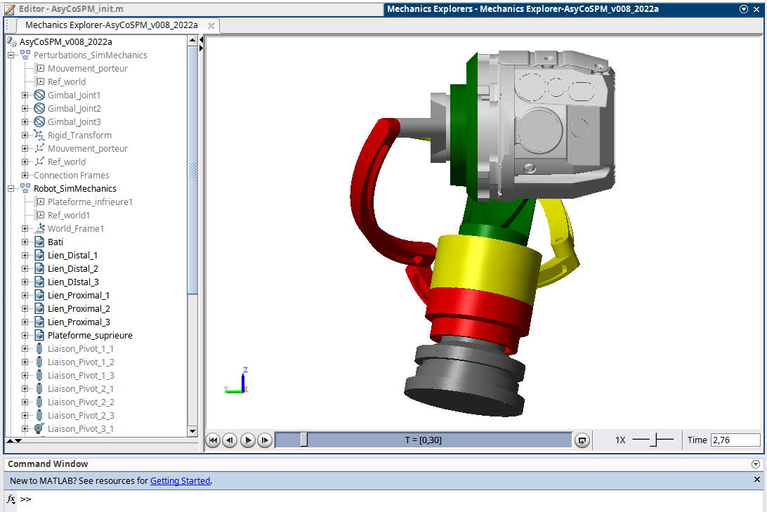
Figure 14: Digital model of the SPM

In this last simulation, we implemented a digital model of the spherical parallel robot and its speed control in a Matlab Simulink^® environment (here 2022a). The latter is interfaced with the Catia files of the mechanism via SimMechanics™. Figure 14 shows the screenshot of the before-mentioned digital model.

Such a model allows us to have an overview of the dynamics of the robot. It is in this regard complementary to the kinematic study of the mechanism discussed in this article. For instance, one can evaluate the torque $\bm{\tau}\triangleq\left[\;\begin{matrix}\tau_{1}&\tau_{2}&\tau_{3}\end{matrix}\;\right]^{\mathsf{T}}$ required to move the several actuators, as shown in Figure 15, where $\tau_{i}$ denotes the torque applied to the $i$^th actuator.

[width=]TikZ/AsyCoSPM_1_TAU_trans

(a) Transient state

[width=]TikZ/AsyCoSPM_1_TAU_perm

(b) Steady state

Figure 15: Motor torque of the SPM

These curves show that the engine torques required to stabilize the LOS are reasonable: one obtains torques in absolute values that do not exceed $4\,\text{Nm}$ in the transient state and $2.5\,\text{Nm}$ in steady state.

4 Conclusion & outlook

This paper discussed on the use of a 3-DOF Spherical Parallel Manipulator with coaxial shafts that embeds a sight device for the inertial LOS stabilization. Having at disposal its kinematic model, it has been shown that a speed control loop achieves the disturbance rejection taking into account the motion of the carrier as well as the friction torque undergone by the actuators. Such results are also verified with the SimMechanics™ digital model of our robot simulating its dynamics.

Although the kinematics of the robot is certified for our regular workspace, the control strategy is not. Indeed, the inertial speed reference can in fact make the mechanism leave the safe region without knowing it. In this case, one cannot guaranty the good behavior of the device and its control. By the same logic, the current control loop does not take into account uncertainties on the system that can bring instability in the worst case. In this regard, further works will focus on the robustness of the system and a management of the joint stops to avoid the robot leaving the safe regions. Such aspects will bring the certification to the speed control.

As the article mainly focused on the kinematics of the robot, an interesting outlook could be diving into the dynamic model of the latter.

[width=2]TikZ/spm_chaine_cinematique

Figure 16: Kinematic chain of a general SPM

Appendix A Derivation of the geometric model of the 3-RRR 3-DOF SPM of interest

A.1 Expressions of the unit vectors

Based on the convention used in [Lê et al., 2023] and [Bai et al., 2009], one can obtain the unit vectors $\bm{u}_{i}$, $\bm{w}_{i}$, and $\bm{v}_{i}$, with $i\in\left\llbracket 1,3\right\rrbracket$ by exploiting the kinematic chain of the robot depicted in Figure 16.

Given that $\bm{z}_{\mathfrak{b}}\triangleq\left[\;\begin{matrix}0&0&1\end{matrix}\;\right]^{\mathsf{T}}$, one can show that they can be written in the reference frame $\mathcal{F}_{\mathfrak{b}}\coloneqq\left(O,\bm{x}_{\mathfrak{b}},\bm{y}_{\mathfrak{b}},\bm{z}_{\mathfrak{b}}\right)$ as:

$$\prescript{\mathfrak{b}}{}{\bm{u}_{i}} =\bm{R}_{z}{\left(\eta_{i}\right)}\,\bm{R}_{x}{\left(\beta_{1}-\pi\right)}\,\bm{z}_{\mathfrak{b}}$$ (21)

$$\prescript{\mathfrak{b}}{}{\bm{w}_{i}} =\bm{R}_{z}{\left(\eta_{i}\right)}\,\bm{R}_{x}{\left(\beta_{1}-\pi\right)}\,\bm{R}_{z}{\left(\theta_{i}\right)}\,\bm{R}_{x}{\left(\alpha_{1,i}\right)}\,\bm{z}_{\mathfrak{b}}$$

$$\prescript{\mathfrak{b}}{}{\bm{v}_{i}} =\bm{R}_{z}{\left(\chi_{3}\right)}\bm{R}_{y}{\left(\chi_{2}\right)}\bm{R}_{x}{\left(\chi_{1}\right)}\bm{R}_{z}{\left(\eta_{i}\right)}\,\bm{R}_{x}{\left(-\beta_{2}\right)}\,\bm{z}_{\mathfrak{b}}$$

where $\bm{R}_{x}$, $\bm{R}_{y}$ and $\bm{R}_{z}$ denote the rotation matrices around their respective local axis. The latter matrices are defined as follows:

$$\bm{R}_{x}(\chi_{1}) \triangleq\left[\;\begin{matrix}1&0&0\\ 0&\cos\left(\chi_{1}\right)&-\sin\left(\chi_{1}\right)\\ 0&\sin\left(\chi_{1}\right)&\cos\left(\chi_{1}\right)\end{matrix}\;\right]$$ (22a)

$$\bm{R}_{y}(\chi_{2}) \triangleq\left[\;\begin{matrix}\cos\left(\chi_{2}\right)&0&\sin\left(\chi_{2}\right)\\ 0&1&0\\ -\sin\left(\chi_{2}\right)&0&\cos\left(\chi_{2}\right)\end{matrix}\;\right]$$ (22b)

$$\bm{R}_{z}(\chi_{3}) \triangleq\left[\;\begin{matrix}\cos\left(\chi_{3}\right)&-\sin\left(\chi_{3}\right)&0\\ \sin\left(\chi_{3}\right)&\cos\left(\chi_{3}\right)&0\\ 0&0&1\end{matrix}\;\right]$$ (22c)

Remark 3.

The disposition of the pivot linkage $\eta_{i}$, $i\in\left\llbracket 1,3\right\rrbracket$ is supposed to be identical for the base and the upper platform, as in [Lê et al., 2023]. However, as our robot has coaxial input shafts ($\beta_{1}=0$), such parameters does not appear “physically” but still in the equations.

Remark 4.

In the special case of SPMs with coaxial input shafts ($\beta_{1}=0$), one always has

$$\prescript{\mathfrak{b}}{}{\bm{u}_{i}}=\left[\;\begin{matrix}0\\ 0\\ -1\end{matrix}\;\right],\qquad\forall\,i\in\left\llbracket 1,3\right\rrbracket$$

as mentioned in [Tursynbek and Shintemirov, 2020].

A.2 Expression of the geometric model

Let $x_{i}=\cos{\left(\chi_{i}\right)}$, $y_{i}=\sin{\left(\chi_{i}\right)}$, $c_{i}=\cos{\left(\theta_{i}\right)}$, and $s_{i}=\sin{\left(\theta_{i}\right)}$, $i\in\left\llbracket 1,3\right\rrbracket$. The detailed geometric model of the mechanism of interest is given by:

$$\hskip 12.50002pt\bm{f}(\bm{\theta},\bm{\chi})=\left[\;\begin{matrix}f_{1}(\theta_{1},\chi_{1},\chi_{2},\chi_{3})\\ f_{2}(\theta_{2},\chi_{1},\chi_{2},\chi_{3})\\ f_{3}(\theta_{3},\chi_{1},\chi_{2},\chi_{3})\end{matrix}\;\right],\quad\text{with}$$ (23)

$$f_{1} =-c_{1}x_{3}y_{2}y_{1}+s_{1}x_{3}y_{2}y_{1}+c_{1}y_{3}y_{2}y_{1}+s_{1}y_{3}y_{2}y_{1}$$

$$\hskip 30.00005pt-x_{2}y_{1}\sqrt{2}+c_{1}x_{3}x_{1}+s_{1}x_{3}x_{1}+c_{1}y_{3}x_{1}$$

$$\hskip 30.00005pt-s_{1}y_{3}x_{1}+c_{1}x_{3}x_{2}-s_{1}x_{3}x_{2}$$

$$\hskip 30.00005pt-c_{1}y_{3}x_{2}-s_{1}y_{3}x_{2}-y_{2}\sqrt{2}$$

$$f_{2} =c_{2}x_{3}y_{2}y_{1}+s_{2}x_{3}y_{2}y_{1}+c_{2}y_{3}y_{2}y_{1}-s_{2}y_{3}y_{2}y_{1}$$

$$\hskip 30.00005pt-x_{2}y_{1}\sqrt{2}+c_{2}x_{3}x_{1}-s_{2}x_{3}x_{1}-c_{2}y_{3}x_{1}$$

$$\hskip 30.00005pt-s_{2}y_{3}x_{1}+c_{2}x_{3}x_{2}+s_{2}x_{3}x_{2}$$

$$\hskip 30.00005pt+c_{2}y_{3}x_{2}-s_{2}y_{3}x_{2}+y_{2}\sqrt{2}$$

$$f_{3} =c_{3}y_{1}y_{2}y_{3}+s_{3}x_{3}y_{1}y_{2}+c_{3}x_{1}x_{3}-s_{3}x_{1}y_{3}$$

As highlighted in Figure 16, such a system is obtained using a kinematic closure being the dot product between $\bm{w}_{i}$ and $\bm{v}_{i}$, $i\in\left\llbracket 1,3\right\rrbracket$.

References

- [Bai et al., 2009] Bai, S., Hansen, M. R., and Angeles, J. (2009). A robust forward-displacement analysis of spherical parallel robots. Mechanism and Machine Theory, 44:2204–2216.
- [Gosselin and Hamel, 1994] Gosselin, C. and Hamel, J.-F. (1994). The agile eye: a high-performance three-degree-of-freedom camera-orienting device. In Proceedings of the 1994 IEEE International Conference on Robotics and Automation, pages 781–786 vol.1.
- [Hilkert, 2008] Hilkert, J. (2008). Inertially stabilized platform technology concepts and principles. IEEE Control Systems Magazine, 28(1):26–46.
- [Kantorovich, 1948] Kantorovich, L. V. (1948). On Newton’s method for functional equations. Functional Analysis and Applied Mathematics, 59(7):1237–1240.
- [Lazard and Rouillier, 2007] Lazard, D. and Rouillier, F. (2007). Solving parametric polynomial systems. Journal of Symbolic Computation, 42(6):636–667.
- [Lê et al., 2023] Lê, A., Rouillier, F., Rance, G., and Chablat, D. (2023). On the Certification of the Kinematics of 3-DOF Spherical Parallel Manipulators. Maple Transactions.
- [Masten, 2008] Masten, M. K. (2008). Inertially stabilized platforms for optical imaging systems. IEEE Control Systems Magazine, 28(1):47–64.
- [Merlet, 2006] Merlet, J.-P. (2006). Parallel Robots (Second Edition). Solid Mechanics and Its Application. Springer.
- [Rouillier, 2007] Rouillier, F. (2007). Algorithmes pour l’étude des solutions réelles des systèmes polynomiaux. Habilitation à diriger des recherches, Université Pierre & Marie Curie - Paris 6.
- [Tursynbek and Shintemirov, 2020] Tursynbek, I. and Shintemirov, A. (2020). Infinite torsional motion generation of a spherical parallel manipulator with coaxial input axes. 2020 IEEE/ASME International Conference on Advanced Intelligent Mechatronics (AIM), pages 1780–1785.