Efficient Microwave Spin Control of Negatively Charged Group-IV Color Centers in Diamond

Abstract

In this work, we provide a comprehensive overview of the microwave-induced manipulation of electronic spin states in negatively charged group-IV color centers in diamond with a particular emphasis on the influence of strain. Central to our investigation is the consideration of the full vectorial attributes of the magnetic fields involved, which are a dc field for lifting the degeneracy of the spin levels and an ac field for microwave control between two spin levels. We observe an intricate interdependence between their spatial orientations, the externally applied strain, and the resultant efficacy in spin state control. In most work to date the ac and dc magnetic field orientations have been insufficiently addressed, which has led to the conclusion that strain is indispensable for the effective microwave control of heavier group-IV vacancies, such as tin- and lead-vacancy color centers. In contrast, we find that the alignment of the dc magnetic field orthogonal to the symmetry axis and the ac field parallel to it can make the application of strain obsolete for effective spin manipulation. Furthermore, we explore the implications of this field configuration on the spin’s optical initialization, readout, and gate fidelities.

I Introduction

For many quantum information applications [1] such as quantum sensing [2], quantum networks [3, 4] and quantum computing [5], key requirements include ultra-high fidelity initialization, both single and two-qubit gate operations, as well as readout. Notably, the execution of quantum algorithms that offer a quantum advantage [6] demand near-perfect operations within the coherence time of the system. In particular, the fidelity of single-qubit gates now consistently exceeds 99% across diverse platforms, including superconducting qubits [7], quantum dots [8], trapped ions [9], and ultra-cold atoms [10].

An emerging class of optically active spin-1/2 systems for quantum information applications is found in negatively charged group-IV color centers in diamond (G4Vs) [11], including silicon (SiV), germanium (GeV), tin (SnV), and lead vacancy center (PbV). G4Vs exhibit notably high optical efficiency, with a Debye-Waller factor of 60-80% [12, 13, 14]), in contrast to the 3% Debye-Waller factor observed in the negatively charged nitrogen vacancy center [15]. Moreover, they display lower sensitivity to electric noise [16], rendering them highly suitable for integration into nanostructures [3, 17], which is crucial for efficient coupling to a precisely defined optical mode [18]. Furthermore, G4Vs exhibit excellent spin coherence times, with, for example, the GeV showing $T_{2}=20$ ms [19].

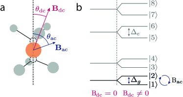
Figure 1: Illustration of the physical system. a) group-IV color center with the respective angles of the dc magnetic field ${\bf B}_{\rm dc}$ and the ac driving field ${\bf B}_{\rm ac}$ relative to the symmetry axis. b) Level scheme of the defect without and with an external dc magnetic field, which lifts the spin degeneracy. The qubit driven by ${\bf B}_{\rm ac}$ is composed of the states $|1\rangle$ and $|2\rangle$.

This work primarily focuses on the theoretic analysis of single-qubit gates acting on the electronic spin, which operate in the microwave regime. In the first works demonstrating coherent microwave control of the SnV [20, 21] a consensus has emerged, which asserts that strain is an essential prerequisite for manipulating the spin of the heavier implanted group-IV elements such as tin and lead, owing to their increased spin-orbit coupling in comparison to lighter elements like silicon and germanium. Consequently, we are particularly interested in the interplay of strain and spin-orbit coupling in the investigation of coherent control of the spin qubit.

Interestingly, we discovered a magnetic field configuration, for which strain is not only unnecessary but actually hampers the efficiency of the coherent control. As we will demonstrate that the efficiency depends on the orientation of the static field ${\bf B}_{\rm dc}$, which is necessary to lift the spin degeneracy, and the oscillating field ${\bf B}_{\rm ac}(t)$, responsible for driving the electronic spin (see Fig. 1a).

This work is structured as follows: We first provide a brief overview of the static contributions to the systems Hamiltonian, such as the spin-orbit coupling, the Jan-Teller effect, the interaction with internal and external strain as well as the static magnetic field ${\bf B}_{\rm dc}$. We then introduce the influence of ${\bf B}_{\rm ac}(t)$ and explain how such a field generates single-qubit gates acting on the two energetically lowest lying qubit states $|1\rangle$ and $|2\rangle$ (see Fig.1b).

We find a closed approximate expression for the qubit’s Rabi frequency $\Omega$ as a function of total strain acting on the G4V, the spin orbit coupling and the magnetic fields ${\bf B}_{\rm dc}$ and ${\bf B}_{\rm ac}$. The Rabi frequency $\Omega$ is a key performance metric for the driving efficiency: The bigger $\Omega$ for a given magnetic field strength $B_{\rm ac}$, the more efficient magnetic control becomes. Enhanced control efficiency leads to a reduced need for microwave power, resulting in lower levels of heating and, in broader terms, a decrease in the experimental overhead needed for spin control. Notably, the most efficient control doesn’t require strain but strain becomes detrimental independent of the G4V.

Finally we analyse initialization and readout based on the master equations in Lindblad form for various configurations of the magnetic field, and find that for the most efficient control regime, both are possible.

II Microwave gates

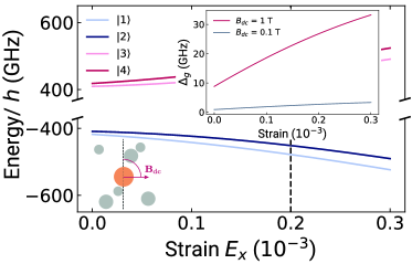
Figure 2: The relative energies of the ground state orbital branches $|1\rangle,|2\rangle$ and $|3\rangle,|4\rangle$ of the SnV as a function of strain in the presence of $B_{\rm dc}=1$ T oriented perpendicular to the symmetry axis. The value of 1 T is used to enhance the visibility of the splitting. The inset shows the splitting $\Delta_{g}$ between $|1\rangle$ and $|2\rangle$ for $B_{\rm dc}=0.1$ T and 1 T. The dashed vertical line marks a comparatively large but experimentally realistic strain value [22]. For $B_{\rm dc}>0.1$ T the ground state splitting $\Delta_{g}>1/\tau_{\rm rad}$, where $\tau_{\rm rad}=4.5$ ns is the radiative lifetime of the SnV [23].

We decompose the total magnetic field at the position of the SnV into a static dc and time-dependent ac part ${\bf B}(t)={\bf B}_{\rm dc}+{\bf B}_{\rm ac}(t)$, where ${\bf B}_{\rm ac}$ is either the near-field of an alternating current passing through a stripline in close proximity to the defect, or the far field of a microwave source. In this work, irrespective of the generation ${\bf B}_{\rm ac}(t)$ is referred to as the microwave drive of the system.

Based on the decomposition of the magnetic field we split the Hamiltonian generating the time evolution of the system into a dc and ac component

$$H(t)=H_{\rm dc}+H_{\rm ac}(t)\leavevmode\nobreak\ ,$$ (1)

where $H_{\rm dc}$ generates the free evolution and $H_{\rm ac}$ is the interaction of the system with $B_{\rm ac}(t)$. We assume that $B_{\rm ac}(t)$ drives the system for some finite gate time $T_{\rm G}$. The single-qubit gate operating on the electronic spin is then given by

$$U(t_{e},t_{i})=Te^{\frac{{\rm i}}{\hbar}\int_{t_{i}}^{t_{e}}H(t)\mathrm{d}t}\leavevmode\nobreak\ ,$$ (2)

where $T_{\rm G}=t_{e}-t_{i}$ and $T$ is the time-ordering operator. We will confirm that indeed any desired single qubit gate $U\in$ SU(2) can be constructed with a suitable series of control pulses associated to $H(t)$. In the following we detail the interactions contributing to $H_{\rm dc}$ and $H_{\rm ac}$. We separate $H_{\rm dc}$ into

$$H_{\rm dc}=H_{\rm int.}+H_{\rm ext.}$$ (3)

Where $H_{\rm int.}$ contains all the terms that are intrinsic to the diamond system and $H_{\rm ext.}$ contains terms such as externally applied strain or the static field ${\bf B}_{\rm dc}$.

The intrinsic components are

$$H_{\rm int.}=H_{0}+H_{\rm SO}+H_{\rm JT}+H_{\rm int.\leavevmode\nobreak\ strain}\leavevmode\nobreak\ ,$$ (4)

where $H_{0}$ describes the unperturbed effective single particle system. The general structure of all contributions to $H_{\rm dc/ac}$ can be deduced from group theory and the D_3d symmetry of the unperturbed system associated to G4V defects [24]. $H_{\rm SO}$ is the spin orbit interaction and $H_{\rm JT}$ describes the Jahn-Teller effect. Finally, $H_{\rm int.\leavevmode\nobreak\ strain}$ is the internal strain, which is not intrinsic to the vacancy but intrinsic to the diamond and cannot be easily manipulated. Internal strain can have many causes, such as the displacement of lattice atoms by interstitial crystal impurities [25], lattice vacancies such as mono-, di- or multi-vacancy complexes [26] and lattice dislocations [27].

In contrast to $H_{\rm int.\leavevmode\nobreak\ strain}$, the contribution $H_{\rm intrinsic}=H_{0}+H_{\rm SO}+H_{\rm JT}$ is the same for all defects of the same class, if no other perturbations are present. In this work we explicitly separate $H_{\rm int.\leavevmode\nobreak\ strain}$ and $H_{\rm JT}$. Sometimes both terms are combined in $H_{\rm int.\leavevmode\nobreak\ strain}$ or simply in $H_{\rm strain}$, due to their structural similarity.

The extrinsic components to $H_{\rm dc}$ are

$$H_{\rm ext.}=H_{\rm ext.\leavevmode\nobreak\ strain}+H_{\rm B_{\rm dc}}$$ (5)

The dc component of the magnetic field lifts the spin degeneracy through the Zeeman term and therefore makes the spin degree of freedom accessible to microwave control.

In the following we describe the explicit structure of the interaction terms. Following [24] a basis for an explicit representation of the interactions can be chosen using group theoretic arguments based on the D_3d symmetry. For the discussion of the microwave control we focus on the ground state manifold, which is spanned by the four states

$$|e_{gx}\uparrow\rangle,\leavevmode\nobreak\ |e_{gx}\downarrow\rangle,\leavevmode\nobreak\ |e_{gy}\uparrow\rangle,\leavevmode\nobreak\ |e_{gy}\downarrow\rangle\leavevmode\nobreak\ ,$$ (6)

which are energetically degenerate eigenstates of $H_{0}$ belonging to the $E$ irreducible representation. The two orbital states labeled with $e_{gx/gy}$ have even symmetry and are two fold spin degenerate. Due to the degeneracy we can drop the $H_{0}$ contribution to the Hamiltonian and focus on the representation of the other internal and external contributions to the Hamiltonian. From [24] the representations of the various contributions are in the above basis (6):

$$H_{\rm SO}=\begin{pmatrix}0&-i\lambda\\ i\lambda&0\\ \end{pmatrix}\otimes\begin{pmatrix}1&0\\ 0&-1\\ \end{pmatrix}$$ (7)

where $\lambda$ is the spin-orbital coupling. Note that compared to [24] we absorbed the $1/2$ into $\lambda$.

$$H_{\rm JT}=\begin{pmatrix}\Upsilon_{x}&\Upsilon_{y}\\ \Upsilon_{y}&-\Upsilon_{x}\\ \end{pmatrix}\otimes\begin{pmatrix}1&0\\ 0&1\\ \end{pmatrix}$$ (8)

where $\Upsilon_{x}$ and $\Upsilon_{y}$ are the Jahn-Teller coupling strengths.

The external and internal strain contributions are:

$$H_{\rm S}=\begin{pmatrix}dE_{x}&2d\epsilon_{xy}\\ 2d\epsilon_{xy}&-dE_{x}\\ \end{pmatrix}\otimes\begin{pmatrix}1&0\\ 0&1\\ \end{pmatrix}$$ (9)

where

$$E_{x}=\epsilon_{xx}-\epsilon_{yy}\leavevmode\nobreak\ ,$$ (10)

$\epsilon_{xx}$, $\epsilon_{yy}$ and $\epsilon_{xy}$ are the strain tensor elements representing uni-axial stress and $d$ is the spin-strain coupling strength. For $H_{\rm int.\leavevmode\nobreak\ strain}$ and $H_{\rm ext.\leavevmode\nobreak\ strain}$ we discriminate between $E_{x}^{\rm int.},\epsilon_{\rm xy}^{\rm int.}$ and $E_{x}^{\rm ext.},\epsilon_{\rm xy}^{\rm ext.}$. For the sake of brevity, we drop the superscript from the external contribution. The degeneracy of the four basis states is lifted due to $H_{\rm SO}$, $H_{\rm JT}$ and $H_{\rm int.strain}$.

The static magnetic field $B_{\rm dc}$ lifts the spin degeneracy, which is required to turn the long lived spin states into a qubit that is amenable to microwave control. Magnetic fields couple to the vacancy according to [24]

$$H_{\rm B} =H_{\parallel}+H_{\perp}$$

$$\begin{aligned} =f&\gamma_{L}B_{z}\begin{pmatrix}0&i\\ -i&0\end{pmatrix}\otimes\begin{pmatrix}1&0\\ 0&1\\ \end{pmatrix}\\ +&\gamma_{S}\begin{pmatrix}1&0\\ 0&1\\ \end{pmatrix}\otimes\begin{pmatrix}B_{z}&B_{x}-{\rm i}B_{y}\\ B_{x}+{\rm i}B_{y}&-B_{z}\\ \end{pmatrix}\end{aligned}$$ (11)

where the magnetic field is ${\bf B}=(B_{x},B_{y},B_{z})$, and the $z$-direction is aligned with defect’s symmetry axis. Furthermore, $f=0.15$ is a coupling constant and

$$\gamma_{L}=\frac{\gamma_{S}}{2}=\frac{\mu_{B}}{\hbar}\leavevmode\nobreak\ ,$$ (12)

where $\mu_{B}$ is the Bohr magneton. Both the ${\bf B}_{\rm dc}$ and ${\bf B}_{\rm ac}(t)$ fields couple to the system through Eq. (11).

	$2\lambda$ (GHz)	$\Upsilon_{x}$ (GHz)	$\Upsilon_{y}$ (GHz)	f	$d$ (PHz/Strain)
Ground States
SiV	49	2	3	0.1	1.3
GeV	207	NA	NA	NA	NA
SnV	815	65	0	0.15	0.787
PbV	4385	NA	NA	NA	NA
Excited States
SiV	257	12	16	0.1	1.8
GeV	989	NA	NA	NA	NA
SnV	2355	855	0	0.15	0.956
PbV	6920	NA	NA	NA	NA

Table 1: Parameter used in this paper for SiV [28, 22], GeV [11], SnV [23, 21] and PbV [11]. $\lambda$ is the spin-orbital coupling, $\Upsilon_{x}$ and $\Upsilon_{y}$ are the Jahn-Teller coupling strengths, $f$ is the quenching factor of $\gamma_{L}$, and $d$ is the spin-strain coupling constant. The SiV and GeV are categorized as light color centers, while the SnV and PbV are designated as heavy color centers.

In Fig. 1a, we illustrate the field orientations with respect to the defect’s symmetry axis. In Fig. 1b we show the G4V energy levels including the excited states. The eigenstates of $H_{\rm dc}$ are then comprised of the four ground states ($|1\rangle$-$|4\rangle$). For the sake of completeness, we also included the four excited states ($|4\rangle$-$|8\rangle$). For the remainder of this work we refer to zero strain as the $H_{\rm ext.strain}=\mathbf{0}$.

As an example, we show in Fig. 2 the energy levels of the SnV’s ground states as a function of strain at $B_{\rm dc}=1$T (we use $1$ T to enhance the visibility of behaviors), orthogonal to the symmetry axis. Strain increases both the splitting between the orbital branches $|1\rangle,|2\rangle$ and $|3\rangle,|4\rangle$, which can lead to increased spin coherence times as thermal decoherence channels are reduced [29]. The inset shows the splitting $\Delta$ between $|1\rangle$ and $|2\rangle$, which is $\propto B_{\rm dc}$. In Table 1 we present established model parameters for the light G4V (SiV and GeV) and the heavy G4V (SnV and PbV).

Having set up a full model of the physical systems under consideration, we can now analyze the interplay of strain and the implementation of microwave enabled gates acting on the spin degree of freedom. For that purpose we begin with diagonalizing $H_{\rm dc}$ and writing $H_{\rm B_{\rm ac}(t)}$ in terms of the eigenstates of $H_{\rm dc}$ (see appendix A). The diagonalization of $H_{\rm dc}$ is done in two steps: First we diagonalize $H=H_{\rm int}+H_{\rm ext.strain}$, for which we find two two-fold spin degenerate eigenstates with energies

$$e_{\pm,\downarrow\uparrow}=\pm\sqrt{\lambda^{2}+\xi^{2}}\leavevmode\nobreak\ ,$$ (13)

where $\xi^{2}=\upsilon_{x}^{2}+\upsilon_{y}^{2}$, $\upsilon_{x}=(dE_{x}+\Upsilon_{x})$, $\upsilon_{y}=(2d\epsilon_{xy}+\Upsilon_{y})$, $E_{x}=E_{x}^{\rm int}+E_{x}^{\rm ext}$ and $\epsilon_{xy}=\epsilon_{xy}^{\rm int.}+\epsilon_{xy}^{\rm ext.}$. We then re-express $H_{\rm B_{\rm dc}}$ in the energy eigenbasis $|e_{-},\downarrow\rangle,|e_{-},\uparrow\rangle,$ $|e_{+},\downarrow\rangle,|e_{+},\uparrow\rangle$. The detailed expressions can be found in the appendix A. We can remove the states $|e_{+},\uparrow\downarrow\rangle$ through adiabatic elimination as long as $2e_{+,\downarrow}$ is bigger than any other energy in the problem [30]. This reduction places certain limits on the magnetic field strengths and strain regimes for which the approximation is valid.

The reduction of the system results in

$$H_{\rm eff}=-\frac{\Delta_{g}}{2}\sigma_{z}-{\bf S}\cdot\hat{\bm{\mu}}\cdot{\bf B}_{\rm ac}(t)\leavevmode\nobreak\ ,$$ (14)

where

$$\Delta_{g}=2\gamma_{s}\sqrt{\sin(x)^{2}(B_{x,{\rm dc}}^{2}+B_{y,{\rm dc}}^{2})+\Theta(B_{z,\rm dc})^{2}}\leavevmode\nobreak\ ,$$ (15)

$$\Theta(B_{z,dc})=-B_{z,dc}\left(f\frac{\gamma_{l}}{\gamma_{s}}\cos(x)+1\right)\leavevmode\nobreak\ ,$$ (16)

and the 3$\times$3 matrix $\bm{\mu}$ depends on ${\bf B}_{\rm dc}=[B_{x{\rm,dc}},B_{y{\rm,dc}},B_{z{\rm,dc}}]$ as well as $\xi$ (see appendix A for details). We also use ${\bf S}=\bm{\sigma}/2$, $\bm{\sigma}=(\sigma_{x},\sigma_{y},\sigma_{z})$ ($\sigma_{i}$ are the Pauli matrices) and $\tan(x)=\xi/\lambda$.

In the case of ${\bf B}_{\rm ac}(t)=b(t){\bf B}_{\rm ac}\cos(\omega t)$, where $b(t)$ changes on timescales that are slow compared to the other time-scales in the problem, $H_{\rm eff}$ in Eq. (14) can be treated in the rotating-wave approximation as (see appendix B)

$$H_{\rm eff}^{\rm RWA}=b(t)\Omega{\bf n}\cdot\bm{\sigma}$$ (17)

where ${\bf n}=[(\hat{\bm{\mu}}\cdot{\bf B}_{\rm ac})_{x}/2,(\hat{\bm{\mu}}\cdot{\bf B}_{\rm ac})_{y}/2,0]/\Omega$. If we further introduce

$${\bf B}_{\rm dc/ac} =B_{\rm dc/ac}\begin{bmatrix}\cos(\phi_{\rm dc/ac})\sin(\theta_{\rm dc/ac})\\ \sin(\phi_{\rm dc/ac})\sin(\theta_{\rm dc/ac})\\ \cos(\theta_{\rm dc/ac})\end{bmatrix}\leavevmode\nobreak\$$ (18)

we find

$$\Omega=\gamma_{s}B_{\rm ac}\Lambda\leavevmode\nobreak\ ,$$ (19)

$$\begin{aligned} &\Lambda=\sin(x)\sqrt{\begin{aligned} &\Xi(\phi,\theta_{\rm ac})^{2}\\ &\hskip 14.22636pt+\frac{\chi(\phi,\theta_{\rm dc},\theta_{\rm ac})^{2}}{\sin(\theta_{\rm dc})^{2}\zeta(x)^{2}+\cos(\theta_{\rm dc})^{2}}\end{aligned}}\end{aligned}\leavevmode\nobreak\ ,$$ (20)

where

$$\Xi(\phi,\theta_{\rm ac})=\sin(\phi)\sin(\theta_{\rm ac})$$ (21)

$$\begin{aligned} \chi(\phi,\theta_{\rm dc},\theta_{\rm ac})=&\sin(\theta_{\rm dc})\cos(\theta_{\rm ac})\\ &\hskip 14.22636pt-\cos(\phi)\cos(\theta_{\rm dc})\sin(\theta_{\rm ac})\end{aligned}$$ (22)

$\zeta(x)=\sin(x)/[f\cos(x)/2+1]$ and $\phi=\phi_{\rm dc}-\phi_{\rm ac}$. The coupling strength $\Lambda$ provides analytical insight into the most efficient microwave control regime.

$H_{\rm eff}^{\rm RWA}$ can handily be interpreted as a Hamiltonian that generates rotations around the ${\bf n}$ axis on the Bloch sphere. The gate defined in Eq. (2), then becomes in the rotating frame

$$U(t_{e},t_{i})=e^{\frac{i}{\hbar}\theta{\bf n}\cdot\bm{\sigma}}\leavevmode\nobreak\ ,$$ (23)

where $\theta=\Omega\int_{t_{i}}^{t_{e}}f(t)\mathrm{d}t$. Any element in $SU(2)$ (i.e. any rotation on the Bloch sphere), can be constructed by composing $U=R_{x}(\alpha)R_{y}(\beta)R_{x}(\gamma)$, where $R_{x/y}(\alpha)$ are rotations around the $x$ or $y$ axis on the Bloch sphere by an angle $\alpha$ [31]. Both rotational axis are accessible by either adjusting the phase of the ac driving field ${\bf B}_{\rm ac}(t)\rightarrow f(t){\bf B}_{\rm ac}\cos(\omega t+\varphi)$ or by changing the orientation of ${\bf B}_{\rm ac}$ to switch between $x$ and $y$ axis (see e.g. Eq. (17)). We comment on numerically obtained gate fidelities of $U(t_{e},t_{i})$ without any approximations after discussing the control efficacy of the SiV and SnV.

III Efficient Microwave control

The most efficient regime for microwave control can be determined by $\Lambda$ given in Eq. (20). Having a closed expression for $\Lambda$ allows us to make some general statements about the efficiency of control for different strain regimes and orientations of ${\bf B}_{\rm ac/dc}$. We first analyze general properties of $\Lambda$ as a function of $x$ and then discuss $\Lambda$’s dependence on the orientations of ${\bf B}_{\rm dc}$ and ${\bf B}_{\rm ac}$.

Notably, Eq. (20) only depends on the difference of the azimuthal angles $\phi_{\rm dc}-\phi_{\rm ac}$, the polar angles $\theta_{\rm dc}$, $\theta_{\rm ac}$ and the dimensionless variable $x\in\{0,\pi/2\}$. The fact that $\xi$ solely enters through its comparison with the spin orbit interaction $\lambda$ is another interesting feature of Eq. (20), which allows for a general discussion of the interplay of strain, the Jan-Teller effect and the spin orbit interaction, completely independent of the G4V.

With very little effort we can assert that $\Lambda=0$ for ${\bf B}_{\rm ac}$ parallel ${\bf B}_{\rm dc}$, which is in line with physical intuition: no driving of the spin-qubit is possible in the absence of spin-mixing. Before investigating the local extrema of $\Lambda$, we analyze the limits $\xi\rightarrow 0$ and $\xi\rightarrow\infty$, which correspond to $x=0$ and $x=\pi/2$, respectively.

For small values $x\rightarrow 0$, we expand $\Lambda$ in leading orders of $x$:

$$\lim_{x\rightarrow 0}\Lambda=f(\phi,\theta_{\rm ac},\theta_{\rm dc})x+\mathcal{O}(x)^{2}$$ (24)

where $f(\phi,\theta_{\rm ac},\theta_{\rm dc})$ can be found in appendix C.

It would appear that $\Lambda=0$ for $x=0$, corresponding to an absence of the Jahn-Teller interaction, as well as internal and external strain. Interestingly, as we will explain in the next paragraphs, this is not true for all directions of the magnetic field so that $\Lambda\neq 0$ for $x=0$ under certain conditions.

For $x\rightarrow\infty$, we find that

$$\lim_{\xi\rightarrow\infty}\Lambda=g(\phi,\theta_{\rm dc},\theta_{\rm ac})$$ (25)

where $g(\phi,\theta_{\rm dc},\theta_{\rm ac})$ only depends on the magnetic fields’ orientations (see appendix C), sometimes referred to as the free electron limit [20]. Notably, this is the case for either $\xi\rightarrow\infty$ or $\lambda\rightarrow 0$, which means that as long as the strain outcompetes the spin-orbit coupling, the efficiency of the driving will purely depend on the relative orientation of ${\bf B}_{\rm dc}$ and ${\bf B}_{\rm ac}$.

Local extrema of $\Lambda$ as a function of $\phi$, $\theta_{\rm dc}$ and $\theta_{\rm ac}$ can be found analytically. The first extremum of interest is $\phi=0$ deg$,\leavevmode\nobreak\ \theta_{\rm dc}=0$ deg and $\theta_{\rm ac}=90$ deg, which corresponds to ${\bf B}_{\rm dc}$ being parallel to the main symmetry axis of the G4V, and ${\bf B}_{\rm ac}$ being oriented in the $xy$-plane. For this combination of angles $\Lambda_{1}=\sin(x)$.

For infinite strain, i.e. $x=\pi/2$, the coupling is maximized $\Lambda_{1}=1$ and $\Lambda_{1}=0$ for zero strain and zero Jahn Teller interaction, which is in accordance with previous reports on microwave control [20, 21]. In the case of $\xi<\lambda$ we can reproduce the finding in [32], where $\Omega=\gamma_{s}B_{\rm ac}\sqrt{\upsilon_{x}^{2}+\upsilon_{y}^{2}}/\lambda$. One can show that this extremum is a saddle point as a function the two polar angles of the magnetic fields (see Fig. 3), which means there exist orientations, that allow for more efficient control. The difference of the azimuths $\phi$ has little impact on the steepness of the saddle point, which means that changing the azimuthal orientation of the fields will have little impact on the driving efficiency.

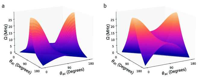
Figure 3: Rabi frequency $\Omega$ as a function of the magnetic field angles $\theta_{\rm dc}$ and $\theta_{\rm ac}$ unstrained (a) and strained ($E_{x}=0.2\,\times 10^{-3}$) (b) for the SnV, $B_{\rm dc}=100$ mT.

The second notable local extremum is given by $\phi=0$ deg$,\theta_{\rm dc}=90$ deg$,\theta_{\rm ac}=0$ deg, which corresponds to ${\bf B}_{\rm dc}$ lying in the $xy$-plane and ${\bf B}_{\rm ac}$ being oriented in parallel to the symmetry axis of the system. For this field configuration

$$\begin{aligned} \Lambda_{2}&=\sin(x)|1/\zeta(x)|\\ &=f\cos(x)/2+1\leavevmode\nobreak\ ,\end{aligned}$$ (26)

which is maximized for $x=0$, meaning for either $\xi\ll\lambda$ or no contribution from either the Jan-Teller interaction or internal and external strain. At $x=0$, $\Delta_{g}=0$, which means that the spin-qubit is energetically degenerate, which would make the spin-qubit optically inaccessible. This, however, is not physical, since there will always be a Jahn-Teller contribution so that $\Delta_{g}\neq 0$. Additionally, for $\Lambda_{2}$, $\Delta_{g}=2\gamma_{s}|\sin(x)|B_{\rm dc}$, the splitting can be increased by increasing $B_{\rm dc}$.

Contrary to $\Lambda_{1}$, $\Lambda_{2}$ is a global extremum as a function of both $\phi$ and the polar angles of the fields. This means that for the most efficient microwave control $\Lambda_{2}$ is the optimum. Their relative magnitude is given by $\Lambda_{2}/\Lambda_{1}=f\cot(x)/2+1/\sin(x)$. Depending on $x$ the magnetic field configuration responsible for $\Lambda_{2}$ can be arbitrarily more effective for controlling the spin-qubit.

We observe that to leading order $\lim_{x\rightarrow 0}(\Lambda-\Lambda_{2})\propto-(\lambda^{4}/\xi^{4})\theta_{\rm dc}^{2}$ for $\theta_{\rm ac}={\rm constant}$, which means that the slope close to $\Lambda_{2}$ becomes infinitely steep for vanishing $\xi$. For emitters with $\lambda<\xi$, the local extrememum is therefore less pronounced. Because $\lambda_{\rm SnV},\lambda_{\rm PbV}\gg\lambda_{\rm SiV}$ more strain should lead to a more forgiving parameter regime for the magnetic fields for efficient spin control of the SnV and PbV. The narrow extremum for larger values of $\lambda$ is also the most likely explanation why $\Lambda_{2}$ so far has evaded experimental detection. The steepness is bound by the Jahn-Teller contribution to $\xi$ and therefore $\xi\neq 0$ for any of the G4V. For the SnV $\Omega$ is shown in Fig. 3. We discuss an optimal control regime in the next section.

IV Optimal control regime

The question of which orientation of the magnetic fields are optimal is highly dependent on the system’s intended use in an application. For most quantum applications, such as the use of the electronic spin as a memory [3], as a nuclear spin interface [33] or as a mediator of entanglement between photons [34] the electronic spin has to be optically addressable, initialized, controlled and read out with high fidelity. Another important aspect is the spin-qubit’s coherence time, which also depends on the dc magnetic field orientation [35]. If the dc magnetic field axis is fixed for a given application, then all of these factors have to be considered. In this section we provide a brief discussion of the important quantities that impact the optimal choice of orientation of the magnetic field.

Optical addressability depends on the difference of $\Delta=|\Delta_{e}-\Delta_{g}|$, where $\Delta_{g}$ and $\Delta_{e}$ are shown in Fig. 1. They can be calculated by replacing $\lambda\rightarrow\Lambda_{e,g}$ in (15). We adopt the convention in [3] that optically addressability requires $\Delta>\Gamma$, where $\Gamma$ in the faster radiative decay rate of the two transitions. This rate depends, of course, on external parameters such as the local density of electromagnetic modes and can be highly influenced by the presence of, for example, a surface boundary or a cavity [36]. The splitting is maximized for the $\theta_{\rm dc}=90$ deg orientation and non-trivially depends on the strain, see Fig. 2. As long as the splitting does not vanish, it can always be increased by increasing the strength of the magnetic field.

The ability to initialize the system is highly dependent on the details of the initialization scheme. Here we briefly discuss two approaches to the spin initialization: Spin pumping [35] and cavity scattering [3].

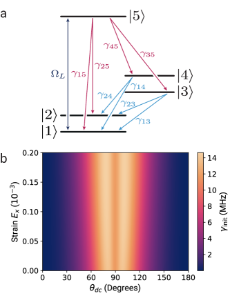
Figure 4: Spin state initialization rate of the SnV defect. a) Level scheme showing the optical (red) and phononic (light blue) relaxation processes $\gamma_{ij}$. The transition $1\leftrightarrow 5$ is resonantly driven by a laser $\Omega_{L}$. b) Initialization rate $\gamma_{\rm intit.}$ as a function of Strain. For most $E_{x}$ values, the highest initialization rates are achieved for ${\bf B}_{\rm dc}$ ($B_{\rm dc}=100$ mT) oriented slightly away from the plane orthogonal to the symmetry axis.

Spin pumping requires the spin initialization rate $\gamma_{\rm init}\gg 1/T_{1}$, where $T_{1}$ is the spin relaxation time of the qubit [35]. For resonant spin pumping we can calculate $\gamma_{\rm init}$ as a function of the relevant spontaneous emission rates and phononic decay processes, as shown in Fig. 4. We use a rate model in the regime of strong pumping $\Omega_{L}\gg\gamma_{15}+\gamma_{25}+\gamma_{35}+\gamma_{45}$, where the rates $\gamma_{ij}$ are illustrated in Fig. 4 and $\Omega_{L}=|\langle 1|{\bf p}\cdot{\bf E}|5\rangle|/2\hbar$ and ${\bf E}$ is the electric field strength of a laser driving the system at the frequency that is resonant with the transition energy $\hbar\omega_{3\downarrow,1\downarrow}$.$\leavevmode\nobreak\ \Omega_{L}$ encodes the cyclicity, which is important for the spin readout. From the rate equations corresponding to Fig. 4a (see appendix F) we find the quasi stationary solution in the strong pumping limit

$$\rho_{11} =e^{-\gamma_{\rm init}t}/2$$ (27)

$$\rho_{22} =1-e^{-\gamma_{\rm init}t}/2$$ (28)

where

$$\gamma_{\rm init}=\frac{\gamma_{25}}{2}\left(1+\frac{\gamma_{35}/\gamma_{25}}{1+\gamma_{13}/\gamma_{23}}+\frac{\gamma_{45}/\gamma_{25}}{1+\gamma_{14}/\gamma_{24}}\right)$$ (29)

and we assume that the initial state is the mixed state $\rho=\frac{1}{2}(|1\rangle\langle 1|+|2\rangle\langle 2|)$. The expression for $\gamma_{\rm init}$ shows that if the spin non-conserving transitions vanish initialization is no longer possible, which is true when ${\bf B}_{\rm dc}$ is parallel to the defect’s symmetry axis. For spin pumping to be efficient, an off-axis field is required, so that $\gamma_{25},\gamma_{45},\gamma_{23},\gamma_{24}\neq 0$. For ${\bf B}_{\rm dc}$ orthogonal to the symmetry axis, this is always the case. We show the angular and strain dependence in Fig. 4b.

Spin initialization using a cavity scattering scheme was shown to be successful in [3], for both parallel and orthogonal orientation of ${\bf B}_{\rm dc}$. If it comes to initialization there is thus no fundamental reason to not choose the orthogonal orientation of ${\bf B}_{\rm dc}$, when it comes to spin initialization.

Resonant single-shot read out schemes [37] work best, when there is a spin conserving transition, that can be cycled continuously, without inducing a spin flip. The finite branching ratio $\gamma_{52}/\gamma_{51}$ for the orthogonal configuration of ${\bf B}_{\rm dc}$, is therefore not ideal for a resonant single-shot readout, and then becomes highly dependent on, for example, detection efficiencies of an optical setup. The cavity scattering scheme, does not have these issues, but requires a cavity-color center system in a specific coupling regime to function [4].

Decoherence due to electron-phonon interactions may present a challenge for the most efficient magnetic field orientations, because the qubit state levels can be directly coupled through these interactions. A dependence of the spin relaxation time on the dc magnetic field orientation has been observed in [35], dramatically decreasing $T_{2}=2.4$ ms to $T_{2}=3.4$ $\mu$s. However, these measurements have been conducted at high temperature $>4$ K were the phonon’s thermal occupations is significantly increased at the relevant energies. To address this concern, we calculated (see appendix D) that within an orbital branch, for example $|1\rangle$ and $|2\rangle$), the electron-phonon coupling is comparatively small and restricted to the $\epsilon_{xy}$ phononic mode. At low temperatures or an adequate design of the surrounding nanostructure featuring a phononic band gap, the $\epsilon_{\rm xy}$ can be minimized. On the other hand, an increased coupling to phononinc modes can also be used to engineer an efficient mechanical interface [32, 38].

V Microwave control of the SiV and SnV

In this section we present some concrete values for the obtainable Rabi frequencies for the SiV and the SnV, two vacancies for which microwave driving has been shown to work experimentally. For both vacancies’ parameters we use Table 1.

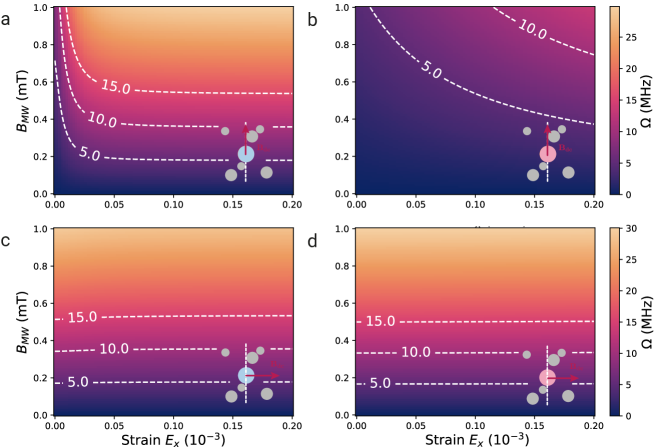
Figure 5: Rabi frequency $\Omega$ dependence on Strain component $E_{x}$ (and $\epsilon_{xy}=0$) and microwave field strength for SiV (a, c) and SnV (b, d). (a, b) depict the parallel configuration while (c, d) depict the perpendicular configuration with $B_{\rm dc}=100$ mT.

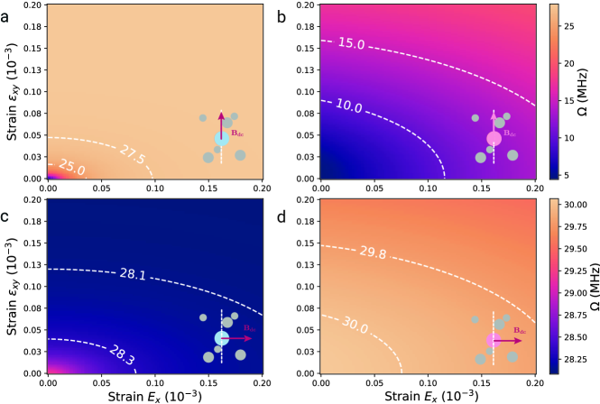
Figure 6: Rabi Frequency $\Omega$ dependence on Strain contributions $E_{x}$ and $\epsilon_{xy}$ for SiV (a, c) and SnV (b, d). (a, b) depict the parallel configuration while (c, d) depict the perpendicular configuration with $B_{\rm dc}=100$ mT. The highest color axis values for the parallel configuration (a, b) is $\Omega=28$ MHz, which is the lowest value for the perpendicular configuration (c, d).

For the case of ${\bf B}_{\rm dc}$ parallel to the symmetry axis, Fig. 5 shows the dependence of the Rabi frequency $\Omega$ as a function the microwave field strength and the externally applied strain for the SiV and SnV. The strain direction $\epsilon_{xy}$ shows a stronger effect in Fig. 6 due to the factor $2$ in $H_{\rm strain}$ [Eq. (9)].

Remarkably, for the chosen values of $B_{\rm ac}=1$ mT and $B_{\rm dc}=100$ mT as well as zero strain, the SnV exhibits an increased $\Omega_{\rm SnV}=30$ MHz compared to the SiV $\Omega_{\rm SnV}=28.4$ MHz, when ${\bf B}_{\rm dc}$ is perpendicular and ${\bf B}_{\rm ac}$ parallel to the symmetry axis. This configuration allows for more efficient control of the SnV compared to the SiV, which is notable given the contrasting behaviour observed when ${\bf B}_{\rm dc}$ aligns with the symmetry axis.

As has been noted in previous work [20, 21], increasing the Rabi frequency requires increased strain. As predicted by Eq. (20), the Rabi frequency saturates as a function of strain at around $\Omega_{\rm max}=28$ MHz for $B_{\rm ac}=1$ mT and $B_{\rm dc}=100$ mT. Due to the reduced $\lambda$ for the SiV, we observe the same behavior as for the SnV except that Rabi frequency increases faster with more strain and more quickly saturates, as shown in Fig. 5.

Fig. 7 shows the dependence of $\Omega$ on the polar angle of the magnetic field (${\bf B}_{\rm ac}$ is parallel to the symmetry axis). For larger values of strain the system is less sensitive to misalignment of $\theta_{\rm dc}$.

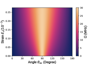
Figure 7: Rabi frequency as a function of $\theta_{\rm dc}$ and Strain component $E_{x}$ ( and $\epsilon_{xy}=0$) with $B_{\rm dc}=100$ mT.

Finally, we numerically calculate microwave qubit gate fidelities for the SiV and SnV. We use an averaged gate fidelity (see for example [39]), which we define as

$$F=\frac{1}{4\pi}\int_{\mathcal{S}}{\rm Tr}(V|\psi\rangle\langle\psi|V^{\dagger}U|\psi\rangle\langle\psi|U^{\dagger})\mathrm{d}\psi$$ (30)

where $V$ is the target gate and $U$ the numerically exact gate, calculated by numerically integrating Schrödingers equation. Here we consider rotations around the x-axis.

In (30), $|\psi\rangle=\cos(\frac{\theta}{2})|1\rangle+e^{{\rm i}\phi}\sin(\frac{\theta}{2})|2\rangle$, for which $\theta\in[0,\pi]$ and $\phi\in[0,2\pi]$. The integral is calculated by integrating over the surface of the Bloch sphere $\mathcal{S}$, using the surface element $\mathrm{d}\psi=\sin(\theta)\mathrm{d}\theta\mathrm{d}\phi$. Gate durations are $\frac{1}{\Omega}$ for a $\pi$ rotation and $\frac{1}{2\Omega}$ for $\pi/2$ rotation. The infidelities $1-F$ for SiV and SnV rotation gates are given in Table 2.

Due to the smaller value of the spin-orbit interaction of the SiV compared to the SnV the qubit splitting $\Delta_{\rm g}^{\rm SiV}$ at zero strain is no longer much smaller than the splitting of the orbital branches, which is required for the approximations leading to Eq. (19). Using the gate duration derived from Eq. (19) therefore leads to slightly decreased gate fidelities. We choose to optimize $B_{ac}$ and therefore the gate duration to minimize the $\pi$ and $\pi/2$ rotation infidelities for the SiV shown in Table 2. We checked, that the addition of strain to the SiV, which increases the splitting of the orbital branches, drastically improved the fidelities without any optimization. Such an optimization was also unnecessary for the SnV, due to the already much larger spin-orbit interaction. In conclusion, Table 2 demonstrates that achievable fidelities are limited only by operational errors and experimental imperfections.

	$B_{\rm ac}$ (mT)	$\Omega$ (MHz)	$T_{\rm\pi/2}$ (ns)	$T_{\rm\pi}$ (ns)	$1-F$
SiV
$B_{dc_{\parallel}}$	1.9	13.3	18.8	37.6	$<10^{-5}$
$B_{dc_{\perp}}$	1.9	56.7	4.4	8.8	$<10^{-4}$
SnV
$B_{dc_{\parallel}}$	1.0	4.4	56.7	113.4	$<10^{-8}$
$B_{dc_{\perp}}$	1.0	30.0	8.3	16.6	$<10^{-10}$

Table 2: Infidely $1-F$ of $\pi/2$ and $\pi$ gate for the SiV and SnV at zero strain and without considering decohering processes and without experimental control imperfections. The values are shown for both configuration (${\bf B}_{dc_{\parallel}}$ and ${\bf B}_{dc_{\perp}}$) for $B_{\rm dc}=100$ mT. $B_{\rm ac}$ is the ac magnetic field strength, $\Omega$ is the Rabi frequency, $T_{\rm\pi/2}$ and $T_{\rm\pi}$ are the duration of $\pi/2$ and $\pi$ rotation around the x-axis on the Bloch sphere, respectively. For both the SiV and SnV $\Delta_{g}\gg 1/\tau_{\rm rad}$ at $B_{\rm dc}>0.1$ T, where $\tau_{\rm rad}>4.5(1.7)$ ns is the radiative lifetime of the SnV [23](SiV [40]).

VI Conclusion & Discussion

In this work we theoretically identified and analysed the most efficient regime for microwave control in the presence of different strain regimes for G4V color centers in diamond. We demonstrated that independent of the specific system parameters of the type of G4V, orienting ${\bf B}_{\rm dc}$ perpendicular to the symmetry axis of the vacancy and driving the system with ${\bf B}_{\rm ac}$ oriented in parallel is the most efficient configuration independent of the magnitude of the strain. This is extremely advantageous for controlling the heavier element color centers such as the SnV and the PbV, which suffer from a bigger penalty in terms of efficiency for a non-perpendicular field orientation of ${\bf B}_{\rm dc}$, requiring higher microwave power, which can potentially increase heating of a sample and have other technical disadvantages. Our analysis also implies that, as far as microwave control is concerned, strain tuning is not necessarily required, greatly reducing experimental overheads.

In conclusion we presented a novel and highly efficient path for controlling G4V independent of strain and the spin-orbit coupling that is compatible with all the required quantum information processing builing blocks, such as initialization, coherent control, and readout.

Author Contributions

M.B compiled the model and performed the comprehensive numerical analysis of the interplay between strain and magnetic field orientations, gate fidelities, initialization and readout. G.P. performed the analytical analysis of the microwave driving as well as the initialization and readout. T.S. and G.P developed the idea and supervised the project. All authors contributed to the writing of the manuscript.

Appendix A Derivation of effective Hamiltonian

After the adiabatic elimination the effective Hamiltonian becomes

$$H_{\rm eff}=H_{\rm B_{\rm dc}}^{\rm eff}+H^{\rm eff}_{\rm B_{\rm ac}(t)}$$ (31)

where

$$\begin{aligned} H_{\rm B}^{\rm eff}=&\gamma_{s}[\Phi(B_{x},B_{y})\sigma_{x}+\Phi(-B_{y},B_{x})\sigma_{y}+\Theta(B_{z})\sigma_{z}]\end{aligned}$$ (32)

$$\begin{aligned} &\Phi(B_{x},B_{y})=\frac{1}{\xi^{2}}\left(B_{x}\upsilon_{y}^{2}+B_{y}\upsilon_{y}\lambda\vphantom{\frac{A}{B}}\right.\\ &\hskip 71.13188pt\left.+\frac{\lambda\upsilon_{x}}{\sqrt{\lambda^{2}+\xi^{2}}}(-\upsilon_{y}B_{y}+\lambda B_{x})\right)\leavevmode\nobreak\ ,\end{aligned}$$ (33)

$$\Theta(B_{z})=-B_{z}\left(\frac{\lambda f\gamma_{l}}{\gamma_{s}\sqrt{\lambda^{2}+\xi^{2}}}+1\right)\leavevmode\nobreak\$$ (34)

where $\sigma_{i}$ are the Pauli matrices. To understand the interplay of strain and microwave control we express the above Hamiltonian in terms of the energy eigenstates of $H_{\rm B_{\rm dc}}^{\rm eff}$. Finally, we can express $H_{\rm B_{\rm ac}(t)}$ in terms of the new eigenbasis to calculate the effective Hamiltonian in Eq. (14) for which we introduce ${\bf B}_{\rm\perp,dc}=(B_{x,\rm dc},B_{y,\rm dc})$. The interaction with the time dependent magnetic field in Eq. (14) is then mediated by

$$\hat{\bm{\mu}}=\begin{pmatrix}\mu_{xx}&\mu_{xy}&\mu_{xz}\\ \mu_{yx}&\mu_{yy}&\mu_{yz}\\ \mu_{zx}&\mu_{zy}&\mu_{zz}\end{pmatrix}\leavevmode\nobreak\ ,$$ (35)

$$\mu_{xx} =4\gamma_{s}^{2}\sin(x)\frac{B_{x,\rm dc}\Theta(B_{z,\rm dc})}{B_{\perp,\rm dc}\Delta_{g}}\leavevmode\nobreak\ ,$$ (36)

$$\mu_{yx} =2\gamma_{s}\sin(x)\frac{B_{y,\rm dc}}{B_{\perp,\rm dc}}\leavevmode\nobreak\ ,$$ (37)

$$\mu_{zx} =4\gamma_{s}\sin(x)^{2}\frac{B_{x,\rm dc}}{\Delta_{g}}\leavevmode\nobreak\ ,$$ (38)

$$\mu_{xy} =\frac{B_{y,\rm dc}}{B_{x,\rm dc}}\mu_{xx}\leavevmode\nobreak\ ,$$ (39)

$$\mu_{yy} =-\frac{B_{x,\rm dc}}{B_{y,\rm dc}}\mu_{yx}\leavevmode\nobreak\ ,$$ (40)

$$\mu_{zy} =\frac{B_{y,\rm dc}}{B_{x,\rm dc}}\mu_{zx}\leavevmode\nobreak\ ,$$ (41)

$$\mu_{xz} =-4\gamma_{s}\sin(x)\frac{B_{\perp,\rm dc}\Theta(B_{z,\rm dc})}{B_{z,\rm dc}\Delta_{g}}\leavevmode\nobreak\ ,$$ (42)

$$\mu_{yz} =0\leavevmode\nobreak\ ,$$ (43)

$$\mu_{zz} =4\gamma_{s}^{2}\frac{\Theta(B_{z,\rm dc})^{2}}{B_{z,\rm dc}\Delta_{g}}$$ (44)

Appendix B Rotating Wave Approximation

$$H_{\rm eff}=-\frac{\Delta_{g}}{2}\sigma_{z}-{\bf S}\cdot\hat{\bm{\mu}}\cdot{\bf B}_{\rm ac}(t)\leavevmode\nobreak\ .$$ (45)

The first term in equation 45 is the free evolution of the system. We can eliminate this term in a rotating frame defined by the transformation

$$|\tilde{\Psi}\rangle =U|\Psi\rangle,$$ (46)

$$U =e^{-i\frac{\Delta_{g}}{2}t\sigma_{z}}.$$ (47)

The new Hamiltonian in this rotating frame is then given by

$$\tilde{H}=UH_{\rm eff}U^{{\dagger}}-iU\dot{U}^{{\dagger}}$$ (48)

In the rotating frame the Hamiltonian becomes

$$\tilde{H}=b(t)\begin{pmatrix}0&\tilde{\Omega}\left(1+e^{-2i\Delta_{g}t}\right)\\ \tilde{\Omega}^{*}\left(1+e^{2i\Delta_{g}t}\right)&0\end{pmatrix}\leavevmode\nobreak\ ,$$ (49)

where rotating wave approximation states entails neglecting the terms $e^{\pm 2i\Delta_{g}t}$, which is justified as long as $\Delta_{g}$ is greater than any other energy scale in the system. In Eq. (49) the complex $\tilde{\Omega}$ can be inferred from Eq. (17).

Appendix C Efficient control

The two functions $f(\phi,\theta_{\rm ac},\theta_{\rm dc})$ and $g(\phi,\theta_{\rm dc},\theta_{\rm ac})$ can be found by taking the respective limits $\lim{\Lambda}_{x\rightarrow 0,\pi/2}$. We find

$$f(\phi,\theta_{\rm dc},\theta_{\rm ac}) =\sqrt{\begin{aligned} &\sin(\phi)^{2}\sin(\theta_{\rm ac})^{2}+\\ &[\cos(\phi)\sin(\theta_{\rm ac})-\cos(\theta_{\rm ac})\tan(\theta_{\rm dc})]^{2}\end{aligned}}$$ (50)

$$g(\phi,\theta_{\rm dc},\theta_{\rm ac}) =\sqrt{\Xi(\phi,\theta_{\rm ac})^{2}+\chi(\phi,\theta_{\rm dc},\theta_{\rm ac})^{2}}$$ (51)

Appendix D Electron-phonon interaction

The thermal phonon bath in diamond interacts with the color center and causes decay and decoherence. This interaction can be modeled by interpreting phonons as dynamical strains deformations [41]

$$H_{\rm e-p}=dE_{x}L_{E_{x}}+2d\epsilon_{xy}L_{\epsilon_{xy}}\leavevmode\nobreak\ ,$$ (52)

where $E_{x}$ and $\epsilon_{xy}$ are now dynamical fields. $L_{E_{x}}=|e_{gx}\rangle\langle e_{gx}|-|e_{gy}\rangle\langle e_{gy}|$ and $L_{\epsilon_{xy}}=|e_{gx}\rangle\langle e_{gy}|+|e_{gy}\rangle\langle e_{gx}|$. The operators $L_{E_{x}}$ and $L_{\epsilon_{xy}}$ determine the levels coupled by electron-phonon interaction.

Decay rates due to electron-phonon interaction can be computed using Fermi’s golden rule

$$\gamma_{ij}=2\pi\rho|\langle i|\tilde{L}|j\rangle|^{2}\leavevmode\nobreak\ ,$$ (53)

where $\rho$ is the density of phononic states and $\tilde{L}=\tilde{L}_{E_{x}},\tilde{L}_{\epsilon_{xy}}$ is given by

$$\tilde{L}=P^{\dagger}LP\leavevmode\nobreak\ .$$ (54)

$P$ is a basis transformation, which allows us to restate $L$ in the eigenbasis of $H_{\rm dc}$ appearing in Eq. (1). To compute $\gamma_{\rm init}$ we only need the matrix elements of $\tilde{L}$, because only the ratios between the decay rates enter Eq. (29). When numerically computing $\tilde{L}$ for $\theta_{\rm dc}=90$ deg we find

$$\tilde{L}_{E_{x}} =a(|4\rangle\langle 4|-|2\rangle\langle 2|)+b(|3\rangle\langle 3|-|1\rangle\langle 1|)+ic(|4\rangle\langle 1|+|3\rangle\langle 2|-|1\rangle\langle 4|-|2\rangle\langle 3|),$$ (55)

$$\tilde{L}_{\epsilon_{xy}} =a^{\prime}i(|1\rangle\langle 2|-|2\rangle\langle 1|+|4\rangle\langle 3|-|3\rangle\langle 4|)+b^{\prime}(|1\rangle\langle 3|+|2\rangle\langle 4|+|3\rangle\langle 1|+|4\rangle\langle 2|).$$ (56)

where $a,b\approx 10^{-1}$, $a^{\prime}\approx 10^{-3}$ and $c,b^{\prime}\approx 1$. From these results we conclude that $E_{x}$ ($\epsilon_{xy}$) phonon modes primarily couples orbital levels with opposite (same) spins, while $\epsilon_{xy}$ very weakly couples opposite spin levels of the same orbital branch.

Appendix E Radiative spontaneous emission

Group theory allows us to determine the non-zero matrix elements of the transition dipole moments but not their magnitudes. This was discussed in [24] including the relative magnitudes of the dipole moments quoted as

$$\begin{aligned} p_{x}=&\begin{pmatrix}0&1\\ 1&0\end{pmatrix}\otimes\begin{pmatrix}1&0&0&0\\ 0&1&0&0\\ 0&0&-1&0\\ 0&0&0&-1\\ \end{pmatrix}\end{aligned}$$ (57)

$$\begin{aligned} p_{y}=&\begin{pmatrix}0&1\\ 1&0\end{pmatrix}\otimes\begin{pmatrix}0&0&-1&0\\ 0&0&0&-1\\ -1&0&0&0\\ 0&-1&0&0\\ \end{pmatrix}\end{aligned}$$ (58)

$$\begin{aligned} p_{z}=&2\begin{pmatrix}0&1\\ 1&0\end{pmatrix}\otimes\begin{pmatrix}1&0&0&0\\ 0&1&0&0\\ 0&0&1&0\\ 0&0&0&1\\ \end{pmatrix}\end{aligned}$$ (59)

Based on the Wigner-Weisskopf approximation [42] we find the spontaneous emission rate of G4Vs

$$\gamma_{ij}=\frac{nw^{3}_{ij}(|\langle i|d_{x}|j\rangle|^{2}+|\langle i|d_{y}|j\rangle|^{2}+|\langle i|d_{z}|j\rangle|^{2})}{3\pi\epsilon_{0}\hbar c^{3}}$$ (60)

where $n=2.42$ is the refractive index of diamond, $\epsilon_{0}$ is the vacuum electric permittivity, $w_{ij}$ is the frequency splitting between the two levels $|i\rangle,|j\rangle$, and ${\bf d}=e\alpha(p_{x},p_{y},p_{z})$ is the transition dipole operator, which includes a scaling factor $\alpha$ that we seek to determine.

The total decay rate from the lowest lying excited state can be decomposed into the zero phonon line (ZPL) and phonon sideband emission rates $\gamma_{\rm total}=\gamma_{\rm ZPL}+\gamma_{\rm PSB}$. For the SnV the emission into the ZPL is given by $\gamma_{\rm ZPL}=60\%\gamma_{\rm total}$ [14]. Given the excited state lifetime of SnV, $\tau=4.5$ns [23], we find $\alpha=8.67635\times 10^{-10}$.

Appendix F Rate equations

We calculate the rate equations for the populations in the strong pumping limit starting with the system’s Hamiltonian in the rotating wave approximation, where we neglect contributions from higher lying excited states. The Hamiltonian in rotating frame is

$$H_{\rm RWA}=\begin{pmatrix}0&0&0&0&\Omega\\ 0&\Delta_{1}&0&0&0\\ 0&0&\Delta_{2}&0&0\\ 0&0&0&\Delta_{3}&0\\ \Omega&0&0&0&0\\ \end{pmatrix}$$ (61)

where $\Delta_{i}=E_{i}-\omega_{L}$, $E_{i}$ is the energy of the $i$th eigenstate $|i\rangle$ of the Hamiltonian in Eq. (3) referenced to the energetically lowest lying ground state and $\omega_{L}$ is the pumping laser’s frequency. We only include the energetically lowest lying excited state $|5\rangle$.

The rate equations in the quasi stationary limit generated by this Hamiltonian can be calculated from the master equation in Lindblad form:

$$\dot{\rho}=-\frac{{\rm i}}{\hbar}[H_{\rm RWA},\rho]+\sum_{\alpha}\gamma_{\alpha}\left(L_{\alpha}\rho L_{\alpha}^{\dagger}-\frac{1}{2}\{L^{\dagger}_{\alpha}L_{\alpha},\rho\}\right)\leavevmode\nobreak\ ,$$ (62)

where $\rho$ is the density matrix, the $L_{\alpha}\in\{L_{15},L_{25},L_{35},L_{45},L_{13},L_{23},L_{14},L_{24}\}$ and $L_{ij}=|i\rangle\langle j|$. We can calculate the optical spontaneous emission rates $\gamma_{15},\gamma_{25},\gamma_{35},\gamma_{45}$ using Eq. (60). The calculation of the phononic spontaneous emission rates $\gamma_{13},\gamma_{23},\gamma_{14},\gamma_{24}$ is explained in D.

After evaluating Eq. 62, we can find the rate equations for the quasi stationary state by assuming that $\dot{\rho}_{ij}=0$ for $i\neq j$. We find after eliminating $\rho_{51}$ and $\rho_{15}$, using the previous assumption

$$\dot{\rho_{11}} =\gamma_{13}\rho_{33}+\gamma_{14}\rho_{44}+\gamma_{15}\rho_{55}+\frac{4(\rho_{55}-\rho_{11})\Omega^{2}}{\gamma_{15}+\gamma_{25}+\gamma_{35}+\gamma_{45}}$$ (63)

$$\dot{\rho_{22}} =\gamma_{23}\rho_{33}+\gamma_{24}\rho_{44}+\gamma_{25}\rho_{55}$$ (64)

$$\dot{\rho_{33}} =-(\gamma_{23}+\gamma_{23})\rho_{33}+\gamma_{35}\rho_{55}$$ (65)

$$\dot{\rho_{44}} =-(\gamma_{14}+\gamma_{24})\rho_{44}+\gamma_{45}\rho_{55}$$ (66)

$$\dot{\rho_{55}} =-(\gamma_{15}+\gamma_{25}+\gamma_{35}+\gamma_{45})\rho_{55}+\frac{4(\rho_{11}-\rho_{55})\Omega^{2}}{\gamma_{15}+\gamma_{25}+\gamma_{35}+\gamma_{45}}$$ (67)

We further eliminate $\rho_{33}$ and $\rho_{44}$ by formally integrating Eqs. (65),(66):

$$\rho_{33} =e^{-(\gamma_{13}+\gamma_{23})t}\rho_{\rm 33}(0)+e^{-(\gamma_{23}+\gamma_{23})t}\int_{-\infty}^{t}e^{(\gamma_{13}+\gamma_{23})\tau}\gamma_{35}\rho_{55}(\tau)\mathrm{d}\tau$$ (68)

$$\approx e^{-(\gamma_{13}+\gamma_{23})t}\rho_{\rm 33}(0)+\frac{\gamma_{35}}{\gamma_{13}+\gamma_{23}}\rho_{55}\leavevmode\nobreak\ ,$$ (69)

$$\rho_{44} =e^{-(\gamma_{14}+\gamma_{24})t}\rho_{\rm 44}(0)+e^{-(\gamma_{14}+\gamma_{23})t}\int_{-\infty}^{t}e^{(\gamma_{14}+\gamma_{24})\tau}\gamma_{45}\rho_{55}(\tau)\mathrm{d}\tau$$ (70)

$$\approx e^{-(\gamma_{14}+\gamma_{24})t}\rho_{\rm 44}(0)+\frac{\gamma_{45}}{\gamma_{14}+\gamma_{24}}\rho_{55}\leavevmode\nobreak\ ,$$ (71)

where we assumed that $\rho_{55}(\tau)$ has no memory and is quasi stationary. Inserting the integrated equations back into Eq. (63) allows us to integrate Eqs. (63), (64) and (67). In the limit of strong pumping we find the relevant equations for the populations shown in Eqs.(27) and (28).

References

- Childress and Hanson [2013] L. Childress and R. Hanson, Diamond NV centers for quantum computing and quantum networks, MRS Bulletin 38, 134 (2013).
- Degen et al. [2017] C. L. Degen, F. Reinhard, and P. Cappellaro, Quantum sensing, Rev. Mod. Phys. 89, 035002 (2017).
- Nguyen et al. [2019] C. T. Nguyen, D. D. Sukachev, M. K. Bhaskar, B. Machielse, D. S. Levonian, E. N. Knall, P. Stroganov, C. Chia, M. J. Burek, R. Riedinger, H. Park, M. Lončar, and M. D. Lukin, An integrated nanophotonic quantum register based on silicon-vacancy spins in diamond, Phys. Rev. B 100, 165428 (2019).
- Bhaskar et al. [2020] M. K. Bhaskar, R. Riedinger, B. Machielse, D. S. Levonian, C. T. Nguyen, E. N. Knall, H. Park, D. Englund, M. Lončar, D. D. Sukachev, and M. D. Lukin, Experimental demonstration of memory-enhanced quantum communication, Nature 580, 60 (2020).
- Gambetta et al. [2017] J. M. Gambetta, J. M. Chow, and M. Steffen, Building logical qubits in a superconducting quantum computing system, npj Quantum Inf 3, 1 (2017).
- Shor [1994] P. Shor, Algorithms for quantum computation: discrete logarithms and factoring, Proceedings 35th Annual Symposium on Foundations of Computer Science , 124 (1994).
- Wang et al. [2018] T. Wang, Z. Zhang, L. Xiang, Z. Jia, P. Duan, W. Cai, Z. Gong, Z. Zong, M. Wu, J. Wu, L. Sun, Y. Yin, and G. Guo, The experimental realization of high-fidelity ‘shortcut-to-adiabaticity’ quantum gates in a superconducting Xmon qubit, New J. Phys. 20, 065003 (2018).
- Yoneda et al. [2018] J. Yoneda, K. Takeda, T. Otsuka, T. Nakajima, M. R. Delbecq, G. Allison, T. Honda, T. Kodera, S. Oda, Y. Hoshi, N. Usami, K. M. Itoh, and S. Tarucha, A quantum-dot spin qubit with coherence limited by charge noise and fidelity higher than 99.9%, Nature Nanotech 13, 102 (2018).
- Harty et al. [2014] T. P. Harty, D. T. C. Allcock, C. J. Ballance, L. Guidoni, H. A. Janacek, N. M. Linke, D. N. Stacey, and D. M. Lucas, High-Fidelity Preparation, Gates, Memory, and Readout of a Trapped-Ion Quantum Bit, Phys. Rev. Lett. 113, 220501 (2014).
- Xia et al. [2015] T. Xia, M. Lichtman, K. Maller, A. Carr, M. Piotrowicz, L. Isenhower, and M. Saffman, Randomized Benchmarking of Single-Qubit Gates in a 2D Array of Neutral-Atom Qubits, Phys. Rev. Lett. 114, 100503 (2015).
- Thiering and Gali [2018] G. Thiering and A. Gali, Ab Initio Magneto-Optical Spectrum of Group-IV Vacancy Color Centers in Diamond, Phys. Rev. X 8, 021063 (2018).
- Neu et al. [2011] E. Neu, D. Steinmetz, J. Riedrich-Möller, S. Gsell, M. Fischer, M. Schreck, and C. Becher, Single photon emission from silicon-vacancy colour centres in chemical vapour deposition nano-diamonds on iridium, New J. Phys. 13, 025012 (2011).
- Palyanov et al. [2015] Y. N. Palyanov, I. N. Kupriyanov, Y. M. Borzdov, and N. V. Surovtsev, Germanium: a new catalyst for diamond synthesis and a new optically active impurity in diamond, Sci Rep 5, 14789 (2015).
- Görlitz et al. [2020] J. Görlitz, D. Herrmann, G. Thiering, P. Fuchs, M. Gandil, T. Iwasaki, T. Taniguchi, M. Kieschnick, J. Meijer, M. Hatano, A. Gali, and C. Becher, Spectroscopic investigations of negatively charged tin-vacancy centres in diamond, New J. Phys. 22, 013048 (2020).
- Santori et al. [2010] C. Santori, P. E. Barclay, K. M. C. Fu, R. G. Beausoleil, S. Spillane, and M. Fisch, Nanophotonics for quantum optics using nitrogen-vacancy centers in diamond, Nanotechnology 21, 274008 (2010).
- Sipahigil et al. [2014] A. Sipahigil, K. D. Jahnke, L. J. Rogers, T. Teraji, J. Isoya, A. S. Zibrov, F. Jelezko, and M. D. Lukin, Indistinguishable Photons from Separated Silicon-Vacancy Centers in Diamond, Phys. Rev. Lett. 113, 113602 (2014).
- Rugar et al. [2020] A. E. Rugar, C. Dory, S. Aghaeimeibodi, H. Lu, S. Sun, S. D. Mishra, Z.-X. Shen, N. A. Melosh, and J. Vučković, Narrow-Linewidth Tin-Vacancy Centers in a Diamond Waveguide, ACS Photonics 7, 2356 (2020).
- Bopp et al. [2022] J. M. Bopp, M. Plock, T. Turan, G. Pieplow, S. Burger, and T. Schröder, ’Sawfish’ Photonic Crystal Cavity for Near-Unity Emitter-to-Fiber Interfacing in Quantum Network Applications, arXiv , 2210.04702 (2022).
- Senkalla et al. [2023] K. Senkalla, G. Genov, M. H. Metsch, P. Siyushev, and F. Jelezko, Germanium Vacancy in Diamond Quantum Memory Exceeding 20 ms, arXiv , 2308.09666 (2023).
- Rosenthal et al. [2023] E. I. Rosenthal, C. P. Anderson, H. C. Kleidermacher, A. J. Stein, H. Lee, J. Grzesik, G. Scuri, A. E. Rugar, D. Riedel, S. Aghaeimeibodi, G. H. Ahn, K. Van Gasse, and J. Vučković, Microwave Spin Control of a Tin-Vacancy Qubit in Diamond, Phys. Rev. X 13, 031022 (2023).
- Guo et al. [2023] X. Guo, A. M. Stramma, Z. Li, W. G. Roth, B. Huang, Y. Jin, R. A. Parker, J. A. Martinez, N. Shofer, C. P. Michaels, C. P. Purser, M. H. Appel, E. M. Alexeev, T. Liu, A. C. Ferrari, D. D. Awschalom, N. Delegan, B. Pingault, G. Galli, F. J. Heremans, M. Atatüre, and A. A. High, Microwave-based quantum control and coherence protection of tin-vacancy spin qubits in a strain-tuned diamond membrane heterostructure, arXiv , 2307.11916 (2023).
- Meesala et al. [2018] S. Meesala, Y.-I. Sohn, B. Pingault, L. Shao, H. A. Atikian, J. Holzgrafe, M. Gündoğan, C. Stavrakas, A. Sipahigil, C. Chia, R. Evans, M. J. Burek, M. Zhang, L. Wu, J. L. Pacheco, J. Abraham, E. Bielejec, M. D. Lukin, M. Atatüre, and M. Lončar, Strain engineering of the silicon-vacancy center in diamond, Phys. Rev. B 97, 205444 (2018).
- Trusheim et al. [2020] M. E. Trusheim, B. Pingault, N. H. Wan, M. Gündoğan, L. De Santis, R. Debroux, D. Gangloff, C. Purser, K. C. Chen, M. Walsh, J. J. Rose, J. N. Becker, B. Lienhard, E. Bersin, I. Paradeisanos, G. Wang, D. Lyzwa, A. R.-P. Montblanch, G. Malladi, H. Bakhru, A. C. Ferrari, I. A. Walmsley, M. Atatüre, and D. Englund, Transform-Limited Photons From a Coherent Tin-Vacancy Spin in Diamond, Phys. Rev. Lett. 124, 023602 (2020).
- Hepp [2014] C. Hepp, Electronic structure of the silicon vacancy color center in diamond, doctoral thesis (2014).
- Sumiya et al. [2023] H. Sumiya, F. Sakano, and N. Tatsumi, Distribution of internal strain and fracture strength in various single-crystal diamonds, Diamond and Related Materials 134, 109781 (2023).
- Fisher et al. [2006] D. Fisher, D. J. F. Evans, C. Glover, C. J. Kelly, M. J. Sheehy, and G. C. Summerton, The vacancy as a probe of the strain in type IIa diamonds, Diamond and Related Materials 15, 1636 (2006).
- Willems et al. [2005] B. Willems, L. C. Nistor, C. Ghica, and G. Van Tendeloo, Strain mapping around dislocations in diamond and cBN, physica status solidi (a) 202, 2224 (2005).
- Hepp et al. [2014] C. Hepp, T. Müller, V. Waselowski, J. N. Becker, B. Pingault, H. Sternschulte, D. Steinmüller-Nethl, A. Gali, J. R. Maze, M. Atatüre, and C. Becher, The electronic structure of the silicon vacancy color center in diamond, Phys. Rev. Lett. 112, 036405 (2014).
- Jahnke et al. [2015] K. D. Jahnke, A. Sipahigil, J. M. Binder, M. W. Doherty, M. Metsch, L. J. Rogers, N. B. Manson, M. D. Lukin, and F. Jelezko, Electron–phonon processes of the silicon-vacancy centre in diamond, New J. Phys. 17, 043011 (2015).
- Paulisch et al. [2013] V. Paulisch, R. Han, H. K. Ng, and B.-G. Englert, Beyond adiabatic elimination: A hierarchy of approximations for multi-photon processes, arXiv , 1209.6568 (2013).
- Hamada [2014] M. Hamada, The minimum number of rotations about two axes for constructing an arbitrarily fixed rotation, Royal Society Open Science 1, 140145 (2014).
- Maity et al. [2020] S. Maity, L. Shao, S. Bogdanović, S. Meesala, Y.-I. Sohn, N. Sinclair, B. Pingault, M. Chalupnik, C. Chia, L. Zheng, K. Lai, and M. Lončar, Coherent acoustic control of a single silicon vacancy spin in diamond, Nat Commun 11, 193 (2020).
- Metsch et al. [2019] M. H. Metsch, K. Senkalla, B. Tratzmiller, J. Scheuer, M. Kern, J. Achard, A. Tallaire, M. B. Plenio, P. Siyushev, and F. Jelezko, Initialization and Readout of Nuclear Spins via a Negatively Charged Silicon-Vacancy Center in Diamond, Phys. Rev. Lett. 122, 190503 (2019).
- Lee et al. [2019] J. P. Lee, B. Villa, A. J. Bennett, R. M. Stevenson, D. J. P. Ellis, I. Farrer, D. A. Ritchie, and A. J. Shields, A quantum dot as a source of time-bin entangled multi-photon states, Quantum Sci. Technol. 4, 025011 (2019), publisher: IOP Publishing.
- Rogers et al. [2014] L. J. Rogers, K. D. Jahnke, M. H. Metsch, A. Sipahigil, J. M. Binder, T. Teraji, H. Sumiya, J. Isoya, M. D. Lukin, P. Hemmer, and F. Jelezko, All-Optical Initialization, Readout, and Coherent Preparation of Single Silicon-Vacancy Spins in Diamond, Phys. Rev. Lett. 113, 263602 (2014).
- Li et al. [2015] L. Li, T. Schröder, E. H. Chen, M. Walsh, I. Bayn, J. Goldstein, O. Gaathon, M. E. Trusheim, M. Lu, J. Mower, M. Cotlet, M. L. Markham, D. J. Twitchen, and D. Englund, Coherent spin control of a nanocavity-enhanced qubit in diamond, Nat. Commun 6, 6173 (2015), number: 1 Publisher: Nature Publishing Group.
- Sukachev et al. [2017] D. D. Sukachev, A. Sipahigil, C. T. Nguyen, M. K. Bhaskar, R. E. Evans, F. Jelezko, and M. D. Lukin, Silicon-Vacancy Spin Qubit in Diamond: A Quantum Memory Exceeding 10 ms with Single-Shot State Readout, Phys. Rev. Lett. 119, 223602 (2017).
- Clark et al. [2023] G. Clark, H. Raniwala, M. Koppa, K. Chen, A. Leenheer, M. Zimmermann, M. Dong, L. Li, Y. H. Wen, D. Dominguez, M. Trusheim, G. Gilbert, M. Eichenfield, and D. Englund, Nanoelectromechanical control of spin-photon interfaces in a hybrid quantum system on chip (2023).
- Magesan et al. [2011] E. Magesan, R. Blume-Kohout, and J. Emerson, Gate fidelity fluctuations and quantum process invariants, Phys. Rev. A 84, 012309 (2011).
- Tamarat et al. [2006] P. Tamarat, T. Gaebel, J. R. Rabeau, M. Khan, A. D. Greentree, H. Wilson, L. C. L. Hollenberg, S. Prawer, P. Hemmer, F. Jelezko, and J. Wrachtrup, Stark Shift Control of Single Optical Centers in Diamond, Phys. Rev. Lett. 97, 083002 (2006).
- Lemonde et al. [2018] M.-A. Lemonde, S. Meesala, A. Sipahigil, M. Schuetz, M. Lukin, M. Loncar, and P. Rabl, Phonon Networks with Silicon-Vacancy Centers in Diamond Waveguides, Phys. Rev. Lett. 120, 213603 (2018).
- Weisskopf and Wigner [1930] V. Weisskopf and E. Wigner, Berechnung der natürlichen Linienbreite auf Grund der Diracschen Lichttheorie, Zeitschrift für Physik 63, 54 (1930).