Recovery of damaged information via scrambling in indefinite casual order

Abstract

Scrambling prevents the access to local information with local operators and therefore can be used to protect quantum information from damage caused by local perturbations. Even though partial quantum information can be recovered if the type of the damage is known, the initial target state cannot be completely recovered, because the obtained state is a mixture of the initial state and a maximally mixed state. Here, we demonstrate an improved scheme to recover damaged quantum information via scrambling in indefinite casual order. We can record the type of damage and improve the fidelity of the recovered quantum state with respect to the original one. Moreover, by iterating the schemes, the initial quantum state can be completely retrieved. In addition, we experimentally demonstrate our schemes on the cloud-based quantum computer, named as Quafu. Our work proposes a feasible scheme to protect whole quantum information from damage, which is also compatible with other techniques such as quantum error corrections and entanglement purification protocols.

I Introduction

Quantum scrambling in a chaotic system can be described as the state being randomized with respect to the Haar measure over the entire Hilbert space [1]. In the view of thermalization, different initial states cannot be distinguished with local measurements of the system [2]. This effect was first studied in the dynamics of black holes [3, 1, 2, 4, 5] and has been attracting growing attention for its close relation to quantum chaos and thermalization in isolated quantum many-body systems [6, 7, 8, 9]. Recently, it has been realized in a variety of systems, including nuclear magnetic resonance (NMR) [10], trapped ions [11, 12, 13], and superconducting [14, 14, 15, 16, 17], Moreover, it relates to quantum information theory [18, 19].

Black holes were once considered as a monster only devouring everything. Then, Hawking radiation reveals that black holes will completely evaporate internal information eventually. By assuming that black holes just process and do not destroy information, it has been shown that information cast into black hole can be recovered, by collecting the Hawking radiation more bits of information than its scrambled [3]. To comply with the quantum no-cloning theorem, the scrambling time should be bounded by an order of $\sim S^{2/D}$, where $S$ and $D$ are the entropy and the dimension of system, respectively [1]. Black holes are the fastest scramblers with an infinite dimension, namely, saturating the bound with an order of $\sim\log S$. This conjecture is also supported by other works in Refs. [2, 4, 5].

Since quantum information cast into the black hole will be emitted after scrambling, this mechanism can be used to recover information. In this Hayden-Preskill black hole thought experiment [3], the quantum information theory is used to show that with the early Hawking radiation and the radiation after scrambling, initial information can be recovered. One of the specific recipes is a teleportation-based decoding protocol [20, 21, 13], which is similar to a traversable wormhole. With the knowledge of the black hole dynamics, information can be retrieved through a quantum memory, pre-entangled with the black hole, by collecting the Hawking radiation. However, this protocol actually collects all initial information, both emitted by the Hawking radiation and left in the black hole, which unrealistically requires considerable knowledge of the black hole system.

A recent scheme, proposed by B. Yan et al. [22], reconstructs initial information without a complete knowledge of the radiation. In details, Alice encodes information by scrambling it with the black hole and can recover information through the backward evolution of the black hole dynamics, where the correlations between radiation and the black hole may be damaged in some degree by the attacker, Bob. This scheme helps to protect and retrieve quantum information against the damage. However, there are still two limitations in this protocol: ($i$) A complete retrieval of initial information relies on the knowledge of the type of the damage. ($ii$) The initial quantum state can only be partially obtained as a mixture of the initial state with the maximally mixed state.

In this paper, we propose an improved scheme for recovering damaged quantum information to cope with the problems by applying the scrambling recovery scheme with the quantum effect of the indefinite casual order (ICO) [23]. Here, auxiliary qubits are used to record the type of damage, with which the first problem is resolved. These auxiliary qubits help to improve the fidelity of recovered state with respect to the initial state, which weaken the requirement of the fidelity of encoding when applying quantum error correction codes (QECCs). In particular, for the damage caused by one-qubit projective measurement, there is a measurement-direction-dependent (MDD) scheme to recover the initial state completely. The scheme can also be iterated, which has the potential to recover the initial state completely from all damage. Our methods to recover the damaged information via scrambling is different from the QECCs and have lower requirement of the fidelity than QECCs, and thus can pre-recover the damaged state over the required fidelity of the QECCs. Our work provides a method to record the type of damage and to distill the damaged quantum state, which allows to retrieve initial information versus any damage.

This paper is organized as follows. In Sec. II, information scrambling and the original protocol proposed in Ref. [22] are reviewed. The improved schemes are discussed in Sec. III, and the iterative schemes are discussed in Sec. IV. In Sec. V, the quantum simulations of several schemes are performed on the Quafu on-cloud quantum computer. The conclusion and discussion are given in Sec. VI.

II Preliminaries

II.1 Scrambling and Out-of-Time Correlations

Information scrambling renders that any two different states will be locally indistinguishable [2], due to the chaotic dynamical evolution. It spreads local information and generates entanglement between different particles, which prevents the access to initial information from local measurement. Two states $\rho_{1}$ and $\rho_{2}$ are locally indistinguishable, if the reduced matrix $\rho_{1}^{S}(t)$ and $\rho_{2}^{S}(t)$ of the two states on a sufficient small subsystem $S$ of a $N$-particle system can be arbitrarily close when time $t$ is long enough. More precisely, for any given small parameter $\delta$, there exists a time $t_{0}$ and a dimensionless parameter $\epsilon$, when $t>t_{0}$ and the subsystem size $|S|<\epsilon N$, $\|\rho_{1}^{S}(t)-\rho_{2}^{S}(t)\|<\delta$ with respect to some norm [2]. This property allows thermalization occurring on a subsystem while the whole system is still out of equilibrium, which releases the contradiction between thermal equilibrium and quantum invertibility [2, 14].

For operator scrambling, we define a direct product operator as $\hat{O}=\bigotimes_{i=1}^{N}\hat{o}_{i}$. First, we consider a local operator initially acting only on the first particle as $\hat{O}_{H}(0)=\hat{o}_{1}\otimes\hat{\mathbb{I}}_{\{2,\dots,N\}}$ and then evolving chaotically as

$$\hat{O}_{H}(t)=\hat{U}^{\dagger}(t)\hat{O}\hat{U}(t)=\sum_{l}s_{l}\hat{O}^{(l)},$$ (1)

where $\hat{O}^{(l)}$ is a $l$-weight term acting on $l$ particles. As the time increases, larger weight terms will be involved in the summation of $\hat{O}_{H}(t)$ [14]. This effect can be detected with the OTOCs

$$C(t)=\langle{\hat{O}_{H}^{\dagger}(t)\hat{W}^{\dagger}\hat{O}_{H}(t)\hat{W}}\rangle,$$ (2)

where $\hat{W}$ is assumed to only act on the $N$-th particle, and without loss of generality, $\hat{O}$ and $\hat{W}$ are assumed to be unitary. At an early time, $\hat{O}_{H}(t)$, acts trivially on the $N$-th particle. Thus, they commute with each other, and the OTOCs $C(t)$ approach to 1. However, as the time increases, terms $\hat{O}^{(l)}$ with a larger weight will be involved in the summation (1), which will act non-trivially on the $N$-th particle. Then, $\hat{O}_{H}(t)$ does not commute with $\hat{W}$, leading to a decay of $C(t)$ from 1.

II.2 Original Recovery Protocol via Scrambling

In the original recovery protocol via scrambling as proposed in Ref. [22], Alice encodes the state of the target system into a black hole, by performing a chaotic evolution of the whole system to fast scramble local information. Then, the target system is exposed to the attacker Bob, who performs some perturbation $\Lambda$ on it, e.g., a projective measurement. After the attack, Alice decodes the target system by backward evolving the whole system. Then, she can retrieve the initial quantum state partially. This procedure is described by the quantum circuit in Fig. 1. The initial state is assumed as $\rho_{\textrm{tb}}^{\textrm{in}}=\rho_{\textrm{t}}\otimes\rho_{\textrm{b}}$, with $\rho_{\textrm{t}}$ and $\rho_{\textrm{b}}$ being the density matrices of the target system (t) and the bath (b), respectively.

For a long-time evolution, the chaotic dynamics can be described as random unitary evolutions uniformly under the Haar measure on the unitary transformation group [4, 22, 24]. This protocol can be understood as a twirling channel in the quantum reference frame theory [18], i.e., the perturbation $\Lambda$ (quantum operation) is twirled by the random unitary transformations $\mathcal{U}(\bullet)=\hat{U}\bullet\hat{U}^{\dagger}$, and the output state of the total system as

$$\rho_{\textrm{tb}}^{\textrm{out}}=\Lambda_{\mathrm{twirl}}(\rho^{\textrm{in}}_{\textrm{tb}}) =\int\!\!d\mathcal{U}\;\mathcal{U}\circ\Lambda\circ\mathcal{U}^{\dagger}(\rho^{\textrm{in}}_{\textrm{tb}})$$ (3)

$$=\int\!\!d\hat{U}\;\sum_{k}\hat{U}\hat{M}_{k}^{\dagger}\hat{U}^{\dagger}\rho^{\textrm{in}}_{\textrm{tb}}\hat{U}\hat{M}_{k}\hat{U}^{\dagger},$$ (4)

where $\hat{M}_{k}$ is the Kraus operators of the completely positive and trace preserving (CPTP) perturbation $\Lambda(\bullet)=\sum_{k}\hat{M}_{k}^{\dagger}\bullet\hat{M}_{k}$ with the identity $\sum_{k}\hat{M}_{k}\hat{M}_{k}^{\dagger}=\hat{\mathbb{I}}$. Using Weingarten’s function [25, 26], we have

$$(D^{2}_{\textrm{tb}}-1)\int\!d\hat{U}\;\hat{U}_{m_{1}n_{2}}\hat{U}_{k_{1}l_{1}}^{\ast}\hat{U}_{m_{2}n_{2}}\hat{U}_{k_{2}l_{2}}^{\ast}$$

$$~{}~{}=\delta_{m_{1}k_{1}}\delta_{m_{2}k_{2}}\delta_{n_{1}l_{1}}\delta_{n_{2}l_{2}}+\delta_{m_{1}k_{2}}\delta_{m_{2}k_{1}}\delta_{n_{1}l_{2}}\delta_{n_{2}l_{1}}$$ (5)

$$~{}~{}~{}~{}~{}~{}-(\delta_{m_{1}k_{1}}\delta_{m_{2}k_{2}}\delta_{n_{1}l_{2}}\delta_{n_{2}l_{1}}+\delta_{m_{1}k_{2}}\delta_{m_{2}k_{1}}\delta_{n_{1}l_{1}}\delta_{n_{1}l_{1}})/D_{\textrm{tb}},$$

where $\delta_{mn}$ is Kronecker delta function, and $D_{\textrm{tb}}$ is the dimension of the composited system, combining the target system (t) and the black hole (b). Then, we have

$$\rho_{\textrm{tb}}^{\textrm{out}}=\Lambda_{\mathrm{twirl}}(\rho_{\textrm{tb}}^{\textrm{in}})=p\rho_{\textrm{tb}}^{\textrm{in}}+{(1-p)}\hat{\mathbb{I}}_{\textrm{tb}}/{D}_{\textrm{tb}},$$ (6)

where the recovery rate

$$p=\frac{\sum_{k}|\mathrm{Tr}\hat{M}_{k}|^{2}-1}{D_{\textrm{tb}}^{2}-1}$$ (7)

is determined by the type of the perturbation $\Lambda$. The output state of the target system can be written as

$$\rho^{\textrm{out}}_{\textrm{t}}=p\rho_{\textrm{t}}+{(1-p)}\hat{\mathbb{I}}_{\textrm{t}}/{D}_{\textrm{t}},$$ (8)

with $D_{\textrm{t}}$ being the dimension of the target system. By performing quantum state tomography (QST) on the target system, Alice can retrieve quantum information of $\rho$ from the damage with the knowledge of $p$. For example, consider a measurement on target qubit (${D}_{\textrm{t}}=2$) with $\hat{M}_{\pm\bm{k}}=({\hat{\mathbb{I}}\pm\bm{k}\cdot\bm{\sigma}})/{2}$, where $\bm{k}=(k_{x},k_{y},k_{z})$ is the measurement direction, and $\bm{\sigma}=(\hat{\sigma}^{x},\hat{\sigma}^{y},\hat{\sigma}^{z})$ with $\hat{\sigma}^{x,y,z}$ being Pauli operators. For $D_{\textrm{tb}}\rightarrow\infty$ (e.g., a black hole), we have

$$p=\frac{D_{\textrm{tb}}^{2}/2-1}{D_{\textrm{tb}}^{2}-1}\rightarrow\frac{1}{2},$$ (9)

indicating that Alice can recover initial quantum information with a recover rate $p=1/2$.

In addition, note that the recovery rate $p$ is related to the average fidelity of the perturbed state with initial states from the Haar ensemble. The average fidelity is expressed as

$$\bar{F}(\Lambda) =\int\!\!d\mathcal{U}\;\mathrm{Tr}[\mathcal{U}(\rho_{\textrm{tb}}^{\textrm{in}})\Lambda\circ\mathcal{U}(\rho_{\textrm{tb}}^{\textrm{in}})]$$

$$=\mathrm{Tr}\left[\rho_{\textrm{tb}}^{\textrm{in}}\int\!\!d\mathcal{U}\;\mathcal{U}^{\dagger}\circ\Lambda\circ\mathcal{U}(\rho_{\textrm{tb}}^{\textrm{in}})\right]$$

$$=\mathrm{Tr}\left[\rho_{\textrm{tb}}^{\textrm{in}}\left(p\rho_{\textrm{tb}}^{\textrm{in}}+{(1-p)}\hat{\mathbb{I}}_{\textrm{tb}}/{D}_{\textrm{tb}},\right)\right]$$

$$=(1-1/{D}_{\textrm{tb}})p+1/{D}_{\textrm{tb}},$$ (10)

where $\rho_{\textrm{tb}}^{\textrm{in}}$ is chosen as a pure state.

Figure 1: Quantum circuit (using qubits as an example) for the original protocol for recovering damaged information via scrambling, where $q_{\textrm{t}}$ is target system, $q_{1},\dots,q_{N}$ denote the bath (black hole).

II.3 Limitations of the Original Recovery Protocol

Before going ahead, we make some assumptions of our schemes in the black hole story. First, we cannot monitor or detect the state of black hole directly. Second, we do not know quantum information that we want to protect. Thus, useful schemes should work for arbitrary initial state of the composited system.

Then, we discuss the problems mentioned in the Introduction. First, $p$ cannot be directly obtained from the QST measurement on the output state, when $\rho$ is a mixed state. Thus, we need to record the recovery rate $p$ given different kinds of damage, which cannot be realized in the original protocol. Second, the output state (8) is a mixture of $\rho_{\textrm{t}}$ with a probability $p$ and $\hat{\mathbb{I}}_{\textrm{t}}/D_{\textrm{t}}$ with $(1-p)$.

Moreover, when the target system has a ${D}_{\textrm{t}}>2$ dimension (e.g., a qudit with ${D}_{\textrm{t}}=4$), and the perturbation is assumed to be a projective measurement, the probability is calculated as

$$p=\frac{\sum_{k}|\mathrm{Tr}\hat{M}_{k}|^{2}-1}{D_{\textrm{tb}}^{2}-1}=\frac{D_{\textrm{tb}}^{2}/{D}_{\textrm{t}}-1}{{D}_{\textrm{t}}^{2}-1}\rightarrow\frac{1}{{D}_{\textrm{t}}},$$ (11)

which means that much less initial information can be recovered using the original protocol in Ref. [22]. Thus, for a target system with a large dimension, we will need to distill information of the initial state $\rho_{\textrm{t}}$ from the mixture (8) to overcome this problem.

II.4 Recovery Assisted by Quantum Error Correction Codes

As the twirling channel of scrambling behaves as a depolarizing channel for the target system, QECCs can be used to protect information. Here, we discuss this problem in the viewpoint of the entanglement purification protocol (EPP). The EPP with one-way classical channels is equivalent to the QECC [27, 28].

The simplest way to demonstrate this equivalence is to use the Choi-Jamiołkowsky (CJ) isomorphism. For any CPTP map $\mathcal{E}:A\rightarrow B$ from a system $A$ to a system $B$, there corresponds to a Choi matrix of the composited system $AB$

$$J_{E}^{AB}=\mathcal{I}\otimes\mathcal{E}(\ket{\phi^{+}}\bra{\phi^{+}}),$$ (12)

where $\ket{\phi^{+}}=\sum_{j=1}^{d_{A}}\ket{j}_{A}\ket{j}_{A^{\prime}}$ is the maximal entangled state of system $A$ and its copy $A^{\prime}$ up to the normalization. The output state of the map $\mathcal{E}$ applied on the state $\rho$ is given as

$$\mathcal{E}(\rho)=\mathrm{Tr}_{A}[J_{E}^{AB}(\rho^{T}\otimes\hat{\mathbb{I}}_{B})].$$ (13)

It establishes the isomorphism between maps $A\rightarrow B$, and the density matrix of the composited system $AB$ up to the normalization, where $A$ is the input system and $B$ is the output system.

Thus, in the qubits system, the Bell state $\ket{\Phi^{+}}=(\ket{00}+\ket{11})/{\sqrt{2}}$ corresponds to the identical channel $\mathcal{I}$, which agrees with the teleportation protocol, and the non-maximal entangled state corresponds to the error channel $\mathcal{E}$. In this circumstance, EPP’s consuming some copies of non-maximal entangled state to distill maximal entangled state is similar as the fact that QECC’s encoding logic qubit into several physical qubits to defend errors. However, for the causality of time, the input state should not be influenced by the output state, thus the EPP, with only one-way classical channel, is equivalent to QECC. One can also construct an EPP from a QECC by applying the transformation $\hat{U}_{E}^{T}$ of encoding operator $\hat{U}_{E}$ on the input system $A$, and the decoding operator $\hat{U}_{D}$ on the output system $B$.

Here, the Choi matrix of scrambling $\Lambda_{\mathrm{t}}$ corresponds to the entangled state

$$\rho_{\textrm{W}}(p)=p\ket{\Phi^{+}}\bra{\Phi^{+}}+(1-p){\hat{\mathbb{I}}}/{4},$$ (14)

which is a Werner state [28], and the fidelity of scrambling of one-qubit measurement lies in $F_{1}={1}/{2}\leq F<F_{\infty}={5}/{8}$. There are lots of purification protocols designed for the Werner state. For the $2\rightarrow 1$ protocol, BBPSSW [29] and DEJMPS [30] protocols require the fidelity $F>{1}/{2}$ of $\ket{\Phi^{+}}$ with the Werner state, while for $M\rightarrow N$ protocols, breeding protocols works only for $F\gtrapprox 0.81$ [29, 28]. When the encoding and decoding operations are not ideal, the minimal required fidelity will increase while the maximal reachable fidelity will decrease, and at some threshold of error rate, the protocol will fail. The BBPSSW and DEJMPS protocols cannot distill the state $\ket{\Phi^{+}}$, if the two-qubit gate fidelities are less that about $0.975$ and $0.965$, and will totally fail if two-qubit gate fidelities are less than $0.965$ and $0.945$ [31]. For a target system with a higher dimension, the minimal required fidelity of QECCs or EPPs is not satisfied even for ideal encoding. Therefore, we need to find other methods to increase the fidelity $F=({1+3p})/{4}$ or equivalently the recovery rate $p$ of the recovered state for the scrambling recovery of the damaged information.

III Improved Scrambling Recovery Schemes

In this section, we discuss two improved schemes and their combination. In the first scheme, the recovery rate $p$, depending on the type of unknown damage, is recorded with an additional qubit. This allows for retrieving all initial information from any damage by performing QST on the target system. Meanwhile, the auxiliary qubit also helps to distill the initial state from the recovered mixed state, which weakens the requirement of two-qubit gate fidelity when applying QECCs. Second, for the projective measurement as the perturbation, it is possible to recover the initial state with a considerably high accuracy. Since the successful probabilities of these schemes are not less than $1/2$, all the advantages mentioned above have practical potential applications.

III.1 Indefinite Casual Order Scheme of Scrambling Recovery

Figure 2: Quantum circuit for the indefinite casual order (ICO) scheme for scrambling recovery of information.

Indefinite casual order (ICO) is a quantum superposition of different sequences of events with different order, which emerges as quantum effect [23]. Two identical fully depolarizing channels or thermalizing channels performed in ICO will preserve the information of the initial state, which cannot be protected in the classic casual order [32, 33]. Therefore, by performing information scrambling in ICO, we can recover more information than the original protocol [22]. The circuit of the quantum-SWITCH of scrambling is shown Fig. 2.

Here, $q_{\textrm{c}}$ is a control qubit, $\hat{U}$ denotes the random unitary operator, and $\Lambda$ is the perturbation channel. The quantum-SWITCH channel is written as

$$\mathcal{V}(\rho_{\textrm{ctb}})=\hat{V}\rho_{\textrm{ctb}}\hat{V}^{\dagger},$$ (15)

where

$$\hat{V}={|0\rangle}_{\textrm{c}}{\langle 0|}\otimes\hat{U}+{|1\rangle}_{\textrm{c}}{\langle 1|}\otimes\hat{U}^{\dagger}.$$ (16)

The quantum twirling channel of the perturbation $\Lambda(\bullet)=\sum_{k}\hat{M}_{k}^{\dagger}\bullet\hat{M}_{k}$ is

$$\Lambda_{\mathrm{twirl}}(\rho_{\textrm{ctb}})=\mathcal{V}\circ\Lambda\circ\mathcal{V}^{-1}(\rho_{\textrm{ctb}})=\sum_{k}\hat{W}_{k}^{\dagger}\rho_{\textrm{ctb}}\hat{W}_{k},$$ (17)

with

$$\hat{W}_{k}=|0\rangle_{\textrm{c}}\langle 0|\otimes\hat{U}\hat{M}_{k}\hat{U}^{\dagger}+{|1\rangle}_{\textrm{c}}\langle{1}|\otimes\hat{U}^{\dagger}\hat{M}_{k}\hat{U}.$$ (18)

Given the input state $\rho^{\mathrm{in}}_{\textrm{ctb}}=|+\rangle_{\textrm{c}}\langle+|\otimes\rho_{\textrm{tb}}^{\textrm{in}}$, the output of the quantum twirling channel is

$$\begin{split}\rho^{\mathrm{out}}_{\textrm{ctb}}=\Lambda_{\mathrm{twirl}}(\rho^{\mathrm{in}}_{\textrm{ctb}})=&\frac{1}{2}\sum_{k}\left[|{0}\rangle_{\textrm{c}}\langle{0}|\otimes\hat{U}\hat{M}_{k}^{\dagger}\hat{U}^{\dagger}\rho_{\textrm{tb}}^{\textrm{in}}\hat{U}\hat{M}_{k}\hat{U}^{\dagger}+|{0}\rangle_{\textrm{c}}\langle{1}|\otimes\hat{U}\hat{M}_{k}^{\dagger}\hat{U}^{\dagger}\rho_{\textrm{tb}}^{\textrm{in}}\hat{U}^{\dagger}\hat{M}_{k}\hat{U}\right.\\ &+\left.|{1}\rangle_{\textrm{c}}\langle{0}|\otimes U^{\dagger}M_{k}U^{\dagger}\rho_{\textrm{tb}}^{\textrm{in}}UM_{k}U^{\dagger}+|{1}\rangle_{\textrm{c}}\langle{1}|\otimes\hat{U}^{\dagger}\hat{M}_{k}^{\dagger}\hat{U}\rho_{\textrm{tb}}^{\textrm{in}}\hat{U}^{\dagger}\hat{M}_{k}\hat{U}\right].\end{split}$$ (19)

Using Eq. (5), we have

$$\rho^{\mathrm{out}}_{\textrm{ctb}}=\hat{\mathbb{I}}_{c}\otimes[p\rho_{\textrm{tb}}^{\textrm{in}}+(1-p)\hat{\mathbb{I}}_{\textrm{tb}}/D_{\textrm{tb}}]/2+\hat{\sigma}_{c}^{x}\otimes\tilde{\rho}_{\textrm{tb}}/2,$$ (20)

where $p=({\sum_{k}|\mathrm{Tr}\hat{M}_{k}|^{2}-1})/({D_{\textrm{tb}}^{2}-1})$, and the density matrix in the second term is

$$\tilde{\rho}_{\textrm{tb}}= \left(p+\frac{1}{D_{\textrm{tb}}^{2}-1}\right)\rho_{\textrm{tb}}^{\textrm{in}}+\frac{1}{D_{\textrm{tb}}^{2}-1}\sum_{k}\hat{M}_{k}^{\dagger}\rho_{\textrm{tb}}^{\textrm{in}}\hat{M}_{k}$$

$$- \frac{1}{D_{\textrm{tb}}(D_{\textrm{tb}}^{2}-1)}\sum_{k}[\mathrm{Tr}(\hat{M}_{k})\rho_{\textrm{tb}}^{\textrm{in}}\hat{M}_{k}^{\dagger}+\mathrm{Tr}(\hat{M}_{k}^{\dagger})\hat{M}_{k}\rho_{\textrm{tb}}^{\textrm{in}}].$$ (21)

Here, we assume the large dimension limit $D_{\textrm{tb}}\rightarrow\infty$. The output state is asymptotically obtained as (see Appendix A)

$$\rho^{\mathrm{out}}_{\textrm{ctb}}\rightarrow\hat{\mathbb{I}}_{\textrm{c}}\otimes[p\rho^{\textrm{in}}_{\textrm{tb}}+(1-p)\hat{\mathbb{I}}_{\textrm{tb}}/D_{\textrm{tb}}]/2+\hat{\sigma}_{\textrm{c}}^{x}\otimes p\rho^{\textrm{in}}_{\textrm{tb}}/2.$$ (22)

By tracing out the bath, we obtain that

$$\rho^{\mathrm{out}}_{\textrm{ct}}\rightarrow\hat{\mathbb{I}}_{\textrm{c}}\otimes[p\rho^{\textrm{in}}_{\textrm{t}}+(1-p)\hat{\mathbb{I}}_{\textrm{t}}/D_{\textrm{t}}]/2+\hat{\sigma}_{\textrm{c}}^{x}\otimes p\rho^{\textrm{in}}_{\textrm{t}}/2.$$ (23)

Since the reduced density matrix of $q_{\textrm{c}}$ can be written as $\rho^{\mathrm{out}}_{\textrm{c}}=(\hat{\mathbb{I}}_{\textrm{c}}+p\hat{\sigma}_{\textrm{c}}^{x})/2$, by measuring the expectation $\langle\hat{\sigma}_{\textrm{c}}^{x}\rangle=p$ on the control qubit, we can obtain exactly the recovery rate $p$, which resolve the first problem. Then, for the measurement in the basis of $|\pm\rangle_{\textrm{c}}$, the post-selected states are

$$\rho^{+}_{\textrm{t}}=\frac{2p}{1+p}\rho^{\textrm{in}}_{\textrm{t}}+\frac{1-p}{1+p}\frac{\hat{\mathbb{I}}_{\textrm{t}}}{D_{\textrm{t}}},$$ (24)

and $\rho^{-}_{\textrm{t}}={\hat{\mathbb{I}}_{\textrm{t}}}/{D_{\textrm{t}}}$, when the outcomes are $\pm$ with probabilities $p_{\pm}=(1\pm p)/2$, respectively. Thus, by post-selecting the state $\rho^{+}$ with respect to the outcome $+$, we can distill the ratio of the initial state in the mixture from a recovery rate $p$ to

$$p_{\textrm{ICO}}=2p/(1+p)\geq p,$$ (25)

with a successful probability $p_{+}=({1+p})/{2}$.

Therefore, this scheme, by performing the scrambling procedure in ICO with a control qubit, can record the damage and improve the fidelity of recovered state. Moreover, it does not require any information of the initial state of the bath qubits and even works without bath qubits.

III.2 Measurement-direction-dependent (MDD) Scheme of Scrambling Recovery

Then, we discuss a special and considerable case, in which the damage by Bob on the target qubit are assumed to be measurements with operators $\{\hat{\Pi}_{s}\}$ with $\sum_{s}\hat{\Pi}_{s}^{\dagger}\hat{\Pi}_{s}=\hat{\mathbb{I}}$ and outcomes $s=\pm 1$. For this case, we can propose a measurement-direction-dependent (MDD) scheme that could completely recover the initial state of the target system for some measurement direction. The circuit of the MDD scheme is shown in Fig. 3, where an accilary qubit, $q_{\textrm{a}}$, is used to detect the direction of the measurement. Here, $\hat{U}$ is the random unitary operator, and the state after the measurement with a outcome $s=$ would be expressed as $\rho_{\textrm{atb}}^{(s)}=\hat{\Pi}_{s}^{\dagger}\rho_{\textrm{atb}}\hat{\Pi}_{s}/p_{s}$, for the outcome with a probability $p_{s}=\textrm{Tr}[\hat{\Pi}_{s}^{\dagger}\rho_{\textrm{atb}}\hat{\Pi}_{s}]$, where $\bm{r}=(r_{x},r_{y},r_{z})$ is the direction of the projective measurement.

Then, the output state is

$$\rho^{(s)}_{\textrm{atb}}= \Lambda_{\mathrm{twirl}}(\rho^{\mathrm{in}}_{\textrm{atb}})=\frac{1}{2}|0\rangle_{\textrm{a}}\langle 0|\otimes\rho^{(s)}_{\textrm{tb1}}+\frac{1}{2}|0\rangle_{\textrm{a}}\langle{1}|\otimes\rho^{(s)}_{\textrm{tb2}}$$

$$+\frac{1}{2}|{1}\rangle_{\textrm{a}}\langle{0}|\otimes\rho^{(s)}_{\textrm{tb3}}+\frac{1}{2}|{1}\rangle_{\textrm{a}}\langle 1|\otimes\rho^{(s)}_{\textrm{tb4}},$$ (26)

where

$$\rho_{\textrm{tb1}}^{(s)}\propto\int\!\!d\hat{U}\;\hat{U}^{\dagger}\hat{\Pi}_{s}^{\dagger}\hat{U}\rho^{\textrm{in}}_{\textrm{tb}}\hat{U}^{\dagger}\hat{\Pi}_{s}\hat{U},$$ (27a)

$$\rho_{\textrm{tb2}}^{(s)}\propto\int\!\!d\hat{U}\;\hat{U}^{\dagger}\hat{\Pi}_{s}^{\dagger}\hat{U}\rho^{\textrm{in}}_{\textrm{tb}}\hat{U}^{\dagger}\hat{\sigma}_{\textrm{t}}^{x}\hat{U}\hat{\Pi}_{s}\hat{\sigma}_{\textrm{t}}^{x}\hat{U},$$ (27b)

$$\rho_{\textrm{tb3}}^{(s)}\propto\int\!\!d\hat{U}\;\hat{U}^{\dagger}\hat{\sigma}_{\textrm{t}}^{x}\hat{\Pi}_{s}^{\dagger}\hat{\sigma}_{\textrm{t}}^{x}\hat{U}\rho^{\textrm{in}}_{\textrm{tb}}\hat{U}^{\dagger}\hat{\Pi}_{s}\hat{U},$$ (27c)

$$\rho_{\textrm{tb4}}^{(s)}\propto\int\!\!d\hat{U}\;\hat{U}^{\dagger}\hat{\sigma}_{\textrm{t}}^{x}\hat{\Pi}_{s}^{\dagger}\hat{\sigma}_{\textrm{t}}^{x}\hat{U}\rho^{\textrm{in}}_{\textrm{tb}}\hat{U}^{\dagger}\hat{\sigma}_{\textrm{t}}^{x}\hat{\Pi}_{s}\hat{\sigma}_{1}^{x}\hat{U}.$$ (27d)

Applying Eq. (5) (see Appendix B for more details), we obtain that

$$\rho_{\textrm{tb1}}^{(s)}=\rho_{\textrm{tb4}}^{(s)}=\frac{1}{2}[p\rho^{\textrm{in}}_{\textrm{tb}}+(1-p){\hat{\mathbb{I}}_{\textrm{tb}}}/{D_{\textrm{tb}}}],$$ (28a)

$$\rho_{\textrm{tb2}}^{(s)}=\rho_{\textrm{tb3}}^{(s)}=\frac{1}{2}[{p}^{\prime}\rho^{\textrm{in}}_{\textrm{tb}}+(r_{x}^{2}-{p}^{\prime}){\hat{\mathbb{I}}_{\textrm{tb}}}/{D_{\textrm{tb}}}],$$ (28b)

where

$${p}^{\prime}=\frac{D_{\textrm{tb}}^{2}/2-r_{x}^{2}}{D_{\textrm{tb}}^{2}-1}\rightarrow p\rightarrow\frac{1}{2},~{}\textrm{for}~{}D_{\textrm{tb}}\rightarrow\infty.$$

In the large dimension limit $D_{\textrm{tb}}\rightarrow\infty$, the output state with respect to the outcome $s$ can be written as

$$\rho^{(s)}_{\textrm{atb}}\rightarrow \hat{\mathbb{I}}_{\textrm{a}}\otimes[p\rho^{\textrm{in}}_{\textrm{tb}}+(1-p){\hat{\mathbb{I}}_{\textrm{tb}}}/{D_{\textrm{tb}}}]/2$$

$$+\hat{\sigma}_{\textrm{a}}^{x}\otimes[p\rho^{\textrm{in}}_{\textrm{tb}}+\left(r_{x}^{2}-p\right){\hat{\mathbb{I}}_{\textrm{tb}}}/{D_{\textrm{tb}}}]/2,$$ (29)

and the corresponding probability $p_{s}=\frac{1}{2}$. Note that the output state is independent of the outcome $s$ of the projective measurement, which hereafter is omitted.

Figure 3: Quantum circuit for the measurement-direction-dependent (MDD) scheme for scrambling recovery of information.

By measuring the auxiliary qubit $q_{\textrm{a}}$ in the $\ket{\pm}_{\textrm{a}}$ basis, we could obtain

$$\rho^{+}_{\textrm{tb}}=\frac{2p}{1+r_{x}^{2}}\rho^{\textrm{in}}_{\textrm{tb}}+\left(1-\frac{2p}{1+r_{x}^{2}}\right)\frac{\hat{\mathbb{I}}_{\textrm{tb}}}{D_{\textrm{tb}}},$$ (30)

with a successful conditional probability $p_{+|s}=({1+r_{x}^{2}})/{2}$, and $\rho^{-}_{\textrm{tb}}=\hat{\mathbb{I}}_{\textrm{tb}}/D_{\textrm{tb}}$ with a failing conditional probability $p_{-|s}=({1-r_{x}^{2}})/{2}$. Thus, the squred $x$-component of the measurement $r_{x}^{2}$ can be estimated by measuring the auxiliary qubit in the $\ket{\pm}_{\textrm{a}}$ basis. Furthermore, by post-selecting the state $\rho^{+}_{\textrm{tb}}$ with respect to the outcome $+$, the recovery ratio is improved to

$$p_{\textrm{MDD}}={2p}/({1+r_{x}^{2}})\geq p,$$ (31)

with $0\leq r_{x}^{2}\leq 1$, and the output state of the target system is

$$\rho^{+}_{\textrm{t}}=\frac{2p}{1+r_{x}^{2}}\rho^{\textrm{in}}_{\textrm{t}}+\left(1-\frac{2p}{1+r_{x}^{2}}\right)\frac{\hat{\mathbb{I}}_{\textrm{t}}}{D_{\textrm{t}}}$$ (32)

Surprisingly, if $r_{x}=0$, i.e., the direction of the measurement is in the $y$-$z$ plane, with $p={1}/{2}$, we have $p_{\textrm{MDD}}=1$, which indicates a complete recovery of the initial state.

Figure 4: Quantum circuit for the combination of the ICO and MDD schemes.

We also consider the case that the measurement is not in a fixed direction, e.g., the attacker perform measurement in random directions $r_{x}=\sin\theta$, with $\theta$ being uniformly distributed in the range $[0,2\pi]$. We can obtain the average $\overline{r_{x}^{2}}=1/2$, and the recovery ratio is $\bar{p}_{\textrm{MDD}}=2/3$, with a average successful probability $\bar{p}_{+}=3/4$, which is same as the ICO scheme.

In summary, for a direction-fixed measurement, the MDD scheme can record the squared $x$-component of the measurement $r_{x}^{2}$, which allows us to optimize the scheme to completely recover initial quantum information of the target system. Even for the measurements in random directions, it behaves as good as the ICO scheme.

III.3 Combination of Indefinite Casual Order (ICO) and Measurement-Direction-Dependent (MDD) Schemes

The above two schemes are different: The ICO scheme requires a control qubit manipulating the forwards and backwards evolutions, and the MDD scheme requires an ancillary qubit detecting the measurements on the target system. Thus, it is possible to combine these two schemes, of which the quantum circuit is shown in Fig. 4.

After the post-section with respect to the outcome $+_{\textrm{c}}+_{\textrm{a}}$ of the control qubit and the ancillary qubit, the final state of the target system can calculated as

$$\rho^{++}_{\textrm{t}}=\frac{4p}{1+r_{x}^{2}+2p}\rho^{\textrm{in}}_{\textrm{t}}+\left(1-\frac{4p}{1+r_{x}^{2}+2p}\right)\frac{\hat{\mathbb{I}}_{\textrm{t}}}{D_{\textrm{t}}},$$ (33)

with a successful probability $p_{++}=({1+r_{x}^{2}})/{4}+{p}/{2}$. The ratio $p_{\textrm{co}}$ of recovered information is

$$p_{\textrm{co}}=\frac{4p}{1+r_{x}^{2}+2p}\geq\frac{2p}{1+p},$$ (34)

which is larger than either the ICO scheme or the MDD scheme. In addition, when $r_{x}=0$ with $p={1}/{2}$, we obtain that $p_{\textrm{co}}=1$, which means the merit of total recovery is inherited successfully. Similarly, for the case that the measurement direction randomly chosen, the average recovery ratio is $\bar{p}_{\textrm{co}}={4}/{5}$, with an average successful probability $\bar{p}_{++}={5}/{8}$. These results show that these the ICO and MDD schemes are well compatible with each other.

IV Iterative Scrambling Recovery Schemes

Next, we discuss iterative scrambling recovery schemes, which improve the fidelity between the initial state and the recovered state. For the scrambling recovery of the target system with $D_{\textrm{t}}$ dimension, the recover rate $p$ scales as $\sim D_{\textrm{t}}^{-l}$, where $l$ depends on the types of the perturbations on target system. It is possible to improve the recovery rate close to $1$ exponentially with an increasing number of iterations. However, the errors, occurring during the scrambling procedure, will ruin a complete recovery of initial information, which is similar to the EPP. Fortunately, the scrambling recovery schemes are compatible with QECC or EPP.

Figure 5: The circuit of iterative scrambling protocol.

IV.1 Iterative Scrambling Recovery Protocol

The random evolutions, applied on the same target system and bath several times directly, are not effective to iterate the scrambling recovery protocol. The reason is that the evolution is random with Haar measure, which is invariant under the group multiplication of unitary evolution group $U(2^{N})$. Thus, no matter how many layers of scrambling are applied, it is equivalent to a single layer of scrambling. The solution to this problem is to scramble the target system with different baths, the circuit is shown in Fig. 5.

We consider a $n$-iterated twirling channel $\Lambda^{(n)}$ with the perturbation $\Lambda$ acting on target system and set $\Lambda^{(0)}\equiv\Lambda$. For $n\geq 1$, the twirling channel $\Lambda^{(n-1)}$ can be regarded as a depolarizing channel with a depolarized rate $1-p^{(n-1)}$, which can be written as

$$\Lambda^{(n-1)}(\rho_{\textrm{t}})=p^{(n-1)}\rho_{\textrm{t}}+(1-p^{(n-1})\mathrm{Tr}(\rho_{\textrm{t}})\hat{\mathbb{I}}_{\textrm{t}}/D_{\textrm{t}}$$ (35)

$$=\frac{(D_{\textrm{t}}^{2}-1)p^{(n-1)}+1}{D_{\textrm{t}}^{2}}\hat{U}_{0}\rho\hat{U}_{0}^{\dagger}+\frac{1-p^{(n-1)}}{D_{\textrm{t}}^{2}}\sum_{i\neq 0}\hat{U}_{i}\rho_{\textrm{t}}\hat{U}_{i}^{\dagger},$$

where $\{\hat{U}_{i}\}$ are the orthogonal unitary operator bases acting on the target system, which satisfy $\hat{U}_{0}=\hat{\mathbb{I}}_{\textrm{t}}$, and $\mathrm{Tr}(\hat{U}_{i}^{\dagger}\hat{U}_{j})=D_{\textrm{t}}\delta_{ij}$, for $i=0,1,\dots,D_{\textrm{t}}^{2}-1$. Then the depolarized rate of $\Lambda_{n}$ satisfies

$$1-p^{(n)}=\frac{1-1/D_{\textrm{t}}^{2}}{1-1/D_{\textrm{tb}}^{2}}(1-p^{(n-1)}).$$ (36)

When the dimension $D_{\textrm{t}}$ of the target system is clearly smaller than dimension $D_{\textrm{tb}}$ of total scrambled system, ${(1-1/D_{\textrm{t}}^{2})}/{(1-1/D_{\textrm{tb}}^{2})}<1$, the depolarized rate of depolarizing channel is suppressed after scrambling. Thus, we get

$$\rho^{(n)}_{\textrm{t}}=p^{(n)}\rho^{\textrm{in}}_{\textrm{t}}+(1-p^{(n)})\hat{\mathbb{I}}_{\textrm{t}}/D_{\textrm{t}}\rightarrow\rho^{\textrm{in}}_{\textrm{t}},$$ (37)

with the recover ratios being written as

$$p^{(n)}=1-(1-p)\left(\frac{1-1/D_{\textrm{t}}^{2}}{1-1/D_{\textrm{tb}}^{2}}\right)^{n-1}\!\!\!\rightarrow 1,$$ (38)

where $p=({\sum_{k}|\mathrm{Tr}\hat{M}_{k}|^{2}-1})/({D_{\textrm{tb}}^{2}-1})$ is determined by perturbation $\Lambda$. Thus, the output target state shows that the $n$-th iterated twirling channel can perform a complete recovery of quantum information of the target system. The imperfection of scrambling will affect the performance of this scheme, see Appendix C.1 for more details.

Note that this convergence is independent of the initial recover ratio $p$ decided by the form of the perturbation and is thus robust. The reason is that Eq. (36) is a first order equation, which has only one attractive fixed point when $D_{\textrm{t}}<D_{\textrm{tb}}$. Thus, although the error in scrambling will lower the fixed point of recovery rate, there is no threshold, which is different from the EPP or QECC. Here, we also remark that this scheme requires at least one bath qubit in each step of iteration, otherwise $D_{\textrm{t}}=D_{\textrm{tb}}$, and any ratio $p$ is the fixed point. Thus, the number of baths will increase with iterations, which decides the performance of the recovery of initial quantum information .

IV.2 Iterative Indefinite Casual Order Scheme

Figure 6: Quantum circuit for the asymptotic iterative ICO-scrambling scheme.

Figure 7: Quantum circuit for the exact iterative ICO-scrambling scheme.

For the iterative ICO-scrambling scheme, we add $n$ control qubits, $q_{\textrm{c}_{1}},q_{\textrm{c}_{2}},q_{\textrm{c}_{3}},\cdots,q_{\textrm{c}_{n}}$, that manuplating the forward or backwards random evolution. The circuit of this scheme is shown in Fig. 6.

In the limit $D_{\textrm{tb}}\rightarrow\infty$, after post-selecting the state with respect to the outcome $+$ of the control qubit, the first ICO-twirling channel $\Lambda^{(1)}_{\textrm{ICO}}$ behaves as a depolarizing channel acting on the target system and the bath with a depolarized rate $(1-p^{(1)}_{\textrm{ICO}})$, where

$$p^{(1)}_{\textrm{ICO}}=\frac{2p}{1+p},$$ (39)

and $p$ is the recovery rate of the original perturbation $\Lambda^{(0)}_{\textrm{ICO}}\equiv\Lambda$ for the scrambling procedure. Then, we can assume that the $n-1$-th ICO-twirling channel $\Lambda^{(n-1)}_{\textrm{ICO}}$ also behaves as a depolarizing channel on target system and bath with a depolarized rate $(1-p^{(n-1)}_{\textrm{ICO}})$ as

$$\Lambda^{(n-1)}_{\textrm{ICO}}(\rho_{\textrm{tb}})=p^{(n-1)}_{\textrm{ICO}}\rho_{\textrm{tb}}+(1-p^{(n-1)}_{\textrm{ICO}})\mathrm{Tr}(\rho_{\textrm{tb}})\hat{\mathbb{I}}_{\textrm{tb}}/D_{\textrm{tb}}$$ (40)

$$=\frac{(D_{\textrm{tb}}^{2}-1)p^{(n-1)}_{\textrm{ICO}}+1}{D_{\textrm{tb}}^{2}}\hat{U}_{0}\rho_{\textrm{tb}}\hat{U}_{0}^{\dagger}+\frac{1-p^{(n-1)}_{\textrm{ICO}}}{D_{\textrm{tb}}^{2}}\sum_{i\neq 0}\hat{U}_{i}\rho_{\textrm{tb}}\hat{U}_{i}^{\dagger},$$

where $\{\hat{U}_{i}\}$ are orthogonal unitary operator bases acting on the target system and the bath, with $\hat{U}_{0}=\hat{\mathbb{I}}_{\textrm{tb}}$ and $\mathrm{Tr}(\hat{U}_{i}^{\dagger}\hat{U}_{j})=D_{\textrm{tb}}\delta_{ij}$, for $i=0,1,\dots,D_{\textrm{tb}}^{2}-1$. Then, the recovery rate of the $n$-th iterative ICO-scrambling scheme can be obtained as

$$p^{(n)}_{\textrm{ICO}}=\frac{2^{n}p}{(2^{n}-1)p+1}\rightarrow 1,$$ (41)

from the recursive formula

$$p^{(n)}_{\textrm{ICO}}=\frac{2p^{(n-1)}_{\textrm{ICO}}}{1+p^{(n-1)}_{\textrm{ICO}}}.$$ (42)

Therefore, the output state of the target system after the post-selection for the $n$-th iterative ICO scheme can be written as

$$\rho^{(n)}_{\textrm{t}}=\Lambda^{(n)}_{\textrm{ICO}}(\rho_{\textrm{t}}^{\textrm{in}})=p^{(n)}_{\textrm{ICO}}\rho^{\textrm{in}}_{\textrm{t}}+(1-p^{(n)}_{\textrm{ICO}})\hat{\mathbb{I}}_{\textrm{t}}/D_{\textrm{t}}\rightarrow\rho^{\textrm{in}}_{\textrm{t}},$$ (43)

indicating a complete recovery of initial information.

However, when the dimension of the bath is not infinite large, the side effect in the thermodynamic limit cannot be neglected. Thus, the iterative ICO-twirling channel constructed in Fig. 6 cannot be taken as a depolarizing channel. To overcome this problem, we first twirl the perturbation $\Lambda$ by scrambling it with the bath without using ICO, which is labelled as $\Lambda^{(0)}\equiv\Lambda_{\mathrm{twirl}}$ and can be expressed by a depolarization channel on the target system and the bath with a depolarizing rate $(1-p)$, as shown in Eq. (8). This exact iterative ICO-scrambling scheme is shown in Fig. 7. Then, we can obtain the $n-1$-th ICO-twirling channel as a depolarizing channel in Eq. (40) for a finite size of the bath, and the output state of the $n$-th ICO-twirling channel is given using Eq. (20) and Eq. (III.1) as

$$\rho^{(n)}_{\textrm{ctb}}= \ \hat{\mathbb{I}}_{c}\otimes[p_{\textrm{eICO}}^{(n-1)}\rho_{\textrm{tb}}^{\textrm{in}}+(1-p_{\textrm{eICO}}^{(n-1)})\hat{\mathbb{I}}_{\textrm{tb}}/D_{\textrm{tb}}]/2$$

$$+\hat{\sigma}_{c}^{x}\otimes\tilde{\rho}^{(n)}_{\textrm{tb}}/2,$$ (44)

$$\tilde{\rho}_{\textrm{tb}}^{(n)}= \left[p_{\textrm{eICO}}^{(n-1)}+\frac{D_{\textrm{tb}}^{2}-2}{D_{\textrm{tb}}^{2}(D_{\textrm{tb}}^{2}-1)}(1-p_{\textrm{eICO}}^{(n-1)})\right]\rho_{\textrm{tb}}^{\textrm{in}}$$

$$+\frac{1-p^{(n-1)}}{D_{\textrm{tb}}^{2}-1}\frac{\hat{\mathbb{I}}}{D_{\textrm{tb}}}.$$ (45)

By finally post-selecting the outcome of the control qubit $q_{\textrm{c}_{n}}$ as $+$ with a successful probability

$$p_{+}=\frac{1+p_{\textrm{eICO}}^{(n-1)}}{2}+\frac{1-p_{\textrm{eICO}}^{(n-1)}}{D^{2}_{\textrm{tb}}},$$ (46)

the output state can also be expressed as a density matrix through a depolarization channel as

$$\Lambda^{(n)}_{\textrm{eICO}}(\rho_{\textrm{t}})=p_{\textrm{eICO}}^{(n)}\rho_{\textrm{t}}^{\textrm{in}}+(1-p_{\textrm{eICO}}^{(n)})\frac{\hat{\mathbb{I}}_{\textrm{t}}}{D_{\textrm{t}}},$$ (47)

where

$$p_{\textrm{eICO}}^{(n)}=\frac{2p_{\textrm{eICO}}^{(n-1)}+\frac{D_{\textrm{tb}}^{2}-2}{D_{\textrm{tb}}^{2}(D_{\textrm{tb}}^{2}-1)}(1-p_{\textrm{eICO}}^{(n-1)})}{1+p_{\textrm{eICO}}^{(n-1)}+\frac{2}{D_{\textrm{tb}}^{2}}(1-p_{\textrm{eICO}}^{(n-1)})}.$$ (48)

This recursive formula has an attractive fixed point at $p_{1}^{(\infty)}=1$ and an unstable fixed point at $p_{2}^{(\infty)}=-{1}/({D_{\textrm{tb}}^{2}-1})$. Thus, the initial state can be recovered completely for the scrambling recovery scheme for any perturbation with a recovery rate $p>0$. In the vicinity of $p_{1}^{(\infty)}=1$, the recursive equation up to first order is written as

$$(p_{\textrm{eICO}}^{(n)}-1)=\frac{1}{2}\left[1+\frac{1}{2(D_{\textrm{tb}}^{2}-1)}\right](p_{\textrm{eICO}}^{(n-1)}-1),$$ (49)

where the coefficient

$$\frac{1}{2}\left[1+\frac{1}{2(D_{\textrm{tb}}^{2}-1)}\right]\leq\frac{5}{8}$$ (50)

for $D_{\textrm{tb}}\geq 2$. While for iterative scheme without using ICO, the coefficient of linear order

$$\frac{1-1/D_{\textrm{t}}^{2}}{1-1/D_{\textrm{tb}}^{2}}\geq\frac{3}{4}\left(\frac{D_{\textrm{tb}}^{2}}{D_{\textrm{tb}}^{2}-1}\right)\geq\frac{3}{4},$$ (51)

which means that the convergence of the iterative ICO-scrambling scheme to $1$ is faster than the standard iterative scrambling protocol for a larger $D_{\textrm{tb}}$.

The influence of the noise of the control qubits on this scheme is discussed in Appendix C.2. It is shown that the iterative ICO-scrambling scheme is robust with a recovery rate $p$ for scrambling the perturbation, and the performance depends on the number of control qubits, while the bath can be used repeatedly. The iterative ICO-scrambling schemes is also more efficient than the standard iterative scrambling recovery protocol. However, since the fixed point equation of the iterative ICO-scrambling scheme is second-order, the robustness of this scheme has a threshold behavior according to the noise.

V Quantum simulation of Scrambling Recovery Schemes with On-Cloud superconducting Processor

Figure 8: Quantum circuit for the $2$-design twirling channel.

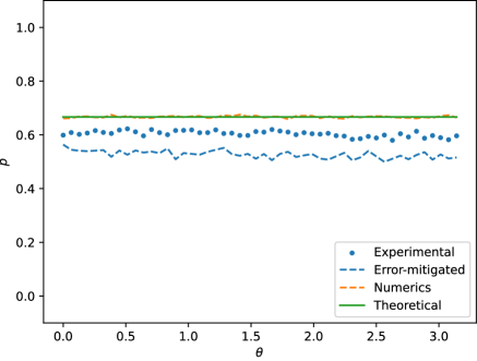
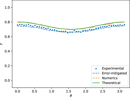
Figure 9: LABEL:sub@subfig:_design_ico Quantum circuit for the ICO-scrambling recovery scheme via using the $2$-design. The probe qubit $q_{\textrm{p}}$ is used to perform the perturbative measurement on the target qubit $q_{\textrm{t}}$. The quantum circuit is performed in each element of Clifford group with $1,000$ shots, and the measurement angle $\theta$ is chosen in the range $[0,\pi]$ as $50$ equal spacing points. LABEL:sub@subfig:_trace The recovery ratio $p=\langle\hat{\sigma}_{\textrm{c}}^{x}\rangle$ versus the measurement angle $\theta$. LABEL:sub@subfig:_fidelity_ico Fidelity of the recovered state with the initial state $F$ versus $\theta$.

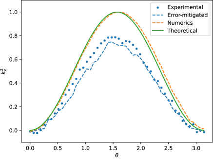
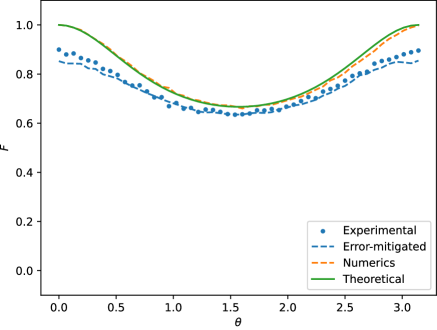
Figure 10: LABEL:sub@subfig:_design_direction Quantum circuit for the MDD-scrambling recovery scheme with the $2$-design. The probe qubit $q_{\textrm{p}}$ is used to perform the perturbative measurement on the target qubit $q_{\textrm{t}}$. The quantum circuit is performed in each element of Clifford group with $1,000$ shots, and the measurement angle $\theta$ is chosen in the range $[0,\pi]$ as $50$ equal spacing points. LABEL:sub@subfig:_direction The $x$-component of the squared projective measurement $r_{x}^{2}=\langle\hat{\sigma}_{\textrm{a}}^{x}\rangle$ versus the measurement angle $\theta$. LABEL:sub@subfig:_fidelity Fidelity of the recovered state with the initial state versus $\theta$.

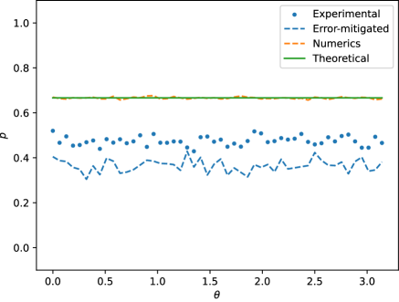
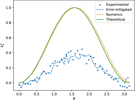
(a) Direction of perturbative measurement

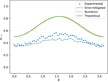
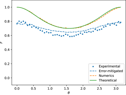
Figure 11: LABEL:sub@subfig:_design_ico Quantum circuit for the combination of the ICO- and MDD-scrambling schemes with th $2$-design. The probe qubit $q_{\textrm{p}}$ is used to perform the perturbative measurement on the target qubit $q_{\textrm{t}}$. The quantum circuit is performed in each element of the Clifford group with $1,000$ shots, and the measurement angle $\theta$ is chosen in the range $[0,\pi]$ as $50$ equally spacing points. LABEL:sub@subfig:_trace_ico_d Recovery rate $p=\langle\hat{\sigma}_{\textrm{c}}^{x}\rangle$ versus the measurement angle $\theta$. LABEL:sub@subfig:_r_x^2_ico_d The curve of direction $r_{x}^{2}=\langle\hat{\sigma}_{\textrm{a}}^{x}\rangle$ versus $\theta$. LABEL:sub@subfig:_q_ico_d Sucessful probability for the post-selection $p_{++}$ versus $\theta$. LABEL:sub@subfig:_fidelity_ico Fidelity of the recovered state with the initial state versus $\theta$.

The realization of a random unitary evolution with Haar measure is of great importance in information scrambling. However, to realize this randomness requires many layers of quantum gates, which is limited by the coherent time in the noisy intermediate-scale quantum (NISQ) era. Thus, a direct experimental realization of the randomness is not easy in state-of-art experimental technique.

One way to preserve the property of randomness and to reduce the complexity of the quantum circuit simultaneously is to use the unitary $t$-design [34]. For the twirling channel, we need at least to apply the $2$-design, and fortunately, the Clifford group, widely used in error bench-marking of quantum gates, satisfies this requirement (see Appendix D for more details). Here, we design the circuit of the twirling channel as shown in Fig. 8, where $\Gamma_{i}$ is an element of the Clifford group, and $\sum_{i}$ represents the average on Clifford group.

With this circuit, we can simulate our improved recovery schemes on a NISQ quantum processor. Since the Clifford group of $2$ qubits has $11,520$ elements and is hard to realize, only the schemes without bath, namely the ICO- and MDD-scrambling schemes, are simulated. The quantum circuits are performed on the Quafu on-cloud quantum computers [35], of which the experimentally results are compared to both theoretical predictions and numerical calculations.

V.1 Quantum Simulation of the ICO-scrambling Scheme

The quantum circuit is shown in Fig. 9, where $q_{\textrm{c}}$ is a control qubit, $q_{\textrm{t}}$ is the target qubit, and $q_{\textrm{p}}$ is the probe qubit used to perform the perturbative measurement. Here, $Y(\theta)$ denotes the rotation operators with an angle $\theta$ along $y$-axis, which determines the direction of the measurement. The initial state of the target system is prepared as $\ket{0_{z}}$. When averaging over the Clifford group, the quantum circuit is equivalent to averaging the ones with initial states congruent to $\ket{0_{z}}$ up to the Clifford group, e.g., $\ket{0_{x}}and\ket{0_{y}}$.

The results are shown in Fig. 9. Figure 9 shows that the expectation $\langle\hat{\sigma}_{\textrm{c}}^{x}\rangle$ of the control qubit $q_{\textrm{c}}$, representing the coherent part of the reduced density matrix of $q_{\textrm{c}}$, is invariant versus the direction $\theta$. In Fig. 9, we show the fidelity versus the measurement direction $\theta$. Note that the fidelity varies for different measurement directions, which is different from the theoretical prediction in the previous discussions. This is because that the thermodynamic limit $D_{\textrm{tb}}\rightarrow\infty$ is not saturated, and the side effect that we have neglected accounts for the dependency of the fidelity on the measurement direction. The theoretical prediction, considering the side effect (see Appendix E.1.1) is plotted as the solid curve in Fig. 9, which coincides with the numerical calculation.

The experimental results fit well with our theoretical prediction and numerical calculation even with some errors. The error-mitigated theoretical results are shown using the blue dashed curve in Fig. 9 (see Appendix E.2.1 for more details).

V.2 Quantum simulation of the MDD-scrambling Scheme

The quantum circuit is shown in Fig. 10, where $q_{\textrm{a}}$ is an auxiliary qubit, $q_{\textrm{t}}$ is the target qubit, and $q_{\textrm{p}}$ is the probe qubit. The initial state of the target system is also prepared as $\ket{0_{z}}$. The direction of measurement, detected by the auxiliary qubit $q_{\textrm{a}}$, is shown in Fig. 10, and the fidelity of the recovered state of $q_{\textrm{t}}$ with initial state is shown in Fig. 10. The numerical calculation coincides with the theoretical prediction, and the experimental results also verifies the dependency of recovery fidelity on the measurement direction, even when the error is considered.

We also show that the error depends on the measurement direction, since only the $Y(\pi)$ gate of the on-cloud quantum processor has been carefully calibrated, while the $Y(\theta)$ gate with an arbitrary rotation angle $\theta$ has not. The error-mitigated theoretical results are shown as the blue dashed curve in Fig. 10 (see Appendix E.2.2 for more details).

V.3 Quantum Simulation of the Combination of the ICO- and MDD-scrambling Schemes

The quantum circuit for the combination of ICO- and MDD- scrambling schemes is shown in Fig. 11, where $q_{\textrm{c}}$ is the control qubit, $q_{\textrm{t}}$ is the target qubit, $q_{\textrm{a}}$ is the auxiliary qubit, and $q_{\textrm{p}}$ is the probe qubit. The results are shown in Fig. 11. Figure 11 plotts the probability $p_{++}$ of the basis $\ket{+}_{\textrm{c}}\otimes\ket{+}_{\textrm{t}}$ on $q_{\textrm{c}}$ and $q_{\textrm{t}}$ for the post-selection. We see that the error between experimental and theoretical results is larger than the combination of the errors of two experiments above. Note that except for the direction dependent error appearing in the quantum simulation of the MDD-scrambling scheme, there is a large error that is independent of the direction. However, this error does not exist in the quantum simulation of the ICO-scrambling scheme, which is much smaller.

The possible origin of this error is from the CNOT gate on $q_{\textrm{t}}$ and $q_{\textrm{p}}$. Since our quantum processor is a qubit chain, $q_{\textrm{p}}$ does not connect $q_{\textrm{t}}$ directly. Thus, to perform this CNOT gate, there require two SWAP gates between $q_{\textrm{a}},q_{\textrm{p}}$, which lead to a large error than the results of previous schemes. The error-mitigated theoretical results are shown as the blue dashed line in Fig. 11 (see Appendix E.2.3 for more details).

VI Conclusion

In this paper, we propose two improved information recovery schemes via scrambling that overcome the problems encountered in the original recovery protocol proposed in Ref. [22]. The ICO-scrambling scheme asymptotically can record information of the damage and promote the fidelity of the recovered state by performing the post-selection. However, it has the side effect when the bath is not large enough. This drawback can be overcome by scrambling the target system without ICO before performing the ICO-scrambling scheme. The MDD-scrambling scheme is designed for the projective measurement perturbation on the qubit target system only. This scheme allows a completely recovery of the initial state, if the measurement direction is fixed in the $y$-$z$ plane. Otherwise, it allows for recording the $x$-component of the measurement. If the measurement direction is not fixed, the average recovery performance of the MDD-scrambling scheme is same as the ICO-scrambling scheme.

In addition, these scrambling recovery schemes can also be iterated, to completely recover the initial state under arbitrary damage. We discuss the iteration of the original recovery protocol [22], and the iterative ICO-scrambling scheme. To iterate the original scrambling recovery protocol would scramble the target system with different baths. Therefore, the iterative ICO-scrambling scheme could exhibit the its advantage that it repeatedly uses a single bath.

These scrambling recovery schemes use redundant qubits to reduce the effects of the damage on the target system, which in fact could be taken as a kind of passive QECs [36]. In comparison, the active QECs can improve the ability to defend the errors by detecting them and performing corrections based on their syndromes, and the types of errors are confined by the stabilizers [37].

Finally, the ICO-scrambling scheme, the MDD-scrambling scheme, and their combination are simulated on the on-cloud quantum computer, Quafu. The experimental results are compared with the theoretical predictions and numerical calculations, which fit well when error is mitigated.

Our results provide methods to record the type of the damage and to distill the damaged quantum state, which allows to retrieve initial information against different types of the damage. We expect that our scheme will be useful in the both quantum information recovery from the damage and system’s bench-marking.

Appendix A Asymptotic Analysis of the recovered state

To analyze the asymptotic behavior of $\tilde{\rho}_{\textrm{tb}}$, we employ the Hilbert-Schmidt inner product $(\hat{A},\hat{B})=\mathrm{Tr}(\hat{A}^{\dagger}\hat{B})$ and the induced norm $\|\hat{A}\|^{2}=\mathrm{Tr}(\hat{A}^{\dagger}\hat{A})$. We have

$$\|\tilde{\rho}_{\textrm{tb}}-p\rho_{\textrm{tb}}^{\textrm{in}}\|\leq \left\|\frac{1}{D_{\textrm{tb}}^{2}-1}\rho_{\textrm{tb}}^{\textrm{in}}\right\|+\left\|\frac{1}{D_{\textrm{tb}}^{2}-1}\sum_{k}\hat{M}_{k}^{\dagger}\rho_{\textrm{tb}}^{\textrm{in}}\hat{M}_{k}\right\|$$ (52)

Precisely, we have

$$\left\|\frac{\rho_{\textrm{tb}}^{\textrm{in}}}{D_{\textrm{tb}}^{2}-1}\right\|^{2}=\frac{\mathrm{Tr}(\rho_{\textrm{tb}}^{\textrm{in}})^{2}}{D_{\textrm{tb}}^{2}-1}\leq\frac{1}{D_{\textrm{tb}}^{2}-1}\rightarrow 0,$$ (54)

$$\left\|\frac{1}{D_{\textrm{tb}}^{2}-1}\sum_{k}\hat{M}_{k}^{\dagger}\rho_{\textrm{tb}}^{\textrm{in}}\hat{M}_{k}\right\|^{2} =\frac{1}{D_{\textrm{tb}}^{2}-1}\mathrm{Tr}\left[\left(\sum_{k}\hat{M}_{k}^{\dagger}\rho_{\textrm{tb}}^{\textrm{in}}\hat{M}_{k}\right)^{2}\right]\leq\frac{1}{D_{\textrm{tb}}^{2}-1}\rightarrow 0,$$ (55)

$$\left\|\frac{1}{D_{\textrm{tb}}(D_{\textrm{tb}}^{2}-1)}\sum_{k}[\mathrm{Tr}(\hat{M}_{k})\rho_{\textrm{tb}}^{\textrm{in}}\hat{M}_{k}^{\dagger}+\mathrm{Tr}(\hat{M}_{k}^{\dagger})\hat{M}_{k}\rho_{\textrm{tb}}^{\textrm{in}}]\right\|$$

$$=\frac{1}{D_{\textrm{tb}}(D_{\textrm{tb}}^{2}-1)}\sum_{k,l}\textrm{Re}[\mathrm{Tr}(\hat{M}_{k})\mathrm{Tr}(\hat{M}_{l})\mathrm{Tr}(\rho_{\textrm{tb}}^{\textrm{in}}\hat{M}_{l}^{\dagger}\rho_{\textrm{tb}}^{\textrm{in}}\hat{M}_{k}^{\dagger})+\mathrm{Tr}(\hat{M}_{k})\mathrm{Tr}(\hat{M}_{l}^{\dagger})\mathrm{Tr}(\hat{M}_{l}\rho^{2}\hat{M}_{k}^{\dagger})]$$

$$\leq\frac{1}{D_{\textrm{tb}}(D_{\textrm{tb}}^{2}-1)}\sum_{k,l}|\mathrm{Tr}(\hat{M}_{k})\mathrm{Tr}(\hat{M}_{l})|\times\left[|\mathrm{Tr}(\rho_{\textrm{tb}}^{\textrm{in}}\hat{M}_{l}^{\dagger}\rho_{\textrm{tb}}^{\textrm{in}}\hat{M}_{k}^{\dagger})|+|\mathrm{Tr}(\hat{M}_{l}(\rho_{\textrm{tb}}^{\textrm{in}})^{2}\hat{M}_{k}^{\dagger})|\right]$$

$$\leq\frac{1}{D_{\textrm{tb}}(D_{\textrm{tb}}^{2}-1)}\left(\sum_{k}|\mathrm{Tr}(\hat{M}_{k})|^{2}\right)\left[\sqrt{\sum_{k,l}|\mathrm{Tr}(\rho_{\textrm{tb}}^{\textrm{in}}\hat{M}_{l}^{\dagger}\rho_{\textrm{tb}}^{\textrm{in}}\hat{M}_{k}^{\dagger})|^{2}}+\sqrt{\sum_{k,l}|\mathrm{Tr}(\hat{M}_{l}(\rho_{\textrm{tb}}^{\textrm{in}})^{2}\hat{M}_{k}^{\dagger})|^{2}}\right].$$ (56)

Then, with the Cauchy-Schwarz inequality on Hilbert-Schmidt inner product, we have

$$\sum_{k}|\mathrm{Tr}(\hat{M}_{k})|^{2} \leq\sum_{k}\mathrm{Tr}(\hat{\mathbb{I}}^{2})\mathrm{Tr}(\hat{M}_{k}^{\dagger}\hat{M}_{k})=D_{\textrm{tb}}^{2},$$ (57)

$$\sum_{k,l}|\mathrm{Tr}(\rho_{\textrm{tb}}^{\textrm{in}}\hat{M}_{l}^{\dagger}\rho_{\textrm{tb}}^{\textrm{in}}\hat{M}_{k}^{\dagger})|^{2} \leq\sum_{k}\mathrm{Tr}(\rho_{\textrm{tb}}^{\textrm{in}}\hat{M}_{k}^{\dagger}\hat{M}_{k}\rho_{\textrm{tb}}^{\textrm{in}})\sum_{k}\mathrm{Tr}[\hat{M}_{k}(\rho_{\textrm{tb}}^{\textrm{in}})^{2}\hat{M}_{k}^{\dagger}]=\mathrm{Tr}^{2}\left(\rho_{\textrm{tb}}^{\textrm{in}}\right)^{2}\leq 1,$$ (58)

$$\sum_{k,l}|\mathrm{Tr}[\hat{M}_{l}(\rho_{\textrm{tb}}^{\textrm{in}})^{2}\hat{M}_{k}^{\dagger}]|^{2} \leq\left[\sum_{k}\mathrm{Tr}(\hat{M}_{k}(\rho_{\textrm{tb}}^{\textrm{in}})^{2}\hat{M}_{k}^{\dagger})\right]^{2}=\mathrm{Tr}^{2}(\rho_{\textrm{tb}}^{\textrm{in}})^{2}\leq 1,$$ (59)

and

$$\left\|\frac{1}{D_{\textrm{tb}}(D_{\textrm{tb}}^{2}-1)}\sum_{k}[\mathrm{Tr}(\hat{M}_{k})\rho_{\textrm{tb}}^{\textrm{in}}\hat{M}_{k}^{\dagger}+\mathrm{Tr}(\hat{M}_{k}^{\dagger})\hat{M}_{k}\rho_{\textrm{tb}}^{\textrm{in}}]\right\| \leq\frac{4}{(D_{\textrm{tb}}^{2}-1)^{2}}\rightarrow 0.$$ (60)

Thus, we conclude that

$$\lim_{D_{\textrm{tb}}\rightarrow\infty}\tilde{\rho}_{\textrm{tb}}=p\rho_{\textrm{tb}}^{\textrm{in}}.$$ (61)

Appendix B Output state of the MDD Scheme

With Eq. (5), we have

$$\rho_{\textrm{tb1}}^{(s)}=\rho_{\textrm{tb4}}^{(s)}\propto \left[\frac{|\mathrm{Tr}\hat{\Pi}_{s}|^{2}}{D_{\textrm{tb}}^{2}-1}-\frac{\mathrm{Tr}(\hat{\Pi}_{s}^{\dagger}\hat{\Pi}_{s})}{D_{\textrm{tb}}(D_{\textrm{tb}}^{2}-1)}\right]\rho^{\textrm{in}}_{\textrm{tb}}+\left[\frac{D_{\textrm{tb}}\mathrm{Tr}(\hat{\Pi}_{s}^{\dagger}\hat{\Pi}_{s})}{D_{\textrm{tb}}^{2}-1}-\frac{|\mathrm{Tr}\hat{\Pi}_{s}|^{2}}{D_{\textrm{tb}}^{2}-1}\right]\frac{\hat{\mathbb{I}}}{D_{\textrm{tb}}}.$$ (62)

$$\rho_{\textrm{tb2}}^{(s)}=\rho_{\textrm{tb3}}^{(s)}\propto \left[\frac{|\mathrm{Tr}\hat{\Pi}_{s}|^{2}}{D_{\textrm{tb}}^{2}-1}-\frac{\mathrm{Tr}(\hat{\Pi}_{s}^{\dagger}\hat{\sigma}_{\textrm{t}}^{x}\hat{\Pi}_{s}\hat{\sigma}_{\textrm{t}}^{x})}{D_{\textrm{tb}}(D_{\textrm{tb}}^{2}-1)}\right]\rho^{\textrm{in}}_{\textrm{tb}}+\left[\frac{D_{\textrm{tb}}\mathrm{Tr}(\hat{\Pi}_{s}^{\dagger}\hat{\sigma}_{\textrm{t}}^{x}\hat{\Pi}_{s}\hat{\sigma}_{\textrm{t}}^{x})}{D_{\textrm{tb}}^{2}-1}-\frac{|\mathrm{Tr}\hat{\Pi}_{s}|^{2}}{D_{\textrm{tb}}^{2}-1}\right]\frac{\hat{\mathbb{I}}}{D_{\textrm{tb}}}.$$ (63)

With $\hat{\Pi}_{s=\pm 1}=({\hat{\mathbb{I}}+s\bm{n}\cdot\bm{\sigma}_{\textrm{t}}})/{2}$,

$$\mathrm{Tr}\left(\hat{\Pi}_{s}^{\dagger}\hat{\Pi}_{s}\right) =\mathrm{Tr}\hat{\Pi}_{s}=\frac{D_{\textrm{tb}}}{2},$$ (64)

$$\mathrm{Tr}(\hat{\Pi}_{s}^{\dagger}\hat{\sigma}_{x}\hat{\Pi}_{s}\hat{\sigma}_{x}) =\mathrm{Tr}\left(\frac{{\hat{\mathbb{I}}+s\bm{r}\cdot\bm{\sigma}_{\textrm{t}}}}{2}\frac{{\hat{\mathbb{I}}+s\bm{r}^{\prime}\cdot\bm{\sigma}_{\textrm{t}}}}{2}\right)=(1+\bm{r}\cdot\bm{r}^{\prime})\frac{D_{\textrm{tb}}}{4}=\frac{r_{x}^{2}D_{\textrm{tb}}}{2},$$ (65)

where $\bm{r}^{\prime}=(r_{x},-r_{y},-r_{z})$ is the vector obtained from $\bm{r}$ by rotating $\pi$ about $x$ direction. Thus, we have

$$\rho_{\textrm{tb1}}^{(s)} =\rho_{\textrm{tb4}}^{(s)}=\frac{1}{2}\left[p\rho^{\textrm{in}}_{\textrm{tb}}+(1-p)\frac{\hat{\mathbb{I}}_{\textrm{tb}}}{D_{\textrm{tb}}}\right],$$ (66)

$$\rho_{\textrm{tb2}}^{(s)} =\rho_{\textrm{tb3}}^{(s)}=\frac{1}{2}\left[p^{\prime}\rho^{\textrm{in}}_{\textrm{tb}}+\left(r_{x}^{2}-p^{\prime}\right)\frac{\hat{\mathbb{I}}_{\textrm{tb}}}{D_{\textrm{tb}}}\right],$$ (67)

where

$$p^{\prime}=2\left[\frac{|\mathrm{Tr}\hat{\Pi}_{s}|^{2}}{D_{\textrm{tb}}^{2}-1}-\frac{\mathrm{Tr}(\hat{\Pi}_{s}^{\dagger}\hat{\sigma}_{\textrm{t}}^{x}\hat{\Pi}_{s}\hat{\sigma}_{\textrm{t}}^{x})}{D_{\textrm{tb}}(D_{\textrm{tb}}^{2}-1)}\right]=\frac{D_{\textrm{tb}}^{2}/2-r_{x}^{2}}{D_{\textrm{tb}}^{2}-1}$$ (68)

Appendix C Noisy Iterative Recovery Schemes

C.1 Noisy Iterative Scrambling Recovery Protocol

In the noisy scrambling protocol, the fixed point of the recursive equation will be influenced by the error occruing during the scrambling procedure. To investigate this case, we plot the noisy iterative quantum circuit in Fig. 12, where the error of scrambling is desribed as $\mathcal{E}(\rho)=\sum_{k}\hat{K}_{k}\rho\hat{K}_{k}^{\dagger}$.

The total noisy perturbation in $n$-th step is written as

$$\tilde{\Lambda}^{(n)}(\rho_{\textrm{t}})= \ \Lambda^{(n)}\circ\mathcal{E}^{(n)}(\rho_{\textrm{t}})$$

$$= \ p^{(n)}\mathcal{E}^{(n)}(\rho_{\textrm{t}})+(1-p^{(n)})\hat{\mathbb{I}}_{\textrm{t}}/D_{\textrm{t}}$$ (69)

$$= \ p^{(n)}\sum_{k}\hat{K}^{(n)}_{k}\rho_{\textrm{t}}{\hat{K}^{(n)\dagger}_{k}}+\frac{1-p^{(n)}}{D_{\textrm{t}}^{2}}\sum_{i}\hat{U}_{i}\rho_{\textrm{t}}\hat{U}_{i}^{\dagger},$$

with a recovery rate

$$p^{(n)}=(x^{(n-1)}-s)p^{(n-1)}+s,$$ (70)

where $s={(D_{\textrm{tb}}^{2}/D_{\textrm{t}}^{2}-1)}/{(D_{\textrm{tb}}^{2}-1)}$, and $(1-x^{(n)})$ is the depolarizing ratio of $\mathcal{E}^{(n)}$ as $\mathcal{E}^{(n)}(\rho)=x^{(n)}\rho+(1-x^{(n)})\hat{\mathbb{I}}/D$. We can view the composition of $\mathcal{E}^{(0)}$ and $\Lambda^{(0)}$ as one effective initial perturbation $\tilde{\Lambda}$. For convenience, we let the error channel be the same $\mathcal{E}^{(l)}=\mathcal{E}$ with $x^{(n)}=x$ and have that

$$p^{(n)}=\frac{s}{s+1-x}-\left(x-s\right)^{n-1}\left(\frac{s}{s+1-x}-\tilde{p}\right),$$ (71)

where $\tilde{p}$ is the ratio of the efficient initial perturbation $\tilde{\Lambda}$. The recursive formula is still a first-order equation, and the stability of the fixed point is determined by whether $|x-s|<1$. If $-(1-s)<x<1$, in the limit $n\rightarrow\infty$, $p^{(n)}\rightarrow{s}/{(s+1-x)}$. Meanwhile, if the dimension of bath goes to infinity, $s\rightarrow{1}/{D_{\textrm{t}}^{2}}$, we obtain that

$$p^{(n)}\rightarrow\frac{1}{1+(1-x)D_{\textrm{t}}^{2}}.$$ (72)

Figure 12: Quantum circuit for the noisy iterative twirling channel.

Thus, $p^{(n)}$ scales as $\sim{1}/{D_{\textrm{t}}^{2}}$, when the error rate $1-x$ is independent of $D_{\textrm{t}}$, which is not better than the original protocol. If the error rate scales as $1-x\sim\alpha D_{\textrm{t}}^{-2}$, the ratio of recovered information is $p^{(\infty)}\sim{1}/{(1+\alpha)}<1$ being a constant. uniform to perturbation $\Lambda$.

C.2 Noisy Iterative ICO-scrambling Scheme

The depolarizing error on the control qubit with an error rate $(1-x)$ transforms the output state as

$$\rho^{\epsilon(n)}_{\textrm{ctb}}=x\rho^{(n)}_{\textrm{ctb}}+(1-x){\hat{\mathbb{I}}_{\textrm{ctb}}}/({D_{\textrm{ctb}}}),$$ (73)

where $\rho^{(n)}_{\textrm{ctb}}$ is shown in Eq. (44) and (45). By performing the post-selection, the recursive equation becomes

$$p_{\textrm{eICO}}^{(n)}=\frac{x\left[2p_{\textrm{eICO}}^{(n-1)}+\frac{D_{\textrm{tb}}^{2}-2}{D_{\textrm{tb}}^{2}(D_{\textrm{tb}}^{2}-1)}(1-p_{\textrm{eICO}}^{(n-1)})\right]}{1+x\left[p_{\textrm{eICO}}^{(n-1)}+\frac{2}{D_{\textrm{tb}}^{2}}(1-p_{\textrm{eICO}}^{(n-1)})\right]}.$$ (74)

It is complex to solve this equation, so we only consider the case $D_{\textrm{tb}}=2$, and the equation is simplified as

$$p_{\textrm{eICO}}^{(n)}=\frac{4x(2p_{\textrm{eICO}}^{(n-1)}+1)}{3\left[2+x(1+p_{\textrm{eICO}}^{(n-1)})\right]},$$ (75)

with a fixed point

$$p_{\textrm{eICO}}^{(\infty)}=\frac{5}{6}-\frac{1}{x}\pm\frac{\sqrt{73x^{2}-60x+36}}{6x}<x,$$ (76)

when $x\in[0,1]$. Thus, the recovery rate scheme is also limited by the error rate on the control qubit.

Appendix D Quantum simulation of Haar randomness with Unitary $t$-design

Unitary $t$-design of Haar measure on a unitary group $U$ is a finite subset $S$, satisfying that

$$\frac{1}{|S|}\sum_{S}f(S,S^{\dagger})=\int\!\!d\hat{U}\;f(\hat{U},\hat{U}^{\dagger}),$$ (77)

where $f(\hat{U},\hat{U}^{\dagger})$ is a homogeneous polynomial with $t$ degree of elements of $\hat{U}$ and also polynomial of elements of $\hat{U}^{\dagger}$.

Using the unitary design with proper $t$, we can mimic the randomness easily. In the case of information scrambling, the random Haar measure is integrated on the so-called twirling channel

$$\Lambda_{t}=\int\!\!d\mathcal{U}\;f(\mathcal{U},\Lambda)=\int\!\!d\mathcal{U}\;\mathcal{U}\circ\Lambda\circ\mathcal{U}^{\dagger},$$ (78)

whose integrand is a polynomial with $2$-degree of $\hat{U}$ and also $\hat{U}^{\dagger}$. So if we average on the unitary $2$-design can mimic the Haar measure theoretically.

Figure 13: Quantum circuit for the approximate scrambling evolution.

The method to mimic the Haar randomness used in the original protocol [22] is the 3-qubit unitary operator

$$\hat{U}=\hat{\mathbb{I}}_{1}\otimes\ket{01}\bra{00}+\hat{\sigma}_{1}^{x}\otimes\ket{00}\bra{01}-\imath\hat{\sigma}_{1}^{y}\otimes\ket{11}\bra{10}-\hat{\sigma}_{1}^{z}\otimes\ket{10}\bra{11},$$ (79)

whose circuit is shown in Fig. 13. Here $q_{1}$ is the working qubit, $q_{2},q_{3}$ are the bath with initial state $\ket{+}$. With this circuit, we can calculate that for any channel $\Lambda$, the corresponding channel twirled by $U$ can send any input of $q_{1}$ with $\rho$ into the state with reduced density matrix on $q_{1}$ as

$$\rho_{\mathrm{twirl}}=\Lambda_{\mathrm{twirl}}(\rho)=\sum_{i}\sum_{k}\hat{\sigma}_{i}\hat{M}_{k}\hat{\sigma}_{i}\rho\hat{\sigma}_{i}\hat{M}_{k}^{\dagger}\hat{\sigma}_{i},$$ (80)

where $\hat{\sigma}_{i}\in P=\{\hat{\mathbb{I}}_{1},\hat{\sigma}_{1}^{x},\hat{\sigma}_{1}^{y},\hat{\sigma}_{1}^{z}\}$ is elements of Pauli group, and $\Lambda(\rho)=\sum_{k}\hat{M}_{k}\rho\hat{M}_{k}^{\dagger}$. For Pauli group is only the unitary $1$-design, this can not mimic the twirling channel only, which has integrated with $2$ degree polynomial. Thus, it also needs one more average of perturbation $\Lambda$ on Pauli group, which prevent us from manipulating the direction of perturbation. Moreover, the 3-qubit unitary is hard to realize when we also want to manipulate its evolution.

Theoretically, this unitary operator is just a realization of average on unitary $1$-design, we can actually average it "by hand" like the average of the direction of perturbation on Pauli group. With this idea, we come back to the average on unitary $t$-design, at less $t=2$, which have a famous one, the Clifford group (table 1), and we arrive the circuit (Fig. 8) in mean text.

Axis	Angle	Realization
		I
$(1,0,0)$	$\pi$	X
$(0,1,0)$	$\pi$	Y
$(0,0,1)$	$\pi$	Z
$(1,0,0)$	$\pi/2$	X/2
$(-1,0,0)$	$\pi/2$	-X/2
$(0,1,0)$	$\pi/2$	Y/2
$(0,-1,0)$	$\pi/2$	-Y/2
$(0,0,1)$	$\pi/2$	-X/2 Y/2 X/2
$(0,0,-1)$	$\pi/2$	-X/2 -Y/2 X/2
$(1,0,1)$	$\pi$	X -Y/2
$(-1,0,1)$	$\pi$	X Y/2
$(0,1,1)$	$\pi$	Y X/2
$(0,-1,1)$	$\pi$	Y -X/2
$(1,1,0)$	$\pi$	X/2 Y/2 X/2
$(1,-1,0)$	$\pi$	-X/2 Y/2 -X/2
$(1,1,1)$	$2\pi/3$	Y/2 X/2
$(-1,1,1)$	$2\pi/3$	Y/2 -X/2
$(1,-1,1)$	$2\pi/3$	-Y/2 X/2
$(-1,-1,1)$	$2\pi/3$	-Y/2 -X/2
$(1,1,1)$	$-2\pi/3$	-X/2 -Y/2
$(-1,1,1)$	$-2\pi/3$	X/2 -Y/2
$(1,-1,1)$	$-2\pi/3$	-X/2 Y/2
$(-1,-1,1)$	$-2\pi/3$	-X/2 -Y/2

Table 1: Twenty-four elements of the Clifford group.

Appendix E Details of Simulation

The experiments are performed on the ScQ-P18 backend of the Quafu platform. The layout of the ScQ-P18 device and the error rates of CZ gates are shown in Fig. 14. The qubits $q_{0},q_{1},q_{2}$ of the circuits in Fig. 9, 10 are mapped to the physical qubits $q_{2},q_{3},q_{4}$ of ScQ-P20. The qubits $q_{0},q_{1},q_{2},q_{3}$ of the circuits in Fig. 11 are mapped to the physical qubits $q_{2},q_{3},q_{4},q_{5}$ of ScQ-P18. The fidelities of CZ gate between them are $0.903,0.927,0.976$. More information about the two used qubits can be found in Table 2.

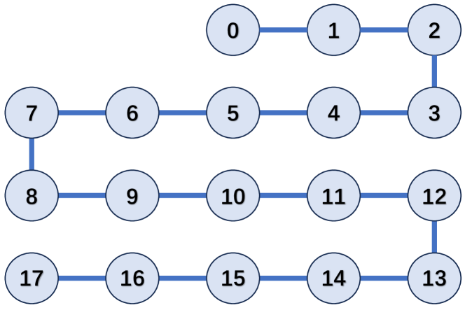
Figure 14: Diagram of ScQ-P18 processor of the on-cloud Quafu quantum computers.

Qubit index	2	3	4	5
Qubit frequency, $f_{10}$ ($\mathrm{GHz}$)	4.620	5.071	4.500	4.982
Readout frequency, $f_{r}$ ($\mathrm{GHz}$)	6.737	6.713	6.693	6.675
Anharmonicity, $\eta$ ($\mathrm{MHz}$)	-202.6	-198.0	-204.8	-193.7
Relaxation time, $T_{1}$ ($\mu\mathrm{s}$)	41.4	40.1	29.0	23.6
Coherence time, $T_{2}$ ($\mu\mathrm{s}$)	4.8	2.3	5.7	2.2

Table 2: The parameters of the four used qubits.

E.1 The Theoretical Calculation

E.1.1 ICO scheme

When $D_{\textrm{tb}}=D_{\textrm{t}}=2$, we cannot use the asymptotic result of output in equation (24) For this case, the non-diagonal state is

$$\tilde{\rho}_{\textrm{t}}= \ \left(p+\frac{1}{D_{\textrm{t}}^{2}-1}\right)\rho_{\textrm{t}}+\frac{1}{D_{\textrm{t}}^{2}-1}\sum_{k}\hat{M}_{k}^{\dagger}\rho_{\textrm{t}}\hat{M}_{k}-\frac{1}{D_{\textrm{t}}(D_{\textrm{t}}^{2}-1)}\sum_{k}[\mathrm{Tr}(\hat{M}_{k})\rho_{\textrm{t}}\hat{M}_{k}^{\dagger}+\mathrm{Tr}(\hat{M}_{k}^{\dagger})\hat{M}_{k}\rho_{\textrm{t}}]$$ (81)

$$= \ \frac{1}{3}\rho_{\textrm{t}}+\frac{1}{3}\sum_{k}\hat{M}_{k}^{\dagger}\rho_{\textrm{t}}\hat{M}_{k}=\frac{1}{2}\rho_{\textrm{t}}+\frac{1}{6}\hat{\sigma}_{\textrm{t}}^{\bm{r}}\rho_{\textrm{t}}\hat{\sigma}_{\textrm{t}}^{\bm{r}},$$ (82)

and $\langle\hat{\sigma}_{\textrm{c}}^{x}\rangle=\mathrm{Tr}\tilde{\rho}_{\textrm{t}}=\frac{2}{3}$. Thus, we get the output state recovering information as

$$\rho_{\textrm{t}}^{+}=\frac{1}{2}\rho_{\textrm{t}}+\frac{1}{10}\hat{\sigma}_{\textrm{t}}^{\bm{r}}\rho_{\textrm{t}}\hat{\sigma}_{\textrm{t}}^{\bm{r}}+\frac{2}{5}\frac{\hat{\mathbb{I}}}{D_{\textrm{t}}},$$ (83)

and the fidelity $F={(7+r_{z}^{2})}/{10}$, where $r_{z}=\cos\theta$ is the component of vector ${\bm{r}}$ in $z$ direction.

E.1.2 MDD scheme

In this situation, the assumption the dimension $D_{\textrm{tb}}\rightarrow\infty$ goes to infinity fails when we use the Clifford group to mimic the Haar measure of a single qubit. Without the asymptotic assumption, the result of output state is

$$\rho_{\textrm{atb}}=\frac{1}{2}\hat{\mathbb{I}}_{\textrm{a}}\otimes[p\rho_{\textrm{tb}}+(1-p)\hat{\mathbb{I}}/D_{\textrm{tb}}]+\frac{1}{2}\hat{\sigma}_{\textrm{a}}^{x}\otimes[p^{\prime}\rho_{\textrm{tb}}+(r_{x}^{2}-p^{\prime})\hat{\mathbb{I}}/D_{\textrm{tb}}],$$

where $p={1}/{3},p^{\prime}={(2-r_{x}^{2})}/{3}$ by $D_{\textrm{tb}}=D_{\textrm{t}}=2$. For we only concern about the fidelity of state with $\ket{+}$ in control qubit $q_{\textrm{a}}$, the corresponding state is

$$\rho_{\textrm{t}}^{+}=\frac{3-r_{x}^{2}}{3(1+r_{x}^{2})}\rho_{\textrm{t}}+\frac{2r_{x}^{2}}{3(1+r_{x}^{2})}{\hat{\mathbb{I}}_{\textrm{t}}},$$ (84)

and the fidelity with initial state $\ket{0}$ is $F={2}/{3(1+r_{x}^{2})}+{1}/{3}$.

E.1.3 Combination of ICO and MDD schemes

For the diagonal part of $q_{\textrm{a}}$, the states of $q_{\textrm{c}},q_{\textrm{t}}$ is same as the case only with the ICO scheme, thus $\langle\hat{\sigma}_{\textrm{c}}^{x}\rangle=\mathrm{Tr}\tilde{\rho}_{\textrm{t}}={2}/{3}$, and the state of $q_{\textrm{t}}$ after post-selection on $q_{\textrm{c}}$ without normalization is

$$\rho_{\textrm{t}1}^{+}=\frac{5}{12}\rho_{\textrm{t}}+\frac{1}{12}\hat{\sigma}_{\textrm{t}}^{\bm{r}}\rho_{\textrm{t}}\hat{\sigma}_{\textrm{t}}^{\bm{r}}+\frac{\hat{\mathbb{I}}_{\textrm{t}}}{6}.$$

For the non-diagonal part of $q_{\textrm{a}}$, the reduced state of $q_{\textrm{c}},q_{\textrm{t}}$ is

$$\rho_{\textrm{ct}2}= \frac{1}{2}\hat{\mathbb{I}}_{\textrm{c}}\otimes[p^{\prime}\rho_{\textrm{t}}+(r_{x}^{2}-p^{\prime})\hat{\mathbb{I}}/d]$$

$$+\frac{1}{2}\hat{\sigma}^{x}\otimes[(p+{1}/{6})\rho_{\textrm{t}}+\hat{\sigma}_{\textrm{t}}^{\bm{r}}\rho\hat{\sigma}_{\textrm{t}}^{{\bm{r}}^{\prime}}/6],$$ (85)

thus $\langle\hat{\sigma}_{\textrm{a}}^{x}\rangle=\mathrm{Tr}(\rho_{\textrm{ct}2})=r_{x}^{2}$, and the state of $q_{\textrm{t}}$ without normalization is

$$\rho_{\textrm{t}2}^{+}=\left(\frac{7}{12}-\frac{r_{x}^{2}}{6}\right)\rho_{\textrm{t}}+\frac{1}{12}\hat{\sigma}_{\textrm{t}}^{\bm{r}}\rho_{\textrm{t}}\hat{\sigma}_{\textrm{t}}^{{\bm{r}}^{\prime}}+\frac{2r_{x}^{2}-1}{6}{\hat{\mathbb{I}}_{\textrm{t}}}.$$

Here we select ${\bm{r}}=(r_{x},0,r_{z})$ in circuit, thus ${\bm{r}}^{\prime}=(r_{x},0,-r_{z})$. Then we get the normalized state of interest

$$\rho_{\textrm{t}}^{++}=\frac{1}{3+2r_{x}^{2}}\left[\left(3-\frac{r_{x}^{2}}{2}\right)\rho_{\textrm{t}}+\frac{\hat{\sigma}_{\textrm{t}}^{\bm{r}}\rho_{\textrm{t}}\hat{\sigma}^{{\bm{r}}^{\prime}}+\hat{\sigma}_{\textrm{t}}^{\bm{r}}\rho_{\textrm{t}}\hat{\sigma}_{\textrm{t}}^{\bm{r}}}{4}+r_{x}^{2}{\hat{\mathbb{I}}_{\textrm{t}}}\right]$$ (86)

with successful probability $p_{++}=({2r_{x}^{2}+3})/{6}$, and the fidelity $F={9}/({8r_{x}^{2}+12})+{1}/{4}$.

E.2 Error mitigation

To mitigate the error in experiment, we treat the twirling channel as a whole. Notice that when perturbation channel $\Lambda=\Lambda^{0}\equiv\mathcal{I}$, theoretically the twirling channel of it is also $\Lambda_{\mathrm{twirl}}=\Lambda_{\mathrm{twirl}}^{0}\equiv\mathcal{I}$, thus in practical the twirling channel with error is just the error channel $\Lambda_{\mathrm{twirl}}^{0}=\mathcal{E}$. For general perturbation channel $\Lambda$, the twirling channel with error is $\Lambda_{\mathrm{twirl}}^{e}=\mathcal{E}\circ\Lambda_{\mathrm{twirl}}$. So we have to gain adequate knowledge about the error channel $\mathcal{E}$ to deal with the error. However, to perform QPT on an operation of $d$ dimension space, there are $d^{4}-d^{2}$ parameters needed to be determined. Thus, we want to reduce the parameters needed to process the error.

In our circuit, the output state of auxiliary or control qubit $q_{\textrm{c}}$ and the target qubit $q_{\textrm{t}}$ after twirling channel $\Lambda_{\mathrm{twirl}}$ can be written as

$$\rho_{\textrm{ct}}=\Lambda_{\mathrm{twirl}}(\rho_{\textrm{ct}})=(\hat{\mathbb{I}}_{\textrm{c}}\otimes\rho_{\textrm{t}0}+\hat{\sigma}_{\textrm{c}}^{x}\otimes\rho_{\textrm{t}1})/2=[\ket{+}_{\textrm{c}}\bra{+}\otimes(\rho_{\textrm{t}0}+\rho_{\textrm{t}1})+\ket{-}_{\textrm{c}}\bra{-}\otimes(\rho_{\textrm{t}0}-\rho_{\textrm{t}1})]/2,$$ (87)

where $\rho_{\textrm{t}0},\rho_{\textrm{t}1}$ is normalized state of $q_{\textrm{t}}$. Thus, what we need to know is the action of error channel $\mathcal{E}$ on state $\ket{\pm}_{\textrm{c}}\bra{\pm}\otimes\rho_{\textrm{t}}$. The joint state space of two qubits $q_{\textrm{c}}$, $q_{\textrm{t}}$ is the tensor product space of state space of $q_{\textrm{c}}$ and $q_{\textrm{t}}$, and the bases of tensor space are the tensor products of the bases of $q_{\textrm{c}}$ and $q_{\textrm{t}}$. Selecting the Pauli matrix $\sigma^{\mu},(\mu=0,1,2,3)$, as the bases of state space of qubits $q_{\textrm{c}}$ and $q_{\textrm{t}}$, the bases of the tensor space is $\hat{\sigma}_{\textrm{c}}^{\mu}\otimes\hat{\sigma}_{\textrm{t}}^{\nu}$, and the joint state of $q_{\textrm{c}},q_{\textrm{t}}$ can be decomposed as

$$\mathcal{E}(\ket{\pm}_{\textrm{c}}\bra{\pm}\otimes\rho_{\textrm{t}})=\frac{1}{2}\sum_{\mu,\nu}\chi_{\mu\nu}^{\pm}\hat{\sigma}_{\textrm{c}}^{\mu}\otimes\hat{\sigma}_{\textrm{t}}^{\nu}=\frac{1}{2}\sum_{\mu}p_{\mu}^{\pm}\hat{\sigma}_{\textrm{c}}^{\mu}\otimes\rho_{\textrm{t}}^{\mu\pm},$$

where $p_{\mu}^{\pm}\rho_{\mu}^{\pm}=\sum_{\nu}\chi_{\mu\nu}^{\pm}\hat{\sigma}_{\nu}$, $\rho_{\mu}$ is normalized, and $p_{0}^{\pm}=1$ to make sure $\mathcal{E}$ preserving the trace of state. Then we denote the completely positive trace preserving (CPTP) operator mapping $\rho$ to $\rho_{\mu}^{\pm}$ as $\mathcal{E}_{\mu}^{\pm}$, we have

$$\mathcal{E}(\ket{\pm}_{\textrm{c}}\bra{\pm}\otimes\rho_{\textrm{t}})=\frac{1}{2}\sum_{\mu}p_{\mu}^{\pm}\hat{\sigma}_{\textrm{c}}^{\mu}\otimes\mathcal{E}_{\mu}^{\pm}(\rho_{\textrm{t}}).$$ (88)

Applying this result to the twirling channel with error, we have

$$\rho^{e}_{\textrm{ct}}=\Lambda_{\mathrm{twirl}}^{e}(\rho_{\textrm{c}})=\frac{1}{4}\sum_{\mu}\hat{\sigma}_{\textrm{c}}^{\mu}\otimes\left[p_{\mu}^{+}\mathcal{E}_{\mu}^{+}(\rho_{\textrm{t}}^{+})+p_{\mu}^{-}\mathcal{E}_{\mu}^{-}(\rho_{\textrm{t}}^{-})\right],$$ (89)

where $\rho_{\textrm{t}}^{\pm}=\rho_{\textrm{t}0}\pm\rho_{\textrm{t}1}$.

When measure $\hat{\sigma}_{\textrm{c}}^{x}$ on $q_{\textrm{c}}$, we consider the reduced density matrix of $q_{\textrm{c}}$,

$$\rho_{\textrm{c}} =\hat{\mathbb{I}}_{\textrm{c}}/2+q\hat{\sigma}_{\textrm{c}}^{x}/2,$$ (90)

$$\rho_{\textrm{c}}^{e} =\hat{\mathbb{I}}_{\textrm{c}}/2+\sum_{i}\hat{\sigma}_{\textrm{c}}^{i}[p_{i}^{+}(1+q)+p_{i}^{-}(1-q)]/4,$$ (91)

where $q=\mathrm{Tr}\rho_{\textrm{t}1}$, and $i=1,2,3$. For the twirling channel with or without error, we have

$$\braket{\hat{\sigma}_{\textrm{c}}^{x}}=q,\qquad\braket{\hat{\sigma}_{\textrm{c}}^{x}}_{e}=\frac{1}{2}[p_{1}^{+}(1+q)+p_{1}^{-}(1-q)],$$

and for the error channel with initial state $\ket{\pm}_{\textrm{c}}\otimes\rho_{\textrm{t}}$,

$$\braket{\hat{\sigma}_{\textrm{c}}^{x}}_{\pm}=p_{1}^{\pm}.$$

So the expectation $\braket{\hat{\sigma}_{\textrm{c}}^{x}}_{e}$ of twirling channel with error can be evaluated by the expectation without error $\braket{\hat{\sigma}_{\textrm{c}}{x}}$ and of the error channel $\braket{\hat{\sigma}_{\textrm{c}}^{x}}_{\pm}$,

$$\braket{\hat{\sigma}_{\textrm{c}}^{x}}_{e}=\frac{\braket{\hat{\sigma}_{\textrm{c}}^{x}}_{+}+\braket{\hat{\sigma}_{\textrm{c}}^{x}}_{-}}{2}+\frac{\braket{\hat{\sigma}_{\textrm{c}}^{x}}_{+}-\braket{\hat{\sigma}_{\textrm{c}}^{x}}_{-}}{2}\braket{\hat{\sigma}_{\textrm{c}}^{x}},$$ (92)

where $\braket{\hat{\sigma}_{\textrm{c}}^{x}}$ is the theoretical value, and the $\braket{\hat{\sigma}_{\textrm{c}}^{x}}_{\pm}$ can be measured from the experiment by removing perturbation and setting corresponding initial state on $q_{\textrm{c}}$.

When calculation the fidelity of $q_{\textrm{t}}$, we should consider the reduced matrix of $q_{\textrm{t}}$, and particularly, we post select the state of $q_{\textrm{t}}$ with $q_{\textrm{c}}$ in $\ket{+}_{\textrm{c}}$ state. The reduced matrix of $q_{\textrm{t}}$

$$\rho_{\textrm{t}}^{e+}=\ \frac{[(1+p_{1}^{+})\mathcal{E}^{+}+(1+p_{1}^{-})\mathcal{E}^{-}](\rho_{\textrm{t}0})}{2+(p_{1}^{+}+p_{1}^{-})+q(p_{1}^{+}-p_{1}^{-})}+\frac{[(1+p_{1}^{+})\mathcal{E}^{+}-(1+p_{1}^{-})\mathcal{E}^{-}](\rho_{\textrm{t}1})}{2+(p_{1}^{+}+p_{1}^{-})+q(p_{1}^{+}-p_{1}^{-})}$$ (93)

where $\mathcal{E}^{\pm}=\left(\mathcal{E}_{0}^{\pm}+p_{1}^{\pm}\mathcal{E}_{1}^{\pm}\right)/(1+p_{1}^{\pm})$ is the normalized error channel on $q_{\textrm{t}}$ with initial state $\ket{\pm}_{\textrm{c}}$ and post selected by $\ket{+}_{\textrm{c}}$ on $q_{\textrm{c}}$. To calculate the fidelity explicitly, we need to consider the circuit in detail.

E.2.1 ICO scheme

In this scheme, as we have shown previously,

$$\rho_{\textrm{t}1}=\frac{1}{3}\rho_{\textrm{t}}+\frac{1}{3}\hat{\mathbb{I}}_{\textrm{t}},\qquad\rho_{\textrm{t}2}=\frac{1}{2}\rho_{\textrm{t}}+\frac{1}{6}\hat{\sigma}_{\textrm{t}}^{\bm{r}}\rho_{\textrm{t}}\hat{\sigma}_{\textrm{t}}^{\bm{r}},$$

and $q={2}/{3}$. So the problem reduce to calculate the fidelities between $\mathcal{E}^{\pm}(\rho_{\textrm{t}})$ or $\mathcal{E}^{\pm}(\hat{\sigma}_{\textrm{t}}^{\bm{r}}\rho_{\textrm{t}}\hat{\sigma}_{\textrm{t}}^{\bm{r}})$ and $\rho_{\textrm{t}}$, where $\rho_{\textrm{t}}$ is a pure state.

For $\mathcal{E}^{\pm}(\rho_{\textrm{t}})$, the fidelity $F^{\pm}=\mathrm{Tr}[\rho_{\textrm{t}}\mathcal{E}^{\pm}(\rho_{\textrm{t}})]$ can be set as the average fidelity of channel $\mathcal{E}^{\pm}$, which can be measured by removing the perturbation in our circuit. For $\mathcal{E}^{\pm}(\hat{\sigma}_{\textrm{t}}^{\bm{r}}\rho_{\textrm{t}}\hat{\sigma}_{\textrm{t}}^{\bm{r}})$ with $\hat{\sigma}_{\textrm{t}}^{\bm{r}}\equiv{\bm{r}}\cdot\hat{\sigma}_{\textrm{t}}$ and $\rho_{\textrm{t}}=|0\rangle_{\textrm{t}}\langle 0|$, the fidelity

$$\mathrm{Tr}[\rho_{\textrm{t}}\mathcal{E}^{\pm}(\hat{\sigma}_{\textrm{t}}^{\bm{r}}\rho_{\textrm{t}}\hat{\sigma}_{\textrm{t}}^{\bm{r}})]= \ \braket{0}{\mathcal{E}^{\pm}(\hat{\sigma}_{\textrm{t}}^{\bm{r}}}{0\rangle_{\textrm{t}}\langle 0|\hat{\sigma}_{\textrm{t}}^{\bm{r}})|0}$$

$$= \sum_{i,j=0,1}\bra{i|\hat{\sigma}_{\textrm{t}}^{\bm{r}}|0}\braket{0}{\hat{\sigma}_{\textrm{t}}^{\bm{r}}}{j}\braket{0}{\mathcal{E}^{\pm}(}{i\rangle_{\textrm{t}}\langle j|)|0}$$ (94)

$$= \ \left|\braket{0}{\hat{\sigma}_{\textrm{t}}^{\bm{r}}}{0}\right|^{2}\braket{0}{\mathcal{E}^{\pm}(}{0\rangle_{\textrm{t}}\langle 0|)|0}+\left|\braket{1}{\hat{\sigma}_{\textrm{t}}^{\bm{r}}}{0}\right|^{2}\braket{0}{\mathcal{E}^{\pm}(}{1\rangle_{\textrm{t}}\langle 1|)|0}$$

$$+\braket{0}{\hat{\sigma}_{\textrm{t}}^{\bm{r}}}{0}\braket{0}{\hat{\sigma}_{\textrm{t}}^{\bm{r}}}{1}\braket{0}{\mathcal{E}^{\pm}(}{0\rangle_{\textrm{t}}\langle 1|)|0}+\braket{1}{\hat{\sigma}_{\textrm{t}}^{\bm{r}}}{0}\braket{0}{\hat{\sigma}_{\textrm{t}}^{\bm{r}}}{0}\braket{0}{\mathcal{E}^{\pm}(}{1\rangle_{\textrm{t}}\langle 0|)|0}.$$ (95)

With ${\bm{r}}=(r_{x},0,r_{z})$, we have $\braket{0}{\hat{\sigma}_{\textrm{t}}^{\bm{r}}}{0}=r_{z},\braket{0}{\hat{\sigma}_{\textrm{t}}^{\bm{r}}}{1}=\braket{1}{\hat{\sigma}_{\textrm{t}}^{\bm{r}}}{0}=r_{x}$. As before, we can set $\braket{0}{\mathcal{E}^{\pm}(}{0\rangle_{\textrm{t}}\langle 0|)|0}=F^{\pm}$, then $\braket{0}{\mathcal{E}^{\pm}(}{1\rangle_{\textrm{t}}\langle 1|)|0}=1-F^{\pm}$ can be verified. We can also assume that the error channel $\mathcal{E}^{\pm}$ is Hermitian, for the circuit of $\Lambda_{t}^{0}=\mathcal{E}^{\pm}$ is invariant under time reversing. With above results, we can represent the fidelity as

$$\mathrm{Tr}[\rho_{\textrm{t}}\mathcal{E}^{\pm}(\hat{\sigma}_{\textrm{t}}^{\bm{r}}\rho_{\textrm{t}}\hat{\sigma}^{\bm{r}})]=r_{z}^{2}F^{\pm}+r_{x}^{2}(1-F^{\pm})+r_{x}r_{z}\mathrm{Tr}[\hat{\sigma}_{\textrm{t}}^{x}\mathcal{E}^{\pm}(|0\rangle_{\textrm{t}}\langle 0|)],$$

and the problem is to calculate the polarization of state after error channel.

In general, the state after error channel is not a pure state and is expressed as

$$\mathcal{E}^{\pm}(|0\rangle_{\textrm{t}}\langle 0|)=F^{\pm}|0\rangle_{\textrm{t}}\langle 0|+(1-F^{\pm})|0\rangle_{\textrm{t}}\langle 0|+r(e^{\imath\theta}|0\rangle_{\textrm{t}}\langle 1|+e^{-\imath\theta}|1\rangle_{\textrm{t}}\langle 0|).$$ (96)

Then, we have $\mathrm{Tr}[\hat{\sigma}_{x}\mathcal{E}^{\pm}(|0\rangle_{\textrm{t}}\langle 0|)]=2r\cos\theta$. Because our circuit is average over Clifford group, in this average,

$$\langle\cos\theta\rangle=\frac{1}{N}\sum_{\phi_{i}}\cos(\phi_{i}+\theta)\approx\int\!\!d\phi\;\cos(\phi+\theta)=0,$$

the polarization $\mathrm{Tr}[\hat{\sigma}_{x}\mathcal{E}^{\pm}(|0\rangle_{\textrm{t}}\langle 0|)]=0$, and

$$\mathrm{Tr}[\rho\mathcal{E}^{\pm}(\hat{\sigma}_{\textrm{t}}^{\bm{r}}\rho_{\textrm{t}}\hat{\sigma}_{\textrm{t}}^{\bm{r}})]=r_{z}^{2}F^{\pm}+r_{x}^{2}(1-F^{\pm}).$$

Then the fidelities of $\rho_{\textrm{t}0},\rho_{\textrm{t}1}$ with respect to $\rho_{\textrm{t}}$ are

$$\begin{split}F_{0}^{\pm}&=\frac{1}{3}F^{\pm}+\frac{1}{3},\\ F_{1}^{\pm}&=\frac{2-r_{x}^{2}}{3}F^{\pm}+\frac{1}{6}r_{x}^{2}.\end{split}$$

The fidelity of twirling channel with error and the expectation $\braket{\hat{\sigma}_{\textrm{c}}^{x}}_{e}$ are

$$F^{e}= \ \frac{(1+\braket{\hat{\sigma}_{\textrm{c}}^{x}}_{+})(1+F^{+})+(1+\braket{\hat{\sigma}_{\textrm{c}}^{x}}_{-})(1+F^{-})}{6+3(\braket{\hat{\sigma}_{\textrm{c}}^{x}}_{+}+\braket{\hat{\sigma}_{\textrm{c}}^{x}}_{-})+2(\braket{\hat{\sigma}_{\textrm{c}}^{x}}_{+}-\braket{\hat{\sigma}_{\textrm{c}}^{x}}_{-})}+\frac{(2-r_{x}^{2})[(1+\braket{\hat{\sigma}_{\textrm{c}}^{x}}_{+})F^{+}-(1+\braket{\hat{\sigma}_{\textrm{c}}^{x}}_{-})F^{-}]}{6+3(\braket{\hat{\sigma}_{\textrm{c}}^{x}}_{+}+\braket{\hat{\sigma}_{\textrm{c}}^{x}}_{-})+2(\braket{\hat{\sigma}_{\textrm{c}}^{x}}_{+}-\braket{\hat{\sigma}_{\textrm{c}}^{x}}_{-})}$$

$$\ +\frac{r_{x}^{2}}{2}\frac{\braket{\hat{\sigma}_{\textrm{c}}^{x}}_{+}-\braket{\hat{\sigma}_{\textrm{c}}^{x}}_{-}}{6+3(\braket{\hat{\sigma}_{\textrm{c}}^{x}}_{+}+\braket{\hat{\sigma}_{\textrm{c}}^{x}}_{-})+2(\braket{\hat{\sigma}_{\textrm{c}}^{x}}_{+}-\braket{\hat{\sigma}_{\textrm{c}}^{x}}_{-})},$$ (97)

$$\braket{\hat{\sigma}_{\textrm{c}}^{x}}_{e}= \ \frac{\braket{\hat{\sigma}_{\textrm{c}}^{x}}_{+}+\braket{\hat{\sigma}_{\textrm{c}}^{x}}_{-}}{2}+\frac{\braket{\hat{\sigma}_{\textrm{c}}^{x}}_{+}-\braket{\hat{\sigma}_{\textrm{c}}^{x}}_{-}}{3},$$ (98)

where $\braket{\hat{\sigma}_{\textrm{c}}^{x}}_{\pm},F^{\pm}$ are measured from circuit of the twirling channel $\Lambda_{\mathrm{twirl}}^{0}$ of identical channel $\mathcal{I}$ with corresponding initial states $\ket{\pm}_{\textrm{c}}$ of $q_{\textrm{c}}$ and post-selected on the state $\ket{+}_{\textrm{c}}$.

E.2.2 MDD scheme

In this scheme, as shown in previous,

$$\rho_{\textrm{t}0}=\frac{1}{3}\rho_{\textrm{t}}+\frac{2}{6}\hat{\mathbb{I}}_{\textrm{t}},\qquad\rho_{\textrm{t}1}=\frac{2-r_{x}^{2}}{3}\rho_{\textrm{t}}+\frac{2r_{x}^{2}-1}{3}\hat{\mathbb{I}}_{\textrm{t}},$$ (99)

and $q=r_{x}^{2}$. It is also obvious from previous,

$$\begin{split}F_{0}^{\pm}&=\frac{1}{3}F^{\pm}+\frac{1}{3},\\ F_{1}^{\pm}&=\frac{2-r_{x}^{2}}{3}F^{\pm}+\frac{2r_{x}^{2}-1}{3},\end{split}$$

thus the fidelity of twirling channel with error

$$F^{e}= \ \frac{1}{3}\frac{(1+\braket{\hat{\sigma}_{\textrm{a}}^{x}}_{+})(1+F^{+})+(1+\braket{\hat{\sigma}_{\textrm{a}}^{x}}_{-})(1+F^{-})}{2+\braket{\hat{\sigma}_{\textrm{a}}^{x}}_{+}+\braket{\hat{\sigma}_{\textrm{a}}^{x}}_{-}+r_{x}^{2}(\braket{\hat{\sigma}_{\textrm{a}}^{x}}_{+}-\braket{\hat{\sigma}_{\textrm{a}}^{x}}_{-})}+\frac{(2-r_{x}^{2})}{3}\frac{(1+\braket{\hat{\sigma}_{\textrm{a}}^{x}}_{+})F^{+}-(1+\braket{\hat{\sigma}_{\textrm{a}}^{x}}_{-})F^{-}}{2+\braket{\hat{\sigma}_{\textrm{a}}^{x}}_{+}+\braket{\hat{\sigma}_{\textrm{a}}^{x}}_{-}+r_{x}^{2}(\braket{\hat{\sigma}_{\textrm{a}}^{x}}_{+}-\braket{\hat{\sigma}_{\textrm{a}}^{x}}_{-})}$$

$$\ +\frac{2r_{x}^{2}-1}{3}\frac{\braket{\hat{\sigma}_{\textrm{a}}^{x}}_{+}-\braket{\hat{\sigma}_{\textrm{a}}^{x}}_{-}}{2+\braket{\hat{\sigma}_{\textrm{a}}^{x}}_{+}+\braket{\hat{\sigma}_{\textrm{a}}^{x}}_{-}+r_{x}^{2}(\braket{\hat{\sigma}_{\textrm{a}}^{x}}_{+}-\braket{\hat{\sigma}_{\textrm{a}}^{x}}_{-})},$$ (100)

$$\braket{\hat{\sigma}_{\textrm{a}}^{x}}_{e}= \ \frac{\braket{\hat{\sigma}_{\textrm{a}}^{x}}_{+}+\braket{\hat{\sigma}_{\textrm{a}}^{x}}_{-}}{2}+r_{x}^{2}\frac{\braket{\hat{\sigma}_{\textrm{a}}^{x}}_{+}-\braket{\hat{\sigma}_{\textrm{a}}^{x}}_{-}}{2},$$ (101)

The quantities $\braket{\hat{\sigma}_{\textrm{a}}^{x}}_{\pm},F^{\pm}$ is measured as before.

E.2.3 Combination of ICO and MDD scheme

In this scheme, there are two error channel, where $\mathcal{E}_{\textrm{a}}$ is the channel applied on qubits $q_{\textrm{t}}$, $q_{\textrm{a}}$, which same as the one in MDD scheme, and $\mathcal{E}_{\textrm{c}}$, is applied on qubit $q_{\textrm{c}}$, $q_{\textrm{t}}$, which is same as the recovery in ICO scheme. Thus, the expectation of $\hat{\sigma}^{x}$ on control qubit $q_{\textrm{c}}$ and auxiliary qubit $q_{\textrm{a}}$ are same as previous two schemes,

$$\begin{split}\braket{\hat{\sigma}_{\textrm{c}}^{x}}_{e}=&\ \frac{\braket{\hat{\sigma}_{\textrm{c}}^{x}}_{+}+\braket{\hat{\sigma}_{\textrm{c}}^{x}}_{-}}{2}+r_{x}^{2}\frac{\braket{\hat{\sigma}_{\textrm{c}}^{x}}_{+}-\braket{\hat{\sigma}_{\textrm{c}}^{x}}_{-}}{2},\\ \braket{\hat{\sigma}_{\textrm{a}}^{x}}_{e}=&\ \frac{\braket{\hat{\sigma}_{\textrm{a}}^{x}}_{+}+\braket{\hat{\sigma}_{\textrm{a}}^{x}}_{-}}{2}+\frac{\braket{\hat{\sigma}_{\textrm{a}}^{x}}_{+}-\braket{\hat{\sigma}_{\textrm{a}}^{x}}_{-}}{3}.\end{split}$$ (102)

The diagonal part of the auxiliary qubit $q_{\textrm{a}}$ is same as the scheme of recovery in ICO, thus the reduced density matrix of $q_{\textrm{t}}$ of $\rho_{\textrm{t}0}$ without normalization is

$${\rho}_{\textrm{t}0}= \ \frac{1}{24}(1+p_{1\textrm{c}}^{+})[5\mathcal{E}_{\textrm{c}}^{+}(\rho_{\textrm{t}})+\mathcal{E}_{\textrm{c}}^{+}(\hat{\sigma}_{\textrm{t}}^{\bm{r}}\rho_{\textrm{t}}\hat{\sigma}_{\textrm{t}}^{\bm{r}})]-\frac{1}{24}(1+p_{1\textrm{c}}^{-})[\mathcal{E}_{\textrm{c}}^{-}(\rho_{\textrm{t}})+\mathcal{E}_{\textrm{c}}^{-}(\hat{\sigma}_{\textrm{t}}^{\bm{r}}\rho_{\textrm{t}}\hat{\sigma}_{\textrm{t}}^{\bm{r}})]+\frac{1}{12}(2+p_{1\textrm{c}}^{+}+p_{1\textrm{c}}^{-}){\hat{\mathbb{I}}_{\textrm{t}}}$$ (103)

The coherent part is shown in previous as

$$\rho_{\textrm{ct}1}=\frac{1}{2}\left(\hat{\mathbb{I}}_{\textrm{c}}\otimes\left[\frac{2-r_{x}^{2}}{3}\rho_{\textrm{t}}+\frac{2(2r_{x}^{2}-1)}{6}\hat{\mathbb{I}}_{\textrm{t}}\right]+\hat{\sigma}_{\textrm{c}}^{x}\otimes\left[\frac{1}{2}\rho_{\textrm{t}}+\frac{1}{6}\hat{\sigma}_{\textrm{t}}^{\bm{r}}\rho_{\textrm{t}}\hat{\sigma}_{\textrm{t}}^{{\bm{r}}^{\prime}}\right]\right),$$ (104)

Then we consider the reduced density matrix of $q_{\textrm{t}}$ after error channel $\mathcal{E}_{c}$, the reduced density matrix of $q_{\textrm{t}}$ without normalization is

$${\rho}_{\textrm{t}1}= \ \frac{1}{24}(1+p_{1\textrm{c}}^{+})[(7-2r_{x}^{2})\mathcal{E}_{\textrm{c}}^{+}(\rho_{\textrm{t}})+\mathcal{E}_{\textrm{c}}^{+}(\hat{\sigma}_{\textrm{t}}^{\bm{r}}\rho_{\textrm{t}}\hat{\sigma}_{\textrm{t}}^{{\bm{r}}^{\prime}})]+\frac{1}{24}(1+p_{1\textrm{c}}^{-})[(1-2r_{x}^{2})\mathcal{E}_{\textrm{c}}^{-}(\rho_{\textrm{t}})-\mathcal{E}_{\textrm{c}}^{-}(\hat{\sigma}_{\textrm{t}}^{\bm{r}}\rho_{\textrm{t}}\hat{\sigma}_{\textrm{t}}^{{\bm{r}}^{\prime}})]$$

$$+\frac{2r_{x}^{2}-1}{12}(2+p_{1\textrm{c}}^{+}+p_{1\textrm{c}}^{-}){\hat{\mathbb{I}}_{\textrm{t}}}.$$ (105)

Then the reduced state of $q_{\textrm{t}}$, $q_{\textrm{a}}$ by post selection on $q_{\textrm{c}}$ without normalization is

$$\rho_{\textrm{ta}}=\frac{1}{2}({\rho}_{\textrm{t}0}\otimes\hat{\mathbb{I}}_{\textrm{a}}+{\rho}_{\textrm{t}1}\otimes\hat{\sigma}_{\textrm{a}}^{x}),$$

and after performing the error channel $\mathcal{E}_{\textrm{a}}$ and post-selecting $q_{\textrm{a}}$, the normalized state can be written as

$$\rho_{\textrm{t}}^{++}=\frac{1}{4p_{++}}\left[\left((1+p_{1\textrm{a}}^{+})\mathcal{E}_{\textrm{a}}^{+}+(1+p_{1\textrm{a}}^{-})\mathcal{E}_{\textrm{a}}^{-}\right)({\rho}_{\textrm{t}0})+\left((1+p_{1\textrm{a}}^{+})\mathcal{E}_{\textrm{a}}^{+}-(1+p_{1\textrm{a}}^{-})\mathcal{E}_{\textrm{a}}^{-}\right)({\rho}_{\textrm{t}1})\right]$$

with the probability

$$p_{++} =\ \mathrm{Tr}\rho_{\textrm{t}}^{++}$$

$$=\ \frac{2+p_{1\textrm{a}}^{+}+p_{1\textrm{a}}^{-}}{16}\left[2+p_{1\textrm{c}}^{+}+p_{1\textrm{c}}^{-}+\frac{2}{3}(p_{1\textrm{c}}^{+}-p_{1\textrm{c}}^{-})\right]+\frac{p_{1\textrm{a}}^{+}-p_{1\textrm{a}}^{-}}{16}\left[(2+p_{1\textrm{c}}^{+}+p_{1\textrm{c}}^{-})r_{x}^{2}+\frac{1}{3}(r_{x}^{2}+1)(p_{1\textrm{c}}^{+}-p_{1\textrm{c}}^{-})\right].$$

The fidelity of this state with the initial state reduces to the fidelity of $\mathcal{E}_{\textrm{a}}^{\pm}\circ\mathcal{E}_{\textrm{c}}^{\pm}(\rho),\mathcal{E}_{\textrm{a}}^{\pm}\circ\mathcal{E}_{\textrm{c}}^{\pm}(\hat{\sigma}^{\bm{r}}\rho\hat{\sigma}^{\bm{r}})$, and $\mathcal{E}_{\textrm{a}}^{\pm}\circ\mathcal{E}_{\textrm{c}}^{\pm}(\hat{\sigma}^{\bm{r}}\rho\hat{\sigma}^{{\bm{r}}^{\prime}})$.

Denoting $F^{\pm\pm}\equiv\mathrm{Tr}\left[\rho_{\textrm{t}}\mathcal{E}^{\pm\pm}(\rho_{\textrm{t}})\right]$, where $\mathcal{E}^{\pm\pm}\equiv\mathcal{E}_{\textrm{a}}^{\pm}\circ\mathcal{E}_{\textrm{c}}^{\pm}$, it can be measured from the fidelity of error channel on $q_{\textrm{t}}$ with an initial state $\ket{\pm}_{\textrm{c}}\otimes\ket{\pm}_{\textrm{a}}$ of $q_{\textrm{c}},q_{\textrm{a}}$. Similarly, we have

$$\mathrm{Tr}[\rho_{\textrm{t}}\mathcal{E}^{\pm\pm}(\hat{\sigma}^{\bm{r}}\rho_{\textrm{t}}\hat{\sigma}^{\bm{r}})]=r_{z}^{2}F^{\pm\pm}+r_{x}^{2}(1-F^{\pm\pm}),$$

and

$$\mathrm{Tr}[\rho_{\textrm{t}}\mathcal{E}^{\pm\pm}(\hat{\sigma}_{\textrm{t}}^{\bm{r}}\rho_{\textrm{t}}\hat{\sigma}_{\textrm{t}}^{\bm{r}^{\prime}})]= \ \braket{0}{\mathcal{E}^{\pm\pm}([\hat{\sigma}_{\textrm{t}}^{\bm{r}}}{0\rangle_{\textrm{t}}\langle 0|\hat{\sigma}_{\textrm{t}}^{\bm{r}^{\prime}}])|0}$$ (106)

$$= \sum_{i,j=0,1}\braket{i}{\hat{\sigma}_{\textrm{t}}^{\bm{r}}}{0}\braket{0}{\hat{\sigma}_{\textrm{t}}^{\bm{r}^{\prime}}}{j}\braket{0}{\mathcal{E}^{\pm\pm}(}{i\rangle_{\textrm{t}}\langle j|)|0}$$ (107)

$$= \ \braket{0}{\hat{\sigma}_{\textrm{t}}^{\bm{r}}}{0}\braket{0}{\hat{\sigma}_{\textrm{t}}^{\bm{r}^{\prime}}}{0}\braket{0}{\mathcal{E}^{\pm\pm}(}{0\rangle_{\textrm{t}}\langle 0|)|0}+\braket{1}{\hat{\sigma}_{\textrm{t}}^{\bm{r}}}{0}\braket{0}{\hat{\sigma}_{\textrm{t}}^{\bm{r}^{\prime}}}{1}\braket{0}{\mathcal{E}^{\pm\pm}(}{1\rangle_{\textrm{t}}\langle 1|)|0}$$ (108)

$$\ +\braket{0}{\hat{\sigma}_{\textrm{t}}^{\bm{r}}}{0}\braket{0}{\hat{\sigma}_{\textrm{t}}^{\bm{r}^{\prime}}}{1}\braket{0}{\mathcal{E}^{\pm\pm}(}{0\rangle_{\textrm{t}}\langle 1|)|0}+\braket{1}{\hat{\sigma}_{\textrm{t}}^{\bm{r}}}{0}\braket{0}{\hat{\sigma}_{\textrm{t}}^{\bm{r}^{\prime}}}{0}\braket{0}{\mathcal{E}^{\pm\pm}(}{1\rangle_{\textrm{t}}\langle 0|)|0}.$$ (109)

With $\bm{r}=(r_{x},0,r_{z}),\bm{r}^{\prime}=(r_{x},0,-r_{z})$, we have $\braket{0}{\hat{\sigma}_{\textrm{t}}^{\bm{r}}}{0}=-\braket{0}{\hat{\sigma}_{\textrm{t}}^{\bm{r}}}{0}=r_{z},\braket{0}{\hat{\sigma}_{\textrm{t}}^{\bm{r}}}{1}=\braket{1}{\hat{\sigma}_{\textrm{t}}^{\bm{r}}}{0}=\braket{0}{\hat{\sigma}_{\textrm{t}}^{{\bm{r}}^{\prime}}}{1}=\braket{1}{\hat{\sigma}_{\textrm{t}}^{{\bm{r}}^{\prime}}}{0}=r_{x}$, thus

$$\mathrm{Tr}[\rho_{\textrm{t}}\mathcal{E}^{\pm\pm}(\hat{\sigma}_{\textrm{t}}^{\bm{r}}\rho_{\textrm{t}}\hat{\sigma}_{\textrm{t}}^{{\bm{r}}^{\prime}})] =-r_{z}^{2}F^{\pm\pm}+r_{x}^{2}(1-F^{\pm\pm})+\imath r_{x}r_{z}\mathrm{Tr}[\hat{\sigma}_{\textrm{t}}^{x}\mathcal{E}^{\pm\pm}(|0\rangle_{\textrm{t}}\langle 0|)]=r_{x}^{2}-F^{\pm\pm}.$$ (110)

The fidelities of ${\rho}_{\textrm{t}0}$ and ${\rho}_{\textrm{t}1}$ are

$$\begin{split}F_{0}^{\pm}=&\ \frac{1}{12}\left[(1+\braket{\hat{\sigma}_{\textrm{c}}^{x}}_{+})(1+F^{+\pm})+(1+\braket{\hat{\sigma}_{\textrm{c}}^{x}}_{-})(1+F^{-\pm})\right]\\ &\ +\frac{2-r_{x}^{2}}{12}[(1+\braket{\hat{\sigma}_{\textrm{c}}^{x}}_{+})F^{+\pm}-(1+\braket{\hat{\sigma}_{\textrm{c}}^{x}}_{-})F^{-\pm}]+\frac{r_{x}^{2}}{24}(\braket{\hat{\sigma}_{\textrm{c}}^{x}}_{+}-\braket{\hat{\sigma}_{\textrm{c}}^{x}}_{-}),\\ F_{1}^{\pm}=&\ \frac{2-r_{x}^{2}}{12}[(1+\braket{\hat{\sigma}_{\textrm{c}}^{x}}_{+})F^{+\pm}+(1+\braket{\hat{\sigma}_{\textrm{c}}^{x}}_{-})F^{-\pm}]+\frac{(2r_{x}^{2}-1)}{12}(2+\braket{\hat{\sigma}_{\textrm{c}}^{x}}_{+}+\braket{\hat{\sigma}_{\textrm{c}}^{x}}_{-})\\ &\ +\frac{1}{12}[(1+\braket{\hat{\sigma}_{\textrm{c}}^{x}}_{+})F^{+\pm}-(1+\braket{\hat{\sigma}_{\textrm{c}}^{x}}_{-})F^{-\pm}]+\frac{r_{x}^{2}}{24}(\braket{\hat{\sigma}_{\textrm{c}}^{x}}_{+}-\braket{\hat{\sigma}_{\textrm{c}}^{x}}_{-}),\\ \end{split}$$ (111)

consequently, the fidelity of twirling channel with error is

$$\begin{split}p_{++}=&\ \frac{2+\braket{\hat{\sigma}_{\textrm{a}}^{x}}_{+}+\braket{\hat{\sigma}_{\textrm{a}}^{x}}_{-}}{16}\left[2+\braket{\hat{\sigma}_{\textrm{c}}^{x}}_{+}+\braket{\hat{\sigma}_{\textrm{c}}^{x}}_{-}+\frac{2}{3}(\braket{\hat{\sigma}_{\textrm{c}}^{x}}_{+}-\braket{\hat{\sigma}_{\textrm{c}}^{x}}_{-})\right]\\ &\ +\frac{\braket{\hat{\sigma}_{\textrm{a}}^{x}}_{+}-\braket{\hat{\sigma}_{\textrm{a}}^{x}}_{-}}{16}\left[(2+\braket{\hat{\sigma}_{\textrm{c}}^{x}}_{+}+\braket{\hat{\sigma}_{\textrm{c}}^{x}}_{-})r_{x}^{2}+\frac{1}{3}(r_{x}^{2}+1)(\braket{\hat{\sigma}_{\textrm{c}}^{x}}_{+}-\braket{\hat{\sigma}_{\textrm{c}}^{x}}_{-})\right],\\ F^{e}_{+}=&\ \frac{1}{4p_{++}}\left[(1+\braket{\hat{\sigma}_{\textrm{a}}^{x}}_{+})F_{0}^{+}+(1+\braket{\hat{\sigma}_{\textrm{a}}^{x}}_{-})F_{0}^{-}+(1+\braket{\hat{\sigma}_{\textrm{a}}^{x}}_{+})F_{1}^{+}-(1+\braket{\hat{\sigma}_{\textrm{a}}^{x}}_{-})F_{1}^{-}\right],\end{split}$$ (112)

where $\braket{\hat{\sigma}_{\textrm{c}}^{x}}_{\pm}$, $\braket{\hat{\sigma}_{\textrm{a}}^{x}}_{\pm}$, and $F^{\pm\pm}$ are measured from circuit of the twirling channel $\Lambda_{\mathrm{twirl}}^{0}$ of identical channel $\mathcal{I}$ with corresponding initial states $\ket{\pm}_{\textrm{c}}\otimes\ket{\pm}_{\textrm{a}}$ of $q_{\textrm{c}},q_{\textrm{a}}$ by post-selecting the state of $q_{\textrm{t}}$.

References

• Sekino and Susskind [2008] Y. Sekino and L. Susskind, Fast scramblers, J. High Energy Phys. 2008 (10), 065.
• Lashkari et al. [2013] N. Lashkari, D. Stanford, M. Hastings, T. Osborne, and P. Hayden, Towards the fast scrambling conjecture, J. High Energy Phys. 2013 (4), 1.
• Hayden and Preskill [2007] P. Hayden and J. Preskill, Black holes as mirrors: quantum information in random subsystems, J. High Energy Phys. 2007 (09), 120.
• Shenker and Stanford [2014] S. H. Shenker and D. Stanford, Black holes and the butterfly effect, J. High Energy Phys. 2014 (3), 1.
• Maldacena et al. [2016] J. Maldacena, S. H. Shenker, and D. Stanford, A bound on chaos, J. High Energy Phys. 2016 (8), 1.
• Deutsch [1991] J. M. Deutsch, Quantum statistical mechanics in a closed system, Phys. Rev. A 43, 2046 (1991).
• Srednicki [1994] M. Srednicki, Chaos and quantum thermalization, Phys. Rev. E 50, 888 (1994).
• Srednicki [1999] M. Srednicki, The approach to thermal equilibrium in quantized chaotic systems, J. Phys. A: Math. Gen. 32, 1163 (1999).
• Rigol et al. [2008] M. Rigol, V. Dunjko, and M. Olshanii, Thermalization and its mechanism for generic isolated quantum systems, Nature 452, 854 (2008).
• Nie et al. [2020] X. Nie, B.-B. Wei, X. Chen, Z. Zhang, X. Zhao, C. Qiu, Y. Tian, Y. Ji, T. Xin, D. Lu, and J. Li, Experimental observation of equilibrium and dynamical quantum phase transitions via out-of-time-ordered correlators, Phys. Rev. Lett. 124, 250601 (2020).
• Joshi et al. [2020] M. K. Joshi, A. Elben, B. Vermersch, T. Brydges, C. Maier, P. Zoller, R. Blatt, and C. F. Roos, Quantum information scrambling in a trapped-ion quantum simulator with tunable range interactions, Phys. Rev. Lett. 124, 240505 (2020).
• Green et al. [2022] A. M. Green, A. Elben, C. H. Alderete, L. K. Joshi, N. H. Nguyen, T. V. Zache, Y. Zhu, B. Sundar, and N. M. Linke, Experimental measurement of out-of-time-ordered correlators at finite temperature, Phys. Rev. Lett. 128, 140601 (2022).
• Landsman et al. [2019] K. A. Landsman, C. Figgatt, T. Schuster, N. M. Linke, B. Yoshida, N. Y. Yao, and C. Monroe, Verified quantum information scrambling, Nature 567, 61 (2019).
• Mi et al. [2021] X. Mi, P. Roushan, C. Quintana, S. Mandra, J. Marshall, C. Neill, F. Arute, K. Arya, J. Atalaya, R. Babbush, et al., Information scrambling in quantum circuits, Science 374, 1479 (2021).
• Zhao et al. [2022] S. K. Zhao, Z.-Y. Ge, Z. Xiang, G. M. Xue, H. S. Yan, Z. T. Wang, Z. Wang, H. K. Xu, F. F. Su, Z. H. Yang, H. Zhang, Y.-R. Zhang, X.-Y. Guo, K. Xu, Y. Tian, H. F. Yu, D. N. Zheng, H. Fan, and S. P. Zhao, Probing operator spreading via floquet engineering in a superconducting circuit, Phys. Rev. Lett. 129, 160602 (2022).
• Braumüller et al. [2022] J. Braumüller, A. H. Karamlou, Y. Yanay, B. Kannan, D. Kim, M. Kjaergaard, A. Melville, B. M. Niedzielski, Y. Sung, A. Vepsäläinen, et al., Probing quantum information propagation with out-of-time-ordered correlators, Nature Physics 18, 172 (2022).
• Blok et al. [2021] M. S. Blok, V. V. Ramasesh, T. Schuster, K. O’Brien, J. M. Kreikebaum, D. Dahlen, A. Morvan, B. Yoshida, N. Y. Yao, and I. Siddiqi, Quantum information scrambling on a superconducting qutrit processor, Phys. Rev. X 11, 021010 (2021).
• Chitambar and Gour [2019] E. Chitambar and G. Gour, Quantum resource theories, Rev. Mod. Phys. 91, 025001 (2019).
• Gour and Spekkens [2008] G. Gour and R. W. Spekkens, The resource theory of quantum reference frames: manipulations and monotones, New J. Phys. 10, 033023 (2008).
• Yoshida and Kitaev [2017] B. Yoshida and A. Kitaev, Efficient decoding for the hayden-preskill protocol, arXiv:1710.03363  (2017).
• Vermersch et al. [2019] B. Vermersch, A. Elben, L. M. Sieberer, N. Y. Yao, and P. Zoller, Probing scrambling using statistical correlations between randomized measurements, Phys. Rev. X 9, 021061 (2019).
• Yan and Sinitsyn [2020] B. Yan and N. A. Sinitsyn, Recovery of damaged information and the out-of-time-ordered correlators, Phys. Rev. Lett. 125, 040605 (2020).
• Oreshkov et al. [2012] O. Oreshkov, F. Costa, and Č. Brukner, Quantum correlations with no causal order, Nat. Commun. 3, 10 (2012).
• Harris et al. [2022] J. Harris, B. Yan, and N. A. Sinitsyn, Benchmarking information scrambling, Phys. Rev. Lett. 129, 050602 (2022).
• Collins [2003] B. Collins, Moments and cumulants of polynomial random variables on unitarygroups, the Itzykson-Zuber integral, and free probability, Int. Math. Res. Notices 2003, 953 (2003).
• Collins and Śniady [2006] B. Collins and P. Śniady, Integration with respect to the haar measure on unitary, orthogonal and symplectic group, Communications in Mathematical Physics 264, 773 (2006).
• Bennett et al. [1996a] C. H. Bennett, D. P. DiVincenzo, J. A. Smolin, and W. K. Wootters, Mixed-state entanglement and quantum error correction, Phys. Rev. A 54, 3824 (1996a).
• Dür and Briegel [2007] W. Dür and H. J. Briegel, Entanglement purification and quantum error correction, Rep. Prog. Phys. 70, 1381 (2007).
• Bennett et al. [1996b] C. H. Bennett, G. Brassard, S. Popescu, B. Schumacher, J. A. Smolin, and W. K. Wootters, Purification of noisy entanglement and faithful teleportation via noisy channels, Phys. Rev. Lett. 76, 722 (1996b).
• Deutsch et al. [1996] D. Deutsch, A. Ekert, R. Jozsa, C. Macchiavello, S. Popescu, and A. Sanpera, Quantum privacy amplification and the security of quantum cryptography over noisy channels, Phys. Rev. Lett. 77, 2818 (1996).
• Dür et al. [1999] W. Dür, H.-J. Briegel, J. I. Cirac, and P. Zoller, Quantum repeaters based on entanglement purification, Phys. Rev. A 59, 169 (1999).
• Ebler et al. [2018] D. Ebler, S. Salek, and G. Chiribella, Enhanced communication with the assistance of indefinite causal order, Phys. Rev. Lett. 120, 120502 (2018).
• Felce and Vedral [2020] D. Felce and V. Vedral, Quantum refrigeration with indefinite causal order, Phys. Rev. Lett. 125, 070603 (2020).
• Gross et al. [2007] D. Gross, K. Audenaert, and J. Eisert, Evenly distributed unitaries: On the structure of unitary designs, J. Math. Phys. 48, 052104 (2007).
• Chen et al. [2022] C.-T. Chen, Y.-H. Shi, Z. Xiang, Z.-A. Wang, T.-M. Li, H.-Y. Sun, T.-S. He, X. Song, S. Zhao, D. Zheng, et al., Scq cloud quantum computation for generating greenberger-horne-zeilinger states of up to 10 qubits, Sci. China-Phys. Mech. Astron. 65, 110362 (2022).
• Knill and Laflamme [1997] E. Knill and R. Laflamme, Theory of quantum error-correcting codes, Phys. Rev. A 55, 900 (1997).
• Calderbank et al. [1997] A. R. Calderbank, E. M. Rains, P. W. Shor, and N. J. A. Sloane, Quantum error correction and orthogonal geometry, Phys. Rev. Lett. 78, 405 (1997).