MAINS: A Magnetic Field Aided Inertial Navigation System for Indoor Positioning

Abstract

A Magnetic field Aided Inertial Navigation System (MAINS) for indoor navigation is proposed in this paper. MAINS leverages an array of magnetometers to measure spatial variations in the magnetic field, which are then used to estimate the displacement and orientation changes of the system, thereby aiding the inertial navigation system (INS). Experiments show that MAINS significantly outperforms the stand-alone INS, demonstrating a remarkable two orders of magnitude reduction in position error. Furthermore, when compared to the state-of-the-art magnetic-field-aided navigation approach, the proposed method exhibits slightly improved horizontal position accuracy. On the other hand, it has noticeably larger vertical error on datasets with large magnetic field variations. However, one of the main advantages of MAINS compared to the state-of-the-art is that it enables flexible sensor configurations. The experimental results show that the position error after 2 minutes of navigation in most cases is less than 3 meters when using an array of 30 magnetometers. Thus, the proposed navigation solution has the potential to solve one of the key challenges faced with current magnetic-field simultaneous localization and mapping (SLAM) solutions — the very limited allowable length of the exploration phase during which unvisited areas are mapped.

I Introduction

The outdoor magnetic field is omnipresent, relatively stable, and almost homogenous. Due to these properties, it has been used in navigation for a long time, where the magnetic field is mainly used as a heading reference to correct errors from integrating noisy gyroscope measurements[1]. However, those techniques cannot be applied without modifications for indoor applications because the indoor magnetic field is not homogenous. An example of the variations in the magnitude of the magnetic field inside a building is shown in Fig. 1. The correlation between the position and the magnetic field can be seen. Therefore, the inhomogeneous magnetic field can be used as a reliable source for localization in Global Navigation Satellite System (GNSS) denied environments, such as indoors or underwater[2].

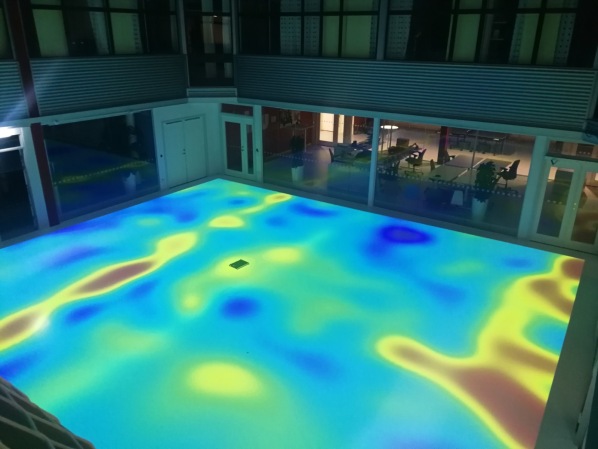
Figure 1: Illustration of the magnetic-field magnitude variations inside a building. The field near the floor was measured with a magnetometer, whose location was tracked by camera-based tracking systems. The field measurement was then interpolated, and the field magnitude was projected on the floor.

Indeed, recent years have witnessed many successful applications in magnetic-field-based positioning, among which the magnetic-field-based SLAM has turned out to be a promising approach[3, 4, 5]. It enables the user to construct a magnetic field map while navigating and having drift-free positioning, provided revisiting the same region is possible. However, this technology relies heavily on the precision of the used odometric information. Otherwise, the position drift can be significant, making it challenging to reliably recognize the visited place and complete “loop closure”[6]. For instance, when an inertial navigation system with low-cost inertial sensors is used for doing the odometry, the error growth rate is typically on the order of 10 meters per minute [7], which means the system needs to revisit the same region within a minute to prevent the position drift from becoming too large to complete loop closure. Therefore, the permissible length of the exploration phases where new areas are mapped is extremely limited when using low-cost inertial sensors. Hence, to increase the usability of current magnetic-field-based SLAM solutions we need robust odometry techniques that have a low position drift rate.

With this limitation in mind, the concept of combining inertial measurements and distributed magnetometry has been proposed and realized [8]. An array of magnetometers enables the calculation of the gradients of the magnetic field, from which the body velocity can be estimated. On the other hand, the authors in [2] adopted a model-based approach, treating pose changes in subsequent timestamps as the parameters of the model to be estimated. The estimated pose change from the magnetic field measurements can be used to aid an inertial navigation system to reduce the position growth rate. In this paper, we present a method for tightly integrated magnetic-field-aided inertial navigation. The resulting navigation system has, compared to a pure inertial navigation system, a significantly reduced error growth rate. Hence, the proposed navigation method has the potential to greatly extend the allowable length of the exploration phases in magnetic-field-based SLAM systems.

I-A Related Work

Numerous methods for magnetic-field-based indoor positioning and navigation have been proposed. Current solutions are roughly categorized into three types: fingerprint-based methods, magnetic field SLAM, and magnetic field odometry. Fingerprint-based methods[9, 10, 11] generally rely on a premeasured magnetic field map to work, which greatly limits its usability. Therefore, we mainly discuss the latter two types, which are not constrained by a prior map.

One of the first 2D magnetic field SLAM methods was proposed in [12], where the magnetic field strength map was constructed in hierarchical hexagonal tiles of different bin sizes. To generalize the motions to 3D and cope with the complexity of representing the map, the authors in [3] selected a reduced-rank Gaussian process to represent the magnetic field map and used a Rao-blackwellized particle filter to estimate both the map and the location of the system. Later, in [5], the authors successfully achieved drift-free positioning using foot-mounted sensors with similar techniques. To achieve real-time processing, they used an EKF filter to update the magnetic field map based on its gradients[4]. Contrary to the “stochastic” loop closure mechanism in [3, 5, 4], where it reduces the uncertainty of the map in the revisited region, a “deterministic” one was employed in [13], where attitude-invariant magnetic field information was used to detect loop closure and constraints on position estimates were formed. The aforementioned magnetic field SLAM solutions can achieve drift-free long-term large-scale positioning as long as frequent loop closure is possible.

Magnetic field odometry, on the other hand, is a lightweight solution to provide odometric information with a magnetometer array. It does not construct a magnetic field map but provides odometric information based on local magnetic field properties. The seminal work [8] derived an equation that relates the body velocity and the gradient of the magnetic field, which can be calculated from the measurements from a set of spatially distributed magnetometers. Later, in [14, 15], the authors proposed an observer to estimate body velocity, proved its convergence, and showcased its usability for indoor localization. In subsequent works [16, 17], the authors incorporated inertial sensor biases and magnetic disturbance in the model and designed a filter based on the error-state Kalman filter (ESKF). To address the issue of the noisy magnetic field gradient, the authors in [18, 19] derived a differential equation for high-order derivatives of the magnetic field. They then developed a filtering algorithm comprising a primary filter which is used to estimate the gradient of the field. Later, the same authors [20, 21] proposed an AI-based solution where a Long Short-Term Memory (LSTM) model is used to create a pseudo-measurement of the inertial velocity of the target. The pseudo-measurement is used to handle adversarial situations where the states’ observability is affected by the low gradient of the field and/or the target’s velocity close to zero. The methods developed have demonstrated promising prospects in magnetic field odometry. However, they are susceptible to noise when computing the gradient, and observability issues arise from a weak magnetic field gradient or low target speed. To address this problem, [22] matches the waveforms from a pair of magnetometers in a sliding time window to reduce the influence of the temporary disappearance of the magnetic field gradient. Experiments show that the proposed method in [22] performs similarly to wheel odometry in magnetic-rich environments.

In a more recent work [23], a polynomial model was proposed to describe the local magnetic field and to develop a magnetic field odometry method. Presented experiential results showed that the model-based odometry approach can give a higher accuracy at low signal-to-noise ratios, compared to approaches in [8]. The model-based odometry approach was further explored in [2], where it was used to estimate both the translation and orientation change of the array. In the subsequent work [24], the authors included the magnetic field model in the state-space description of an INS system and developed a tightly-integrated magnetic-field-aided INS. Simulation results showed that it has a much slower drift rate than stand-alone INS.

I-B Contributions

The contribution of this work is two-fold. Firstly, it extends the groundwork laid out in [24] by providing a thorough derivation and a comprehensive exposition of the proposed algorithm. Additionally, the performance of the proposed algorithm using real-world data was assessed and benchmarked against the state-of-the-art. Secondly, we have made the datasets used in our experiments and the source code for the proposed algorithm MAINS publicly available, in the hope that it will facilitate further research within the area of magnetic-field-based positioning. Both the datasets and the source code are available at https://github.com/Huang-Chuan/MAINSvsMAGEKF.

II System Modeling

Consider the problem of estimating the position and orientation of the sensor platform in Fig. 2, which consists of an inertial measurement unit (IMU) and an array of 30 magnetometers. To that end, a state-space model will be presented to realize a tightly-integrated magnetic-field aided inertial navigation system (INS).

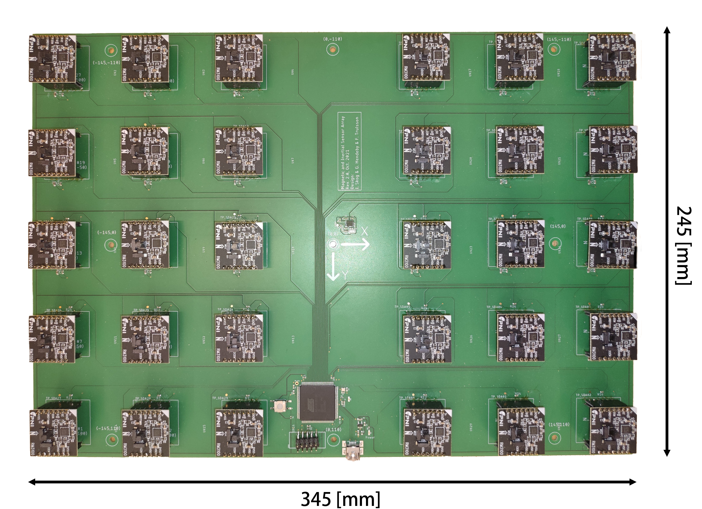
Figure 2: The sensor board used in the experiment. It has 30 PNI RM3100 magnetometers and an Osmium MIMU 4844 IMU mounted on the bottom side.

II-A Inertial Navigation Equations

Let the INS navigation state $x^{\text{\tiny{ins}}}_{k}$, the inertial measurements $\tilde{u}_{k}$, and the process noise $w^{\text{\tiny{ins}}}_{k}$ be defined as

$$x^{\text{\tiny{ins}}}_{k}\triangleq\begin{bmatrix}p_{k}^{n}\\ v_{k}^{n}\\ q_{k}\\ o^{a}_{k}\\ o^{\omega}_{k}\\ \end{bmatrix},\quad\tilde{u}_{k}\triangleq\begin{bmatrix}\tilde{s}_{k}\\ \tilde{\omega}_{k}\end{bmatrix},\quad\text{and}\quad w^{\text{\tiny{ins}}}_{k}\triangleq\begin{bmatrix}w_{k}^{a}\\ w_{k}^{\omega}\\ w_{k}^{o^{a}}\\ w_{k}^{o^{\omega}}\end{bmatrix},$$ (1)

respectively. Here, $p^{n}_{k}\in\mathbb{R}^{3}$, $v^{n}_{k}\in\mathbb{R}^{3}$, and $q_{k}\in\mathbb{H}$ denote the position, velocity, and orientation (parameterized as a unit quaternion) at time $k$, respectively. The superscript $n$ indicates that the vector is represented in the navigation frame. Moreover, $o^{a}_{k}\in\mathbb{R}^{3}$ and $o^{\omega}_{k}\in\mathbb{R}^{3}$ denote the accelerometer and gyroscope bias, respectively. Further, $\tilde{s}_{k}$ and $\tilde{\omega}_{k}$ denote the accelerometer and gyroscope measurements, respectively. Lastly, $w_{k}^{a}$ and $w_{k}^{\omega}$ denote the accelerometer and gyroscope measurement noise, respectively, and $w_{k}^{o^{a}}$ and $w_{k}^{o^{\omega}}$ denote the random walk process noise for the accelerometer and gyroscope biases, respectively. For an INS that uses low-cost sensors and moves at moderate velocities such that the effects of the transport rate, earth rotation, etc., can be neglected, the navigation equations are given by [25]

$$x^{\text{\tiny{ins}}}_{k+1} =f^{\text{\tiny{ins}}}(x^{\text{\tiny{ins}}}_{k},\tilde{u}_{k},w^{\text{\tiny{ins}}}_{k}),$$ (2a)

where

$$f^{\text{\tiny{ins}}}(x^{\text{\tiny{ins}}}_{k},\tilde{u}_{k},w^{\text{\tiny{ins}}}_{k})\!=\!\begin{bmatrix}p_{k}^{n}+v_{k}^{n}T_{s}+(R^{n}_{b_{k}}s_{k}+g^{n})\frac{T_{s}^{2}}{2}\\ v_{k}^{n}+(R^{n}_{b_{k}}s_{k}+g^{n})T_{s}\\ q_{k}\otimes\text{exp}_{q}\left(\omega_{k}T_{s}\right)\\ o^{a}_{k}+w_{k}^{o^{a}}\\ o^{\omega}_{k}+w_{k}^{o^{\omega}}\\ \end{bmatrix},$$ (2b)

and

$$s_{k} =\tilde{s}_{k}-o_{k}^{a}-w_{k}^{a},$$ (2c)

$$\omega_{k} =\tilde{\omega}_{k}-o_{k}^{\omega}-w_{k}^{\omega}.$$ (2d)

Here, the subscript $b_{k}$ denotes the body frame at time $k$, and $R^{n}_{b_{k}}\in\mathbb{SO}(3)$ denotes the rotation matrix that rotates a vector from the $b_{k}$-frame to the $n$-frame. Further, $T_{s}$ denotes the sampling period. Moreover, $s_{k}\in\mathbb{R}^{3}$ and $\omega_{k}\in\mathbb{R}^{3}$ denote the specific force and angular velocity, respectively. The vector $g^{n}\in\mathbb{R}^{3}$ denotes the local gravity. Furthermore, $\otimes$ denotes quaternion multiplication, and $\text{exp}_{q}(\cdot)$ is the operator that maps an axis-angle to a quaternion. Lastly, $w^{\text{\tiny{ins}}}_{k}$ is modeled as a zero-mean white Gaussian noise process with covariance matrix $\Sigma_{w^{\text{\tiny{ins}}}_{k}}=\text{blkdiag}(\Sigma_{a},\Sigma_{\omega},\Sigma_{o^{a}},\Sigma_{o^{\omega}})$, where $\Sigma_{(\cdot)}$ denotes the covariance matrix of the corresponding noise component and blkdiag($\cdot$) is an operator that creates a block diagnal matrix.

II-B Magnetic Field Modeling

The magnetic field is a three-dimensional vector field whose properties are described by Maxwell’s equations. Let $M(r;\theta)$ be a model of the magnetic field at the location $r\in\mathbb{R}^{3}$, parameterized by the parameter $\theta$. When there is no free current in the space $\Omega$, the magnetic-field model $M(r;\theta)$ should fulfill

$$\nabla_{r}\times M(r;\theta) =0,$$ (3a)

$$\nabla_{r}\cdot M(r;\theta) =0,$$ (3b)

for all $r\in\Omega$. A polynomial magnetic field model, which fulfills (3), is given by [23]

$$M(r;\theta)=\Phi(r)\theta.$$ (4)

Here $\Phi(r)\in\mathbb{R}^{3\times\kappa}$ is the regression matrix defined in [23] and $\theta\in\mathbb{R}^{\kappa}$ is the coefficient of the polynomial model; for a $n^{\text{th}}$ order polynomial the model has $\kappa$ = dim($\theta$) = $n^{2}+4n+3$ unknown parameters[2]. Note that the model (4) can be defined in either the body frame or navigation frame. Within this paper, it will be defined in the body frame. Next, a procedure for transforming the model from the $b_{k}$ frame to the $b_{k+1}$ frame will be presented.

Let the magnetic field model (4) be associated with the $b$-frame, which means $M(r;\theta)$ accepts locations $r$ expressed in $b$-frame and outputs magnetic field vector in the same frame. Then $M_{k}(r;\theta_{k})$ denotes the magnetic field model associated with the $b_{k}$-frame, i.e.,

$$M_{k}(r^{b_{k}};\theta_{k})=\Phi(r^{b_{k}})\theta_{k}.$$ (5)

When the body frame moves, the coefficient $\theta_{k}$ evolves over time along with the changes in the body frame. Let the relative body frame change from $b_{k}$ to $b_{k+1}$ be encoded by

$$\psi_{k}=\begin{bmatrix}\Delta p_{k}\\ \Delta\phi_{k}\end{bmatrix},$$ (6)

where ${\Delta p}_{k}\in\mathbb{R}^{3}$ and $\Delta\phi_{k}\in[0,2\pi]^{3}$ denote the translation and orientation change from the body frame $b_{k}$ to $b_{k+1}$, respectively. Then the dynamics of $\theta_{k}$ can be found by expressing the magnetic field vector at a given location with the models at two consecutive times and aligning them in the same frame. The basic idea is illustrated in Fig. 3, from which the following two equalities can be identified

$$M_{k+1}(r^{b_{k+1}};\theta_{k+1}) =R_{b_{k}}^{b_{k+1}}M_{k}(r^{b_{k}};\theta_{k}),$$ (7a)

$$r^{b_{k}} =(R_{b_{k}}^{b_{k+1}})^{\top}r^{b_{k+1}}+{\Delta p}_{k}.$$ (7b)

Here $R_{b_{k}}^{b_{k+1}}$ denotes the rotation matrix that rotates a vector from the $b_{k}$-frame to the $b_{k+1}$-frame. The rotation matrix $R_{b_{k}}^{b_{k+1}}$ and translation $\Delta p_{k}$ are given by

$$R_{b_{k}}^{b_{k+1}}=\left(\text{exp}(\left[\Delta\phi_{k}\right]_{\times})\right)^{\top}=\left(\text{exp}(\left[\omega_{k}T_{s}\right]_{\times})\right)^{\top},$$ (8a)

$$\Delta p_{k}=R_{b_{k}}^{n^{\top}}\left(v_{k}^{n}T_{s}+(R^{n}_{b_{k}}s_{k}+g^{n})\frac{T_{s}^{2}}{2}\right).$$ (8b)

Here $[\cdot]_{\times}$ is an operator that maps a vector in $\mathbb{R}^{3}$ to a skew-symmetric matrix such that $\left[a\right]_{\times}b=a\times b$.

Figure 3: A 2D illustration of the geometric relationship between the body frames at two consecutive times. The applicable region $\Omega$ of the magnetic field model at time $k$ is in blue, and the black dot indicates the location where the two models output the corresponding magnetic field in their own coordinate frames.

Substituting the generic magnetic model in (7) with the proposed polynomial model (5) yields the equality

$$\Phi(r^{b_{k+1}})\theta_{k+1}=R_{b_{k}}^{b_{k+1}}\Phi(r^{b_{k}})\theta_{k}.$$ (9)

Note that for a given $r^{b_{k+1}}$, $\theta_{k}$ and $\psi_{k}$, (9) represents 3 linear equations. Since $\theta_{k+1}$ is of dimension $\kappa$, which is greater than 3, it is necessary to use more than one location vector $r$ to solve the equation system. In general, $S=\lceil\kappa/3\rceil$ location vectors can be used to construct the equation system, i.e.,

$$\underbrace{\begin{bmatrix}\Phi(r^{b_{k+1}}_{1})\\ \vdots\\ \Phi(r^{b_{k+1}}_{S})\\ \end{bmatrix}}_{\triangleq A}\theta_{k+1}=\underbrace{\begin{bmatrix}R_{b_{k}}^{b_{k+1}}\Phi(r^{b_{k}}_{1})\\ \vdots\\ R_{b_{k}}^{b_{k+1}}\Phi(r^{b_{k}}_{S})\\ \end{bmatrix}}_{\triangleq B(\psi_{k})}\theta_{k}.$$ (10)

Note that the location vectors $r^{b_{k+1}}_{1},\cdots,r^{b_{k+1}}_{S}$ can be chosen such that $A$ has full column rank, and they are fixed. Finally, it holds that

$$\theta_{k+1}=A^{\dagger}B(\psi_{k})\theta_{k},$$ (11)

where $A^{\dagger}$ denotes the Moore–Penrose inverse of $A$.

Since the magnetic field model should describe the magnetic field locally, the update in (11), which implicitly expands the applicable space $\Omega$ of the model, will inevitably introduce additional modeling errors. To account for those errors, with a slight abuse of notation, the update of the polynomial coefficients of the magnetic field as the body frame change is modeled as

$$\theta_{k+1}=A^{\dagger}B(\psi_{k})\theta_{k}+w^{\theta}_{k},$$ (12)

where $w_{k}^{\theta}$ is assumed to be a white Gaussian noise process with zero mean and covariance matrix $\Sigma_{\theta}$. Hence, the dynamic model for the magnetic-field subsystem is

$$\theta_{k+1}=f^{\theta}(\theta_{k},x^{\text{\tiny{ins}}}_{k},\tilde{u}_{k},w^{\text{\tiny{ins}}}_{k},w^{\theta}_{k}),$$ (13)

where

$$f^{\theta}(\theta_{k},x^{\text{\tiny{ins}}}_{k},\tilde{u}_{k},w^{\text{\tiny{ins}}}_{k},w^{\theta}_{k})=A^{\dagger}B(\psi_{k})\theta_{k}+w^{\theta}_{k}.$$ (14)

Note that $\psi_{k}$ is a function of $x^{\text{\tiny{ins}}}_{k}$, $\tilde{u}_{k}$, and $w^{\text{\tiny{ins}}}_{k}$.

II-C Magnetometer Array Measurement Model

Given the magnetic field model in (5), the measurement $y_{k}^{(i)}\in\mathbb{R}^{3}$ from the $i^{\text{th}}$ sensor in the magnetometer array at time $k$ can be modeled as

$$y_{k}^{(i)}=\Phi(r_{m_{i}})\theta_{k}+e_{k}^{(i)},$$ (15)

where $r_{m_{i}}\in\mathbb{R}^{3}$ denotes the location of the $i^{\text{th}}$ magnetometer in the array. Further, $e_{k}^{(i)}\in\mathbb{R}^{3}$ denotes the measurement error, which includes both the measurement noise and the imperfections of the magnetic-field model. The error is assumed to be white and Gaussian distributed with covariance matrix $\Sigma_{e_{k}^{(i)}}$.

II-D Complete System

Given the presented navigation equations and the magnetic-field model, the dynamics and observations of the full system can be described by the following state-space model.

Let the state vector $x_{k}$, the process noise vector $w_{k}$, and the measurement noise $e_{k}$ be defined as

$$x_{k}\triangleq\begin{bmatrix}x^{\text{\tiny{ins}}}_{k}\\ \theta_{k}\end{bmatrix},\quad w_{k}\triangleq\begin{bmatrix}w_{k}^{\text{\tiny{ins}}}\\ w_{k}^{\theta}\end{bmatrix},\quad\text{and}\quad e_{k}\triangleq\begin{bmatrix}e_{k}^{(1)}\\ \vdots\\ e_{k}^{(N)}\\ \end{bmatrix},$$ (16)

respectively. Combining the models in (2), (13), and (15) gives the state-space model

$$x_{k+1} =f(x_{k},\tilde{u}_{k},w_{k}),$$ (17a)

$$y_{k} =Hx_{k}+e_{k},$$ (17b)

where

$$f(x_{k},\tilde{u}_{k},w_{k})=\begin{bmatrix}f^{\text{\tiny{ins}}}(x^{\text{\tiny{ins}}}_{k},\tilde{u}_{k},w^{\text{\tiny{ins}}}_{k})\\ f^{\theta}(\theta_{k},x^{\text{\tiny{ins}}}_{k},\tilde{u}_{k},w^{\theta}_{k})\end{bmatrix},$$ (17c)

and

$$H=\begin{bmatrix}0&\Phi(r_{m_{1}})\\ \vdots&\vdots\\ 0&\Phi(r_{m_{N}})\\ \end{bmatrix}.$$ (17d)

Here, the process noise covariance $$Q_{k} R_{k}$$ and the measurement noise covariance are

$$Q_{k} \triangleq\textbf{Cov}(w_{k})=\text{blkdiag}(\Sigma_{a},\Sigma_{\omega},\Sigma_{o^{a}},\Sigma_{o^{\omega}},\Sigma_{\theta}),$$ (17e)

$$R_{k} \triangleq\textbf{Cov}(e_{k})=\text{blkdiag}(\Sigma_{e_{k}^{(1)}},\Sigma_{e_{k}^{(2)}},\cdots,\Sigma_{e_{k}^{(N)}}),$$ (17f)

respectively.

III State Estimation

The quaternion $q_{k}$ in the state vector does not belong to Euclidean space. Therefore, standard nonlinear filter algorithms, such as the extended Kalman filter and unscented Kalman filter, cannot be applied to the state-space model in (17) without appropriate modifications. The error state Kalman filter (ESKF) presented in [25] circumvents the problem by the use of “error quaternion”, which is a small perturbation around the “estimated quaternion” expressed in $\mathbb{R}^{3}$. With reference to Fig. 4, the algorithm works by propagating an estimated state $\hat{x}_{k}$ via the state transition model in (17a) and using a complementary Kalman filter to estimate the error state $\delta x_{k}$, which is then used to correct the estimated state $\hat{x}_{k}$. Since the ESKF is a standard algorithm, only the error propagation model that is unique to the state-space model in (17), will here be derived.

Figure 4: The flowchart of the state estimation algorithm.

III-A Error State Definition

The error state $\delta x_{k}$ is defined as

$$\delta x_{k}\triangleq\begin{bmatrix}\delta x^{\text{\tiny{ins}}}_{k}\\ \delta\theta_{k}\end{bmatrix}\quad\text{and}\quad\delta x^{\text{\tiny{ins}}}_{k}=\begin{bmatrix}\delta p_{k}^{n}\\ \delta v_{k}^{n}\\ \epsilon_{k}\\ \delta o_{k}^{a}\\ \delta o_{k}^{\omega}\\ \end{bmatrix}.$$ (18)

Here, for the position, velocity, sensor biases, and magnetic field model parameters, the standard additive error definition is used (e.g., $\delta p_{k}^{n}=p^{n}_{k}-\hat{p}_{k}^{n}$). On the other hand, the orientation error $\epsilon_{k}\in\mathbb{R}^{3}$ satisfies the equation $R_{b_{k}}^{n}\simeq\hat{R}_{b_{k}}^{n}(I_{3}+[\epsilon_{k}]_{\times})$. The true state $x_{k}$ and the estimated state $\hat{x}_{k}$ relate to each other via

$$x_{k}=\hat{x}_{k}\oplus\delta x_{k},$$ (19)

where the operator $\oplus$ is defined by

$$p^{n}_{k} =\hat{p}_{k}^{n}+{\delta p_{k}^{n}},$$ (20a)

$$v^{n}_{k} =\hat{v}^{n}_{k}+{\delta v^{n}_{k}},$$ (20b)

$$q_{k} =\hat{q}_{k}\otimes[1\quad\frac{1}{2}\epsilon_{k}^{\top}]^{\top},$$ (20c)

$$o_{k}^{a} =\hat{o}_{k}^{a}+\delta o_{k}^{a},$$ (20d)

$$o_{k}^{\omega} =\hat{o}^{\omega}_{k}+\delta o_{k}^{\omega},$$ (20e)

$${\theta}_{k} =\hat{\theta}_{k}+{\delta\theta_{k}}.$$ (20f)

III-B Inertial Error State Dynamics

The dynamics of $\delta x^{\text{\tiny{ins}}}_{k}$ has been derived in [25] and are given by

$$\delta x^{\text{\tiny{ins}}}_{k+1}=F^{\text{\tiny{ins}}}_{k}\delta x^{\text{\tiny{ins}}}_{k}+G^{\text{\tiny{ins}}}_{k}w^{\text{\tiny{ins}}}_{k},$$ (21a)

where

$$F^{\text{\tiny{ins}}}_{k}=\begin{bmatrix}I_{3}&I_{3}T_{s}&0&0&0\\ 0&I_{3}&-\hat{R}_{b_{k}}^{n}[\hat{s}_{k}]_{\times}T_{s}&-\hat{R}_{b_{k}}^{n}T_{s}&0\\ 0&0&\text{exp}([\Delta\hat{\phi}_{k}]_{\times})^{\top}&0&-I_{3}T_{s}\\ 0&0&0&I_{3}&0\\ 0&0&0&0&I_{3}\end{bmatrix},$$ (21b)

$$G^{\text{\tiny{ins}}}_{k} =\begin{bmatrix}0&0&0&0\\ \hat{R}_{b_{k}}^{n}T_{s}&0&0&0\\ 0&I_{3}T_{s}&0&0\\ 0&0&I_{3}\sqrt{T_{s}}&0\\ 0&0&0&I_{3}\sqrt{T_{s}}\end{bmatrix}.$$ (21c)

Here, $$\hat{s}_{k}=\tilde{s}_{k}-\hat{o}^{a}_{k} \Delta\hat{\phi}_{k}=(\tilde{\omega}_{k}-\hat{o}^{\omega}_{k})T_{s}$$ and .

III-C Magnetic Field Subsystem Error State Dynamics

To the first order, the errors in (13) propagate according to

$$\delta\theta_{k+1}=A^{\dagger}\begin{bmatrix}B(\hat{\psi_{k}})&\frac{d}{d\psi_{k}}\bigl{(}B(\hat{\psi}_{k})\theta_{k}\bigr{)}\end{bmatrix}\begin{bmatrix}\delta\theta_{k}\\ \delta\psi_{k}\end{bmatrix}\\ +w_{k}^{\theta},$$ (22a)

where

$$\delta\psi_{k}=\psi_{k}-\hat{\psi}_{k}.$$ (22b)

However, instead of expressing the error development in terms of $\delta\psi_{k}$, we would like to express it in terms of the orientation error $\epsilon_{k}$, velocity error $\delta v^{n}_{k}$, accelerometer bias estimation error $\delta o_{k}^{a}$, and gyroscope bias estimation error $\delta o_{k}^{\omega}$. To do so, note that from (8b) we have

$$\begin{split}\Delta\hat{p}_{k}&=\hat{R}^{b_{k}}_{n}T_{s}(\hat{v}^{n}_{k}+g^{n}T_{s}/2)+\hat{s}_{k}T^{2}_{s}/2,\end{split}$$ (23a)

where

$$\hat{R}^{b_{k}}_{n}=(I_{3}-[\epsilon_{k}]_{\times})^{-1}R^{b_{k}}_{n},$$ (23b)

which gives that

$$\begin{split}\delta\Delta p_{k}=&\Delta p_{k}-\Delta\hat{p}_{k}\\ \approx&-[\epsilon_{k}]_{\times}\hat{R}^{b_{k}}_{n}T_{s}(\hat{v}^{n}_{k}+g^{n}T_{s}/2)+\hat{R}^{b_{k}}_{n}\delta v^{n}_{k}T_{s}\\ =&[\underbrace{\hat{R}^{b_{k}}_{n}T_{s}(\hat{v}^{n}_{k}+g^{n}T_{s}/2)}_{\eta(\hat{R}^{b_{k}}_{n},\hat{v}^{n}_{k})}]_{\times}\epsilon_{k}+\hat{R}^{b_{k}}_{n}\delta v^{n}_{k}T_{s}.\end{split}$$ (24)

Here, the second and higher-order error terms have been neglected. Moreover, it holds that

$$\delta\phi_{k}=\Delta\phi_{k}-\Delta\hat{\phi}_{k}=-(\delta o_{k}^{\omega}+w_{k}^{\omega})T_{s}.$$ (25)

Bringing it all together gives the following expression for the magnetic field subsystem error state propagation

$$\delta\theta_{k+1}=F^{\theta}_{k}\delta\hat{x}_{k}+G^{\theta}_{k}w^{\theta}_{k},$$ (26a)

where

$$F^{\theta}_{k} = A^{\dagger}\begin{bmatrix}B(\hat{\psi}_{k})&J_{1}&J_{2}\end{bmatrix}C(\hat{x}_{k}),$$ (26b)

$$G^{\theta}_{k}=\begin{bmatrix}0\quad-J_{2}T_{s}\quad I_{\kappa}\end{bmatrix}.$$ (26c)

Here,

$$J_{1} = \frac{d}{d\Delta p_{k}}\bigl{(}B(\hat{\psi}_{k})\theta_{k}\bigr{)},$$ (26d)

$$J_{2} = \frac{d}{d\Delta\phi_{k}}\bigl{(}B(\hat{\psi}_{k})\theta_{k}\bigr{)},$$ (26e)

and

$$\!C(\hat{x}_{k})\!=\!\begin{bmatrix}0&\!0&\!0&\!0&\!0&\!I_{\kappa}\\ 0&\!\hat{R}^{b_{k}}_{n}T_{s}&\![\eta(\hat{R}^{b_{k}}_{n},\hat{v}^{n}_{k})]_{\times}&\!0&\!0&\!0\\ 0&\!0&\!0&\!0&\!-I_{3}T_{s}&\!0\end{bmatrix}.$$ (26f)

Combining (21) and (26) gives the complete state-space description for the error state, i.e.,

$$\delta x_{k+1} =F_{k}\delta x_{k}+G_{k}w_{k},$$ (27a)

$$y_{k} =H(\hat{x}_{k}\oplus\delta x_{k})+e_{k},$$ (27b)

where

$$F_{k}=\begin{bmatrix}F^{\text{\tiny{ins}}}_{k}&0\\ \lx@intercol\hfil F^{\theta}_{k}\hfil\lx@intercol\end{bmatrix},\quad G_{k}=\begin{bmatrix}G^{\text{\tiny{ins}}}_{k}\\ G^{\theta}_{k}\end{bmatrix}.$$ (27c)

The Kalman filter can be applied to (27) to estimate the error state, which is then used to correct the estimated state. The complete description of the proposed ESKF is summarized in Algorithm 1.

Algorithm 1 ESKF algorithm

0:  $\{\tilde{u}_{k},y_{k}\}_{k=0}^{N}$

0:  $\{\hat{x}_{k|k},P_{k|k}\}_{k=1}^{N}$ Initialisation : estimated state $\hat{x}_{0|0}$, covariance matrix $P_{0|0}$

  For $k=0$ to $N-1$ do

       State propagation

       $\hat{x}_{k+1|k}\leftarrow f(\hat{x}_{k|k},\tilde{u}_{k},0)$

       Error state uncertainty propagation

       $P_{k+1|k}\leftarrow F_{k}P_{k|k}F_{k}^{\top}+G_{k}Q_{k}G^{\top}$

       Error state observation

       $z_{k+1}\leftarrow y_{k+1}-H\hat{x}_{k+1}$

       $S_{k+1}\leftarrow HP_{k+1|k}H^{\top}+R_{k+1}$

       $K_{k+1}\leftarrow P_{k+1|k}H^{\top}S_{k+1}^{-1}$

       $\delta\hat{x}_{k+1}\leftarrow K_{k+1}z_{k+1}$

       $P_{k+1|k+1}\leftarrow P_{k+1|k}-K_{k+1}HP_{k+1|k}$

       Correct the estimated state

       $\hat{x}_{k+1|k+1}\leftarrow\hat{x}_{k+1|k}\oplus\delta\hat{x}_{k+1}$

       ESKF reset

       $\delta\hat{x}_{k+1}\leftarrow 0$

  end for

III-D Adaptation of the measurement noise covariance

As previously mentioned, the polynomial magnetic field model is not perfect. The model imperfections will vary with the complexity of the magnetic field and the covariance $R_{k}$ should vary accordingly. One possibility to make $R_{k}$ adapt to the complexity of the field is to assume $R_{k}=\sigma_{k}^{2}I_{3N}$ and then fit the magnetic-field model to the current observations $y_{k}$ and estimate $\sigma_{k}^{2}$ from the residual. That is, $\sigma_{k}^{2}$ is estimated as [26],

$$\hat{\sigma}^{2}_{k}=\frac{1}{3N}\lVert(I_{3N}-XX^{\dagger})y_{k}\rVert^{2},$$ (28a)

where $$X$$ is given by

$$X=\begin{bmatrix}\Phi(r_{m_{1}})\\ \vdots\\ \Phi(r_{m_{N}})\end{bmatrix}.$$ (28b)

IV Experimental Results

To evaluate the proposed method multiple experiments were conducted using the array in Fig. 2. In each experiment, the magnetometer array was first sitting still on the ground for a few seconds and then picked up by a person. The person then held it in his/her hands and walked in squares for a few laps before putting the board back on the ground. The true trajectory of the array was measured using a camera-based motion-tracking system. In total 8 datasets were recorded. The main characteristics of the different datasets are summarized in Table I.

TABLE I: Information about the datasets

Data sequence	LP-1	LP-2	LP-3	NP-1	NP-2	NP-3	NT-1	NT-2
Trajectory length* (m)	138.72	167.07	194.41	136.23	134.66	137.76	164.62	137.87
Trajectory duration* (s)	272	286	332	177	165	154	185	151
Average height (m)	0.49	0.52	0.55	0.85	0.84	0.79	0.73	0.74
Board orientation relative to the ground	parallel	parallel	parallel	parallel	parallel	parallel	tilted	tilted

* including the initial part of the trajectory where the position-aiding is turned on.
LP: low height and parallel   NP: normal height and parallel   NT: normal height and tilted.

The datasets were processed with three algorithms: a stand-alone INS; the proposed MAINS, and the method proposed in [19]. The positions measured by the motion-tracking system were first made available to all algorithms for 60 seconds to calibrate IMU biases and stabilize state estimates. Then all systems operated without position aiding for the rest trajectory. This is similar to the scenario of a user coming into a building where GNSS signals are lost. Since the method in [19] by default is designed to use 5 magnetometers, the same sensor configuration (the left in Fig. 5) as in [19] was used when comparing the two algorithms; only the performance during the non-position-aiding part of the trajectory was evaluated. An example of the estimated trajectories estimated by the three algorithms and the corresponding positional errors are plotted in Fig. 6. Since MAINS supports using other sensor configurations than the square configuration, the performance of the proposed algorithm was also evaluated using all the sensors in the array (see Fig. 5). An example of the trajectory estimated when using all sensors is shown in Fig. 7. The results, in terms of root mean square (RMS) position and velocity errors, from processing all 8 datasets with the different sensor configurations and algorithms are summarized in Table II. The position errors at the end of the trajectories are also shown.

It can be seen from Fig. 6 that both MAINS and the method in [19] output a trajectory with a similar shape as the true trajectory, while the INS trajectory quickly drifted away. The same conclusion can be drawn from the horizontal and vertical error plots. As expected the position error of the INS grows much faster than those of the other two methods. Looking at the results in Tab. II, it shows that both MAINS and the method [19] achieved superior performance in terms of horizontal error, vertical error, and speed error, compared to the stand-alone INS. However, MAINS has a consistently lower speed error than the method [19] on all datasets. Furthermore, MAINS has, in general, a lower average horizontal error, which is consistent with the observation of the trajectory shown in Fig. 6. In terms of vertical error, the method [19] performed poorly on the datasets where the board was tilted, while MAINS had larger errors on the datasets where the board was close to the ground. The reason for [19] performing worse is that when the board is tilted (so is the body frame), the speed errors in all three axes contributed to a larger vertical error, compared to the case when the board is flat and the vertical error comes mostly from the speed error in the z-axis. Meanwhile, the reason why MAINS produced trajectories with a large vertical drift when the board was close to the ground is that the magnetic field there was too complex for the polynomial model, which results in large fitting residuals and thus large innovations in filtering pulling the estimate away from what it should be. Comparing the performance of the MAINS algorithm with the two different sensor configurations, the benefit of using more sensors is apparent — Vertical error was significantly reduced, and both the horizontal and vertical error at the end of the trajectory were less than 3 meters for most trajectories.

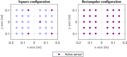
Figure 5: Sensor configurations used in the experiments. Left: Square configuration. Right: Rectangular configuration.

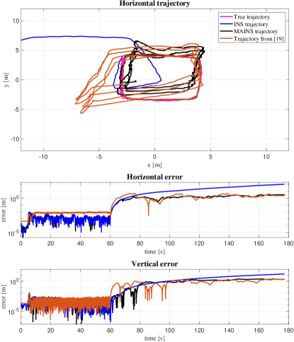
Figure 6: Estimated trajectory and the corresponding positional errors from a stand-alone INS, MAINS, and the method proposed in [19]. The square sensor configuration was used in this experiment.

To help readers better understand the magnetic field in which the experiments were conducted and the full potential of MAINS, the trajectory estimated by MAINS with rectangular sensor configuration is plotted on top of a magnetic field magnitude plot, as shown in Fig. 7. It can be seen that the magnitude variance along the trajectory is around 8 $\mu$T, and the gradient varies. MAINS is capable of producing a trajectory that is very close to the true one, and more importantly, the positional error is consistently reflected by the uncertainty. One thing that may raise readers’ interest is why the trajectory seems to always “bend inwards” near the top left corner. We cannot offer a precise explanation now, but one of the possibilities is that MAINS is sensitive to errors in magnetometer calibration parameters, which are difficult to eliminate.

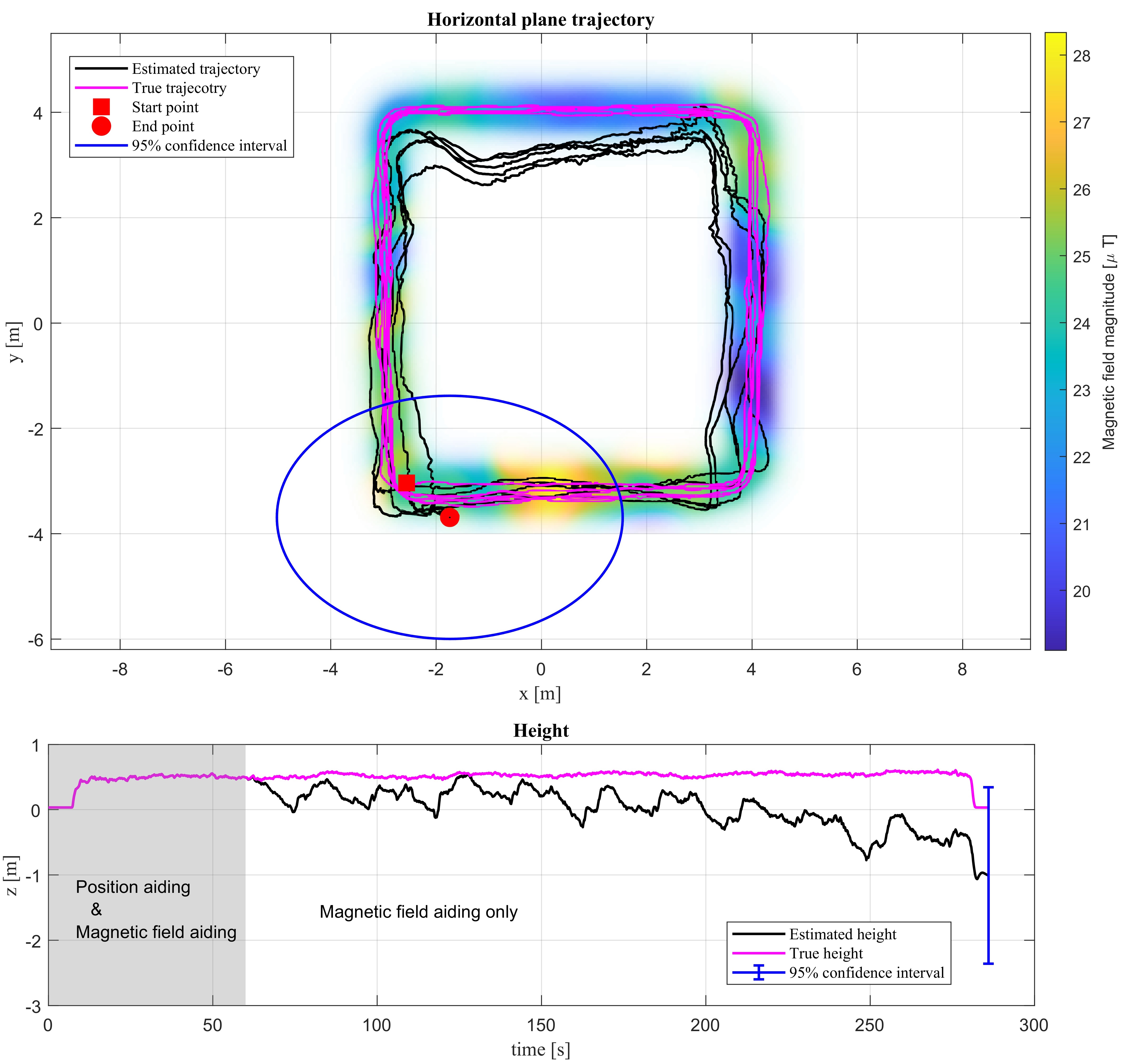
Figure 7: Illustration of the estimated and the true trajectory, as well as the magnetic field magnitude along the trajectory. The magnetic field magnitude plot is created by the interpolated magnetic field measurements using a Gaussian process model.

TABLE II: Summary of results from experimental evaluation

	LP-1	LP-2	LP-3	NP-1	NP-2	NP-3	NT-1	NT-2
Trajectory length* (m)	114.14	139.87	162.30	93.68	89.47	86.43	123.01	87.26
Trajectory duration* (s)	212	226	272	117	105	94	125	91
Stand-alone INS
RMS Horizontal Error (m)	45.18	140.04	384.41	43.92	28.14	36.0	130.27	36.91
Horizontal Error at the end (m)	75.48	346.84	1090.47	108.53	77.02	84.27	300.99	90.84
RMS Vertical Error (m)	87.13	78.45	110.54	6.48	10.77	5.08	5.72	10.76
Vertical Error at the end (m)	206.12	183.6	256.96	16.02	24.73	12.07	11.09	25.9
RMS Speed Error (m/s)	1.84	2.44	5.96	1.29	1.06	1.09	2.86	1.3
The method [19] with the square sensor configuration in Fig. 5
RMS Horizontal Error (m)	2.16	2.61	3.02	2.38	3.88	1.43	4.3	1.18
Horizontal Error at the end (m)	3.89	4.42	5.15	2.44	5.79	1.56	7.15	0.98
RMS Vertical Error (m)	0.96	1.49	2.4	1.09	2.03	0.74	12.24	6.74
Vertical Error at the end (m)	2.0	2.73	4.25	2.0	3.39	0.68	20.6	10.96
RMS Speed Error (m/s)	0.35	0.51	0.58	0.63	0.51	0.56	0.49	0.50
MAINS with the square sensor configuration in Fig. 5
RMS Horizontal Error (m)	0.66	1.29	1.6	1.88	1.62	1.89	2.91	0.81
Horizontal Error at the end (m)	1.25	1.82	2.55	3.22	2.65	2.89	4.51	1.04
RMS Vertical Error (m)	5.59	6.32	6.87	1.42	0.58	1.16	1.27	0.74
Vertical Error at the end(m)	9.61	10.54	11.76	2.04	1.21	1.16	2.22	1.42
RMS Speed Error (m/s)	0.12	0.17	0.14	0.24	0.17	0.29	0.22	0.20
MAINS with the rectangular sensor configuration in Fig. 5
RMS Horizontal Error (m)	0.77	0.84	1.15	2.65	1.24	2.32	0.83	1.73
Horizontal Error at the end (m)	0.61	1.65	2.49	4.21	1.49	3.72	1.82	2.38
RMS Vertical Error (m)	0.49	0.57	0.74	2.09	0.35	2.11	1.91	0.25
Vertical Error at the end (m)	0.56	0.99	1.22	2.78	0.89	2.52	3.16	0.64
RMS Speed Error (m/s)	0.10	0.11	0.12	0.20	0.24	0.24	0.19	0.17

* excluding the initial part of the trajectory where the position-aiding is turned on.

V Conclusion and Future Work

The results presented in this paper demonstrate the effectiveness of the MAINS algorithm for magnetic-field-based indoor positioning. The proposed algorithm outperforms the stand-alone INS in terms of horizontal and vertical error, as well as speed error. Furthermore, it has a comparable performance with the state-of-the-art method with the same sensor configuration. Having the advantage of being flexible with sensor configurations, the MAINS algorithm can, in most cases, limit the position drift to less than 3 meters after 2 minutes of navigation when using all magnetometers.

Future work could focus on investigating loop closure detection mechanisms for magnetic field SLAM, unifying sensor calibration and parameter tuning within the MAINS framework, and exploring the impact of the magnetic field model on positioning error. Overall, the MAINS algorithm shows great promise for real-life applications of magnetic-field-based positioning.

Chuan Huang (Student member, IEEE) received the B.Sc. from Beihang University in 2018 and the M.Sc. degree from China Electronics Technology Group Corporation Academy of Electronics and Information Technology in 2021. He is now a Ph.D. student at Linköping university, Sweden. His main research interest is sensor fusion with applications to magnetic field based positioning.

Gustaf Hendeby (Senior member, IEEE) received the M.Sc. degree in applied physics and electrical engineering in 2002 and the Ph.D. degree in automatic control in 2008, both from Linkoping University, Linkoping, Sweden. He is Associate Professor and Docent in the division of Automatic Control, Department of Electrical Engineering, Linkoping University. He worked as Senior Researcher at the German Research Center for Artificial Intelligence (DFKI) 2009–2011, and Senior Scientist at Swedish Defense Research Agency (FOI) and held an adjunct Associate Professor position at Linkoping University 2011–2015. His main research interests are stochastic signal processing and sensor fusion with applications to nonlinear problems, target tracking, and simultaneous localization and mapping (SLAM), and is the author of several published articles and conference papers in the area. He has experience of both theoretical analysis as well as implementation aspects. Dr. Hendeby is since 2018 an Associate Editor for IEEE Transactions on Aerospace and Electronic Systems in the area of target tracking and multisensor systems. In 2022 he served as general chair for the 25th IEEE International Conference on Information Fusion (FUSION) in Linkoping, Sweden.

Hassen Fourati (Senior member, IEEE) received his bachelor of engineering degree in electrical engineering at the National Engineering School of Sfax (ENIS), Tunisia; master’s degree in automated systems and control at the University of Claude Bernard (UCBL), Lyon, France; and PhD degree in automatic control at the University of Strasbourg, France, in 2006, 2007, and 2010, respectively. He is currently an associate professor of the electrical engineering and computer science at the University of Grenoble Alpes, Grenoble, France, and a member of the Dynamics and Control of Networks Team (DANCE), affiliated to the Pôle Automatique et Diagnostic (PAD) of the GIPSA-Lab. His research interests include nonlinear filtering, estimation and multisensor fusion with applications in navigation, motion analysis, mobility and traffic management. He has published several research papers in scientific journals, international conferences, book chapters and books.

Christophe Prieur (Fellow member, IEEE) received the M.Sc. degree in mathematics from the École Normale Supérieure de Cachan, France, in 2000, and the Ph.D. degree in applied mathematics from Université Paris-Sud, Orsay, France, in 2001. He has been a Senior Researcher with the French National Centre for Scientific Research, Paris, France, since 2011. His current research interests include nonlinear control theory, hybrid systems, and control of partial differential equations. Dr. Prieur has been a member of the European Control Association-Conference Editorial Board (EUCA-CEB) and the IEEE-Control Systems Society (CSS) CEB. He was the Program Chair of the 9th IFAC Symposium on Nonlinear Control Systems (NOLCOS 2013) and the 14th European Control Conference (ECC 2015). He has been an Associate Editor of the IEEE Transactions on Automatic Control, the European Journal of Control, and the IEEE Transactions on Control Systems Technology. He is an Associate Editor of the Evolution Equations and Control Theory (AIMS) and the SIAM Journal on Control and Optimization. He is also a Senior Editor of the IEEE Control Systems Letters and an Editor of the IMA Journal of Mathematical Control and Information.

Isaac Skog (Senior Member, IEEE) received the B.Sc. and M.Sc. degrees in electrical engineering from the KTH Royal Institute of Technology, Stockholm, Sweden, in 2003 and 2005, respectively. In 2010, he received the Ph.D. degree in signal processing with a thesis on low-cost navigation systems. In 2009, he spent 5 months with the Mobile Multi-Sensor System Research Team, University of Calgary, Calgary, AB, Canada, as a Visiting Scholar and in 2011 he spent 4 months with the Indian Institute of Science, Bangalore, India, as a Visiting Scholar. Between 2010 and 2017, he was a Researcher with the KTH Royal Institute of Technology. He is currently an Associate Professor with Linköping University, Linköping, Sweden, and a Senior Researcher with Swedish Defence Research Agency (FOI), Stockholm, Sweden. He is the author and coauthor of more than 60 international journal and conference publications. He was the recipient of the Best Survey Paper Award by the IEEE Intelligent Transportation Systems Society in 2013.

References

- [1] C.-I. Chesneau, “Magneto-inertial dead-reckoning in inhomogeneous field and indoor applications,” Ph.D. dissertation, Université Grenoble Alpes, 2018.
- [2] I. Skog, G. Hendeby, and F. Trulsson, “Magnetic-field based odometry – an optical flow inspired approach,” in Int. Conf. on Indoor Positioning and Indoor Navigation (IPIN), Lloret de Mar, Spain, Nov. 2021, pp. 1–8.
- [3] M. Kok and A. Solin, “Scalable magnetic field SLAM in 3D using gaussian process maps,” in Proc. 2018 21st Int. Conf. on Information Fusion (FUSION), Cambridge, United Kingdom, July 2018, pp. 1353–1360.
- [4] F. Viset, R. Helmons, and M. Kok, “An extended Kalman filter for magnetic field slam using gaussian process regression,” Sensors, vol. 22, no. 8, 2022.
- [5] F. Viset, J. T. Gravdahl, and M. Kok, “Magnetic field norm SLAM using Gaussian process regression in foot-mounted sensors,” in European Control Conference (ECC), Rotterdam, Netherlands, June 2021, pp. 392–398.
- [6] S. Thrun, W. Burgard, and D. Fox, Probabilistic robotics. Cambridge, Mass.: MIT Press, 2005.
- [7] J.-O. Nilsson and I. Skog, “Inertial sensor arrays — a literature review,” in Proc. 2016 European Navigation Conference (ENC), Helsinki, Finland, May 2016, pp. 1–10.
- [8] D. Vissiere, A. Martin, and N. Petit, “Using distributed magnetometers to increase imu-based velocity estimation into perturbed area,” in Proc. 2007 46th IEEE Conference on Decision and Control, New Orleans, LA, USA, Dec. 2007, pp. 4924–4931.
- [9] L.-F. Shi, B.-L. Feng, Y.-F. Dai, G.-X. Liu, and Y. Shi, “Pedestrian indoor localization method based on integrated particle filter,” IEEE Transactions on Instrumentation and Measurement, vol. 72, pp. 1–10, 2023.
- [10] H. Liu, H. Xue, L. Zhao, D. Chen, Z. Peng, and G. Zhang, “Magloc-ar: Magnetic-based localization for visual-free augmented reality in large-scale indoor environments,” IEEE Transactions on Visualization and Computer Graphics, vol. 29, no. 11, pp. 4383–4393, 2023.
- [11] V. Pasku, A. De Angelis, G. De Angelis, D. D. Arumugam, M. Dionigi, P. Carbone, A. Moschitta, and D. S. Ricketts, “Magnetic field-based positioning systems,” IEEE Communications Surveys Tutorials, vol. 19, no. 3, pp. 2003–2017, 2017.
- [12] P. Robertson, M. Frassl, M. Angermann, M. Doniec, B. J. Julian, M. Garcia Puyol, M. Khider, M. Lichtenstern, and L. Bruno, “Simultaneous localization and mapping for pedestrians using distortions of the local magnetic field intensity in large indoor environments,” in International Conference on Indoor Positioning and Indoor Navigation, Montbeliard, France, 2013, pp. 1–10.
- [13] N. Pavlasek, C. Champagne Cossette, D. Roy-Guay, and J. R. Forbes, “Magnetic Navigation using Attitude-Invariant Magnetic Field Information for Loop Closure Detection,” arXiv e-prints, p. arXiv:2309.02394, Sep. 2023.
- [14] E. Dorveaux, T. Boudot, M. Hillion, and N. Petit, “Combining inertial measurements and distributed magnetometry for motion estimation,” in Proc. 2011 American Control Conference, San Francisco, CA, USA, June 2011, pp. 4249–4256.
- [15] E. Dorveaux and N. Petit, “Presentation of a magneto-inertial positioning system: navigating through magnetic disturbances,” in Int. Conf. on Indoor Positioning and Indoor Navigation (IPIN), Guimaraes, Portugal, Sep. 2011.
- [16] C.-I. Chesneau, M. Hillion, and C. Prieur, “Motion estimation of a rigid body with an EKF using magneto-inertial measurements,” in Int. Conf. on Indoor Positioning and Indoor Navigation (IPIN), Alcalá de Henares, Spain, Oct. 2016, pp. 1–6.
- [17] C.-I. Chesneau, M. Hillion, J.-F. Hullo, G. Thibault, and C. Prieur, “Improving magneto-inertial attitude and position estimation by means of a magnetic heading observer,” in Proc. 2017 Int. Conf. on Indoor Positioning and Indoor Navigation (IPIN), Sapporo, Japan, Sep. 2017, pp. 1–8.
- [18] M. Zmitri, H. Fourati, and C. Prieur, “Improving inertial velocity estimation through magnetic field gradient-based extended Kalman filter,” in Int. Conf. on Indoor Positioning and Indoor Navigation (IPIN), Pisa, Italy, Sep. 2019, pp. 1–7.
- [19] ——, “Magnetic Field Gradient-Based EKF for Velocity Estimation in Indoor Navigation,” Sensors, vol. 20, no. 20, p. 5726, 2020.
- [20] ——, “Inertial velocity estimation for indoor navigation through magnetic gradient-based EKF and LSTM learning model,” in Proc. 2020 IEEE/RSJ Int. Conf. on Intelligent Robots and Systems (IROS), Las Vegas, NV, USA, Oct. 2020, pp. 4545–4550.
- [21] ——, “BiLSTM network-based extended kalman filter for magnetic field gradient aided indoor navigation,” IEEE Sensors Journal, vol. 22, no. 6, pp. 4781–4789, 2022.
- [22] T. Zhang, L. Wei, J. Kuang, H. Tang, and X. Niu, “Mag-odo: Motion speed estimation for indoor robots based on dual magnetometers,” Measurement, vol. 222, p. 113688, 2023.
- [23] I. Skog, G. Hendeby, and F. Gustafsson, “Magnetic odometry - a model-based approach using a sensor array,” in Int. Conf. on Information Fusion (FUSION), Cambridge, United Kingdom, July 2018, pp. 794–798.
- [24] C. Huang, G. Hendeby, and I. Skog, “A tightly-integrated magnetic-field aided inertial navigation system,” in Proc. 2022 25th Int. Conf. on Information Fusion (FUSION), Linköping, Sweden, July 2022, pp. 1–8.
- [25] J. Solà, “Quaternion kinematics for the error-state Kalman filter,” CoRR, vol. abs/1711.02508, 2017. [Online]. Available: http://arxiv.org/abs/1711.02508
- [26] S. Theodoridis, Machine Learning: A Bayesian and Optimization Perspective. Elsevier Science, 2020.