TSVR+: Twin support vector regression with privileged information

Abstract

In the realm of machine learning, the data may contain additional attributes, known as privileged information (PI). The main purpose of PI is to assist in the training of the model and then utilize the acquired knowledge to make predictions for unseen samples. Support vector regression (SVR) is an effective regression model, however, it has a low learning speed due to solving a convex quadratic problem (QP) subject to a pair of constraints. In contrast, twin support vector regression (TSVR) is more efficient than SVR as it solves two QPs each subject to one set of constraints. However, TSVR and its variants are trained only on regular features and do not use privileged features for training. To fill this gap, we introduce a fusion of TSVR with learning using privileged information (LUPI) and propose a novel approach called twin support vector regression with privileged information (TSVR+). The regularization terms in the proposed TSVR+ capture the essence of statistical learning theory and implement the structural risk minimization principle. We use the successive overrelaxation (SOR) technique to solve the optimization problem of the proposed TSVR+, which enhances the training efficiency. As far as our knowledge extends, the integration of the LUPI concept into twin variants of regression models is a novel advancement. The numerical experiments conducted on UCI, stock and time series data collectively demonstrate the superiority of the proposed model.

[inst1]organization=Department of Mathematics, Indian Institute of Technology Indore,addressline=Simrol, city=Indore, postcode=453552, state=Madhya Pradesh, country=India

1 Introduction

Support vector machines (SVMs) [1] are powerful machine-learning algorithms due to their strong mathematical foundation. It has applications in several areas such as cybercrime [2], remote sensing [3], medical imaging [4], sediment [5] and so forth. SVM was primarily designed to handle the classification tasks, which subsequently adapted to address regression problems, resulting in the introduction of support vector regression (SVR) [6]. SVR is employed to identify the optimal regressor for a regression problem, involving two sets of constraints that effectively partition the data samples within the $\epsilon$-insensitive region [7]. SVR has wide real-world applications, such as cement industries [8], travel-time prediction [9], location estimation [10] and many more.

Despite SVM exhibiting strong generalization performance and offering a solid mathematical foundation along with a unique global solution, it solves a quadratic programming problem (QPP) which has a high time complexity of $O(m^{3})$, $m$ corresponds to the number of training samples. To handle this, a classifier featuring non-parallel hyperplanes known as twin support vector machine (TSVM) [11] is proposed. TSVM forms separate hyperplanes for each class and solves two QPPs. Thus, TSVM is approximately four times more efficient than SVM [11]. The comprehensive review by Tanveer et al. [12] delves into different variants of TSVM. Motivated by the idea of TSVM, Peng [13] introduced twin support vector machine for regression (TSVR), which draws non-parallel hyperplanes, and establishes the $\epsilon$-insensitive lower and upper bound functions by addressing two QPPs with each QPP being smaller than that of SVR. Though TSVR is more efficient than SVR, it has two limitations. First, it does not consider structural risk minimization (SRM) as in SVR. Second, the matrix whose inverse is to be calculated need not be well-conditioned. To overcome the aforementioned limitation of TSVR, a $\epsilon$-twin support vector machine for regression is explored ($\epsilon$-TSVR) [14]. Since then, numerous variants of TSVR have been introduced such as weighted TSVR [15], twin least squares SVR [16], twin projection SVR [17] and so on.

Bi and Bennett [18] discussed the geometric approach to SVR by viewing regression problems as classification problems aimed at distinguishing between the overestimates and underestimates of regression data. Further, Khemchandani et al. [19] extended the idea of [18] for twin variant and proposed regression via TSVM (TWSVR). In [19], authors claim that TSVR [13] is not in the true spirit of TSVM. In each of the twin optimization problems, TSVR either addresses the upbound or downbound regressor, whereas, TWSVR model adheres to TSVM principles, where the objective of each QPP has up (down) bound regressor with constraints of down (up) bound regressor. Recently, Huang et al. [20] provided an overview of TSVR, which comprehensively covers all the various variants of this regression approach. One significant concern in regression models is the presence of noise and outliers within the training data. The $\epsilon$-insensitive loss may not perform well when dealing with noise and outliers [21]. To address this issue, many variants of TSVR have been introduced by incorporating different loss functions such as the squared pinball loss [22], pinball loss [23, 24], Huber loss [25, 26, 27], truncated H$\epsilon$ loss [21], and so forth. The various aforementioned loss functions help to improve the robustness of the TSVR when faced with noise or outlier-laden data. The training data may be heterogeneous and may contain asymmetric information. To address the heterogeneity and asymmetry in the training data twin support vector quantile regression (TSVQR) [28] is introduced. TSVQR efficiently represents the heterogeneous distribution information with regard to all components of the data points using a quantile parameter. Along with the rapid growth in the variants of TSVR, it has wide applications in prediction such as wind speed [29], brain age [30, 31], traffic flow [32] and so forth.

Data analysis forms the foundation of machine learning. The training set may contain some extra information which is not reflected directly. For instance, in classification, the relationship between the samples and the image annotations is retrieved as the extra information from the samples, and the extracted extra information can help to design a stronger classifier for prediction. Traditional models typically rely solely on the training data for the learning process. However, in the context of leveraging additional information contained within the training data, Vapnik and Vashist [33] proposed learning using privileged information (LUPI). The additional information of the training data is called privileged information (PI) and it is only available during training phase and not testing [33]. PI is considered equivalent to a teacher who provides students with comments, examples, and comparisons along with explanations. The concept of PI is applied to various fields including data clustering [34], visual recognition [35], multi-view learning [36], face verification [37] and so on. In the context of person re-identification, PI is employed, as outlined in [38], to establish a locally adaptive decision rule.

The concept of PI has been integrated with various machine learning techniques. One notable approach is SVM+ introduced by Vapnik and Vashist [33] which formulates an SVM optimization problem with LUPI setting. SVM+ uses $l_{2}$ norm which doubles the number of parameters, leading to high time for tuning parameters. To enhance the computational efficiency, Niu and Wu [39] proposed SVM+ with $l_{1}$ norm instead of $l_{2}$ norm. This modification helps streamline the optimization process and reduce computational complexity. While both SVM+ variants with $l_{1}$ and $l_{2}$ norms have good generalization performance, it’s worth noting that in the presence of noise in the data, their performance is affected which may result in suboptimal performance. In order to construct a robust SVM+ (R-SVM+) model, robust LUPI [40] is introduced. By including the regularization function and maximising the lower bound, R-SVM+ modifies the noise perturbations and leads to a robust classifier. Further, Che et al. [41] incorporated PI with TSVM (TSVM-PI) and introduced TSVM-PI. TSVM-PI exhibits improved efficiency in terms of computation time and draws two non-parallel hyperplanes, making it a compelling alternative to SVM+. Utilization of PI of the data in the training process enhanced the performance of various classification models such as kernel ridge regression-based auto-encoder for one-class classification (AEKOC) [42], kernel ridge regression-based one-class classifier (KOC) [43], random vector functional link neural network (RVFL) [44], and introduced AEKOC+ [45], KOC+ [46] and RVFL+ [47], respectively.

Taking inspiration from the improved performance of models incorporating PI over the baseline models, and non-parallel hyperplanes constructed in TSVM-PI for classification, in this paper, we propose twin support vector regression with privileged information (TSVR+). The contribution of the proposed algorithm can be listed as follows:

• The proposed TSVR+ integrates PI into TSVR and provides extra information for training along with enhancing the generalization performance of the model. This represents the initial application of PI within the framework of the twin variant of the regression model.

• We employ the regularization terms in the proposed optimization problems that adhere to the SRM principle and prevent overfitting.

• To expedite the training time, successive overrelaxation (SOR) technique is employed in solving the proposed optimization problem.

• The numerical experiments conducted over the artificially generated datasets, UCI, stock datasets, and time series datasets demonstrate the superiority of the proposed model.

The rest of the work is organized as follows: Section 2 briefly discusses the related work. The linear and non-linear case of the proposed work is thoroughly discussed in Section 3. Numerical experiments are analyzed in Section 4. The application of the proposed TSVR+ is discussed in Section 5. Section 6 concludes the paper with future work.

2 Related work

In this section, we briefly discuss the existing models such as SVR, SVR+, TSVR, which are in close relation with the proposed TSVR+. We mainly discuss the non-linear case of the models. Let S$=\{(x_{1},x_{1}^{*},y_{1}),(x_{2},x_{2}^{*},y_{2}),\ldots,(x_{m},x_{m}^{*},y_{m})\}$ denote the training samples, where $x_{i}\in\mathbb{R}^{n}$, $x_{i}^{*}\in\mathbb{R}^{n}$ and $y\in\mathbb{R}$. For the $i^{th}$ data point $x_{i}$ corresponds to the training features, $x_{i}^{*}$ corresponds to the privileged information and $y_{i}$ corresponds to the target value. $M$ and $M^{*}$ denote matrices containing training input data and their privileged information, respectively. $Y$ denotes the vector containing the target value of input data. Assume $\mathscr{\phi}$ be the nonlinear map from input space $(\mathbb{R}^{n})$ to higher dimensional space and $K(x_{i},x_{j}^{T})=\phi(x_{i})\cdot\phi(x_{j}^{T})$ corresponds to the kernel matrix.

2.1 Support vector regression [6]

The classical SVR employs an $\epsilon$ -insensitive loss function with the objective of discovering a regressor function that allows a maximum deviation of $\epsilon$ from the actual target values for the training data. In the non-linear case, the objective is to find the flattest function within the feature space, rather than in the input space. The equation of the regressor for the non-linear case is given as follows:

$$r(x)=u^{T}\phi(x)+b,$$ (1)

where $u$ and $b$ are the parameters of the regression function. The optimization problem for non-linear SVR is expressed as:

$$\underset{u,\zeta_{1},\zeta_{2}}{\text{min }}\frac{1}{2}\norm{u}^{2}+c(e^{T}\zeta_{1}+e^{T}\zeta_{2})$$

$$\text{such that}~{}Y-(\phi(M)u+be)\leq\epsilon e+\zeta_{1},~{}~{}\zeta_{1}\geq 0,$$ (2)

$$~{}~{}~{}~{}~{}~{}~{}~{}~{}~{}~{}~{}~{}(\phi(M)u+be)-Y\leq\epsilon e+\zeta_{2},~{}~{}\zeta_{2}\geq 0.$$

Here, $c>0$ is the trade-off parameter between the penalty term and flatness of regressor. $\zeta_{1}$ and $\zeta_{2}$ are the vectors of slack variables. $e$ denotes a vector of ones having a suitable dimension. Using equation (1) with the unknowns obtained from QPP (2.1), the target value of the unseen samples can be obtained.

2.2 SVR+ [33]

Using the privileged information, Vapnik and Vashist [33] proposed SVM+ regression (SVR+). The available PI is incorporated into SVR by using the correction function of correction space. The model is trained using both the original feature as well as latent information from the data samples. The two correcting functions of the SVR+ are given by:

$$r_{1}^{*}(x^{*})={u_{1}^{*}}^{T}\phi(x^{*})+b_{1}^{*}\text{ and }r_{2}^{*}(x^{*})={u_{2}^{*}}^{T}\phi(x^{*})+b_{2}^{*}.$$

Here, $r_{1}^{*}(x)$ and $r_{2}^{*}(x)$ are the correcting functions for the approximation of slack variables $\zeta_{1}$ and $\zeta_{2}$, respectively. The regressor function is given by equation (1). The optimization problem of SVR+ is expressed as:

$$\underset{u,u_{1}^{*},u_{2}^{*},b,b_{1}^{*},b_{2}^{*}}{\text{min }} \frac{1}{2}[\norm{u}^{2}+c_{1}(\norm{u_{1}^{*}}^{2}+\norm{u_{2}^{*}}^{2})]+c_{2}[({u_{1}^{*}}^{T}\phi(M^{*})+b_{1}^{*}e^{*})+({u_{2}^{*}}^{T}\phi(M^{*})+b_{2}^{*}e^{*})]$$

such that $$Y-(\phi(M)u+be)\leq\epsilon e+(\phi(M^{*}){u_{1}^{*}}+b_{1}^{*}e^{*}),$$

$$(\phi(M)u+be)-Y\leq\epsilon e+(\phi(M^{*}){u_{2}^{*}}+b_{2}^{*}e^{*}),$$ (3)

$$(\phi(M^{*}){u_{1}^{*}}+b_{1}^{*}e^{*})\geq 0,$$

$$(\phi(M^{*}){u_{2}^{*}}+b_{2}^{*}e^{*})\geq 0.$$

Here $e^{*}$ signifies a column vector of ones with appropriate dimensions. $c_{1}$, $c_{2}$ corresponds to the positive regularization terms. One can obtain the unknowns $u,u_{1}^{*},u_{2}^{*},b,b_{1}^{*},b_{2}^{*}$ using the dual problem [33].

2.3 TSVR [13]

Following the idea of non-parallel hyperplanes of TSVM [11], Peng [13] introduced TSVR. Despite both TSVR and TSVM employing non-parallel hyperplanes, they exhibit distinct geometric and structural differences. Firstly, TSVM seeks hyperplanes close to each class, while TSVR identifies $\epsilon$-insensitive down and upbound regressor functions. Secondly, in TSVM, the objective function of each QPP relies solely on the data points from one class, whereas TSVR incorporates all data points from both classes into its QPPs. These differences highlight the unique characteristics and objectives of each approach. The $\epsilon_{1}$- insensitive down bound regressor and $\epsilon_{2}$-insensitive up bound regressor for non-linear cases are given by:

$$r_{1}(x)=K(x^{T},M^{T})u_{1}+b_{1}\text{ and }r_{2}(x)=K(x^{T},M^{T})u_{2}+b_{2},$$ (4)

respectively. The optimization problem for TSVR is written as:

$$\underset{u_{1},b_{1},\zeta_{1}}{\text{min }} \frac{1}{2}\norm{Y-e\epsilon_{1}-(K(M,M^{T})u_{1}+eb_{1})}^{2}+c_{1}e^{T}\zeta_{1}$$

such that $$Y-(K(M,M^{T})u_{1}+eb_{1})\geq e\epsilon_{1}-\zeta_{1},~{}~{}\zeta_{1}\geq 0,$$ (5)

$$\underset{u_{2},b_{2},\zeta_{2}}{\text{min }} \frac{1}{2}\norm{Y+e\epsilon_{2}-(K(M,M^{T})u_{2}+eb_{2})}^{2}+c_{2}e^{T}\zeta_{2}$$

such that $$(K(M,M^{T})u_{2}+eb_{2})-Y\geq e\epsilon_{2}-\zeta_{2},~{}~{}\zeta_{2}\geq 0,$$ (6)

where $\zeta_{1}$ and $\zeta_{2}$ are the slack vectors; $c_{1}$, $c_{2}$ are positive regularization terms. The up and down-bound regressor in TSVR involves two QPPs with each QPP utilizing one set of constraints. This is different from SVR, which employs two groups of constraints in its formulation.

Thus, by solving two smaller-sized QPPs, TSVR demonstrates greater computational efficiency compared to SVR.

For an unseen data point, the target is given by the function

$$r(x)=\frac{1}{2}(r_{1}(x)+r_{2}(x))=\frac{1}{2}(u_{1}+u_{2})^{T}K(M,x)+\frac{1}{2}(b_{1}+b_{2}).$$ (7)

3 Proposed Work

Drawing inspiration from the enhanced performance of various PI-based classification models specifically TSVM-PI [41], which is a plane-based classification model incorporating privileged information (PI), this section delves into the proposed $\epsilon$ twin support vector regression with privileged information (TSVR+). In accordance with [33], we form the slack variable as the correcting function for incorporating PI into the proposed QPP.

3.1 Proposed TSVR+: linear case

In this subsection, we discuss the linear case of the proposed TSVR+. The equations of two $\epsilon$-insensitive proximal linear functions are given as:

$$r_{1}(x)=u_{1}^{T}x+b_{1}\text{ and }r_{2}(x)=u_{2}^{T}x+b_{2},$$ (8)

and correction functions of each linear function are given as:

$$p_{1}(x)={u_{1}^{*}}^{T}x^{*}+b_{1}^{*}\text{ and }p_{2}(x)={u_{2}^{*}}^{T}x^{*}+b_{2}^{*}.$$ (9)

Here, $u_{i}$, $u_{i}^{*}\in\mathbb{R}^{n}$ and $b_{i},~{}b_{i}^{*}\in\mathbb{R}$ for $(i=1,~{}2)$. The QPPs for the linear case can be expressed as:

$${}\underset{u_{1},b_{1},u_{1}^{*},b_{1}^{*}}{\text{min }} \frac{1}{2}c_{1}(\norm{u_{1}}^{2}+b_{1}^{2})+\frac{1}{2}c_{2}(\norm{u_{1}^{*}}^{2}+{b_{1}^{*}}^{2})$$

$$+\frac{1}{2}\norm{Y-(Mu_{1}+eb_{1})}^{2}+c_{3}e^{T}(M^{*}u_{1}^{*}+eb_{1}^{*})$$

such that $$Y-(Mu_{1}+eb_{1})\geq-\epsilon_{1}e-(M^{*}u_{1}^{*}+eb_{1}^{*}),$$ (10)

$$(M^{*}u_{1}^{*}+eb_{1}^{*})\geq 0.$$

and

$${}\underset{u_{2},b_{2},u_{2}^{*},b_{2}^{*}}{\text{min }} \frac{1}{2}c_{4}(u_{2}^{T}u_{2}+b_{2}^{2})+\frac{1}{2}c_{5}({u_{2}^{*}}^{T}u_{2}^{*}+{b_{2}^{*}}^{2})$$

$$+\frac{1}{2}\norm{((Mu_{2}+eb_{2})-Y)}^{2}+c_{6}e^{T}(M^{*}u_{2}^{*}+eb_{2}^{*})$$

such that $$(Mu_{2}+eb_{2})-Y\geq-\epsilon_{2}e-(M^{*}u_{2}^{*}+eb_{2}^{*}),$$ (11)

$$(M^{*}u_{2}^{*}+eb_{2}^{*})\geq 0.$$

Here, $c_{i}$ $(i=1,2,3,4,5,6)$ corresponds to the positive regularization parameters. $e$ signifies a column vector of the appropriate dimension. The first term in QPP (3.1) is the regularization parameter corresponding to the first proximal linear function; the second term leads to the regularization term corresponding to the correcting function; the third term signifies the sum of the squared distance between the estimated function and the actual targets. The fourth term corresponds to the correcting function values using the PI of data. The regularization terms in the QPP (3.1) result in the flatness of the function $r_{1}(x)$ and $p_{1}(x^{*})$. The significance of the terms in the QPP (3.1) can be explained in a similar manner.

In order to solve the QPP (3.1) and (3.1), convert them to their dual forms using the Lagrangian function. For QPP (3.1), it can be expressed as:

$${}\mathscr{L}= \frac{1}{2}c_{1}(\norm{u_{1}}^{2}+b_{1}^{2})+\frac{1}{2}c_{2}(\norm{u_{1}^{*}}^{2}+{b_{1}^{*}}^{2})+\frac{1}{2}{\norm{Y-(Mu_{1}+eb_{1})}}^{2}$$

$$+c_{3}e^{T}(M^{*}u_{1}^{*}+eb_{1}^{*})+\alpha^{T}(-\epsilon e-(M^{*}u_{1}^{*}+eb_{1}^{*})-Y+(Mu_{1}+eb_{1}))$$

$$- \beta^{T}((M^{*}u_{1}^{*}+eb_{1}^{*})),$$ (12)

where $\alpha$ and $\beta$ are non-negative Lagrangian multipliers. Using the Karush Kuhn Tucker (K.K.T.) conditions, differentiating equation (3.1) with respect to $u_{1},~{}b_{1},~{}u_{1}^{*},~{}b_{1}^{*}$, we get:

$$\frac{\partial\mathscr{L}}{\partial u_{1}}= c_{1}u_{1}-M^{T}(Y-(Mu_{1}+eb_{1}))+M^{T}\alpha=0,$$ (13)

$$\frac{\partial\mathscr{L}}{\partial b_{1}}= c_{1}b_{1}-e^{T}(Y-(Mu_{1}+eb_{1}))+e^{T}\alpha=0,$$ (14)

$$\frac{\partial\mathscr{L}}{\partial u_{1}^{*}}= c_{2}u_{1}^{*}+c_{3}{M^{*}}^{T}e-{M^{*}}^{T}(\alpha+\beta)=0$$ (15)

$$\frac{\partial\mathscr{L}}{\partial b_{1}^{*}}= c_{2}b_{1}^{*}+c_{3}{e}^{T}e-{e}^{T}(\alpha+\beta)=0$$ (16)

Combining equations (13) and (14), we obtain

$$v_{1}=(c_{1}I+G^{T}G)^{-1}G^{T}(Y-\alpha),$$ (17)

where $v_{1}=\begin{bmatrix}u_{1}\\ b_{1}\end{bmatrix}$ and $G=\begin{bmatrix}M&e\end{bmatrix}$. Similarly combining equations (15) and (16), we get

$$v_{1}^{*}=-\frac{1}{c_{2}}{G^{*}}^{T}(c_{3}e-(\alpha+\beta)),$$ (18)

where $v_{1}^{*}=\begin{bmatrix}u_{1}^{*}\\ b_{1}^{*}\end{bmatrix}$ and $G^{*}=\begin{bmatrix}M^{*}&e\end{bmatrix}$. The Wolfe dual obtained for primal problem (3.1) is as follows:

$${}\underset{\alpha,\beta}{\text{min }} \frac{1}{2}\begin{bmatrix}\alpha^{T}&\beta^{T}\end{bmatrix}\begin{bmatrix}Q+\frac{1}{c_{2}}H&\frac{1}{c_{2}}H\\ \frac{1}{c_{2}}H&\frac{1}{c_{2}}H\end{bmatrix}\begin{bmatrix}\alpha\\ \beta\end{bmatrix}+f\begin{bmatrix}\alpha\\ \beta\end{bmatrix}$$

such that $$\begin{bmatrix}\alpha\\ \beta\end{bmatrix}\geq 0,$$ (19)

where $Q=G(G^{T}G+c_{1}I)^{-1}G^{T}$, $H={G^{*}}^{T}G^{*}$ and $f=\begin{bmatrix}Y^{T}+Y^{T}Q+e^{T}\epsilon_{1}-\frac{c_{3}}{c_{2}}e^{T}H&\frac{c_{3}}{c_{2}}e^{T}H\end{bmatrix}$ Similarly, the dual obtained for QPP (3.1) is given as:

$${}\underset{\gamma,\mu}{\text{min }} \frac{1}{2}\begin{bmatrix}\gamma^{T}&\mu^{T}\end{bmatrix}\begin{bmatrix}Q+\frac{1}{c_{5}}H&\frac{1}{c_{5}}H\\ \frac{1}{c_{5}}H&\frac{1}{c_{5}}H\end{bmatrix}\begin{bmatrix}\gamma\\ \mu\end{bmatrix}+g\begin{bmatrix}\gamma\\ \mu\end{bmatrix}$$

such that $$\begin{bmatrix}\gamma\\ \mu\end{bmatrix}\geq 0,$$ (20)

where $Q=G(G^{T}G+c_{4}I)^{-1}G^{T}$ and $g=\begin{bmatrix}-Y^{T}+Y^{T}Q+e^{T}\epsilon_{2}+\frac{c_{6}}{c_{5}}e^{T}H&\frac{c_{6}}{c_{5}}e^{T}H\end{bmatrix}$ and $\gamma$, $\mu$ are the non-negative Lagrangian multipliers; the remaining notations have the same meaning as defined in QPP (3.1). The relation between the parameters of the function and Lagrange multipliers is expressed as:

$$v_{2}=(G^{T}G+c_{4}I)^{-1}G^{T}(Y+\gamma)$$ (21)

and

$$v_{2}^{*}=-\frac{1}{c_{5}}{G^{*}}^{T}e(c_{6}e-(\gamma+\mu)),$$ (22)

where $v_{2}=\begin{bmatrix}u_{2}\\ b_{2}\end{bmatrix}$ and $v_{2}^{*}=\begin{bmatrix}u_{2}^{*}\\ b_{2}^{*}\end{bmatrix}$. The target value corresponding to an unknown sample by the function:

$$r(x)=\frac{1}{2}(r_{1}(x)+r_{2}(x))=\frac{1}{2}x^{T}(u_{1}+u_{2})+\frac{1}{2}(b_{1}+b_{2}).$$

3.2 Proposed TSVR+: Non-Linear case

The presence of inseparable data points, which can occur when linear separation is not feasible, can be addressed using the proposed non-linear $\epsilon$ TSVR+. The $\epsilon_{1}$-insensitive down bound regressor and $\epsilon_{2}$-insensitive up bound regressor for non-linear cases are given by:

$$r_{1}(x)=K(x^{T},M^{T})u_{1}+b_{1}\text{ and }r_{2}(x)=K(x^{T},M^{T})u_{2}+b_{2},$$ (23)

respectively. The non-linear correcting function for each hyperplane is given as:

$$p_{1}(x)=K({x^{*}}^{T},M^{*}){u_{1}^{*}}^{T}+b_{1}*\text{ and }p_{2}(x)=K({x^{*}}^{T},M^{*}){u_{2}^{*}}^{T}+b_{2}*.$$ (24)

As discussed in the previous subsection, the QPPs for the proposed TSVR+ are written as:

$${}\underset{u_{1},b_{1},u_{1}^{*},b_{1}^{*}}{\text{min }} \frac{1}{2}c_{1}(\norm{u_{1}}^{2}+b_{1}^{2})+\frac{1}{2}c_{2}(\norm{u_{1}^{*}}^{2}+{b_{1}^{*}}^{2})$$

$$+\frac{1}{2}\norm{Y-(K(M,M^{T})u_{1}+eb_{1})}^{2}+c_{3}e^{T}(K(M^{*},{M^{*}}^{T})u_{1}^{*}+eb_{1}^{*})$$

such that $$Y-(K(M,M^{T})u_{1}+eb_{1})\geq-\epsilon_{1}e-(K(M^{*},{M^{*}}^{T})u_{1}^{*}+eb_{1}^{*}),$$ (25)

$$(K(M^{*},{M^{*}}^{T})u_{1}^{*}+eb_{1}^{*})\geq 0.$$

and

$${}\underset{u_{2},b_{2},u_{2}^{*},b_{2}^{*}}{\text{min }} \frac{1}{2}c_{4}(u_{2}^{T}u_{2}+b_{2}^{2})+\frac{1}{2}c_{5}({u_{2}^{*}}^{T}u_{2}^{*}+{b_{2}^{*}}^{2})$$

$$+\frac{1}{2}((K(M,M^{T})u_{2}+eb_{2})-Y)^{T}((K(M,M^{T})u_{2}+eb_{2})-Y)$$

$$+c_{6}e^{T}(K(M^{*},{M^{*}}^{T})u_{2}^{*}+eb_{2}^{*})$$

such that $$(K(M,M^{T})u_{2}+eb_{2})-Y\geq-\epsilon_{2}e-(K(M^{*},{M^{*}}^{T})u_{2}^{*}+eb_{2}^{*}),$$ (26)

$$(K(M^{*},{M^{*}}^{T})u_{2}^{*}+eb_{2}^{*})\geq 0.$$

The significance of the terms in the primal problems (3.2) and (3.2) follows in a similar way as in the linear case. The Lagrangian function for QPP (3.2) is as follows:

$${}\mathscr{L}= \frac{1}{2}c_{1}(\norm{u_{1}}^{2}+b_{1}^{2})+\frac{1}{2}c_{2}(\norm{u_{1}^{*}}^{2}+{b_{1}^{*}}^{2})+\frac{1}{2}{\norm{Y-(K(M,M^{T})u_{1}+eb_{1})}}^{2}$$

$$+c_{3}e^{T}(K(M^{*},{M^{*}}^{T})u_{1}^{*}+eb_{1}^{*})+\alpha^{T}(-\epsilon e-(K(M^{*},{M^{*}}^{T})u_{1}^{*}+eb_{1}^{*})-Y$$

$$+(K(M,M^{T})u_{1}+eb_{1}))-\beta^{T}(K(M^{*},{M^{*}}^{T})u_{2}^{*}+eb_{2}^{*}),$$ (27)

Moving in a similar way, the dual obtained for the non-linear primal problems (3.2) can be expressed as:

$${}\underset{\alpha,\beta}{\text{min }} \frac{1}{2}\begin{bmatrix}\alpha^{T}&\beta^{T}\end{bmatrix}\begin{bmatrix}Q+\frac{1}{c_{2}}H&\frac{1}{c_{2}}H\\ \frac{1}{c_{2}}H&\frac{1}{c_{2}}H\end{bmatrix}\begin{bmatrix}\alpha\\ \beta\end{bmatrix}+f\begin{bmatrix}\alpha\\ \beta\end{bmatrix}$$

such that $$\begin{bmatrix}\alpha\\ \beta\end{bmatrix}\geq 0,$$ (28)

where $Q=G(G^{T}G+c_{1}I)^{-1}G^{T}$, $H={G^{*}}^{T}G^{*}$ and $f=\begin{bmatrix}Y^{T}+Y^{T}Q+e^{T}\epsilon_{1}-\frac{c_{3}}{c_{2}}e^{T}H&\frac{c_{3}}{c_{2}}e^{T}H\end{bmatrix}$ Similarly, the dual obtained for QPP (3.2) is given as:

$${}\underset{\gamma,\mu}{\text{min }} \frac{1}{2}\begin{bmatrix}\gamma^{T}&\mu^{T}\end{bmatrix}\begin{bmatrix}Q+\frac{1}{c_{5}}H&\frac{1}{c_{5}}H\\ \frac{1}{c_{5}}H&\frac{1}{c_{5}}H\end{bmatrix}\begin{bmatrix}\gamma\\ \mu\end{bmatrix}+g\begin{bmatrix}\gamma\\ \mu\end{bmatrix}$$

such that $$\begin{bmatrix}\gamma\\ \mu\end{bmatrix}\geq 0,$$ (29)

where $Q=G(G^{T}G+c_{4}I)^{-1}G^{T}$, $H={G^{*}}^{T}G^{*}$ and $g=\begin{bmatrix}-Y^{T}+Y^{T}Q+e^{T}\epsilon_{2}+\frac{c_{6}}{c_{5}}e^{T}H&\frac{c_{6}}{c_{5}}e^{T}H\end{bmatrix}$. Here $G=\begin{bmatrix}K(M,M^{T})&e\end{bmatrix}$ and $G^{*}=\begin{bmatrix}K(M^{*},{M^{*}}^{T})&e\end{bmatrix}$. The unknown parameters of equations (23) and (24) are given by:

$$v_{1} =(c_{1}I+G^{T}G)^{-1}G^{T}(Y-\alpha),$$ (30)

$$v_{1}^{*} =\frac{-1}{c_{2}}{G^{*}}^{T}(c_{3}e-(\alpha+\beta)),$$ (31)

and

$$v_{2} =(G^{T}G+c_{4}I)^{-1}G^{T}(Y+\gamma)$$ (32)

$$v_{2}^{*} =-\frac{1}{c_{5}}{G^{*}}^{T}e(c_{6}e-(\gamma+\mu)),$$ (33)

where $v_{1}=\begin{bmatrix}u_{1}\\ b_{1}\end{bmatrix}$, $v_{1}^{*}=\begin{bmatrix}u_{1}^{*}\\ b_{1}^{*}\end{bmatrix}$, $v_{2}=\begin{bmatrix}u_{2}\\ b_{2}\end{bmatrix}$, $v_{2}^{*}=\begin{bmatrix}u_{2}^{*}\\ b_{2}^{*}\end{bmatrix}$. The target value of the unknown samples is given by the following function:

$$r(x)=\frac{1}{2}(r_{1}(x)+r_{2}(x))=\frac{1}{2}(u_{1}+u_{2})^{T}K(M,x)+\frac{1}{2}(b_{1}+b_{2}).$$ (34)

The optimization problem (3.1), (3.1), (3.2) and (3.2) can be solved using the SOR approach [48]. The linear convergence of SOR follows directly from [49]. Depending on the convexity of the obtained optimization problems (3.1), (3.1), (3.2) and (3.2) the existence of solution can be inferred. The uniqueness of the solution of the QPP (3.1) is proved in the next theorem.

Theorem 1.

For any given positive $c_{2},~{}c_{3}$ the solution of the problem (3.1) is always unique.

Proof.

Following [50], we have $F$ as the objective function:

$$F=\frac{1}{2}c_{1}(\norm{u_{1}}^{2}+b_{1}^{2})+\frac{1}{2}c_{2}(\norm{u_{1}^{*}}^{2}+{b_{1}^{*}}^{2})+\frac{1}{2}\norm{Y-(Mu_{1}+eb_{1})}^{2}+c_{3}e^{T}(M^{*}u_{1}^{*}+eb_{1}^{*}),$$

$\text{define }v=(u_{1},b_{1},u_{1}^{*},b_{1}^{*})^{T}.\text{ Assume }v_{1}\text{ and }v_{2}$ are two solutions problem (3.1). Due to the convexity of the problem, a family of the solution is given by $v_{t}=(1-t)v_{1}+tv_{2},~{}t\in[0,1]$, and $F(v_{1})=F(v_{2})=F(v_{t})$.
Thus, $F(v_{t})-F(v_{1})=0$. Expanding we get,

$$\bigg{[}\frac{1}{2}c_{1}(\norm{u_{t}}^{2}+b_{t}^{2})+\frac{1}{2}c_{2}(\norm{u_{t}^{*}}^{2}+{b_{t}^{*}}^{2})+\frac{1}{2}\norm{Y-(Mu_{t}+eb_{t})}^{2}+c_{3}e^{T}(M^{*}u_{t}^{*}+eb_{t}^{*})\bigg{]}$$

$$- \bigg{[}\frac{1}{2}c_{1}(\norm{u_{1}}^{2}+b_{1}^{2})+\frac{1}{2}c_{2}(\norm{u_{1}^{*}}^{2}+{b_{1}^{*}}^{2})+\frac{1}{2}\norm{Y-(Mu_{1}+eb_{1})}^{2}+c_{3}e^{T}(M^{*}u_{1}^{*}+eb_{1}^{*})\bigg{]}=0.$$

Differentiating the above equation with respect to $t$ twice, we get

$$c_{1}\norm{(u_{1}-u_{2})}^{2}+c_{1}(b_{1}-b_{2})^{2}+c_{2}\norm{u_{1}^{*}-u_{2}^{*}}+c_{2}(b_{1}^{*}-b_{2}^{*})+\norm{(Mu_{1}-Mu_{2})(b_{1}e-b_{2}e)}^{2}=0.$$

Hence, from the above equation, we get $u_{1}=u_{2}$, $b_{1}=b_{2}$, $u_{1}^{*}=u_{2}^{*}$, $b_{1}^{*}=b_{2}^{*}$. ∎

The same follows for the remaining proposed QPPs (3.1), (3.2) and (3.2) .

4 Numerical Experiments

In this section, we focus our attention on the numerical experiments performed to compare the performance of the proposed TSVR+ with the baseline models such as TSVR [13], $\epsilon$-TSVR [14], TWSVR [19] and TSVQR [28].
Experimental Setup: All the experiments are carried out in MATLAB 2022b on a PC with 11th Gen Intel(R) Core(TM) i7-11700 @ 2.50GHz processor and 16 GB RAM. We carried out the selection of parameters using $5$ fold cross-validation with grid search. To reduce the computational cost of tuning of parameters, we considered $c_{1}=c_{4}$, $c_{2}=c_{5}$ and $c_{3}=c_{6}$ for the proposed TSVR+. All the datasets are normalized using min-max normalization which is given as:

$${}x_{ij\text{ normalized}}=\frac{x_{ij}-x_{j\text{ min}}}{x_{j\text{ max}}-x_{j\text{ min}}},$$ (35)

where $x_{ij}$ denote $(i,j)^{th}$ element of training data matrix M; $x_{j\text{ max}}$ and $x_{j\text{ min}}$ signify the maximum and minimum element of $j^{th}$ column of matrix M. For the non-linear variant of our proposed model, we incorporated the Gaussian (RBF) kernel function, ($\text{exp}(\norm{x_{i}-x_{j}}^{2})/2\sigma^{2}$, $\sigma$ denotes the kernel parameter). To solve the optimization problem in the proposed TSVR+, we utilize the SOR technique due to its ability to handle large datasets efficiently without consuming excessive memory resources [48]. We evaluate and compare the performance of the proposed TSVR+ model with several baseline models including TSVR, $\epsilon$-TSVR, TWSVR and TSVQR to assess its effectiveness and superiority in various regression datasets. We carried out the experiments on artificially generated datasets and real-world UCI [51], and stock datasets. The metrics considered to compare the performance of the models are

$$\text{RMSE}= \sqrt{\sum_{j}\frac{(y_{j}-\tilde{y_{j}}^{2})}{m}},$$

$$\frac{\text{SSE}}{\text{SST}}= \frac{\sum_{j}{(y_{j}-{\tilde{y}_{j}})^{2}}}{\sum_{j}{(y_{j}-\bar{y})^{2}}},$$

$$\frac{\text{SSR}}{\text{SST}}= \frac{\sum_{j}{(\tilde{y}_{j}-{\bar{y}_{j}})^{2}}}{\sum_{j}{(y_{j}-\bar{y})^{2}}},$$

where $y_{j}$ is the actual target and $\tilde{y}_{j}$ is the predicted target. $\bar{y}=\frac{1}{m}\sum_{j}y_{j}$ corresponds to the mean of actual target values. SSE, SST and SSR denote the sum of square error, sum of square total and sum of square regression, respectively; RMSE denote the root mean square error.

4.1 Parameter selection

The different parameters involve in the proposed TSVR+ are regularization hyperparameters $c_{1}=c_{4}$, $c_{2}=c_{5}$, $c_{3}=c_{6}$, $\epsilon$ and the kernel parameter $\sigma$. Following [14], all the parameters are tuned in the range $\{2^{i}|i=-8,-7,\ldots,7,8\}$ for the UCI and stock datasets. The regularization parameters $c_{1}=c_{3}$, $c_{2}=c_{4}$, $\epsilon_{1}=\epsilon_{2}$ and sigma for the baseline models, i.e., TSVR, $\epsilon$-TSVR, TWSVR and TSVQR are selected from the range $\{2^{i}|i=-8,-7,\ldots,7,8\}$. The quantile parameter $\tau$ of TSVQR is chosen from the range $[0.1,0.25,0.5,0.75,0.9]$ following the article [28]. For the synthetic datasets, the value of $\epsilon$ is fixed at $0.01$ following the article [52] and the remaining parameters are tuned in the same range as in UCI case.

4.2 Artificially generated datasets

To facilitate a comprehensive comparison between the baseline models and the proposed TSVR+, we conducted experiments using three artificially generated datasets. The functions employed for these datasets are listed in Table 1. In our experimental setup, we generated $100$ random training samples and $200$ testing samples for each type of function. To facilitate a robust comparison, the training samples are intentionally contaminated with three distinct types of noise levels [53], as follows:

1. Uniform noise over the interval $[-0.2,0.2]$;

2. Gaussian noise with mean $0$ and standard deviation $0.05$;

3. Gaussian noise with mean $0$ and standard deviation $0.2$;

This approach allows us to assess the performance of the models under different noise conditions for a comprehensive evaluation.

Table 1: Different functions to generate artificial datasets.

Name	Function	Domain of the function
Function 1	$f(x_{1},x_{2})=\Large{\frac{\text{sin}(\sqrt{x_{1}^{2}+x_{2}^{2}})}{\sqrt{x_{1}^{2}+x_{2}^{2}}}}$	$x\in[-4\pi,4\pi]$
Function 2	$f(x_{1},x_{2},x_{3},x_{4},x_{5})=10\text{ sin}(\pi x_{1}x_{2})+20(x_{3}-0.5)^{2}+10x_{4}+5x_{5}$	$x_{1},x_{2},x_{3},x_{4},x_{5}\in[0,1]$
Function 3	$f(x_{1},x_{2})=1.9[1.35+\text{exp}(x_{1})\text{sin}(13(x_{1}-0.6)^{2})+\text{exp}(3(x_{2}-0.5))\text{sin}(4\pi(x_{2}-0.9)^{2})]$	$x_{1},x_{2}\in[0,1]$

The training samples are contaminated with the different generated noise and the test samples are noise-free. Four independent experiments are performed on each dataset with different types of noise and the average values are reported in Table 2. The least RMSE, SSE/SST value and greatest SSR/SST ratio correspond to the best performance. The best values of each dataset with different noises are highlighted in bold. The average RMSE values for artificially generated datasets are $0.1219$, $0.1235$, $0.123$, $0.1299$ and $0.1204$ for TSVR, $\epsilon$-TSVR, TWSVR, TSVQR and the proposed TSVR+, respectively. The ranks are assigned to each dataset for each model such that the best model gets the least rank and vice versa. The average ranks of the models in the above mentioned order are $2.56$, $3.11$, $3.44$, $4.67$ and $1.22$, respectively. It clearly reflects that the proposed TSVR+ performs well on the artificially generated datasets.

Table 2: RMSE values along with SSE/SST and SSR/SST on the artificially generated synthetic datasets with different types of noise for TSVR, $\epsilon$-TSVR, TWSVR, TSVQR and the proposed TSVR+.

Dataset	Metric	TSVR [13]	$\epsilon$-TSVR [14]	TWSVR [19]	TSVQR [28]	proposed TSVR+
Type 1: Uniform noise over the interval $[-0.2,0.2]$.
Function 1	RMSE	$0.12034$	$0.12731$	$0.12027$	$0.12144$	$\mathbf{0.11253}$
	SSE/SST	$1.0205$	1.01649	$1.01998$	$1.02178$	$1.04914$
	SSR/SST	$0.02358$	$0.03094$	$0.05725$	$0.04657$	0.12457
Function 2	RMSE	$0.14907$	$0.14958$	$0.14982$	$0.16527$	0.14725
	SSE/SST	$0.52171$	$0.52589$	$0.52711$	$0.62591$	0.509
	SSR/SST	0.47557	$0.43866$	$0.44134$	$0.44081$	$0.44326$
Function 3	RMSE	$0.10165$	$0.10088$	$0.10122$	$0.10527$	0.1003
	SSE/SST	$0.2753$	$0.27097$	$0.27266$	$0.29282$	0.26814
	SSR/SST	0.79367	$0.72869$	$0.73629$	$0.71119$	$0.72329$
Type 2: Gaussian noise with mean $0$ and standard deviation $0.05$.
Function 1	RMSE	0.12794	$0.13102$	$0.1326$	$0.13957$	$0.13159$
	SSE/SST	0.99579	$1.04582$	$1.07283$	$1.00432$	$1.05646$
	SSR/SST	$0.01518$	$0.02066$	$0.04015$	0.04548	$0.02803$
Function 2	RMSE	$0.14865$	$0.14966$	$0.1495$	$0.16561$	0.14733
	SSE/SST	$0.51928$	$0.52444$	$0.52426$	$0.62923$	0.50818
	SSR/SST	0.47958	$0.44283$	$0.44423$	$0.45047$	$0.4457$
Function 3	RMSE	$0.10323$	$0.10223$	$0.10224$	$0.11061$	0.10208
	SSE/SST	$0.2746$	0.26719	$0.26899$	$0.3101$	$0.26864$
	SSR/SST	$0.73288$	$0.70707$	$0.7045$	0.70172	$0.72896$
Type 3: Gaussian noise with mean $0$ and standard deviation $0.2$.
Function 1	RMSE	$0.0943$	$0.09777$	$0.09748$	$0.0965$	0.0937
	SSE/SST	1.01002	$1.0911$	$1.07047$	$1.01089$	$1.01341$
	SSR/SST	$0.0209$	0.19975	$0.17028$	$0.02133$	$0.10155$
Function 2	RMSE	$0.15275$	$0.1543$	$0.15493$	$0.16543$	0.15108
	SSE/SST	$0.53544$	$0.54504$	$0.55006$	$0.60638$	0.52245
	SSR/SST	0.49193	$0.44569$	$0.44439$	$0.40117$	$0.43664$
Function 3	RMSE	$0.09887$	$0.09883$	$0.09911$	$0.09983$	0.09787
	SSE/SST	$0.27376$	$0.27354$	$0.27505$	$0.27921$	0.2688
	SSR/SST	0.78297	$0.73845$	$0.72997$	$0.61888$	$0.72558$
Average RMSE		0.1219	0.1235	0.123	0.1299	0.1204
Average rank for RMSE values		$2.56$	$3.11$	$3.44$	$4.67$	1.22

4.3 Real-world datasets

In this subsection, we present the results of numerical experiments involving the proposed TSVR+ model and baseline models. These experiments were conducted on a total of 17 real-world datasets from UCI and stock data sources. Following UCI datasets are considered: 2014-2015 CSM, Auto-price, gas-furnace2, hungary chickenpox, qsar aquatic toxicity, servo, wpbc, yacht hydrodynamics, dee, machineCPU which are split in a $70:30$ ratio for training and testing, respectively.

The stock datasets are IBM, NVDA, TATA motors, citigroup, coca-cola, infosys and wipro, which are publicly available at ‘Link’. The aforementioned stock index financial are derived from the low prices of stocks and are designed to predict the current value using the five previous values. These datasets span from February 2, 2018, to December 30, 2020, encompassing a total of 738 or 755 samples. In our experimental setup, the first 200 samples are designated as the training data, while the remaining minus five are reserved for testing the performance of the model.

Table 3 depicts the performance of the proposed TSVR+ and existing models TSVR, $\epsilon$-TSVR, TWSVR, TSVQR in terms of metric RMSE, SSE/SST and SSR/SST. The performance evaluation based on the RMSE indicates that lower RMSE values correspond to better model performance. The proposed TSVR+ model achieves the best RMSE values for the datasets, 2014 2015 CSM, hungary chickenpox, servo, machineCPU, NVDA, Citigroup and Wipro which are $0.15957$, $0.7141$, $0.18487$, $0.18457$, $0.35527$, $0.06248$ and $0.08408$, respectively. However, TSVR achieves the best RMSE values for the Auto-price, gas furnace2, wpbc and IBM datasets $0.06511$, $0.02749$, $0.18868$ and $0.05819$, respectively. The datasets corresponding to best RMSE values for $\epsilon$-TSVR are qsar_aquatic toxicity and dee which are $0.11975$ and $0.1202$, respectively. TWSVR and TSVQR achieve the least RMSE values for coca-cola and Infosys, respectively. A lower value of the SSE/SST ratio indicates better model performance. The datasets corresponding to the best values of SSE/SST for the proposed model are as: hungary chickenpox, qsar aquatic toxicity, wpbc, yacht hydrodynamics, machineCPU and wipro. The datasets having higher value of the metric SSR/SST is considered the best performer. For the proposed TSVR+, datasets corresponding to the best performance in terms of SSR/SST are the following: 2014 2015 CSM, hungary chickenpox, qsar aquatic toxicity, dee, machine CPU. The ratio SSE/SST and SSR/SST are calculated at the optimal values for RMSE for each model.

The optimal parameters of the different models for each dataset corresponding to the RMSE values along with the size of the datasets used are depicted in Table 4. The average RMSE values for the models TSVR, $\epsilon$-TSVR, TWSVR, TSVQR, and the proposed TSVR+ are as follows: 0.1875, 0.1683, 0.1693, 0.18106 and 0.16105, respectively. These values clearly indicate that the proposed model exhibits the best performance among all the models. It’s important to note that the average RMSE value may not always provide an optimal assessment because a higher RMSE value for one dataset may be offset by a lower value for another. To address this, each dataset is ranked according to the performance of different models and metrics. Table 5 displays the ranks assigned to each model across all the datasets based on RMSE values. The model with the lowest RMSE values receives the lowest rank, and vice-versa. The average rank corresponding to RMSE for TSVR, $\epsilon$-TSVR, TWSVR, TSVQR and the proposed TSVR+ for RMSE metric are 3, 3, 3.18, 3.88 and 1.94, respectively. It clearly depicts that the proposed model has superior performance than the baseline models. The rank assigned to the models depending on the ratio SSE/SST values is shown in Table 6 with the least value getting the least rank. The average ranks depending on the ratio SSE/SST are $3.38,~{}2.63,~{}3.25,~{}3.31$ and $2.44$ for TSVR, $\epsilon$-TSVR, TWSVR, TSVQR and the proposed TSVR+, respectively. Thus, the proposed TSVR+ is the best performer among the models in terms of SSE/SST. When considering the ratio SSR/SST, a higher value signifies better performance and is assigned the lowest rank which is depicted in Table 7. The average ranks in the aforementioned order of the models are $2.63,~{}3.94,~{}3.19,~{}2.88$ and $2.37$, respectively.

Table 3: RMSE values along with SSE/SST and SSR/SST on the UCI and stock datasets with different types of noise for TSVR, $\epsilon$-TSVR, TWSVR, TSVQR and the proposed TSVR+.

Dataset	Metric	TSVR [13]	$\epsilon$-TSVR [14]	TWSVR [19]	TSVQR [28]	proposed TSVR+
(#samples, #features)
2014_2015 CSM	RMSE	$0.16422$	$0.16403$	$0.15967$	$0.20881$	0.15957
$(185,11)$	SSE/SST	$1.08563$	$1.06828$	$0.98622$	0.95081	$1.06265$
	SSR/SST	$0.20653$	$0.23865$	$0.09783$	$0.16019$	0.26725
Auto-price	RMSE	0.06511	$0.06676$	$0.07528$	$0.10111$	$0.06608$
$(159,15)$	SSE/SST	0.15501	$0.16611$	$0.21147$	$0.23222$	$0.16249$
	SSR/SST	$0.70298$	0.75421	$0.63169$	$0.58517$	$0.7037$
gas_furnace2	RMSE	0.02749	$0.02908$	$0.02671$	$0.09627$	$0.02881$
$(293,6)$	SSE/SST	$0.01704$	$0.01905$	0.01608	$0.01719$	$0.01871$
	SSR/SST	$0.96639$	$0.96357$	$0.97553$	0.99243	$0.96573$
hungary chickenpox	RMSE	$0.07162$	$0.07226$	$0.0739$	$0.07574$	0.07141
$(522,19)$	SSE/SST	$0.54091$	$0.55008$	$0.56837$	$0.5748$	0.53557
	SSR/SST	$0.36646$	$0.30968$	$0.30668$	$0.33875$	0.40222
qsar_aquatic toxicity	RMSE	$0.12169$	0.11975	$0.12032$	$0.14098$	$0.12002$
$(546,8)$	SSE/SST	$0.48828$	$0.47284$	$0.47638$	$0.52377$	0.47364
	SSR/SST	$0.56822$	$0.56252$	$0.57288$	$0.5352$	0.61531
servo	RMSE	$0.18519$	$0.20365$	$0.19987$	$0.18506$	0.18487
$(167,4)$	SSE/SST	$0.96192$	$0.96308$	$1.05428$	0.95904	$0.96248$
	SSR/SST	$0.07156$	$0.05699$	0.25073	$0.02099$	$0.07115$
wpbc	RMSE	0.18868	$0.18937$	$0.20226$	$0.20778$	$0.18912$
$(194,34)$	SSE/SST	$0.98126$	$0.98007$	$1.00534$	$0.97763$	0.97622
	SSR/SST	$0.01167$	$0.00571$	0.06394	$0.01392$	$0.01534$
dee	RMSE	$0.12369$	0.1202	$0.12848$	$0.12539$	$0.12094$
$(365,6)$	SSE/SST	$0.29562$	0.27871	$0.31803$	$0.30192$	$0.28204$
	SSR/SST	$0.70106$	$0.69619$	$0.72705$	$0.71944$	0.74456
machinCPU	RMSE	$0.18607$	$0.19683$	$0.20186$	$0.21983$	0.18457
$(209,6)$	SSE/SST	$0.75398$	$0.83699$	$0.87444$	$1.01276$	0.67323
	SSR/SST	$0.13321$	$0.12641$	$0.12721$	$0.11558$	0.2162
IBM	RMSE	0.05819	$0.08268$	$0.08023$	$0.06401$	$0.06076$
$(733,5)$	SSE/SST	0.15888	$0.29432$	$0.18074$	$0.19704$	$0.17354$
	SSR/SST	$0.75944$	$0.41962$	$0.64321$	0.78088	$0.6666$
NVDA	RMSE	$0.36805$	$0.37146$	$0.36408$	$0.41491$	0.35527
$(750,5)$	SSE/SST	$1.21907$	$1.12641$	1.12416	$1.20536$	$1.24391$
	SSR/SST	$0.04256$	$0.04159$	$0.03409$	0.07476	$0.05227$
TATA_motors	RMSE	$0.19109$	$0.16388$	$0.20148$	0.04401	$0.19029$
$(750,5)$	SSE/SST	$1.48075$	1.31769	$1.58081$	$0.18959$	$1.47437$
	SSR/SST	$0.11632$	$0.05905$	$0.1629$	$0.47398$	$0.11484$
citigroup	RMSE	$0.15924$	$0.19161$	$0.14124$	$0.06694$	0.06248
$(750,5)$	SSE/SST	$0.37853$	0.10624	$0.178$	$0.12088$	$0.12456$
	SSR/SST	$0.2608$	$0.98004$	1.26707	$0.79879$	$0.69063$
coca-cola	RMSE	$0.44924$	$0.29975$	0.29928	$0.45438$	$0.35854$
$(750,5)$	SSE/SST	$1.74617$	$1.10184$	1.10109	$1.50232$	$1.1444$
	SSR/SST	0.33121	$0.02423$	$0.02406$	$0.17905$	$0.04442$
infosys	RMSE	$0.46155$	$0.33508$	$0.33893$	0.32995	$0.34007$
$(750,5)$	SSE/SST	$1.91858$	1.34686	$1.35635$	$1.57957$	$1.35656$
	SSR/SST	$0.37651$	0.10468	$0.10888$	$0.17846$	$0.10906$
Wipro	RMSE	$0.17963$	$0.08595$	$0.1009$	$0.16173$	0.08408
$(750,5)$	SSE/SST	$0.5084$	$0.13194$	$0.18055$	$0.34975$	0.12732
	SSR/SST	1.94677	$0.58082$	$0.51589$	$1.42587$	$0.5869$
Average RMSE		0.1875	0.1683	0.1693	0.18106	0.16105

Table 4: The optimal parameters of TSVR, $\epsilon$-TSVR, TWSVR, TSVQR and the proposed TSVR+ corresponding to RMSE values.

Dataset	TSVR [13]	$\epsilon$-TSVR [14]	TWSVR [19]	TSVQR [28]	proposed TSVR+
	$(c_{1},\epsilon,\sigma)$	$(c_{1},c_{3},\epsilon,\sigma)$	$(c_{1},c_{3},\epsilon,\sigma)$	$(c_{1},c_{3},\epsilon,\sigma,\tau)$	$(c_{1},c_{2},c_{3},\epsilon,\sigma)$
2014_2015 CSM dataset	$(0.5,32,4)$	$(0.25,0.007813,0.0625,2)$	$(64,0.015625,16,4)$	$(8,8,4,4,0.1)$	$(0.007813,0.007813,0.003906,256,2)$
Auto-price	$(0.125,8,1)$	$(0.5,0.003906,0.125,1)$	$(256,0.25,8,1)$	$(32,8,1,1,0.5)$	$(0.003906,256,0.003906,0.003906,1)$
gas_furnace2	$(0.25,32,0.5)$	$(1,0.003906,0.003906,0.5)$	$(2,0.015625,0.5,0.5)$	$(8,16,0.003906,0.5,0.5)$	$(0.003906,2,0.003906,0.007813,0.25)$
hungary chickenpox	$(0.25,256,2)$	$(0.25,4,0.003906,0.25)$	$(16,64,2,0.25)$	$(0.5,1,0.5,1,0.5)$	$(0.5,0.5,0.007813,4,0.5)$
qsar_aquatic toxicity	$(0.03125,2,0.5)$	$(0.25,2,0.003906,0.0625)$	$(1,4,0.125,0.125)$	$(2,2,0.5,0.25,0.5)$	$(1,8,0.25,0.015625,0.0625)$
servo	$(0.5,256,16)$	$(0.5,0.03125,0.03125,8)$	$(256,2,128,4)$	$(16,0.003906,0.5,4,0.9)$	$(0.015625,32,0.03125,0.0625,8)$
wpbc	$(0.5,64,32)$	$(0.5,64,0.03125,2)$	$(128,64,16,4)$	$(0.003906,128,0.5,32,0.25)$	$(32,128,0.25,0.5,2)$
machinCPU	$(0.007813,0.003906,0.125)$	$(0.125,0.015625,0.003906,0.0625)$	$(0.03125,0.03125,0.007813,0.0625)$	$(1,1,0.25,0.03125,0.5)$	$(0.007813,256,0.5,0.007813,0.0625)$
IBM	$(0.5,16,2)$	$(0.25,0.003906,0.003906,1)$	$(4,0.0625,1,1)$	$(1,1,0.003906,0.5,0.5)$	$(0.003906,0.015625,0.003906,256,1)$
NVDA	$(0.03125,2,0.25)$	$(0.03125,0.0625,0.003906,0.125)$	$(1,0.125,0.125,0.25)$	$(1,0.25,0.015625,0.125,0.5)$	$(0.003906,64,0.03125,0.007813,0.25)$
TATA motors	$(0.015625,2,0.25)$	$(0.25,0.003906,0.003906,0.25)$	$(128,1,2,0.25)$	$(4,1,0.5,0.25,0.5)$	$(0.003906,1,0.003906,0.25,0.25)$
citigroup	$(0.5,128,1)$	$(0.015625,0.03125,0.003906,0.25)$	$(0.25,0.25,0.0625,0.25)$	$(16,16,0.25,0.5,0.5)$	$(0.015625,1,0.015625,8,0.25)$
coca-cola	$(0.25,0.003906,0.5)$	$(0.03125,0.03125,0.0625,0.03125)$	$(0.0625,0.03125,0.0625,0.03125)$	$(8,0.5,0.5,0.25,0.75)$	$(0.03125,32,0.5,0.25,0.03125)$
infosys	$(0.0625,32,0.125)$	$(0.0625,0.5,0.03125,0.0625)$	$(4,32,0.125,0.0625)$	$(0.0625,0.25,0.5,0.25,0.75)$	$(0.5,0.25,0.003906,4,0.0625)$
wipro	$(0.25,16,0.5)$	$(0.125,0.015625,0.015625,0.5)$	$(32,4,4,0.25)$	$(1,0.5,0.015625,0.25,0.75)$	$(0.007813,2,0.003906,0.03125,0.5)$

Table 5: Average rank of RMSE for the models on UCI and stock datasets.

Dataset	TSVR [13]	$\epsilon$-TSVR [14]	TWSVR [19]	TSVQR [28]	proposed TSVR+
2014_2015 CSM	$4$	$3$	$1$	$5$	$2$
Auto-price	$1$	$3$	$4$	$5$	$2$
gas_furnace2	$2$	$4$	$1$	$5$	$3$
hungary chickenpox	$2$	$3$	$4$	$5$	$1$
qsar_aquatic toxicity	$4$	$1$	$3$	$5$	$2$
servo	$3$	$5$	$4$	$2$	$1$
wpbc	$1$	$3$	$4$	$5$	$2$
dee	$3$	$1$	$5$	$4$	$2$
machinCPU	$2$	$3$	$4$	$5$	$1$
IBM	$1$	$5$	$4$	$3$	$2$
NVDA	$3$	$4$	$2$	$5$	$1$
TATA motors	$4$	$2$	$5$	$1$	$3$
citigroup	$4$	$5$	$3$	$2$	$1$
coca-cola	$4$	$2$	$1$	$5$	$3$
infosys	$5$	$2$	$3$	$1$	$4$
wipro	$5$	$2$	$3$	$4$	$1$
Average rank	3	3	3.18	3.88	1.94

Table 6: Average rank of SSE/SST for the models on UCI and stock datasets.

Dataset	TSVR [13]	$\epsilon$-TSVR [14]	TWSVR [19]	TSVQR [28]	proposed TSVR+
2014_2015 CSM	$5$	$4$	$2$	$1$	$3$
Auto-price	$1$	$3$	$4$	$5$	$2$
gas_furnace2	$2$	$5$	$1$	$3$	$4$
hungary chickenpox	$2$	$3$	$4$	$5$	$1$
qsar_aquatic toxicity	$4$	$1$	$3$	$5$	$2$
servo	$2$	$4$	$5$	$1$	$3$
wpbc	$4$	$3$	$5$	$2$	$1$
dee	$3$	$1$	$5$	$4$	$2$
machinCPU	$2$	$3$	$4$	$5$	$1$
IBM	$1$	$5$	$3$	$4$	$2$
NVDA	$4$	$2$	$1$	$3$	$5$
TATA motors	$4$	$2$	$5$	$1$	$3$
citigroup	$5$	$1$	$4$	$2$	$3$
coca-cola	$5$	$2$	$1$	$4$	$3$
infosys	$5$	$1$	$2$	$4$	$3$
wipro	$5$	$2$	$3$	$4$	$1$
Average rank	3.38	2.63	3.25	3.31	2.44

Table 7: Average rank of SSR/SST for the models on UCI and stock datasets.

Dataset	TSVR [13]	$\epsilon$-TSVR [14]	TWSVR [19]	TSVQR [28]	proposed TSVR+
2014_2015 CSM	$3$	$2$	$5$	$4$	$1$
Auto-price	$3$	$1$	$4$	$5$	$2$
gas_furnace2	$3$	$5$	$2$	$1$	$4$
hungary chickenpox	$2$	$4$	$5$	$3$	$1$
qsar_aquatic toxicity	$3$	$4$	$2$	$5$	$1$
servo	$2$	$4$	$1$	$5$	$3$
wpbc	$4$	$5$	$1$	$3$	$2$
dee	$4$	$5$	$2$	$3$	$1$
machinCPU	$2$	$4$	$3$	$5$	$1$
IBM	$2$	$5$	$4$	$1$	$3$
NVDA	$3$	$4$	$5$	$1$	$2$
TATA motors	$3$	$5$	$2$	$1$	$4$
citigroup	$5$	$2$	$1$	$3$	$4$
coca-cola	$1$	$4$	$5$	$2$	$3$
infosys	$1$	$5$	$4$	$2$	$3$
wipro	$1$	$4$	$5$	$2$	$3$
Average rank	2.63	3.94	3.19	2.88	2.37

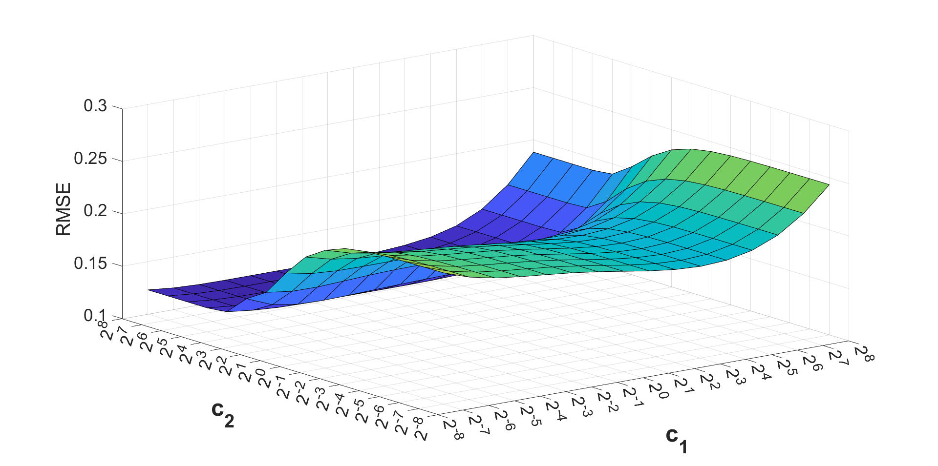
(a) qsar_aquatic toxicity

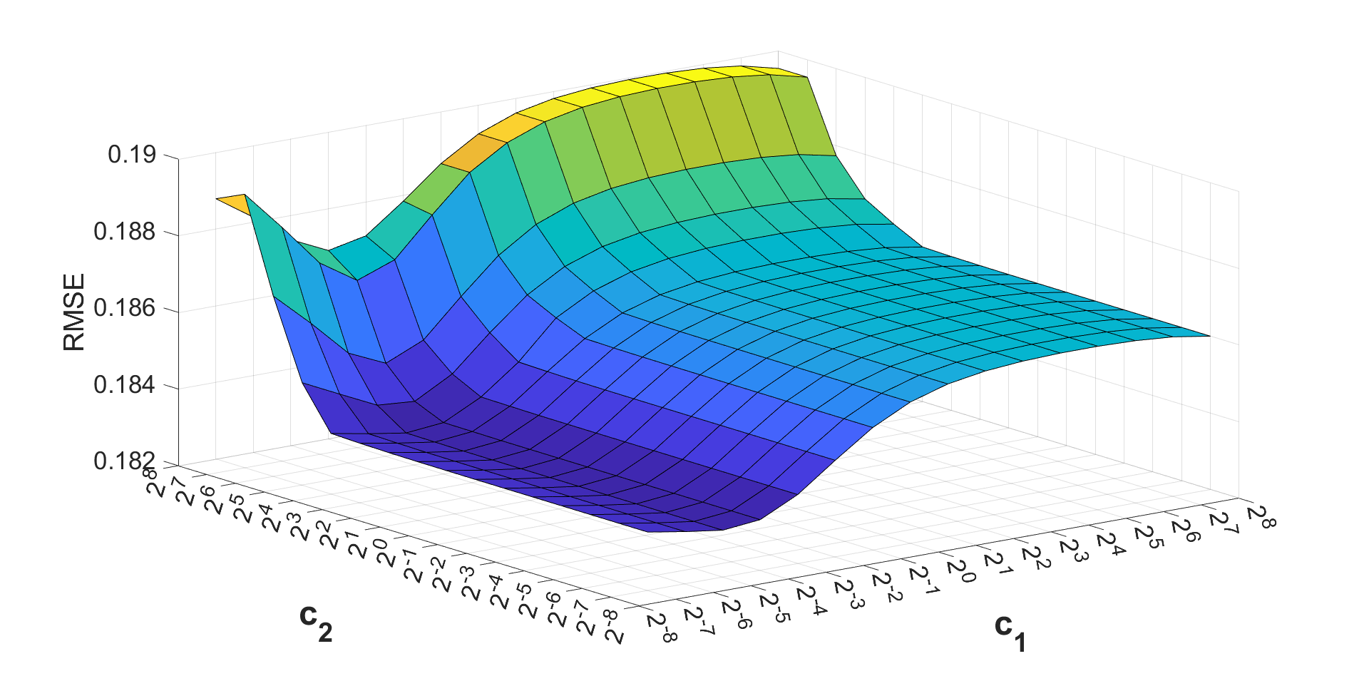
(b) servo

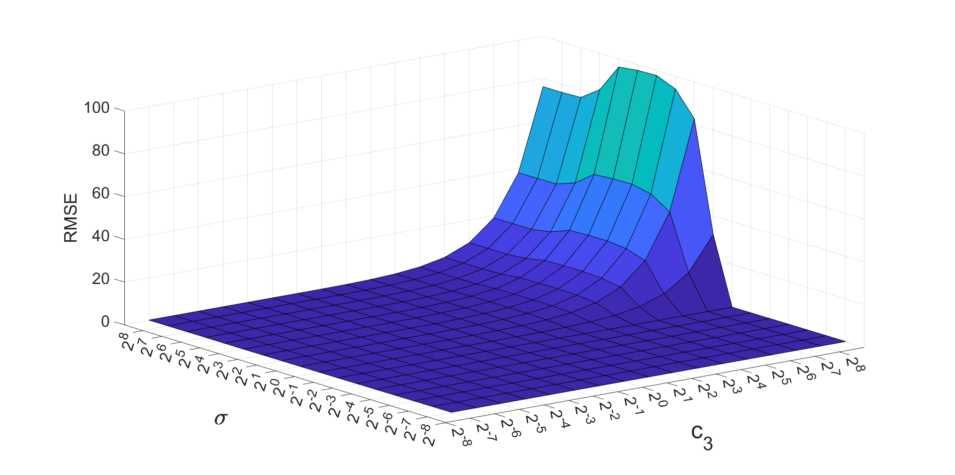
(c) Auto-price

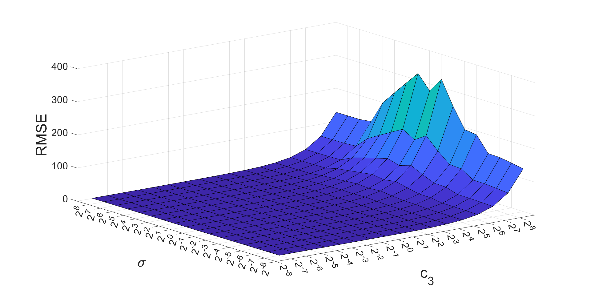
(d) gas_furnace2

Figure 1: Influence of parameters on the RMSE values of the proposed TSVR+.

Figures 1 show the dependence of the RMSE values of the proposed TSVR+ on the UCI datasets. Figure 1(a) and 1(b) denote the variation in RMSE values along with the hyperparameters $c_{1}$ and $c_{2}$. Other parameters are fixed at their optimal values. Figures 1(c) and 1(d) illustrate the dependence of RMSE of the proposed TSVR+ on the hyperparameters $c_{3}$ and kernel parameter $\sigma$. Hence, optimal RMSE values are highly dependent on the parameters.

4.4 Statistical analysis

In this subsection, we conduct a statistical assessment on the performance of the baseline models TSVR, $\epsilon$-TSVR, TWSVR, TSVQR and proposed TSVR+ by employing Friedman test and Nemenyi post hoc test [54]. The Friedman test statistically compares the models with the null hypothesis assumption that all models are equivalent and the Nemyeni test compares the models pairwise. Assuming $l$ and $n$ signify the number of models and number of datasets, respectively, the statistic is calculated using the relation:

$$\chi_{F}^{2}=\frac{12n}{l(l+1)}\Bigg{[}\sum_{i=1}^{l}r_{i}^{2}-\frac{l(l+1)^{2}}{4}\Bigg{]},$$

where $r_{i}$ signifies the average rank of $i^{th}$ model. $\chi_{F}^{2}$ has $(l-1)$ degree of freedom. The undesirable conservative nature of Friedman statistic can be overcome by F-distribution [54]. It has degree of freedom $((l-1),(l-1)(n-1))$ and is defined through the relation:

$$F_{F}=\frac{(n-1)\chi_{F}^{2}}{n(l-1)-\chi_{F}^{2}}.$$

We analyze the models in a pairwise way by using the Nemyeni test which concludes that the models are significantly different if the difference in their rank is greater than the critical difference (cd). It is calculated as

$$cd=q_{\alpha}\sqrt{\frac{l(l+1)}{6n}}.$$

First, we statistically analyse the artificially generated datasets for which we have $l=5$ and $n=9$. On calculating, we obtain $\chi_{F}^{2}=22.8838$ and $F_{F}=13.9575$ with degree of freedom $4$ and $(4,32)$, respectively. $F_{(4,32)}=2.6684$ $<$ $F_{F}$. Thus, the null hypothesis fails and the models are not equivalent. Further, we employ the Nemyeni test and calculate $cd=2.033$. We can observe from Table 2 that TWSVR and TSVQR are significantly different from the proposed TSVR+ as the difference in their ranks is greater than cd. Despite the rank difference of TSVR and $\epsilon$ TSVR, with the proposed TSVR+ being smaller than cd, results clearly demonstrate the superiority of the proposed TSVR+.

For the numerical experiments on UCI and stock datasets, we have $n=16$ and $l=5$. Thus degree of freedom of $\chi_{F}^{2}$ and $F_{F}$ are obtained as $4$ and $(4,60)$, respectively. At $5\%$ level of significance, $F_{(4,60)}=2.5252$. Using the average ranks of the model based on the RMSE values depicted in Table 5, we calculate

$$\chi_{F}^{2}=\frac{12\times 16}{5\times 6}\Bigg{[}3^{2}+3^{2}+3.18^{2}+3.88^{2}+1.94^{2}-\frac{5\times 6^{2}}{4}\Bigg{]}=12.3546$$

and

$$F_{F}=\frac{(16-1)\times 12.3546}{16\times 4-12.3546}=3.5883$$

which is greater than the $F_{(4,60)}$. Hence, the null hypothesis fails and the algorithms under comparison are not equivalent.

Similarly, the average ranks of the models with respect to the SSR/SST values are depicted in Table 7 using which we calculate $\chi_{F}^{2}=9.7786$ and $F_{F}=2.7051$ which is greater than $F_{(4,60)}=2.5252$. Therefore, the null hypothesis is rejected which leads to the non-equivalence of the models. For the metric SSE/SST, using the average rank mentioned in Table 6, we get the calculated $\chi_{F}^{2}=5.2064$ and $F_{F}=1.3283$. Though the $F_{F}$ value, in this case, is less than $F_{(4,60)}=2.5252$, other cases clearly show the baseline models and the proposed TSVR+ are not equivalent.

5 Application

In this section, we apply the proposed TSVR+ and the existing TSVR [13] on the time series real-world datasets [55] to demonstrate the application of the proposed TSVR+ model. In order to consider the impact of PI on the TSVR model, we compared the proposed model with TSVR, only. We conducted random $70:30$ splitting for training and testing, respectively, and the ranges of different parameters considered are consistent with synthetic datasets. The datasets are normalized using min-max normalization (equation 35). Table 8 represents the performance of the models on the time series dataset along with the details of the datasets. The proposed TSVR+ has least RMSE value for the NNGC1_dataset_D1_V1_004, NNGC1_dataset_D1_V1_006, NNGC1_dataset_D1_V1_007, NNGC1_dataset_D1_V1_009, NNGC1_dataset_D1_V1_010, NNGC1_dataset_E1_V1_001, NNGC1_dataset_E1_V1_008, NNGC1_dataset_E1_V1_009 having values 0.15498, 0.08495, 0.12537, 0.13483, 0.14758, 0.19482, 0.11658 and, 0.11513 respectively. The average RMSE value of TSVR and proposed TSVR+ are $0.14117$ and $0.13627$, respectively. Thus, the RMSE, SSE/SST and SSR/SST values clearly reflect the better performance of the proposed TSVR+ in comparison to TSVR.

Table 8: RMSE values along with SSE/SST and SSR/SST on the time series datasets for TSVR and the proposed TSVR+. The best values are highlighted in bold.

Dataset	Metric	TSVR [13]	proposed TSVR+
(#samples,#features)
NNGC1_dataset_D1_V1_003	RMSE	0.15153	$0.15219$
$(430,5)$	SSE/SST	0.71002	$0.72376$
	SSR/SST	$0.3287$	0.4051
NNGC1_dataset_D1_V1_004	RMSE	$0.15573$	0.15498
$(545,5)$	SSE/SST	$0.78086$	0.77665
	SSR/SST	$0.19448$	0.19567
NNGC1_dataset_D1_V1_006	RMSE	$0.08586$	0.08495
$(610,5)$	SSE/SST	$0.20293$	0.1986
	SSR/SST	0.75693	$0.72234$
NNGC1_dataset_D1_V1_007	RMSE	$0.12554$	0.12537
$(610,5)$	SSE/SST	$0.60823$	0.60773
	SSR/SST	$0.33857$	0.34223
NNGC1_dataset_D1_V1_009	RMSE	$0.13802$	0.13483
$(540,5)$	SSE/SST	$0.64329$	0.615
	SSR/SST	$0.60259$	0.60309
NNGC1_dataset_D1_V1_010	RMSE	$0.15069$	0.14758
$(585,5)$	SSE/SST	$0.67146$	0.66717
	SSR/SST	$0.19536$	0.20483
NNGC1_dataset_E1_V1_001	RMSE	$0.21357$	0.19482
$(370,5)$	SSE/SST	$0.6437$	0.5343
	SSR/SST	0.44724	$0.36654$
NNGC1_dataset_E1_V1_008	RMSE	$0.1261$	0.11658
$(740,5)$	SSE/SST	$0.83933$	0.71866
	SSR/SST	0.94612	$0.56703$
NNGC1_dataset_E1_V1_009	RMSE	$0.12352$	0.11513
$(740,5)$	SSE/SST	$0.86062$	0.74768
	SSR/SST	0.84118	$0.64843$
Average RMSE		0.14117	0.13627

6 Conclusion

In the process of human learning, along with the main topic, teachers often enhance understanding of students by providing additional information, such as various examples, counterexamples, and explanatory comments. Twin support vector regression (TSVR) is an efficient regression model which gets trained solely on normal features, lacking the benefit of additional context or information that may further enhance its learning capabilities. This paper introduced the fusion of learning using privileged information (LUPI) with the TSVR and proposed a novel twin support vector regression using privileged information proposed (TSVR+). It effectively combined the original features with the privileged knowledge to improve the generalization performance. The proposed TSVR+ considers the structural risk minimization principle by incorporating regularization terms corresponding to the regressor function as well as the correction function, thus preventing overfitting. In order to train the proposed model efficiently, we choose the successive overrelaxation technique. To assess the superiority of models, we conducted numerical experiments on the UCI, stock and time series datasets. The numerical results and its statistical analysis demonstrate the superiority of the proposed model. However, it’s worth noting that the proposed model has a limitation of high time consumption for parameter tuning. This limitation can be overcome by incorporating different efficient tuning techniques to streamline the tuning process and improve overall efficiency.

References

- Vapnik [1999] Vladimir N Vapnik. An overview of statistical learning theory. IEEE Transactions on Neural Networks, 10(5):988–999, 1999.
- Deylami and Singh [2012] Hanif-Mohaddes Deylami and Yashwant Prasad Singh. Adaboost and SVM based cybercrime detection and prevention model. Artif. Intell. Res., 1(2):117–130, 2012.
- Chen et al. [2015] Chuanfa Chen, Yanyan Li, Changqing Yan, Honglei Dai, and Guolin Liu. A robust algorithm of multiquadric method based on an improved huber loss function for interpolating remote-sensing-derived elevation data sets. Remote Sensing, 7(3):3347–3371, 2015.
- Liu et al. [2018] Lingling Liu, Yuejin Zhao, Lingqin Kong, Ming Liu, Liquan Dong, Feilong Ma, and Zongguang Pang. Robust real-time heart rate prediction for multiple subjects from facial video using compressive tracking and support vector machine. Journal of Medical Imaging, 5(2):024503–024503, 2018.
- Hazarika et al. [2020] Barenya Bikash Hazarika, Deepak Gupta, and Mohanadhas Berlin. Modeling suspended sediment load in a river using extreme learning machine and twin support vector regression with wavelet conjunction. Environmental Earth Sciences, 79:1–15, 2020.
- Smola and Schölkopf [2004] Alex J Smola and Bernhard Schölkopf. A tutorial on support vector regression. Statistics and Computing, 14:199–222, 2004.
- Drucker et al. [1996] Harris Drucker, Christopher J Burges, Linda Kaufman, Alex Smola, and Vladimir Vapnik. Support vector regression machines. Advances in Neural Information Processing Systems, 9, 1996.
- Pani and Mohanta [2014] Ajaya Kumar Pani and Hare Krishna Mohanta. Soft sensing of particle size in a grinding process: Application of support vector regression, fuzzy inference and adaptive neuro fuzzy inference techniques for online monitoring of cement fineness. Powder Technology, 264:484–497, 2014.
- Wu et al. [2004] Chun-Hsin Wu, Jan-Ming Ho, and Der-Tsai Lee. Travel-time prediction with support vector regression. IEEE Transactions on Intelligent Transportation Systems, 5(4):276–281, 2004.
- Wu et al. [2007] Zhi-li Wu, Chun-hung Li, Joseph Kee-Yin Ng, and Karl RPH Leung. Location estimation via support vector regression. IEEE Transactions on Mobile Computing, 6(3):311–321, 2007.
- Jayadeva et al. [2007] Jayadeva, Reshma Khemchandani, and Suresh Chandra. Twin support vector machines for pattern classification. IEEE Transactions on Pattern Analysis and Machine Intelligence, 29(5):905–910, 2007.
- Tanveer et al. [2022] Mohammad Tanveer, T Rajani, Reshma Rastogi, Yuan-Hai Shao, and MA Ganaie. Comprehensive review on twin support vector machines. Annals of Operations Research, pages 1–46, 2022.
- Peng [2010] Xinjun Peng. TSVR: an efficient twin support vector machine for regression. Neural Networks, 23(3):365–372, 2010.
- Shao et al. [2013] Yuan-Hai Shao, Chun-Hua Zhang, Zhi-Min Yang, Ling Jing, and Nai-Yang Deng. An -twin support vector machine for regression. Neural Computing and Applications, 23:175–185, 2013.
- Xu and Wang [2012] Yitian Xu and Laisheng Wang. A weighted twin support vector regression. Knowledge-Based Systems, 33:92–101, 2012.
- Zhao et al. [2013] Yong-Ping Zhao, Jing Zhao, and Min Zhao. Twin least squares support vector regression. Neurocomputing, 118:225–236, 2013.
- Peng et al. [2014] Xinjun Peng, Dong Xu, and Jindong Shen. A twin projection support vector machine for data regression. Neurocomputing, 138:131–141, 2014.
- Bi and Bennett [2003] Jinbo Bi and Kristin P Bennett. A geometric approach to support vector regression. Neurocomputing, 55(1-2):79–108, 2003.
- Khemchandani et al. [2016] Reshma Khemchandani, Keshav Goyal, and Suresh Chandra. TWSVR: regression via twin support vector machine. Neural Networks, 74:14–21, 2016.
- Huang et al. [2022] Huajuan Huang, Xiuxi Wei, and Yongquan Zhou. An overview on twin support vector regression. Neurocomputing, 490:80–92, 2022.
- Shi and Chen [2023] Ting Shi and Sugen Chen. Robust twin support vector regression with smooth truncated H loss function. Neural Processing Letters, pages 1–45, 2023.
- Anagha et al. [2018] P Anagha, S Balasundaram, and Yogendra Meena. On robust twin support vector regression in primal using squared pinball loss. Journal of Intelligent & Fuzzy Systems, 35(5):5231–5239, 2018.
- Gupta and Gupta [2021a] Deepak Gupta and Umesh Gupta. On robust asymmetric lagrangian -twin support vector regression using pinball loss function. Applied Soft Computing, 102:107099, 2021a.
- Liu et al. [2021] Ming-Zeng Liu, Yuan-Hai Shao, Chun-Na Li, and Wei-Jie Chen. Smooth pinball loss nonparallel support vector machine for robust classification. Applied Soft Computing, 98:106840, 2021.
- Niu et al. [2017] Jiayi Niu, Jing Chen, and Yitian Xu. Twin support vector regression with huber loss. Journal of Intelligent & Fuzzy Systems, 32(6):4247–4258, 2017.
- Balasundaram and Prasad [2020] S Balasundaram and Subhash Chandra Prasad. Robust twin support vector regression based on huber loss function. Neural Computing and Applications, 32:11285–11309, 2020.
- Gupta and Gupta [2021b] Umesh Gupta and Deepak Gupta. On regularization based twin support vector regression with huber loss. Neural Processing Letters, 53(1):459–515, 2021b.
- Ye et al. [2023] Yafen Ye, Zhihu Xu, Jinhua Zhang, Weijie Chen, and Yuanhai Shao. Twin support vector quantile regression. arXiv preprint arXiv:2305.03894, 2023.
- Hazarika et al. [2022] Barenya Bikash Hazarika, Deepak Gupta, and Narayanan Natarajan. Wavelet kernel least square twin support vector regression for wind speed prediction. Environmental Science and Pollution Research, 29(57):86320–86336, 2022.
- Ganaie et al. [2022a] MA Ganaie, M Tanveer, and Iman Beheshti. Brain age prediction using improved twin SVR. Neural Computing and Applications, pages 1–11, 2022a.
- Ganaie et al. [2022b] MA Ganaie, M Tanveer, and Iman Beheshti. Brain age prediction with improved least squares twin SVR. IEEE Journal of Biomedical and Health Informatics, 27(4):1661–1669, 2022b.
- Nidhi and Lobiyal [2022] Nidhi Nidhi and DK Lobiyal. Traffic flow prediction using support vector regression. International Journal of Information Technology, 14(2):619–626, 2022.
- Vapnik and Vashist [2009] Vladimir Vapnik and Akshay Vashist. A new learning paradigm: Learning using privileged information. Neural Networks, 22(5-6):544–557, 2009.
- Feyereisl and Aickelin [2012] Jan Feyereisl and Uwe Aickelin. Privileged information for data clustering. Information Sciences, 194:4–23, 2012.
- Motiian et al. [2016] Saeid Motiian, Marco Piccirilli, Donald A Adjeroh, and Gianfranco Doretto. Information bottleneck learning using privileged information for visual recognition. In Proceedings of the IEEE Conference on Computer Vision and Pattern Recognition, pages 1496–1505, 2016.
- Tang et al. [2019] Jingjing Tang, Yingjie Tian, Dalian Liu, and Gang Kou. Coupling privileged kernel method for multi-view learning. Information Sciences, 481:110–127, 2019.
- Xu et al. [2015] Xinxing Xu, Wen Li, and Dong Xu. Distance metric learning using privileged information for face verification and person re-identification. IEEE Transactions on Neural Networks and Learning Systems, 26(12):3150–3162, 2015.
- Yang et al. [2017] Xun Yang, Meng Wang, and Dacheng Tao. Person re-identification with metric learning using privileged information. IEEE Transactions on Image Processing, 27(2):791–805, 2017.
- Niu and Wu [2012] Lingfeng Niu and Jianmin Wu. Nonlinear support vector machines for learning using privileged information. In 2012 IEEE 12th International Conference on Data Mining Workshops, pages 495–499. IEEE, 2012.
- Li et al. [2018] Xue Li, Bo Du, Chang Xu, Yipeng Zhang, Lefei Zhang, and Dacheng Tao. R-SVM+: Robust learning with privileged information. In IJCAI, pages 2411–2417, 2018.
- Che et al. [2021] Zhiyong Che, Bo Liu, Yanshan Xiao, and Hao Cai. Twin support vector machines with privileged information. Information Sciences, 573:141–153, 2021.
- Gautam et al. [2017] Chandan Gautam, Aruna Tiwari, and Qian Leng. On the construction of extreme learning machine for online and offline one-class classification—an expanded toolbox. Neurocomputing, 261:126–143, 2017.
- Vovk [2013] Vladimir Vovk. Kernel ridge regression. In Empirical Inference: Festschrift in Honor of Vladimir N. Vapnik, pages 105–116. Springer, 2013.
- Malik et al. [2023] Ashwani Kumar Malik, Ruobin Gao, MA Ganaie, Muhammad Tanveer, and Ponnuthurai Nagaratnam Suganthan. Random vector functional link network: recent developments, applications, and future directions. Applied Soft Computing, page 110377, 2023.
- Gautam et al. [2020] Chandan Gautam, Aruna Tiwari, and Muhammad Tanveer. AEKOC+: Kernel ridge regression-based auto-encoder for one-class classification using privileged information. Cognitive Computation, 12:412–425, 2020.
- Gautam et al. [2019] Chandan Gautam, Aruna Tiwari, and Muhammad Tanveer. KOC+: Kernel ridge regression based one-class classification using privileged information. Information Sciences, 504:324–333, 2019.
- Zhang and Yang [2020] Peng-Bo Zhang and Zhi-Xin Yang. A new learning paradigm for random vector functional-link network: RVFL+. Neural Networks, 122:94–105, 2020.
- Mangasarian and Musicant [1999] Olvi L Mangasarian and David R Musicant. Successive overrelaxation for support vector machines. IEEE Transactions on Neural Networks, 10(5):1032–1037, 1999.
- Luo and Tseng [1993] Zhi-Quan Luo and Paul Tseng. Error bounds and convergence analysis of feasible descent methods: a general approach. Annals of Operations Research, 46(1):157–178, 1993.
- Burges and Crisp [1999] Christopher J Burges and David Crisp. Uniqueness of the svm solution. Advances in Neural Information Processing Systems, 12, 1999.
- Dua and Graff [2017] Dheeru Dua and Casey Graff. UCI machine learning repository. 2017.
- Tanveer and Shubham [2017] Muhammad Tanveer and K Shubham. A regularization on lagrangian twin support vector regression. International Journal of Machine Learning and Cybernetics, 8(3):807–821, 2017.
- Tanveer et al. [2016] Muhammad Tanveer, K Shubham, Mujahed Aldhaifallah, and Shen-Shyang Ho. An efficient regularized k-nearest neighbor based weighted twin support vector regression. Knowledge-Based Systems, 94:70–87, 2016.
- Demšar [2006] Janez Demšar. Statistical comparisons of classifiers over multiple data sets. The Journal of Machine Learning Research, 7:1–30, 2006.
- Derrac et al. [2015] J Derrac, S Garcia, L Sanchez, and F Herrera. KEEL data-mining software tool: Data set repository, integration of algorithms and experimental analysis framework. J. Mult. Valued Log. Soft Comput, 17:255–287, 2015.