Lower-bounding entanglement with nonlocality in a general Bell’s scenario
Abstract
Understanding the quantitative relation between entanglement and Bell nonlocality is a long-standing open problem of both fundamental and practical interest. Here we provide a general approach to address this issue. Starting with an observation that entanglement measures, while defined dramatically different in mathematics, are basically the distances between the state of interest and its closest separable state, we relate this minimal distance between states with distance-based Bell nonlocality, namely, the minimal distance between correlation of interest with respect to the set of classical correlations. This establishes the quantitative relation between entanglement and Bell nonlocality, leading to the bounds for entanglement in various contexts. Our approach enjoys the merits of: (i) generality, it applies to any Bell’s scenario without requiring the information of devices and to many entanglement measures, (ii) faithfulness, it gives a non-trivial entanglement estimation from any nonlocal correlation.
pacs:
03.65.Ta, 03.65.UdStrongly correlated quantum subsystems could be entangled and behave like a single physical subject. That is, a local measurement on one subsystem can instantaneously modifies the states of other subsystems even if they are in a space-like distance [1]. By choosing the measurement settings for each subsystem properly, one could obtain correlations between outcomes going beyond the scope allowed by the classical tenets of realism and locality. This can be verified by the violation of Bell’s inequality, referred to as nonlocality [2]. Entanglement and nonlocality draw clear cut between quantum theory and classical ones [3, 4, 5, 2, 1]. Practically, they are also appreciated as the key resources for quantum advantages in many information tasks, such as, quantum teleportation [6], quantum cryptography [7], quantum algorithms [8, 9, 10], and quantum metrology [11]. Motivated by the fundamental interest and also practical usage like device-independent (DI) estimation of entanglement (where no information about devices are used thus robust to all the systematic errors) [12], the interplay between entanglement and nonlocality has been exploited intensely [13, 14, 15, 16, 17, 18, 19, 20, 21].
It is clear that entanglement is necessary for ¡¡ nonlocality, however, establishing quantitative relation between them encounters inevitable difficulties. On the one hand, entanglement and nonlocality are distinct concepts, and their interrelation turns out to be quite subtle: (1) there are entangled states that do not demonstrate nonlocality [22] and (2) maximum ¡¡ nonlocality does not always call for the maximum entanglement [23]. On the other hand, in the theory of entanglement, entanglement measures are defined dramatically different in mathematics. For most of them, analytical computation is even NP-hard [24, 25, 26]. Only in some special cases, such as two-qubit systems, the computation can be thoroughly done [1]. These specific analytical results become the key ingredients to estimate entanglement in the relevant minimal Bell’s scenario [27, 28]. In general, such useful results are missing. Till now, except the entanglement measure of negativity [12], it is still an open question that how to establish quantitative connections between entanglement measures, especially the ones having clear operational meanings, and nonlocality in general Bell’s scenarios.
To answer this question, we provide a general framework enabling one to estimate various measures of entanglement while not requiring background knowledge about quantum systems or Bell’s scenario. Our starting point is that, though entanglement measures may have drastically different forms, they are all related to the minimal distance of the concerned state with respect to the set of separable states. Similarly, nonlocality is also quantified by the distance between the correlation of interest to the closest local correlation. Inspired by this similarity, we connect these two distances and provide nontrivial lower bounds for entanglement measures with any nonlocal correlation. Especially, we can estimate the extremely weak form of entanglement, namely, bound entanglement. Our estimation can be asymptotically tight in some multipartite systems.
I Results
Lower bounding Entanglement with distance with respect to closest separable state.—The most intuitive method to quantify entanglement is the minimal distance of a concerned state with respect to the set of the separable states [29, 30], that is,
| (1) |
where is a distance measure of states. Clearly, different choices of state distances give rise to different entanglement measures [31, 30, 32, 33]. For example, choosing the relative entropy as the distance measure , one obtains the relative entropy of entanglement [30], which serves as an upper bound for the entanglement of distillation [34]. With the trace-distance where , which quantifies how well two states can be operationally distinguished [35], one can define a measure as the distinguishability of the state from the set of separable states.
Another relevant method is the convex-roof construction [36]: Starting with a measure established for a pure state , denoted as , then it can be extended to a general mixed state via the convex-roof construction as , where the minimization is taken over all possible decompositions . The entanglement of formation [37], the concurrence , and the geometric measure of entanglement [38, 39] are defined in this way. Besides the aforementioned two major approaches, there are also other measures such as the robustness of entanglement to noise [39]. We recall the corresponding definitions in Methods.
Our first key observation is: besides measures and that are directly defined in terms of minimal state distances, the other measures relate also closely to the minimal distance (see Methods for the proof):
| (2) | ||||
where fidelity and infidelity . For pure states, these lower bounds are tight for the first three measures.
Relation between entanglement and Bell nonlocality.— Let us first recall a general Bell scenario: space-like separated observers, share a joint -partite system. Each observer, e.g., , can randomly perform one measurement from the set of all possible ones and obtains an outcome . By we specify the joint probability of obtaining outcomes under the measurement settings . The collection of such probabilities , with over measurement settings and outcomes, is referred to as a behavior [40]. If a behavior allows a quantum realization, there exists at least one state and a set of measurements such that the behavior with specifying the measurement operator corresponding to the outcome under the setting on ’s side.
Classical physics assumes realism and locality, and one observable’s value is determined before the implementation of the measurement by hidden variables. Thus the set of local behaviors, specified by , is a convex polytope with the vertices to be the extreme deterministic behaviors and the facets being tight Bell inequalities [2]:
| (3) |
where specifies the maximum classical value of Bell’s quantity. A violation of a given Bell inequality, namely, , certifies nonlocality, and the degree is taken as a natural quantification of nonlocality. However, such a quantification highly depends on the Bell’s inequality involved, and a nonlocal behavior may not violate an unsuitably chosen Bell’s inequalities and thus it cannot be verified. Alternatively, noting that one behavior is non-local if and only if it is not in the polytope formed by classical correlations, one can consider the minimal distance between the concerned behavior with respect to classical ones as
| (4) |
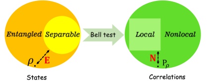
where is a classical distance measure between distributions and and with we specify the number of different choices of measurement settings . This minimum distance [41], capturing how a concerned behavior goes beyond the local ones, quantifies nonlocality in a different way from the Bell’s violation and is referred to as distance-based Bell nonlocality here. As the set of local correlations can be well characterized in principle for any given Bell scenario [42, 2], for a given behavior we can compute the distance by an optimization over the set of local behaviors. In what follows, we show such distance-based quantifications of entanglement and nonlocality can be unified, for which, a geometrical illustration is shown in Fig.1.
As far as local measurements of settings performed on and are concerned, it follows from data processing inequality that
| (5) |
where specifies the statistics distance induced by state distance . For example, the statistics distance arising from the trace-distance is the Kolmogorov distance . Denote the closest separable state to the state , then is the distance-based entanglement defined via Eq.(1). As there are different choices of in Eq.(5), each of them relates to an inequality of the form Eq.(5). As implies the corresponding behavior , summing Eq.(5) over all possible ’s we have
| (6) |
To this end, we have bounded the distance of state away from the set of separable states by statistics in a general Bell’s scenario. Combined with our observation Eq.(2), we then have
Theorem.1 (Lower-bounding entanglement with distance-based nonlocality) Entanglement measures have lower bounds in terms of functions of distance-based nonlocality as
| (7) | ||||
This provides an answer for the long-standing open question how entanglement relates to nonlocality, allowing one to estimate various entanglement measures in DI setting.
We also note that the distance-based nonlocality is not easy to compute in a multipartite scenario. This is because there are exponentially increasing deterministic extreme correlations with respect to the size of system [43, 44, 45, 46], rendering the typical linear programming approach for characterization the set inefficient [47]. To overcome this difficulty, we also provide an estimation solely with the Bell’s violation. We first lower-bound with violation of Bell’s inequality (see Methods)
| (8) |
where . Second, by lower-bounding those entanglement measures with (see Methods), we finally obtain their lower bounds in terms of Bell violations
Theorem.2 (Lower-bounding entanglement with Bell’s violation)With the degree of modified Bell’s violation , we have lower bounds on entanglement measures as
| (9) |
Examples.— In the following, we illustrate our results with several examples. First, let us consider the minimal Bell scenario, where there are two parties, and in every round they each can locally perform one of the two binary measurements indexed by where the outcomes are labeled by . In this setting, the facets of the classical correlation polytope is given by one Bell’s inequality up to the relabelling of measurements and outcomes, namely, the Clauser-Horne-Shimony-Holt (CHSH) inequality [48]
| (10) |
In this scenario, the quantity has been already quantitatively related to and [27, 28, 49], where the thorough study of entanglement for two-qubit system has lots implications, including the computation of entanglement measures, the quantitative connection between concurrence and Bell’s violation as [28] in two-qubit system, and also Jordan’s lemma [50, 51, 52] which extends this connection to an arbitrary dimensional system. Here, following this line of research, the estimation that can also be given (See Methods).
Our framework, namely, Theorems 1 and 2, provides a sub-optimal bound without using the relevant results of entanglement and nonlocality. For example, consider the behavior which maximally violates CHSH inequality. Interestingly, by exploiting symmetry we can give the classical correlation closest to the behavior as (Methods). We have then the lower bounds following Theorem 1: , , . By making use of Theorem 2, we obtain , , , where these lower bounds are smaller due to the fact that Theorem 2 is a relaxation of Theorem 1. Our lower bounds can be tighten when more details of the scenario are considered. Notice that a maximal CHSH violation is well-known to self-test anti-communting qubit measurements for both Alice and Bob [53, 54]. For such measurements, the maximum value of Bell’s function for separable states is (see Methods), namely, for . Therefore, one can replace the with . Then we have , , , and .
We also note that our lower-bound could be already tight for some Bell’s scenarios. Let us consider the Bell’s scenario, namely, parties, two measurements per party and two outcomes per measurement. When the total number of parties is odd, the Mermin-Ardehali-Belinskii-Klyshko (MABK) inequality [43, 55, 56, 57] can be cast into (see Methods)
| (11) |
where with specifying the setting on -th observer and . The maximal violation of the MABK inequality is achieved by -partite GHZ state and for each observer the settings are chosen as . In this case, with classical bound and the maximal quantum violation , the DI lower bound reads
which tends to the exact value of trace-distance measure of entanglement of -partite GHZ state in the case of infinite . In all the examples above, the estimation for other relevant entanglement measures, e.g., , , and can be obtained similarly via Theorem 2.
As the second example, we consider a bipartite scenario and show that bound entanglement, albeit very weak and can not be detected by negativity [12], still allows for a DI quantification with our approach. Let us consider a scenario due to Yu and Oh, in which, the party Alice performs dichotomic measurements labeled with while another party Bob performs only two measurements with the first one, labeled with 0, being dichotomic and the second one, labeled with 1, having outcomes. For any local realistic model, it holds [58]
| (12) |
It is clear that the total number of possible measurement settings and a violation to this inequality will lead to a nontrivial estimation of as
| (13) |
which provide DI estimation of entanglement for a family of nonlocal bound entangled states [58].
Conclusion and discussion.— Understanding the quantitative connection between entanglement and Bell nonlocality is a fundamental issue. Previously, this connection is considered mainly in the minimal Bell’s scenario, but remained almost unexplored in general Bell’s scenarios where the structures of relevant entanglement and nonlocality are not well-understood. Here, we exploit the basic idea in quantifying these two quantities. We also find that although entanglement measures are defined with different strategies, they closely relate to the distances between state of interest with respect to the set of separable states. We then show that this kind of state distance can be estimated in Bell’s scenarios with the distance between the relevant correlation to the closest classical correlations. Thus, we obtained a feasible and versatile approach to estimate many entanglement measures, including the entanglement of formation, the robustness of entanglement, the entanglement of concurrence, and the geometric measure of entanglement. Especially, we did not assume anything on the functionalities of devices, which means one can estimate entanglement experimentally in a device-independent manner, which is robust to any kind of systematic noise.
The quantitative relation between entanglement and Bell nonlocality established here upgrades the claim that Bell nonlocality verifies entanglement into Bell nonlocality lower bounds entanglement, although the lower bounds sometimes are not tight. For further research, we believe our framework may immediately applies to the issue of, for example, quantitatively study of the rich structure of multipartite entanglement, especially the quantification of genuinely multipartite entanglement.
Acknowledgements.
L.L.S. and S.Y. would like to thank Key-Area Research and Development Program of Guangdong Province Grant No. 2020B0303010001. Z.P.X. acknowledges support from National Natural Science Foundation of China (Grant No. 12305007), Anhui Provincial Natural Science Foundation (Grant No. 2308085QA29).II Methods.
Entanglement of formation and the relative entropy of entanglement.— Entanglement of formation [37] is defined via a convex-roof construction with the pure state measure defined as the von Neumann entropy of subsystem where , which is equivalent to the minimal distance of to set of separable state, namely, [1]. Denoting the ensemble and the closest separable state of as , we have
where and the second inequality is due to the convexity of relative entropy. It follows the quantum Pinsker inequality that
where specifies the closest separable state of with respective to the relative entropy.
Concurrence — Entanglement concurrence is defined via convex-roof construction with the pure state measure with specifying the diagonal parts in Schmidt basis, where is fidelity. Specify the decomposition achieving the convex-roof with and the closest separable state for as with respect to the measure of infidelity, we then has
| (14) | |||||
where . We have , we have used the inequality . Then it follows
| (15) | |||||
Geometric measure of entanglement.— The geometric measure of entanglement [38, 39] is a convex-roof of , i.e., via the maximal squared overlap with the separable pure states. We note that . Specify ensemble achieving the convex-roof as the closest pure separable state to as . We note ,
| (16) | |||||
| (17) |
where , and we have used the joint-convexity of infidelity in the second inequality. For arbitrary two pure states , we have . Then, we have
Robustness of Entanglement.— There are also other measures such as the robustness of entanglement [39]
| (18) |
where is the minimal number for some separable state such that the mixture becomes separable. This measure quantifies the robustness of entanglement to noise. For the , we specify the the optimal separable state as and minimal wight as , then . From it follows We thus arrive at
| (19) |
Lower bound in minimal Bell’s scenario.— We recall that, for two binary measurements, say and , acting in Hilbert space of finite dimension. There are decompositions and , such that are two-dimensional and are projective measurements acting on it. This argument applies to the measurements on Bob’s side. With notions and specifying the projectors on the space and and , . It follows the monotonicity of entanglement measure under physical operation that
Note that, any two-qubit state can be convert into the one diagonal in Bell’s basis [52] via local operation and classical communication while not changing the maximum score of Bell’s inequaity. We specify such diagonal state corresponding to by . Definitely, . Then we have
| (20) |
For Bell’s diagonal state, one has , via a the technique like convex closure to acquire a closed form, one has [49]
| (21) | |||||
Focus on , for two-qubit system one has [39], thus we have
| (22) | |||||
Optimizing the estimation of entanglement with the maximum Bell nonlocality of CHSH inequality. — When the maximum value of CHSH inequality is , the measurements on each side are self-test to be mutually unbiased. For them, there are well-known uncertainty relations and . These relations imply a bound on . Specifically, for a product state , one has the correlations as and . The uncertainty relations then imply . Then one can optimizing the distance within the correlation .
Proof of Theorem 2 — Given an arbitrary Bell inequality
and denote
we have
where with is the nearest separable state for under trance distance and
Symmetry — The CHSH inequality is maximally violated by the correlation where
This correlation is highly symmetric, e.g., it is unchanged under the following transformations
-
i)
and ;
-
ii)
and and
for arbitrary , where addition is modular 2. Next we shall show that i) the nearest local correlation shares the same symmetry and ii) this symmetry determines the local correlation to be of form
with in order to satisfy the CHSH inequality. For a local correlation we denote
so that
In order to evaluate
we note that
Thus a new correlation
is not farer away from , where
In the similar manner from symmetry ii it follows that the new correlation
with . To satisfy CHSH inequality it is clear that so that we obtain
Proof of Eq.(11) — In a local realistic model, we have
and we shall prove by induction on odd that
where we have denoted with and average is taken over . In fact, by noting that if we write it holds
and thus we have
from which it follows
Actually the upper bound for quantum theory is the algebraic upper bound for this inequality and is achieved by GHZ state. To show this we shall employ the graph state representation of GHZ state by complete graph
with stabilizers with and . By measuring observables for each party we obtain correlation
| (23) |
as a result of identity
References
- Horodecki et al. [2009] R. Horodecki, P. Horodecki, M. Horodecki, and K. Horodecki, Rev. Mod. Phys. 81, 865 (2009).
- Brunner et al. [2014] N. Brunner, D. Cavalcanti, S. Pironio, V. Scarani, and S. Wehner, Rev. Mod. Phys. 86, 419 (2014).
- Einstein et al. [1935] A. Einstein, B. Podolsky, and N. Rosen, Phys. Rev. 47, 777 (1935).
- Schödinger [1935] E. Schödinger, Math. Proc. Cambridge Philos. Soc. 31, 555 (1935).
- Bell [1964] J. S. Bell, Physics Physique Fizika 1, 195 (1964).
- Bennett et al. [1993] C. H. Bennett, G. Brassard, C. Crépeau, R. Jozsa, A. Peres, and W. K. Wootters, Phys. Rev. Lett. 70, 1895 (1993).
- Ekert [1991] A. K. Ekert, Phys. Rev. Lett. 67, 661 (1991).
- Raussendorf and Briegel [2001] R. Raussendorf and H. J. Briegel, Phys. Rev. Lett. 86, 5188 (2001).
- Raussendorf et al. [2003] R. Raussendorf, D. E. Browne, and H. J. Briegel, Phys. Rev. A 68, 022312 (2003).
- Briegel et al. [2009] H. J. Briegel, D. E. Browne, W. Dür, R. Raussendorf, and M. V. den Nest, Nat. Phys 5, 19 (2009).
- Giovannetti et al. [2004] V. Giovannetti, S. Lloyd, and L. Maccone, Science 306, 1330 (2004).
- Moroder et al. [2013] T. Moroder, J.-D. Bancal, Y.-C. Liang, M. Hofmann, and O. Gühne, Phys. Rev. Lett. 111, 030501 (2013).
- Yu et al. [2012] S. Yu, Q. Chen, C. Zhang, C. H. Lai, and C. H. Oh, Phys. Rev. Lett. 109, 120402 (2012).
- Yu et al. [2003] S. Yu, Z.-B. Chen, J.-W. Pan, and Y.-D. Zhang, Phys. Rev. Lett. 90, 080401 (2003).
- Acín et al. [2012] A. Acín, S. Massar, and S. Pironio, Phys. Rev. Lett. 108, 100402 (2012).
- Augusiak et al. [2015] R. Augusiak, M. Demianowicz, J. Tura, and A. Acín, Phys. Rev. Lett. 115, 030404 (2015).
- Masanes et al. [2008] L. Masanes, Y.-C. Liang, and A. C. Doherty, Phys. Rev. Lett. 100, 090403 (2008).
- Wiseman et al. [2007] H. M. Wiseman, S. J. Jones, and A. C. Doherty, Phys. Rev. Lett. 98, 140402 (2007).
- Barrett [2002] J. Barrett, Phys. Rev. A 65, 042302 (2002).
- Popescu [1995] S. Popescu, Phys. Rev. Lett. 74, 2619 (1995).
- Hardy [1993] L. Hardy, Phys. Rev. Lett. 71, 1665 (1993).
- Werner [1989] R. F. Werner, Phys. Rev. A 40, 4277 (1989).
- Acín et al. [2005] A. Acín, R. Gill, and N. Gisin, Phys. Rev. Lett. 95, 210402 (2005).
- Hill and Wootters [1997] S. Hill and W. K. Wootters, Phys. Rev. Lett. 78, 5022 (1997).
- Wootters [1998] W. K. Wootters, Phys. Rev. Lett. 80, 2245 (1998).
- Jafarizadeh et al. [2005] M. Jafarizadeh, M. Mirzaee, and M. Rezaei Keramati, Int. J. Quantum Inf. 3 (2005).
- Bartkiewicz et al. [2013] K. Bartkiewicz, B. Horst, K. Lemr, and A. Miranowicz, Phys. Rev. A 88, 052105 (2013).
- Su et al. [2020] Z. Su, H. Tan, and X. Li, Phys. Rev. A 101, 042112 (2020).
- Vedral et al. [1997a] V. Vedral, M. B. Plenio, M. A. Rippin, and P. L. Knight, Phys. Rev. Lett. 78, 2275 (1997a).
- Vedral and Plenio [1998] V. Vedral and M. B. Plenio, Phys. Rev. A 57, 1619 (1998).
- Vedral et al. [1997b] V. Vedral, M. B. Plenio, K. Jacobs, and P. L. Knight, Phys. Rev. A 56, 4452 (1997b).
- Biham et al. [2002] O. Biham, M. A. Nielsen, and T. J. Osborne, Phys. Rev. A 65, 062312 (2002).
- Shapira et al. [2006] D. Shapira, Y. Shimoni, and O. Biham, Phys. Rev. A 73, 044301 (2006).
- Rains [2001] E. Rains, IEEE Trans. Inf. Theory 47, 2921 (2001).
- Helstrom [1969] C. W. Helstrom, J. Stat. Phys. 1, 231 (1969).
- Uhlmann [1998] A. Uhlmann, Open Syst. Inf. Dyn. 5, 209 (1998).
- Bennett et al. [1996] C. H. Bennett, D. P. DiVincenzo, J. A. Smolin, and W. K. Wootters, Phys. Rev. A 54, 3824 (1996).
- Barnum and Linden [2001] H. Barnum and N. Linden, J. Phys. A Math. Theor. 34, 6787 (2001).
- Wei and Goldbart [2003] T.-C. Wei and P. M. Goldbart, Phys. Rev. A 68, 042307 (2003).
- Tsirelson [1993a] B. S. Tsirelson, Hadronic J. Suppl. 329 (1993a).
- Brito et al. [2018] S. G. A. Brito, B. Amaral, and R. Chaves, Phys. Rev. A 97, 022111 (2018).
- Kaszlikowski et al. [2000] D. Kaszlikowski, P. Gnaciński, M. Żukowski, W. Miklaszewski, and A. Zeilinger, Phys. Rev. Lett. 85, 4418 (2000).
- Mermin [1990] N. D. Mermin, Phys. Rev. Lett. 65, 1838 (1990).
- Werner and Wolf [2001] R. F. Werner and M. M. Wolf, Phys. Rev. A 64, 032112 (2001).
- Żukowski and Brukner [2002] M. Żukowski and i. c. v. Brukner, Phys. Rev. Lett. 88, 210401 (2002).
- Zukowski et al. [1999] M. Zukowski, D. Kaszlikowski, A. Baturo, and J.-Å. Larsson, Strengthening the bell theorem: conditions to falsify local realism in an experiment (1999), arXiv:quant-ph/9910058 .
- Boyd et al. [2004] S. Boyd, S. P. Boyd, and L. Vandenberghe, Convex optimization (Cambridge university press, 2004).
- Clauser et al. [1969] J. F. Clauser, M. A. Horne, A. Shimony, and R. A. Holt, Phys. Rev. Lett. 23, 880 (1969).
- Zhu et al. [2023] Y. Zhu, X. Zhang, and X. Ma, Entanglement quantification via nonlocality (2023), arXiv:2303.08407 [quant-ph] .
- Tsirelson [1993b] B. S. Tsirelson, Hadronic J. Suppl. 8, 329 (1993b).
- Masanes [2006] L. Masanes, Phys. Rev. Lett. 97, 050503 (2006).
- Pironio et al. [2009] S. Pironio, A. Acín, N. Brunner, N. Gisin, S. Massar, and V. Scarani, New J. Phys. 11, 045021 (2009).
- Mayers and Yao [2004] D. Mayers and A. Yao, Quantum Info. Comput 4, 273 (2004).
- Mayers and Yao [1998] D. Mayers and A. Yao, Quantum cryptography with imperfect apparatus (1998).
- Roy and Singh [1991] S. M. Roy and V. Singh, Phys. Rev. Lett. 67, 2761 (1991).
- Belinskiĭ and Klyshko [1993] A. V. Belinskiĭ and D. N. Klyshko, Physics-Uspekhi 36, 653 (1993).
- Ardehali [1992] M. Ardehali, Phys. Rev. A 46, 5375 (1992).
- Yu and Oh [2017] S. Yu and C. H. Oh, Phys. Rev. A 95, 032111 (2017).