Dynamically emergent correlations between particles in a switching harmonic trap

Abstract

We study a one dimensional gas of $N$ noninteracting diffusing particles in a harmonic trap, whose stiffness switches between two values $\mu_{1}$ and $\mu_{2}$ with constant rates $r_{1}$ and $r_{2}$ respectively. Despite the absence of direct interaction between the particles, we show that strong correlations between them emerge in the stationary state at long times, induced purely by the dynamics itself. We compute exactly the joint distribution of the positions of the particles in the stationary state, which allows us to compute several physical observables analytically. In particular, we show that the extreme value statistics (EVS), i.e., the distribution of the position of the rightmost particle has a nontrivial shape in the large $N$ limit. The scaling function characterizing this EVS has a finite support with a tunable shape (by varying the parameters). Remarkably, this scaling function turns out to be universal. First, it also describes the distribution of the position of the $k$-th rightmost particle in a $1d$ trap. Moreover, the distribution of the position of the particle farthest from the center of the harmonic trap in $d$ dimensions is also described by the same scaling function for all $d\geq 1$. Numerical simulations are in excellent agreement with our analytical predictions.

Stochastic resetting (SR) has emerged as a major area of research in statistical physics with multidisciplinary applications across diverse fields, such as search algorithms in computer science, foraging processes in ecology, reaction-diffusion processes in chemistry, and transcription processes in biology EMS20 ; PKR22 ; GJ22 . SR simply means interrupting the natural dynamics of a system at random times and instantaneously restarting the process either from its initial configuration or more generally from any pre-decided state. The interval between two successive resettings is typically Poissonian, though other protocols such as periodic resetting have also been studied. One of the main effects of SR is that the resetting moves violate detailed balance and drive the system to a non-equilibrium stationary state (NESS) EM11a ; EM11b . Characterising such a NESS and its possible spatial structure has generated a lot of interest, both theoretically (for reviews see EMS20 ; PKR22 ; GJ22 ) and experimentally Roichman20 ; BBPMC_20 ; FBPCM_21 . One of the simplest theoretical models corresponds to a single diffusing particle in $d$ dimensions and subjected to SR with a constant rate $r$ (i.e., Poissonian resetting) EM11a ; EM11b . In this case, the position distribution becomes time independent at long times and has a nontrivial non-Gaussian shape. This result has been verified experimentally in optical traps setups Roichman20 . Subsequently, several other models of single particle noisy dynamics subject to stochastic resetting have been studied theoretically Reuveni14 ; Boyer14 ; Reuveni15 ; Majumdar15b ; PKE_16 ; Reu_16 ; MV_16 ; PR_17 ; BEM_17 ; EM18 ; CS_18 ; Boyer18 ; PKR_19 ; Maso19c ; Pal20 ; BS_20 ; BS_2_20 ; Bres_20 ; Pinsky_20 ; BMS_22 ; Mori22 ; SBS22 ; NG16 ; BMS_23 ; BRR20 ; MOK23 ; BM23 .

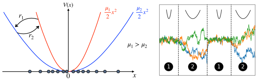
Figure 1: The left panel illustrates the setup where $N$ particles are confined in a harmonic potential $V(x)$, whose stiffness alternates between $\mu_{1}$ and $\mu_{2}$ with rates $r_{1}$ (from $\mu_{1}$ to $\mu_{2}$) and $r_{2}$ (from $\mu_{2}$ to $\mu_{1}$) respectively. On the right, we show the schematic trajectories for $N=3$ diffusing particles. The switching times are shown by dashed vertical black lines.

The stochastic resetting for single particle systems discussed above can be easily generalized to many-body systems. In this case, the whole configuration of the system (i.e., all the degrees of freedom) is reset instantaneously to a pre-decided configuration at random times with rate $r$. This leads to a many-body NESS with interesting spatial structures that have been observed in a number of systems, such as fluctuating interfaces GMS14 , symmetric exclusion process BKP19 , the Ising model MMS20 , etc. Recently, a very simple model of $N$ noninteracting Brownian motions in one dimension, subjected to simultaneous resetting to their initial positions with rate $r$, was introduced BLMS_23 . Remarkably, even though the particles are noninteracting in this model, the simultaneous resetting generates an effective all-to-all attractive interaction between these particles that persists even at long times in the NESS. This model demonstrated an important phenomenon, namely the emergence of strong collective correlations in the steady state of a many-body system, where the interactions between constituents are not built-in but instead emerge from the dynamics itself.

One of the shortcomings of these theoretical models, either for single or multi-particle system, is the assumption of instantaneous resetting Reu_16 ; EM18_ref ; BS_20 ; BS_2_20 ; Sunil23 . While this assumption makes the problem simpler and easy to implement in both numerical simulations and theoretical analysis, it is not very realistic experimentally. For example, in the optical trap experiments of a single diffusing particle with SR, the typical protocol consists of alternative intervals of free diffusion and confined motions BBPMC_20 ; FBPCM_21 . During the free period, the particle is allowed to diffuse freely in the absence of an optical trap. At the end of this period a harmonic trap is switched on and the particle is thermally equilibrated in the trap. Once the particle has equilibrated, the trap is switched off and a new period of free motion starts. In the confined phase, no measurement is performed, since this protocol was designed to mimic the instantaneous resetting move BBPMC_20 ; FBPCM_21 . One may naturally wonder what happens if one does not wait till the full equilibration in the confined phase but instead switches off the trap at a random time, e.g., distributed exponentially.

This leads to a more realistic and general protocol where the particle moves in a harmonic trap whose stiffness switches intermittently between $\mu_{1}$ and $\mu_{2}$ (with $\mu_{1}>\mu_{2}$ without any loss of generality). The stiffness changes from $\mu_{1}$ to $\mu_{2}$ with rate $r_{1}$ and reciprocally with rate $r_{2}$ from $\mu_{2}$ to $\mu_{1}$ (see Fig. 1 for an illustration). In the limit $\mu_{1}\to\infty$, $\mu_{2}\to 0$ and $r_{1}\to\infty$, this general protocol reduces to the standard model of diffusion under SR to the origin. The limit $\mu_{1}\to\infty$ and $\mu_{2}\to 0$ ensures resetting of a diffusing particle to the origin, while the limit $r_{1}\to\infty$ guarantees that once it is reset to the origin, it immediately restarts, thus realising the instantaneous resetting. For a single particle undergoing this switching intermittent potential, the resulting position distribution in the NESS has been studied only recently MBMS_20 ; GPKP_20 ; SDN_21 ; XZMD_22 ; GP_22 ; ACB_22 ; MBM_22 . In this paper, our goal is to study $N$ independent particles undergoing this switching intermittent protocol. One of our main results is to show that, indeed, the switching dynamics between two stiffnesses of the trap drives the system into a NESS with strong collective correlations that emerge purely out of the dynamics. Thus the emergence of strong correlations without direct interaction is a robust phenomenon and is not just an artefact of instantaneous resetting.

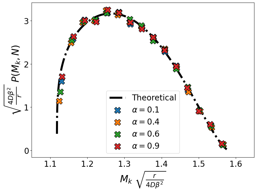
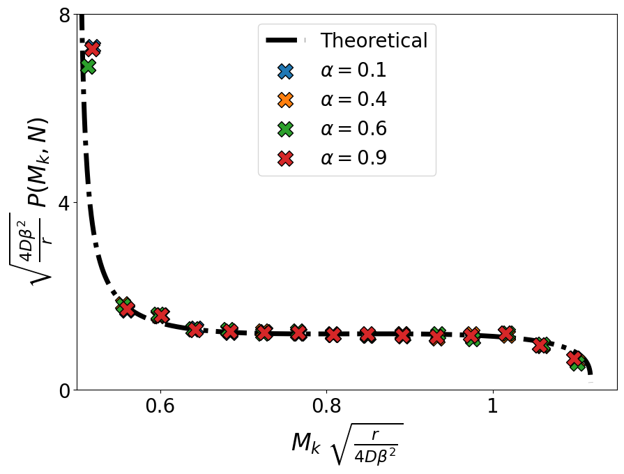
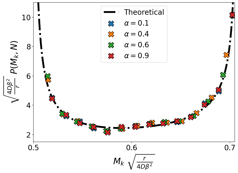
Figure 2: Scaling collapse of the distribution of the $k$-th maximum as in Eq. (17) for different values of $\alpha=k/N$ and different values of the parameters. We set $r_{1}=r_{2}=1$, $D=1$, $N=10^{6}$ and vary $\mu_{1}$ and $\mu_{2}$. From left to right we used respectively $\mu_{1}=0.4,\,\mu_{2}=0.2$ then $\mu_{1}=2,\,\mu_{2}=0.4$ and finally $\mu_{1}=2,\,\mu_{2}=1$. The dashed black line corresponds to the theoretical prediction and the symbols are the numerical results. Different colors correspond to different values of $\alpha$. The numerical results were obtained by sampling $10^{5}$ examples directly from the NESS distribution given in Eq. (12).

Let us first summarize our main results. For $N$ independent particles on the line driven by this switching intermittent protocol, we first provide a complete characterisation of the NESS, i.e., the exact computation of the joint distribution of the positions of the particles. This allows us to compute the spatial correlations in the NESS, as well as several other physical observables, such as the average density, the distribution of the position of the rightmost particle in the gas (extreme value statistics), the spacing distribution between particles and the full counting statistics (FCS), i.e., the statistics of the number of particles in a given interval. These observables have been calculated recently for large $N$ in the limit of instantaneous resetting BLMS_23 but, here, we show that these asymptotic results get drastically modified under this intermittent switching protocol. In particular, we find a surprising result for the extreme value statistics (EVS), i.e., the distribution of the position $M_{1}$ of the rightmost particle. We show that in the large $N$ limit, $M_{1}$ typically scales as $\sqrt{\ln N}$ and its probability distribution function (PDF) takes the scaling form

$${\rm Prob.}\left(M_{1}=w,N\right)\approx\sqrt{\frac{r_{H}}{4D\,\ln N}}f\left(w\sqrt{\frac{r_{H}}{4D\,\ln N}}\right)$$ (1)

where $r_{H}=2/(1/r_{1}+1/r_{2})$ is the harmonic mean of the switching rates and the scaling function $f(z)$ has a nontrivial shape supported over a finite interval $\sqrt{r_{H}/(2\mu_{1})}\leq z\leq\sqrt{r_{H}/(2\mu_{2})}$ [see Eqs. (Dynamically emergent correlations between particles in a switching harmonic trap) and (17) and Fig. 2], even though the average density is supported over the full line (see Fig. 1). By tuning the parameters $r_{1},r_{2},\mu_{1},\mu_{2}$, the shape of this PDF changes drastically as seen in Fig. 2. This is remarkable since in all the known examples of EVS in uncorrelated G_58 ; A_78 ; LLR_82 ; D_85 ; W_88 ; ABN_92 ; ND_03 ; FC_15 or correlated TW_94 ; DM_01 ; CD_01 ; MK_03 ; MC_04 ; MC_05 ; SM_06 ; BC_06 systems (for a recent review see MPS_20 ), including the instantaneous resetting case discussed above, the limiting distribution of the maximum is always supported over an unbounded interval (infinite or semi-infinite). The emergence of a finite support with a tunable shape for the EVS is thus a strong signature of the non-instantaneous nature of this switching protocol. In addition to having a finite support, we find that the scaling function $f(z)$ in Eq. (1) is surprisingly robust and universal: it also describes the scaling of the $k$-th maximum in $d=1$ as well as the distribution of the distance of the farthest particle from the center of a $d$-dimensional harmonic trap. In the rest of the paper, we present only the computation of the joint distribution and the EVS in Eq. (1). The computations of the other observables mentioned above are provided in the Supp. Mat. SM .

The Model. We consider $N$ independent Brownian particles on a line, all starting at the origin which feel a potential that switches between $V_{1}(x)=\mu_{1}x^{2}/2$ and $V_{2}(x)=\mu_{2}x^{2}/2$, with Poissonian rate $r_{1}$ (from $\mu_{1}$ to $\mu_{2}$) and rate $r_{2}$ (from $\mu_{2}$ to $\mu_{1}$). Hence, the duration $\tau$ of the time intervals between successive switches is distributed via ${\rm Prob.}[\tau]=r_{i}e^{-r_{i}\tau}$, where $r_{i}$ is $r_{1}$ or $r_{2}$. Moreover, the intervals are statistically independent. In each phase the positions $\{x_{i}\}$ evolve as independent Ornstein-Uhlenbeck processes UO_30

$$\derivative{x_{i}}{t}=-\mu_{k}x_{i}+\sqrt{2D}\eta_{i}(t)\;,$$ (2)

where $\mu_{k}=\mu_{1}$ or $\mu_{2}$ depending on the phase, $D$ is the diffusion constant and $\eta_{i}(t)$ is a zero-mean Gaussian white noise with a correlator $\langle\eta_{i}(t)\eta_{j}(t^{\prime})\rangle=\delta_{ij}\delta(t-t^{\prime})$. Let $P_{1}(\vec{x},t)$ (resp. $P_{2}$) denote the joint PDF of the particles being at $\vec{x}=(x_{1},\cdots,x_{N})$ at time $t$ and that the system is in phase 1 (resp. phase 2). From Eq. (2), they evolve by the coupled Fokker-Planck equations

$$\partialderivative{P_{1}}{t} =\sum\limits_{i=1}^{N}\left[D\partialderivative[2]{P_{1}}{x_{i}}+\mu_{1}\partialderivative{x_{i}}\left(x_{i}P_{1}\right)\right]-r_{1}P_{1}+r_{2}P_{2}$$ (3)

$$\partialderivative{P_{2}}{t} =\sum\limits_{i=1}^{N}\left[D\partialderivative[2]{P_{2}}{x_{i}}+\mu_{2}\partialderivative{x_{i}}\left(x_{i}P_{2}\right)\right]-r_{2}P_{2}+r_{1}P_{1}$$ (4)

with the initial conditions

$$P_{1}(\vec{x},t=0)=\frac{1}{2}\delta(\vec{x})\mbox{~{}~{}and~{}~{}}P_{2}(\vec{x},t=0)=\frac{1}{2}\delta(\vec{x})\;,$$ (5)

where we assumed that, initially, both phases occur equally likely. Hence the joint PDF of the positions only is given by $P(\vec{x},t)=P_{1}(\vec{x},t)+P_{2}(\vec{x},t)$. The first terms on the right hand side of Eqs. (3) and (4) represent diffusion and advection in a harmonic potential, while the last two terms represent the loss and gain due to the switching between potentials, with rates $r_{1}$ and $r_{2}$ respectively.

To solve this pair of Fokker-Planck equations, it is convenient to work in the Fourier space where we define $\tilde{P}_{n}(\vec{k},t)=\int_{-\infty}^{+\infty}\differential\vec{x}\;e^{i\vec{k}\dot{\vec{x}}}P_{n}(\vec{x},t)$, with $n=1,2$. In the steady state, setting $\partial_{t}\tilde{P}_{n}=0$, Eqs. (3) and (4) in the Fourier space reduce to

$$\left(D\sum\limits_{i=1}^{N}k_{i}^{2}+r_{1}\right)\tilde{P_{1}}+\mu_{1}\sum\limits_{i=1}^{N}k_{i}\partialderivative{\tilde{P_{1}}}{k_{i}} =r_{2}\tilde{P_{2}}$$ (6)

$$\left(D\sum\limits_{i=1}^{N}k_{i}^{2}+r_{2}\right)\tilde{P_{2}}+\mu_{2}\sum_{i=1}^{N}k_{i}\partialderivative{\tilde{P_{2}}}{k_{i}} =r_{1}\tilde{P_{1}}\;,$$ (7)

with initial conditions $\tilde{P_{n}}(\vec{k}=0)=1/2$. Notice that Eqs (6)-(7) are spherically symmetric. It is therefore much easier to move to hyper-spherical coordinates where $k=\sqrt{\sum_{i=1}^{N}k_{i}^{2}}$ is the distance to the origin and $\theta_{i}$, for $i=1,\cdots,N-1$ are the different angular coordinates. Then Eqs. (6)-(7) simplify to

$$\left[(Dk^{2}+r_{1})+\mu_{1}k\partial_{k}\right]\tilde{P_{1}} =r_{2}\tilde{P_{2}}$$ (8)

$$\left[(Dk^{2}+r_{2})+\mu_{2}k\partial_{k}\right]\tilde{P_{2}} =r_{1}\tilde{P_{1}}\;.$$ (9)

Notice that by permuting the indices $1\leftrightarrow 2$ in Eq. (8) leads to Eq. (9). Hence, we can solve only for $\tilde{P_{1}}$ and the solution for $\tilde{P_{2}}$ will follow by permuting the indices. By eliminating $\tilde{P}_{2}$ between Eqs. (8) and (9) we get an ordinary second order differential equation for $\tilde{P}_{1}$ (respectively $\tilde{P}_{2}$). Solving this ordinary differential equations with appropriate boundary conditions (see Supp. Mat. for details) we obtain

$$\tilde{P_{1}}(k)=\frac{r_{2}\,e^{-\frac{Dk^{2}}{2\mu_{1}}}}{r_{1}+r_{2}}M\left(R_{1};1+R_{1}+R_{2};\frac{Dk^{2}(\mu_{2}-\mu_{1})}{2\mu_{1}\mu_{2}}\right),$$ (10)

where $R_{1}=r_{1}/(2\mu_{1})$, $R_{2}=r_{2}/(2\mu_{2})$ and $M(a;b;z)$ is the Kummer’s function NIST . Similarly, one can obtain $\tilde{P}_{2}(\vec{k})$ just by exchanging $\mu_{1}\leftrightarrow\mu_{2}$ and $r_{1}\leftrightarrow r_{2}$. To reveal the spatial correlations in the NESS, it is useful to invert this Fourier transform, which is not easy. However, fortunately, one can make use of a convenient integral representation NIST

$$M(a;b;z)=\frac{\Gamma(b)}{\Gamma(a)\Gamma(b-a)}\int_{0}^{1}\differential u\;e^{zu}u^{a-1}(1-u)^{b-a-1}\;,$$ (11)

where $\Gamma(x)$ is the Gamma function. Using Eq. (11) in Eq. (10) and inverting the Fourier transform we obtain an expression for $P_{1}(\vec{x})$ and similarly for $P_{2}(\vec{x})$. Adding them gives the joint PDF in the NESS SM

$$P^{\rm st}(\vec{x})=\int_{0}^{1}\differential u\;h(u)\prod_{i=1}^{N}p(x_{i}|u)\;,$$ (12)

where

$$h(u)=\frac{c\,r_{H}}{4}u^{R_{1}-1}(1-u)^{R_{2}-1}\left[\frac{1-u}{\mu_{1}}+\frac{u}{\mu_{2}}\right]$$ (13)

with $c=\Gamma(R_{1}+R_{2}+1)/(\Gamma(R_{1}+1)\Gamma(R_{2}+1))$ and $r_{H}=2\,r_{1}r_{2}/(r_{1}+r_{2})$. The function $p(x|u)=e^{-\frac{x^{2}}{2V(u)}}/\sqrt{2\pi V(u)}$ is a pure Gaussian with zero mean and variance $V(u)=D\left(\frac{u}{\mu_{2}}+\frac{1-u}{\mu_{1}}\right)$. This fully characterizes the joint PDF of the positions in the NESS. Note that $h(u)$ is normalised to unity, i.e., $\int_{0}^{1}h(u)\differential u=1$. Thus one can interpret Eq. (12) as the joint distribution of $N$ i.i.d. Gaussian variables with zero mean and a common variance $V(u)$ parametrised by $u$, which itself is a random variable distributed via the PDF $h(u)$. There is indeed a nice physical meaning of this random variable $u$. If the particle was entirely in phase $2$, its stationary distribution would be a Gaussian (the Gibbs state) with a variance $D/\mu_{2}$. In contrast, if it was in phase $1$, it will again be a Gaussian with a variance $D/\mu_{1}$. Hence from the formula $V(u)=D\left(\frac{u}{\mu_{2}}+\frac{1-u}{\mu_{1}}\right)$, one sees that $0\leq u\leq 1$ can be interpreted as the effective fraction of time that each particle spends in phase $2$. This can be put on a more rigorous footing by using the so-called Kesten variables as shown in the Supp. Mat. SM . For simplicity, we will henceforth set $r_{1}=r_{2}=r$ and the results for general $r_{1}\neq r_{2}$ are given in the Supp. Mat. SM .

We note that the joint PDF in Eq. (12) does not factorise, indicating the presence of correlations in the NESS. One can easily calculate the two-point correlation function from Eq. (12) using the fact that, for a fixed $u$, they are i.i.d. variables. The natural correlator $\langle x_{i}x_{j}\rangle-\langle x_{i}\rangle\langle x_{j}\rangle$ for $i\neq j$ vanishes identically since $p(x_{i}|u)$ is Gaussian and hence symmetric in $x_{i}$. The first nonzero correlator for $i\neq j$ is given by

$$\langle x_{i}^{2}x_{j}^{2}\rangle -\langle x_{i}^{2}\rangle\langle x_{j}^{2}\rangle=$$

$$\frac{D^{2}}{r^{2}}\frac{(R_{1}-R_{2})^{2}(2+3R_{1}+3R_{2}+4R_{1}R_{2})}{(1+R_{1}+R_{2})^{2}(2+R_{1}+R_{2})}\;,$$ (14)

where we recall that $R_{1}=r/(2\mu_{1})$ and $R_{2}=r/(2\mu_{2})$. The positive value of this correlator indicates that there are effective all-to-all attractive correlations between the particles in the NESS. These correlations are not built-in but get generated by the switching dynamics of the potential, which all the particles share together. This makes the particles strongly correlated in the NESS. Despite such strong correlations, the structure of the joint PDF in Eq. (12) allows us to compute several physical observables exactly, such as the average density, the EVS, the distribution of the spacings between particles and also the FCS. The reason for the solvability can be traced back to Eq. (12) where one can first fix $u$ and compute the observables for $N$ independent variables, each distributed via $p(x|u)$ where $u$ is just a fixed parameter and then average over $u$ drawn from the PDF $h(u)$ in Eq. (13). For i.i.d. variables, this computation is rather standard. This solvable structure holds more generally for any conditionally independent and identically distributed (c.i.i.d.) variables, as studied recently in Ref. BLMS_23-2 . Here, the c.i.i.d. structure emerges from the basic dynamics of the system and thus provides a natural physical example of such systems. The computation of these physical observables are provided in details in the Supp. Mat. SM and here we focus only on the EVS. This is because the EVS of strongly correlated variables is known to be a very hard problem and there are only few cases where it can be derived analytically. Our model provides not only a solvable example of EVS in a strongly correlated system, but also the distribution of the EVS turns out to be rather surprising as discussed below.

To compute the EVS, we start from the joint PDF in Eq. (12). We first fix $u$ and compute the EVS of $N$ i.i.d. Gaussian random variables of zero mean and variance $V(u)$. It is well known MPS_20 that, for large $N$, the maximum $M_{1}$ of such i.i.d. Gaussian variables behaves almost deterministically as $M_{1}\approx\sqrt{2V(u)\,\ln N}$, with fluctuations around it of order $1/\sqrt{\ln N}$. It turns out that, to leading order for large $N$, one can approximate this distribution by a delta function, namely $P(M_{1}=w|u)\approx\delta(w-\sqrt{2V(u)\,\ln N})$. Finally, averaging over $u$ we get

$$P(M_{1}=w,N)\approx\int_{0}^{1}\differential u\,h(u)\,\delta\left(w-\sqrt{2V(u)\,\ln N}\right)$$ (15)

where $V(u)=D(u/\mu_{2}+(1-u)/\mu_{1})$ and $h(u)$ is given in Eq. (13). Performing this integral explicitly SM , we get the scaling form in Eq. (1) where the scaling function $f(z)$ has a nontrivial shape given by

$$f(z)=\frac{c\,R_{1}^{R_{1}-1}R_{2}^{R_{2}-1}}{(R_{2}-R_{1})^{R_{1}+R_{2}-1}} |z|^{3}$$

$$\left(1-\frac{z^{2}}{R_{2}}\right)^{R_{2}-1} \left(\frac{z^{2}}{R_{1}}-1\right)^{R_{1}-1}\;,$$ (16)

with $\sqrt{R_{1}}\leq z\leq\sqrt{R_{2}}$. As mentioned earlier, an EVS scaling function with a finite support is rather surprising because the average density is spread over the full real line SM . Moreover the shape of the scaling function $f(z)$ can be tuned by varying the parameters $R_{1}$ and $R_{2}$. At both edges of the support $f(z)$ can either diverge, go to a nonzero constant or vanish, depending on $R_{1},R_{2}$. The scaling function $f(z)$ also turns out to be universal in the following sense. If one calculates the distribution of the $k$-th maximum (order statistics), one finds a scaling form

$${\rm Prob.}[M_{k}=w,N]\approx\sqrt{\frac{r_{H}}{4D\beta^{2}}}\;f\left(w\sqrt{\frac{r_{H}}{4D\beta^{2}}}\right)\;,$$ (17)

where $\beta={\rm erfc}^{-1}(2k/N)$, but the scaling function $f(z)$ is independent of $k$ and has the same expression as in Eq. (Dynamically emergent correlations between particles in a switching harmonic trap). Here ${\rm erfc}(z)=2/\sqrt{\pi}\int_{z}^{\infty}e^{-y^{2}}\,\differential y$. In Fig. 2, we verify this scaling form by collapsing data for different $\alpha=k/N$ and for different values of $R_{1}$ and $R_{2}$. The numerical results are in excellent agreement with our theoretical predictions. Furthermore, one can easily generalise our results to a harmonic trap in $d$ dimensions SM . Following exactly the same analysis as in the $d=1$ case above, one can also compute the distribution of the distance of the farthest particle from the center of the trap and we find the remarkable result that it is again described by Eq. (1) with the same scaling function $f(z)$ given in Eq. (Dynamically emergent correlations between particles in a switching harmonic trap). Thus the scaling function $f(z)$ is extremely robust and “super-universal”, in the sense that it neither depends on $k$ in $d=1$ and nor on the dimension $d$ itself.

To summarize, we have completely characterised the nonequilibrium stationary state of $N$ Brownian particles in a harmonic trap in an experimentally realistic protocol where the stiffness of the trap switches between two values at constant rate. The strong correlations between the positions of the particles in the stationary state emerge from the dynamics itself and are not built-in. The exact joint distribution of the particle positions allows us to compute several physical observables analytically. In particular, we have shown that the EVS is characterized by a nontrivial scaling function which has a finite support and a tunable shape. Moreover, the scaling function of the EVS is universal in the sense that it also describes the limiting distribution of the $k$-th maximum in $d=1$ as well as the distribution of the distance of the particle farthest from the center of the harmonic trap in $d$-dimensions SM . It would be interesting if our predictions can be verified experimentally and also to investigate the NESS in non-harmonic traps.

- (1) M. R. Evans, S. N. Majumdar, and G. Schehr, J. Phys. A: Math. Theor. 53, 193001 (2020).
- (2) A. Pal, S. Kostinski, and S. Reuveni, J. Phys. A: Math. Theor. 55, 021001 (2022).
- (3) S. Gupta, and A. M. Jayannavar, Front. Phys. 10 789097, (2022).
- (4) M. R. Evans and S. N. Majumdar, Phys. Rev. Lett. 106, 160601 (2011).
- (5) M. R. Evans and S. N. Majumdar, J. Phys. A: Math. Theor. 44, 435001 (2011).
- (6) O. Tal-Friedman, A. Pal, A. Sekhon, S. Reuveni, and Y. Roichman, J. Phys. Chem. Lett. 11, 7350 (2020).
- (7) B. Besga, A. Bovon, A. Petrosyan, S. N. Majumdar, S. Ciliberto, Phys. Rev. Research 2, 032029(R) (2020).
- (8) F. Faisant, B. Besga, A. Petrosyan, S. Ciliberto, S. N. Majumdar, J. Stat. Mech., 113203 (2021).
- (9) S. Reuveni, M. Urbakh, J. Klafter, Proc. Natl. Acad. Sci. USA. 111, 4391 (2014).
- (10) D. Boyer, C. Solis-Salas, Phys. Rev. Lett. 112, 240601 (2014).
- (11) T. Rotbart, S. Reuveni, M. Urbakh, Phys. Rev. E 92, 060101 (2015).
- (12) S. N. Majumdar, S. Sabhapandit, G. Schehr, Phys. Rev. E 92, 052126 (2015).
- (13) A. Pal, A. Kundu, M. R. Evans, J. Phys. A: Math. Theor. 49, 225001 (2016).
- (14) S. Reuveni, Phys. Rev. Lett. 116, 170601 (2016).
- (15) M. Montero, J. Villarroel, Phys. Rev. E 94, 032132 (2016).
- (16) A. Nagar, S. Gupta, Phys. Rev. E 93, 060102 (2016).
- (17) A. Pal, S. Reuveni, Phys. Rev. Lett. 118, 030603 (2017).
- (18) D. Boyer, M. R. Evans, S. N. Majumdar, J. Stat. Mech. 023208, (2017).
- (19) M. R. Evans and S. N. Majumdar, J. Phys. A: Math. Theor. 51, 475003 (2018).
- (20) A. Chechkin, I. M. Sokolov, Phys. Rev. Lett. 121, 050601 (2018).
- (21) G. Mercado-Vasquez, D. Boyer, J. Phys. A: Math. Theor. 51, 405601 (2018).
- (22) A. Pal, L. Kuśmierz and S. Reuveni, Phys. Rev. E 100 040101 (2019).
- (23) A. Masó-Puigdellosas, D. Campos, V. Méndez, Front. Phys. 7, 112 (2019).
- (24) A. Pal, L. Kusmierz, S. Reuveni, Phys. Rev. Res. 2, 043174 (2020).
- (25) A. S. Bodrova and I. M. Sokolov, Phys. Rev. E 101 052130 (2020).
- (26) A. S. Bodrova and I. M. Sokolov, Phys. Rev. E 102 032129 (2020).
- (27) B. De Bruyne, J. Randon-Furling, and S. Redner, Phys. Rev. Lett. 125, 050602 (2020).
- (28) P. C. Bressloff, J. Phys. A: Math. Theor. 53, 425001 (2020).
- (29) R. G. Pinsky, Stoch. Proc. Appl. 130, 2954 (2020).
- (30) B. De Bruyne, S. N. Majumdar, G. Schehr, Phys. Rev. Lett. 128, 200603 (2022).
- (31) F. Mori, S. N. Majumdar, and G. Schehr, Phys. Rev. E 106, 054110 (2022).
- (32) I. Santra, U. Basu, S. Sabhapandit, J. Phys. A: Math. Theor. 55, 414002 (2022).
- (33) B. De Bruyne, F. Mori, Phys. Rev. Res. 5, 013122 (2023).
- (34) M. Biroli, S. N. Majumdar, and G. Schehr, Phys. Rev. E 107, 064141 (2023).
- (35) F. Mori, K. S. Olsen, and S. Krishnamurthy, Phys. Rev. Res. 5, 023103 (2023).
- (36) S. Gupta, S. N. Majumdar, and G. Schehr, Phys. Rev. Lett. 112, 220601 (2014).
- (37) U. Basu, A. Kundu, and A. Pal., Phys. Rev. E 100, 032136 (2019).
- (38) M. Magoni, S. N. Majumdar and G. Schehr, Phys. Rev. Res. 2, 033182 (2020).
- (39) M. Biroli, H. Larralde, S. N. Majumdar, and G. Schehr, Phys. Rev. Lett. 130, 207101 (2023)
- (40) M. R. Evans and S. N. Majumdar, J. Phys. A: Math. Theor. 52, 01LT01 (2018).
- (41) J. C. Sunil, R. A. Blythe, M. R. Evans, and S. N. Majumdar, J. Phys. A: Math. Theor. 56, 395001 (2023).
- (42) G. Mercado-Vasquez, D. Boyer, S. N. Majumdar, G. Schehr, J. Stat. Mech., 113203 (2020).
- (43) D. Gupta, C. A. Plata, A. Kundu and A. Pal, J. Phys. A: Math. Theor. 54 025003 (2020)
- (44) I. Santra, S. Das and S. K. Nath, J. Phys. A: Math. Theor. 54 334001 (2021)
- (45) P. Xu, T. Zhou, R. Metzler and W. Deng, New J. Phys. 24 033003 (2022)
- (46) D. Gupta and C. A. Plata, New J. Phys. 24, 113034 (2022).
- (47) H. Alston, L. Cocconi and T. Bertrand, J. Phys. A: Math. Theor. 55 274004 (2022)
- (48) G. Mercado-Vàsquez, D. Boyer, S. N. Majumdar, J. Stat. Mech. 093202 (2022)
- (49) E.J. Gumbel, Statistics of Extremes (Dover), (1958).
- (50) C.W. Anderson, J.R. Statist. Soc. B40, 197-202 (1978).
- (51) M.R. Leadbetter, G. Lindgren, and H. Rootzen, Extremes and related properties of random sequences and processes, Springer-Verlag, New York, (1982).
- (52) B. Derrida, J. Phys. Lett. 46, 401 (1985).
- (53) I. Weissman, Adv. Appl. Probab. 20, 8 (1988).
- (54) B.C. Arnold, N. Balakrishnan and H.N. Nagaraja, A first course in order statistics, Wiley, New York (1992).
- (55) H.N. Nagaraja, H.A. David, Order statistics (third ed.), Wiley, New Jersey (2003).
- (56) J. Y. Fortin, M. Clusel, J. Phys. A: Math. Theor. 48, 183001 (2015).
- (57) C.A. Tracy, H. Widom, Commun. Math. Phys. 159, 151 (1994).
- (58) D. Carpentier and P. Le Doussal, Phys. Rev. E 63, 026110 (2001).
- (59) D.S. Dean, S.N. Majumdar, Phys. Rev. E 64, 046121 (2001).
- (60) S. N. Majumdar, P. L. Krapivsky, Physica A 318, 161 (2003).
- (61) S.N. Majumdar, A. Comtet, Phys. Rev. Lett. 92, 225501 (2004).
- (62) S.N. Majumdar, A. Comtet, J. Stat. Phys. 119, 777 (2005).
- (63) G. Schehr, S.N. Majumdar, Phys. Rev. E 73, 056103 (2006).
- (64) E. Bertin, M. Clusel, J. Phys. A: Math. Gen. 39, 7607 (2006).
- (65) S.N. Majumdar, A. Pal, and G. Schehr, Phys. Rep. 840, 1 (2020).
- (66) M. Biroli, M. Kulkarni, S. N. Majumdar, G. Schehr, Supplementary Material.
- (67) G. E. Uhlenbeck and L. S. Ornstein, Phys. Rev. 36, 823 (1930).
- (68) F. W. J. Olver, D. W. Lozier, R. F. Boisvert and C. W. Clark. The NIST Handbook of Mathematical Functions. Cambridge University Press (2010).
- (69) M. Biroli, H. Larralde, S.N. Majumdar, G. Schehr, arXiv preprint arXiv:2307.15351 (2023)