Think Twice Before Selection: Federated Evidential Active Learning for Medical Image Analysis with Domain Shifts

Abstract

Federated learning facilitates the collaborative learning of a global model across multiple distributed medical institutions without centralizing data. Nevertheless, the expensive cost of annotation on local clients remains an obstacle to effectively utilizing local data. To mitigate this issue, federated active learning methods suggest leveraging local and global model predictions to select a relatively small amount of informative local data for annotation. However, existing methods mainly focus on all local data sampled from the same domain, making them unreliable in realistic medical scenarios with domain shifts among different clients. In this paper, we make the first attempt to assess the informativeness of local data derived from diverse domains and propose a novel methodology termed Federated Evidential Active Learning (FEAL) to calibrate the data evaluation under domain shift. Specifically, we introduce a Dirichlet prior distribution in both local and global models to treat the prediction as a distribution over the probability simplex and capture both aleatoric and epistemic uncertainties by using the Dirichlet-based evidential model. Then we employ the epistemic uncertainty to calibrate the aleatoric uncertainty. Afterward, we design a diversity relaxation strategy to reduce data redundancy and maintain data diversity. Extensive experiments and analyses are conducted to show the superiority of FEAL over the state-of-the-art active learning methods and the efficiency of FEAL under the federated active learning framework.

1 Introduction

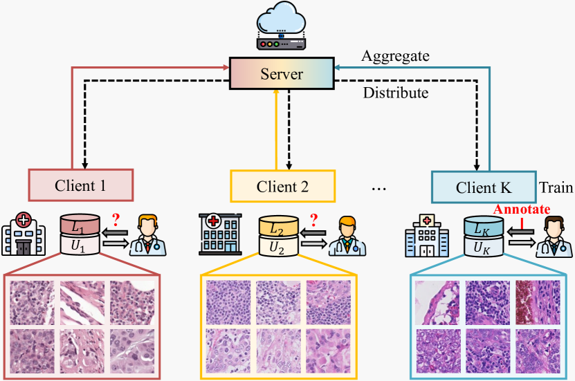
(a) FAL scheme

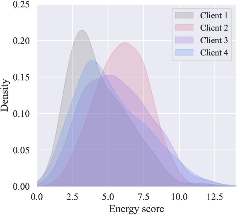
(b) KDE of energy score

(c) $p$-value

Figure 1: Illustration of federated active learning (FAL) in the presence of domain shift. (a) FAL comprises model distribution, local training, model aggregation, and data annotation. (b) The KDE of energy scores depicts domain shifts across clients. (c) The low $p$-values in cross-client KDE of energy scores indicate the existence of significant domain shifts between all client pairs.

Federated learning enables collaborative learning across multiple clinical institutions (i.e., clients) to learn a unified model on the central server through model aggregation while preserving the data privacy at each client [23, 34, 55] (see Fig. 1 (a)). Unfortunately, such a learning pipeline requires each client to prepare its own labeled data, whose scale is constrained by the available expertise, time, and budget for data annotation.

One possible solution to alleviate the annotation cost is to select a part of highly informative data to annotate. Active learning (AL) has shown great potential in guiding the data selection process [1, 58, 21, 6], leading to the federated AL (FAL) framework. Such a pipeline [35, 44, 60, 16, 7, 40] allows each client to assess the informativeness of unlabeled data using either the local model at each client or the global model from the server, greatly alleviating the heavy annotation costs while retaining great performance. Nevertheless, when using a local model to select data, there is a bias toward prioritizing the data that improves the local updates while disregarding the overall generalizability of the global model. Client models trained on diverse domains may exhibit significant divergence within the parameter space, making the use of a global model aggregated from these models for data selection unreliable.

Recent advances in FAL, e.g., LoGo [21] and KAFAL [6], tend to harness the knowledge of both local and global models to identify informative samples. Although this strategy has been proven to be more effective than employing a single model, these methods focus mainly on the class imbalance issue while assuming that the data at multiple clients is from the same domain. However, the domain shift across clients is commonly seen in real-world applications, which is evidenced by the extremely low $p$-values of the kernel density estimation (KDE) of energy scores [32] (see Fig. 1 (b) and (c)). The existence of domain shift renders two major challenges for FAL. (1) Overconfidence; Existing FAL methods evaluate data uncertainty based on the softmax prediction made by a deterministic model, which is essentially a point estimate and can be miscalibrated easily on data with domain shifts [32, 41], resulting in unreliable uncertainty evaluation. (2) Limited uncertainty representation. Uncertainty can be divided into aleatoric uncertainty (or data uncertainty) and epistemic uncertainty (or knowledge uncertainty) [42]. The former reflects the inherent complexity of data, such as class overlap and instance noise [52]. The latter captures the restricted knowledge of a model caused by insufficient data or domain shifts. The softmax prediction can represent the aleatoric uncertainty but fails to capture the epistemic uncertainty, resulting in incomplete evaluations, which are particularly noticeable in the presence of domain shift.

To address both challenges, we propose the Federated Evidential Active Learning (FEAL) method. Built upon the Dirichlet-based evidential model, FEAL treats the categorical prediction of a sample as following a Dirichlet distribution, thus allowing multiple potential predictions for a sample. FEAL comprises two key modules, i.e., calibrated evidential sampling (CES) and evidential model learning (EML). CES is a novel FAL sampling strategy that incorporates both uncertainty and diversity measures. It utilizes the expected entropy of potential predictions to quantify aleatoric uncertainty and aggregates the aleatoric uncertainty in both global and local models. Further, CES employs the differential entropy of the Dirichlet distribution to characterize the epistemic uncertainty and utilizes the epistemic uncertainty in the global model to calibrate the aggregated aleatoric uncertainty. To enhance data selection, diversity relaxation is also employed with the local model to reduce redundancy and maintain diversity among the selected samples. In addition to active sampling, we introduce evidence regularization in EML for accurate evidence representation and data assessment. The main contributions of this work are summarized as follows:

• We explore a rarely studied problem, FAL with domain shifts, which aims to attain a global model with a limited annotation budget for each local client in the presence of domain shifts.

• We propose the FEAL method, with a sampling strategy CES and a local training scheme EML, to tackle the challenges in FAL with domain shifts. CES is designed to select informative samples by leveraging aleatoric and epistemic uncertainty with both global and local models and retaining sample diversity. EML is developed to regularize the evidence for improved data evaluation.

• We conduct extensive experiments on five real multi-center medical image datasets, comprising two datasets for classification and three datasets for segmentation. The results suggest the superiority of our FEAL method over its AL and FAL counterparts.

2 Related Work

2.1 Federated Learning with Domain Shifts

Domain shift is a long-standing challenge for federated learning. Liu et al. [31] transmitted the domain information across clients through continuous frequency space interpolation. However, the transmit operations can introduce additional costs and risks of data privacy leakage. Li et al. [29] observed that a portion of the domain-specific information is concealed within the batch normalization (BN) layer, and they suggested aggregating non-BN layers to obtain a robust global model. Li et al. [28] and Huang et al. [17] emphasized the use of personalized models over a shared global model to enhance model generalization. However, both of these approaches necessitate the inclusion of additional discriminators and public data, which can impose a significant computational burden on either the participant or the server side. Huang et al. [18] tackled the domain shift issue using prototype learning, incorporating cluster prototypes and unbiased prototypes for feature regularization. Zhang et al. [62] dynamically tailored model aggregating weights of local models to compensate for the generalization gaps between global and local models caused by domain shift. These approaches strive to mitigate the impact of domain shifts across clients in supervised scenarios with fully annotated training samples. They ignore the heavy annotation costs for each client. Unlike them, we further leverage active learning to reduce costs by selecting the most informative data and propose a label-efficient method for federated learning with domain shifts.

2.2 AL Methods

Conventional AL methods can be categorized into uncertainty-based, diversity-based, and hybrid ones. Uncertainty-based AL methods aim to select the most ambiguous unlabeled samples for annotation. Classical approaches such as least confidence sampling [46], margin-based sampling [35], and entropy-based sampling [47] evaluate the data uncertainty based on categorical probabilities. Yoo et al. [60] and Huang et al. [16] estimated the loss for uncertainty assessment. Moreover, several approaches assess the data uncertainty by analyzing the prediction inconsistency among multiple augmented samples [14], standard and dropout inferences [12, 13], or original and disturbed features [40]. Diversity-based AL methods aim to identify a subset of samples that captures the distribution of the complete dataset. A variety of approaches have been proposed that exploit core-set techniques [44, 7] or clustering methods [37, 25, 53] in the latent feature space, incorporate a diversity constraint in the optimization process [10, 59], or model the distribution discrepancy between labeled and unlabeled samples [27] in order to identify a diverse collection of samples. Hybrid AL methods exploit both uncertainty and diversity in their sampling strategies. Ash et al. [2] clustered the gradient embeddings to guarantee both uncertainty and diversity. A two-stage sampling strategy has also been implemented [40, 54, 61]. However, these methods primarily focus on data selection driven by aleatoric uncertainty, often neglecting its sufficiency and reliability in practical scenarios. In this work, we developed a Dirichlet-based evidential model to capture both aleatoric and epistemic uncertainties. We further leveraged the epistemic uncertainty to calibrate uncertainty estimates, enhancing their reliability in the context of domain shifts.

2.3 FAL Methods

FAL aims to enhance the annotation efficacy of each local client in decentralized learning. In contrast to the centralized scenarios, there exist two potential query-selector models in FAL, including the global model and the local model. Both Wu et al. [58] and Ahn et al. [1] exclusively utilized a singular model for data evaluation. Specifically, Wu et al. [58] introduced a hybrid metric that considers both the locally predicted loss and the local feature distances between unlabeled and labeled samples. By contrast, Ahn et al. [1] argued that evaluating samples with the global model contributes to the objectives of federated learning and recommended applying sampling strategies solely with the global model. Nevertheless, as demonstrated in [21], the superiority of the two query-selector models depends on the global and local heterogeneous levels, and it is necessary to leverage the knowledge of both global and local models. Kim et al. [21] proposed a hybrid metric called LoGo, which applies $k$-means clustering technique [33] on the gradient space of the local model and subsequently conducts cluster-wise sampling using the global model. Cao et al. [6] proposed a knowledge-specialized sampling strategy, which leverages the discrepancy between the global model and local model to assess data uncertainty. However, these methods focus on the local data from a singular domain, which is less realistic. Though partial approaches [21, 6] account for heterogeneity caused by class imbalance, they often neglect another heterogeneous property known as domain shifts. In this work, we propose the uncertainty calibration method to achieve reliable uncertainty evaluation with domain shifts across multiple clients.

3 Methodology

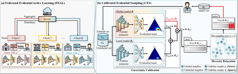
Figure 2: Illustration of the proposed FEAL method. (a) Overview of FEAL. Local client $k$ assesses unlabeled samples’ informativeness using the global model $\boldsymbol{\theta}$ and its local model $\boldsymbol{\theta}_{k}$ in data annotation. (b) Illustration of CES module. In uncertainty calibration, the aggregated aleatoric uncertainty $U_{\text{ale}}(\boldsymbol{x},\boldsymbol{\theta})+U_{\text{ale}}(\boldsymbol{x},\boldsymbol{\theta}_{k})$ is calibrated by the epistemic uncertainty $U_{\text{epi}}(\boldsymbol{x},\boldsymbol{\theta})$. In diversity relaxation, the candidate sample $\boldsymbol{x}_{i}$ would be ignored if its neighbor account meets the minimum neighbor size $n$ and at least one neighbor is already annotated.

3.1 Problem Formulation

The overview of our FEAL framework is displayed in Fig. 2. Under this framework, we maintain $K$ local models $\{\boldsymbol{\theta}_{k}\}_{k=1}^{K}$ on clients and a global model $\boldsymbol{\theta}$ on the central server. The $k$-th local client contains a labeled set $L_{k}$ and an unlabeled set $U_{k}$. FAL comprises two iterative phases: federated model training and local data annotation. Federated model training involves model distribution, local training, and model aggregation. In the first round, the $k$-th client randomly selects $B_{k}$ unlabeled samples and annotates them to form the initial labeled set $L_{k}^{1}=\{(\boldsymbol{x}_{i},\boldsymbol{y}_{i})\}_{i=1}^{B_{k}}$, and the unlabeled set is updated to $U_{k}^{1}=U_{k}\setminus L_{k}^{1}$. In the $r$-th FAL round, the $k$-th client uses a data evaluation strategy to construct the query set $Q_{k}^{r}=\{(\boldsymbol{x}_{j},\boldsymbol{y}_{j})\}_{j=1}^{B_{k}}$ for annotation and update the labeled set to $L_{k}^{r}=L_{k}^{r-1}\cup Q_{k}^{r}$, whereas the unlabeled set is updated to $U_{k}^{r}=U_{k}^{r-1}\setminus Q_{k}^{r}$. Subsequent federated model training proceeds with the updated labeled set $L_{k}$. The FAL process is repeated for $R$ times as required.

3.2 Dirichlet-based Evidential Model in FAL

For federated active learning, we employ a Dirichlet-based evidential model to effectively capture aleatoric and epistemic uncertainties in both global and local models. In this section, we begin by presenting the foundational formulation of the Dirichlet-based evidential model.

We start with the general $C$-class classification task. Given an input sample $\boldsymbol{x}$ from the $k$-th client and a model $f$ parameterized with $\boldsymbol{\theta}$ project $\boldsymbol{x}$ into a $C$-dimensional logits $f(\boldsymbol{x},\boldsymbol{\theta})$. The classical CNN utilizes the softmax operator to transform the logits $f(\boldsymbol{x},\boldsymbol{\theta})$ into the prediction of class probabilities $\boldsymbol{\rho}$. However, this approach essentially provides a single-point estimate of $\boldsymbol{\rho}$ and can be easily miscalibrated on local data from diverse domains. The Dirichlet-based evidential model, on the other hand, views the categorical prediction $\boldsymbol{\rho}$ as a random variable with a Dirichlet distribution $Dir(\boldsymbol{\rho}|\boldsymbol{\alpha})$. The probability density function of $\boldsymbol{\rho}$, given $\boldsymbol{x}$ and $\boldsymbol{\theta}$, is formulated as:

$$p(\boldsymbol{\rho}|\boldsymbol{x},\boldsymbol{\theta})=\left\{\begin{aligned} \frac{\Gamma(\sum_{c=1}^{C}\alpha_{c})}{\prod_{c=1}^{C}\Gamma(\alpha_{c})}\prod_{c=1}^{C}\boldsymbol{\rho}_{c}^{\alpha_{c}-1}&,(\boldsymbol{\rho}\in\Delta^{C})\\ 0\qquad\qquad&,(\text{otherwise})\end{aligned}\right.$$ (1)

where $\alpha$ denotes the parameters of the Dirichlet distribution for sample $\boldsymbol{x}$, $\Gamma(\cdot)$ is the Gamma function, and $\Delta^{C}=\{\boldsymbol{\rho}|\sum_{c=1}^{C}\rho_{c}=1$ and $\forall\rho_{c},0<\rho_{c}<1\}$ represents the $C$-dimensional unit simplex.

The posterior probability $P(y=c|\boldsymbol{x},\boldsymbol{\theta})$ for class $c$, a.k.a., the expected categorical prediction $\overline{\rho}_{c}$, is given by:

$$\small P(y=c|\boldsymbol{x},\boldsymbol{\theta})=\int p(y=c|\boldsymbol{\rho})\cdot p(\boldsymbol{\rho}|\boldsymbol{x},\boldsymbol{\theta})\ \text{d}\boldsymbol{\rho}=\frac{\alpha_{c}}{S},$$ (2)

where $S=\sum_{c=1}^{C}\alpha_{c}$ represents the Dirichlet strength. The derivation of Eq. 2 is provided in Appendix A.1.

Drawing on concepts from Dempster-Shafer theory [45] and subjective logic [20], the parameter $\boldsymbol{\alpha}$ is linked to the accumulated evidence $\boldsymbol{e}$ which quantifies the degree of support for the prediction on the sample $\boldsymbol{x}$. The parameter $\boldsymbol{\alpha}$ is derived as follows:

$$\small\boldsymbol{\alpha}=\boldsymbol{e}+1=\mathcal{A}(f(\boldsymbol{x},\boldsymbol{\theta}))+1,$$ (3)

where $\mathcal{A}(\cdot)$ is a non-negative activation function that transforms the logits $f(\boldsymbol{x},\boldsymbol{\theta})$ into evidence $\boldsymbol{e}$.

All local models adopt the same Dirichlet-based evidential architecture with the global model to communicate between local clients and the central server.

3.3 Calibrated Evidential Sampling

In the context of FAL with domain shifts, we integrate both uncertainty and diversity measures to identify the most informative samples for annotation (see Fig. 2(b)). As for uncertainty evaluation, we leverage the epistemic uncertainty in the global model to calibrate the basic aleatoric uncertainty in both global and local models. We now delve into it details.

Aleatoric uncertainty

Dirichlet-based evidential models interpret the categorical prediction $\boldsymbol{\rho}$ as a distribution rather than a singular point estimate, which acknowledges a range of possible predictions. We use the expected entropy of all possible predictions to deliver the aleatoric uncertainty to quantify the inherent complexity or ambiguity present in local data. Given a sample $\boldsymbol{x}$ and the global model $\boldsymbol{\theta}$, the aleatoric uncertainty of the sample $\boldsymbol{x}$ in the global model $\boldsymbol{\theta}$ is represented as:

$$U_{\text{ale}}(\boldsymbol{x},\boldsymbol{\theta}) =\mathbb{E}_{p(\boldsymbol{\rho}|\boldsymbol{x},\boldsymbol{\theta})}[\mathcal{H}[P(y|\boldsymbol{\rho})]]$$ (4)

$$=\sum_{c=1}^{C}\frac{\alpha_{c}}{S}\cdot[\psi(S+1)-\psi(\alpha_{c}+1)],$$

where $\mathcal{H}(\cdot)$ denotes the Shannon entropy [47]. Similarly, the aleatoric uncertainty in the local model $k$ is $U_{\text{ale}}(\boldsymbol{x},\boldsymbol{\theta}_{k})$. The derivation of Eq. 4 is in Appendix A.2.

Epistemic uncertainty

In the Dirichlet distribution, the differential entropy quantifies how dispersed the probabilities are across different categories. We employ the differential entropy of the Dirichlet distribution to quantify the epistemic uncertainty linked to domain shifts between the global model and local data. Specifically, given a sample $\boldsymbol{x}$ and the global model $\boldsymbol{\theta}$, the epistemic uncertainty of the sample $\boldsymbol{x}$ in the global model $\boldsymbol{\theta}$ is represented as:

$$U_{\text{epi}}(\boldsymbol{x},\boldsymbol{\theta}) =\mathcal{H}[p(\boldsymbol{\rho}|\boldsymbol{x},\boldsymbol{\theta})]$$ (5)

$$=-\int p(\boldsymbol{\rho}|\boldsymbol{x},\boldsymbol{\theta})\cdot\log p(\boldsymbol{\rho}|\boldsymbol{x},\boldsymbol{\theta})\ \text{d}\boldsymbol{\rho}$$

$$=\sum_{c=1}^{C}\log\frac{\Gamma(\alpha_{c})}{\Gamma(S)}-\sum_{c=1}^{C}(\alpha_{c}-1)\cdot[\psi(\alpha_{c})-\psi(S)].$$

The derivation of Eq. 5 is in Appendix A.2.

Uncertainty calibration

Given a sample $\boldsymbol{x}$, the global model $\boldsymbol{\theta}$ and local model $\boldsymbol{\theta}_{k}$, we calculate the aleatoric uncertainty (Eq. 4) in both global and local models and subsequently calibrate the aggregated aleatoric uncertainty by incorporating the epistemic uncertainty (Eq. 5) from the global model. Therefore, the overall calibrated uncertainty for sample $\boldsymbol{x}$ is

$$\small U(\boldsymbol{x},\boldsymbol{\theta},\boldsymbol{\theta}_{k})=[U_{\text{ale}}(\boldsymbol{x},\boldsymbol{\theta})+U_{\text{ale}}(\boldsymbol{x},\boldsymbol{\theta}_{k})]\cdot U_{\text{epi}}(\boldsymbol{x},\boldsymbol{\theta}).$$ (6)

Diversity relaxation

We adopt local constraints to ensure diversity among selected samples, contrasting with core-set techniques that impose global diversity constraints. As outlined in Algorithm 1, we initiate by arranging the unlabeled set $U_{k}^{r-1}$ in descending order of the calibrated uncertainty $U(\boldsymbol{x},\boldsymbol{\theta},\boldsymbol{\theta}_{k})$, and then extract feature embeddings with local model $\boldsymbol{\theta}_{k}$. In the iterative process over the unlabeled set $U_{k}^{r-1}$, we compute the cosine similarity $s(\boldsymbol{x}_{i},\boldsymbol{x}_{j})$ for each candidate sample $\boldsymbol{x}_{i}$ against all other samples $\boldsymbol{x}_{j}\in U_{k}^{r-1}\setminus\boldsymbol{x}_{i}$ and form a neighbor set $N(\boldsymbol{x}_{i})$ based on a predefined similarity threshold $\tau$. A sample $\boldsymbol{x}_{i}$ is selected if its neighbor count $|N(\boldsymbol{x}_{i})|$ is less than the minimum neighbor size $n$ or if these neighbors remain unlabeled. Following this criterion, $B_{k}$ unlabeled samples are chosen to constitute the final set $Q_{k}^{r}$ for annotation, effectively balancing diversity and uncertainty in data selection.

Algorithm 1 Diversity Relaxation for Local Client $k$

0:  unlabeled set $U_{k}^{r-1}$, local model $\boldsymbol{\theta}_{k}$, annotation budget $B_{k}$, similarity threshold $\tau$, minimum neighbor size $n$

0:  query set $Q_{k}^{r}$

1:  Sort $U_{k}^{r-1}$ by descending calibrated uncertainty.

2:  Initialize index $i=1$ and query set $Q_{k}^{r}=\emptyset$.

3:  while $|Q_{k}^{r}|<B_{k}$ and $i\leq|U_{k}^{r-1}|$ do

4:     Select a candidate sample $\boldsymbol{x}_{i}$ from $U_{k}^{r-1}$.

5:     Compute feature similarity $s(\boldsymbol{x}_{i},\boldsymbol{x}_{j})$ using $\boldsymbol{\theta}_{k}$, where $\boldsymbol{x}_{j}\in U_{k}^{r-1}\setminus\boldsymbol{x}_{i}$.

6:     Form neighbor set $N(\boldsymbol{x}_{i})$, including $\boldsymbol{x}_{j}$ with $\!s(\boldsymbol{x}_{i},\boldsymbol{x}_{j})$$\geq$$\tau\!$.

7:     if $|N(\boldsymbol{x}_{i})|<n$ or $N(\boldsymbol{x}_{i})\cap Q_{k}^{r}=\emptyset$ then

8:        Add $\boldsymbol{x}_{i}$ to $Q_{k}^{r}$.

9:     end if

10:     Increment $i$.

11:  end while

12:  return  $Q_{k}^{r}$

3.4 Evidential Model Learning

Dirichlet-based evidential models treat the categorical prediction of a sample as a distribution, enabling a range of potential predictions to occur with specific probabilities. Considering all possible predictions, we adopt the Bayes risk of cross-entropy loss as the task loss for classification tasks. Given an input pair $(\boldsymbol{x},\boldsymbol{y})$ and the local model $\boldsymbol{\theta}_{k}$, the task loss for classification is defined as:

$$\mathcal{L}_{\text{task}}(\boldsymbol{x},\boldsymbol{\theta}_{k},\boldsymbol{y}) =\int[\sum_{c=1}^{C}-y_{c}\log{\rho_{c}}]\cdot p(\boldsymbol{\rho}|\boldsymbol{x},\boldsymbol{\theta}_{k})\ \text{d}\boldsymbol{\rho}$$ (7)

$$=\sum_{c=1}^{C}y_{c}\cdot[\psi(S)-\psi(\alpha_{c})],$$

where $\psi(\cdot)$ is the digamma function and $y_{c}$ is the label indicator for class $c$. Similarly, the Bayes risk of Dice loss for segmentation tasks is:

$$\mathcal{L}_{\text{task}}(\boldsymbol{x},\boldsymbol{\theta}_{k},\boldsymbol{y}) =\int[1-\frac{2}{C}\sum_{c=1}^{C}\frac{\sum_{m=1}^{M}y_{mc}\cdot\rho_{mc}}{\sum_{m=1}^{M}(y_{mc}^{2}+\rho_{mc}^{2})}]\cdot p(\boldsymbol{\rho}|\boldsymbol{x},\boldsymbol{\theta}_{k})\ \text{d}\boldsymbol{\rho}$$ (8)

$$=1-\frac{2}{C}\sum_{c=1}^{C}\frac{\sum_{m=1}^{M}y_{mc}\cdot\overline{\rho}_{mc}}{\sum_{m=1}^{M}[y_{mc}^{2}+\overline{\rho}_{mc}^{2}+\frac{\overline{\rho}_{mc}(1-\overline{\rho}_{mc})}{S_{m}+1}]}.$$

where $\boldsymbol{x}$ is comprised of $M$ pixels and the expected categorical probability for pixel $x_{m}$ is $\overline{\rho}_{mc}=\frac{\alpha_{mc}}{S_{m}}$. The derivation of Eq. 7 and Eq. 8 are in Appendix A.3.

We incorporate evidence regularization to further reduce incorrect evidence and improve correct evidence.

$$\small\mathcal{L}_{\text{reg}}(\boldsymbol{x},\boldsymbol{\theta}_{k},\boldsymbol{y})=KL[Dir(\boldsymbol{\rho}|\tilde{\boldsymbol{\alpha}})\|Dir(\boldsymbol{\rho}|\boldsymbol{1})]-\frac{C}{S}\cdot f(\boldsymbol{x},\boldsymbol{\theta}_{k}),$$ (9)

where $\tilde{\boldsymbol{\alpha}}=\boldsymbol{y}+(\boldsymbol{1}-\boldsymbol{y})\odot\boldsymbol{\alpha}$ and $KL(\cdot)$ denotes the Kullback-Leibler divergence [24]. Notably, we calculate the average pixel-wise $\mathcal{L}_{\text{reg}}$ in segmentation.

The overall training objective, combining task loss $\mathcal{L}_{\text{task}}$ and evidence regularization $\mathcal{L}_{\text{reg}}$, is formulated as:

$$\small\mathcal{L}(\boldsymbol{x},\boldsymbol{\theta}_{k},\boldsymbol{y})=\mathcal{L}_{\text{task}}(\boldsymbol{x},\boldsymbol{\theta}_{k},\boldsymbol{y})+\lambda\cdot\mathcal{L}_{\text{reg}}(\boldsymbol{x},\boldsymbol{\theta}_{k},\boldsymbol{y}).$$ (10)

where $\lambda$ is the trade-off weight between the task loss and the regularization term.

4 Experiments

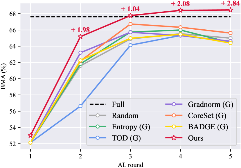
(a) Fed-ISIC (global model)

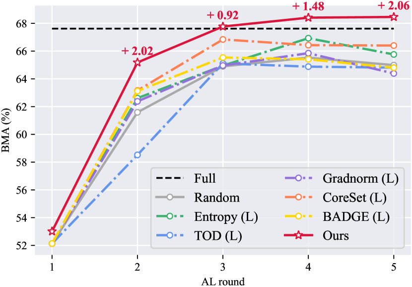
(b) Fed-ISIC (local model)

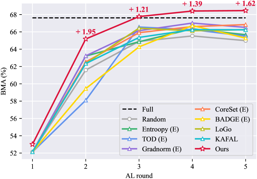
(c) Fed-ISIC (global and local models)

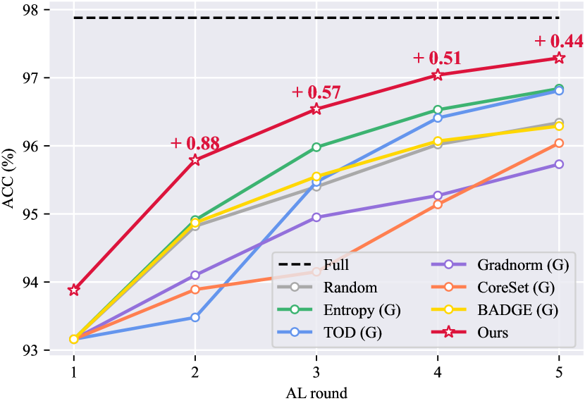
(d) Fed-Camelyon (global model)

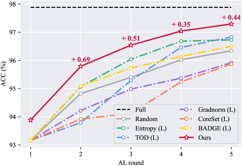
(e) Fed-Camelyon (local model)

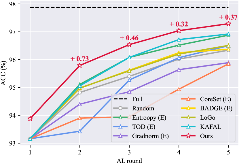
(f) Fed-Camelyon (global and local models)

Figure 3: Comparison of FAL methods in medical image classification. (a)-(c) and (d)-(f) depict the results of the Fed-ISIC and Fed-Camelyon datasets, respectively. Performance enhancements over the second-best method in each FAL round are emphasized in red text.

4.1 Experimental Settings

Datasets

We evaluated FEAL on five real multi-center medical image datasets, encompassing two classification and three segmentation datasets. The classification datasets included

• Fed-ISIC: A skin lesion dataset from 4 data sources [38] containing {9930, 3163, 2691, 1807} images.

• Fed-Camelyon: A breast cancer histology dataset from 5 centers [19] comprising {59436, 30904, 85054, 129838, 146722} patches.

The segmentation datasets included

• Fed-Polyp: A endoscopic polyp dataset from 4 centers [55] with {1000, 380, 196, 612} samples.

• Fed-Prostate: A prostate MRI dataset from 6 data sources [31] with {261, 384, 158, 468, 421, 175} slices.

• Fed-Fundus: A retinal fundus dataset from 4 centers [31] with {101, 159, 400, 400} samples.

In our study, each dataset was divided using an 8:2 train-to-test split ratio at the patient level. Detailed descriptions of these datasets are provided in Appendix B.1.

Evaluation metrics

For classification, we utilized the Balanced Multi-class Accuracy (BMA) for skin lesion classification [8] and measured accuracy (ACC) for breast cancer histology classification. In the context of segmentation, we used the Dice score and the 95% Hausdorff Distance (HD95) to assess segmentation results.

Implementation details

We conducted $R=5$ rounds of FAL involving federated model training and data annotation. During model training, we followed the previous work [57, 19, 55] to utilize EfficientNet-B0 [51] for the Fed-ISIC dataset, DenseNet-121 [15] for the Fed-Camelyon dataset, and U-Net [43] for segmentation datasets. Notably, both EfficientNet-B0 and DenseNet-121 were pre-trained on ImageNet [9]. Each experiment was conducted three times using different random seeds, and the average results were reported. More details are in Appendix B.1.

Comparison methods

We compared FEAL with eight FAL methods, including random sampling (Random), entropy-based sampling (Entropy) [47], TOD [16], Gradnorm [56], CoreSet [44], BADGE [2], LoGo [21], and KAFAL [6]. The first six strategies are primarily developed for standard active learning, whereas LoGo and KAFAL are specifically tailored for decentralized scenarios. To incorporate these standard AL strategies into the FAL framework, we implemented them in three distinct manners: using only the global model (referred to as $G$), depending solely on the local model ($L$), or employing a simple ensemble method with both models ($E$). It guarantees a comprehensive evaluation of these strategies in FAL. The details of comparison methods are summarized in Appendix B.1.

4.2 Results

Table 1: Comparison of FAL methods in medical image segmentation. Dice scores for three segmentation datasets are reported. For the Fed-Fundus dataset, Dice scores for both optic disc and optic cup segmentation and their average are presented. $G$ and $L$ stand for sampling solely with the global or local model, while $E$ represents sampling with both global and local models. Red and blue highlight the Top-1 and Top-2 results, respectively.

		Fed-Polyp (%)				Fed-Prostate (%)				Fed-Fundus (%)
Model	Method	R2	R3	R4	R5	R2	R3	R4	R5	R2	R3	R4	R5
-	Full	78.18				88.02				94.32 / 85.70 (90.01)
-	Random	67.70	72.16	75.58	76.32	80.29	82.70	83.94	84.77	92.30 / 81.41 (86.85)	93.33 / 84.45 (88.89)	94.29 / 84.80 (89.54)	94.46 / 85.05 (89.76)
$G$	Entropy [47]	67.45	74.65	75.30	76.69	82.17	82.53	84.05	86.10	93.19 / 82.61 (87.90)	93.84 / 84.35 (89.10)	94.27 / 85.34 (89.80)	94.47 / 85.29 (89.88)
	TOD [16]	64.99	74.61	76.24	78.26	80.75	83.48	84.31	85.82	92.70 / 82.49 (87.60)	93.95 / 85.01 (89.48)	94.27 / 85.63 (89.95)	94.71 / 85.58 (90.14)
	Gradnorm [56]	69.14	74.58	75.79	78.51	82.10	83.01	84.85	86.02	93.20 / 82.01 (87.60)	94.12 / 84.71 (89.41)	94.33 / 85.38 (89.85)	94.56 / 85.43 (89.99)
	CoreSet [44]	69.50	73.37	76.71	78.18	82.11	83.68	84.56	85.86	93.00 / 83.07 (88.03)	93.90 / 84.75 (89.32)	94.16 / 85.35 (89.75)	94.51 / 85.63 (90.07)
	BADGE [2]	70.09	74.11	76.38	76.55	82.78	83.91	85.39	85.97	93.17 / 82.54 (87.85)	94.07 / 84.46 (89.26)	94.40 / 85.37 (89.89)	94.58 / 85.19 (89.89)
$L$	Entropy	67.48	73.41	75.07	78.63	81.08	82.22	84.36	85.19	93.19 / 83.22 (88.21)	93.83 / 84.49 (89.16)	94.36 / 84.97 (89.66)	94.63 / 85.68 (90.15)
	TOD [16]	65.95	72.92	75.19	77.97	79.59	83.74	85.50	86.03	92.82 / 82.34 (87.58)	93.98 / 85.00 (89.49)	94.37 / 85.28 (89.83)	94.65 / 85.56 (90.10)
	Gradnorm [56]	70.06	74.69	77.25	78.84	80.52	83.43	84.94	86.04	93.29 / 83.04 (88.16)	94.13 / 84.69 (89.41)	94.33 / 85.60 (89.97)	94.42 / 85.53 (89.98)
	CoreSet [44]	68.92	74.06	75.59	77.75	81.49	83.49	84.65	86.19	92.80 / 83.20 (88.00)	93.87 / 84.70 (89.28)	94.28 / 85.42 (89.85)	94.47 / 85.54 (90.00)
	BADGE [2]	70.28	73.96	76.21	77.63	82.07	83.54	85.30	86.06	93.06 / 82.65 (87.85)	93.95 / 84.44 (89.19)	94.34 / 85.02 (89.68)	94.54 / 85.52 (90.03)
$E$	Entropy [47]	67.85	75.10	76.80	77.20	80.95	83.66	84.81	85.42	93.26 / 82.77 (88.01)	94.04 / 84.69 (89.36)	94.33 / 85.31 (89.82)	94.38 / 85.10 (89.74)
	TOD [16]	67.25	70.43	74.84	77.53	81.45	84.46	84.51	85.65	93.13 / 82.70 (87.92)	93.63 / 84.64 (89.14)	94.31 / 85.30 (89.81)	94.54 / 85.82 (90.18)
	Gradnorm [56]	68.01	75.75	77.73	75.67	81.21	83.43	85.30	85.13	93.36 / 83.09 (88.23)	93.83 / 84.91 (89.37)	94.33 / 85.59 (89.96)	94.65 / 85.52 (90.08)
	CoreSet [44]	67.77	74.28	77.69	75.87	81.30	84.52	84.75	86.50	93.24 / 82.55 (87.89)	93.63 / 84.86 (89.24)	94.20 / 85.50 (89.85)	94.62 / 85.89 (90.25)
	BADGE [2]	69.12	75.45	77.37	76.24	81.31	84.34	85.92	85.55	93.37 / 82.95 (88.16)	93.99 / 85.00 (89.50)	94.50 / 85.22 (89.86)	94.62 / 85.44 (90.03)
	LoGo [21]	69.07	75.76	74.63	77.24	82.35	84.56	85.53	85.97	93.14 / 83.01 (88.08)	93.93 / 84.55 (89.24)	94.18 / 85.68 (89.93)	94.61 / 85.64 (90.12)
	KAFAL [6]	69.69	73.83	75.38	77.97	82.65	83.49	85.58	85.96	93.11 / 82.75 (87.93)	94.01 / 84.12 (89.06)	94.37 / 85.16 (89.77)	94.46 / 85.02 (89.74)
	FEAL (Ours)	72.06	76.39	78.62	80.18	82.94	85.29	86.77	87.42	93.53 / 83.72 (88.63)	94.25 / 85.19 (89.72)	94.60 / 85.96 (90.28)	94.89 / 86.27 (90.58)

Image classification

The comparative analysis of image classification results, as presented in Fig. 3, indicates that FEAL achieves superior results on both Fed-ISIC and Fed-Camelyon datasets. As depicted in Fig. 3, the performance of all methods exhibits a general trend of improvement with the incremental inclusion of labeled samples. However, an exception to this trend is observed in the Fed-ISIC dataset as shown in Fig. 3(a). As observed, the exclusive use of Entropy, Gradnorm, and CoreSet with a single model, whether it is a global (see Fig. 3(a)) or local model (see Fig. 3(b)), results in suboptimal performance, leading to a notable decrease in effectiveness beginning from the third round. The global model delivers unreliable uncertainty evaluations, which may result in suboptimal data selection and adversely affect the ability of the model to generalize effectively. Moreover, selecting data based on evaluations from the local model can cause overfitting to its specific client, negatively impacting the performance. Conversely, methods like Gradnorm ($E$) and TOD ($E$) that combine both global and local models often outperform those relying solely on the global model, benefiting from the additional domain-specific knowledge of the local model. However, it is important to note that without proper calibration of the global model, the combined use of both models does not always guarantee better performance than solely using the local model.

Remarkably, FEAL consistently outperforms state-of-the-art FAL methods on Fed-ISIC, as shown in Fig. 3(a)-(c). This superiority is especially noticeable in the fifth FAL round, where FEAL achieves a substantial performance gain of $1.62\%$ over the second-best method, CoreSet ($E$), as demonstrated in Figure 3(c). Additionally, it is noteworthy that FEAL achieves a performance comparable to training with the fully annotated dataset in the third round and even exceeds the fully supervised performance by $0.84\%$ in the fifth round. These advancements are primarily attributable to the effective uncertainty calibration and demonstrate the efficacy of FEAL. It is noteworthy that the baseline methods KAFAL and LoGo, designed for FAL underperform in real-world federated scenarios. Despite showing impressive results in simulated federated learning datasets, they fail to replicate this success in actual multi-center federated learning frameworks. This is mainly due to the inherent domain shift characteristics of multi-center medical data. As depicted in Fig. 3(d)-(f), FEAL also achieves superior performance on the large-scale dataset Fed-Camelyon, where each local client contains tens of thousands of patches. By employing a low-data regime, where merely about $3.43\%$ of the total training samples are annotated in the active learning process, FEAL attains $99.40\%$ of fully supervised performance after five rounds of FAL. This achievement represents a significant improvement compared to the second-best method, KAFAL, which reaches $98.93\%$ of the fully supervised performance, demonstrating the effectiveness of uncertainty calibration in FEAL.

Image segmentation

To further evaluate the effectiveness of FEAL in the segmentation task, we conducted experiments on three real-word muti-center datasets Fed-Polyp, Fed-Prostate, and Fed-Fundus. Comparison results are summarized in Table 1. As can be seen, FEAL demonstrates superior performance on three multi-center segmentation datasets, as evidenced by its higher Dice scores. For the Fed-Polyp dataset, our proposed method achieves a Dice score of $80.18\%$ in the fifth round, outperforming the second-best method Gradnorm ($L$) by $1.34\%$ and surpassing fully-supervised training by $2.00\%$. For the Fed-Prostate dataset, FEAL demonstrates improvements of $0.85\%$ and $0.92\%$ over the second-best method in the fourth and fifth FAL rounds, respectively. For the Fed-Fundus dataset, our proposed method not only surpasses other methods in segmenting both the optic disc and optic cup but also outperforms fully supervised training in the fourth and fifth rounds of FAL. Complete results including HD95 and standard deviation are available in Appendix B.2.

4.3 Discussion

Effect of uncertainty calibration

We conducted experiments on Fed-ISIC to evaluate the effects of different uncertainty combinations: $U_{\text{epi}}(\boldsymbol{x},\boldsymbol{\theta})$, $U_{\text{ale}}(\boldsymbol{x},\boldsymbol{\theta})$, and $U_{\text{ale}}(\boldsymbol{x},\boldsymbol{\theta}_{k})$. The results are in Table 2. As can be seen, using aleatoric uncertainty from both global and local models is more effective than employing it from just one model, and the best performance is achieved by using $U_{\text{epi}}(\boldsymbol{x},\boldsymbol{\theta})$, $U_{\text{ale}}(\boldsymbol{x},\boldsymbol{\theta})$, and $U_{\text{ale}}(\boldsymbol{x},\boldsymbol{\theta}_{k})$, demonstrating the effectiveness of the calibration approach. The ablation results on the Fed-Polyp dataset are in Appendix B.3. In addition, we visualize aleatoric uncertainty in both models on the Fed-Polyp dataset in Fig. 4. As can be seen, $U_{\text{ale}}(\boldsymbol{x},\boldsymbol{\theta})$ and $U_{\text{ale}}(\boldsymbol{x},\boldsymbol{\theta}_{k})$ highlight different regions, underscoring the importance of combing aleatoric uncertainty in both models for a more comprehensive assessment.

Table 2: Ablation study of uncertainty calibration on Fed-ISIC.

Strategy			Round
$U_{\text{epi}}(\cdot,\boldsymbol{\theta})$	$U_{\text{ale}}(\cdot,\boldsymbol{\theta})$	$U_{\text{ale}}(\cdot,\boldsymbol{\theta}_{k})$	2	3	4	5
-	✓	-	$60.61_{\pm 1.57}$	$66.60_{\pm 0.33}$	$67.09_{\pm 1.02}$	$66.57_{\pm 1.21}$
-	-	✓	$62.20_{\pm 3.56}$	$66.84_{\pm 1.99}$	$66.13_{\pm 1.52}$	$67.45_{\pm 0.69}$
-	✓	✓	$63.43_{\pm 1.11}$	$67.18_{\pm 0.55}$	$66.58_{\pm 1.02}$	$66.70_{\pm 0.28}$
✓	-	-	$61.97_{\pm 1.25}$	$65.87_{\pm 0.59}$	$67.09_{\pm 1.24}$	$66.41_{\pm 1.10}$
✓	✓	-	$61.95_{\pm 2.12}$	$66.08_{\pm 0.40}$	$67.19_{\pm 1.02}$	$66.85_{\pm 0.84}$
✓	-	✓	$61.07_{\pm 1.24}$	$65.17_{\pm 1.58}$	$67.16_{\pm 0.73}$	$65.92_{\pm 1.95}$
✓	✓	✓	$\boldsymbol{65.18_{\pm 0.41}}$	$\boldsymbol{67.77_{\pm 1.31}}$	$\boldsymbol{68.41_{\pm 1.01}}$	$\boldsymbol{68.46_{\pm 0.37}}$

Figure 4: Visualization of aleatoric uncertainty. $U_{G}$ and $U_{L}$ denote the aleatoric uncertainty in global and local models.

Effect of diversity relaxation

We conducted experiments on Fed-ISIC to analyze the impact of the hyperparameter minimum neighbor size $n$ and similarity threshold $\tau$. As depicted in Fig. 5(a), eliminating diversity relaxation (‘w/o relaxation’) results in a notable reduction in BMA in the fifth round, and the best performance is achieved with $n=5$ and $\tau=0.85$. The ablation results on the Fed-Polyp dataset are reported in Appendix B.3.

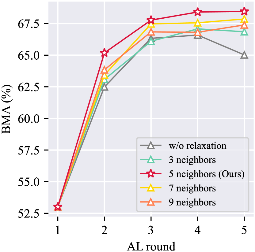
(a) Minimum neighbor size $n$

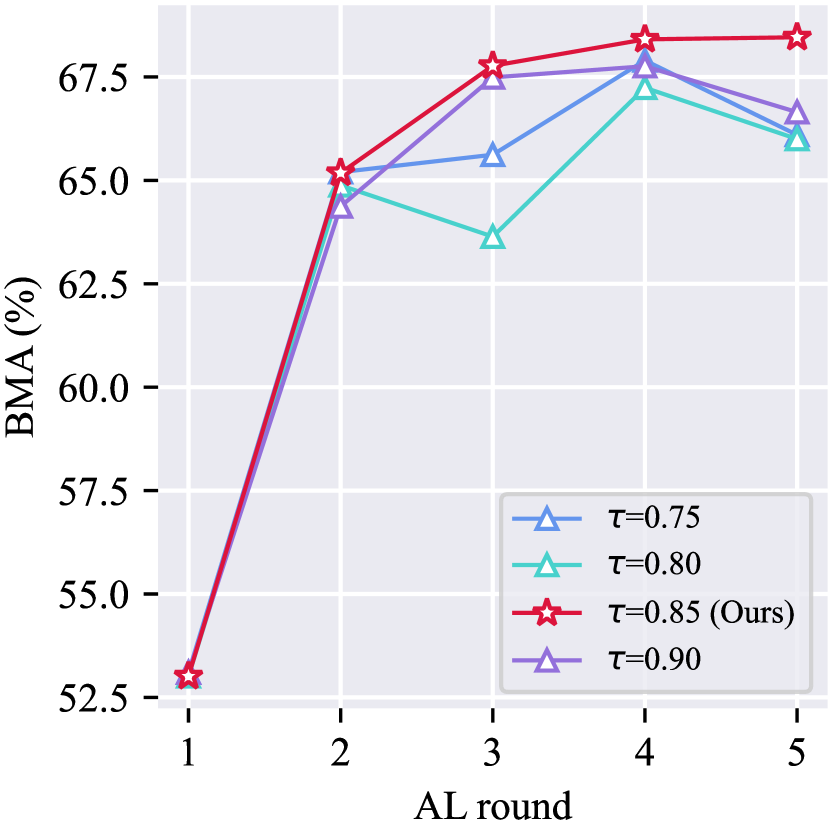
(b) Similarity threshold $\tau$

Figure 5: Ablation study of diversity relaxation on Fed-ISIC.

Effect of evidential model training

We performed experiments to compare the evidential loss against cross-entropy loss (CE) on the Fed-ISIC dataset and against dice loss (Dice) on the Fed-Polyp dataset. The results are detailed in Table 3. As can be seen, training with evidential loss results in an average performance gain of $1.03\%$ on the Fed-ISIC dataset and $1.16\%$ on the Fed-Polyp datasets, respectively. This improvement can be primarily attributed to evidence regularization, demonstrating the efficacy of evidential model training. The ablation results on the other three datasets are available in Appendix B.3.

Table 3: Effect of loss function on Fed-ISIC and Fed-Polyp.

Dataset	Loss	Round
		2	3	4	5
Fed-ISIC	CE	$64.28_{\pm 1.64}$	$66.69_{\pm 0.95}$	$67.32_{\pm 1.16}$	$67.40_{\pm 0.22}$
	$\mathcal{L}(\boldsymbol{x},\boldsymbol{\theta}_{k})$	$\boldsymbol{65.18_{\pm 0.41}}$	$\boldsymbol{67.77_{\pm 1.31}}$	$\boldsymbol{68.41_{\pm 1.01}}$	$\boldsymbol{68.46_{\pm 0.37}}$
Fed-Polyp	Dice	$70.14_{\pm 0.10}$	$75.77_{\pm 0.67}$	$77.23_{\pm 0.21}$	$79.48_{\pm 0.62}$
	$\mathcal{L}(\boldsymbol{x},\boldsymbol{\theta}_{k})$	$\boldsymbol{72.06_{\pm 0.72}}$	$\boldsymbol{76.39_{\pm 0.66}}$	$\boldsymbol{78.62_{\pm 1.44}}$	$\boldsymbol{80.18_{\pm 0.10}}$

Effect of trade-off weight $\lambda$

We further conducted experiments on the Fed-ISIC dataset to determine the optimal setting for the hyperparameter $\lambda$, choosing from the candidate set $\{1e-3,\ 5e-3,\ 1e-2,\ 5e-2,\ 1e-1\}$, the results are detailed in Table 4. As can be seen, the best performance is achieved when $\lambda=1e-2$. The ablation results on the Fed-Polyp dataset are reported in Appendix B.3.

Table 4: Ablation study of trade-off weight $\lambda$ on Fed-ISIC.

$\lambda$	Round
	2	3	4	5
$1e-3$	$63.49_{\pm 3.00}$	$64.57_{\pm 2.70}$	$66.25_{\pm 1.17}$	$65.45_{\pm 1.06}$
$5e-3$	$63.10_{\pm 2.07}$	$65.79_{\pm 2.57}$	$66.00_{\pm 2.09}$	$66.48_{\pm 0.86}$
$1e-2$	$\boldsymbol{65.18_{\pm 0.41}}$	$\boldsymbol{67.77_{\pm 1.31}}$	$\boldsymbol{68.41_{\pm 1.01}}$	$\boldsymbol{68.46_{\pm 0.37}}$
$5e-2$	$62.12_{\pm 0.99}$	$67.21_{\pm 1.42}$	$66.92_{\pm 0.70}$	$66.90_{\pm 0.93}$
$1e-1$	$63.53_{\pm 2.03}$	$66.21_{\pm 0.35}$	$66.03_{\pm 2.34}$	$67.78_{\pm 1.17}$

Analysis of Dirichlet simplex

We analyze the Dirichlet simplex on a subset of the Fed-ISIC encompassing three classes. As illustrated in Fig. 6, when selecting samples with FEAL, the Dirichlet distribution becomes more concentrated at the simplex’s corner for unlabeled local data, indicating reduced epistemic uncertainty in the global model. This trend verifies the effectiveness of CES in addressing domain shifts. Additionally, starting with an identical set of labeled samples, we tracked the selection of samples in the second FAL round utilizing various FAL methods. The Dirichlet simplexes of different methods are visualized in Fig. 7. As can be seen, the Dirichlet distribution of the samples selected by FEAL demonstrates a broader spread across the simplex. This spread indicates that FEAL effectively models the global model’s knowledge of local data and prioritizes selecting samples characterized by high epistemic uncertainty. More details and results are available in Appendix B.3.

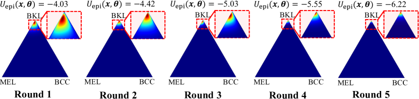
Figure 6: Visualization of the Dirichlet simplex for unlabeled samples across five FAL rounds using FEAL.

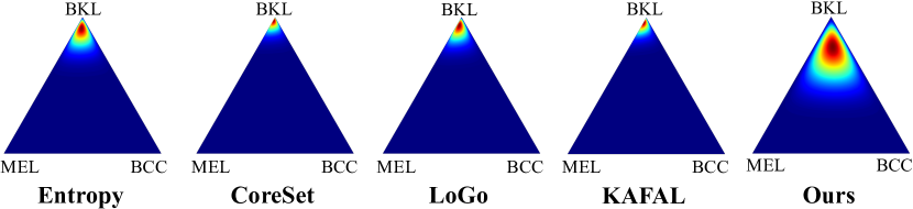
Figure 7: Visualization of the Dirichlet simplex for samples selected in the second FAL round using various sampling strategies.

5 Conclusion and Social Impact

To address the challenge of unreliable data assessment using the global model under domain shifts, we proposed a method FEAL, which places a Dirichlet prior over categorical probabilities to treat the prediction as a distribution over the probability simplex and leverages both aleatoric uncertainty and epistemic uncertainty to calibrate the uncertainty evaluation, enhancing the reliability of data assessment and incorporating diversity relaxation to maintain sample diversity. Extensive results verify the effectiveness. This work holds the potential to advance healthcare by preserving data privacy and facilitating collaborative research, ultimately leading to more accessible and effective patient care.

Supplementary Material

A Derivations

A.1 Dirichlet-based Evidential Model in FAL

In Dirichlet-based evidential models, given a sample $\boldsymbol{x}$ and a model $\boldsymbol{\theta}$, the categorical prediction $\boldsymbol{\rho}$ follows a Dirichlet distribution, denoted as $p(\boldsymbol{\rho}|\boldsymbol{x},\boldsymbol{\theta})\sim Dir(\boldsymbol{\rho}|\boldsymbol{\alpha})$. The probability density function of $\boldsymbol{\rho}$, conditioned on $\boldsymbol{x}$ and $\boldsymbol{\theta}$, is formulated as:

$$p(\boldsymbol{\rho}|\boldsymbol{x},\boldsymbol{\theta})=\left\{\begin{aligned} \frac{\Gamma(\sum_{c=1}^{C}\alpha_{c})}{\prod_{c=1}^{C}\Gamma(\alpha_{c})}\prod_{c=1}^{C}\boldsymbol{\rho}_{c}^{\alpha_{c}-1}&,(\boldsymbol{\rho}\in\Delta^{C})\\ 0\qquad\qquad&,(\text{otherwise})\end{aligned}\right.$$ (11)

where $\boldsymbol{\alpha}=\{\alpha_{1},\alpha_{2},\cdots,\alpha_{C}\}$ denotes the parameters of the Dirichlet distribution for sample $\boldsymbol{x}$, $\Gamma(\cdot)$ is the Gamma function, and $\Delta^{C}=\{\boldsymbol{\rho}|\sum_{c=1}^{C}\rho_{c}=1$ and $\forall\rho_{c},0<\rho_{c}<1\}$ is the $C$-dimensional unit simplex.

According to [36], the marginal distributions of Dirichlet are Beta distributions. Consequently, given $p(\boldsymbol{\rho}|\boldsymbol{x},\boldsymbol{\theta})\sim Dir(\boldsymbol{\rho}|\boldsymbol{\alpha})$, we have $p(\rho_{c}|\boldsymbol{x},\boldsymbol{\theta})\sim Beta(\rho_{c}|\alpha_{c},S-\alpha_{c})$, where $S=\sum_{c=1}^{C}\alpha_{c}$ represents the Dirichlet strength. The probability density function of $\rho_{c}$, given $\boldsymbol{x}$ and $\boldsymbol{\theta}$, is formulated as:

$$\small p(\rho_{c}|\boldsymbol{x},\boldsymbol{\theta})=\frac{1}{\mathcal{B}(\alpha_{c},S-\alpha_{c})}\rho_{c}^{\alpha_{c}-1}(1-\rho_{c})^{S-\alpha_{c}-1},$$ (12)

where $\mathcal{B(\cdot,\cdot)}$ is the Beta function and $\mathcal{B}(\alpha_{c},S-\alpha_{c})=\frac{\Gamma(\alpha_{c})\cdot\Gamma(S-\alpha_{c})}{\Gamma(\alpha_{c}+S-\alpha_{c})}=\frac{\Gamma(\alpha_{c})\cdot\Gamma(S-\alpha_{c})}{\Gamma(S)}$.

Combining Eq. 11 and Eq. 12, the posterior probability for class $c$ can be obtained as:

$$P(y=c|\boldsymbol{x},\boldsymbol{\theta}) =\int p(y=c|\boldsymbol{\rho})\cdot p(\boldsymbol{\rho}|\boldsymbol{x},\boldsymbol{\theta})\ \text{d}\boldsymbol{\rho}$$ (13)

$$=\int\rho_{c}\cdot p(\boldsymbol{\rho}|\boldsymbol{x},\boldsymbol{\theta})\ \text{d}\boldsymbol{\rho}$$

$$=\int\rho_{c}\cdot p(\rho_{c}|\boldsymbol{x},\boldsymbol{\theta})\ \text{d}\rho_{c}$$

$$=\frac{\mathcal{B}(\alpha_{c}+1,S-\alpha_{c})}{\mathcal{B}(\alpha_{c},S-\alpha_{c})}\int\frac{\rho_{c}^{\alpha_{c}}(1-\rho_{c})^{S-\alpha_{c}-1}}{\mathcal{B}(\alpha_{c}+1,S-\alpha_{c})}\ \text{d}\rho_{c}$$

$$=\frac{\mathcal{B}(\alpha_{c}+1,S-\alpha_{c})}{\mathcal{B}(\alpha_{c},S-\alpha_{c})}$$

$$=\frac{\Gamma(\alpha_{c}+1)\cdot\Gamma(S)}{\Gamma(S+1)\cdot\Gamma(\alpha_{c})}$$

$$=\frac{\alpha_{c}}{S}.$$

The Dirichlet distribution parameter $\boldsymbol{\alpha}$ is closely linked to the evidence $\boldsymbol{e}$ which reflects the support for the model prediction on the given sample $\boldsymbol{x}$. The parameter $\boldsymbol{\alpha}$ is formulated as:

$$\small\boldsymbol{\alpha}=\boldsymbol{e}+1=\mathcal{A}(f(\boldsymbol{x},\boldsymbol{\theta}))+1,$$ (14)

where $f(\boldsymbol{x},\boldsymbol{\theta})$ denotes the output logits of model $\boldsymbol{\theta}$ for sample $\boldsymbol{x}$, and $\mathcal{A}(\cdot)$ is a non-negative activation function to transform the logits $f(\boldsymbol{x},\boldsymbol{\theta})$ into evidence $\boldsymbol{e}$. There are several common activation functions $\mathcal{A}(\cdot)$ include: $ReLU(\cdot)=\max(0,\cdot)$, $SoftPlus(\cdot)=\log(1+\exp(\cdot))$ and $\exp(\cdot)$. In our study, $ReLU(\cdot)$ was employed as the non-negative activation function.

A.2 Calibrated Evidential Sampling

Aleatoric uncertainty

Given a sample $\boldsymbol{x}$ and the global model $\boldsymbol{\theta}$, the expected entropy of all possible predictions is utilized to depict the aleatoric uncertainty. The aleatoric uncertainty of sample $\boldsymbol{x}$ in model $\boldsymbol{\theta}$ is formulated as:

$$U_{\text{ale}}(\boldsymbol{x},\boldsymbol{\theta}) =\mathbb{E}_{p(\boldsymbol{\rho}|\boldsymbol{x},\boldsymbol{\theta})}[\mathcal{H}[P(y|\boldsymbol{\rho})]]$$ (15)

$$=-\sum_{c=1}^{C}\mathbb{E}_{p(\boldsymbol{\rho}|\boldsymbol{x},\boldsymbol{\theta})}[\rho_{c}\cdot\log\rho_{c}]$$

$$=-\sum_{c=1}^{C}\mathbb{E}_{p(\rho_{c}|\boldsymbol{x},\boldsymbol{\theta})}[\rho_{c}\cdot\log\rho_{c}]$$

$$=-\sum_{c=1}^{C}\int\log(\rho_{c})\cdot\frac{\rho_{c}^{\alpha_{c}}(1-\rho_{c})^{S-\alpha_{c}-1}}{\mathcal{B}(\alpha_{c},S-\alpha_{c})}\ \text{d}\rho_{c}$$

$$=-\sum_{c=1}^{C}\frac{\mathcal{B}(\alpha_{c}+1,S-\alpha_{c})}{\mathcal{B}(\alpha_{c},S-\alpha_{c})}\int\log(\rho_{c})\frac{\rho_{c}^{\alpha_{c}}(1-\rho_{c})^{S-\alpha_{c}-1}}{\mathcal{B}(\alpha_{c}+1,S-\alpha_{c})}\ \text{d}\rho_{c}$$

$$=-\sum_{c=1}^{C}\frac{\Gamma(\alpha_{c}+1)\cdot\Gamma(S)}{\Gamma(S+1)\cdot\Gamma(\alpha_{c})}\mathbb{E}_{\rho_{c}\sim Beta(\rho_{c}|\alpha_{c}+1,S-\alpha_{c})}[\log\rho_{c}]$$

$$=\sum_{c=1}^{C}\frac{\alpha_{c}}{S}\cdot[\psi(S+1)-\psi(\alpha_{c}+1)],$$

where $\mathcal{H}(\cdot)$ denotes the Shannon entropy [47] and $\psi(\cdot)$ represents the digamma function. The aleatoric uncertainty of sample $\boldsymbol{x}$ in local model $\boldsymbol{\theta}_{k}$ is calculated as $U_{\text{ale}}(\boldsymbol{x},\boldsymbol{\theta}_{k})$ according to Eq. 15.

Epistemic uncertainty

The differential entropy of a Dirichlet distribution is employed to quantify the inherent randomness in categorical distributions. This metric is beneficial in depicting epistemic uncertainty, which arises due to the global model’s lack of knowledge, often caused by domain shifts. Given a sample $\boldsymbol{x}$ and the global model $\boldsymbol{\theta}$, the epistemic uncertainty is defined as:

$$U_{\text{epi}}(\boldsymbol{x},\boldsymbol{\theta}) =\mathcal{H}[p(\boldsymbol{\rho}|\boldsymbol{x},\boldsymbol{\theta})]$$ (16)

$$=-\int p(\boldsymbol{\rho}|\boldsymbol{x},\boldsymbol{\theta})\log p(\boldsymbol{\rho}|\boldsymbol{x},\boldsymbol{\theta})\ \text{d}\boldsymbol{\rho}$$

$$=\sum_{c=1}^{C}\log\frac{\Gamma(\alpha_{c})}{\Gamma(S)}-\sum_{c=1}^{C}(\alpha_{c}-1)\cdot[\psi(\alpha_{c})-\psi(S)].$$

A.3 Evidential Model Training

Task loss for classification

We employ the Bayes risk of cross-entropy loss as the task loss for classification. Given an input pair $(\boldsymbol{x},\boldsymbol{y})$, the task loss for classification is:

$$\mathcal{L}_{\text{task}}(\boldsymbol{x},\boldsymbol{\theta}_{k},\boldsymbol{y}) =\mathbb{E}_{p(\boldsymbol{\rho}|\boldsymbol{x},\boldsymbol{\theta}_{k})}[\mathcal{L}_{CE}(\boldsymbol{x},\boldsymbol{\theta}_{k},\boldsymbol{y})]$$ (17)

$$=\int[\sum_{c=1}^{C}-y_{c}\log(\rho_{c})]\cdot p(\boldsymbol{\rho}|\boldsymbol{x},\boldsymbol{\theta}_{k})\ \text{d}\boldsymbol{\rho}$$

$$=-\sum_{c=1}^{C}y_{c}\int\log(\rho_{c})\cdot p(\rho_{c}|\boldsymbol{x},\boldsymbol{\theta}_{k})\ \text{d}\rho_{c}$$

$$=-\sum_{c=1}^{C}y_{c}\cdot\mathbb{E}_{\rho_{c}\sim Beta(\rho_{c}|\alpha_{c},S-\alpha_{c})}[\log\rho_{c}]$$

$$=\sum_{c=1}^{C}y_{c}\cdot[\psi(S)-\psi(\alpha_{c})].$$

Task loss for segmentation

We leverage the Bayes risk of Dice loss as the task loss for segmentation. Given an input pair $(\boldsymbol{x},\boldsymbol{y})$, the task loss for segmentation is:

$$\mathcal{L}_{\text{task}}(\boldsymbol{x},\boldsymbol{\theta}_{k},\boldsymbol{y}) =\mathbb{E}_{p(\boldsymbol{\rho}|\boldsymbol{x},\boldsymbol{\theta}_{k})}[\mathcal{L}_{Dice}(\boldsymbol{x},\boldsymbol{\theta}_{k},\boldsymbol{y})]$$ (18)

$$=\mathbb{E}_{p(\boldsymbol{\rho}|\boldsymbol{x},\boldsymbol{\theta}_{k})}[1-\frac{2}{C}\sum_{c=1}^{C}\frac{\sum_{m=1}^{M}y_{mc}\cdot\rho_{mc}}{\sum_{m=1}^{M}(y_{mc}^{2}+\rho_{mc}^{2})}]$$

$$=1-\frac{2}{C}\sum_{c=1}^{C}\frac{\sum_{m=1}^{M}y_{mc}\cdot\mathbb{E}[\rho_{mc}]}{\sum_{m=1}^{M}(y_{mc}^{2}+\mathbb{E}[\rho_{mc}^{2}])},$$

where $\boldsymbol{x}$ is comprised of $M$ pixels. By using the following equation:

$$\small\mathbb{E}[\rho_{mc}^{2}]=\mathbb{E}[\rho_{mc}]^{2}+\text{Var}(\rho_{mc}),$$ (19)

Eq. 18 can be updated to:

$$\small\mathcal{L}_{\text{task}}(\boldsymbol{x},\boldsymbol{\theta}_{k},\boldsymbol{y})=1-\frac{2}{C}\sum_{c=1}^{C}\frac{\sum_{m=1}^{M}y_{mc}\cdot\overline{\rho}_{mc}}{\sum_{m=1}^{M}[y_{mc}^{2}+\overline{\rho}_{mc}^{2}+\frac{\overline{\rho}_{mc}(1-\overline{\rho}_{mc})}{S_{m}+1}]}.$$ (20)

B Experiments

Dataset	Data source	# Train	# Test	Resolution
Fed-ISIC	Client 1: BCN [38]	9,930	2,483	$224\times 224$
	Client 2: HAM_vidir_molemax [38]	3,163	791
	Client 3: HAM_vidir_modern [38]	2,691	672
	Client 4: HAM_rosendahl [38]	1,807	452
Fed-Camelyon	Client 1: Camelyon17 [3]	47,548	11,888	$96\times 96$
	Client 2: Camelyon17 [3]	27,923	6,981
	Client 3: Camelyon17 [3]	68,043	17,011
	Client 4: Camelyon17 [3]	103,870	25,968
	Client 5: Camelyon17 [3]	117,377	29,345
Fed-Polyp	Client 1: Kvasir [30]	800	200	$384\times 384$
	Client 2: ETIS [48]	157	39
	Client 3: ColonDB [50]	304	75
	Client 4: ClinicDB [4]	490	122
Fed-Prostate	Client 1: BIDMC [30]	225	36	$320\times 320$
	Client 2: BMC [5]	306	78
	Client 3: HK [30]	134	24
	Client 4: I2CVB [26]	387	81
	Client 5: RUNMC [5]	337	84
	Client 6: UCL [30]	152	23
Fed-Fundus	Client 1: Drishti-GS [49]	81	20	$320\times 320$
	Client 2: RIM-ONE-r3 [11]	128	31
	Client 3: REFUGE [39]	320	80
	Client 4: REFUGE [39]	320	80

Table 5: Details of multi-center datasets utilized in our study.

B.1 Experimental Settings

Datasets

We verified the effectiveness of FEAL across five real-world medical image datasets, two for classification and three for segmentation. Detailed information, including the data source, the number of samples, and the resolution of each sample, is summarized in Table 5. Note that the Camelyon17 [3] dataset comprises five distinct data sources with varying stains; we decomposed them in the FAL framework. Similarly, the REFUGE [39] dataset contains data from two separate sources, each of which was treated as an individual client in federated scenarios.

Evaluation metrics

For classification, we utilized the Balanced Multi-class Accuracy (BMA) for skin lesion classification [8] and measured accuracy (ACC) for breast cancer histology classification. In the context of segmentation, we used the Dice score and the 95% Hausdorff Distance (HD95) to assess segmentation results.

Implemental details

We conducted $R=5$ rounds of FAL involving federated model training and data annotation. During model training, we followed the previous work [57, 19, 55] to utilize EfficientNet-B0 [51] for the Fed-ISIC dataset, DenseNet-121 [15] for the Fed-Camelyon dataset, and U-Net [43] for segmentation datasets. Notably, both EfficientNet-B0 and DenseNet-121 were pre-trained on ImageNet [9]. In FEAL, we employed the $ReLU(\cdot)$ activation as the non-negative activation function $\mathcal{A}(\cdot)$ for both global and local models. We trained local models using the Adam optimizer [22] with a learning rate of $5e-4$. The weight decay was set to $5e-4$ for the Fed-ISIC dataset and $1e-5$ for the other four datasets. In terms of communication, we employed the FedAvg algorithm [23], with all clients participating in each communication round. We conducted $T=100$ rounds of communication to attain a robust global model. Regarding data annotation, we followed the previous work [21, 6] to a uniform annotation budget $B_{k}$ across all local clients $k$. Specifically, annotation budget $B_{k}$ is allocated based on the size of each dataset. $B_{k}$ was set to $500$ for the Fed-ISIC and Fed-Camelyon datasets, $20$ for both Fed-Prostate and Fed-Fundus datasets, and $50$ for the Fed-Polyp dataset. Furthermore, to account for the different sizes of datasets among local clients, we established a maximum annotation ratio of $85\%$. The clients whose number of labeled samples achieves the threshold ceased further data annotation. All the experiments were conducted three times using different random seeds, and the average results were reported.

Comparison methods

We compared FEAL with eight state-of-the-art FAL approaches, including random sampling (Random), entropy-based sampling (Entropy) [47], TOD [16], Gradnorm [56], CoreSet [44], BADGE [2], LoGo [21], and KAFAL [6]. The first six methods are designed for standard active learning, whereas LoGo and KAFAL are specifically tailored for federated scenarios. For a comprehensive comparison, we implemented the first six sampling strategies in three distinct manners: (1) utilizing the global model for data evaluation, (2) employing the local model for data evaluation, and (3) integrating an ensemble technique that harnesses both global and local models for evaluation. The details of comparison methods and ensemble techniques are summarized as follows.

• Random: Randomly select $B_{k}$ unlabeled samples for local client $k$ in each FAL round.

• Entropy [47]: Entropy is a conventional uncertainty-based AL method, which selects the top-$B_{k}$ unlabeled samples with the highest entropy scores in model predictions. Besides using the global or local model individually, a straightforward ensemble approach aggregating entropy scores in both models is also implemented.

• TOD [16]: TOD leverages the temporal output discrepancy to quantify the uncertainty of unlabeled samples. It selects the top-$B_{k}$ unlabeled samples with the highest cyclic output discrepancy (COD) scores. In our implementation, we incorporated an additional ensemble technique [21], fine-tuning, into TOD. Specifically, local client $k$ downloads the global model $\boldsymbol{\theta}^{r}$ and fine-tunes it with the available labeled samples. Subsequently, local client $k$ employs both the fine-tuned global model and its historical local model $\boldsymbol{\theta}_{k}^{r-1}$ to compute the COD score, thereby integrating insights from both global and local models for more effective sampling.

• Gradnorm [56]: Gradnorm initially computes the pseudo loss through pseudo labels or entropy scores from model predictions, which is then backpropagated to determine the gradient norm across all model parameters. This gradient norm serves as a measure of data uncertainty to evaluate the potential value of each unlabeled sample. To leverage the knowledge of both global and local models, we aggregated the gradient norm from both models for a more comprehensive evaluation.

• CoreSet [44]: CoreSet, a diversity-based sampling strategy, selects $B_{K}$ unlabeled samples whose feature embeddings exhibit the greatest dissimilarity to labeled samples. For the ensemble approach, we computed the average feature embedding from both global and local models for each sample. Subsequently, CoreSet was applied based on the interpolated feature embedding.

• BADGE [2]: BADGE is a hybrid sampling strategy that simultaneously considers uncertainty and diversity metrics. It begins by extracting gradient embeddings of unlabeled samples to ensure uncertainty. Following this, it employs $k$-means clustering on these gradient embeddings to maintain a diverse selection of samples.

• LoGo [21]: LoGo is designed to address class-imbalance issues in FAL. It first performed $k$-means clustering with gradient embeddings extracted from the local model. Then it applied cluster-wise sampling to select the most uncertain sample within each cluster, identified by the highest entropy score in the global model.

• KAFAL [6]: KAFAL is another sampling strategy tailored for FAL with class imbalance. It employs a knowledge-specialized KL divergence, calculated between the global and local models, to quantify the informativeness of unlabeled samples for both models. For fair comparisons in our study, we implemented KAFAL by exclusively using the supervised loss component.

B.2 Results

Table 6: Comparison results ($\text{mean}_{\pm\text{std}}$) on medical image datasets for classification. We evaluated the balanced multi-class accuracy (BMA) for Fed-ISIC and the accuracy for Fed-Camelyon and presented the mean result and standard deviation of three random seeds. Red and blue highlights the Top-1 and Top-2 results, respectively.

Model	Method	Fed-ISIC (%)				Fed-Camelyon (%)
		R2	R3	R4	R5	R2	R3	R4	R5
-	Random	$61.59_{\pm 1.45}$	$64.90_{\pm 1.53}$	$65.53_{\pm 1.31}$	$64.99_{\pm 1.43}$	$94.82_{\pm 0.30}$	$95.40_{\pm 0.24}$	$96.02_{\pm 0.12}$	$96.34_{\pm 0.07}$
$G$	Entropy [47]	$61.82_{\pm 1.38}$	$65.74_{\pm 1.62}$	$65.99_{\pm 0.35}$	$64.44_{\pm 1.21}$	$94.91_{\pm 0.54}$	$95.98_{\pm 0.14}$	$96.53_{\pm 0.16}$	$96.84_{\pm 0.14}$
	TOD [16]	$56.63_{\pm 3.05}$	$64.13_{\pm 3.50}$	$65.32_{\pm 1.10}$	$64.54_{\pm 0.76}$	$93.48_{\pm 1.23}$	$95.47_{\pm 0.54}$	$96.41_{\pm 0.31}$	$96.81_{\pm 0.16}$
	Gradnorm [56]	$63.20_{\pm 0.49}$	$65.72_{\pm 1.29}$	$65.31_{\pm 2.03}$	$64.61_{\pm 0.76}$	$94.10_{\pm 0.18}$	$94.95_{\pm 0.23}$	$95.27_{\pm 0.15}$	$95.73_{\pm 0.18}$
	CoreSet [44]	$62.19_{\pm 1.57}$	$66.73_{\pm 0.49}$	$66.33_{\pm 0.30}$	$65.62_{\pm 1.09}$	$93.89_{\pm 0.53}$	$94.15_{\pm 0.26}$	$95.14_{\pm 0.35}$	$96.04_{\pm 0.18}$
	BADGE [2]	$62.26_{\pm 1.74}$	$64.98_{\pm 1.56}$	$65.46_{\pm 1.94}$	$64.39_{\pm 0.63}$	$94.87_{\pm 0.38}$	$95.55_{\pm 0.19}$	$96.07_{\pm 0.16}$	$96.29_{\pm 0.25}$
$L$	Entropy [47]	$62.61_{\pm 3.39}$	$64.95_{\pm 1.87}$	$66.93_{\pm 1.44}$	$65.76_{\pm 2.34}$	$95.07_{\pm 0.24}$	$96.05_{\pm 0.03}$	$96.68_{\pm 0.07}$	$96.73_{\pm 0.12}$
	TOD [16]	$58.52_{\pm 2.89}$	$65.11_{\pm 2.04}$	$64.88_{\pm 2.00}$	$64.81_{\pm 3.11}$	$93.79_{\pm 1.18}$	$95.29_{\pm 0.47}$	$96.46_{\pm 0.34}$	$96.83_{\pm 0.11}$
	Gradnorm [56]	$62.38_{\pm 1.90}$	$64.96_{\pm 3.21}$	$65.85_{\pm 2.79}$	$64.39_{\pm 1.44}$	$94.22_{\pm 0.38}$	$94.98_{\pm 0.39}$	$95.37_{\pm 0.54}$	$95.92_{\pm 0.26}$
	CoreSet [44]	$63.16_{\pm 0.70}$	$66.84_{\pm 0.49}$	$66.43_{\pm 0.89}$	$66.40_{\pm 0.36}$	$93.92_{\pm 0.40}$	$94.12_{\pm 0.24}$	$95.24_{\pm 0.34}$	$95.87_{\pm 0.17}$
	BADGE [2]	$63.12_{\pm 0.72}$	$65.54_{\pm 1.47}$	$65.41_{\pm 1.77}$	$64.80_{\pm 2.39}$	$95.09_{\pm 0.23}$	$95.73_{\pm 0.27}$	$96.14_{\pm 0.21}$	$96.50_{\pm 0.05}$
$E$	Entropy [47]	$63.21_{\pm 0.59}$	$64.86_{\pm 1.09}$	$66.35_{\pm 0.14}$	$65.57_{\pm 1.92}$	$95.03_{\pm 0.01}$	$96.08_{\pm 0.23}$	$96.52_{\pm 0.20}$	$96.88_{\pm 0.18}$
	TOD [16]	$58.10_{\pm 1.95}$	$66.56_{\pm 0.36}$	$66.26_{\pm 1.22}$	$65.51_{\pm 0.75}$	$93.17_{\pm 0.87}$	$95.27_{\pm 0.07}$	$96.07_{\pm 0.09}$	$96.50_{\pm 0.12}$
	Gradnorm [56]	$63.23_{\pm 1.25}$	$66.14_{\pm 1.51}$	$67.02_{\pm 1.00}$	$66.52_{\pm 0.75}$	$94.40_{\pm 0.06}$	$94.85_{\pm 0.21}$	$95.64_{\pm 0.04}$	$95.89_{\pm 0.13}$
	CoreSet [44]	$62.53_{\pm 1.50}$	$65.91_{\pm 0.78}$	$66.61_{\pm 0.20}$	$66.84_{\pm 0.21}$	$93.90_{\pm 0.25}$	$93.95_{\pm 0.31}$	$94.94_{\pm 0.09}$	$95.85_{\pm 0.13}$
	BADGE [2]	$59.45_{\pm 0.67}$	$64.27_{\pm 0.74}$	$66.73_{\pm 0.46}$	$64.71_{\pm 1.07}$	$94.97_{\pm 0.41}$	$95.62_{\pm 0.11}$	$96.25_{\pm 0.12}$	$96.37_{\pm 0.10}$
	LoGo [21]	$62.36_{\pm 2.30}$	$66.43_{\pm 0.69}$	$66.12_{\pm 2.64}$	$66.26_{\pm 0.50}$	$94.98_{\pm 0.07}$	$95.60_{\pm 0.15}$	$96.20_{\pm 0.26}$	$96.51_{\pm 0.05}$
	KAFAL [6]	$62.34_{\pm 0.32}$	$65.36_{\pm 1.15}$	$66.26_{\pm 1.22}$	$66.24_{\pm 1.31}$	$95.06_{\pm 0.17}$	$96.08_{\pm 0.07}$	$96.76_{\pm 0.11}$	$96.92_{\pm 0.04}$
	Ours	$65.18_{\pm 0.41}$	$67.77_{\pm 1.31}$	$68.41_{\pm 1.01}$	$68.46_{\pm 0.37}$	$95.79_{\pm 0.68}$	$96.54_{\pm 0.40}$	$97.04_{\pm 0.28}$	$97.29_{\pm 0.35}$

Image classification

Table 6 summarizes the quantitative results of image classification. From the second to the fifth FAL rounds, FEAL demonstrates superior performance over the second-best method, achieving margins of $1.95\%$, $0.92\%$, $1.39\%$, and $1.62\%$ on the Fed-ISIC dataset, respectively. Additionally, on the Fed-Camelyon dataset, FEAL maintains a consistent performance advantage, surpassing the second-best method by margins of $0.69\%$, $0.46\%$, $0.32\%$, and $0.37\%$ in these rounds.

Image segmentaion

The mean result and standard deviation of Dice and HD95 metrics for the Fed-Polyp, Fed-Prostate, and Fed-Fundus datasets are illustrated in Fig. 8, Fig. 9, and Fig. 10. As can be seen, FEAL demonstrates superior performance on three multi-center segmentation datasets, as evidenced by its enhanced Dice scores and reduced HD95 metrics.

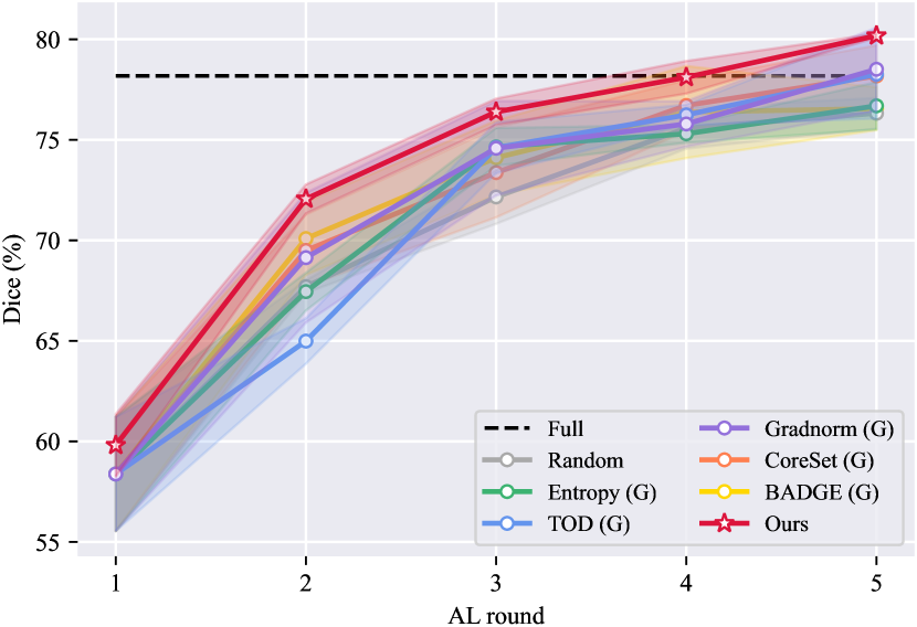
(a) Dice of Fed-Polyp (global model)

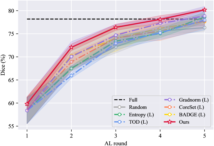
(b) Dice of Fed-Polyp (local model)

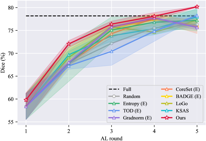
(c) Dice of Fed-Polyp (global and local models)

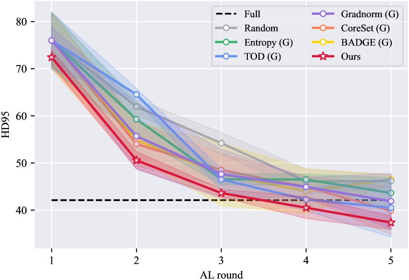
(d) HD95 of Fed-Polyp (global model)

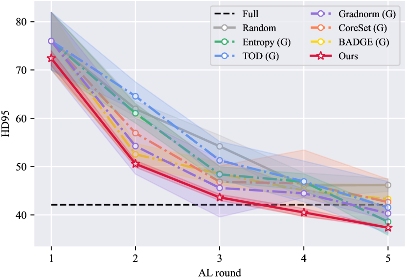
(e) HD95 of Fed-Polyp (local model)

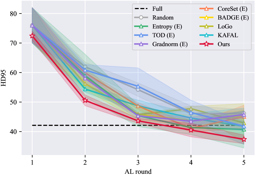
(f) HD95 of Fed-Polyp (global and local models)

Figure 8: Comparison results on the Fed-Polyp dataset.

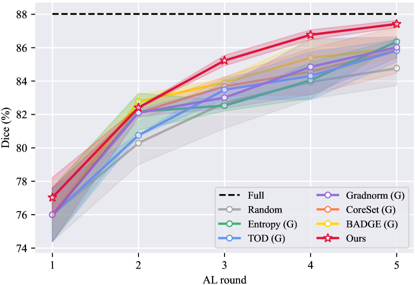
(a) Dice of Fed-Prostate (global model)

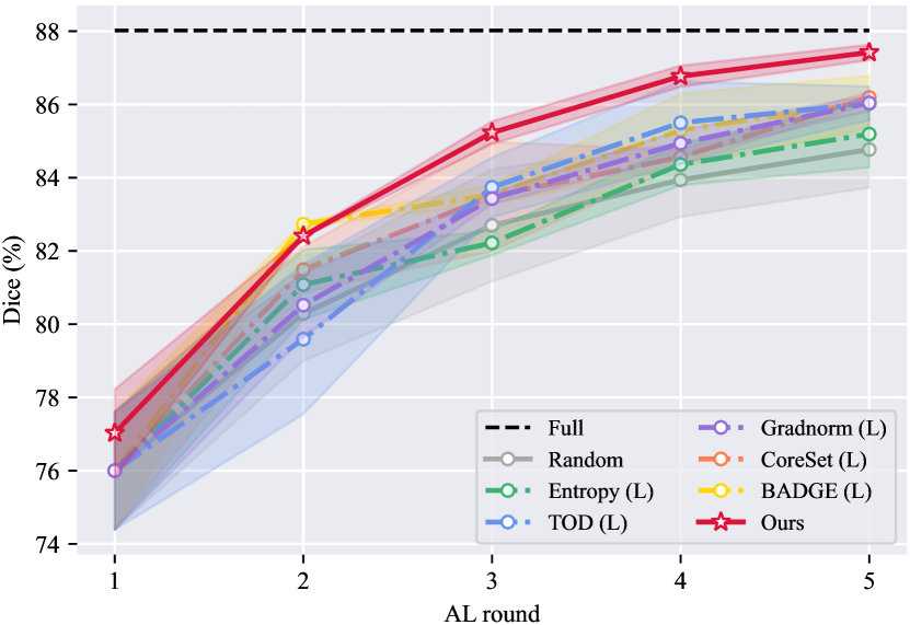
(b) Dice of Fed-Prostate (local model)

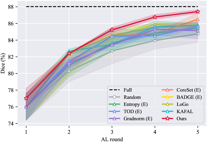
(c) Dice of Fed-Prostate (global and local models)

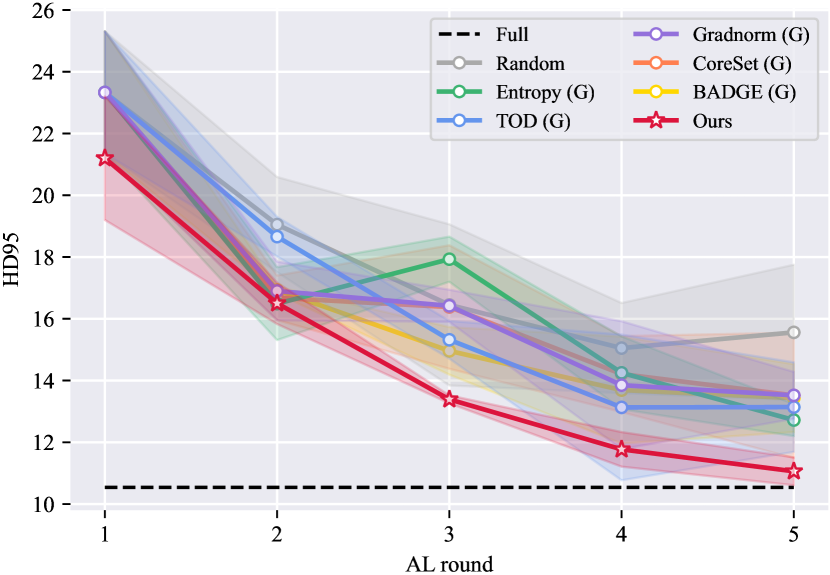
(d) HD95 of Fed-Prostate (global model)

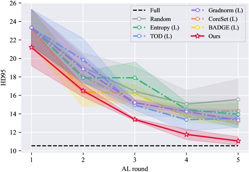
(e) HD95 of Fed-Prostate (local model)

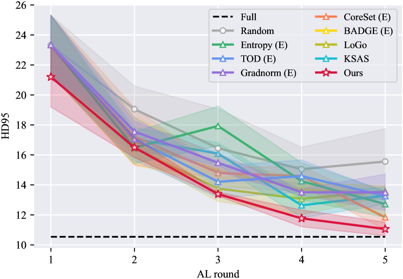
(f) HD95 of Fed-Prostate (global and local models)

Figure 9: Comparison results on the Fed-Prostate dataset.

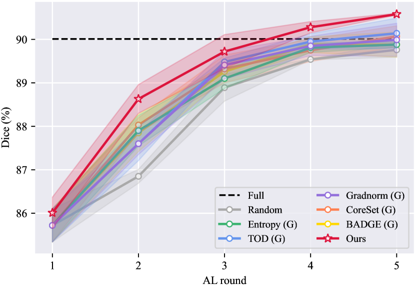
(a) Dice of Fed-Fundus (global model)

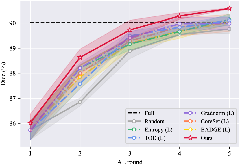
(b) Dice of Fed-Fundus (local model)

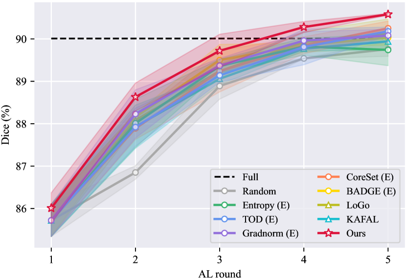
(c) Dice of Fed-Fundus (global and local models)

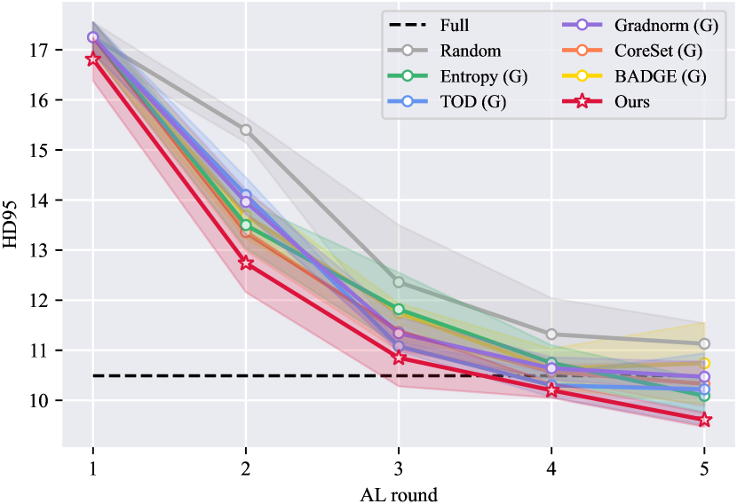
(d) HD95 of Fed-Fundus (global model)

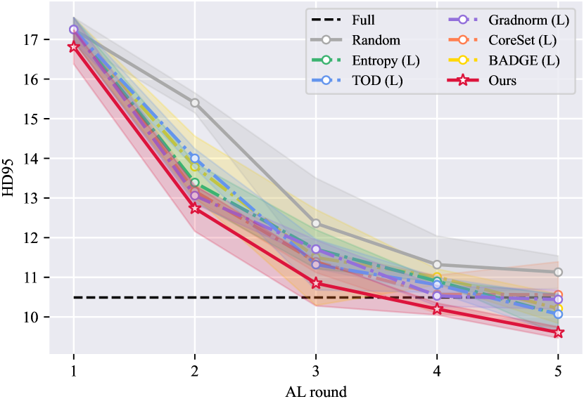
(e) HD95 of Fed-Fundus (local model)

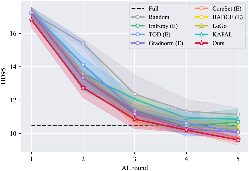
(f) HD95 of Fed-Fundus (global and local models)

Figure 10: Comparison results on the Fed-Fundus dataset.

B.3 Discussions

Effect of uncertainty calibration

In addition to the ablation study conducted on the Fed-ISIC dataset for classification, we expanded our analysis to include the Fed-Polyp dataset, specifically examining the impact of uncertainty calibration in segmentation tasks. The results, including the average Dice score and the corresponding standard deviation, are summarized in Table 7.

Table 7: Ablation study of uncertainty calibration on Fed-Polyp.

Strategy			Round
$U_{\text{epi}}(\cdot,\boldsymbol{\theta})$	$U_{\text{ale}}(\cdot,\boldsymbol{\theta})$	$U_{\text{ale}}(\cdot,\boldsymbol{\theta}_{k})$	2	3	4	5
-	✓	-	$68.61_{\pm 0.48}$	$73.12_{\pm 2.38}$	$75.19_{\pm 1.10}$	$78.00_{\pm 1.14}$
-	-	✓	$69.13_{\pm 1.15}$	$75.19_{\pm 1.29}$	$77.85_{\pm 1.20}$	$78.12_{\pm 1.29}$
-	✓	✓	$66.89_{\pm 3.41}$	$74.48_{\pm 1.00}$	$76.56_{\pm 1.49}$	$76.86_{\pm 0.43}$
✓	-	-	$70.61_{\pm 4.22}$	$74.45_{\pm 2.29}$	$75.07_{\pm 2.42}$	$78.25_{\pm 1.29}$
✓	✓	-	$69.41_{\pm 2.17}$	$75.18_{\pm 2.48}$	$74.66_{\pm 0.87}$	$78.91_{\pm 1.04}$
✓	-	✓	$69.29_{\pm 2.51}$	$75.93_{\pm 1.41}$	$76.74_{\pm 1.08}$	$78.28_{\pm 0.67}$
✓	✓	✓	$\boldsymbol{72.06_{\pm 0.72}}$	$\boldsymbol{76.39_{\pm 0.66}}$	$\boldsymbol{78.62_{\pm 0.81}}$	$\boldsymbol{80.18_{\pm 0.10}}$

Effect of diversity relaxation

Besides carrying out the ablation study on the Fed-ISIC dataset, we further conducted experiments on the Fed-Polyp dataset to investigate the impact of diversity relaxation. As illustrated in Fig. 11, the optimal performance was attained when setting the minimum neighbor size to $n=10$ and the cosine similarity threshold to $\tau=0.90$ on the Fed-Polyp dataset.

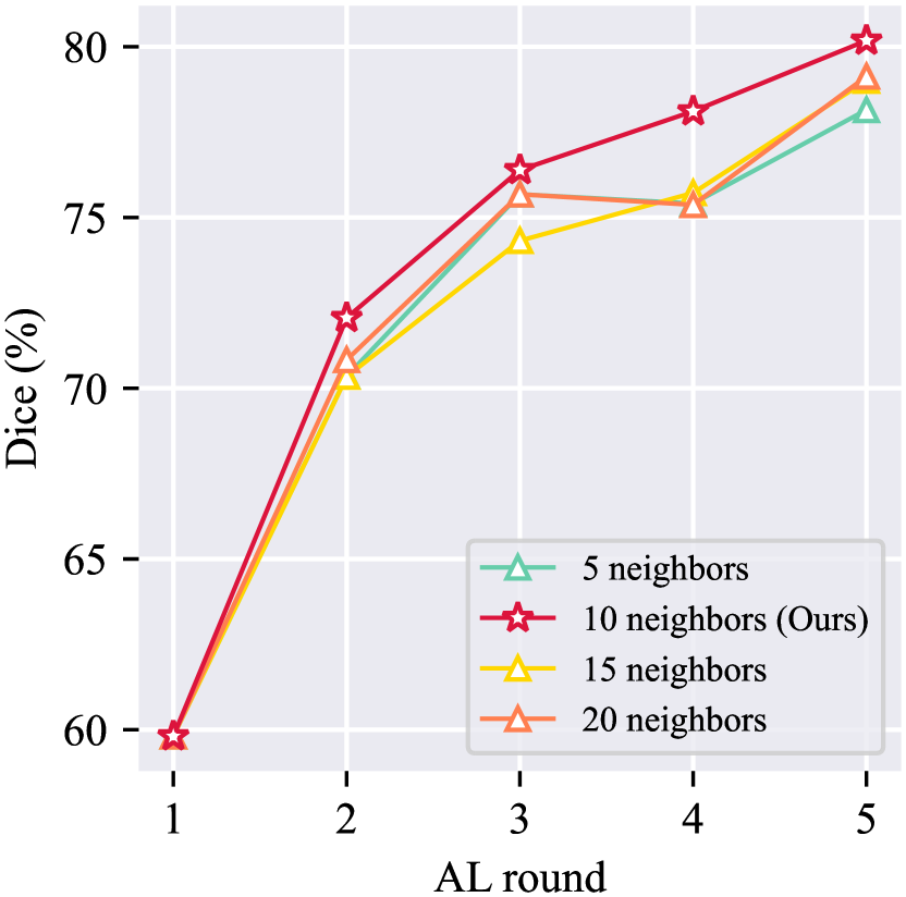
(a) Minimum neighbor size $n$.

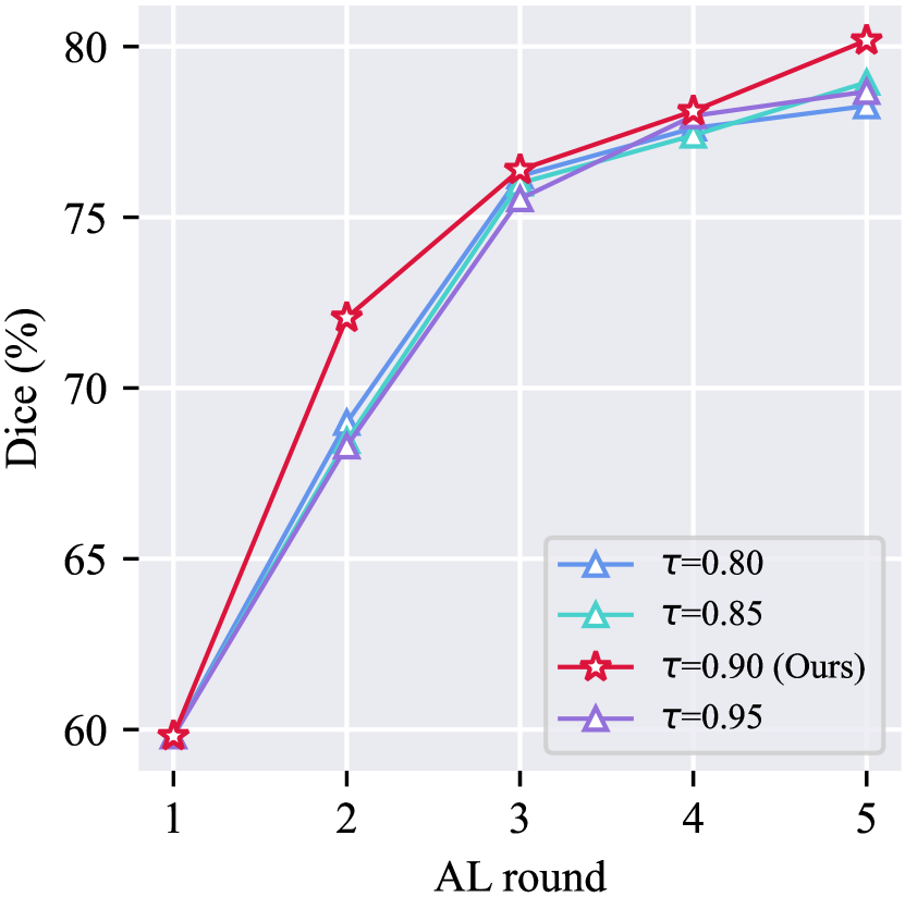
(b) Similarity threshold $\tau$.

Figure 11: Ablation study of diversity relaxation on Fed-Polyp.

Effect of evidential model training

We conducted experiments to compare the evidential loss against the cross-entropy loss (CE) on two classification datasets and against dice loss (Dice) on three segmentation datasets. As summarized in Table 8, the proposed evidential model training yields an average performance gain of $1.03\%$ on the Fed-ISIC dataset, $0.29\%$ on the Fed-Camelyon dataset, $1.16\%$ on the Fed-Polyp dataset, $1.17\%$ on the Fed-Prostate dataset, and $0.36\%$ on the Fed-Fundus dataset.

Table 8: Effects of loss function on five datasets.

Dataset	Loss	Round
		2	3	4	5
Fed-ISIC	CE	$64.28_{\pm 1.64}$	$66.69_{\pm 0.95}$	$67.32_{\pm 1.16}$	$67.40_{\pm 0.22}$
	$\mathcal{L}(\boldsymbol{x},\boldsymbol{\theta}_{k})$	$\boldsymbol{65.18_{\pm 0.41}}$	$\boldsymbol{67.77_{\pm 1.31}}$	$\boldsymbol{68.41_{\pm 1.01}}$	$\boldsymbol{68.46_{\pm 0.37}}$
Fed-Camelyon	CE	$95.24_{\pm 0.03}$	$96.21_{\pm 0.04}$	$96.80_{\pm 0.07}$	$97.26_{\pm 0.06}$
	$\mathcal{L}(\boldsymbol{x},\boldsymbol{\theta}_{k})$	$\boldsymbol{95.79_{\pm 0.17}}$	$\boldsymbol{96.54_{\pm 0.08}}$	$\boldsymbol{97.04_{\pm 0.02}}$	$\boldsymbol{97.29_{\pm 0.02}}$
Fed-Polyp	Dice	$70.14_{\pm 0.10}$	$75.77_{\pm 0.67}$	$77.23_{\pm 0.21}$	$79.48_{\pm 0.62}$
	$\mathcal{L}(\boldsymbol{x},\boldsymbol{\theta}_{k})$	$\boldsymbol{72.06_{\pm 0.72}}$	$\boldsymbol{76.39_{\pm 0.66}}$	$\boldsymbol{78.62_{\pm 1.44}}$	$\boldsymbol{80.18_{\pm 0.10}}$
Fed-Prostate	Dice	$81.43_{\pm 0.75}$	$84.50_{\pm 1.02}$	$85.32_{\pm 0.60}$	$86.50_{\pm 0.59}$
	$\mathcal{L}(\boldsymbol{x},\boldsymbol{\theta}_{k})$	$\boldsymbol{82.94_{\pm 0.04}}$	$\boldsymbol{85.29_{\pm 0.31}}$	$\boldsymbol{86.77_{\pm 0.29}}$	$\boldsymbol{87.42_{\pm 0.21}}$
Fed-Fundus	Dice	$88.11_{\pm 0.33}$	$89.68_{\pm 0.22}$	$89.84_{\pm 0.23}$	$90.15_{\pm 0.19}$
	$\mathcal{L}(\boldsymbol{x},\boldsymbol{\theta}_{k})$	$\boldsymbol{88.63_{\pm 0.33}}$	$\boldsymbol{89.72_{\pm 0.39}}$	$\boldsymbol{90.28_{\pm 0.13}}$	$\boldsymbol{90.58_{\pm 0.02}}$

Effect of trade-off weight $\lambda$

We additionally conduct experiments to identify the optimal value for the hyperparameter $\lambda$ on the Fed-Polyp dataset, choosing from the candidate set $\{1e-5,\ 5e-5,\ 1e-4,\ 5e-4,\ 1e-3\}$. The findings, as summarized in Table 9, reveal the optimal performance is achieved when $\lambda=1e-4$.

Table 9: Ablation study of trade-off weight $\lambda$ on Fed-Polyp.

$\lambda$	Round
	2	3	4	5
$1e-5$	$70.91_{\pm 1.89}$	$76.27_{\pm 0.36}$	$75.98_{\pm 1.09}$	$78.58_{\pm 1.85}$
$5e-5$	$70.27_{\pm 2.64}$	$74.68_{\pm 1.59}$	$76.82_{\pm 1.00}$	$78.26_{\pm 0.76}$
$1e-4$	$\boldsymbol{72.06_{\pm 0.72}}$	$\boldsymbol{76.39_{\pm 0.66}}$	$\boldsymbol{78.62_{\pm 1.44}}$	$\boldsymbol{80.18_{\pm 0.10}}$
$5e-4$	$70.90_{\pm 1.82}$	$75.59_{\pm 2.02}$	$77.63_{\pm 0.84}$	$79.76_{\pm 1.08}$
$1e-3$	$69.78_{\pm 1.64}$	$74.54_{\pm 2.56}$	$76.92_{\pm 1.91}$	$77.64_{\pm 0.88}$

Analysis of Dirichlet simplex

We analyze the Dirichlet simplex on a subset of the Fed-ISIC, specifically encompassing three classes: MEL, BCC, and BKL. As depicted in Fig. 12, when selecting samples with FEAL, the Dirichlet distribution becomes narrower and more concentrated for unlabeled local data, indicating reduced epistemic uncertainty in the global model. This trend validates the effectiveness of calibrated evidential sampling in mitigating domain shifts. Moreover, starting with an identical set of labeled samples, we tracked the selection of samples in the second FAL round utilizing multiple FAL methods. The resulting Dirichlet simplexes, corresponding to these different methods, are depicted in Fig. 13. A critical observation from this analysis is that the Dirichlet distribution of samples selected via FEAL exhibits a notably broader spread across the simplex. This spread indicates that FEAL effectively models the global model’s understanding of local data and prioritizes selecting samples characterized by high epistemic uncertainty.

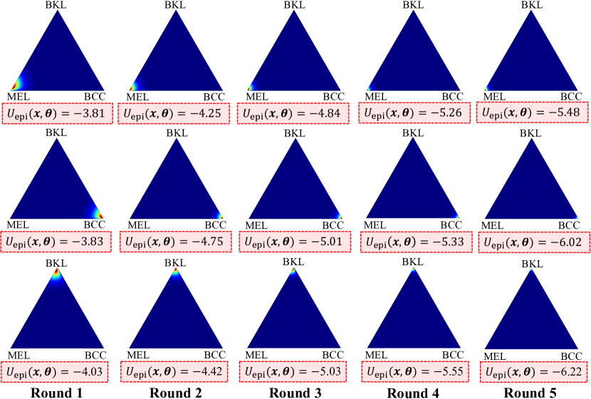
Figure 12: Visualization of the Dirichlet simplex for unlabeled samples across five FAL rounds using FEAL.

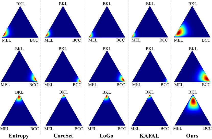
Figure 13: Visualization of the Dirichlet simplex for samples selected in the second FAL round using multiple sampling strategies.

References

- Ahn et al. [2022] Jin-Hyun Ahn, Kyungsang Kim, Jeongwan Koh, and Quanzheng Li. Federated active learning (f-al): an efficient annotation strategy for federated learning. arXiv preprint arXiv:2202.00195, 2022.
- Ash et al. [2020] Jordan T Ash, Chicheng Zhang, Akshay Krishnamurthy, John Langford, and Alekh Agarwal. Deep batch active learning by diverse, uncertain gradient lower bounds. In ICLR, 2020.
- Bandi et al. [2018] Peter Bandi, Oscar Geessink, Quirine Manson, Marcory Van Dijk, Maschenka Balkenhol, Meyke Hermsen, Babak Ehteshami Bejnordi, Byungjae Lee, Kyunghyun Paeng, Aoxiao Zhong, et al. From detection of individual metastases to classification of lymph node status at the patient level: the camelyon17 challenge. IEEE transactions on medical imaging, 38(2):550–560, 2018.
- Bernal et al. [2015] Jorge Bernal, F Javier Sánchez, Gloria Fernández-Esparrach, Debora Gil, Cristina Rodríguez, and Fernando Vilariño. Wm-dova maps for accurate polyp highlighting in colonoscopy: Validation vs. saliency maps from physicians. Computerized medical imaging and graphics, 43:99–111, 2015.
- Bloch et al. [2015] Nicholas Bloch, Anant Madabhushi, Henkjan Huisman, John Freymann, Justin Kirby, Michael Grauer, Andinet Enquobahrie, Carl Jaffe, Larry Clarke, and Keyvan Farahani. Nci-isbi 2013 challenge: automated segmentation of prostate structures. The cancer imaging archive, 370(6):5, 2015.
- Cao et al. [2023] Yu-Tong Cao, Ye Shi, Baosheng Yu, Jingya Wang, and Dacheng Tao. Knowledge-aware federated active learning with non-iid data. In ICCV, pages 22279–22289, 2023.
- Caramalau et al. [2021] Razvan Caramalau, Binod Bhattarai, and Tae-Kyun Kim. Sequential graph convolutional network for active learning. In CVPR, pages 9583–9592, 2021.
- Cassidy et al. [2022] Bill Cassidy, Connah Kendrick, Andrzej Brodzicki, Joanna Jaworek-Korjakowska, and Moi Hoon Yap. Analysis of the isic image datasets: Usage, benchmarks and recommendations. Medical image analysis, 75:102305, 2022.
- Deng et al. [2009] Jia Deng, Wei Dong, Richard Socher, Li-Jia Li, Kai Li, and Li Fei-Fei. Imagenet: A large-scale hierarchical image database. In CVPR, pages 248–255. IEEE, 2009.
- Elhamifar et al. [2013] Ehsan Elhamifar, Guillermo Sapiro, Allen Yang, and S Shankar Sasrty. A convex optimization framework for active learning. In ICCV, pages 209–216, 2013.
- Fumero et al. [2011] Francisco Fumero, Silvia Alayón, José L Sanchez, Jose Sigut, and M Gonzalez-Hernandez. Rim-one: An open retinal image database for optic nerve evaluation. In CBMS, pages 1–6. IEEE, 2011.
- Gal and Ghahramani [2016] Yarin Gal and Zoubin Ghahramani. Dropout as a bayesian approximation: representing model uncertainty in deep learning. In ICML, 2016.
- Gal et al. [2017] Yarin Gal, Riashat Islam, and Zoubin Ghahramani. Deep bayesian active learning with image data. In ICML, 2017.
- Gao et al. [2020] Mingfei Gao, Zizhao Zhang, Guo Yu, Sercan Ö Arık, Larry S Davis, and Tomas Pfister. Consistency-based semi-supervised active learning: Towards minimizing labeling cost. In ECCV, pages 510–526. Springer, 2020.
- Huang et al. [2017] Gao Huang, Zhuang Liu, Laurens Van Der Maaten, and Kilian Q Weinberger. Densely connected convolutional networks. In CVPR, pages 4700–4708, 2017.
- Huang et al. [2021] Siyu Huang, Tianyang Wang, Haoyi Xiong, Jun Huan, and Dejing Dou. Semi-supervised active learning with temporal output discrepancy. In ICCV, pages 3447–3456, 2021.
- Huang et al. [2022] Wenke Huang, Mang Ye, and Bo Du. Learn from others and be yourself in heterogeneous federated learning. In CVPR, pages 10143–10153, 2022.
- Huang et al. [2023] Wenke Huang, Mang Ye, Zekun Shi, He Li, and Bo Du. Rethinking federated learning with domain shift: A prototype view. In CVPR, pages 16312–16322. IEEE, 2023.
- Jiang et al. [2022] Meirui Jiang, Zirui Wang, and Qi Dou. Harmofl: Harmonizing local and global drifts in federated learning on heterogeneous medical images. In AAAI, pages 1087–1095, 2022.
- Jøsang [2016] Audun Jøsang. Subjective logic. Springer, 2016.
- Kim et al. [2023] SangMook Kim, Sangmin Bae, Hwanjun Song, and Se-Young Yun. Re-thinking federated active learning based on inter-class diversity. In CVPR, pages 3944–3953, 2023.
- Kingma and Ba [2014] Diederik P Kingma and Jimmy Ba. Adam: A method for stochastic optimization. arXiv preprint arXiv:1412.6980, 2014.
- Konečnỳ et al. [2016] Jakub Konečnỳ, H Brendan McMahan, Daniel Ramage, and Peter Richtárik. Federated optimization: Distributed machine learning for on-device intelligence. arXiv preprint arXiv:1610.02527, 2016.
- Kullback and Leibler [1951] Solomon Kullback and Richard A Leibler. On information and sufficiency. The annals of mathematical statistics, 22(1):79–86, 1951.
- Kutsuna et al. [2012] Natsumaro Kutsuna, Takumi Higaki, Sachihiro Matsunaga, Tomoshi Otsuki, Masayuki Yamaguchi, Hirofumi Fujii, and Seiichiro Hasezawa. Active learning framework with iterative clustering for bioimage classification. Nature communications, 3(1):1032, 2012.
- Lemaître et al. [2015] Guillaume Lemaître, Robert Martí, Jordi Freixenet, Joan C Vilanova, Paul M Walker, and Fabrice Meriaudeau. Computer-aided detection and diagnosis for prostate cancer based on mono and multi-parametric mri: a review. Computers in biology and medicine, 60:8–31, 2015.
- Li and Yin [2020] Haohan Li and Zhaozheng Yin. Attention, suggestion and annotation: a deep active learning framework for biomedical image segmentation. In MICCAI, pages 3–13. Springer, 2020.
- Li et al. [2023] Qinbin Li, Bingsheng He, and Dawn Song. Adversarial collaborative learning on non-iid features. In ICML, pages 19504–19526. PMLR, 2023.
- Li et al. [2021] Xiaoxiao Li, Meirui Jiang, Xiaofei Zhang, Michael Kamp, and Qi Dou. Fedbn: Federated learning on non-iid features via local batch normalization. arXiv preprint arXiv:2102.07623, 2021.
- Litjens et al. [2014] Geert Litjens, Robert Toth, Wendy Van De Ven, Caroline Hoeks, Sjoerd Kerkstra, Bram Van Ginneken, Graham Vincent, Gwenael Guillard, Neil Birbeck, Jindang Zhang, et al. Evaluation of prostate segmentation algorithms for mri: the promise12 challenge. Medical image analysis, 18(2):359–373, 2014.
- Liu et al. [2021] Quande Liu, Cheng Chen, Jing Qin, Qi Dou, and Pheng-Ann Heng. Feddg: Federated domain generalization on medical image segmentation via episodic learning in continuous frequency space. In CVPR, pages 1013–1023, 2021.
- Liu et al. [2020] Weitang Liu, Xiaoyun Wang, John Owens, and Yixuan Li. Energy-based out-of-distribution detection. NeurIPS, 33:21464–21475, 2020.
- MacQueen et al. [1967] James MacQueen et al. Some methods for classification and analysis of multivariate observations. In Proceedings of the fifth Berkeley symposium on mathematical statistics and probability, pages 281–297. Oakland, CA, USA, 1967.
- McMahan et al. [2017] Brendan McMahan, Eider Moore, Daniel Ramage, Seth Hampson, and Blaise Aguera y Arcas. Communication-efficient learning of deep networks from decentralized data. In Artificial intelligence and statistics, pages 1273–1282. PMLR, 2017.
- Monarch [2021] Robert Munro Monarch. Human-in-the-Loop Machine Learning: Active learning and annotation for human-centered AI. Simon and Schuster, 2021.
- Ng et al. [2011] Kai Wang Ng, Guo-Liang Tian, and Man-Lai Tang. Dirichlet and related distributions: Theory, methods and applications. 2011.
- Nguyen and Smeulders [2004] Hieu T Nguyen and Arnold Smeulders. Active learning using pre-clustering. In ICML, page 79, 2004.
- Ogier du Terrail et al. [2022] Jean Ogier du Terrail, Samy-Safwan Ayed, Edwige Cyffers, Felix Grimberg, Chaoyang He, Regis Loeb, Paul Mangold, Tanguy Marchand, Othmane Marfoq, Erum Mushtaq, et al. Flamby: Datasets and benchmarks for cross-silo federated learning in realistic healthcare settings. NeurIPS, 35:5315–5334, 2022.
- Orlando et al. [2020] José Ignacio Orlando, Huazhu Fu, João Barbosa Breda, Karel Van Keer, Deepti R Bathula, Andrés Diaz-Pinto, Ruogu Fang, Pheng-Ann Heng, Jeyoung Kim, JoonHo Lee, et al. Refuge challenge: A unified framework for evaluating automated methods for glaucoma assessment from fundus photographs. Medical image analysis, 59:101570, 2020.
- Parvaneh et al. [2022] Amin Parvaneh, Ehsan Abbasnejad, Damien Teney, Gholamreza Reza Haffari, Anton van den Hengel, and Javen Qinfeng Shi. Active learning by feature mixing. In CVPR, pages 12237–12246, 2022.
- Pearce [2020] Tim Pearce. Uncertainty in neural networks; bayesian ensembles, priors & prediction intervals. PhD thesis, University of Cambridge, 2020.
- Pearce et al. [2021] Tim Pearce, Alexandra Brintrup, and Jun Zhu. Understanding softmax confidence and uncertainty. arXiv preprint arXiv:2106.04972, 2021.
- Ronneberger et al. [2015] Olaf Ronneberger, Philipp Fischer, and Thomas Brox. U-net: Convolutional networks for biomedical image segmentation. In MICCAI, pages 234–241. Springer, 2015.
- Sener and Savarese [2017] Ozan Sener and Silvio Savarese. Active learning for convolutional neural networks: A core-set approach. arXiv preprint arXiv:1708.00489, 2017.
- Sentz and Ferson [2002] Kari Sentz and Scott Ferson. Combination of evidence in dempster-shafer theory. 2002.
- Settles [2009] Burr Settles. Active learning literature survey. 2009.
- Shannon [1948] Claude Elwood Shannon. A mathematical theory of communication. The Bell system technical journal, 27(3):379–423, 1948.
- Silva et al. [2014] Juan Silva, Aymeric Histace, Olivier Romain, Xavier Dray, and Bertrand Granado. Toward embedded detection of polyps in wce images for early diagnosis of colorectal cancer. International journal of computer assisted radiology and surgery, 9:283–293, 2014.
- Sivaswamy et al. [2015] Jayanthi Sivaswamy, S Krishnadas, Arunava Chakravarty, G Joshi, A Syed Tabish, et al. A comprehensive retinal image dataset for the assessment of glaucoma from the optic nerve head analysis. JSM biomedical imaging data papers, 2(1):1004, 2015.
- Tajbakhsh et al. [2015] Nima Tajbakhsh, Suryakanth R Gurudu, and Jianming Liang. Automated polyp detection in colonoscopy videos using shape and context information. IEEE transactions on medical imaging, 35(2):630–644, 2015.
- Tan and Le [2019] Mingxing Tan and Quoc Le. Efficientnet: Rethinking model scaling for convolutional neural networks. In ICML, pages 6105–6114. PMLR, 2019.
- Ulmer et al. [2023] Dennis Ulmer, Christian Hardmeier, and Jes Frellsen. Prior and posterior networks: A survey on evidential deep learning methods for uncertainty estimation. TMLR, 2023.
- Urner et al. [2013] Ruth Urner, Sharon Wulff, and Shai Ben-David. Plal: Cluster-based active learning. In COLT, pages 376–397. PMLR, 2013.
- Wang et al. [2023] Fan Wang, Zhongyi Han, Zhiyan Zhang, Rundong He, and Yilong Yin. Mhpl: Minimum happy points learning for active source free domain adaptation. In CVPR, pages 20008–20018, 2023.
- Wang et al. [2022a] Jiacheng Wang, Yueming Jin, and Liansheng Wang. Personalizing federated medical image segmentation via local calibration. In ECCV, pages 456–472. Springer, 2022a.
- Wang et al. [2022b] Tianyang Wang, Xingjian Li, Pengkun Yang, Guosheng Hu, Xiangrui Zeng, Siyu Huang, Cheng-Zhong Xu, and Min Xu. Boosting active learning via improving test performance. In AAAI, pages 8566–8574, 2022b.
- Wicaksana et al. [2023] Jeffry Wicaksana, Zengqiang Yan, and Kwang-Ting Cheng. Fca: Taming long-tailed federated medical image classification by classifier anchoring. arXiv preprint arXiv:2305.00738, 2023.
- Wu et al. [2022] Xing Wu, Jie Pei, Cheng Chen, Yimin Zhu, Jianjia Wang, Quan Qian, Jian Zhang, Qun Sun, and Yike Guo. Federated active learning for multicenter collaborative disease diagnosis. IEEE transactions on medical imaging, 2022.
- Yang et al. [2015] Yi Yang, Zhigang Ma, Feiping Nie, Xiaojun Chang, and Alexander G Hauptmann. Multi-class active learning by uncertainty sampling with diversity maximization. IJCV, 113:113–127, 2015.
- Yoo and Kweon [2019] Donggeun Yoo and In So Kweon. Learning loss for active learning. In CVPR, 2019.
- Yuan et al. [2023] Jiakang Yuan, Bo Zhang, Xiangchao Yan, Tao Chen, Botian Shi, Yikang Li, and Yu Qiao. Bi3d: Bi-domain active learning for cross-domain 3d object detection. In CVPR, pages 15599–15608, 2023.
- Zhang et al. [2023] Ruipeng Zhang, Qinwei Xu, Jiangchao Yao, Ya Zhang, Qi Tian, and Yanfeng Wang. Federated domain generalization with generalization adjustment. In CVPR, pages 3954–3963, 2023.