Pion axioproduction revisited

Abstract

In this work, we extend the analysis of the pion axioproduction, $aN\to\pi{N}$, to include the impact of the Roper resonance $N^{*}(1440)$ together the previously studied $\Delta(1232)$ resonance. Our theoretical framework is chiral perturbation theory with explicit resonance fields to account for their respective impacts. We find that the Roper resonance also leads to an enhancement of the cross section within its energy range for various axion models. This enhancement provided by the Roper maintains stability even when the parameter $\sin^{2}{\beta}$ of the DFSZ model undergoes variations. In contrast, the enhancement given by the $\Delta$ gradually diminishes and finally disappears as $\sin^{2}{\beta}$ approaches $1$. Furthermore, the resonance peaks given by the $\Delta$ are approximately the same in both the KSVZ model and the DFSZ model with $\sin^{2}{\beta}=\tfrac{1}{2}$, while the resonance peak given by the Roper in the former model is much more pronounced.

I Introduction

The axion is a well-motivated paradigm for physics beyond the Standard Model, simultaneously providing a solution to the strong CP problem [1, 2, 3, 4] and serving as a potential candidate for dark matter [5, 6, 7]. The original (“visible”) Peccei–Quinn–Weinberg–Wilczek (PQWW) axion with a decay constant $f_{a}$ at the electroweak scale (or equivalently a mass $m_{a}\approx 5.7\times(10^{6}\,\text{GeV}/f_{a})\,\text{eV}$ in the $\text{keV}/\text{MeV}$ region) was quickly ruled out by experiments on astrophysical grounds (axion emission from the sun and red giants) [8, 9]. Thus, the “invisible” axion was introduced with an extraordinarily large decay constant traditionally estimated to be $10^{9}\,\text{GeV}\lesssim f_{a}\lesssim 10^{12}\,\text{GeV}$ (corresponding to an axion mass between a few $\mu\text{eV}$ and $0.1\,\text{eV}$) [10], such as the Kim–Shifman–Vainstein–Zakharov (KSVZ) axion model [11, 12] or the Dine–Fischler–Srednicki–Zhitnitsky (DFSZ) axion model [13, 14].

Astrophysical observations can place stringent bounds on the properties of the axion. For instance, a core-collapse supernova (SN), e.g. SN 1987A, can emit axions in addition to neutrinos as an extra cooling mechanism of the associated neutron star. Consequently, the suppression of the neutrino luminosity due to axion emission would discernibly alter the observed neutrino events to provide stringent bounds on the axion-nucleon couplings [15, 16].

Recently, Carenza et al. [17] revisited the axion emissivity due to the pion-induced process $\pi^{-}p\to an$ and pointed out that SNe can emit axions with energies up to $500\,\text{MeV}$, which in turn can produce pions in water Cherenkov detectors via the process $aN\to\pi{N}$. At these energies, an enhanced cross section of the pion axioproduction can be expected due to the intermediate resonances. Note that we use the term axioproduction in analogy with terms like pion electro– or photoproduction. Pion axioproduction hence means pion production induced by axions. In Ref. [18], by conducting a study on the $P_{33}$ partial-wave cross section of this process, the authors confirmed the existence of such an enhancement in the $\Delta(1232)$ resonance region, which can be accessed when the axion energy $E_{a}\simeq 200\text{--}300\,\text{MeV}$. They also pointed out that the $\Delta$ contribution to the $aN\to\pi{N}$ process breaks isospin symmetry with the amplitude proportional to $(m_{d}-m_{u})/(m_{d}+m_{u})$. Thus, the enhancement of the pion axioproduction cross section estimated in Ref. [17] is reduced by 1 to 5 orders of magnitude.

In this work, we take a step further by considering also the effects of the Roper resonance $N^{*}(1440)$ on this process, whose contribution conserves isospin. This is motivated by the simple observation that the invariant mass of the initial $aN$ system falls within the $N^{*}(1440)$ resonance region when the axion energy $E_{a}$ is approximately in the range of $400\text{--}500\,\text{MeV}$, which is on the right shoulder of the bump of the SN emitted axion number spectrum from the $\pi^{-}p\to na$ process derived in Ref. [17]. Furthermore, the $N^{*}(1440)$ resonance decays into $\pi{N}$ with a large branching fraction of $(55\text{--}75)\%$ [19]. Hence, it is imperative for us to consider its impact. While the Roper does not couple as strongly as the $\Delta$ to the pion-nucleon system, the fact that the pion axioproduction via the $N^{*}$ is isopsin-conserving counteracts this suppression. In fact, we will demonstrate that the $N^{*}$ also leads to an enhancement in the cross section, and further implications for experimental detection of the axion are discussed.

We employ chiral perturbation theory (ChPT), which is a low-energy effective theory of quantum chromodynamics (QCD) [20, 21], with resonances as the theoretical framework for our study. In ChPT, the pions and nucleons, rather than the more fundamental quarks and gluons, are treated as the effective degrees of freedom, while the axion can be incorporated through external sources. Additionally, we explicitly introduce resonance fields, namely the $\Delta$ and $N^{*}$ fields, to account for their effects. This framework enables us to draw upon established knowledge of hadronic processes while at the same time preserve the spontaneously broken chiral symmetry of QCD.

The outline of this paper is as follows: In Sec. II, we collect the necessary kinematics concerning pion axioproduction. In Sec. III, we outline the main steps for incorporating the axion into ChPT. The Lagrangians describing the axion-nucleon and axion-resonance interactions are collected in Sec. IV where we also evaluate their contributions to the scattering amplitudes. Subsequently, we assemble these contributions and proceed to analyze the obtained results in Sec. V.

II Kinematics

In this section, we give a short discussion of the general isospin structure of the scattering amplitude of pion axioproduction and its partial-wave decomposition, following closely Ref. [18]. This serves to set our notation and to keep the manuscript self–contained. The process under consideration is

$$a(q)+N(p)\to\pi^{b}(q^{\prime})+N(p^{\prime}),$$ (1)

where $a$ denotes an axion, $N$ a nucleon, either proton or neutron, and $\pi^{b}$ a pion with the Cartesian isospin index $b$. As usual, we define the Lorentz-invariant Mandelstam variables:

$$s={(p+q)}^{2},\qquad t={(p-p^{\prime})}^{2},\qquad u={(p-q^{\prime})}^{2}.$$ (2)

These invariants fulfill the on-shell relation,

$$s+t+u=2m_{N}^{2}+m_{a}^{2}+M_{\pi}^{2},$$ (3)

which can be used to eliminate one of the three variables, which we choose to be $u$. In what follows, we will take the isospin-averaged nucleon mass $m_{N}=938.92\,\text{MeV}$ and the isospin-averaged pion mass $M_{\pi}=138.03\,\text{MeV}$. Throughout this paper, we use the center-of-momentum (c.m.) frame, for which the three-momenta obey the relation $\mathbf{p}+\mathbf{q}=\mathbf{p^{\prime}}+\mathbf{q^{\prime}}=0$. Using the well-known Källén function,

$$\lambda(a,b,c)=a^{2}+b^{2}+c^{2}-2ab-2ac-2bc,$$ (4)

one has

$$\begin{split}|\mathbf{p}|=|\mathbf{q}|&=\frac{\sqrt{\lambda(s,m_{N}^{2},m_{a}^{2})}}{2\sqrt{s}},\\ |\mathbf{p^{\prime}}|=|\mathbf{q^{\prime}}|&=\frac{\sqrt{\lambda(s,m_{N}^{2},M_{\pi}^{2})}}{2\sqrt{s}},\end{split}$$ (5)

and the c.m. energies of the incoming and outgoing nucleons can be written as

$$E_{\mathbf{p}}=\frac{s+m_{N}^{2}-m_{a}^{2}}{2\sqrt{s}},\qquad E_{\mathbf{p^{\prime}}}=\frac{s+m_{N}^{2}-M_{\pi}^{2}}{2\sqrt{s}}.$$ (6)

Moreover, setting $z=\cos{\theta}$, where $\theta$ is the c.m. scattering angle, we have

$$\mathbf{p}\cdot\mathbf{p^{\prime}}=|\mathbf{p}||\mathbf{p^{\prime}}|z,$$ (7)

so we can reexpress the second Mandelstam variable $t$ as

$$t=2\left(m_{N}^{2}-E_{\mathbf{p}}E_{\mathbf{p^{\prime}}}+|\mathbf{p}||\mathbf{p^{\prime}}|z\right).$$ (8)

In the following, we consider the scattering amplitude $T^{b}_{aN\to\pi{N}}$. According to the isospin structure, it can be parameterized as

$$T^{b}_{aN\to\pi{N}}=\frac{1}{2}\{\tau^{b},\tau^{3}\}T^{+}+\frac{1}{2}[\tau^{b},\tau^{3}]T^{-}+\tau^{b}T^{3},$$ (9)

which is similar to the case of $\pi{N}$ elastic scattering with isospin violation, see, e.g. Ref. [22]. Any of the four possible scattering amplitudes can then be expressed in terms of the three amplitudes $T^{+/-/3}$:

$$\begin{split}T_{ap\to\pi^{0}p}&=T^{+}+T^{3},\\ T_{an\to\pi^{0}n}&=T^{+}-T^{3},\\ T_{ap\to\pi^{+}n}&=\sqrt{2}\left(T^{-}+T^{3}\right),\\ T_{an\to\pi^{-}p}&=-\sqrt{2}\left(T^{-}-T^{3}\right).\end{split}$$ (10)

Furthermore, according to the Lorentz structure, each of the three amplitudes $T^{+/-/3}$ can be decomposed as (the superscripts are suppressed for simplicity)

$$T(s,t;\lambda^{\prime},\lambda)=\bar{u}(p^{\prime},\lambda^{\prime})\left\{A(s,t)+B(s,t)\frac{1}{2}\left(\not{q}+\not{q}^{\prime}\right)\right\}u(p,\lambda),$$ (11)

where $\lambda^{(\prime)}$, appearing in the Dirac spinor, denotes the helicity of the incoming (outgoing) nucleon. The partial-wave amplitudes $T^{l\pm}(s)$, where $l$ refers to the orbital angular momentum and the superscript $\pm$ to the total angular momentum $j=l\pm 1/2$, are given in terms of the functions $A(s,t)$ and $B(s,t)$ via

$$\begin{split}T^{l\pm}(s)=&\,\frac{\sqrt{E_{\mathbf{p}}+m_{N}}\sqrt{E_{\mathbf{p^{\prime}}}+m_{N}}}{2}\left\{A^{l}(s)+\left(\sqrt{s}-m_{N}\right)B^{l}(s)\right\}\\ &+\frac{\sqrt{E_{\mathbf{p}}-m_{N}}\sqrt{E_{\mathbf{p^{\prime}}}-m_{N}}}{2}\left\{-A^{l\pm 1}(s)+\left(\sqrt{s}+m_{N}\right)B^{l\pm 1}(s)\right\},\end{split}$$ (12)

where

$$\begin{split}A^{l}(s)&=\int_{-1}^{+1}{\text{d}z}\>{A(s,t(s,z))P_{l}(z)},\\ B^{l}(s)&=\int_{-1}^{+1}{\text{d}z}\>{B(s,t(s,z))P_{l}(z)}.\end{split}$$ (13)

The total cross section can be expanded in terms of the partial-wave cross sections as [23]

$$\sigma=\sum_{l\pm}{\sigma^{l\pm}},$$ (14)

where

$$\sigma^{l\pm}=\frac{1}{32\pi{s}}\frac{|\mathbf{p^{\prime}}|}{|\mathbf{p}|}(2l\pm 1+1){|T^{l\pm}|}^{2}.$$ (15)

In this work, we calculate the total cross section of the process $an\to\pi^{-}p$, denoted by $\sigma_{an\to\pi^{-}p}$, and the theoretical framework used to determine the corresponding partial-wave amplitudes, denoted by $T_{an\to\pi^{-}p}^{l\pm}$, is ChPT with explicit resonance fields. Particularly, we perform the calculation of the $S_{1}$, $P_{1}$ and $P_{3}$ partial-wave cross sections while neglecting the higher ones with $l\geq 2$, as those are suppressed in the energy region under consideration. Throughout, we make use of the notation $l_{2j}$, with $l=S,P,D,\cdots$ the orbital angular momentum, and $j$ the total angular momentum. Each of the partial waves contains both the isospin-conserving $(I=1/2)$ and isospin-breaking ($I=3/2$) contributions. That is, $S_{1}$ refers to the sum of both $S_{11}$ and $S_{31}$ (in the usual $l_{2I,2j}$ notation) partial waves, and so on. Since the $\Delta$ is a spin-$\tfrac{3}{2}$, positive-parity resonance and the $N^{*}(1440)$ is a spin-$\tfrac{1}{2}$, positive-parity resonance, it is reasonable to expect an enhancement in the $P_{3}$ and $P_{1}$ partial-wave cross sections in the energy region of the $\Delta$ and Roper resonances, respectively. Of course, we are well aware that the Roper does not show up as a bump in the pion-nucleon cross section and the $P_{11}$ phase shift crosses $90^{\circ}$ at an energy higher than 1.44 GeV. In case of pion axioproduction, matters can be different as the background is much suppressed.

III Incorporation of the axion into ChPT

In this section, we give a brief presentation of how the axion can be incorporated into ChPT. For a more detailed discussion, we refer to Refs. [24, 25, 26, 27]. Consider the general QCD Lagrangian with an axion below the Peccei-Quinn (PQ) symmetry breaking scale

$$\mathcal{L}_{\text{QCD}}=\mathcal{L}_{\text{QCD},0}+\frac{a}{f_{a}}{\left(\frac{g}{4\pi}\right)}^{2}\text{Tr}\left[G_{\mu\nu}\tilde{G}^{\mu\nu}\right]+\bar{q}\gamma^{\mu}\gamma_{5}\frac{\partial_{\mu}a}{2f_{a}}\mathcal{X}_{q}q,$$ (16)

where $q={(u,d,s,c,b,t)}^{\text{T}}$ collects the quark fields, $a$ refers to the axion field, and $f_{a}$ is the axion decay constant. Depending on the underlying axion model, the coupling constants of the axion-quark interactions in the matrix $\mathcal{X}_{q}=\operatorname{diag}(X_{q})$ are given by

$$\begin{split}X_{q}^{\text{KSVZ}}&=0,\\ X_{u,c,t}^{\text{DFSZ}}&=\frac{1}{3}\frac{x^{-1}}{x+x^{-1}}=\frac{1}{3}\sin^{2}{\beta},\\ X_{d,s,b}^{\text{DFSZ}}&=\frac{1}{3}\frac{x}{x+x^{-1}}=\frac{1}{3}\cos^{2}{\beta},\end{split}$$ (17)

for the KSVZ-type axion and DFSZ-type axion, respectively, where $x=\cot{\beta}$ is the ratio of the vacuum expectation values (VEVs) of the two Higgs doublets in the latter model. After a suitable axial rotation of the quark fields to remove the axion-gluon coupling term, the whole axion-quark interactions read

$$\mathcal{L}_{aq}=-(\bar{q}_{L}\mathcal{M}_{a}q_{R}+\text{h.c.})+\bar{q}\gamma^{\mu}\gamma_{5}\frac{\partial_{\mu}a}{2f_{a}}(\mathcal{X}_{q}-\mathcal{Q}_{a})q,$$ (18)

where

$$\begin{split}\mathcal{M}_{a}&=\exp{\left(i\frac{a}{f_{a}}\mathcal{Q}_{a}\right)}\mathcal{M}_{q},\\ \mathcal{Q}_{a}&=\frac{\mathcal{M}_{q}^{-1}}{\langle\mathcal{M}_{q}^{-1}\rangle}\approx\frac{1}{1+z+w}\text{diag}(1,z,w,0,0,0),\end{split}$$ (19)

with $\mathcal{M}_{q}=\text{diag}\>\{m_{q}\}$ the quark mass matrix and $z=m_{u}/m_{d}$, $w=m_{u}/m_{s}$. We take $z=0.485$ and $w=0.025$ [28].

It is from the interaction Lagrangian (18) that one has to determine the axial-vector external sources $a_{\mu}$ (isovector) and $a_{\mu}^{(s)}$ (isoscalar) that enter ChPT. In the $\text{SU}(2)$ case, this can be achieved by separating the $2$-dimensional flavor subspace of the two lightest quarks from the rest and by decomposing the matrix $\mathcal{X}_{q}-\mathcal{Q}_{a}$ into a traceless part and a part with non-vanishing trace, which results in

$$\begin{split}\mathcal{L}_{aq}=-(\bar{q}_{L}\mathcal{M}_{a}q_{R}+\text{h.c.})&+{\left(\bar{q}\gamma^{\mu}\gamma_{5}\left(c_{u-d}\frac{\partial_{\mu}a}{2f_{a}}\tau_{3}+c_{u+d}\frac{\partial_{\mu}a}{2f_{a}}\mathbbm{1}\right)q\right)}_{q={(u,d)}^{\text{T}}}\\ &+\sum_{q=\{s,c,b,t\}}\left(\bar{q}\gamma^{\mu}\gamma_{5}c_{q}\frac{\partial_{\mu}a}{2f_{a}}q\right),\end{split}$$ (20)

with

$$c_{u\pm d}=\frac{1}{2}\left(X_{u}\pm X_{d}-\frac{1\pm z}{1+z+w}\right),\quad c_{s}=X_{s}-\frac{w}{1+z+w},\quad c_{c,b,t}=X_{c,b,t}.$$ (21)

Let $c_{i}$, $i=\{1,\cdots,5\}$, refer to the isoscalar couplings $\{u+d,s,c,b,t\}$, then one finds

$$a_{\mu}=c_{u-d}\frac{\partial_{\mu}a}{2f_{a}}\tau_{3},\quad a_{\mu,i}^{(s)}=c_{i}\frac{\partial_{\mu}a}{2f_{a}}\mathbbm{1}.$$ (22)

With the usual $\text{SU}(2)$-matrix containing the three pions,

$$u=\sqrt{U}=\exp{\left(i\frac{\pi^{a}\tau_{a}}{2F}\right)},$$ (23)

where $F$ is the pion decay constant in the chiral limit, for which we take the physical value $F_{\pi}=92.4\,\text{MeV}$ as the difference only amounts to effects of higher orders than those considered here, one forms the following building blocks of ChPT:

$$\begin{split}D_{\mu}&=\partial_{\mu}+\Gamma_{\mu},\text{ with }\Gamma_{\mu}=\frac{1}{2}[u^{\dagger}\partial_{\mu}u+u\partial_{\mu}u^{\dagger}-iu^{\dagger}a_{\mu}u+iua_{\mu}u^{\dagger}],\\ u_{\mu}&=i[u^{\dagger}\partial_{\mu}u-u\partial_{\mu}u^{\dagger}-iu^{\dagger}a_{\mu}u-iua_{\mu}u^{\dagger}],\\ u_{\mu,i}&=i[-iu^{\dagger}a_{\mu,i}^{(s)}u-iua_{\mu,i}^{(s)}u^{\dagger}]=2a_{\mu,i}^{(s)}.\end{split}$$ (24)

Notice that, in principle, the axion can also enter ChPT through the building block,

$$\chi_{\pm}=u^{\dagger}\chi u^{\dagger}\pm u\chi^{\dagger}u,\text{ with }\chi=2B\mathcal{M}_{a},$$ (25)

where $B$ is a constant related to the quark condensate $\Sigma=-\langle\bar{u}u\rangle$ in the chiral limit via $B=\Sigma/F^{2}$. However, as this building block only appears in the interaction Lagrangians beyond leading order, it will not be considered in what follows.

IV Evaluation of relevant Feynman diagrams

In this section, we calculate several contributions to the scattering amplitude $T^{b}_{aN\to\pi{N}}$. First, we consider the contact and nucleon-mediated diagrams, Fig. 1, arising from the lowest order pion-nucleon Lagrangian. These diagrams start to contribute at $\mathcal{O}(q)$. At $\mathcal{O}(q^{2})$ and $\mathcal{O}(q^{3})$, there are contributions arising from the pion-nucleon Lagrangians beyond leading order. However, since axions have not been observed so far, some of the low-energy constants (LECs) of these higher-order interaction Lagrangians remain undetermined. In our approach, these contributions will be generated by the explicit exchange of the $\Delta$ and of the $N^{*}$ resonances, Figs. 2 and 3. This is a sensible assumption as explained in Ref. [29], where the dimension-two LECs were fixed from data and it was shown that resonance saturation allows to explain these values. Finally, we will then consider the $\mathcal{O}(q^{3})$ contributions from the pion rescattering loop diagram, Fig. 4. It is known that this type of contribution is most relevant for many processes at one-loop order, with the notable exception of neutral pion photoproduction off protons or neutrons [30].

IV.1 Contact term and graphs with an intermediate nucleon

In what follows, we only need the lowest order pion-nucleon Lagrangian, which is given by

$$\mathcal{L}_{\pi{N}}^{(1)}=\bar{\Psi}_{N}\left\{i\not{D}-\mathring{m}_{N}+\frac{\mathring{g}_{A}}{2}\not{u}\gamma_{5}+\frac{\mathring{g}_{0}^{i}}{2}\not{u}_{i}\gamma_{5}\right\}\Psi_{N},$$ (26)

where $\Psi_{N}={(p,n)}^{\text{T}}$ is an isodoublet containing the proton and the neutron, $\mathring{m}_{N}$ is the nucleon mass in the chiral limit, and $\mathring{g}_{A}$ and $\mathring{g}_{0}^{i}$’s are the axial-vector isovector and isoscalar coupling constants, all also in the chiral limit. In Eq. (26) and what follows, a summation over repeated $i$, the index of isoscalar couplings, is implied. Again, to the order we are working, we can identify these parameters with their physical values:

$$\mathring{g}_{A} \to g_{A} =\Delta{u}-\Delta{d},$$

$$\mathring{g}_{0}^{u-d} \to g_{0}^{u-d} =\Delta{u}+\Delta{d},$$ (27)

$$\mathring{g}_{0}^{q} \to g_{0}^{q} =\Delta{q},\text{ for }q=s,c,b,t,$$

where $s^{\mu}\Delta{q}=\langle{p}|\bar{q}\gamma^{\mu}\gamma_{5}q|p\rangle$, with $s^{\mu}$ the spin of the proton and the superscript $\mu$ denoting the polarization direction. For these matrix elements, we take the recent values from Ref. [28],

$$\Delta{u}=0.847,\quad\Delta{d}=-0.407,\quad\Delta{s}=-0.035,$$ (28)

and ignore $\Delta{q}$ for $q=c,b,t$. The relevant diagrams from $\mathcal{L}_{\pi{N}}^{(1)}$ are depicted in Fig. 1.

(a)

(b)

(c)

Figure 1: Tree-level diagrams for $aN\to\pi N$ arising from the lowest order pion-nucleon Lagrangian: (a) contact (Weinberg-Tomozawa) term, (b) $s$-channel $N$ exchange, and (c) $u$-channel $N$ exchange.

The contact (Weinberg-Tomozawa) diagram, Fig. 1a, only gives a contribution to $B^{-}$:

$$B_{\text{\ref{fig: contact}}}^{-}(s,t)=\frac{c_{u-d}}{2f_{a}F_{\pi}}.$$ (29)

For the $s$-channel nucleon-mediated diagram, Fig. 1b, we find

$$\begin{split}&A_{\text{\ref{fig: Ns}}}^{+}(s,t)=A_{\text{\ref{fig: Ns}}}^{-}(s,t)=g_{A}c_{u-d}\times A_{N}(s,t),\\ &A_{\text{\ref{fig: Ns}}}^{3}(s,t)=g_{0}^{i}c_{i}\times A_{N}(s,t),\\ &B_{\text{\ref{fig: Ns}}}^{+}(s,t)=B_{\text{\ref{fig: Ns}}}^{-}(s,t)=g_{A}c_{u-d}\times B_{N}(s,t),\\ &B_{\text{\ref{fig: Ns}}}^{3}(s,t)=g_{0}^{i}c_{i}\times B_{N}(s,t),\end{split}$$ (30)

where we have defined

$$\begin{split}A_{N}(s,t)&=\frac{g_{A}m_{N}}{2f_{a}F_{\pi}},\\ B_{N}(s,t)&=-\frac{g_{A}}{4f_{a}F_{\pi}}\left(\frac{4m_{N}^{2}}{s-m_{N}^{2}}+1\right).\end{split}$$ (31)

The $u$-channel diagram of Fig. 1c can be obtained from the former by crossing:

$$A_{\text{\ref{fig: Nu}}}^{+}(s,t) =+A_{\text{\ref{fig: Ns}}}^{+}(u,t), A_{\text{\ref{fig: Nu}}}^{-}(s,t) =-A_{\text{\ref{fig: Ns}}}^{-}(u,t), A_{\text{\ref{fig: Nu}}}^{3}(s,t) =+A_{\text{\ref{fig: Ns}}}^{3}(u,t),$$

$$B_{\text{\ref{fig: Nu}}}^{+}(s,t) =-B_{\text{\ref{fig: Ns}}}^{+}(u,t), B_{\text{\ref{fig: Nu}}}^{-}(s,t) =+B_{\text{\ref{fig: Ns}}}^{-}(u,t), B_{\text{\ref{fig: Nu}}}^{3}(s,t) =-B_{\text{\ref{fig: Ns}}}^{3}(u,t),$$ (32)

where $u$ needs to be understood as $u(s,t)$ via Eq. (3).

IV.2 Intermediate Delta and Roper resonances

Next, we consider the exchange of the $\Delta$ resonance. The interactions of the $\Delta$ with axions, pions and nucleons are given by the following effective Lagrangian, which is the leading term of an appropriate chiral invariant Lagrangian [31, 32, 33],

$$\mathcal{L}_{\Delta\pi{N}}=\frac{g}{2}\bar{\Delta}_{\mu}{T^{a\dagger}}(g^{\mu\nu}+z_{0}\gamma^{\mu}\gamma^{\nu})\langle\tau_{a}u_{\nu}\rangle\Psi_{N}+\text{h.c.},$$ (33)

where h.c. stands for the Hermitian conjugate and $\langle\>\cdots\rangle$ denotes the trace in flavor space. Here,

$$\Delta_{\mu}=\begin{pmatrix}\Delta_{\mu}^{++}\\ \Delta_{\mu}^{+}\\ \Delta_{\mu}^{0}\\ \Delta_{\mu}^{-}\end{pmatrix}$$ (34)

collects the four $\Delta$ charge eigenstates, each of which is represented by a spin-$\tfrac{3}{2}$ vector-spinor field, and $T^{a}$’s are the isospin-$\tfrac{1}{2}\!\!\to\!\!\tfrac{3}{2}$ transition matrices. The propagator of the $\Delta$ with four-momentum $p^{\mu}$ is then given by [34, 35]

$$-i\frac{\not{p}+m_{\Delta}}{p^{2}-m_{\Delta}^{2}}\left[g^{\mu\nu}-\frac{1}{3}\gamma^{\mu}\gamma^{\nu}+\frac{1}{3m_{\Delta}}\left(p^{\mu}\gamma^{\nu}-\gamma^{\mu}p^{\nu}\right)-\frac{2}{3m_{\Delta}^{2}}p^{\mu}p^{\nu}\right],$$ (35)

with $m_{\Delta}$ the mass of the $\Delta$, for which we take $m_{\Delta}=1232\,\text{MeV}$. For simplicity, we take here the Breit-Wigner rather than the pole mass, which is sufficient for the accuracy of our calculation. Moreover, the interaction Lagrangian (33) contains two coupling constants $g=-1.366$ and $z_{0}=-0.42$, whose values are taken from Ref. [36]; see Fit 2 in Table 1 therein. Notice that in the notation employed for the $\Delta$-pion-nucleon Lagrangian in Ref. [36], see Eq. (3.5) therein, two coupling constants $g_{\Delta\pi{N}}$ and $Z$ appear. They are related with the ones in Eq. (33) via $g=-\tfrac{F_{\pi}}{M_{\pi}}g_{\Delta\pi{N}}$ and $z_{0}=-(Z+\tfrac{1}{2})$. We further note that the parameter $z_{0}$ can be eliminated, but this would just change the value of $g$. Here, we prefer to work with the notation employed in Eq. (33).

(a)

(b)

Figure 2: Diagrams for $aN\to\pi{N}$ with the (a) $s$-channel and (b) $u$-channel exchange of the $\Delta$ resonance.

For the contributions from the direct exchange of the $\Delta$, Fig. 2a, we find

$$\begin{split}&A_{\text{\ref{fig: Deltas}}}^{+}(s,t)=-2A_{\text{\ref{fig: Deltas}}}^{-}(s,t)=A_{\Delta}(s,t),\\ &A_{\text{\ref{fig: Deltas}}}^{3}(s,t)=0,\\ &B_{\text{\ref{fig: Deltas}}}^{+}(s,t)=-2B_{\text{\ref{fig: Deltas}}}^{-}(s,t)=B_{\Delta}(s,t),\\ &B_{\text{\ref{fig: Deltas}}}^{3}(s,t)=0,\end{split}$$ (36)

with

$$\begin{split}A_{\Delta}(s,t)=&\,\frac{2g^{2}c_{u-d}}{3f_{a}F_{\pi}}\Biggl{\{}\frac{2z_{0}}{3m_{\Delta}^{2}}\Big{(}m_{\Delta}+\big{[}m_{N}+2m_{\Delta}\big{]}z_{0}\Big{)}\Big{(}s-m_{N}^{2}\Big{)}\\ &+\frac{1}{s-\mu_{\Delta}^{2}}\biggl{[}\Big{(}m_{N}+m_{\Delta}\Big{)}\Big{(}\frac{1}{2}\big{[}m_{a}^{2}+M_{\pi}^{2}-t\big{]}-\frac{1}{3}\big{[}s-m_{N}^{2}\big{]}\Big{)}\\ &-\frac{1}{6m_{\Delta}^{2}}\Big{(}\big{[}m_{N}+m_{\Delta}\big{]}\big{[}\big{(}m_{a}^{2}+M_{\pi}^{2}\big{)}\big{(}s-m_{N}^{2}\big{)}\\ &+m_{a}^{2}M_{\pi}^{2}\big{]}+m_{a}^{2}M_{\pi}^{2}m_{\Delta}+m_{N}{\big{[}s-m_{N}^{2}\big{]}}^{2}\Big{)}\biggr{]}\Biggr{\}},\end{split}$$ (37)

and

$$\begin{split}B_{\Delta}(s,t)=&\,\frac{2g^{2}c_{u-d}}{3f_{a}F_{\pi}}\Biggl{\{}-\frac{z_{0}}{3m_{\Delta}^{2}}\Big{(}m_{a}^{2}+M_{\pi}^{2}+2\big{[}s-m_{N}^{2}\big{]}\big{[}1+z_{0}\big{]}\\ &+4m_{N}m_{\Delta}\big{[}1+z_{0}\big{]}+4m_{N}\big{[}m_{N}+m_{\Delta}\big{]}z_{0}\Big{)}\\ &+\frac{1}{s-\mu_{\Delta}^{2}}\biggl{[}\Big{(}\frac{1}{2}\big{[}m_{a}^{2}+M_{\pi}^{2}-t\big{]}-\frac{1}{6}m_{a}^{2}+\frac{1}{6m_{\Delta}}\big{[}m_{N}+m_{\Delta}\big{]}\big{[}4m_{N}m_{\Delta}-M_{\pi}^{2}\big{]}\Big{)}\\ &-\frac{1}{6m_{\Delta}^{2}}\Big{(}\big{[}m_{a}^{2}+M_{\pi}^{2}+2m_{N}m_{\Delta}\big{]}\big{[}s-m_{N}^{2}\big{]}+m_{a}^{2}\big{[}m_{N}m_{\Delta}+M_{\pi}^{2}\big{]}+{\big{[}s-m_{N}^{2}\big{]}}^{2}\Big{)}\biggr{]}\Biggr{\}}.\end{split}$$ (38)

Notice that Eqs. (37) and (38) have a pole appearing at c.m. energies around the $\Delta$ mass. To avoid unnecessary intricacies associated with this, we use a Breit-Wigner propagator with a complex mass squared,

$$\mu_{\Delta}^{2}=m_{\Delta}^{2}-im_{\Delta}\Gamma_{\Delta},$$ (39)

with $\Gamma_{\Delta}=117\,\text{MeV}$ the width of the $\Delta$ [19]. Here, the same comment with respect to the pole value as already made for the mass applies. A more refined treatment could, e.g., be given by including the $\Delta$ self-energy in the complex mass scheme [32], but that is not required here. For the contributions from the exchange of the $\Delta$ in the crossed channel, Fig. 2b, analogous relations as the ones shown in Eq. (IV.1) hold.

Let us consider now the exchange of the $N^{*}$ resonance. The Lagrangian for the $N^{*}\pi{N}$ and $N^{*}aN$ interactions is [37, 38, 39, 40]

$$\mathcal{L}_{N^{*}\pi{N}}=\frac{\sqrt{R}}{2}\bar{\Psi}_{N^{*}}\left\{\frac{g_{A}}{2}{u\!\!\!/}\gamma_{5}+\frac{g_{0}^{i}}{2}{u\!\!\!/}_{i}\gamma_{5}\right\}\Psi_{N}+\text{h.c.},$$ (40)

with $\Psi_{N^{*}}$ the isodoublet Dirac field describing the Roper and $\sqrt{R}=0.79$ determined in Ref. [36].

(a)

(b)

Figure 3: Diagrams for $aN\to\pi N$ with the (a) $s$-channel and (b) $u$-channel exchange of the $N^{*}$ resonance.

The resulting contributions from the Roper-mediated diagrams, Figs. 3a and 3b, are similar to those from the nucleon-mediated diagrams, see Eqs. (LABEL:eq:_1b) and (IV.1), with the only difference being the need to replace $A_{N}$ and $B_{N}$ with $A_{N^{*}}$ and $B_{N^{*}}$, respectively,

$$\begin{split}A_{N^{*}}(s,t)&=\frac{Rg_{A}(m_{N}+m_{N^{*}})}{16f_{a}F_{\pi}}\frac{s-m_{N}^{2}}{s-\mu_{N^{*}}^{2}},\\ B_{N^{*}}(s,t)&=-\frac{Rg_{A}}{16f_{a}F_{\pi}}\left(\frac{2m_{N}^{2}+2m_{N}m_{N^{*}}}{s-\mu_{N^{*}}^{2}}+\frac{s-m_{N}^{2}}{s-\mu_{N^{*}}^{2}}\right),\end{split}$$ (41)

where again we used a complex mass squared in the propagator,

$$\mu_{N^{*}}^{2}=m_{N^{*}}^{2}-im_{N^{*}}\Gamma_{N^{*}},$$ (42)

with $m_{N^{*}}=1440\,\text{MeV}$ and $\Gamma_{N^{*}}=350\,\text{MeV}$ the Breit-Wigner mass and width of the Roper resonance [19]. We are well aware that such a simple parametrization does not quite represent the dynamics of the Roper in pion-nucleon scattering, see, e.g., Ref. [41] for a more refined treatment, but given the exploratory nature of our investigation, it should suffice to estimate the corresponding contribution to pion axioproduction for c.m. energies below $1.5\,\text{GeV}$.

IV.3 Pion rescattering

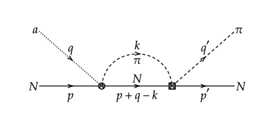
Figure 4: The pion rescattering loop diagram for $aN\to\pi N$.

The pion rescattering loop diagram is depicted in Fig. 4. The resulting contributions to the partial-wave amplitudes $T_{an\to\pi{N}}^{Il\pm}$ ($I$ denotes the isospin of the final $\pi{N}$ system) can be approximated by

$$T_{an\to\pi{N}}^{Il\pm,{\rm rescatt.}}(s)\approx T_{an\to\pi{N}}^{Il\pm,{\rm tree}}(s)\times g(s)\times T_{\pi{N}\to\pi{N}}^{Il\pm}(s).$$ (43)

The first factor, $T_{an\to\pi{N}}^{Il\pm,{\rm tree}}(s)$, corresponds to the left vertex which leads to the axion-pion conversion and, therefore, basically comprises the contributions from Fig. 1. The second factor, $g(s)$, is the usual two-point loop function involving one pion and one nucleon:

$$\begin{split}g(s)&=\frac{1}{16\pi^{2}}\left\{\tilde{a}(\mu)+\log{\left(\frac{M_{\pi}^{2}}{\mu^{2}}\right)}-x_{+}\log{\left(\frac{x_{+}-1}{x_{+}}\right)}-x_{-}\log{\left(\frac{x_{-}-1}{x_{-}}\right)}\right\},\\ x_{\pm}&=\frac{s+m_{N}^{2}-M_{\pi}^{2}}{2s}\pm\frac{1}{2s}\sqrt{{\left(s+M_{\pi}^{2}-m_{N}^{2}\right)}^{2}-4s\left(M_{\pi}^{2}-i0^{+}\right)},\end{split}$$ (44)

where we fix the regularization scale at $\mu=m_{N}$ and take the subtraction constant $\tilde{a}=-0.84$ as in Ref. [36]. Finally, the last factor, $T_{\pi{N}\to\pi{N}}^{Il\pm}(s)$, reflects the effect of the right vertex which leads to the rescattering of the pion. Since there have been many studies of pion-nucleon scattering, we do not repeat the computation of $T_{\pi{N}\to\pi{N}}^{Il\pm}(s)$ here and adopt the results of Ref. [36], see Eq. (4.11) therein.

V Results

In this section, we show and discuss the results of the total cross section of the process $an\to\pi^{-}p$, $\sigma_{an\to\pi^{-}p}$. As advocated in Sec. II, the total cross section can be approximated by the sum of the first three partial-wave cross sections,

$$\sigma\approx\sigma^{S_{1}}+\sigma^{P_{1}}+\sigma^{P_{3}}.$$ (45)

Each partial-wave cross section can be calculated by Eq. (15), and the corresponding partial-wave amplitude, $T_{an\to\pi^{-}p}^{l\pm}$, can be obtained from the calculations presented in the previous section,

$$T_{an\to\pi^{-}p}^{l\pm}=T_{an\to\pi^{-}p}^{l\pm,{\rm tree}}+T_{an\to\pi^{-}p}^{l\pm,{\rm loop}}+\mathcal{O}(q^{4}).$$ (46)

Here, $T_{an\to\pi^{-}p}^{l\pm,{\rm tree}}$ denotes the contribution arising from the tree diagrams and can be obtained by using Eqs. (10) and (12) with the functions $A$ and $B$ given in Secs. IV.1 and IV.2. $T_{an\to\pi^{-}p}^{l\pm,{\rm loop}}$ denotes the contribution originating from the loop diagram and can be expanded in terms of $T_{an\to\pi{N}}^{Il\pm,{\rm rescatt.}}$ given in Sec. IV.3 by using the isospin decomposition,

$$|\pi^{-}p\rangle=-\sqrt{\frac{2}{3}}{|I=1/2\rangle}_{\pi{N}}+\sqrt{\frac{1}{3}}{|I=3/2\rangle}_{\pi{N}}.$$ (47)

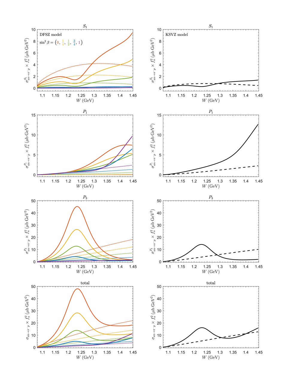
Figure 5: The total and partial-wave cross sections of $an\to\pi^{-}p$ versus the c.m. energy $W$ for the DFSZ axion at different values of $\sin^{2}{\beta}$ (left panel) and the KSVZ axion (right panel). In these plots, the solid lines correspond to the cross sections obtained based on Eq. (46), while the dashed lines correspond to the cross sections obtained considering only the contact and nucleon-mediated diagrams. In the left panel, the red, orange, green, blue and purple lines correspond to the DFSZ model parameter $\sin^{2}{\beta}=0,1/4,1/2,3/4$ and $1$, respectively.

In Fig. 5, we show the total as well as the three mentioned partial-wave cross sections as functions of the c.m. energy $W$ for the KSVZ and DFSZ models. For comparison, we also depict by dashed lines the results considering only contributions from the contact and nucleon-mediated diagrams. The cross sections are multiplied by a factor of $f_{a}^{2}$ in order to eliminate the dependence on the unknown axion decay constant. Additionally, the unknown axion decay constant also implicitly appears in the terms containing the axion mass, but it has negligible practical impact since the axion mass can safely be disregarded within the typical QCD axion window. Notice that the results of $\sin^{2}{\beta}$ taking value of $0$ in the DFSZ model is given for illustrative purposes only, as the allowed range for $\tan{\beta}$ due to the perturbative constraints from the heavy quark Yukawa couplings is $[0.25,170]$ [42] corresponding to approximately $\sin^{2}{\beta}\in[0.06,1.00]$.

As anticipated, there is indeed an enhancement in the partial-wave cross sections of $P_{3}$ and $P_{1}$ when $W\sim m_{\Delta}$ and $W\sim m_{N^{*}}$ due to the $\Delta$ and $N^{*}$, respectively. Let us first consider the $P_{3}$ partial wave. It is evident that the magnitude of the resonance peak decreases as $\sin^{2}{\beta}\to 1$ in the DFSZ model. This can be easily understood since the dominant contribution to $T_{an\to\pi^{-}p}^{P_{3}}$, arising from the $s$-channel exchange of the $\Delta$, is proportional to $c_{u-d}$ (see Eq. (LABEL:eq:_Deltas)), whose absolute value is a linearly decreasing function of $\sin^{2}{\beta}$ (see Eq. (21)): $\left|c_{u-d}^{\text{DFSZ}}(\sin^{2}{\beta})\right|=\tfrac{1}{3}\left(1.0116-\sin^{2}{\beta}\right)$. This also explains why the $P_{3}$ partial-wave result of the KSVZ model closely aligns with that of the DFSZ model when $\sin^{2}{\beta}=\tfrac{1}{2}$, as $c_{u-d}^{\text{DFSZ}}(\sin^{2}{\beta}=\tfrac{1}{2})=c_{u-d}^{\text{KSVZ}}$. We point out again that our cross section peak $f_{a}^{2}\sigma_{aN}\simeq 48-1\>\mu\text{b}\,\text{GeV}^{2}$ (for $\sin^{2}{\beta}=0-1$) is about a factor 20 to 1000 smaller than the naive estimate given in Ref. [17] because they did not account for the fact that the $\Delta$ contribution is only non-vanishing when isospin symmetry is broken. We also find that the $P_{33}$ partial-wave results of our work are smaller than those reported in Ref. [18]. This discrepancy arises from the fact that it is the isospin eigenstate considered as the initial/final states in that work. Consequently, the amplitude there takes the form of $T^{3/2}=T^{+}-T^{-}$ (see Eq. (14) therein), which can be approximated as $T^{3/2}\sim-3T^{-}$ (see Eq. (LABEL:eq:_Deltas)) if one only keeps those contributions from the $s$-channel exchange of the $\Delta$. In contrast, our analysis considers the physical initial/final states, resulting in an amplitude of $T_{an\to\pi^{-}p}=-\sqrt{2}(T^{-}-T^{3})\sim-\sqrt{2}T^{-}$. As a consequence, the peak value of cross section reported in Ref. [18] ought to be roughly $4.5$ times larger than the one we obtain, basically reflecting the differences.

In the case of $P_{1}$ partial wave, due to the relatively large decay width of the Roper, its contribution as the intermediate particle in the $s$-channel does not entirely dominate $T_{an\to\pi^{-}p}^{P_{1}}$. Therefore, the dependence of the magnitude of the resonance peak on $\sin^{2}{\beta}$ in the DFSZ model can no longer be straightforwardly understood through an analysis similar to what we did in the case of $P_{3}$ partial wave. In any case, we can still draw the following two conclusions directly from the second row in Fig. 5: First, the strength of the resonance peak remains relatively stable with variations in $\sin^{2}{\beta}$, or in other words, it does not experience significant suppression at certain values of $\sin^{2}{\beta}$. This phenomenon offers the potential for probing the DFSZ axion with $\sin^{2}{\beta}$ in the vicinity of $1$, where the resonance peak given by $\Delta$ gets highly suppressed. Taking the case where $\sin^{2}{\beta}=1$ as an example, the total cross section at $W=m_{N^{*}}$ is $10.3\>\mu\text{b}\>(\text{GeV}/f_{a})^{2}$, one order of magnitude larger than the total cross section at $W=m_{\Delta}$ taking a value of $1.2\>\mu\text{b}\>(\text{GeV}/f_{a})^{2}$. Second, the strength of the resonance peak given by the Roper in the KSVZ model is notably more pronounced than that in the DFSZ model with $\sin^{2}{\beta}=\tfrac{1}{2}$. This is in contrast to the scenario observed in the $P_{3}$ partial wave, where the strength and shape of the resonance peak given by $\Delta$ are approximately the same in both the KSVZ model and the DFSZ model with $\sin^{2}{\beta}=\tfrac{1}{2}$. If the parameter $\sin^{2}{\beta}$ of the DFSZ model happens to be around $\tfrac{1}{2}$, this feature allows us to distinguish between the two models by observing experimental results at $W\sim m_{N^{*}}$. To be more concrete, the total cross section at $W=m_{N^{*}}$ is $14.9\>\mu\text{b}\>(\text{GeV}/f_{a})^{2}$ in the KSVZ model, while only $7.4\>\mu\text{b}\>(\text{GeV}/f_{a})^{2}$ in the DFSZ model with $\sin^{2}{\beta}=\tfrac{1}{2}$.

VI Summary

In this work, we investigated the impact of the $\Delta$ and $N^{*}(1440)$ as intermediate particles on the cross section of pion axioproduction. The axions from SNe, that transform into pions in water Cherenkov detectors, can reach energies as high as $500\,\text{MeV}$, making the effects of these resonances non-negligible. The framework adopted in our study is ChPT with explicit inclusion of resonances. Based on the assumption of resonance saturation, we were able to essentially account for the effects of these resonances by explicitly considering the exchange of them in $s$-channel and $u$-channel, thereby avoiding the ignorance of LECs related to the higher-order interactions. The results indicate that an enhanced cross section is indeed present in the region of the $\Delta$ and $N^{*}(1440)$, and that experimental observations at $W\sim m_{N^{*}}$ are crucial for detecting the DFSZ axions with $\sin^{2}{\beta}$ close to $1$ as well as discerning between the KSVZ axions and the DFSZ axions with $\sin^{2}{\beta}$ around $\tfrac{1}{2}$. However, these effects are drastically reduced compared to the earlier work of Ref. [17]. Finally, considering the inverse process of pion axioproduction, $\pi{N}\to aN$, as suggested to be the dominant mechanism compared to nucleon bremsstrahlung, $NN\to aNN$, for axion production in SNe [17], it would be intriguing to explore the influence of these resonances on $\pi{N}\to aN$. Given our results, it is obvious that axioproduction is not dominating nucleon bremssrahlung but still our results show that investigating this issue may offer new insights into experimental axion searches.