DemaFormer: Damped Exponential Moving Average Transformer with Energy-Based Modeling for Temporal Language Grounding

Abstract

Temporal Language Grounding seeks to localize video moments that semantically correspond to a natural language query. Recent advances employ the attention mechanism to learn the relations between video moments and the text query. However, naive attention might not be able to appropriately capture such relations, resulting in ineffective distributions where target video moments are difficult to separate from the remaining ones. To resolve the issue, we propose an energy-based model framework to explicitly learn moment-query distributions. Moreover, we propose DemaFormer, a novel Transformer-based architecture that utilizes exponential moving average with a learnable damping factor to effectively encode moment-query inputs. Comprehensive experiments on four public temporal language grounding datasets showcase the superiority of our methods over the state-of-the-art baselines.

1 Introduction

Temporal Language Grounding (TLG) is a task to determine temporal boundaries of video moments that semantically correspond (relevant) to a language query (Hendricks et al., 2018; Gao et al., 2021a). TLG is a complex and challenging task, since video processing demands understanding across multiple modalities, including image, text, and even audio. However, TLG has received increasing attention in CV and NLP communities because it provides myriad usage for further downstream tasks, e.g. VQA (Lei et al., 2018; Ye et al., 2017; Wang et al., 2019a), relation extraction (Gao et al., 2021b), and information retrieval (Ghosh et al., 2019).

Early methods for TLG deploy concatenation with linear projection (Gao et al., 2017; Wang et al., 2019b) or similarity functions (Anne Hendricks et al., 2017; Hendricks et al., 2018) to fuse textual and visual features. To further enhance the localization performance, recent works divide the video into equal-length moments and employ the attention mechanism of the Transformer model to learn the relations between video moments and the language query. For example, Moment-DETR model (Lei et al., 2021) concatenates the visual moments and the textual tokens, and then passes the concatenated sequence to the Transformer encoder to capture the alignment. The UMT model (Liu et al., 2022) includes an additional audio channel into the Transformer encoder to construct a unified architecture.

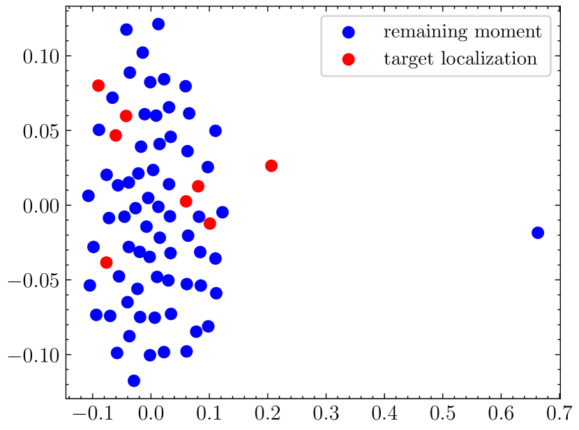
(a) UMT

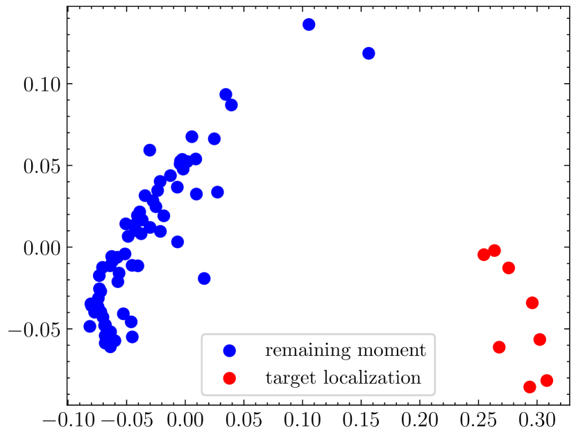
(b) DemaFormer

Figure 1: Visualization (t-SNE) of moment-query representations of an input example by the previous best UMT baseline and our DemaFormer model. The target localizations are from the QVHighlights dataset label. Detailed input content is provided in Figure 2.

Figure 2: A TLG example. To produce the output, we form the union of overlapped temporal boundaries in the groundtruth and models’ localized moments. The UMT output is about countryside scenes, which hardly align with the language query.

However, for the TLG task, previous works have shown that such attention-based approach is still insufficient to capture the rich semantic interaction between the text query and video moments (Xu et al., 2023). As in Figure 2, the localized video moments hardly align with the query statement. Moreover, the attention mechanism in the Transformer encoder does not assume any prior knowledge towards the input elements (Ma et al., 2022). For language localization, this design choice does not leverage the fact that video moments in temporal neighborhoods tend to exhibit closely related features. Therefore, this approach could lead to ineffective modeling of joint moment-query inputs. As evidence, Figure 1 demonstrates the distribution of joint moment-query representations. Particularly, the representations of target moment-query localizations and the remaining ones mingle together, making the grounding task more challenging.

To address these limitations, we dive deeper into polishing the distribution of moment-query representations. In addition to supervised training to correctly localize the language in the video, we perform unsupervised training to explicitly maximize the likelihood of moment-query localizations. This could help the multimodal model focus on capturing the distribution of target moment-query pairs and distinguishing them from others.

As such, we propose to model the distribution of moment-query representations under the framework of the Energy-Based Model (EBM). In contrast to other probabilistic models such as normalizing flow (Rezende and Mohamed, 2015) or autoencoder (Kingma and Welling, 2013), the EBM framework allows us to directly integrate the video moment’s salience score into the density function, which results in accurate modeling of moment-query representations. Our implementation develops into a contrastive divergence objective which aims to minimize the energy of the relevant localizations while maximizing the energy of the deviating ones. Accordingly, the framework needs negative samples to represent high-energy regions. Therefore, we adapt the Langevin dynamics equation to directly sample negative inputs from the EBM distribution. Such approach is appropriate because in the beginning the distribution will not match the true distribution, hence the generated samples are assured to be negative. As the training progresses, the distribution will approximate the true distribution, consequently the Langevin equation is able to produce hard negative samples.

In addition, we incorporate the inductive bias that captures local dependencies among the moment-query inputs. We propose DemaFormer in which we equip the Damped Exponential Moving Average (DEMA) computation for the TransFormer architecture. Technically, the computation applies exponentially decaying factors that consider the information from adjacent inputs. We further introduce learnable damping coefficients to enable the model to absorb adjacent information in a sufficient manner that ensures distinction among inputs. Eventually, we combine the DEMA computation with the attention mechanism to construct DemaFormer encoder and decoder modules.

To sum up, the contributions of our paper can be summarized as follows:

• We propose DemaFormer, a novel architecture for temporal language grounding. DemaFormer integrates exponential moving average with learnable damping coefficients into the attention mechanism to appropriately capture dependency patterns among video-language inputs.

• We propose a novel energy-based learning framework for temporal language grounding. The objective for the energy-based model can be formulated as a contrastive divergence to assist a classical grounding loss for modeling moment-query representations.

• We conduct extensive experiments to demonstrate the superiority of our method over previous state-of-the-art baselines. Furthermore, we conduct comprehensive ablation studies to evaluate our component proposals and deliver meaningful insights.

2 Related Work

Temporal Language Grounding (TLG). Introduced by Gao et al. (2017); Anne Hendricks et al. (2017), TLG is to locate relevant video moments given a language query. Early approaches use LSTM to encode language query and CNN for visual clips, and then estimate cross-modal similarity scores (Anne Hendricks et al., 2017; Hendricks et al., 2018). Modern techniques leverage attention mechanism and structured graph network to learn the video-language relationship (Xiao et al., 2021; Gao et al., 2021a; Zhang et al., 2020a; Yuan et al., 2019). Recent works (Liu et al., 2022; Lei et al., 2021) apply Transformer components to eliminate hand-crafted pre-processing and post-processing steps and make the model end-to-end trainable.

Vision-Language Representation Learning. Modeling the vision-language interaction is important for vision-language tasks (Gao et al., 2021a; Nguyen et al., 2022b, a, 2023; Wei et al., 2022, 2023, 2024). Previous works propose diverse techniques, including circular matrices (Wu and Han, 2018), dynamic filters (Zhang et al., 2019), Hadamard product (Zhang et al., 2020a), and contrastive learning (Nguyen and Luu, 2021). To better learn fine-grained token-level and moment-level cross-modal relations, several authors adapt graph neural networks with graph convolutional techniques (Gao et al., 2021a; Zhang et al., 2019).

3 Methodology

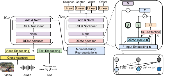
Figure 3: Illustration of the proposed DemaFormer. Our archtiecture comprises an encoder of $N_{e}$ layers and a decoder of $N_{d}$ layers. We designate the first $L_{v}$ encoder outputs as moment-query representations to become the input for the DemaFormer decoder.

Our task is to localize moments in videos from natural language queries. Formally, given a language query $q$ of $L_{q}$ tokens and a video $v$ composed of $L_{v}$ equal-length input moments, where each moment is represented by a visual frame sampled from the moment, we aim to localize $L_{m}$ time spans from $v$ that is aligned with the query $q$, noted as $\{(l_{i},r_{i})\}_{i=1}^{L_{m}}$, where each moment spans from $l_{i}$ to $r_{i}$ scaled by the video timelength and $L_{m}<L_{v}$.

Thus, we first describe our proposed damping exponential moving average attention for modeling video-language inputs in Section 3.1, the overall architecture in Section 3.2, and the training strategy empowered with energy-based modeling in Section 3.3 and 3.4.

3.1 Damping Exponential Moving Average (DEMA) Attention

In this section, we consider the input to our DemaFormer encoder $X_{e}$ and decoder $X_{d}$ in Section 3.2 as the general input $X=\{\mathbf{x}_{i}\}_{i=1}^{L_{X}}$ of length $L_{X}$. We delineate the exponential moving average (EMA) with the damping influence applied on $X$ as follows.

DEMA Computation. At first, we use a linear layer to map each input $\mathbf{x}_{i}$ to an intermediate space:

$$\mathbf{g}_{i}=\text{Linear}(\mathbf{x}_{i}),\vspace{-5pt}$$ (1)

Then, we estimate the current hidden state $\mathbf{l}_{i}$ as the sum of the previous hidden state $\mathbf{l}_{i-1}$ and the current intermediate input $\mathbf{g}_{i}$ with the weighting coefficients that decrease exponentially and are relaxed by damping coefficients:

$$\mathbf{l}_{i}=\boldsymbol{\alpha}\odot\mathbf{g}_{i}+(1-\boldsymbol{\alpha}\odot\boldsymbol{\delta})\odot\mathbf{l}_{i-1},$$ (2)

where $\boldsymbol{\alpha}\in(0,1)^{d}$ denotes the weighting coefficients, $\boldsymbol{\delta}\in(0,1)^{d}$ the damping coefficients, and $\odot$ the elementwise product. Both $\boldsymbol{\alpha}$ and $\boldsymbol{\delta}$ are randomly initialized and learnable during training. Subsequently, we project the hidden state $\mathbf{l}_{i}$ back to the original input space:

$$\mathbf{x}\textquoteright_{i}=\text{Linear}(\mathbf{l}_{i}).$$ (3)

DEMA Attention. Given the input $X$, we obtain the DEMA output in Eq. (3) and pass the output through a non-linear layer:

$$X\textquoteright=\text{DEMA}(X),$$ (4)

$$Z=\text{SiLU}(\text{Linear}(X\textquoteright)),$$ (5)

where SiLU denotes the self-gated activation function (Ramachandran et al., 2017; Elfwing et al., 2018). We experiment with other activation functions in Appendix D. Subsequently, we perform the attention operation and utilize $Z$ which exhibits local dependencies as the value tensor:

$$Q=\text{Linear}(X),$$ (6)

$$K=\text{Linear}(X),$$ (7)

$$V=\text{Linear}(Z),$$ (8)

$$Z\textquoteright=\text{softmax}\left(\frac{QK^{T}}{\sqrt{d_{K}}}\right)\cdot V,$$ (9)

where $d_{K}$ denotes the dimension of $K$. Thereafter, we aggregate the original input $X$ and the attention output $Z\textquoteright$ in an adaptive manner:

$$\boldsymbol{\lambda}=\text{sigmoid}(\text{Linear}(X\textquoteright)),$$ (10)

$$P=\text{SiLU}(\text{Linear}(X\textquoteright)+\text{Linear}(Z\odot Z\textquoteright)),$$ (11)

$$H=\boldsymbol{\lambda}\odot P+(1-\boldsymbol{\lambda})\odot X.$$ (12)

3.2 Overall Architecture

Figure 3 illustrates our DemaFormer model for temporal language grounding. We explain the architecture in details in the following.

Uni-modal Encoding. Given a video $v$ consisting of $L_{v}$ moments and a text query with $L_{q}$ tokens, we employ pre-trained models to extract visual moment features $F=\{\mathbf{f}_{i}\}_{i=1}^{L_{v}}$, textual features $T=\{\mathbf{t}_{i}\}_{i=1}^{L_{q}}$, and audio features $A=\{\mathbf{a}_{i}\}_{i=1}^{L_{v}}$.

Audio-Dependent Video Encoding. For video-audio encoding, because audio signals possess heavy noisy information (Liu et al., 2022; Badamdorj et al., 2021), we only perform 1-layer attention to fuse the audio information into the visual sequence. Particularly, the attention between the video and audio input becomes:

$$F\textquoteright=F+\text{softmax}\left(\frac{AF^{T}}{\sqrt{d}}\right)\cdot F.$$ (13)

DemaFormer Encoder. Inspired by (Lei et al., 2021), we concatenate the audio-dependent video and language tokens to form the input sequence:

$$X_{e}=[F\textquoteright,T].$$ (14)

We push the input sequence $X_{e}$ to the DemaFormer encoder of $N_{e}$ encoder layers. Each encoder layer comprises a DEMA attention layer, a normalization layer, a ReLU non-linear layer, and a residual connection:

$$H^{(i+1)}_{e}=\text{Norm}\left(\text{DEMA}\left(X_{e}^{(i)}\right)\right),$$ (15)

$$X_{e}^{(i+1)}=O_{e}^{(i)}=\text{Norm}\left(\text{ReLU}\left(H^{(i)}_{e}\right)+H^{(i)}_{e}\right).$$ (16)

where $X^{(i)}$ and $O_{e}^{(i)}$ denote the input and the output of the $i$-th encoder layer, respectively; $H_{e}^{(i)}$ the intermediate output of the $i$-th encoder layer.

We take the output of the $N_{e}$-th encoder layer as the final output $O_{e}$ of the DemaFormer encoder.

$$O_{e}=O_{e}^{(N_{e})}.$$ (17)

DemaFormer Decoder. The input for the decoder is the first $L_{v}$ DemaFormer encoder outputs, i.e. $X_{d}=\{\mathbf{o}_{e,i}\}_{i=1}^{L_{v}}$. The input sequence is forwarded to $N_{d}$ decoder layers, each of which is composed of a DEMA attention layer, a normalization layer, a non-linear layer, and a residual connection:

$$H_{d}^{(i)}=\text{Norm}\left(\text{DEMA}\left(X_{d}^{(i)}\right)\right),$$ (18)

$$M^{(i+1)}=O_{d}^{(i)}=\text{Norm}\left(\text{ReLU}\left(H^{(i)}_{d}\right)+H_{d}^{(i)}\right).$$ (19)

Analogous to the encoder, we retrieve the $N_{d}$-th layer output as the final output $O_{d}$ of the decoder:

$$O_{d}=O_{d}^{(N_{d})}.$$ (20)

Prediction Heads. For each output $\mathbf{o}_{d,i}$, we designate four separate linear layers to predict the salience score $\hat{s}_{i}$, the center $\hat{c}_{i}$, the center offset $\hat{co}_{i}$, and the moment width $\hat{w}_{i}$:

$$\hat{s}_{i}=\text{Linear}(\mathbf{o}_{d,i}),\;\hat{c}_{i}=\text{Linear}(\mathbf{o}_{d,i}),$$ (21)

$$\hat{co}_{i}=\text{Linear}(\mathbf{o}_{d,i}),\;\hat{w}_{i}=\text{Linear}(\mathbf{o}_{d,i}).$$ (22)

Thus, each candidate moment’s temporal bound becomes $\left(\hat{c}_{t}+\hat{co}_{i}-\frac{\hat{w}_{i}}{2},\hat{c}_{i}+\hat{co}_{i}+\frac{\hat{w}_{i}}{2}\right)$. At test time, we extract the top-$L_{m}$ moments whose salience scores are the largest.

3.3 Energy-Based Models for Modeling Moment-Query Representations

Given our joint video-language decoder outputs $O_{d}=\{\mathbf{o}_{d,i}\}_{t=1}^{L_{v}}$, we designate the EBM to specify the density of $O_{d}$ via the Boltzmann distribution:

$$p_{\theta}(\mathbf{o}_{d,i})=\frac{\exp(-E_{\theta}(\mathbf{o}_{d,i}))}{Z_{\theta}},$$ (23)

where $E_{\theta}$ denotes the energy function and $Z_{\theta}$ the normalizing constant $Z_{\theta}=\int\exp\left(-E_{\theta}(\mathbf{o}_{d,i})\right)\,\text{d}\mathbf{o}_{d,i}$. Inspired by (Du and Mordatch, 2019), we adopt Langevin dynamics to conduct sampling from the above distribution:

$$\tilde{\mathbf{o}}_{d,i}^{(k)}=\tilde{\mathbf{o}}_{d,i}^{(k-1)}-\frac{\gamma}{2}\nabla_{\mathbf{o}_{d,i}}E_{\theta}\left(\tilde{\mathbf{o}}_{d,i}^{(k-1)}\right)+\epsilon^{(k)},$$ (24)

$$\epsilon^{(k)}\sim\mathcal{N}(0,\gamma),\quad\tilde{\mathbf{o}}_{d,i}=\mathbf{o}^{(0)}_{d,i},$$ (25)

where $\gamma$ is a hyperparameter to specify the variance of the noise. We perform the Eq. (24) for $K$ steps and take $\tilde{\mathbf{o}}_{d,i}^{(K)}$ as the sampling outcome. Our target is to better align the video-query representation $O_{d}$, by minimizing the negative log likelihood of the moment-query representations, i.e. $\mathcal{L}_{\text{NLL}}(\theta)=-\mathbb{E}_{\mathbf{o}_{d,i}}\left[\log p_{\theta}(\mathbf{o}_{d,i})\right]$. This can be achieved by differentiating the $\mathcal{L}_{\text{NLL}}(\theta)$ and optimize the resulting contrastive divergence for the gradient, as:

$$\nabla_{\theta}\mathcal{L}_{\text{NLL}}=\mathbb{E}_{\mathbf{o}^{+}_{d,i}}\left[\nabla_{\theta}E_{\theta}(\mathbf{o}^{+}_{d,i})\right]-\mathbb{E}_{\mathbf{o}^{-}_{d,i}}\left[\nabla_{\theta}E_{\theta}(\mathbf{o}^{-}_{d,i})\right],$$ (26)

whose detailed derivation can be found in Appendix A. Because the samples generated by Eq. (24) do not approximate the true distribution in the beginning but will gradually converge to, we take these samples as $\mathbf{o}^{-}_{d,i}$ and assign their energy values a decaying weight $\alpha$ with minimum value of $\alpha_{\min}$. We take the moment-query inputs whose groundtruth salience scores are larger than a threshold $\rho$ as positive samples $\mathbf{o}^{+}_{d,i}$.

Moreover, because we maximize salience scores while minimizing the energy values of the positive input (vice versa for the negative input), we implement the negative salience-energy relation:

$$E_{\theta}(\mathbf{o}_{d,i})=-\hat{s}_{i}.$$ (27)

As such, $\theta$ becomes the DemaFormer’s parameters and we obtain the final $\mathcal{L}_{\text{NLL}}$’s formulation:

$$\alpha=\max\left(\frac{1}{1+\frac{1}{2}n_{\text{epoch}}},\alpha_{\min}\right),$$ (28)

$$\mathcal{L}_{\text{NLL}}=\mathbb{E}_{\mathbf{o}^{+}_{d,i}}\left[E_{\theta}(\mathbf{o}^{+}_{d,i})\right]-\alpha\cdot\mathbb{E}_{\mathbf{o}^{-}_{d,i}}\left[E_{\theta}(\mathbf{o}^{-}_{d,i})\right],$$ (29)

where $n_{\text{epoch}}$ denotes the current training epoch.

3.4 Training Objective

From a video-language input, we obtain $L_{m}$ predictions $\hat{Y}=\{(\hat{s}_{i},\hat{c}_{i},\hat{co}_{i},\hat{w}_{i})\}_{i=1}^{L_{m}}$. During training $L_{m}$ is the number of groundtruth localizations, while during testing $L_{m}$ is selected based on validation. We define the matching loss $L_{\text{match}}$ between predictions and groundtruth as:

$$\begin{split}\mathcal{L}_{\text{match}}=-\frac{1}{L_{m}}\sum\limits_{i=1}^{L_{m}}(\hat{s}_{i}-\lambda_{1}||c_{i}-\hat{c}_{i}||-\\ \lambda_{2}||w_{i}-\hat{w}_{i}||-\lambda_{3}||co_{i}-(\hat{co}_{i}-\hat{c}_{i})||),\end{split}$$ (30)

where $\lambda_{\{1,2,3,4\}}$ denote the hyperparameter weights for the salience, center, width, and offset losses, respectively. We jointly optimize the matching loss with the EBM negative log-likelihood (NLL) loss as follows:

$$\mathcal{L}=\mathcal{L}_{\text{match}}+\lambda_{\text{NLL}}\mathcal{L}_{\text{NLL}},$$ (31)

where $\lambda_{\text{NLL}}$ denotes the weight to scale the NLL loss size.

4 Experiments

4.1 Datasets

We evaluate our methods on four benchmark datasets for the temporal language grounding task: QVHighlights, Charades-STA, YouTube Highlights, and TVSum.

QVHighlights is collected by (Lei et al., 2021) to span diverse content on 3 major topics: daily vlog, travel vlog, and news. There are 10,148 videos with 18,367 moments associated with 10,310 queries. We follow (Lei et al., 2018; Liu et al., 2022) to split the dataset into $70\%$ train, $15\%$ val, and $15\%$ test portions.

Charades-STA (Gao et al., 2017) consists of videos about daily indoor activities. The dataset is split into 12,408 and 3,720 moment annotations for training and testing, respectively.

YouTube Highlights is prepared by (Sun et al., 2014) to comprise six categories, i.e. dog, gymnastics, parkour, skating, skiing and surfing. In each category, we inherit the original training-testing split as benchmark for the TLG task.

TVSum (Hong et al., 2020) is a video summarization dataset possessing 10 event categories. We employ the video title as the language query and the training/testing split of 0.8/0.2 for experiments.

4.2 Experimental Settings

Method	R1@		mAP@			HIT@1
	0.5	0.7	0.5	0.75	Avg.
CLIP	16.88	5.19	18.11	7.00	7.67	61.04
XML	41.83	30.35	44.63	31.73	32.14	55.25
XML+	46.69	33.46	47.89	34.67	34.90	55.06
Moment-DETR	52.89	33.02	54.82	29.40	30.73	55.60
UMT	56.23	41.18	53.83	37.01	36.12	59.99
DemaFormer (Ours)	62.39	43.94	58.25	39.36	38.71	64.77
Moment-DETR w/ PT	59.78	40.33	60.51	35.36	36.14	60.17
UMT w/ PT	60.83	43.26	57.33	39.12	38.08	62.39
DemaFormer w/ PT	63.55	45.87	59.32	41.94	40.67	65.03

Table 1: Temporal language grounding results on the QVHighlights dataset. “w/ PT” denotes pre-training with ASR captions.

Method	R1@		R5@
	0.5	0.7	0.5	0.7
MAN	41.24	20.54	83.21	51.85
2D-TAN	39.70	23.31	80.32	51.26
DRN	42.90	23.68	87.80	54.87
RaNet	43.87	26.83	86.67	54.22
Moment-DETR	48.95	21.23	86.96	50.14
UMT	49.35	26.16	89.41	54.95
DemaFormer	52.63	32.15	91.94	60.13

Table 2: Temporal language grounding results on the Charades-STA dataset.

Method	Dog	Gym.	Par.	Ska.	Ski.	Sur.	Avg.
LIM-S	57.90	41.67	66.96	57.78	48.57	65.08	56.38
DL-VHD	70.78	53.24	77.16	72.46	66.14	76.19	69.26
MINI-Net	58.24	61.68	70.20	72.18	58.68	65.06	64.43
TCG	55.41	62.69	70.86	69.11	60.08	59.79	63.02
Joint-VA	64.48	71.92	80.78	61.99	73.23	78.26	71.77
UMT	65.87	75.17	81.59	71.78	72.26	82.66	74.92
DemaFormer	71.94	77.61	86.05	78.92	74.08	83.82	77.93

Table 3: Temporal language grounding results on the YouTube Highlights dataset.

Evaluation Metrics. Our metrics include Rank k@$\mu$, mAP@$\mu$, and Hit@1. Rank k@$\mu$ is the percentage of the testing samples that have at least one correct localization in the top-$k$ choices, where a localization is correct if its IoU with the groundtruth is larger than the threshold $\mu$. In a similar manner, mAP@$\mu$ is the mean average precision of localizations whose IoU is larger than $\mu$. Hit@1 computes the hit ratio for the moment with the highest predicted salience score in a video. We consider a moment is hit if its groundtruth salience is larger than or equal to a threshold $\tau$. Following previous works (Lei et al., 2021; Liu et al., 2022), we adopt Rank 1@$\mu$ with $\mu\in\{0.5,0.75\}$ and Hit@1 with $\tau=4$ for the QVHighlights dataset. For the Charades-STA dataset, we use Rank k@$\mu$ with $k\in\{1,5\}$ and $\mu\in\{0.5,0.75\}$. We apply mAP for both the TVSum and YouTube Highlights datasets.

Implementation Details. For fair comparison with previous works (Liu et al., 2022; Lei et al., 2021), on QVHighlights, we use SlowFast (Feichtenhofer et al., 2019) and CLIP (Radford et al., 2021) to obtain features for the video moments and CLIP text encoder to obtain features for the language queries. For feature extraction of the Charades-STA dataset, we deploy VGG (Simonyan and Zisserman, 2014) and optical flow features for video moments and GloVe embeddings (Pennington et al., 2014) for language tokens. On YouTube Highlights and TVSum, we utilize the I3D model (Carreira and Zisserman, 2017) pre-trained on Kinetics 400 (Kay et al., 2017) to extract moment-level visual representations, and CLIP text encoder to extract language representations. Furthermore, as in (Liu et al., 2022; Lei et al., 2021), for QVHighlights dataset, we also experiment with pre-training our architecture with noisy automatic speech recognition (ASR) captions before fine-tuning on the downstream training samples. For all audio features, we use the PANN model pre-trained on AudioSet (Gemmeke et al., 2017). We provide detailed hyperparameter settings in Appendix B.

4.3 Baselines

To evaluate the proposed methods, we compare our performance with a diversity of baselines:

• UMT (Liu et al., 2022): a multi-modal transformer model to handle three modalities, including audio, text, and video.

• Moment-DETR (Lei et al., 2021): a multi-modal transformer model that applies the original self-attention mechanism to encode no human prior and eliminates manually-designed pre-processing and post-processing procedures.

• CLIP (Radford et al., 2021): a framework of visual CNN and textual transformer models trained with a contrastive objective.

• XML (Lei et al., 2020): a framework of visual ResNet and textual RoBERTa models with a late fusion approach to fuse the visual and textual features. We include an additional variant, XML+, which is trained with the combination of our salience loss and the XML’s loss.

• RaNet (Gao et al., 2021a): a baseline with BiLSTM text encoder, CNN image encoder, and a graph cross-modalithy interactor to learn moment-query relations and select the target moments.

• 2D-TAN (Zhang et al., 2020b): a method to specify moment candidates as a 2D map where the row and column indices indicate the starting and ending points, respectively.

• DRN (Zeng et al., 2020): a dense regression network which treats all video moments as positive and seeks to predict its distance to the groundtruth starting and ending boundaries.

• MAN (Zhang et al., 2019): a baseline with a structured graph network to model the moment-wise temporal relationships.

• TCG (Ye et al., 2021): a multi-modal TLG architecture equipped with a low-rank tensor fusion mechanism and hierarchical temporal context encoding scheme.

• Joint-VA (Badamdorj et al., 2021): an approach applying attention mechanism to fuse multi-modal features and a sentinel technique to discount noisy signals.

• MINI-Net (Hong et al., 2020): a weakly supervised learning approach that trains a positive bag of query-relevant moments to possess higher scores than negative bags of query-irrelevant moments.

• LIM-S (Xiong et al., 2019): a TLG approach that leverages video duration as a weak supervision signal.

• DL-VHD (Xu et al., 2021): a framework applying dual learners to capture cross-category concepts and video moment highlight notions.

4.4 Comparison with State-of-the-arts

Method	VT	VU	GA	MS	PK	PR	FM	BK	BT	DS	Avg.
LIM-S	55.92	42.92	61.21	53.99	60.36	47.50	43.24	66.31	69.14	62.63	56.32
DL-VHD	86.51	68.74	74.93	86.22	79.02	63.21	58.92	72.63	78.93	64.04	73.32
MINI-Net	80.64	68.31	78.16	81.83	78.11	65.82	57.84	74.99	80.22	65.49	73.14
TCG	84.96	71.43	81.92	78.61	80.18	75.52	71.61	77.34	78.57	68.13	76.83
Joint-VA	83.73	57.32	78.54	86.08	80.10	69.23	70.03	73.03	97.44	67.51	76.30
UMT	87.54	81.51	88.21	78.83	81.42	87.04	75.98	86.93	79.64	83.14	83.02
DemaFormer	88.73	85.15	92.11	88.82	82.20	89.18	80.36	89.06	98.98	85.24	87.92

Table 4: Temporal language grounding results on the TVSum dataset.

Dataset	Method	R1@
		0.5	0.7
QVHighlights	DemaFormer	62.39	43.94
	- w/o damping	60.52	42.90
	- w/o DEMA	59.42	42.06
	- w/o EBM	59.23	42.32
Charades-STA	DemaFormer	52.63	32.15
	- w/o damping	51.05	31.89
	- w/o DEMA	50.12	30.96
	- w/o EBM	49.96	30.77

Table 5: Performance comparisons on QVHighlights and Charades-STA datasets in ablative experiments of DEMA and EBM components of DemaFormer.

Energy Function	R1@		R5@
	0.5	0.7	0.5	0.7
Elementwise Cosine Similarity	51.88	31.08	90.74	59.59
Pooling-based Cosine Similarity	51.85	29.97	88.98	58.86
Salience score	52.63	32.15	91.94	60.13

Table 6: Performance comparison on the Charades-STA dataset in ablative experiments of the energy function choices.

We report results of our DemaFormer and the baselines in Table 1, 2, 3, and 4 on the QVHighlights, Charades-STA, YouTube Highlights, and TVSum datasets, respectively. As can be seen, our methods significantly outperform previous approaches.

QVHighlights. Compared with the previous best method UMT, our DemaFormer achieves $2\%$ absolute improvement at least across all evaluation settings of Rank 1@$\mu$, particularly $4.54\%$ for $\mu=0.5$ and $2.01\%$ for $\mu=0.7$, respectively. When pre-trained with the ASR captions, our method outperforms UMT with 2.59% of mAP on average and 2.64 points of Hit@1. These results demonstrate that our method can enhance the TLG operation in diverse settings, including daily vlog, travel vlog, and news.

Charades-STA. We increase the performance of UMT with $3.28\%$ in terms of Rank 1@0.5 and $2.53\%$ in terms of Rank 5@0.5. Upon tighter $\mu=0.7$, we achieve a larger degree of enhancement with $5.99\%$ for Rank 1 and $5.18\%$ for Rank 5. We hypothesize that this is because our energy-based modeling can focus on separating highly relevant localizations from other video moment candidates.

TVSum. In Table 4, we compare our model with other competitive approaches. Our architecture accomplishes the highest mAP scores across all categories and in overall as well. In detail, we outperform the second-best UMT up to $19.34\%$ at maximum on the BT portion. Analogous to the QVHighlights experiments, this demonstrates that our framework can better model the video-language inputs in various contexts to polish the temporal language grounding performance.

YouTube Highlights. Equivalent to TVSum, our DemaFormer with the energy-based modeling approach outperforms prior competitive models across various subsets. Specifically, we gain mAP increases of $1.16\%$ at minimum on the surfing portion and $6.07\%$ at maximum on the dog portion. We attribute such improvement to the more effective modeling operation of the proposed DEMA computation in attention, since it can exhibit local dependencies of moment-query inputs for appropriate modeling in various contexts.

4.5 Ablation Studies

In this section, we study the impact of (1) Damped Exponential Moving Average (DEMA), (2) Energy-Based Modeling (EBM), (3) Langevin Sampling Steps, and (4) Choice of Energy Functions.

With vs. Without DEMA. From Table 5, removing the damping factor results in slight performance decrease, for example $1.04\%$ and $0.26\%$ in terms of Rank 1@0.7 on QVHighlights and Charades-STA, respectively. The main reason is that without the damping coefficient, the model lacks the ability to adjust the information injected into adjacent input elements, such that the amount could be excessive to make it hard to distinguish video moments. Moreover, we observe that completely eliminating the DEMA computation leads to significant decrease, specifically up to $2.97\%$ and $2.51\%$ of Rank 1@0.5 respectively on QVHighlights and Charades-STA, since the model no longer specifies the moment-query distribution effectively.

With vs Without EBM. Investigating the last rows of Table 5, we realize that adopting energy-based modeling can improve the temporal language grounding performance. Particularly, adding the EBM training objective brings enhancement of $2.67\%$ on Charades-STA and $3.16\%$ on QVHighlights in terms of Rank 1@0.5. This substantiates that the EBM can successfully capture the distribution of moment-query representations in which relevant localizations are separated from the irrelevant ones. We provide more illustrative analysis in Section 4.6 and Appendix F.

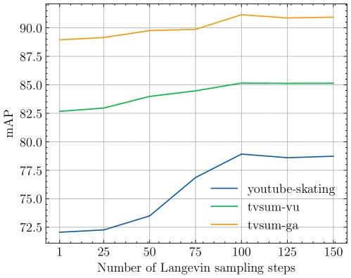
Figure 4: Effect of the number of Langevin sampling steps upon localization performance on the VU and GA portions of the TVSum dataset and the skating portion of the YouTube Highlights dataset..

Langevin Sampling Steps. We investigate the impact of the number of sampling steps $K$ in our Langevin equation (24) upon DemaFormer. Figure 4 shows that DemaFormer’s performance increases as $K$ grows. However, as long as $K$ passes the threshold $100$, the model performance converges with negligible fluctuation. We hypothesize that at $K=100$ the added noise is sufficient to segregate target localizations from elsewhere.

Choice of Energy Functions. We experiment with different choices of the energy function. Inspired by the contrastive learning works (Chuang et al., 2020; Oord et al., 2018), we compute the negative cosine similarity of video clips $O^{v}_{e}=\{\mathbf{o}_{e,i}\}_{i=1}^{L_{v}}$ and query tokens $O^{q}_{e}=\{\mathbf{o}_{e,i}\}_{i=L_{v}+1}^{L_{v}+L_{q}}$ in the elementwise and pooling-based manner (we provide the formulations in Appendix E), and evaluate the performance of the variants in Table 6. As the comparison shows, directly utilizing the salience score provides localizations with the most accuracy. This suggests that similarity functions do not fully implement the query-relevance concept.

4.6 Qualitative Analysis

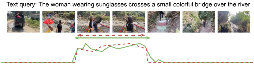
Figure 5: Qualitative visualization of DemaFormer model. Green arrow line denotes the predicted localization and green normal line the predicted salience scores. Red arrow line denotes the groundtruth localization and red normal line the annotated salience scores.

We illustrate a prediction example from the QVHighlights dataset by our DemaFormer in Figure 1, 2 and 5. We observe that our model correctly localizes target moments with respect to the user query. Our predicted salience scores also align with the groundtruth scores, which are measured by averaging the three annotated scores in the dataset. In addition, we also utilize t-SNE to visualize the moment-query representations of the example in Figure 1. We realize that the representations of the target localizations stay separately from the remaining ones, whereas those from the UMT model do mingle together. This could explain the accurate localilzation of DemaFormer and verifies the effective modeling of the proposed DEMA mechanism combined with the energy-based modeling. We provide more examples in Appendix F.

5 Conclusion

In this paper, we propose DemaFormer, a novel neural architecture for the temporal language grounding (TLG) task. By leveraging the exponential moving average approach with a damping factor, DemaFormer is capable of incorporating local dependencies among moment-query localizations. Additionally, we propose an energy-based strategy to explicitly model localization distribution. On four public benchmarks for the TLG task, our method is effective and outperforms state-of-the-art approaches with a significant margin.

6 Limitations

Our framework requires negative sampling via the Langevin dynamics equation. This incurs additional compute cost while training the language grounding model. Also, although we propose general methods to enhance the grounding performance, we have not studied their impact in cross-domain scenarios, where the model is trained upon one domain (e.g. skiing videos) and tested upon another (e.g. skating videos). We leave these gaps as future work to optimize our framework in more diverse contexts and use cases.

7 Acknowledgement

This research/project is supported by the National Research Foundation, Singapore under its AI Singapore Programme (AISG Award No: AISG3-PhD-2023-08-051T). Thong Nguyen is supported by a Google Ph.D. Fellowship in Natural Language Processing.

Appendix A Gradient of the Energy-Based Negative Log-Likelihood Objective

We have the specification of the distribution of the moment-query representations:

$$p_{\theta}(\mathbf{o})=\frac{\exp(-E_{\theta}(\mathbf{o}))}{Z_{\theta}},$$ (32)

$$Z_{\theta}=\int\exp(-E_{\theta}(\mathbf{o}))\text{d}\mathbf{o}.$$ (33)

We differentiate the negative log-likelihood of the representation:

$$-\frac{\delta\log(p_{\theta}(\mathbf{o}))}{\delta\theta}$$ (34)

$$=-\frac{\delta}{\delta\theta}\log\left(\frac{1}{Z_{\theta}}\exp(-E_{\theta}(\mathbf{o}))\right)$$ (35)

$$=-\frac{\delta}{\delta\theta}\left(-\log Z_{\theta}-E_{\theta}(\mathbf{o})\right)$$ (36)

$$=-\frac{\delta}{\delta\theta}\left(-\log\int\exp(-E_{\theta}(\mathbf{o}))\text{d}\mathbf{o}-E_{\theta}(\mathbf{o})\right)$$ (37)

$$=-\frac{1}{Z_{\theta}}\left(\int\exp(-E_{\theta})\frac{\delta E_{\theta}}{\delta\theta}\text{d}\mathbf{o}\right)+\frac{\delta E_{\theta}(\mathbf{o})}{\delta\theta}$$ (38)

$$=-\left(\frac{\delta E_{\theta}(\mathbf{o}\textquoteright)}{\delta\theta}\right)_{\mathbf{o}^{\prime}\sim p_{\theta}}+\frac{\delta E_{\theta}(\mathbf{o})}{\delta\theta}$$ (39)

$$=\nabla_{\theta}E_{\theta}(\mathbf{o}^{+})-\nabla_{\theta}E_{\theta}(\mathbf{o}^{-}).$$ (40)

We obtain the gradient formulation for the energy-based modeling component.

Appendix B Hyperparameter Settings

Our hidden dimension for the key tensor is $d_{K}=256$. Regarding our energy-based models (EBM), we adapt $K=100$ and $\gamma=0.1$ for all datasets. For the training procedure, we adopt $\lambda_{1}=\frac{1}{3},\lambda_{2}=0.01,\lambda_{3}=\frac{1}{3},\lambda_{\text{NLL}}=0.1$, and $\alpha_{\min}=0.1$. To extract positive samples to train the EBMs, we use $\rho=4,1,1$, and $0.4$ for the QVHighlights, Charades-STA, YouTube Highlights, and TVSum datasets, respectively. During testing, we adopt $L_{m}=10$ based on the validation performance. The number of DemaFormer encoder and decoder layers are set as $N_{e}=N_{d}=2$. For all training settings, we utilize the Adam optimizer with learning rate $1e-3$ and weight decay $1e-4$. We train our DemaFormer model with batch size 32 for 200 epochs on the QVHighlights, batch size 8 for 100 epochs on the Charades-STA, batch size 4 for 100 epochs on the YouTube Highlights, and batch size 1 for 500 epochs on the TVSum dataset, respectively.

Appendix C Localization Losses

Losses	R1@		mAP@			HIT@1
	0.5	0.7	0.5	0.75	Avg.
$\mathcal{L}_{s}+\mathcal{L}_{c}+\mathcal{L}_{w}$	57.29	40.97	54.29	36.61	35.98	60.84
$\mathcal{L}_{s}+\mathcal{L}_{c}+\mathcal{L}_{w}+\mathcal{L}_{oc}$	62.39	43.94	58.25	39.36	38.71	64.77

Table 7: Performance comparison on the QVHighlights dataset in ablative experiments of the influence of localization loss terms on our DemaFormer model.

Following (Liu et al., 2022; Lei et al., 2021), we conduct experiments to study the effect of localization losses on our DemaFormer architecture. We define $\mathcal{L}_{s}=-\frac{1}{L_{m}}\sum\limits_{i=1}^{L_{m}}\hat{s}_{i}$ to be the salience loss term, $\mathcal{L}_{c}=\frac{1}{L_{m}}\sum\limits_{i=1}^{L_{m}}||c_{i}-\hat{c}_{i}||$ to be the center loss term, $\mathcal{L}_{w}=\frac{1}{L_{m}}\sum\limits_{i=1}^{L_{m}}||w_{i}-\hat{w}_{i}||$ the width loss term, and $\mathcal{L}_{co}=\frac{1}{L_{m}}\sum\limits_{i=1}^{L_{m}}||co_{i}-\hat{co}_{i}||$ the center offset loss term. Because the salience, center and width terms are mandatory, we justify the necessity of the center offset term. As can be seen from Table 7, with the center offset term the localization scores increase from $54.29\%$ to $58.25\%$ of mAP@0.5, and from $40.97\%$ to $43.94\%$ of Rank 1@0.7. This demonstrates that the center offset term helps our DemaFormer architecture predict the localizations more precisely.

Appendix D Choice of Activation Functions

Activation Function	R1@		mAP@			HIT@1
	0.5	0.7	0.5	0.75	Avg.
Tanh	62.38	43.93	58.23	39.32	38.70	64.73
ReLU	62.36	43.90	58.22	39.27	38.68	64.71
GELU	62.34	43.89	58.18	39.26	38.66	64.67
SiLU	62.39	43.94	58.25	39.36	38.71	64.77

Table 8: Performance comparison on the QVHighlights dataset in ablative experiments of the activation functions.

In this appendix, we adopt different activation functions for our DEMA attention in Section 3.1 and compare their performances. In detail, we experiment with the Tanh (Dubey et al., 2022), ReLU (Dubey et al., 2022), and GELU functions (Hendrycks and Gimpel, 2016). We report the temporal language grounding performance with these activation functions on the QVHighlights dataset in Table 8. We observe that DemaFormer exhibits negligible performance fluctuation. These results demonstrate the robustness of our proposed DemaFormer with respect to the choice of activation functions.

Appendix E Specification of Energy Functions

We provide the formulation of energy functions we experiment with in Table 6.

• Element-wise cosine similarity:

  $$E_{\theta}(\mathbf{o}_{d,i})=-\frac{1}{L_{q}}\sum\limits_{j=L_{v}+1}^{L_{v}+L_{q}}\frac{\mathbf{o}_{e,i}\cdot\mathbf{o}_{e,j}}{|\mathbf{o}_{e,i}|\cdot|\mathbf{o}_{e,j}|}.$$ (41)

• Pooling-based cosine similarity:

  $$\mathbf{q}=\text{MaxPool}\{\mathbf{o}_{e,j}\}_{j=L_{v}+1}^{L_{v}+L_{q}},$$ (42)

  $$E_{\theta}(\mathbf{o}_{d,i})=-\frac{\mathbf{o}_{e,i}\cdot\mathbf{q}}{|\mathbf{o}_{e,i}|\cdot|\mathbf{q}|}.$$ (43)

• Salience score:

  $$E_{\theta}(\mathbf{o}_{d,i})=-\hat{s}_{i}.$$ (44)

Appendix F More prediction examples

In this appendix, we present more predictions of our DemaFormer model in Figure 6, 7, and 8.

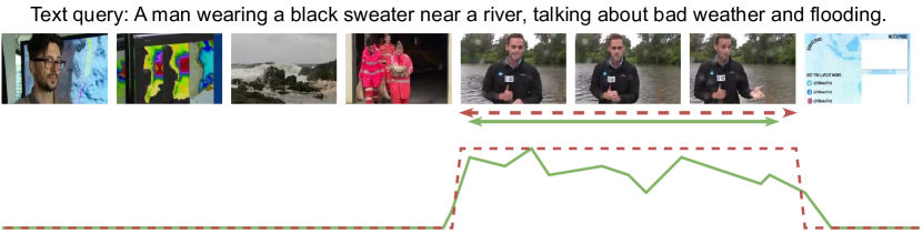
(a) Input example 1

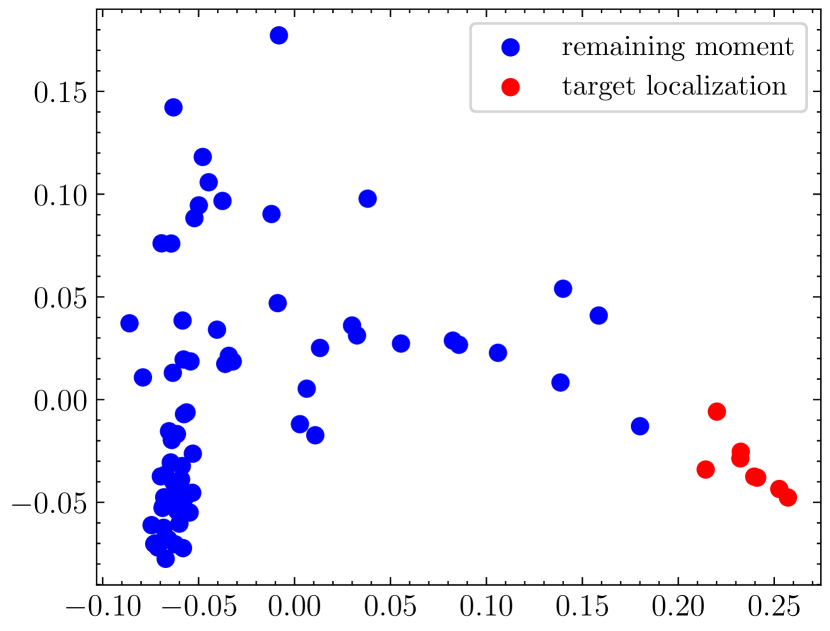
(b) DemaFormer

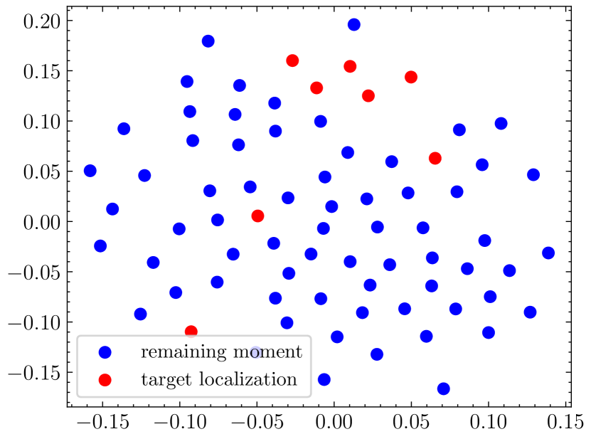
(c) UMT

Figure 6: Prediction example 1 with the t-SNE visualizations of the DemaFormer model and the UMT model. Green arrow line denotes the predicted localization and green normal line the predicted salience scores. Red arrow line denotes the groundtruth localization and red normal line the annotated salience scores.

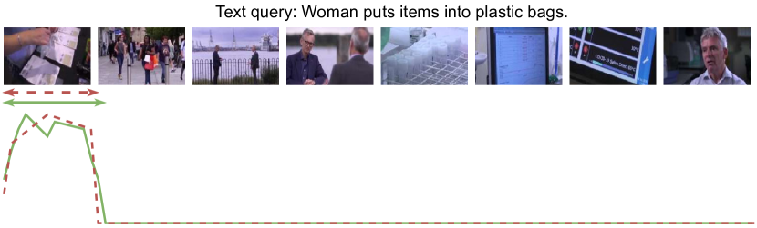
(a) Input example 2

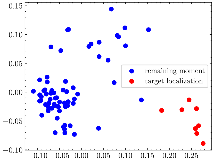
(b) DemaFormer

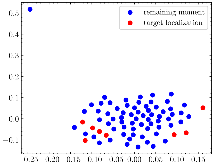
(c) UMT

Figure 7: Prediction example 2 with the t-SNE visualizations of the DemaFormer model and the UMT model. Green arrow line denotes the predicted localization and green normal line the predicted salience scores. Red arrow line denotes the groundtruth localization and red normal line the annotated salience scores.

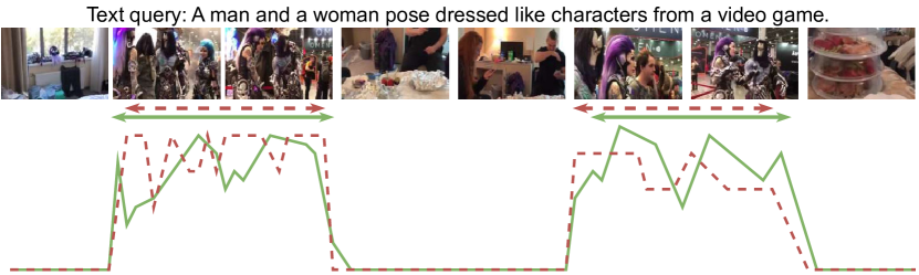
(a) Input example 3

(b) DemaFormer

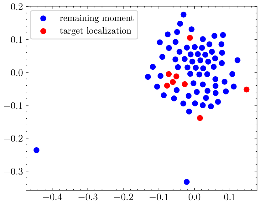
(c) UMT

Figure 8: Prediction example 3 with the t-SNE visualizations of the DemaFormer model and the UMT model. Green arrow line denotes the predicted localization and green normal line the predicted salience scores. Red arrow line denotes the groundtruth localization and red normal line the annotated salience scores.

References

- Anne Hendricks et al. (2017) Lisa Anne Hendricks, Oliver Wang, Eli Shechtman, Josef Sivic, Trevor Darrell, and Bryan Russell. 2017. Localizing moments in video with natural language. In Proceedings of the IEEE international conference on computer vision, pages 5803–5812.
- Badamdorj et al. (2021) Taivanbat Badamdorj, Mrigank Rochan, Yang Wang, and Li Cheng. 2021. Joint visual and audio learning for video highlight detection. In Proceedings of the IEEE/CVF International Conference on Computer Vision, pages 8127–8137.
- Carreira and Zisserman (2017) Joao Carreira and Andrew Zisserman. 2017. Quo vadis, action recognition? a new model and the kinetics dataset. In proceedings of the IEEE Conference on Computer Vision and Pattern Recognition, pages 6299–6308.
- Chuang et al. (2020) Ching-Yao Chuang, Joshua Robinson, Yen-Chen Lin, Antonio Torralba, and Stefanie Jegelka. 2020. Debiased contrastive learning. Advances in neural information processing systems, 33:8765–8775.
- Du and Mordatch (2019) Yilun Du and Igor Mordatch. 2019. Implicit generation and generalization in energy-based models. arXiv preprint arXiv:1903.08689.
- Dubey et al. (2022) Shiv Ram Dubey, Satish Kumar Singh, and Bidyut Baran Chaudhuri. 2022. Activation functions in deep learning: A comprehensive survey and benchmark. Neurocomputing.
- Elfwing et al. (2018) Stefan Elfwing, Eiji Uchibe, and Kenji Doya. 2018. Sigmoid-weighted linear units for neural network function approximation in reinforcement learning. Neural Networks, 107:3–11.
- Feichtenhofer et al. (2019) Christoph Feichtenhofer, Haoqi Fan, Jitendra Malik, and Kaiming He. 2019. Slowfast networks for video recognition. In Proceedings of the IEEE/CVF international conference on computer vision, pages 6202–6211.
- Gao et al. (2021a) Jialin Gao, Xin Sun, Mengmeng Xu, Xi Zhou, and Bernard Ghanem. 2021a. Relation-aware video reading comprehension for temporal language grounding. arXiv preprint arXiv:2110.05717.
- Gao et al. (2017) Jiyang Gao, Chen Sun, Zhenheng Yang, and Ram Nevatia. 2017. Tall: Temporal activity localization via language query. In Proceedings of the IEEE international conference on computer vision, pages 5267–5275.
- Gao et al. (2021b) Kaifeng Gao, Long Chen, Yifeng Huang, and Jun Xiao. 2021b. Video relation detection via tracklet based visual transformer. In Proceedings of the 29th ACM International Conference on Multimedia, pages 4833–4837.
- Gemmeke et al. (2017) Jort F Gemmeke, Daniel PW Ellis, Dylan Freedman, Aren Jansen, Wade Lawrence, R Channing Moore, Manoj Plakal, and Marvin Ritter. 2017. Audio set: An ontology and human-labeled dataset for audio events. In 2017 IEEE international conference on acoustics, speech and signal processing (ICASSP), pages 776–780. IEEE.
- Ghosh et al. (2019) Soham Ghosh, Anuva Agarwal, Zarana Parekh, and Alexander Hauptmann. 2019. Excl: Extractive clip localization using natural language descriptions. arXiv preprint arXiv:1904.02755.
- Hendricks et al. (2018) Lisa Anne Hendricks, Oliver Wang, Eli Shechtman, Josef Sivic, Trevor Darrell, and Bryan Russell. 2018. Localizing moments in video with temporal language. arXiv preprint arXiv:1809.01337.
- Hendrycks and Gimpel (2016) Dan Hendrycks and Kevin Gimpel. 2016. Gaussian error linear units (gelus). arXiv preprint arXiv:1606.08415.
- Hong et al. (2020) Fa-Ting Hong, Xuanteng Huang, Wei-Hong Li, and Wei-Shi Zheng. 2020. Mini-net: Multiple instance ranking network for video highlight detection. In Computer Vision–ECCV 2020: 16th European Conference, Glasgow, UK, August 23–28, 2020, Proceedings, Part XIII 16, pages 345–360. Springer.
- Kay et al. (2017) Will Kay, Joao Carreira, Karen Simonyan, Brian Zhang, Chloe Hillier, Sudheendra Vijayanarasimhan, Fabio Viola, Tim Green, Trevor Back, Paul Natsev, et al. 2017. The kinetics human action video dataset. arXiv preprint arXiv:1705.06950.
- Kingma and Welling (2013) Diederik P Kingma and Max Welling. 2013. Auto-encoding variational bayes. arXiv preprint arXiv:1312.6114.
- Lei et al. (2021) Jie Lei, Tamara L Berg, and Mohit Bansal. 2021. Detecting moments and highlights in videos via natural language queries. Advances in Neural Information Processing Systems, 34:11846–11858.
- Lei et al. (2018) Jie Lei, Licheng Yu, Mohit Bansal, and Tamara L Berg. 2018. Tvqa: Localized, compositional video question answering. arXiv preprint arXiv:1809.01696.
- Lei et al. (2020) Jie Lei, Licheng Yu, Tamara L Berg, and Mohit Bansal. 2020. Tvr: A large-scale dataset for video-subtitle moment retrieval. In Computer Vision–ECCV 2020: 16th European Conference, Glasgow, UK, August 23–28, 2020, Proceedings, Part XXI 16, pages 447–463. Springer.
- Liu et al. (2022) Ye Liu, Siyuan Li, Yang Wu, Chang-Wen Chen, Ying Shan, and Xiaohu Qie. 2022. Umt: Unified multi-modal transformers for joint video moment retrieval and highlight detection. In Proceedings of the IEEE/CVF Conference on Computer Vision and Pattern Recognition, pages 3042–3051.
- Ma et al. (2022) Xuezhe Ma, Chunting Zhou, Xiang Kong, Junxian He, Liangke Gui, Graham Neubig, Jonathan May, and Luke Zettlemoyer. 2022. Mega: moving average equipped gated attention. arXiv preprint arXiv:2209.10655.
- Nguyen and Luu (2021) Thong Nguyen and Anh Tuan Luu. 2021. Contrastive learning for neural topic model. Advances in neural information processing systems, 34:11974–11986.
- Nguyen et al. (2022a) Thong Nguyen, Cong-Duy Nguyen, Xiaobao Wu, See-Kiong Ng, and Anh Tuan Luu. 2022a. Vision-and-language pretraining. arXiv preprint arXiv:2207.01772.
- Nguyen et al. (2023) Thong Nguyen, Xiaobao Wu, Xinshuai Dong, Anh Tuan Luu, Cong-Duy Nguyen, Zhen Hai, and Lidong Bing. 2023. Gradient-boosted decision tree for listwise context model in multimodal review helpfulness prediction. arXiv preprint arXiv:2305.12678.
- Nguyen et al. (2022b) Thong Nguyen, Xiaobao Wu, Anh-Tuan Luu, Cong-Duy Nguyen, Zhen Hai, and Lidong Bing. 2022b. Adaptive contrastive learning on multimodal transformer for review helpfulness predictions. arXiv preprint arXiv:2211.03524.
- Oord et al. (2018) Aaron van den Oord, Yazhe Li, and Oriol Vinyals. 2018. Representation learning with contrastive predictive coding. arXiv preprint arXiv:1807.03748.
- Pennington et al. (2014) Jeffrey Pennington, Richard Socher, and Christopher D Manning. 2014. Glove: Global vectors for word representation. In Proceedings of the 2014 conference on empirical methods in natural language processing (EMNLP), pages 1532–1543.
- Radford et al. (2021) Alec Radford, Jong Wook Kim, Chris Hallacy, Aditya Ramesh, Gabriel Goh, Sandhini Agarwal, Girish Sastry, Amanda Askell, Pamela Mishkin, Jack Clark, et al. 2021. Learning transferable visual models from natural language supervision. In International conference on machine learning, pages 8748–8763. PMLR.
- Ramachandran et al. (2017) Prajit Ramachandran, Barret Zoph, and Quoc V Le. 2017. Searching for activation functions. arXiv preprint arXiv:1710.05941.
- Rezende and Mohamed (2015) Danilo Rezende and Shakir Mohamed. 2015. Variational inference with normalizing flows. In International conference on machine learning, pages 1530–1538. PMLR.
- Simonyan and Zisserman (2014) Karen Simonyan and Andrew Zisserman. 2014. Very deep convolutional networks for large-scale image recognition. arXiv preprint arXiv:1409.1556.
- Sun et al. (2014) Min Sun, Ali Farhadi, and Steve Seitz. 2014. Ranking domain-specific highlights by analyzing edited videos. In Computer Vision–ECCV 2014: 13th European Conference, Zurich, Switzerland, September 6-12, 2014, Proceedings, Part I 13, pages 787–802. Springer.
- Wang et al. (2019a) Anran Wang, Anh Tuan Luu, Chuan-Sheng Foo, Hongyuan Zhu, Yi Tay, and Vijay Chandrasekhar. 2019a. Holistic multi-modal memory network for movie question answering. IEEE Transactions on Image Processing, 29:489–499.
- Wang et al. (2019b) Weining Wang, Yan Huang, and Liang Wang. 2019b. Language-driven temporal activity localization: A semantic matching reinforcement learning model. In Proceedings of the IEEE/CVF conference on computer vision and pattern recognition, pages 334–343.
- Wei et al. (2023) Jie Wei, Guanyu Hu, Luu Anh Tuan, Xinyu Yang, and Wenjing Zhu. 2023. Multi-scale receptive field graph model for emotion recognition in conversations. In ICASSP 2023-2023 IEEE International Conference on Acoustics, Speech and Signal Processing (ICASSP), pages 1–5. IEEE.
- Wei et al. (2022) Jie Wei, Guanyu Hu, Xinyu Yang, Anh Tuan Luu, and Yizhuo Dong. 2022. Audio-visual domain adaptation feature fusion for speech emotion recognition. In INTERSPEECH, pages 1988–1992.
- Wei et al. (2024) Jie Wei, Guanyu Hu, Xinyu Yang, Anh Tuan Luu, and Yizhuo Dong. 2024. Learning facial expression and body gesture visual information for video emotion recognition. Expert Systems with Applications, 237:121419.
- Wu and Han (2018) Aming Wu and Yahong Han. 2018. Multi-modal circulant fusion for video-to-language and backward. In IJCAI, volume 3, page 8.
- Xiao et al. (2021) Shaoning Xiao, Long Chen, Jian Shao, Yueting Zhuang, and Jun Xiao. 2021. Natural language video localization with learnable moment proposals. arXiv preprint arXiv:2109.10678.
- Xiong et al. (2019) Bo Xiong, Yannis Kalantidis, Deepti Ghadiyaram, and Kristen Grauman. 2019. Less is more: Learning highlight detection from video duration. In Proceedings of the IEEE/CVF conference on computer vision and pattern recognition, pages 1258–1267.
- Xu et al. (2021) Minghao Xu, Hang Wang, Bingbing Ni, Riheng Zhu, Zhenbang Sun, and Changhu Wang. 2021. Cross-category video highlight detection via set-based learning. In Proceedings of the IEEE/CVF International Conference on Computer Vision, pages 7970–7979.
- Xu et al. (2023) Yifang Xu, Yunzhuo Sun, Yang Li, Yilei Shi, Xiaoxiang Zhu, and Sidan Du. 2023. Mh-detr: Video moment and highlight detection with cross-modal transformer. arXiv preprint arXiv:2305.00355.
- Ye et al. (2021) Qinghao Ye, Xiyue Shen, Yuan Gao, Zirui Wang, Qi Bi, Ping Li, and Guang Yang. 2021. Temporal cue guided video highlight detection with low-rank audio-visual fusion. In Proceedings of the IEEE/CVF International Conference on Computer Vision, pages 7950–7959.
- Ye et al. (2017) Yunan Ye, Zhou Zhao, Yimeng Li, Long Chen, Jun Xiao, and Yueting Zhuang. 2017. Video question answering via attribute-augmented attention network learning. In Proceedings of the 40th International ACM SIGIR conference on Research and Development in Information Retrieval, pages 829–832.
- Yuan et al. (2019) Yitian Yuan, Lin Ma, Jingwen Wang, Wei Liu, and Wenwu Zhu. 2019. Semantic conditioned dynamic modulation for temporal sentence grounding in videos. Advances in Neural Information Processing Systems, 32.
- Zeng et al. (2020) Runhao Zeng, Haoming Xu, Wenbing Huang, Peihao Chen, Mingkui Tan, and Chuang Gan. 2020. Dense regression network for video grounding. In Proceedings of the IEEE/CVF Conference on Computer Vision and Pattern Recognition, pages 10287–10296.
- Zhang et al. (2019) Da Zhang, Xiyang Dai, Xin Wang, Yuan-Fang Wang, and Larry S Davis. 2019. Man: Moment alignment network for natural language moment retrieval via iterative graph adjustment. In Proceedings of the IEEE/CVF Conference on Computer Vision and Pattern Recognition, pages 1247–1257.
- Zhang et al. (2020a) Hao Zhang, Aixin Sun, Wei Jing, and Joey Tianyi Zhou. 2020a. Span-based localizing network for natural language video localization. arXiv preprint arXiv:2004.13931.
- Zhang et al. (2020b) Songyang Zhang, Houwen Peng, Jianlong Fu, and Jiebo Luo. 2020b. Learning 2d temporal adjacent networks for moment localization with natural language. In Proceedings of the AAAI Conference on Artificial Intelligence, volume 34, pages 12870–12877.