Machine Vision Therapy: Multimodal Large Language Models Can Enhance Visual Robustness
via Denoising In-Context Learning

Abstract

Although vision models such as Contrastive Language-Image Pre-Training (CLIP) show impressive generalization performance, their zero-shot robustness is still limited under Out-of-Distribution (OOD) scenarios without fine-tuning. Instead of undesirably providing human supervision as commonly done, it is possible to take advantage of Multi-modal Large Language Models (MLLMs) that hold powerful visual understanding abilities. However, MLLMs are shown to struggle with vision problems due to the incompatibility of tasks, thus hindering their utilization. In this paper, we propose to effectively leverage MLLMs to conduct Machine Vision Therapy which aims to rectify the noisy predictions from vision models. By fine-tuning with the denoised labels, the learning model performance can be boosted in an unsupervised manner. To solve the incompatibility issue, we propose a novel Denoising In-Context Learning (DICL) strategy to align vision tasks with MLLMs. Concretely, by estimating a transition matrix that captures the probability of one class being confused with another, an instruction containing a correct exemplar and an erroneous one from the most probable noisy class can be constructed. Such an instruction can help any MLLMs with ICL ability to detect and rectify incorrect predictions of vision models. Through extensive experiments on ImageNet, WILDS, DomainBed, and other OOD datasets, we carefully validate the quantitative and qualitative effectiveness of our method. Our code is available at https://github.com/tmllab/Machine_Vision_Therapy.

1 Introduction

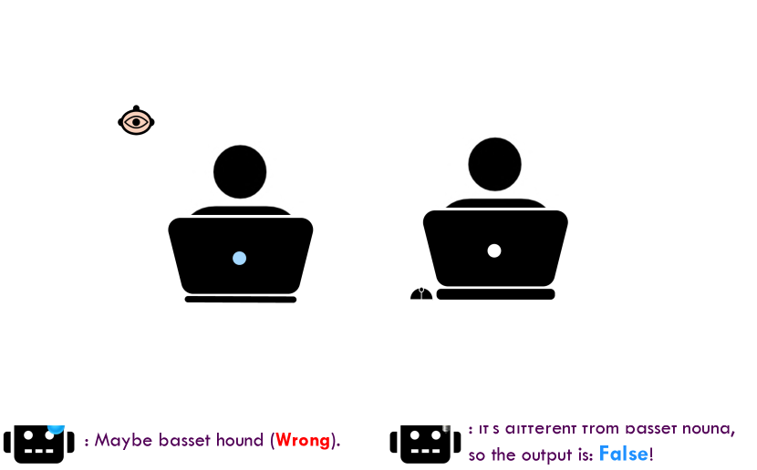
Figure 1: Illustration of our methodology: Upper row: Comparison between common fine-tuning process and fine-tuning via our Machine Vision Therapy. Our method eliminates the necessity for human-annotated data to fine-tune models by leveraging the knowledge from MLLMs. Lower row: Comparison between previous MLLM solution to vision tasks and our Denoising In-Context Learning strategy. Instead of considering all classes, our method can effectively make predictions by presenting with just a pair of positive and negative exemplars.

Pre-trained vision models such as Vision Transformers (ViT) [13, 47, 63] with Contrastive Language-Image Pre-training (CLIP) [54, 33, 42, 40, 43, 51] has been widely used thanks to their strong generalization performance and help practitioners avoid training vision models from scratch. But still, when deployed to Out-of-Distribution (OOD) circumstances [12, 21, 24, 23, 27, 31, 32, 30, 35, 61, 78], their visual recognition performance could be seriously degraded [19, 57]. Downstream fine-tuning has been a common practice to regain the generalization effectiveness [19, 64], but it requires additional label acquisition through human labor, which is undesirable for large-scale visual applications.

Fortunately, the thriving Multi-modal Large Language Models (MLLMs) [1, 2, 8, 18, 41, 39, 44, 69, 77], which take advantage of the few-shot learning ability of Large Language Models (LLM) [3, 7, 15, 53, 56, 59, 60, 76], have manifested powerful capabilities on understanding visual information with language interpretations, and excelled at recognizing novel objects in multimodal tasks such as image captioning, visual question answering, visual reasoning, etc. Considering the vulnerability of vision models under OOD situations, here we hope to refine vision models by leveraging the knowledge of MLLMs, as shown in the upper row of Figure 1. However, due to the difficulty of aligning the text generation process with visual recognition tasks such as classification [1, 62], MLLMs struggle with generating correct answers that match the ground-truth class names, thus underperform the current dominant contrastive paradigms, even when employing them as own vision encoders [1, 2, 29, 62, 72].

Focusing on enhancing the robustness of vision models, in this paper, we propose to effectively leverage MLLMs to conduct Machine Vision Therapy (MVT) which aims to diagnose and rectify the error predictions through a novel Denoising In-Context Learning (DICL) strategy. Then, we utilize the rectified supervision to guide the fine-tuning process in downstream OOD problems. Specifically, rather than giving a set of options to ask MLLMs for the exact answer [1, 29, 72], we show that it is sufficient to query for the ground truth by using only two exemplars, i.e., 1) a correct one that demonstrates the exact match between a query class name with its image example and 2) an erroneous one that combines the same query class with an image from the most confusing category for the vision model. Inspired by learning with noisy labels [22, 45, 52, 66], we can find the erroneous categories by estimating a transition matrix that captures the probability of one class being mistaken for another. By feeding the two exemplars, MLLMs can be instructed to leverage their few-shot learning power to distinguish the semantically similar images that are misclassified by vision models, as shown in the lower row of Figure 1. To process such instructions, we leverage the multi-modal in-context learning ability of several existing MLLMs [5, 38, 68, 75] to realize our methodology. After the error predictions are diagnosed and rectified, vision models can be further fine-tuned to enhance their OOD robustness on downstream data distribution. Through a comprehensive empirical study on many challenging datasets and their OOD variants, such as ImageNet [9], WILDS [35], and DomainBed [21], we carefully validate the effectiveness of our method and demonstrate its superiority over several baseline methods on many well-known vision models.

To sum up, our contributions are three-fold:

• We design a novel Machine Vision Therapy paradigm to enhance computer vision models by effectively leveraging the knowledge of MLLMs without needing additional label information.

• We propose a novel Denoising In-Context Learning strategy to successfully align MLLMs with vision tasks.

• Through comprehensive quantitative and qualitative studies on many well-known datasets, we demonstrate that the proposed method can boost the learning performance under OOD circumstances.

2 Methodology

In this section, we carefully demonstrate the Machine Vision Therapy process which mainly contains three components, namely Transition Matrix Estimation, Denoising In-Context Learning, and Fine-Tuning of vision models. Next, we first demonstrate our problem setting and give an overview of our framework. Then, we carefully elucidate the details of each part and summarize the whole process.

2.1 Problem Formulation and Overview

Generalizing to Out-of-Distribution tasks has been a challenging topic in computer vision problems, where we normally have a vision model parameterized by $\theta_{cv}\in\Theta_{cv}$ pre-trained on massive labeled in-distribution (ID) data $\mathcal{D}^{id}=\{x^{id}_{i},y^{id}_{i}\}_{i=0}^{m}$. Here each ID example $(x^{id},y^{id})\in\mathcal{X}\times\mathcal{Y}$ is sampled from a joint distribution, i.e., $(X^{id},Y^{id})\sim p^{id}$, where $X^{id}$ and $Y^{id}$ stand for variables, and $\mathcal{Y}=\mathbb{R}^{C}$. After pre-training, we can assume the conditional distribution $P(Y^{id}|X^{id})$ can be perfectly captured by the inference function $\tilde{y}^{id}=f_{\theta_{cv}}(x^{id})$, where $\tilde{y}^{id}$ is the prediction. In OOD tasks, we are given a set of unlabeled examples $\mathcal{D}^{ood}=\{x^{ood}_{i}\}_{i=0}^{n}$ whose element $x^{ood}\in\mathcal{X}$ is drawn from an unknown data distribution $p^{ood}$. Due to the change of downstream task, some factors that affect the data generating process is shifted, causing a difference between $p^{ood}$ and $p^{id}$, further hindering the label prediction, i.e., $\tilde{y}^{ood}=f_{\theta_{cv}}(x^{ood})\not\sim P(Y^{ood}|X^{ood})$, where $Y^{ood}$ is the unknown ground truth. Fortunately, having been observed with extraordinary low-shot generalization capability, we leverage MLLM with parameters $\theta_{mllm}\in\Theta_{mllm}$ to enhance the OOD robustness of vision models.

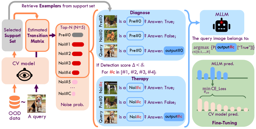
Figure 2: Workflow of our Machine Vision Therapy: The orange part demonstrates the Transition Matrix Estimation, the blue part indicates the Denoising In-Context Learning process, and the green part illustrates the Fine-Tuning of vision models.

Our framework is illustrated in Figure 2 and our problem can be formulated as follows:

$$\min_{\theta_{cv}}\mathcal{L}(f_{\theta_{cv}},h);h=\left[\theta_{mllm}((X_{i}^{+},Y_{i}^{+});(X_{i}^{-},Y_{i}^{+});X_{i})\right]_{i}^{N},\vspace{-1mm}$$ (1)

where $X_{i}^{+}$ and $X_{i}^{-}$ denotes the positive and negative exemplars, respectively, which are paired with labels $Y_{i}^{+}$ matched with $X_{i}^{+}$, $X_{i}$ is the learning example. Based on the MLLM output, we hope to fine-tune $\theta_{cv}$ by minimizing a loss function $\mathcal{L}$. Specifically, we feed all OOD data into the vision model to obtain the noisy prediction distribution $P(\tilde{Y}^{ood}|X^{ood})$, based on which we can effectively construct a support set. The support set is utilized to estimate the transition matrix and provides exemplars to instruct MLLM. Then, based on the estimated transition matrix, we use the label prediction “Pre#0” of a query image to obtain the noisy classes, in which we fix the first element to be “Pre#0” and the rest of the list contains noisy classes “Noi#c” sorted by noise probability. Further, we conduct machine vision therapy to find the possible ground truth in the top-$N$ candidates. Finally, the MLLM output is leveraged to minimize $\mathcal{L}$ to further optimize $\theta_{cv}$ during fine-tuning. Next, we explain the details of each process.

2.2 Transition Matrix Estimation

Due to the distribution shift, OOD data $x^{ood}$ could be significantly different from pre-training ID data, leading to unreliable label prediction $\tilde{y}^{ood}$. In order to capture the relationship between random variables $\tilde{Y}^{ood}$ and $Y^{ood}$, we define a transition matrix $T\in[0,1]^{C\times C}$ [45, 52, 65] which satisfies $P(Y^{ood}|X^{ood})=T^{\top}P(\tilde{Y}^{ood}|X^{ood})$. However, estimating such a transition matrix is difficult without access to any noisy label supervision or strong assumption [45, 65]. Therefore, we propose a simple yet effective sample selection approach to construct a small support set with clean labels. Specifically, to reduce the labeling workload while accurately estimating the transition matrix, we rank all OOD data within each class based on their prediction confidence, i.e., $\max_{c}\left[f_{\theta_{cv}}\right]_{c}(x^{ood})$, where $\left[f_{\theta_{cv}}\right]_{c}$ denotes the prediction probability of the $c$-th entry. From the sorted dataset $\{x_{1}^{ood,c},x_{2}^{ood,c},\cdots,x_{\frac{n}{C}}^{ood,c}\}_{c=1}^{C}$, we uniformly sample $\rho$ (labeling budget) examples from each class with interval $\frac{n}{\rho C}$, i.e., $\mathcal{D}^{supp}=\{\{x_{j\times\frac{n}{\rho C}}^{ood,c}\}_{j=1}^{\rho}\}_{c=1}^{C}$. In this way, we can cover OOD data with various noisy posterior probabilities $P(\tilde{Y}^{ood}|X^{ood})$ which further ensures the accuracy of transition matrix estimation. Then, through an acceptable labeling process, we can obtain the clean label posterior $P(Y^{ood}|X^{ood})$, thus successfully estimating the transition matrix $T$. Finally, the noise transition probability $S\in\left[0,1\right]^{C}$ of a query image can be obtained by indexing $T$ through its current noisy label prediction.

Here we further discuss several aspects of our method: 1) Why use label noise transition matrix instead of top-$N$ label predictions? Due to the particular image style and background being instance-dependent [66], the classes in top-$N$ label predictions could be completely random which does not manifest the typical feature differences and could introduce misleading signals. As a result, the ground truth may be absent from the top-$N$ label predictions under challenging scenarios. In Section 3, we carefully conduct an ablation study to validate our method; 2) Why support set is necessary for transition matrix estimation? Because there is a vital difference between our setting and common label noise learning, our problem has no access to the noisy label supervision and the latter one assumes each example contains a noisy label. Therefore, we cannot capture the noise distribution by modeling the transition matrix based on widely-used assumptions such as Anchor Point assumption [45, 65] or Cluster assumption [16].

2.3 Denoising In-Context Learning

Thanks to the previously obtained noise transition probability $S\in\left[0,1\right]^{C}$, we can further decide which one is the possible ground truth through Denoising In-Context Learning. Particularly, we only consider Top-$N$ classes with the largest noise transition probability as the potential ground truth candidates. If the label prediction denoted by “Pre#0” is not in the candidates, we would fix it in the first place. Further, we conduct a two-stage process to leverage MLLMs, namely Diagnosing and Therapy.

Diagnosing

Firstly, due to the inference time of MLLMs is actually non-trivial, if the current prediction “Pre#0” is certain, no further analysis shall be needed. Hence, to examine the fidelity of vision model predictions, our Therapy focuses on answering whether the query image belonging to class “Pre#0” is “True”. Specifically, from the aforementioned support set, we retrieve one exemplar image belonging to “Pre#0”, and another exemplar image belonging to the class with the largest noise transition probability “Noi#1”. Then, combined with the query image, we construct the in-context instruction as follows:

The symbols $<$IMG_Pre#0$>$, $<$IMG_Noi#1$>$, and $<$IMG_Query$>$ are replace tokens for the image features of exemplars from “Pre#0” and “Noi#1”, and the query image, respectively. The first example acts as the positive one to show MLLMs the true image from class “Pre#0”, and the second example shows the negative one to show the highly probable false image from “Noi#1”. Based on the current query image and its vision model prediction “Pre#0”, MLLMs can strictly follow the designed format to only output “True” or “False” token.

$$h_{0}=\theta_{mllm}(\text{pos}_{0};\text{neg}_{0};\text{query}_{i}),\vspace{-1mm}$$ (2)

where $\text{pos}_{0}$ and $\text{neg}_{0}$ denote the first positive and negative instructions, respectively, and $\text{query}_{i}$ asks whether the current prediction is correct. To enable further quantitative analysis, we obtain the logits of “True” and “False” tokens from the MLLM output and proceed with a softmax function, hence obtaining a binary probability $g_{0}=\text{softmax}(\left[h_{0}^{true},h_{0}^{false}\right])$. To decide the fidelity of “Pre#0”, we propose to not only leverage $h_{0}^{true}$ provided by MLLM but also consider the confidence from the vision model:

$$\Delta=\frac{1}{2}(h_{0}^{true}+\max_{c}\left[f_{\theta_{cv}}\right]_{c}(x^{ood})).\vspace{-1mm}$$ (3)

If the detection score $\Delta$ is larger than a threshold $\delta$, we assume the current prediction “Pre#0” is correct; otherwise, we conduct the next Therapy process.

Therapy

During therapy, we continue to utilize the instruction templates as the box above shows and traverse across the rest class candidates. Particularly, for each iteration $c$ in $N-1$ trials, we choose “Noi#c” as the positive class and “Pre#0” as the negative class, whose exemplars are correspondingly retrieved from the support set to construct the instruction. Then, it is fed into a MLLM to output whether the query image belongs to the class “Noi#c”, i.e., $h_{c}=\theta_{mllm}(\text{pos}_{c};\text{neg}_{c};\text{query}_{i}),g_{c}=\text{softmax}(\left[h_{c}^{true},h_{c}^{false}\right])$. As a result, we can decide the final prediction through:

$$y_{mllm}=\arg\max\left[h_{c}^{true}\right]_{c=0}^{C}.\vspace{-1mm}$$ (4)

After we obtain the prediction, and if it shows superior performance to the vision model, a question naturally arises: why not directly use MLLM to inference? There are three main reasons: 1) Non-negligible inference time: Because MLLMs could not handle large-batch data at a time and there are multiple traversals for one image to obtain the final prediction, it would be unimaginably slower (e.g., 1000$\times$) if only inference via MLLMs than vision models; 2) High requirements for computation: Inference through MLLM takes up huge memory of GPU. For MLLMs using large LLMs such as LLaMA-13B, it could require distributed inference for some less advanced devices; 3) Model privacy issue: Many MLLMs are highly sensitive and only provide temporary accessibility, therefore, inference through MLLM could not be always applicable. Hence, it is necessary to conduct a vision model fine-tuning based on the prediction of MLLMs.

Algorithm 1 Machine Vision Therapy.

1:Pre-trained vision model $\theta_{cv}$, MLLM $\theta_{mllm}$, unknown OOD dataset $\mathcal{D}^{ood}$.

2:Uniformly sample $\rho C$ examples from confidence-sorted $\mathcal{D}^{ood}$ to construct support set $\mathcal{D}^{supp}$;

3:Estimate transition matrix $T$; $\triangleright$ Section 2.2

4:for $i\in 0,1,\cdots,n$ do

5:    Based on the label prediction $\tilde{y}_{i}^{ood}$ to obtain the noisy transition probability $S$;

6:    Conduct Diagnosing through Eq. 2 and compute detection score $\Delta$ through Eq. 3;

7:    if $\Delta>\delta$ then

8:         Accept current prediction;

9:    else

10:         Conduct Therapy and obtain MLLM prediction through Eq. 4; $\triangleright$ Section 2.3

11:         Based on the MLLM prediction, conduct fine-tuning through Eq. 5. $\triangleright$ Section 2.4     

2.4 Fine-Tuning of Vision Models

After obtaining the MLLM prediction $y_{mllm}$, we propose to optimize vision models through the following objective:

$$min_{\theta_{cv}}CE(f_{\theta_{cv}},y_{mllm}),\vspace{-1mm}$$ (5)

where $CE(\cdot)$ denotes the cross-entropy loss that aims to minimize the loss between one distribution and a specified target. Further, we can directly deploy the fine-tuned vision models to the OOD tasks whose effectiveness is demonstrated in Section 3. Here we summarize our methodology in Algorithm 1.

3 Experiments

In this section, we first provide our experimental details. Then we conduct quantitative comparisons with the state-of-the-art vision models. Finally, we conduct ablation studies and analyses to qualitatively validate our method.

Table 1: Classification accuracy (%) of baseline CLIP models and our method on 5 ID datasets and 5 OOD datasets. We compare the performance of a VQA implementation (by directly generating answers from MLLM), our method, and the fine-tuned models supervised by our method with the baseline models, including ViT-L from CLIP [54] and ViT-g from EVA [14]. Our MVT method and the fine-tuned models have better performance.

Arch	Method	ID					OOD
		IN-Val	IN-V2	Cifar10	Cifar100	MNIST	IN-A	IN-R	IN-SK	IN-V	iWildCam
RN50	CLIP [54]	59.7	52.6	71.5	41.9	58.5	23.9	60.7	35.4	31.1	8.2
RN101		61.7	56.2	80.8	48.8	51.6	30.2	66.7	40.9	35.4	12.3
ViT-B		62.9	56.1	89.9	65.0	47.9	32.2	67.9	41.9	30.5	10.9
ViT-L	CLIP [54]	75.8	70.2	95.6	78.2	76.4	69.3	86.6	59.4	51.8	13.4
	VQA	64.9	59.9	97.6	83.2	56.7	66.0	87.3	56.9	56.2	13.3
	MVT	75.2	70.8	97.9	78.9	53.0	71.2	88.1	59.0	62.1	25.0
	+FT	76.9	70.5	96.7	82.0	79.2	75.1	89.5	61.4	68.8	-
ViT-g	EVA [14]	78.8	71.2	98.3	88.8	62.2	71.9	91.4	67.7	64.9	21.9
	VQA	64.3	59.6	97.9	84.5	55.7	64.6	87.4	58.2	59.2	19.7
	MVT	79.1	71.6	98.1	89.0	63.2	73.2	91.4	67.9	66.3	25.1
	+FT	79.0	72.2	98.9	91.2	65.7	75.5	92.8	68.6	70.6	-

3.1 Experiments Setup

3.1.1 Datasets and Models

Datasets. In our experiments, we leverages well-known ID datasets including ImageNet-1K [9] validation dataset, ImageNet-V2 [55], Cifar10 [36], Cifar100 [36] and MNIST [37]. We also evaluate OOD generalization on datasets that are commonly considered OOD ones:

• ImageNet-A [27]: The ImageNet-A dataset consists of 7,500 real-world, unmodified, and naturally occurring examples, drawn from some challenging scenarios.

• ImageNet-R [26]: The ImageNet-R dataset contains 16 different renditions (eg. art, cartoons, deviantart, etc).

• ImageNet-Sketch [61]: The ImageNet-Sketch dataset consists of 50000 black and white sketch images, 50 images for each of the 1000 ImageNet classes.

• ImageNet-V [11]: The ImageNet-V is an OOD dataset for benchmarking viewpoint robustness of visual classifiers, which is generated by viewfool, and has 10,000 renderings of 100 objects with images of size 400$\times$400.

• iWildCam [34] is from a benchmark dataset of in-the-wild distribution shifts. It contains wild animal pictures captured under various environmental conditions.

• DomainBed [20]: DomainBed is a dataset of common objects in 6 different domains, each of which includes 345 categories of objects.

Models. For backbone models, we primarily employ CLIP models from the original version [54] and utilize ViT-L/14 as the vision model to be enhanced. Additionally, we also employ ViT-g [71] from EVA [14] as an alternative vision model. For MLLM backbone, we consider two existing works MMICL [75] and Otter [39] that possess miltimodal ICL ability. Specifically, MMICL adopts BLIP-2 [41] as the vision encoder and FLAN-T5-XXL [7] as the language model. On the other hand, Otter leverages OpenFlamingo [2] as the backbone model. To provide a comparative analysis, we also assess the performance of CLIP variants that employ ResNet50, ResNet101, and ViT-B/32 as alternative vision encoders.

Table 2: Classification accuracy (%) of baseline CLIP models and our method on 4 subsets of DomainBed datasets, including VLCS, PACS, OfficeHome, and DomainNet. We compare the performance of our method and the fine-tuned models supervised by our method with the baseline models, including ViT-L from CLIP [54] and ViT-g from EVA [14]. The fine-tuned models with our MVT method have the best performance.

	Datasets	VLCS				PACS				OfficeHome				DomainNet					Avg
	method	0	1	2	3	0	1	2	3	0	1	2	3	0	1	2	3	4
ViT-L	CLIP [54]	74.9	83.5	80.3	74.5	97.8	97.4	97.5	99.4	87.7	92.7	85.7	85.6	61.1	62.1	60.2	78.4	51.1	80.6
	MVT	83.8	89.0	87.2	80.3	97.6	97.5	98.0	99.4	87.7	93.4	89.0	88.5	61.3	62.1	60.4	78.7	53.4	82.8
	+FT	84.2	89.8	87.9	82.5	98.0	98.2	98.0	99.8	90.9	95.0	90.9	90.8	62.5	63.8	62.4	80.1	54.0	84.0
ViT-g	EVA [14]	72.5	80.0	79.8	72.8	99.0	98.8	98.9	99.8	90.5	94.2	88.6	88.7	61.4	64.7	61.2	81.6	54.9	81.6
	MVT	81.2	86.6	86.1	79.5	98.2	98.0	98.0	99.4	89.7	93.8	89.7	89.1	62.2	65.0	61.6	82.3	56.1	83.3
	+FT	83.7	89.5	86.9	82.0	99.1	98.9	99.0	100.0	91.6	95.1	90.7	90.6	61.9	64.8	63.2	81.9	56.6	84.4

3.1.2 Evaluation Settings

For model evaluation, we randomly select 5000 images independently from the ImageNet validation set (IN-Val), ImageNet-V2 (IN-V2), ImageNet-A (IN-A), ImageNet-R (IN-R), ImageNet-Sketch (IN-SK), ImageNet-V (IN-V) and 10000 images independently from Cifar10, Cifar100, MNIST to constitute the test samples. Additionally, we select $3$ images per category to construct a support set to provide in-context exemplars. In the main paper, we evaluate iWildCam from WILDS and VLCS, PACS, OfficeHome, and DomainNet from DomainBed.

For the details of implementation, we first estimate the transition matrix through the proposed sample selection approach which is based on the support set, then we find the top-$6$ noisy classes which are further used to conduct MVT. Concretely, we set the threshold $\delta=0.6$ to diagnose incorrect predictions, then we retrieve exemplars from the support set based on the most similar logit prediction as the learning image and conduct DICL. The retrieved exemplars contain only one positive and negative pair. For each round of DICL, we repeat the process for $3$ times and average the model predictions. To this end, we can obtain our MLLM prediction which is further leveraged to conduct vision model fine-tuning. Particularly, we optimize the CLIP vision encoder for $3$ epochs using Adam and SGD optimizers for ViT-L and ViT-g, respectively. Other details and datasets are shown in Appendix.

3.2 Quantitative Comparison

First, we compare our MVT method with well-known vision models under both ID and OOD scenarios. As shown in Table 1, we can see that the method with “+FT” which denotes fine-tuning achieves better performance on most settings. Specifically, on “IN-V”, our method with fine-tuning can significantly surpass both CLIP and EVA for $17\%$ and $6\%$, respectively. Moreover, on “IN-A”, our method achieves $11.1\%$ and $11.1\%$ performance improvement over the second-best method on both ViT-L and ViT-g backbone, respectively. We can also observe that even without fine-tuning, the prediction accuracy of MLLM denoted by “MVT” can still surpass all baselines on most scenarios, which denotes the strong performance enhancement of our MVT fine-tuning on vision models. Note that we did not provide fine-tuning on iWildCam because most of the predictions are incorrect. Though MVT can still achieve the best result, the vision encoders could be misled by erroneous decisions during the fine-tuning process.

Furthermore, we consider domain shift by leveraging DomainBed datasets. Specifically, for each dataset, we leave one domain out as a test dataset and fine-tune on rest domains. By comparing two state-of-the-art vision backbones ViT-L and ViT-g, we show the performance comparison in Table 2. As we can see, both MVT and MVT with fine-tuning can significantly surpass the baseline methods. For some scenarios such as the PACS dataset, our method can achieve nearly $100\%$ performance. Moreover, in several scenarios in the VLCS dataset, both our MVT and fine-tuning can achieve almost $10\%$ improvements. Hence, we can conclude that through our learning strategy, the vision robustness under domain shift can be largely enhanced.

3.3 Ablation Study

In this part, we conduct ablation studies to analyze each module of MVT by using ViT-L backbone vision model.

Ablation Study on Transition Matrix Estimation

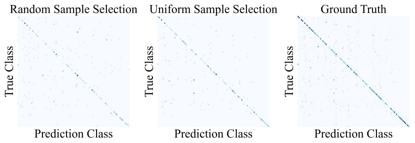
Figure 3: Ablation study on transition matrix estimation by comparing our method with random sampling and ground truth.

To validate the performance of transition matrix estimation, we compare our confidence-based uniform sampling strategy to a random sampling baseline. The result on the ImageNet-V dataset is shown in Figure 3. To quantitatively show the superiority of our method, we compute the $\ell_{2}$ norm of the difference between one estimation and the ground truth which indicates the fidelity of the estimation. As a result, our estimation is much more accurate by achieving $3.83$ norm, compared to $4.46$ of random sampling.

Table 3: Performance comparison between choosing noisy classes through transition matrix (MVT) and using Top-$N$ predictions.

	IN-A	IN-SK	IN-Val	IN-R	IN-V2	IN-V
Top-$N$ Pred.	60.3	58.4	74.2	85.3	67.7	58.3
MVT	65.5	59.0	75.1	86.0	70.7	61.6

Ablation Study on Choosing Noisy Classes

Further, we justify the choice of using a transition matrix to obtain the noisy classes. As a comparison, we use the top-$6$ predictions as the therapy candidates and show the results in Table LABEL:tab:4. We can see on all datasets, our method can outperform the opponent with non-trivial improvements. Therefore, leveraging the transition matrix to find the potential noisy classes is more effective than using prediction.

Ablation Study on Detection Score

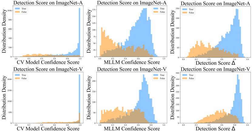
Figure 4: Ablation study on detection score distribution. Upper: ImageNet-A; Lower: ImageNet-V.

To analyze the proposed detection score on conducting diagnosing, we show the distribution of prediction confidence provided by the vision model, MLLM, and our detection score $\Delta$ in Figure 4. Based on the results, we can justify our design of $\Delta$: In the left column, we can see the confidence of correctly classified examples is very high, but the wrong ones show uniform distribution. Conversely, in the middle column, although MLLM poses slightly lower scores on correct ones, it significantly suppresses the confidence of wrong ones. As a result, we combine two scores to obtain $\Delta$, which can produce clearly separable distributions to benefit the diagnosing process. Unless specified, we set the threshold $\delta=0.6$ which works effectively in most scenarios.

Table 4: Comparison of classification accuracy (%) on 5 OOD datasets with different MLLMs. We compare the performance of our method on CLIP ViT-L [54] models with two different MLLM backbones, including Otter [39] and MMICL [75]. Our method is applicable to different MLLMs with ICL ability.

MLLM	Method	IN-A	IN-R	IN-SK	IN-V	iWildCam
None	CLIP [54]	69.3	86.6	59.4	51.8	13.4
Otter [39]	MVT	64.1	85.2	59.5	51.9	16.2
	+FT	73.5	88.7	60.0	55.7	-
MMICL  [75]	MVT	71.2	88.1	59.0	62.1	25.0
	+FT	75.1	89.5	61.4	68.8	-

Ablation Study on MLLM Backbone

To testify the effectiveness of MVT on different MLLM backbones, here we instantiate our method using Otter [38] and compare it to the previous realization on MIMIC [75]. The result is shown in Table 4. We can see that both the implementation on MMICL and Otter show superior performance to the employed vision encoder backbone. Although the performance slightly differs between Otter and MMICL, which could be due to the model capacity and their training strategy, we can generally conclude that our MVT method is applicable to different MLLMs backbones with ICL and could further benefit from more sophisticated MLLMs in the future.

3.4 Performance Analysis

Further, we conduct qualitative analysis to thoroughly validate the effectiveness of our MVT.

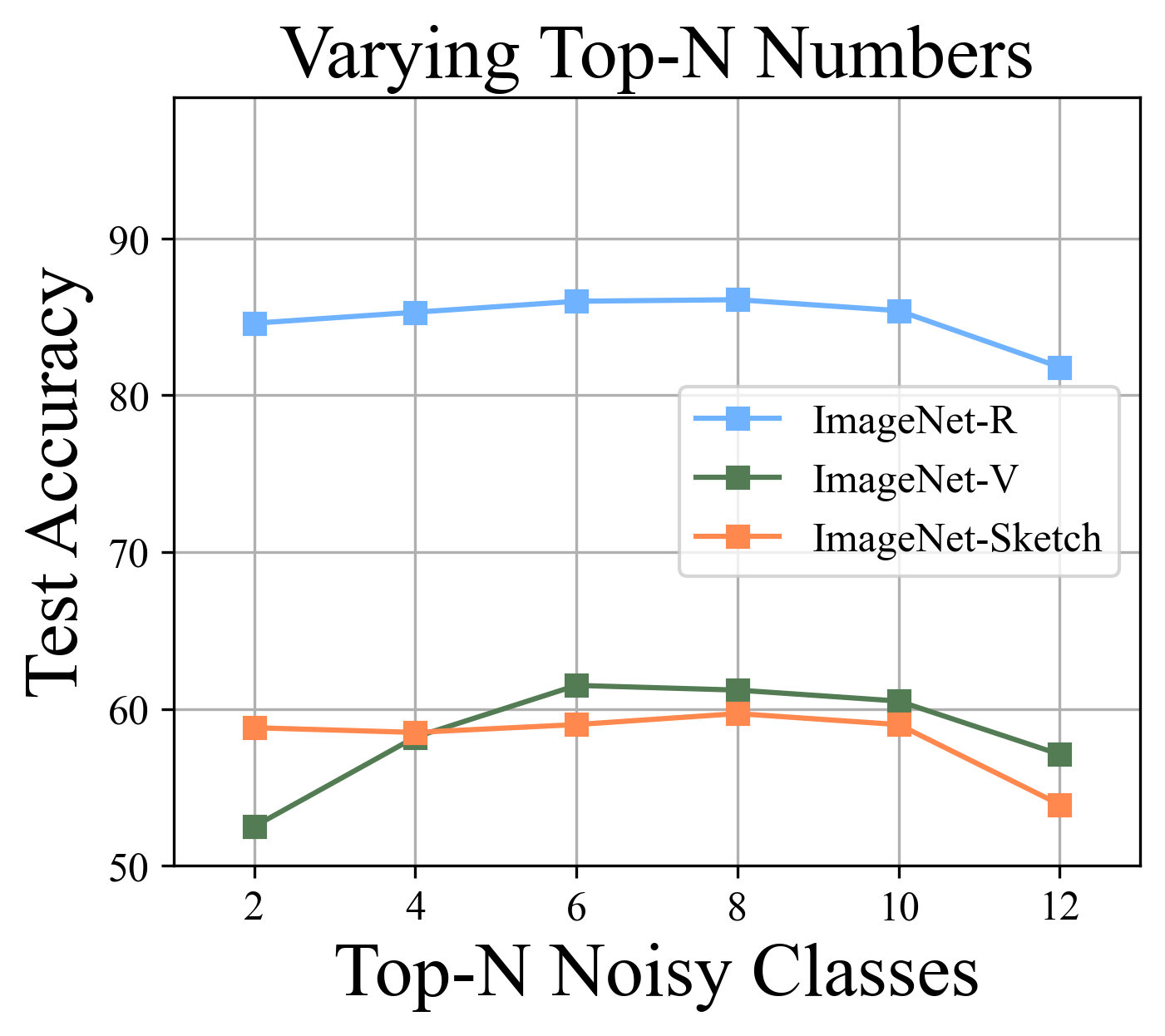
Figure 5: Performance analysis by varying the number of top-$N$ chosen noisy classes.

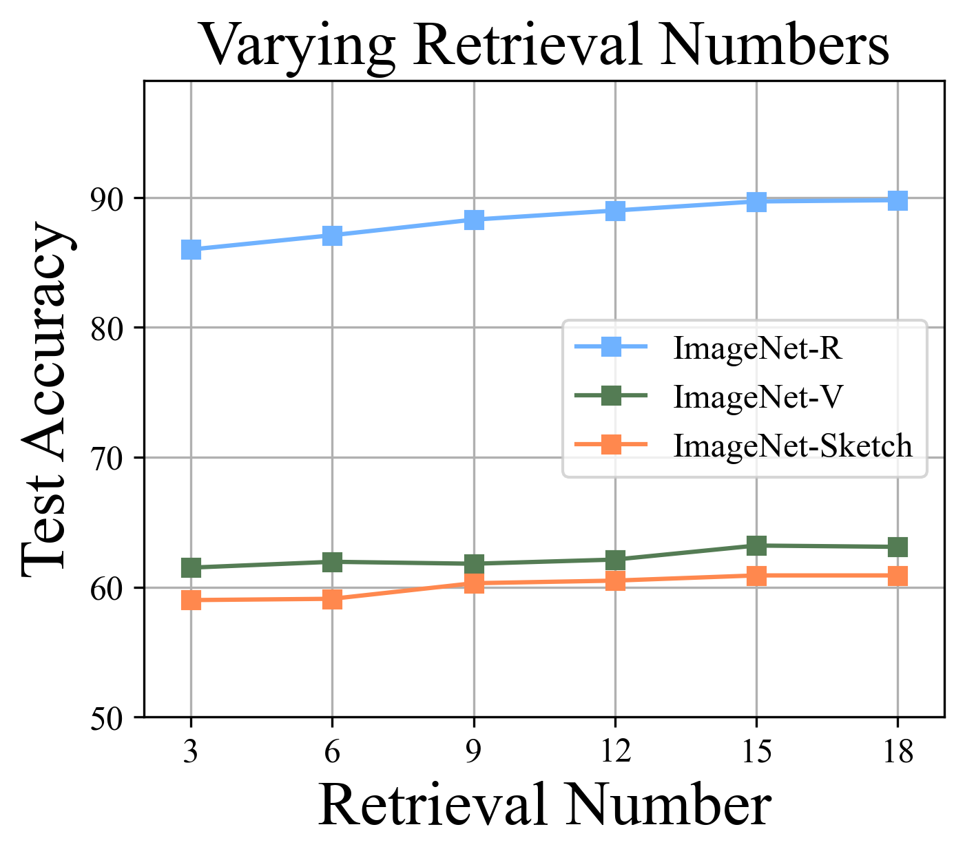
Figure 6: Performance analysis by varying the number of retrieved exemplars.

Choice of Top-$N$ Noisy Classes

To study how a varied number of chosen noisy classes could affect the performance of our method, we change the top-$N$ number from $2$ to $12$, and show the result on ImageNet-R, ImageNet-V, and ImageNet-Sketch datasets in Figure 6. We find a common phenomenon that either too small or too large a number of $N$ could hurt the performance. This could be because that small $N$ would ignore too many potential ground-truth classes. In contrast, large $N$ includes too many choices that could interfere with the final prediction. Setting $N$ to $6$ could be an ideal choice for ImageNet-based datasets.

Effect of Retrieval Numbers

In our experiments, we retrieve exemplars for $3$ times and average the predictions. To further investigate the effect of varied retrieval numbers, we change the number of retrievals from $3$ to $18$ and conduct experiments on the same OOD datasets as above. Specifically, we consider one positive and negative pair for a single DICL round as one retrieval. We repeat this process for $R$ times and ensemble the MLLM predictions through $\frac{1}{R}\sum_{r}^{R}\left[h_{c}^{true,r},h_{c}^{false,r}\right]$. In this way, it is possible that MLLM predictions would be more accurate. The result is shown in Figure 6. We observe that the performance steadily improves as the retrieval number increases, however, the performance gains vanish when the retrieval number becomes too large. Moreover, large retrieval numbers would multiply the computation cost. Therefore, it is suggested to set the number to a reasonably small value.

Performance of Different Retrieval Strategy

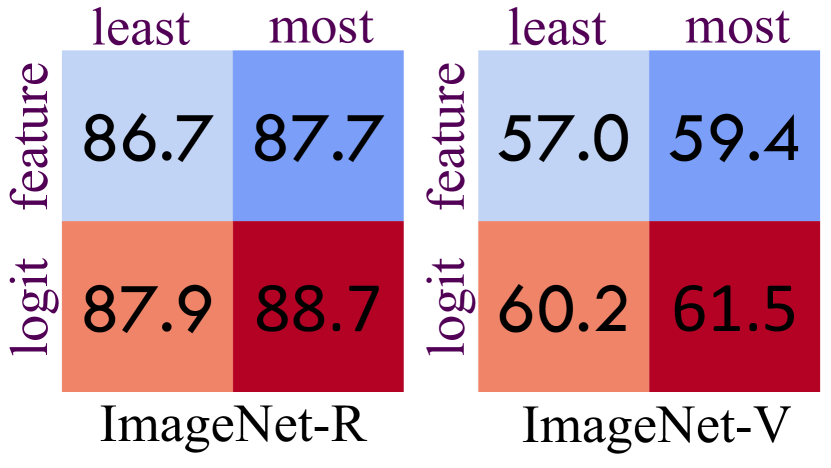
Figure 7: Performance analysis on different retrieval strategies.

As shown by Alayrac et al. [1], Retrieval-based In-Context Example Selection (RICES) could significantly influence the performance of ICL. Therefore, here we carefully investigate its influence in our problem setting. Specifically, we propose two retrieval strategies, namely feature-based retrieval and logit-based retrieval. The former one is based on feature similarity and the latter one is based on the prediction logit. For each strategy, we conduct experiments on selecting the most similar examples and the least similar examples, which are denoted as “most” and “least”, respectively. The results are shown in Figure 7. Apart from the intuitive finding that least-similar retrieval is inferior to selecting the most similar examples, we also observe that logit-based retrieval is more effective than feature-based one. We assume this is due to the intended task being image classification which is more related to the prediction logit rather than feature similarity.

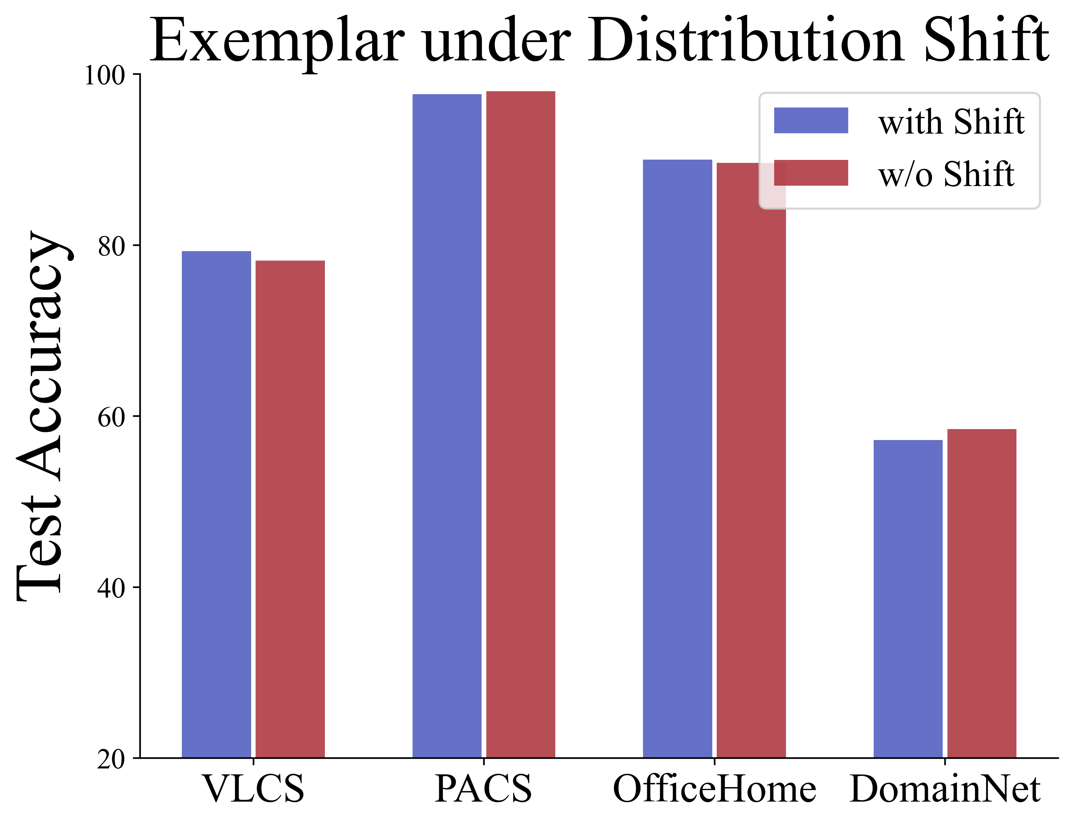
Figure 8: Performance analysis on in-context exemplars with distribution shift.

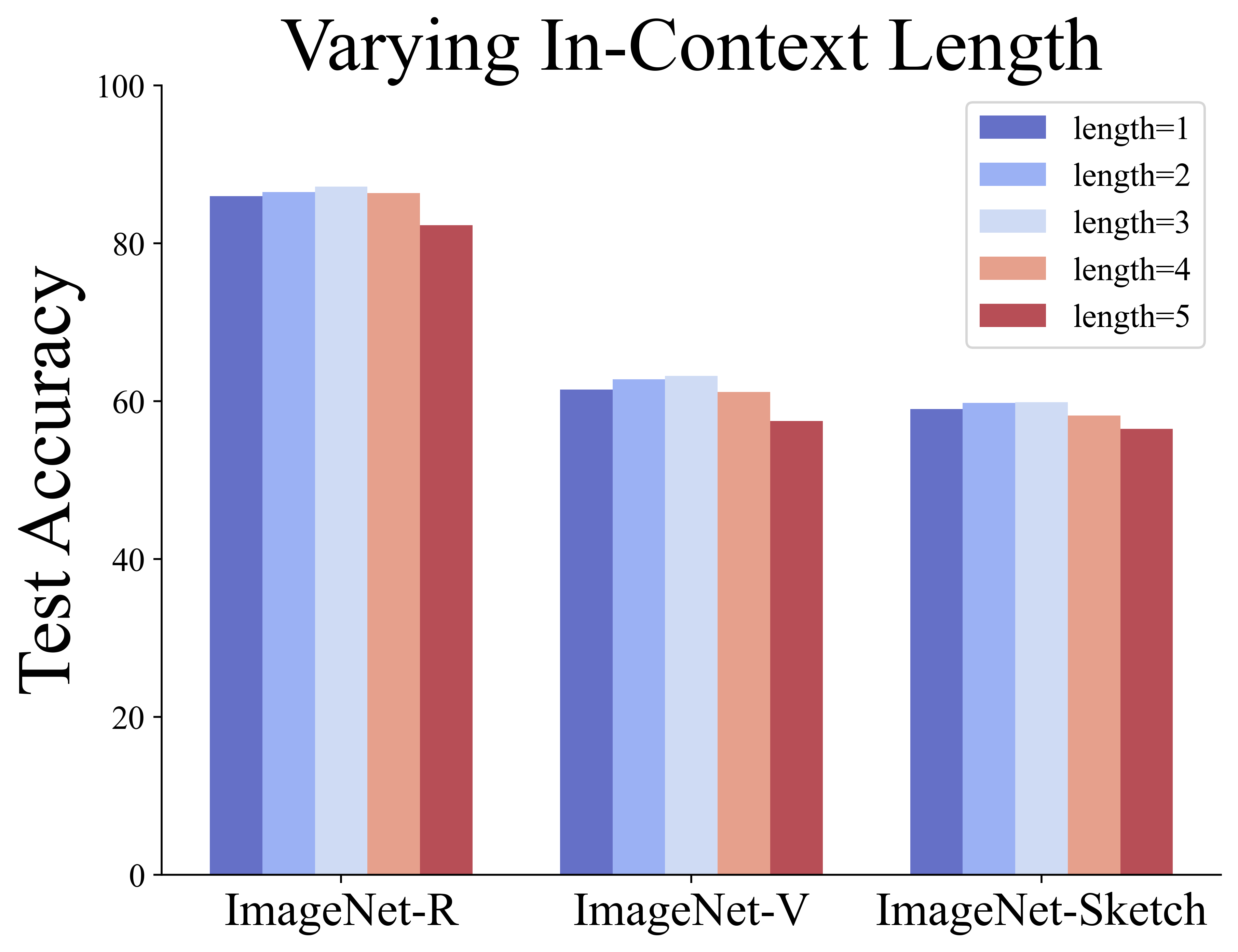
Figure 9: Performance analysis by varying the length of in-context exemplars.

Effect of In-Context Exemplars with Distribution Shift

When the support set suffers from a distribution shift from the target OOD dataset, whether DICL can still perform robustly remains to be validated. Hence, we leave one domain out as our support set and leveraging the rest domains as our target OOD dataset. In comparison, we choose a small hold-out data split as the support set which shares the same distribution as the OOD dataset. The results are shown in Figure 9. Surprisingly, we find that the performance is not influenced by the distribution shift, which demonstrates that our MVT can still be effective when exemplars are retrieved from different distributions.

Effect of Varying In-Context Length

Furthermore, we analyze the effect of increasing the exemplar length during each inference. Particularly, we consider one positive and negative exemplar pair as length $1$. Here we vary the length from $1$ to $5$ and show the results in Figure 9. We observe slight improvement when the length gradually increases which is consistent with the theoretical finding [67] that increasing the number of exemplars leads to improved performance. However, when the length is longer than $4$ the performance drops and the predictions of MLLM become unstable which could be other than “True” or “False”. This could be due to the capacity of MLLMs to handle a limited amount of information, which is worth conducting further studies on sophisticated MLLMs in the future.

Figure 10: OOD detection analysis. Upper: Detection score distribution on ImageNet-A; Lower: F1 scores of vision model confidence, MLLM diagnosing confidence, and our $\Delta$ score in ImageNet-A, ImageNet-R, and ImageNet-V.

Performance of OOD Detection

At last, we consider a more challenging scenario where data from open classes could exist in the target dataset. Here we simulate this situation by choosing $60\%$ of the classes as closed classes and the rest are open classes. To detect such open-class data, i.e., OOD detection [24], we use the vision model prediction confidence as a baseline and compare with the MLLM diagnosing confidence as well as the detection score $\Delta$ in Eq. 3. The result is shown in Figure 10. In the upper row, we observe the similar clearly distinguishable distributions using our score $\Delta$ as in Figure 4. In the lower row, we show the F1 score of each detection criterion under a threshold varied from $0$ to $1$ on three datasets. When a criterion produces confidence larger than the threshold, it would predict as close-class data, other as open-class ones. Based on the result, we find that MLLM achieves better detection performance when the threshold is small, but vision model confidence is relatively better when the threshold is large, i.e., MLLM can effectively detect open classes while vision models are better at recognizing close classes. However, an effective detection should have a reasonable threshold value that is neither too large nor too small and meanwhile has a high F1 score. Hence, by combining them together, our detection score $\Delta$ can achieve the best F1 score when the threshold is around the middle range.

4 Conclusion

In this paper, we propose a novel paradigm of fine-tuning vision models via leveraging MLLMs to improve visual robustness on downstream OOD tasks. Specifically, we effectively estimate a transition matrix to help find the most probable noisy classes. By using a positive exemplar and a negative exemplar retrieved based on the noisy classes, we can conduct DICL to rectify incorrect vision model predictions through two stages dubbed diagnosing and therapy. Thanks to the rectified predictions, the robustness of vision models can be further improved through fine-tuning. We conduct extensive quantitative and qualitative experiments to carefully validate the effectiveness of our method. Our framework can significantly reduce the cost of training vision models and provide insights into many visual recognition problems such as OOD detection, OOD generalization, weakly-supervised learning, etc.

 

Supplementary Material for
“Machine Vision Therapy: Multimodal Large Language Models
Can Enhance Visual Robustness via Denoising In-Context Learning”  

Index

1. 1 Introduction
2. 2 Methodology
   1. 2.1 Problem Formulation and Overview
   2. 2.2 Transition Matrix Estimation
   3. 2.3 Denoising In-Context Learning
   4. 2.4 Fine-Tuning of Vision Models
3. 3 Experiments
   1. 3.1 Experiments Setup
      1. 3.1.1 Datasets and Models
      2. 3.1.2 Evaluation Settings
   2. 3.2 Quantitative Comparison
   3. 3.3 Ablation Study
   4. 3.4 Performance Analysis
4. 4 Conclusion
5. A Related Work
   1. A.1 OOD Generalization
   2. A.2 Multimodal Large Language Models
6. B Additional Details
7. C Additional Quantitative Comparisons
   1. C.1 Quantitative Comparison using Otter
   2. C.2 MVT on Additional Vision Models
   3. C.3 Robustness against Visual Corruptions
   4. C.4 Robustness against Spurious Correlation
   5. C.5 Performance on Recognizing Fine-grained Attributes
8. D Additional Performance Analysis
   1. D.1 Analysis on MLLM Guided Fine-Tuning
   2. D.2 Analysis on Various DICL Designs
   3. D.3 Analysis on OOD Robustness
   4. D.4 Analysis on OOD Detection
9. E Limitation and Broader Impact

In this supplementary material, we provide extensive quantitative and qualitative studies on a wide range of datasets to thoroughly understand the essence of the proposed framework. First, we discuss some related works regarding OOD generalization and Multimodal Large Language Models in Section A. Then, we elucidate the additional details of our experimental setting and implementation in Section B. Further, we provide additional quantitative comparisons on different MLLM and CV backbone models, and different OOD types in Section C. Finally, we perform additional analysis to further explore the effectiveness of our method in Section D. In the end, we discuss the limitation of this work and broader impact in Section E

Appendix A Related Work

In this section, we provide a brief discussion of OOD generalization problem and multi-modal large language models.

A.1 OOD Generalization

OOD data refers to those with different distributions from training data. OOD generalization aims at improving the performance of deep models to unseen test environments. Researchers attempted to tackle the problem from different perspectives, such as data augmentation, OOD detection, invariant causal mechanisms, and so on. Data augmentation is effective in improving model generalization. Typical methods involve Cutout [10], which randomly occludes parts of an input image; CutMix [70], which replaces a part of the target image with a different image; Mixup [73], which produces a convex combination of two images; DeepAugment [26], which passes a clean image through an image-to-image network and introduces several perturbations during the forward pass. Some methods conduct OOD detection to separate OOD data. Typical methods include softmax confidence score [24], which is a baseline for OOD detection; Outlier Exposure (OE) [25], which uses unlabeled data as auxiliary OOD training data. Energy scores are shown to be better for distinguishing OOD samples from IID ones [46]. Some work resort to causality to study the OOD generalization problem. Typical methods include MatchDG [50], which proposes matching-based algorithms when base objects are observed and approximate the objective when objects are not observed; INVRAT [4], which leveraged some conditional independence relationships induced by the common causal mechanism assumption.

A.2 Multimodal Large Language Models

The field of vision-language models has witnessed significant advancements in recent years, driven by the growing synergy between computer vision and natural language processing. Notably, this synergy has led to the exceptional zero-shot performance of CLIP [54], a model that employs a two-tower contrastive pre-training approach to align image and text information. In the rapidly evolving landscape of LLMs, exemplified by GPTs [3], LLaMA [59], and Vicuna [6], it has become evident that LLMs possess the capacity to process information from diverse domains. BLIP-2 [41], for instance, serves as a foundational model, aligning visual features and text features using a Querying Transformer (Q-former) and utilizing OPT [74] and FLAN [7] as language models. Building upon BLIP-2, Instruct-BLIP [8] has enhanced instruction-following capabilities. To further bolster the instruction-following proficiency of multi-modal models, LLaVA [44] and Mini-GPT4 [77] have introduced meticulously constructed instruction sets, which have found widespread application in various multi-modal models. mPLUG-Owl [69] introduces a two-stage learning paradigm, first fine-tuning the visual encoder and then refining the language model with LoRA [28]. This approach effectively fuses image and text features. Some models consider additional modalities, such as ImageBind [17], which simultaneously incorporates data from six modalities without the need for explicit supervision, and PandaGPT [58] which enhances its instruction-following capabilities. Several multi-modal models prioritize the in-context learning abilities of LLMs. Flamingo [1], in one of the pioneering efforts, integrates a gated cross-attention module to align the image and text spaces. Otter [39] refines OpenFlamingo [2], an open-source version of Flamingo, by introducing instruction-tuning datasets to improve instruction-following abilities. Multi-Modal In-Context Learning (MMICL) [75] is a comprehensive vision-language model that incorporates Instruct-BLIP, enabling the analysis and comprehension of multiple images, as well as the execution of instructions. MLLMs possess the remarkable capacity to capture intricate details and engage in reasoning when presented with an image. Nevertheless, it remains uncertain about how to enhance visual perception by harnessing the knowledge embedded within LLMs.

Appendix B Additional Details

We run all our experiments on 8 NVIDIA 3090 GPUs using the Pytorch framework. During MVT, we freeze the MLLM backbone model to stop generating gradients that might cause additional computational costs. Then, for the vision encoder, we use model.eval() for producing vision predictions. Further, the predictions are evaluated and corrected. Based on the rectified predictions, we use torch.optim.Adam() or torch.optim.SGD() optimizer to fine-tune the vision model for $3$ epochs. Note that we conduct fair comparisons in each experiment by using the same optimizer. Due to the memory requirement of ViT-g is large, thus we use torch.optim.SGD() to optimize ViT-g model and torch.optim.Adam() for other vision models. The vision encoder is trained with torch.float32 precision to prevent overflow. The batch size for ViT-L vision encoder is 16 and the batch size for ViT-g is $8$ with $2$ accumulation steps. The learning rate of the training process is $5e-7$ and cosine scheduler for ViT-L with torch.optim.Adam(). Due to limited GPU memory, we fine-tune ViT-g with torch.optim.SGD() of learning rate $1e-4$ and $0$ momentum. Besides, experiments in Sec. C.2 in Appendix does not follow the settings mentioned above. Because the vision encoders to be fine-tuned have large capacity gap with the vision encoders in MLLMs. We need to fine-tune the vision encoder to match the performance of MLLMs. Therefore, the learning rate is adjusted to $1e-4$ and the training epoch is adjusted to $20$. Note that all the fine-tuned data from the evaluation dataset are the chosen ones for therapy. Then we test the performance of all baseline methods on a split-out test set.

In DICL, our prompt for multi-class classification tasks is as follows:

where the {replace_token} is further replaced by the image feature, and $<$#text$>$ is further replaced by the class name. The MMICL and Otter model we use can be found at https://github.com/haozhezhao/mic and https://github.com/Luodian/Otter, respectively. All our fine-tuned vision models can be directly found in Openai CLIP models: https://huggingface.co/openai.

Appendix C Additional Quantitative Comparisons

Here we provide extensive quantitative comparisons of different MLLM and vision models, in various robustness settings.

C.1 Quantitative Comparison using Otter

First, similar to Table 1 in the main paper, here we conduct additional experiments on various ImageNet-based datasets and DomainBed datasets using ViT-L but a different MLLM backbone: Otter [39]. The results are shown in Tables 5 and 6. We find that the performance of MVT is dependent on the MLLM backbone: when using Otter as the backbone model for MVT, the OOD performance would slightly degrade from the performance of MMICL, which could be due to the capability of MLLM to conduct ICL. However, the rectified predictions can still contain useful information to boost the performance of vision models. In several cases in ImageNet-Val, MNIST, and ImageNet-R, Otter with fine-tuning can still improve the visual robustness to the best or second-best results.

Table 5: Classification accuracy (%) of baseline CLIP models and our method with MMICL [75] and Otter [39] as the VLMs on 5 ID datasets and 5 OOD datasets. We compare the performance of our method, and the fine-tuned models supervised by our method with the baseline models, i.e., ViT-L from CLIP [54]. Fine-tuning with both MMICL and Otter improves the classification accuracy.

MLLM	Method	ID					OOD
		IN-Val	IN-V2	Cifar10	Cifar100	MNIST	IN-A	IN-R	IN-SK	IN-V	iWildCam
None	CLIP [54]	75.8	70.2	95.6	78.2	76.4	69.3	86.6	59.4	51.8	13.4
MMICL  [75]	MVT	75.2	70.8	97.9	78.9	53.0	71.2	88.1	59.0	62.1	25.0
	+FT	76.9	70.5	96.7	82.0	79.2	75.1	89.5	61.4	68.8	-
Otter [39]	MVT	74.2	67.4	94.7	70.1	52.0	64.1	85.2	59.5	51.9	16.2
	+FT	76.3	70.1	96.6	81.8	81.3	73.5	88.7	60.0	55.7	-

Table 6: Classification accuracy (%) of baseline CLIP models and our method with MMICL [75] and Otter [39] as the VLMs on 4 subsets of DomainBed datasets, including VLCS, PACS, OfficeHome, and DomainNet. We compare the performance of our method and the fine-tuned models supervised by our method with the baseline models, i.e., ViT-L from CLIP [54]. Fine-tuning with both MMICL and Otter improves the classification accuracy.

MLLM	Datasets	VLCS				PACS				OfficeHome				DomainNet					Avg
	method	0	1	2	3	0	1	2	3	0	1	2	3	0	1	2	3	4
None	CLIP [54]	74.9	83.5	80.3	74.5	97.8	97.4	97.5	99.4	87.7	92.7	85.7	85.6	61.1	62.1	60.2	78.4	51.1	80.6
MMICL  [75]	MVT	83.8	89.0	87.2	80.3	97.6	97.5	98.0	99.4	87.7	93.4	89.0	88.5	61.3	62.1	60.4	78.7	53.4	82.8
	+FT	84.2	89.8	87.9	82.5	98.0	98.2	98.0	99.8	90.9	95.0	90.9	90.8	62.5	63.8	62.4	80.1	54.0	84.0
Otter  [39]	MVT	67.5	77.4	73.7	66.6	97.0	96.3	96.5	99.0	85.6	89.9	83.6	83.3	56.5	58.6	56.3	74.1	46.5	77.0
	+FT	76.8	87.7	82.3	77.4	98.0	97.7	98.0	99.8	88.7	93.4	87.7	87.1	62.0	63.0	61.3	79.7	53.4	82.0

C.2 MVT on Additional Vision Models

Then, we conduct MVT using MMICL but using different vision backbone models such as ViT-B and ResNet-50 on ImageNet and DomainBed datasets. The results are shown in Tables 7 and 8. We can see that the performance of MVT is quite strong compared to other vision models which shows over $10\%$ and $4\%$ improvements in ImageNet datasets and DomainBed datasets, respectively. Especially on ImageNet-V2, ImageNet-A, ImageNet-R, and ImageNet-V, the performance improvement of MVT are encouragingly over $15\%$, $24\%$, $12\%$, and $23\%$, respectively. After fine-tuning, the performance can be improved in most cases, such as ResNet-50 is further improved by $13.1\%$ and $3.3\%$ correspondingly on ImageNet-V2 and DomainBed thanks to MMICL.

Table 7: Classification accuracy (%) of baseline CLIP models and our method on 5 ID datasets and 5 OOD datasets. We compare the performance of our method, and the fine-tuned models supervised by our method with the baseline models, including ResNet-50 and ViT-B/32. The chosen MLLM is MMICL [75].

Arch	Method	ID					OOD
		IN-Val	IN-V2	Cifar10	Cifar100	MNIST	IN-A	IN-R	IN-SK	IN-V	iWildCam
RN50	CLIP [54]	59.7	52.6	71.5	41.9	58.5	23.9	60.7	35.4	31.1	8.2
	MVT	76.2	70.8	80.2	49.7	50.8	47.5	72.9	41.6	54.1	14.5
	+FT	66.3	65.7	75.1	46.9	47.3	32.1	64.4	36.5	38.2	-
ViT-B	CLIP [54]	62.9	56.1	89.9	65.0	47.9	32.2	67.9	41.9	30.5	10.9
	MVT	77.5	71.0	92.5	60.4	51.5	60.6	83.0	47.8	53.1	19.3
	+FT	66.3	66.0	90.1	59.5	46.6	38.8	68.7	43.1	37.6	-

Table 8: Classification accuracy (%) of baseline CLIP models and our method on 4 subsets of DomainBed datasets, including VLCS, PACS, OfficeHome, and DomainNet. We compare the performance of our method and the fine-tuned models supervised by our method with the baseline models, including ResNet-50 and ViT-B/32. The chosen MLLM is MMICL [75].

Arch	Datasets	VLCS				PACS				OfficeHome				DomainNet					Avg
	method	0	1	2	3	0	1	2	3	0	1	2	3	0	1	2	3	4
RN50	CLIP [54]	75.0	82.3	81.3	75.0	91.3	90.3	90.0	96.2	71.7	80.9	69.4	67.8	47.2	46.8	44.9	64.0	32.9	71.0
	MVT	84.3	88.0	88.7	81.8	96.0	96.1	95.4	98.8	77.2	85.3	77.5	75.4	46.1	46.3	43.4	61.7	33.2	75.0
	+FT	83.7	87.3	88.1	81.3	95.6	95.7	95.1	98.6	75.9	85.0	75.8	74.7	45.3	45.6	43.0	60.4	32.6	74.3
ViT-B	CLIP [54]	74.0	82.0	79.6	74.4	93.6	92.8	93.0	98.2	79.2	86.4	77.4	76.3	49.7	54.3	51.0	68.7	40.7	74.8
	MVT	84.2	87.3	88.4	82.8	96.7	96.4	96.6	98.8	84.0	89.3	82.9	81.5	49.5	53.1	51.5	69.9	41.7	78.5
	+FT	76.0	84.8	81.3	81.6	92.9	88.8	89.4	93.3	81.1	88.3	80.8	77.7	47.2	52.5	48.7	66.9	40.5	74.8

Table 9: Classification accuracy (%) of baseline CLIP models and our method with MMICL [75] as the VLM on 15 corruptions and 5 severities of ImageNet-C datasets. We compare the performance of our method and the fine-tuned models supervised by our method with the baseline models, i.e., ViT-L from CLIP [54]. The fine-tuned models with our MVT method have the best performance.

Arch.	Datasets	Gaussian Noise						Shot Noise						Impulse Noise
	method	1	2	3	4	5	avg	1	2	3	4	5	avg	1	2	3	4	5	avg
MMICL [75]	CLIP [54]	69.8	66.7	59.7	46.9	30.6	54.7	70.5	64.9	57.7	43.6	32.1	53.8	65.7	60.2	55.9	45.0	32.7	51.9
	MVT	70.1	67.5	61.2	49.8	33.6	56.4	70.8	66.8	59.2	46.1	35.6	55.7	66.3	61.9	58.4	47.5	35.6	53.9
	+FT	71.0	67.9	61.3	48.7	33.5	56.5	72.0	67.1	60.1	46.1	35.2	56.1	68.5	64.2	59.8	48.9	35.8	55.4
		Defocus Blur						Glass Blur						Motion Blur
		1	2	3	4	5	avg	1	2	3	4	5	avg	1	2	3	4	5	avg
	CLIP [54]	66.1	62.4	53.0	43.4	35.0	52.0	65.5	59.3	40.5	33.8	25.4	44.9	70.9	66.8	59.9	49.5	41.8	57.8
	MVT	67.1	63.3	55.8	47.6	38.8	54.5	67.1	61.3	42.8	36.0	29.4	47.3	71.9	67.7	60.9	51.5	43.2	59.0
	+FT	68.8	64.1	56.3	47.4	38.4	55.0	68.9	64.8	45.2	37.6	30.2	49.3	72.8	69.1	62.1	52.7	45.3	60.4
		Zoom Blur						Snow						Frost
		1	2	3	4	5	avg	1	2	3	4	5	avg	1	2	3	4	5	avg
	CLIP [54]	62.2	55.9	49.8	43.9	37.3	49.8	68.3	61.2	61.9	56.1	52.6	60.0	68.5	61.2	53.8	51.1	46.6	56.2
	MVT	64.1	57.3	52.0	45.7	38.7	51.6	69.2	61.5	62.9	57.1	54.0	60.9	69.5	61.5	54.2	52.7	47.4	57.1
	+FT	65.2	59.2	54.2	48.8	41.4	53.8	70.6	63.9	64.6	59.2	55.6	62.8	71.9	65.2	57.9	56.4	51.5	60.6
		Fog						Brightness						Contrast
		1	2	3	4	5	avg	1	2	3	4	5	avg	1	2	3	4	5	avg
	CLIP [54]	69.8	67.9	65.0	61.3	52.0	63.2	74.3	74.0	72.8	70.6	68.1	72.0	70.6	69.3	64.8	52.4	35.1	58.4
	MVT	70.7	69.2	66.5	62.6	53.8	64.6	74.7	74.1	72.6	71.1	68.8	72.3	70.9	69.9	65.1	52.9	36.9	59.1
	+FT	72.5	71.3	69.5	67.1	60.3	68.1	76.0	75.1	74.3	73.1	71.1	73.9	73.5	73.5	70.2	59.2	42.7	63.8
		Elastic						Pixelate						JPEG
		1	2	3	4	5	avg	1	2	3	4	5	avg	1	2	3	4	5	avg
	CLIP [54]	69.2	50.6	64.1	53.1	30.4	53.5	71.0	70.4	66.2	60.1	54.6	64.5	70.8	67.7	65.1	58.0	45.3	61.4
	MVT	70.0	51.1	65.8	55.2	32.7	55.0	71.7	70.7	66.5	61.9	57.3	65.6	72.5	69.6	67.5	60.5	47.7	63.6
	+FT	70.7	53.6	67.7	58.5	32.2	56.5	72.8	71.8	69.1	62.9	57.7	66.9	71.2	68.9	65.8	60.0	48.8	62.9

C.3 Robustness against Visual Corruptions

Further, we consider the visual robustness against image corruptions by evaluating our method on a robustness benchmark: ImageNet-C [23]. Specifically, there are 15 different types of corruption with different corruption severities varied from 1 to 5. Here we cover all scenarios to evaluate our method using MMICL as a backbone model and a baseline method CLIP ViT-L. The results are shown in Table 9. We can see that our method shows very strong performance in all scenarios. Compared to CLIP, using MVT can improve the performance by over $2\%$, and through fine-tuning, the performance is further boosted by over $4\%$. The encouraging results once again demonstrate the effectiveness of our method.

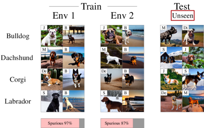
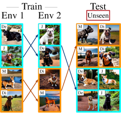
Figure 11: Figures are from Lynch et al. [49], the letters on each images denote a certain background. There are two spurious correlation types in the Spawrious dataset, namely O2O and M2M. In the O2O setting on the left, each dog class is correlated to one certain background type and different distribution has different correlation probability as shown by the bar below the O2O figure. As for the M2M setting on the right, multiple classes and backgrounds are correlated together and the correlation changes to different groups of classes and backgrounds during testing.

Table 10: Performance comparison between MVT and CLIP on robustness against spurious correlation using Spawrious dataset.

Type	O2O_easy	O2O_medium	O2O_hard	M2M_easy	M2M_medium	M2M_hard	Avg.
ViT-L	94.1	95.4	93.3	96.7	95.0	92.5	94.5
MVT	95.8	96.3	93.6	96.8	95.8	92.9	95.2
ViT-g	94.6	97.0	92.6	96.7	95.6	94.8	95.2
MVT	95.3	97.4	92.8	96.8	96.6	95.4	95.7

C.4 Robustness against Spurious Correlation

Moreover, we consider a common distribution shift scenario where the training dataset and test dataset have different foreground and background correlation, i.e., spurious correlation. Specifically, as shown in Figure 11 standing for the Spawrious dataset that we use, there are two different settings: One-To-One (O2O) correlation where each class is correlated to one background type with a certain probability. The foreground objects in the training dataset and test dataset have different probabilities to be combined with a certain background. For the Many-To-Many (M2M) setting, the foregrounds and backgrounds are split into subgroups that contain multiple classes and background types. When different subgroups are correlated together between training and test datasets, the M2M spurious correlation is formed and brings more complexity. In the Spawrious dataset, there are three levels of hardness based on correlation probability difference between training and test datasets, namely easy, medium, and hard. Here we consider all scenarios and show the results in Table 10. We can see that the MVT method can outperform the ViT-L and ViT-g baseline methods in all scenarios, which leads to the conclusion that our method is robust to spurious correlations and can identify the class-of-interests despite the changing backgrounds.

C.5 Performance on Recognizing Fine-grained Attributes

Figure 12: Examples of celebA photos with different attributes.

Additionally, here we further explore the capability of recognizing subtle attributes based on the CelebA dataset [48]. Particularly, we consider 12 face attributes, as shown in Figure 12. For each attribute, we testify whether a learning model could correctly identify the attribute in a given image. Here we compare our MVT method with CLIP ViT-L and ViT-g, and the performance of MVT produced by conducting therapy on ViT-L and ViT-g models.

Table 11: Class names of 12 chosen attributes.

Attribute	-1	+1
Male	a woman	a man
Wear_Hat	not wearing a hat	wearing a hat
Smiling	not smiling	smiling
Eyeglasses	not wearing eye glasses	wearing eye glasses
Blond_Hair	not having blond hair	having blind hair
Mustache	not having mustache	having mustache
Attractive	not attractive	attractive
Wearing_Lipstick	not wearing lipstick	wearing lipstick
Wearing_Necklace	not wearing necklace	wearing necklace
Wearing_Necktie	not wearing necktie	wearing necktie
Young	not young	young
Bald	not bald	bald

Particularly, since CelebA is a binary classification task, here we design different prompts for vision models and our MLLM. For CLIP models, we use The person in this image is $<$#classname$>$ as text input, where $<$#classname$>$ of each attribute is shown in Table 11. For our method, we still designed one positive prompt and one negative prompt for each ICL round. Specifically, for “Male” attribute, our in-context instruction is as follows:

in which is first exemplar demonstrates an image of a male positively described as male, the second exemplar shows an image of a male negatively described as female, and finally, we ask whether the input image is a male and use the output of MLLM as the prediction.

Table 12: Performance comparison between MVT and CLIP on recognizing fine-grained attributes using CelebA dataset.

Attr.	Male	Wearing_Hat	Smiling	Eyeglasses	Blond_Hair	Mustache	Attractive	Wearing_Lipstick	Wearing_Necklace	Wearing_Necktie	Young	Bald	Avg.
ViT-L	63.0	60.8	64.5	75.8	36.2	29.0	42.0	30.8	38.0	37.5	66.6	86.3	52.5
MVT	74.0	67.0	65.4	76.1	53.0	55.8	42.4	39.4	38.6	53.9	73.5	88.1	60.6
ViT-g	98.5	75.5	70.4	83.8	46.0	66.6	58.2	72.5	43.5	28.4	54.1	91.3	65.7
MVT	98.9	77.2	71.0	84.1	58.3	74.9	59.0	73.2	43.6	41.2	56.1	91.8	69.1

The results on CelebA are shown in Table 12, we observe that our method is quite effective in recognizing fine-grained attributes and its performance significantly surpasses ViT-L and ViT-g with a large margin. Especially in attributes such as “Blond_Hair”, “Mustache”, and “Wearing_Necktie”, the performance improvements are even over $10\%$ on both two CLIP models, and the final averaged results on all 12 attributes, the total improvements are $8.1\%$ and $3.4\%$ for ViT-L and ViT-g, respectively. Therefore, it is reasonable to conclude that our method can be effectively conducted on fine-grained attribute recognition and significantly outperforms several powerful vision models.

Appendix D Additional Performance Analysis

In this section, we carefully conduct additional performance analysis to further validate the effectiveness of our MVT.

D.1 Analysis on MLLM Guided Fine-Tuning

We find that our MLLM-guided fine-tuning is quite effective in further improving the prediction accuracy based on MVT corrections. To investigate why such a fine-tuning process can help the learning performance, here we compare the prediction logits of image examples from ImageNet and its variant datasets before and after the fine-tuning process. As we already shown in Figure 4 in the main paper, our MVT framework can effectively find the examples misclassified by the vision model, thus we randomly select some images that are further processed with our therapy and fine-tuning. The logits are shown in Figures 13 and 14, we can observe that after fine-tuning, the predictions of the previously incorrect examples are finally rectified which shows that the proposed MVT method is indeed helpful for visual recognition. Moreover, we also observe that the ground truth logit values of some examples are quite small which means that the vision models are very confident in their incorrect predictions. Thanks to our MVT, we can not only successfully find the ground truth classes, but also help produce a less confident prediction for the previously incorrect examples. We hypothesize such an effect could help mitigate the overfitting issue and thus generalize better on unseen OOD test sets.

Figure 13: Images with the prediction logits before and after fine-tuning. Examples are randomly choosen from ImageNet-Val, ImageNet-V2, and ImageNet-A. The green boxes highlight the ground truth class logits.

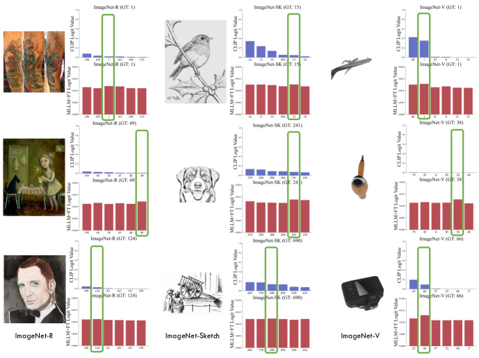
Figure 14: Images with the prediction logits before and after fine-tuning. Examples are randomly choosen from ImageNet-R, ImageNet-Sketch, and ImageNet-V. The green boxes highlight the ground truth class logits.

D.2 Analysis on Various DICL Designs

To justify why using just one positive-negative exemplar pair can effectively conduct vision tasks, here we provide an analysis of using three different DICL designs. Specifically, we consider using two positive exemplars, two negative exemplars, and two incorrect exemplars as baseline DICL designs and compare them to the original MVT results in the main paper. For example, the three types of instructions are shown as:

Two positive exemplars:

Two negative exemplars:

Two incorrect exemplars:

Table 13: Performance of using different DICL prompt designs. We also compare them with the original MVT using ViT-L and fine-tuning performance using the MMICL backbone.

MLLM	Method	ID					OOD
		IN-Val	IN-V2	Cifar10	Cifar100	MNIST	IN-A	IN-R	IN-SK	IN-V	iWildCam
None	CLIP [54]	75.8	70.2	95.6	78.2	76.4	69.3	86.6	59.4	51.8	13.4
MMICL  [75]	Two incorrect	73.2	68.3	93.2	77.6	54.6	68.7	86.8	58.2	58.3	22.3
	Two positive	74.5	69.5	94.1	77.9	56.2	69.0	87.4	57.5	60.9	23.7
	Two negative	75.0	69.0	96.6	78.1	55.7	69.3	87.8	58.1	61.2	24.3
	MVT	75.2	70.8	97.9	78.9	53.0	71.2	88.1	59.0	62.1	25.0
	+FT	76.9	70.5	96.7	82.0	79.2	75.1	89.5	61.4	68.8	-

The results are shown in Table 13. We find that all three designs are inferior to our method MVT, thus we know that using one positive and negative exemplar pair is the most effective instruction strategy. Moreover, we find that using Two negative exemplars is slightly better than the other two, which manifests that negative exemplars are quite important in deciding the effectiveness of MVT, further justifying that using a noise transition matrix to find the most probable negative classes is essential to our method. Furthermore, we also find that using two incorrect exemplars achieves the worst performance, even inferior to CLIP ViT-L. This could be because that feed incorrect instructions could indeed mislead the learning performance, thus showing degradation.

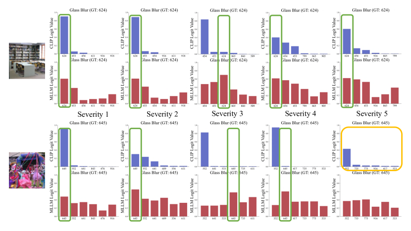
Figure 15: Robustness analysis using ImageNet-C with Glass Blur corruption. The green boxes highlight the logits of ground truth classes, and the orange boxes denote there are no ground truth predictions in the CLIP top-$6$ predictions.

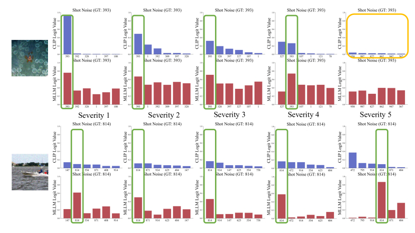
Figure 16: Robustness analysis using ImageNet-C with Glass Blur corruption. The green boxes highlight the logits of ground truth classes, and the orange boxes denote there are no ground truth predictions in the CLIP top-$6$ predictions.

D.3 Analysis on OOD Robustness

To further investigate the performance on facing OOD data with varied strengths, here we use ImageNet-C to show how increasing the corruption severity could affect the prediction of the vision model and MLLM (MMICL). For illustration, we randomly choose four examples from ImageNet-C and plot their top-$6$ prediction logits from the vision model. Moreover, for clear comparison, we also choose the top-$6$ prediction classes as our therapy candidates (which is different from the settings of MVT) to show the MLLM prediction results. As shown in Figures 15 and 16, we can see that as the severity increases, the prediction of CLIP logit values is highly unstable. When the severity is large, the final top-$1$ prediction could be incorrect. However, the prediction of MLLM remains consistent through all severities. Even when CLIP prediction is incorrect, MLLM can still correctly find the ground truth classes. Only when there is no ground truth in top-$6$ predictions, MLLM can be uncertain about the final prediction. Therefore, the robustness of MLLM against corruption could justify that our MVT is quite effective on OOD tasks compared to vision models.

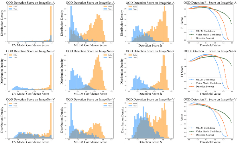
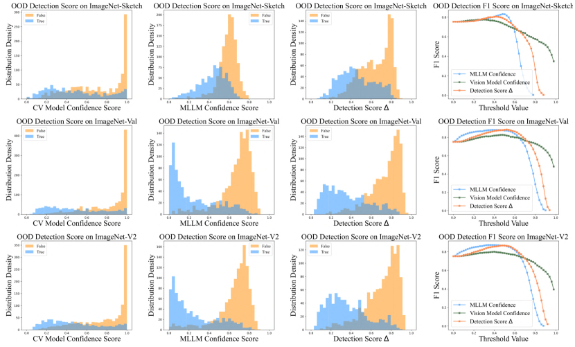
Figure 17: OOD detection performance on ImageNet-A, ImageNet-R, ImageNet-V, ImageNet-Sketch, ImageNet-Val, and ImageNet-V2 datasets using ViT-L. The first three columns: Density distribution of different OOD detection scores; The last column: F1 score values by varying the OOD detection threshold $\delta$.

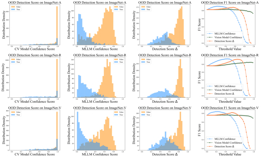
Figure 18: First three rows: OOD detection performance on MNIST, CIFAR10, and CIFAR100 datasets using ViT-L. Last three rows: OOD detection performance on ImageNet-A, ImageNet-R, and ImageNet-V datasets using ViT-g. The first three columns: Density distribution of different OOD detection scores; The last column: F1 score values by varying the OOD detection threshold $\delta$.

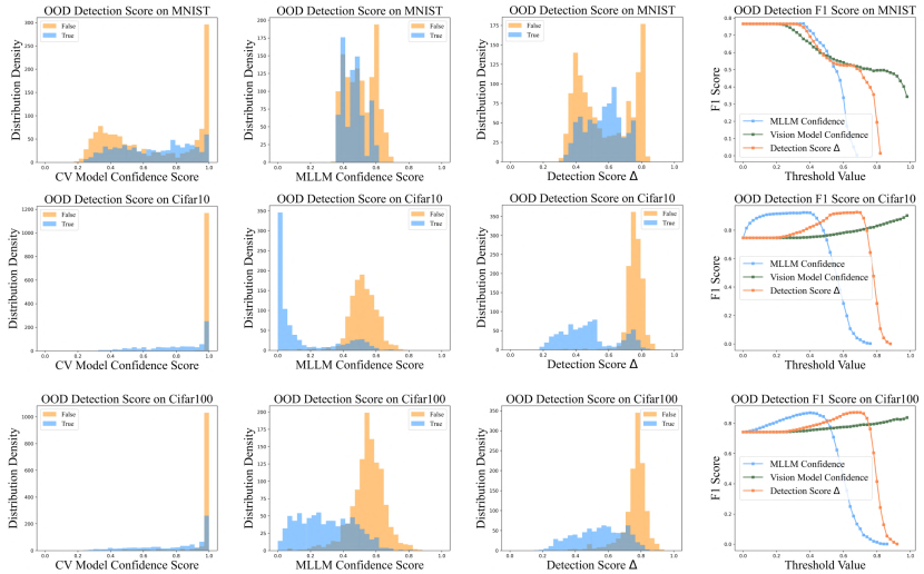
Figure 19: OOD detection performance on ImageNet-Sketch, ImageNet-Val, ImageNet-V2, MNIST, CIFAR10, and CIFAR100 datasets using ViT-g. The first three columns: Density distribution of different OOD detection scores; The last column: F1 score values by varying the OOD detection threshold $\delta$.

D.4 Analysis on OOD Detection

As an extension of the main paper, here we further provide more results on OOD detection. We consider ImageNet-A, ImageNet-R, ImageNet-V, ImageNet-Sketch, ImageNet-Val, ImageNet-V2, MNIST, Cifar10, and Cifar100 datasets using both ViT-L and ViT-g models. The results are shown in Figures 17, 18, 19. We can observe similar phenomenons as in the main paper: MLLM can effectively identify open-class data and vision models can identify close-class data. By combining the prediction confidence of MLLM and vision models, our detection score $\Delta$ can be successfully leveraged to conduct OOD detection, and the F1 score of $\Delta$ can achieve the largest value with a reasonable detection threshold $\delta$. Still, some datasets are relatively challenging compared to other datasets: ImageNet-Sketch and MNIST. This could be due to that the classification performance on these two datasets is not outstanding, about $50\%$ to $68\%$ for both vision models and MLLMs. Moreover, the patterns of such two datasets are quite simple: both of them are handwritten lines without complex natural features, which could further hinder the extraction of useful knowledge, thus leading to sub-optimal detection performance. Overall, the OOD detection performance of MVT is effective on most datasets and the capability of recognizing unknown examples could provide insight to the OOD detection field. We plan to further investigate its potential in future works.

Appendix E Limitation and Broader Impact

In this paper, we proposed an effective framework that aims to enhance the visual robustness of vision models by exploiting the knowledge of MLLMs instead of requiring additional human annotations. Based on our proposed DICL strategy, the paradigm of MLLMs can be perfectly aligned to vision tasks and achieve encouraging results. However, we found that the performance of our MVT is highly related to the ICL capability of MLLMs. Moreover, since there are only two existing MLLMs that possess multimodal ICL power, the potential of our MVT framework could be further improved when sophisticated MLLMs with multimodal ICL abilities are developed in the future. Additionally, we only considered class-dependent noise transition, other challenging scenarios such as instance-dependent noise transition could be further studied in the future. We hope our work could bring insight into the multimodal learning field through our framework to achieve alignment between MLLMs and vision learning tasks. Based on our work, we believe many traditional fields that are related to visual recognition such as weakly-supervised learning, OOD detection, and fine-grained image classification could be further advanced by effectively leveraging the knowledge of MLLMs.

References

- Alayrac et al. [2022] Jean-Baptiste Alayrac, Jeff Donahue, Pauline Luc, Antoine Miech, Iain Barr, Yana Hasson, Karel Lenc, Arthur Mensch, Katherine Millican, Malcolm Reynolds, et al. Flamingo: a visual language model for few-shot learning. In NeurIPS, volume 35, pages 23716–23736, 2022.
- Awadalla et al. [2023] Anas Awadalla, Irena Gao, Josh Gardner, Jack Hessel, Yusuf Hanafy, Wanrong Zhu, Kalyani Marathe, Yonatan Bitton, Samir Gadre, Shiori Sagawa, et al. Openflamingo: An open-source framework for training large autoregressive vision-language models. arXiv preprint arXiv:2308.01390, 2023.
- Brown et al. [2020] Tom Brown, Benjamin Mann, Nick Ryder, Melanie Subbiah, Jared D Kaplan, Prafulla Dhariwal, Arvind Neelakantan, Pranav Shyam, Girish Sastry, Amanda Askell, et al. Language models are few-shot learners. Advances in neural information processing systems, 33:1877–1901, 2020.
- Chang et al. [2020] Shiyu Chang, Yang Zhang, Mo Yu, and Tommi Jaakkola. Invariant rationalization. In International Conference on Machine Learning, pages 1448–1458. PMLR, 2020.
- Chen et al. [2023] Yixin Chen, Shuai Zhang, Boran Han, and Jiaya Jia. Lightweight in-context tuning for multimodal unified models. arXiv preprint arXiv:2310.05109, 2023.
- Chiang et al. [2023] Wei-Lin Chiang, Zhuohan Li, Zi Lin, Ying Sheng, Zhanghao Wu, Hao Zhang, Lianmin Zheng, Siyuan Zhuang, Yonghao Zhuang, Joseph E. Gonzalez, Ion Stoica, and Eric P. Xing. Vicuna: An open-source chatbot impressing gpt-4 with 90%* chatgpt quality, March 2023. URL https://lmsys.org/blog/2023-03-30-vicuna/.
- Chung et al. [2022] Hyung Won Chung, Le Hou, Shayne Longpre, Barret Zoph, Yi Tay, William Fedus, Yunxuan Li, Xuezhi Wang, Mostafa Dehghani, Siddhartha Brahma, et al. Scaling instruction-finetuned language models. arXiv preprint arXiv:2210.11416, 2022.
- Dai et al. [2023] Wenliang Dai, Junnan Li, Dongxu Li, Anthony Meng Huat Tiong, Junqi Zhao, Weisheng Wang, Boyang Li, Pascale Fung, and Steven Hoi. Instructblip: Towards general-purpose vision-language models with instruction tuning. arXiv preprint arXiv:2305.06500, 2023.
- Deng et al. [2009] Jia Deng, Wei Dong, Richard Socher, Li-Jia Li, Kai Li, and Li Fei-Fei. Imagenet: A large-scale hierarchical image database. In 2009 IEEE conference on computer vision and pattern recognition, pages 248–255. Ieee, 2009.
- DeVries and Taylor [2017] Terrance DeVries and Graham W Taylor. Improved regularization of convolutional neural networks with cutout. arXiv preprint arXiv:1708.04552, 2017.
- Dong et al. [2022] Yinpeng Dong, Shouwei Ruan, Hang Su, Caixin Kang, Xingxing Wei, and Jun Zhu. Viewfool: Evaluating the robustness of visual recognition to adversarial viewpoints. Advances in Neural Information Processing Systems, 35:36789–36803, 2022.
- Dong et al. [2023] Yinpeng Dong, Caixin Kang, Jinlai Zhang, Zijian Zhu, Yikai Wang, Xiao Yang, Hang Su, Xingxing Wei, and Jun Zhu. Benchmarking robustness of 3d object detection to common corruptions in autonomous driving. arXiv preprint arXiv:2303.11040, 2023.
- Dosovitskiy et al. [2020] Alexey Dosovitskiy, Lucas Beyer, Alexander Kolesnikov, Dirk Weissenborn, Xiaohua Zhai, Thomas Unterthiner, Mostafa Dehghani, Matthias Minderer, Georg Heigold, Sylvain Gelly, et al. An image is worth 16x16 words: Transformers for image recognition at scale. arXiv preprint arXiv:2010.11929, 2020.
- Fang et al. [2022] Yuxin Fang, Wen Wang, Binhui Xie, Quan Sun, Ledell Wu, Xinggang Wang, Tiejun Huang, Xinlong Wang, and Yue Cao. Eva: Exploring the limits of masked visual representation learning at scale. arXiv preprint arXiv:2211.07636, 2022.
- Floridi and Chiriatti [2020] Luciano Floridi and Massimo Chiriatti. Gpt-3: Its nature, scope, limits, and consequences. Minds and Machines, 30:681–694, 2020.
- Frénay and Verleysen [2013] Benoît Frénay and Michel Verleysen. Classification in the presence of label noise: a survey. IEEE transactions on neural networks and learning systems, 25(5):845–869, 2013.
- Girdhar et al. [2023] Rohit Girdhar, Alaaeldin El-Nouby, Zhuang Liu, Mannat Singh, Kalyan Vasudev Alwala, Armand Joulin, and Ishan Misra. Imagebind: One embedding space to bind them all. In CVPR, 2023.
- Gong et al. [2023] Tao Gong, Chengqi Lyu, Shilong Zhang, Yudong Wang, Miao Zheng, Qian Zhao, Kuikun Liu, Wenwei Zhang, Ping Luo, and Kai Chen. Multimodal-gpt: A vision and language model for dialogue with humans. arXiv preprint arXiv:2305.04790, 2023.
- Goyal et al. [2023] Sachin Goyal, Ananya Kumar, Sankalp Garg, Zico Kolter, and Aditi Raghunathan. Finetune like you pretrain: Improved finetuning of zero-shot vision models. In CVPR, pages 19338–19347, 2023.
- Gulrajani and Lopez-Paz [2020] Ishaan Gulrajani and David Lopez-Paz. In search of lost domain generalization. arXiv preprint arXiv:2007.01434, 2020.
- Gulrajani and Lopez-Paz [2021] Ishaan Gulrajani and David Lopez-Paz. In search of lost domain generalization. In ICLR, 2021.
- Han et al. [2018] Bo Han, Quanming Yao, Xingrui Yu, Gang Niu, Miao Xu, Weihua Hu, Ivor Tsang, and Masashi Sugiyama. Co-teaching: Robust training of deep neural networks with extremely noisy labels. In NeurIPS, volume 31, 2018.
- Hendrycks and Dietterich [2019] Dan Hendrycks and Thomas Dietterich. Benchmarking neural network robustness to common corruptions and perturbations. In ICLR, 2019.
- Hendrycks and Gimpel [2016] Dan Hendrycks and Kevin Gimpel. A baseline for detecting misclassified and out-of-distribution examples in neural networks. In ICLR, 2016.
- Hendrycks et al. [2018] Dan Hendrycks, Mantas Mazeika, and Thomas Dietterich. Deep anomaly detection with outlier exposure. arXiv preprint arXiv:1812.04606, 2018.
- Hendrycks et al. [2021a] Dan Hendrycks, Steven Basart, Norman Mu, Saurav Kadavath, Frank Wang, Evan Dorundo, Rahul Desai, Tyler Zhu, Samyak Parajuli, Mike Guo, et al. The many faces of robustness: A critical analysis of out-of-distribution generalization. In Proceedings of the IEEE/CVF International Conference on Computer Vision, pages 8340–8349, 2021a.
- Hendrycks et al. [2021b] Dan Hendrycks, Kevin Zhao, Steven Basart, Jacob Steinhardt, and Dawn Song. Natural adversarial examples. In CVPR, pages 15262–15271, 2021b.
- Hu et al. [2021] Edward J Hu, Yelong Shen, Phillip Wallis, Zeyuan Allen-Zhu, Yuanzhi Li, Shean Wang, Lu Wang, and Weizhu Chen. Lora: Low-rank adaptation of large language models. arXiv preprint arXiv:2106.09685, 2021.
- Huang et al. [2023a] Shaohan Huang, Li Dong, Wenhui Wang, Yaru Hao, Saksham Singhal, Shuming Ma, Tengchao Lv, Lei Cui, Owais Khan Mohammed, Qiang Liu, et al. Language is not all you need: Aligning perception with language models. arXiv preprint arXiv:2302.14045, 2023a.
- Huang et al. [2023b] Zhuo Huang, Muyang Li, Li Shen, Jun Yu, Chen Gong, Bo Han, and Tongliang Liu. Winning prize comes from losing tickets: Improve invariant learning by exploring variant parameters for out-of-distribution generalization. arXiv preprint arXiv:2310.16391, 2023b.
- Huang et al. [2023c] Zhuo Huang, Xiaobo Xia, Li Shen, Bo Han, Mingming Gong, Chen Gong, and Tongliang Liu. Harnessing out-of-distribution examples via augmenting content and style. In ICLR, 2023c.
- Huang et al. [2023d] Zhuo Huang, Miaoxi Zhu, Xiaobo Xia, Li Shen, Jun Yu, Chen Gong, Bo Han, Bo Du, and Tongliang Liu. Robust generalization against photon-limited corruptions via worst-case sharpness minimization. In Proceedings of the IEEE/CVF Conference on Computer Vision and Pattern Recognition, pages 16175–16185, 2023d.
- Jia et al. [2021] Chao Jia, Yinfei Yang, Ye Xia, Yi-Ting Chen, Zarana Parekh, Hieu Pham, Quoc Le, Yun-Hsuan Sung, Zhen Li, and Tom Duerig. Scaling up visual and vision-language representation learning with noisy text supervision. In ICML, pages 4904–4916. PMLR, 2021.
- Koh et al. [2021a] Pang Wei Koh, Shiori Sagawa, Henrik Marklund, Sang Michael Xie, Marvin Zhang, Akshay Balsubramani, Weihua Hu, Michihiro Yasunaga, Richard Lanas Phillips, Irena Gao, Tony Lee, Etienne David, Ian Stavness, Wei Guo, Berton A. Earnshaw, Imran S. Haque, Sara Beery, Jure Leskovec, Anshul Kundaje, Emma Pierson, Sergey Levine, Chelsea Finn, and Percy Liang. WILDS: A benchmark of in-the-wild distribution shifts. In International Conference on Machine Learning (ICML), 2021a.
- Koh et al. [2021b] Pang Wei Koh, Shiori Sagawa, Henrik Marklund, Sang Michael Xie, Marvin Zhang, Akshay Balsubramani, Weihua Hu, Michihiro Yasunaga, Richard Lanas Phillips, Irena Gao, et al. Wilds: A benchmark of in-the-wild distribution shifts. In ICML, pages 5637–5664. PMLR, 2021b.
- Krizhevsky et al. [2009] Alex Krizhevsky, Geoffrey Hinton, et al. Learning multiple layers of features from tiny images. 2009.
- LeCun et al. [1998] Yann LeCun, Léon Bottou, Yoshua Bengio, and Patrick Haffner. Gradient-based learning applied to document recognition. Proceedings of the IEEE, 86(11):2278–2324, 1998.
- Li et al. [2023a] Bo Li, Yuanhan Zhang, Liangyu Chen, Jinghao Wang, Fanyi Pu, Jingkang Yang, Chunyuan Li, and Ziwei Liu. Mimic-it: Multi-modal in-context instruction tuning. 2023a.
- Li et al. [2023b] Bo Li, Yuanhan Zhang, Liangyu Chen, Jinghao Wang, Jingkang Yang, and Ziwei Liu. Otter: A multi-modal model with in-context instruction tuning. arXiv preprint arXiv:2305.03726, 2023b.
- Li et al. [2022] Junnan Li, Dongxu Li, Caiming Xiong, and Steven Hoi. Blip: Bootstrapping language-image pre-training for unified vision-language understanding and generation. In International Conference on Machine Learning, pages 12888–12900. PMLR, 2022.
- Li et al. [2023c] Junnan Li, Dongxu Li, Silvio Savarese, and Steven Hoi. Blip-2: Bootstrapping language-image pre-training with frozen image encoders and large language models. arXiv preprint arXiv:2301.12597, 2023c.
- Li et al. [2021] Yangguang Li, Feng Liang, Lichen Zhao, Yufeng Cui, Wanli Ouyang, Jing Shao, Fengwei Yu, and Junjie Yan. Supervision exists everywhere: A data efficient contrastive language-image pre-training paradigm. arXiv preprint arXiv:2110.05208, 2021.
- Li et al. [2023d] Yanghao Li, Haoqi Fan, Ronghang Hu, Christoph Feichtenhofer, and Kaiming He. Scaling language-image pre-training via masking. In CVPR, pages 23390–23400, June 2023d.
- Liu et al. [2023] Haotian Liu, Chunyuan Li, Qingyang Wu, and Yong Jae Lee. Visual instruction tuning. In NeurIPS, 2023.
- Liu and Tao [2015] Tongliang Liu and Dacheng Tao. Classification with noisy labels by importance reweighting. IEEE Transactions on pattern analysis and machine intelligence, 38(3):447–461, 2015.
- Liu et al. [2020] Weitang Liu, Xiaoyun Wang, John Owens, and Yixuan Li. Energy-based out-of-distribution detection. In NeurIPS, volume 33, pages 21464–21475, 2020.
- Liu et al. [2021] Ze Liu, Yutong Lin, Yue Cao, Han Hu, Yixuan Wei, Zheng Zhang, Stephen Lin, and Baining Guo. Swin transformer: Hierarchical vision transformer using shifted windows. In ICCV, pages 10012–10022, 2021.
- Liu et al. [2015] Ziwei Liu, Ping Luo, Xiaogang Wang, and Xiaoou Tang. Deep learning face attributes in the wild. In Proceedings of International Conference on Computer Vision (ICCV), December 2015.
- Lynch et al. [2023] Aengus Lynch, Gbètondji JS Dovonon, Jean Kaddour, and Ricardo Silva. Spawrious: A benchmark for fine control of spurious correlation biases. arXiv preprint arXiv:2303.05470, 2023.
- Mahajan et al. [2021] Divyat Mahajan, Shruti Tople, and Amit Sharma. Domain generalization using causal matching. In International Conference on Machine Learning, pages 7313–7324. PMLR, 2021.
- Mu et al. [2022] Norman Mu, Alexander Kirillov, David Wagner, and Saining Xie. Slip: Self-supervision meets language-image pre-training. In ECCV, pages 529–544. Springer, 2022.
- Natarajan et al. [2013] Nagarajan Natarajan, Inderjit S Dhillon, Pradeep K Ravikumar, and Ambuj Tewari. Learning with noisy labels. In NeurIPS, volume 26, 2013.
- OpenAI [2023] OpenAI. Gpt-4 technical report, 2023.
- Radford et al. [2021] Alec Radford, Jong Wook Kim, Chris Hallacy, Aditya Ramesh, Gabriel Goh, Sandhini Agarwal, Girish Sastry, Amanda Askell, Pamela Mishkin, Jack Clark, et al. Learning transferable visual models from natural language supervision. In ICML, pages 8748–8763. PMLR, 2021.
- Recht et al. [2019] Benjamin Recht, Rebecca Roelofs, Ludwig Schmidt, and Vaishaal Shankar. Do imagenet classifiers generalize to imagenet? In International conference on machine learning, pages 5389–5400. PMLR, 2019.
- Scao et al. [2022] Teven Le Scao, Angela Fan, Christopher Akiki, Ellie Pavlick, Suzana Ilić, Daniel Hesslow, Roman Castagné, Alexandra Sasha Luccioni, François Yvon, Matthias Gallé, et al. Bloom: A 176b-parameter open-access multilingual language model. arXiv preprint arXiv:2211.05100, 2022.
- Shu et al. [2023] Yang Shu, Xingzhuo Guo, Jialong Wu, Ximei Wang, Jianmin Wang, and Mingsheng Long. Clipood: Generalizing clip to out-of-distributions. In ICML. PMLR, 2023.
- Su et al. [2023] Yixuan Su, Tian Lan, Huayang Li, Jialu Xu, Yan Wang, and Deng Cai. Pandagpt: One model to instruction-follow them all. arXiv preprint arXiv:2305.16355, 2023.
- Touvron et al. [2023a] Hugo Touvron, Thibaut Lavril, Gautier Izacard, Xavier Martinet, Marie-Anne Lachaux, Timothée Lacroix, Baptiste Rozière, Naman Goyal, Eric Hambro, Faisal Azhar, et al. Llama: Open and efficient foundation language models. arXiv preprint arXiv:2302.13971, 2023a.
- Touvron et al. [2023b] Hugo Touvron, Louis Martin, Kevin Stone, Peter Albert, Amjad Almahairi, Yasmine Babaei, Nikolay Bashlykov, Soumya Batra, Prajjwal Bhargava, Shruti Bhosale, et al. Llama 2: Open foundation and fine-tuned chat models. arXiv preprint arXiv:2307.09288, 2023b.
- Wang et al. [2019] Haohan Wang, Songwei Ge, Zachary Lipton, and Eric P Xing. Learning robust global representations by penalizing local predictive power. In NeurIPS, volume 32, 2019.
- Wang et al. [2022] Jianfeng Wang, Zhengyuan Yang, Xiaowei Hu, Linjie Li, Kevin Lin, Zhe Gan, Zicheng Liu, Ce Liu, and Lijuan Wang. Git: A generative image-to-text transformer for vision and language. arXiv preprint arXiv:2205.14100, 2022.
- Wang et al. [2021] Wenhai Wang, Enze Xie, Xiang Li, Deng-Ping Fan, Kaitao Song, Ding Liang, Tong Lu, Ping Luo, and Ling Shao. Pyramid vision transformer: A versatile backbone for dense prediction without convolutions. In ICCV, pages 568–578, 2021.
- Wortsman et al. [2022] Mitchell Wortsman, Gabriel Ilharco, Jong Wook Kim, Mike Li, Simon Kornblith, Rebecca Roelofs, Raphael Gontijo Lopes, Hannaneh Hajishirzi, Ali Farhadi, Hongseok Namkoong, et al. Robust fine-tuning of zero-shot models. In CVPR, pages 7959–7971, 2022.
- Xia et al. [2019] Xiaobo Xia, Tongliang Liu, Nannan Wang, Bo Han, Chen Gong, Gang Niu, and Masashi Sugiyama. Are anchor points really indispensable in label-noise learning? In NeurIPS, volume 32, 2019.
- Xia et al. [2020] Xiaobo Xia, Tongliang Liu, Bo Han, Nannan Wang, Mingming Gong, Haifeng Liu, Gang Niu, Dacheng Tao, and Masashi Sugiyama. Part-dependent label noise: Towards instance-dependent label noise. In NeurIPS, volume 33, pages 7597–7610, 2020.
- Xie et al. [2021] Sang Michael Xie, Aditi Raghunathan, Percy Liang, and Tengyu Ma. An explanation of in-context learning as implicit bayesian inference. arXiv preprint arXiv:2111.02080, 2021.
- Yasunaga et al. [2023] Michihiro Yasunaga, Armen Aghajanyan, Weijia Shi, Richard James, Jure Leskovec, Percy Liang, Mike Lewis, Luke Zettlemoyer, and Wen-tau Yih. Retrieval-augmented multimodal language modeling. In ICML, 2023.
- Ye et al. [2023] Qinghao Ye, Haiyang Xu, Guohai Xu, Jiabo Ye, Ming Yan, Yiyang Zhou, Junyang Wang, Anwen Hu, Pengcheng Shi, Yaya Shi, et al. mplug-owl: Modularization empowers large language models with multimodality. arXiv preprint arXiv:2304.14178, 2023.
- Yun et al. [2019] Sangdoo Yun, Dongyoon Han, Seong Joon Oh, Sanghyuk Chun, Junsuk Choe, and Youngjoon Yoo. Cutmix: Regularization strategy to train strong classifiers with localizable features. In Proceedings of the IEEE/CVF International Conference on Computer Vision, pages 6023–6032, 2019.
- Zhai et al. [2022] Xiaohua Zhai, Alexander Kolesnikov, Neil Houlsby, and Lucas Beyer. Scaling vision transformers. In Proceedings of the IEEE/CVF Conference on Computer Vision and Pattern Recognition, pages 12104–12113, 2022.
- Zhai et al. [2023] Yuexiang Zhai, Shengbang Tong, Xiao Li, Mu Cai, Qing Qu, Yong Jae Lee, and Yi Ma. Investigating the catastrophic forgetting in multimodal large language models. arXiv preprint arXiv:2309.10313, 2023.
- Zhang et al. [2017] Hongyi Zhang, Moustapha Cisse, Yann N Dauphin, and David Lopez-Paz. mixup: Beyond empirical risk minimization. arXiv preprint arXiv:1710.09412, 2017.
- Zhang et al. [2022] Susan Zhang, Stephen Roller, Naman Goyal, Mikel Artetxe, Moya Chen, Shuohui Chen, Christopher Dewan, Mona Diab, Xian Li, Xi Victoria Lin, et al. Opt: Open pre-trained transformer language models. arXiv preprint arXiv:2205.01068, 2022.
- Zhao et al. [2023] Haozhe Zhao, Zefan Cai, Shuzheng Si, Xiaojian Ma, Kaikai An, Liang Chen, Zixuan Liu, Sheng Wang, Wenjuan Han, and Baobao Chang. Mmicl: Empowering vision-language model with multi-modal in-context learning. arXiv preprint arXiv:2309.07915, 2023.
- Zheng et al. [2023] Lianmin Zheng, Wei-Lin Chiang, Ying Sheng, Siyuan Zhuang, Zhanghao Wu, Yonghao Zhuang, Zi Lin, Zhuohan Li, Dacheng Li, Eric. P Xing, Hao Zhang, Joseph E. Gonzalez, and Ion Stoica. Judging llm-as-a-judge with mt-bench and chatbot arena, 2023.
- Zhu et al. [2023a] Deyao Zhu, Jun Chen, Xiaoqian Shen, Xiang Li, and Mohamed Elhoseiny. Minigpt-4: Enhancing vision-language understanding with advanced large language models. arXiv preprint arXiv:2304.10592, 2023a.
- Zhu et al. [2023b] Zijian Zhu, Yichi Zhang, Hai Chen, Yinpeng Dong, Shu Zhao, Wenbo Ding, Jiachen Zhong, and Shibao Zheng. Understanding the robustness of 3d object detection with bird’s-eye-view representations in autonomous driving. In Proceedings of the IEEE/CVF Conference on Computer Vision and Pattern Recognition, pages 21600–21610, 2023b.