The general linear hypothesis testing problem for multivariate functional data with applications

Abstract

As technology continues to advance at a rapid pace, the prevalence of multivariate functional data (MFD) has expanded across diverse disciplines, spanning biology, climatology, finance, and numerous other fields of study. Although MFD are encountered in various fields, the development of methods for hypotheses on mean functions, especially the general linear hypothesis testing (GLHT) problem for such data has been limited. In this study, we propose and study a new global test for the GLHT problem for MFD, which includes the one-way FMANOVA, post hoc, and contrast analysis as special cases. The asymptotic null distribution of the test statistic is shown to be a chi-squared-type mixture dependent of eigenvalues of the heteroscedastic covariance functions. The distribution of the chi-squared-type mixture can be well approximated by a three-cumulant matched chi-squared-approximation with its approximation parameters estimated from the data. By incorporating an adjustment coefficient, the proposed test performs effectively irrespective of the correlation structure in the functional data, even when dealing with a relatively small sample size. Additionally, the proposed test is shown to be root-$n$ consistent, that is, it has a nontrivial power against a local alternative. Simulation studies and a real data example demonstrate finite-sample performance and broad applicability of the proposed test.

Keywords: Heteroscedastic one-way MANOVA, contrast analysis, chi-squared-type mixture, three-cumulant matched chi-squared-approximation, nonparametric bootstrapping.

1 Introduction

With the rapid evolution of technology, data are increasingly being acquired and represented as trajectories or images in various scientific domains. This trend can be observed in disciplines such as meteorology, biology, medicine, and engineering, among others. Consequently, functional data analysis (FDA) has emerged as a prominent field of study with significant applications across numerous real-world domains. It is a branch of statistics concerned with the analysis of infinite-dimensional variables and can be treated as a generalization of the standard multivariate data analysis. The work of this paper is partially motivated by a financial data set provided by the Credit Research Initiative of National University of Singapore (NUS-CRI). The Probability of Default (PD) is a metric used to quantify the likelihood of an obligor being unable to honor its financial obligations and is the core credit product of the NUS-CRI corporate default prediction system built on the forward intensity model of Duan et al. (2012). This financial data set contains the mean PD values aggregated by the economy of domicile and sector of each firm from 2012 to 2021. As a result, each economy can be represented by multiple curves, with each curve representing the aggregate PD of a specific sector, illustrating an example of multivariate functional observations. It is of interest to compare the mean aggregated PD curves corresponding to four important factors, namely, energy, financial, real estate, and industrial in the various regions, including Asia Pacific (Developed), Asia Pacific (Emerging), Eurozone, and Non-Eurozone are all the same. This leads to a $k$-sample problem for multivariate functional data (MFD) which is a special case of the general linear hypothesis testing (GLHT) problem for MFD.

Mathematically, a general $k$-sample problem, also known as one-way multivariate analysis of variance for functional data (FMANOVA) can be described as follows. Let $\operatorname{SP}_{p}({\bf\bm{\mathit{\eta}}},{\bf\bm{\mathit{\Gamma}}})$ denote a $p$-dimensional stochastic process with vector of mean functions ${\bf\bm{\mathit{\eta}}}(t),t\in\mathcal{T}$, and matrix of covariance functions ${\bf\bm{\mathit{\Gamma}}}(s,t),(s,t)\in\mathcal{T}^{2}$, where $\mathcal{T}$ is the time period of interest, often a finite interval $[a,b]$ say with $-\infty<a<b<\infty$. For simplicity of notation, throughout this paper, we use $\mathcal{T}^{2}$ and $\mathcal{T}^{3}$ to denote the direct products of $\mathcal{T}\otimes\mathcal{T}$ and $\mathcal{T}\otimes\mathcal{T}\otimes\mathcal{T}$, respectively. Suppose we have $k$ independent functional samples

$${\bf\bm{\mathit{y}}}_{\alpha 1}(t),\ldots,{\bf\bm{\mathit{y}}}_{\alpha n_{\alpha}}(t)\stackrel{{\scriptstyle\text{i.i.d.}}}{{\sim}}\operatorname{SP}_{p}({\bf\bm{\mathit{\eta}}}_{\alpha},{\bf\bm{\mathit{\Gamma}}}_{\alpha}),\;\alpha=1,\ldots,k,$$ (1)

where ${\bf\bm{\mathit{\eta}}}_{\alpha}(t),\alpha=1,\ldots,k$ are the unknown vectors of group mean function of the $k$ samples and ${\bf\bm{\mathit{\Gamma}}}_{\alpha}(s,t)=\operatorname{Cov}[{\bf\bm{\mathit{y}}}_{\alpha 1}(s),{\bf\bm{\mathit{y}}}_{\alpha 1}(t)],\alpha=1,\ldots,k$ are the unknown matrices of covariance functions. Note that we assume the functional observations from the same group are independent and identically distributed (i.i.d.) and the functional observations from different groups are also independent. One may wish to test whether the $k$ mean functions are equal:

$$H_{0}:{\bf\bm{\mathit{\eta}}}_{1}(t)=\cdots={\bf\bm{\mathit{\eta}}}_{k}(t),\;\forall t\in\mathcal{T}$$ (2)

against the usual alternative that at least two of the vectors of mean function are not the same. For the above problem, several interesting tests have been proposed by a number of authors. First of all, when $p=1$, meaning that the FMANVOA problem in (1) is simplified to one-way ANOVA problem for functional data (FANOVA). Numerous tests have been put forth for the FANOVA problem and have been employed in various practical scenarios, such as ischemic heart screening and detecting changes in air pollution during the COVID-19 pandemic, including Cuevas et al. (2004); Cuesta-Albertos and Febrero-Bande (2010); Zhang (2013); Zhang and Liang (2014); Zhang et al. (2019); Acal et al. (2022). In particular, (Zhang, 2013, Chapter 6) proposed three methods for the GLHT problem for univariate functional data, namely, the pointwise $F$, $L^{2}$-norm-based, and $F$-type tests. Smaga and Zhang (2019) studied the theoretical properties of the above $L^{2}$-norm-based test and $F$-type test, and proposed two new testing procedures by globalizing pointwise $F$-test and the $F_{\max}$-test. When $p>1$, Qiu et al. (2021) first proposed two global tests for the two-sample problem for MFD. Górecki and Smaga (2017) defined the “between” and “within” matrices for MFD, and then used them to construct several test statistics, including the Wilks lambda test statistic, the Lawley–Hotelling trace test statistic, the Pillai trace test statistic and Roy’s maximum root test statistic. Zhu et al. (2022) proposed the Lawley–Hotelling trace test for the FMANOVA problem by assuming that the matrices of covariance functions of the $k$ samples are the same, while Zhu et al. (2023) introduced a global test statistic for the heteroscedastic FMANOVA problem. Although some work has been done for the one-way FMANOVA problem, the post hoc or contrast analysis is not satisfactorily developed in the literature. Up to my knowledge, this study may be the first work for the above GLHT problem for MFD.

In this study, given the $k$ independent samples (1), we are interested in testing the following GLHT problem for MFD:

$$H_{0}:{\bf\bm{\mathit{G}}}{\bf\bm{\mathit{M}}}(t)={\bf\bm{\mathit{0}}},\;t\in\mathcal{T}\mbox{ vs. }H_{1}:{\bf\bm{\mathit{G}}}{\bf\bm{\mathit{M}}}(t)\neq{\bf\bm{\mathit{0}}},\;\mbox{for some }t\in\mathcal{T},$$ (3)

where ${\bf\bm{\mathit{M}}}(t)=[\bm{\eta}_{1}(t),\ldots,\bm{\eta}_{k}(t)]^{\top}$ is a $k\times p$ matrix at time point $t$ whose rows are the $k$ mean functions, and ${\bf\bm{\mathit{G}}}:q\times k$ is a known coefficient matrix with $rank({\bf\bm{\mathit{G}}})=q<k$. The GLHT problem (3) is very general. Many particular hypothesis testing problems can be represented by a general testing framework described above. For example, when we set ${\bf\bm{\mathit{G}}}$ to be either ${\bf\bm{\mathit{G}}}_{1}=[{\bf\bm{\mathit{I}}}_{k-1},-\bm{1}_{k-1}]$ or ${\bf\bm{\mathit{G}}}_{2}=[-\bm{1}_{k-1},{\bf\bm{\mathit{I}}}_{k-1}]$, a contrast matrix whose rows sum up to $0$, where ${\bf\bm{\mathit{I}}}_{k}$ and $\bm{1}_{k}$ denote the identity matrix of size $k\times k$ and a $k$-dimensional vector of ones, respectively, the GLHT problem (3) reduces to an one-way FMANOVA problem (2). When the null hypothesis in (2) is rejected, it is often of interest to further test if ${\bf\bm{\mathit{\eta}}}_{1}(t)=c_{1}{\bf\bm{\mathit{\eta}}}_{3}(t),\;\forall t\in\mathcal{T}$ or if a contrast is zero, e.g., $c_{2}{\bf\bm{\mathit{\eta}}}_{1}(t)-(c_{2}+c_{3}){\bf\bm{\mathit{\eta}}}_{2}(t)+c_{3}{\bf\bm{\mathit{\eta}}}_{3}(t)={\bf\bm{\mathit{0}}}$ where $c_{1},c_{2}$, and $c_{3}$ are some known constants. To write the above two testing problems in the form of (3), we can set ${\bf\bm{\mathit{G}}}=(\bm{e}_{1,k}-c_{1}\bm{e}_{3,k})^{\top}$ and ${\bf\bm{\mathit{G}}}=(c_{2}\bm{e}_{1,k}-(c_{2}+c_{3})\bm{e}_{2,k}+c_{3}\bm{e}_{3,k})^{\top}$, respectively, where and throughout $\bm{e}_{r,l}$ denotes a unit vector of length $l$ with the $r$-th entry being 1 and others 0. It is clear that the contrast matrix ${\bf\bm{\mathit{G}}}$ is not unique. Therefore, it is important to construct a test which is invariant under the following transformation of the coefficient matrix ${\bf\bm{\mathit{G}}}:{\bf\bm{\mathit{G}}}\to{\bf\bm{\mathit{P}}}{\bf\bm{\mathit{G}}}$, where ${\bf\bm{\mathit{P}}}$ is any $q\times q$ non-singular matrix. The GLHT problem (3) can be equivalently re-written as

$$H_{0}:\widetilde{{\bf\bm{\mathit{G}}}}{\bf\bm{\mathit{M}}}(t)={\bf\bm{\mathit{0}}},\;t\in\mathcal{T}\mbox{ vs. }H_{1}:\widetilde{{\bf\bm{\mathit{G}}}}{\bf\bm{\mathit{M}}}(t)\neq{\bf\bm{\mathit{0}}},\;\mbox{for some }t\in\mathcal{T},$$ (4)

where $\widetilde{{\bf\bm{\mathit{G}}}}=({\bf\bm{\mathit{G}}}{\bf\bm{\mathit{D}}}{\bf\bm{\mathit{G}}}^{\top})^{-1/2}{\bf\bm{\mathit{G}}}$ and ${\bf\bm{\mathit{D}}}=\operatorname{diag}(1/n_{1},\ldots,1/n_{k})$.

In this article, we propose a new global test for the GLHT problem (3) which can be employed in a wider range of scenarios or research contexts beyond the specific framework proposed by Qiu et al. (2021), Górecki and Smaga (2017), Zhu et al. (2022) and Zhu et al. (2023). Our main contributions can be described as follows. Firstly, we establish the pointwise variation matrices due to hypothesis for the GLHT problem (3) and due to error, respectively, which serve as the foundation for constructing the pointwise test statistic. By globalizing the pointwise test statistic, we derive the test statistic for our new global test. Secondly, under some regularity conditions and null hypothesis, we show that the asymptotic distribution of the new global test statistic is a chi-squared-type mixture with the mixing coefficients dependent on the matrices of covariance functions. Thirdly, since the asymptotic null distribution of the test statistic is a chi-squared-type mixture, we employ the three-cumulant (3-c) matched chi-squared-approximation of Zhang (2005) to approximate it with the parameters estimated from the data. Then, the proposed new global test can be conducted using the approximate critical value or the approximate $p$-value. Fourthly, we introduce an adjustment coefficient that effectively enhances the performance of our proposed test, even with a relatively small sample size. Fifthly, we also derive asymptotic power of the new global test under some local alternatives and show that it is root-$n$ consistent. Last but not least, simulation results presented in Section 3 show that our new global test has a wider range of applications and outperforms its competitors in terms of size control and power, regardless of whether the functional data are nearly uncorrelated, moderately correlated, or highly correlated.

The rest of this paper is organized as follows. The main results are presented in Section 2. Simulation studies and real data applications are given in Sections 3 and 4, respectively. Technical proofs for the main results are outlined in Appendix.

2 Main Results

2.1 Test Statistic

For each $\alpha=1,\ldots,k$, based on the $\alpha$-th sample in (1) only, the vector of mean functions ${\bf\bm{\mathit{\eta}}}_{\alpha}(t)$ and matrix of covariance functions ${\bf\bm{\mathit{\Gamma}}}_{\alpha}(s,t)$ can be unbiasedly estimated by

$$\begin{array}[]{rcl}\widehat{{\bf\bm{\mathit{\eta}}}}_{\alpha}(t)&=&\bar{{\bf\bm{\mathit{y}}}}_{\alpha}(t)=n_{\alpha}^{-1}\sum_{i=1}^{n_{\alpha}}{\bf\bm{\mathit{y}}}_{\alpha i}(t),\;\mbox{ and }\\ \widehat{{\bf\bm{\mathit{\Gamma}}}}_{\alpha}(s,t)&=&(n_{\alpha}-1)^{-1}\sum_{i=1}^{n_{\alpha}}[{\bf\bm{\mathit{y}}}_{\alpha i}(s)-\bar{{\bf\bm{\mathit{y}}}}_{\alpha}(s)][{\bf\bm{\mathit{y}}}_{\alpha i}(t)-\bar{{\bf\bm{\mathit{y}}}}_{\alpha}(t)]^{\top},\end{array}$$ (5)

which are known as vector of sample mean functions and matrix of sample covariance functions, respectively.

To test (4), we construct the pointwise variation matrix due to hypothesis for the GLHT problem (3) as ${\bf\bm{\mathit{B}}}_{n}(t)=[{\bf\bm{\mathit{G}}}\widehat{{\bf\bm{\mathit{M}}}}(t)]^{\top}({\bf\bm{\mathit{G}}}{\bf\bm{\mathit{D}}}{\bf\bm{\mathit{G}}}^{\top})^{-1}[{\bf\bm{\mathit{G}}}\widehat{{\bf\bm{\mathit{M}}}}(t)]$, where $\widehat{{\bf\bm{\mathit{M}}}}(t)=[\bar{{\bf\bm{\mathit{y}}}}_{1}(t),\ldots,\bar{{\bf\bm{\mathit{y}}}}_{k}(t)]^{\top}$ is the usual unbiased estimator of ${\bf\bm{\mathit{M}}}(t)$. Let ${\bf\bm{\mathit{H}}}={\bf\bm{\mathit{G}}}^{\top}\left({\bf\bm{\mathit{G}}}{\bf\bm{\mathit{D}}}{\bf\bm{\mathit{G}}}^{\top}\right)^{-1}{\bf\bm{\mathit{G}}}$. Then the expectation of ${\bf\bm{\mathit{B}}}_{n}(t)$ under $H_{0}$ is ${\bf\bm{\mathit{\Omega}}}_{n}(t,t)=\sum_{\alpha=1}^{k}h_{\alpha\alpha}{\bf\bm{\mathit{\Gamma}}}_{\alpha}(t,t)/n_{\alpha}$, where $h_{\alpha\beta}$ is the $(\alpha,\beta)$-entry of ${\bf\bm{\mathit{H}}}$. It is clear that the unbiased estimator of ${\bf\bm{\mathit{\Omega}}}_{n}(t)$ is $\widehat{{\bf\bm{\mathit{\Omega}}}}_{n}(t,t)=\sum_{\alpha=1}^{k}h_{\alpha\alpha}\widehat{{\bf\bm{\mathit{\Gamma}}}}_{\alpha}(t,t)/n_{\alpha}$, where the sample matrix of covariance functions $\widehat{{\bf\bm{\mathit{\Gamma}}}}_{\alpha}(t,t),\alpha=1,\ldots,k$ is given in (5). We can regard $\widehat{{\bf\bm{\mathit{\Omega}}}}_{n}(t,t)$ as the pointwise variation matrix due to error.

At each time point $t\in\mathcal{T}$, we can construct the following test statistic:

$$T_{n}(t)=\operatorname{tr}[{\bf\bm{\mathit{B}}}_{n}(t)\widehat{{\bf\bm{\mathit{\Omega}}}}_{n}^{-1}(t,t)].$$ (6)

However, even if this pointwise test is significant for all $t\in\mathcal{T}$ at a given significance level, it still cannot guarantee that the alternative hypothesis is overall significant at the same level. Further, it is also time consuming to conduct the pointwise test at all $t\in\mathcal{T}$. To overcome these difficulties, we propose a new global test via globalizing the pointwise test statistic $T_{n}(t)$ in (6) using its integral over $\mathcal{T}$:

$$T_{n}=\int_{\mathcal{T}}T_{n}(t)dt=\int_{\mathcal{T}}\operatorname{tr}[{\bf\bm{\mathit{B}}}_{n}(t)\widehat{{\bf\bm{\mathit{\Omega}}}}_{n}^{-1}(t,t)]dt.$$ (7)

For our theoretical study, we need the following conditions:

1. Let ${\cal L}^{p}_{2}(\cal T)$ denote the Hilbert space of $p$-dimensional vectors of square integrable functions on the interval $\mathcal{T}$ and $\|\cdot\|_{HS}$ denote the Hilbert–Schmidt norm. For each $\alpha=1,\ldots,k$, assume $\bm{\eta}_{\alpha}(t)\in{{\cal L}^{p}_{2}(\cal T)}$ and $\int_{\mathcal{T}^{2}}\|{\bf\bm{\mathit{\Gamma}}}_{\alpha}(s,t)\|_{HS}^{2}dsdt<\infty$.

2. Let $n_{\min}=\min_{\alpha=1}^{k}n_{\alpha}$. As $n_{\min}\to\infty$, the $k$ group sizes satisfy $n_{\alpha}/n\to\tau_{\alpha},\alpha=1,\ldots,k$, for some constants $\tau_{1},\ldots,\tau_{k}\in(0,1)$.

3. The vectors of subject-effect functions ${\bf\bm{\mathit{x}}}_{\alpha i}(t)={\bf\bm{\mathit{y}}}_{\alpha i}(t)-\bm{\eta}_{\alpha}(t),i=1,\ldots,n_{\alpha};\alpha=1,\ldots,k$, are i.i.d.

4. The vector of subject-effect functions ${\bf\bm{\mathit{x}}}_{\alpha 1}(t)$ satisfies $\operatorname{E}\|{\bf\bm{\mathit{x}}}_{\alpha 1}\|^{4}<\infty$ for each $\alpha=1,\ldots,k$.

5. For each $\alpha=1,\ldots,k$, the expectation $E\left[\|{\bf\bm{\mathit{x}}}_{\alpha 1}(s)\|^{2}_{{\bf\bm{\mathit{R}}}^{p}}\|{\bf\bm{\mathit{x}}}_{\alpha 1}(t)\|_{{\bf\bm{\mathit{R}}}^{p}}^{2}\right]$ is uniformly bounded, where $\|\cdot\|_{{\bf\bm{\mathit{R}}}^{p}}$ denotes the Euclidean norm of a $p$-dimensional vector in ${\bf\bm{\mathit{R}}}^{p}$. That is, we have $E\left[\|{\bf\bm{\mathit{x}}}_{\alpha 1}(s)\|^{2}_{{\bf\bm{\mathit{R}}}^{p}}\|{\bf\bm{\mathit{x}}}_{\alpha 1}(t)\|_{{\bf\bm{\mathit{R}}}^{p}}^{2}\right]<C_{\alpha}<\infty,\alpha=1,\ldots,k$ for any $(s,t)\in\mathcal{T}^{2}$, where $C_{\alpha}$ is some constant independent of $(s,t)$.

6. For each $\alpha=1,\ldots,k$, $\rho_{\alpha}=\max_{h,\ell=1,\ldots,p,t\in\mathcal{T}}\gamma_{\alpha,h\ell}(t,t)<\infty$, where $\gamma_{\alpha,h\ell}(s,t)$ is the $(h,\ell)$-th entry of ${\bf\bm{\mathit{\Gamma}}}_{\alpha}(s,t)$.

Condition C1 is regular. When the $k$ functional samples (1) are Gaussian, it is easy to show that under Condition C1, the vector of sample mean functions $\bar{{\bf\bm{\mathit{y}}}}_{\alpha}(t)$ is a $p$-dimensional Gaussian process and the matrix of sample covariance functions $\widehat{{\bf\bm{\mathit{\Gamma}}}}_{\alpha}(s,t)$ is proportional to a $p\times p$ dimensional Wishart process, for $\alpha=1,\ldots,k$. When the $k$ functional samples (1) are non-Gaussian, Conditions C1–C3 guarantee that as $n_{\min}\to\infty$, the vector of sample group mean functions $\bar{{\bf\bm{\mathit{y}}}}_{\alpha}(t)$ converges weakly to a $p$-dimensional Gaussian process, $\alpha=1,\ldots,k$. Conditions C4–C6 are imposed to ensure that each entry in $\widehat{{\bf\bm{\mathit{\Gamma}}}}_{\alpha}(s,t)$ converges to the corresponding entry in ${\bf\bm{\mathit{\Gamma}}}_{\alpha}(s,t)$ uniformly over $\mathcal{T}^{2}$.

2.2 Asymptotic Null Distribution

To test the hypothesis (4), we can investigate the null distribution of $T_{n}$ defined in (7) which is intractable, however. Thus, we study the asymptotic null distribution of $T_{n}^{*}=\int_{\mathcal{T}}\operatorname{tr}[{\bf\bm{\mathit{B}}}_{n}(t){\bf\bm{\mathit{\Omega}}}_{n}^{-1}(t,t)]dt$ instead. Under Conditions C1–C6, Lemma 1 of Zhu et al. (2023) says that each entry $\widehat{\gamma}_{\alpha,h\ell}(s,t)$ in $\widehat{{\bf\bm{\mathit{\Gamma}}}}_{\alpha}(s,t)$ is asymptotically Gaussian and root-$n$ consistent, and $\widehat{{\bf\bm{\mathit{\Gamma}}}}_{\alpha}(s,t)={\bf\bm{\mathit{\Gamma}}}_{\alpha}(s,t)+\mathcal{O}_{UP}(n_{\min}^{-1/2})$ uniformly over $\mathcal{T}^{2}$ for each $\alpha=1,\ldots,k$, where $\mathcal{O}_{UP}$ means “uniformly bounded in probability”. It follows that $\widehat{{\bf\bm{\mathit{\Omega}}}}_{n}(s,t)={\bf\bm{\mathit{\Omega}}}_{n}(s,t)+\mathcal{O}_{UP}(n_{\min}^{-1/2})$ uniformly over $\mathcal{T}^{2}$. Hence we can write $T_{n}=T_{n}^{*}[1+\mathcal{O}_{UP}(n_{\min}^{-1/2})]$. In other words, $T_{n}$ and $T_{n}^{*}$ have the same distribution for large values of $n_{\min}$, and studying the asymptotic null distribution of $T_{n}$ is equivalent to studying that of $T_{n}^{*}$. For further discussion, we now write $T^{*}_{n}=T^{*}_{n,0}+2S^{*}_{n}+\int_{\mathcal{T}}\operatorname{tr}[{\bf\bm{\mathit{M}}}(t)^{\top}{\bf\bm{\mathit{H}}}{\bf\bm{\mathit{M}}}(t){\bf\bm{\mathit{\Omega}}}_{n}^{-1}(t,t)]dt$, where

$$\begin{split}T^{*}_{n,0}&=\int_{\mathcal{T}}\operatorname{tr}\left\{[\widehat{{\bf\bm{\mathit{M}}}}(t)-{\bf\bm{\mathit{M}}}(t)]^{\top}{\bf\bm{\mathit{H}}}[\widehat{{\bf\bm{\mathit{M}}}}(t)-{\bf\bm{\mathit{M}}}(t)]{\bf\bm{\mathit{\Omega}}}_{n}^{-1}(t,t)\right\}dt,\;\mbox{ and }\\ S^{*}_{n}&=\int_{\mathcal{T}}\operatorname{tr}\left\{[\widehat{{\bf\bm{\mathit{M}}}}(t)-{\bf\bm{\mathit{M}}}(t)]^{\top}{\bf\bm{\mathit{H}}}{\bf\bm{\mathit{M}}}(t){\bf\bm{\mathit{\Omega}}}_{n}^{-1}(t,t)\right\}dt.\end{split}$$ (8)

It can be inferred that $T^{*}_{n,0}$ has the same distribution as that of $T^{*}_{n}$ under the null hypothesis. Note that ${\bf\bm{\mathit{H}}}$ is invariant, hence $T^{*}_{n,0}$, $S^{*}_{n}$, and $\int_{\mathcal{T}}\operatorname{tr}[{\bf\bm{\mathit{M}}}(t)^{\top}{\bf\bm{\mathit{H}}}{\bf\bm{\mathit{M}}}(t){\bf\bm{\mathit{\Omega}}}_{n}^{-1}(t,t)]dt$ are all invariant from (8).

Before we derive the asymptotic distribution of $T^{*}_{n,0}$ in (8), we need the following useful notations. For simplicity of notation, we write $\operatorname{tr}({\bf\bm{\mathit{\Gamma}}}_{1})=\int_{\mathcal{T}}\operatorname{tr}\left[{\bf\bm{\mathit{\Gamma}}}_{1}(t,t)\right]dt$, $\operatorname{tr}({\bf\bm{\mathit{\Gamma}}}_{1}^{\otimes 2})=\int_{\mathcal{T}^{2}}\operatorname{tr}\left[{\bf\bm{\mathit{\Gamma}}}_{1}(s,t){\bf\bm{\mathit{\Gamma}}}_{1}(t,s)\right]dsdt$, $\operatorname{tr}({\bf\bm{\mathit{\Gamma}}}_{1}^{\otimes 3})=\int_{\mathcal{T}^{3}}\operatorname{tr}\left[{\bf\bm{\mathit{\Gamma}}}_{1}(s,t){\bf\bm{\mathit{\Gamma}}}_{1}(t,v){\bf\bm{\mathit{\Gamma}}}_{1}(v,s)\right]dsdtdv$, $\operatorname{tr}({\bf\bm{\mathit{\Gamma}}}_{1}\otimes{\bf\bm{\mathit{\Gamma}}}_{2})=\int_{\mathcal{T}^{2}}\operatorname{tr}\left[{\bf\bm{\mathit{\Gamma}}}_{1}(s,t){\bf\bm{\mathit{\Gamma}}}_{2}(t,s)\right]dsdt$, and $\operatorname{tr}({\bf\bm{\mathit{\Gamma}}}_{1}\otimes{\bf\bm{\mathit{\Gamma}}}_{2}\otimes{\bf\bm{\mathit{\Gamma}}}_{3})=\int_{\mathcal{T}^{3}}\operatorname{tr}\left[{\bf\bm{\mathit{\Gamma}}}_{1}(s,t){\bf\bm{\mathit{\Gamma}}}_{2}(t,v){\bf\bm{\mathit{\Gamma}}}_{3}(v,s)\right]dsdtdv$ for any covariance function matrices ${\bf\bm{\mathit{\Gamma}}}_{1}$, ${\bf\bm{\mathit{\Gamma}}}_{2}$, and ${\bf\bm{\mathit{\Gamma}}}_{3}$. Throughout this paper, we use $\chi_{v}^{2}$ to denote a central chi-squared distribution with $v$ degrees of freedom, $\stackrel{{\scriptstyle\mathcal{L}}}{{\longrightarrow}}$ to denote convergence in distribution, and $\stackrel{{\scriptstyle d}}{{=}}$ to denote equality in distribution. The following theorem shows that the asymptotic distribution of $T_{n,0}^{*}$ is a central $\chi^{2}$-type mixture. The proof of Theorem 1 is given in Appendix.

Theorem 1.

Assume Conditions C1–C3 hold. Then, as $n_{\min}\to\infty$, we have $T_{n,0}^{*}\stackrel{{\scriptstyle\mathcal{L}}}{{\longrightarrow}}T_{0}^{*}\;\mbox{ where }\;T_{0}^{*}\stackrel{{\scriptstyle d}}{{=}}\sum_{r=1}^{\infty}\lambda_{r}A_{r},$ with $A_{1},A_{2},\ldots\stackrel{{\scriptstyle\text{i.i.d.}}}{{\sim}}\chi_{1}^{2}$ and $\lambda_{1},\lambda_{2},\ldots$ being the eigenvalues of ${\bf\bm{\mathit{\Sigma}}}(s,t)={\bf\bm{\mathit{C}}}\operatorname{diag}[{\bf\bm{\mathit{\Gamma}}}_{1}^{*}(s,t),\ldots,{\bf\bm{\mathit{\Gamma}}}_{k}^{*}(s,t)]{\bf\bm{\mathit{C}}}^{\top}$ in descending order with ${\bf\bm{\mathit{\Gamma}}}^{*}_{\alpha}(s,t)={\bf\bm{\mathit{\Omega}}}_{n}^{-1/2}(s,s){\bf\bm{\mathit{\Gamma}}}_{\alpha}(s,t){\bf\bm{\mathit{\Omega}}}_{n}^{-1/2}(t,t)/n_{\alpha}$ and ${\bf\bm{\mathit{C}}}=\widetilde{{\bf\bm{\mathit{G}}}}\otimes{\bf\bm{\mathit{I}}}_{p}$. In addition, the first three cumulants of $T_{0}^{*}$ are given by

$$\mathcal{K}_{1}(T_{0}^{*})=\operatorname{tr}({\bf\bm{\mathit{\Sigma}}}),\;\mathcal{K}_{2}(T_{0}^{*})=2\operatorname{tr}({{\bf\bm{\mathit{\Sigma}}}}^{\otimes 2}),\;\mbox{ and }\;\mathcal{K}_{3}(T_{0}^{*})=8\operatorname{tr}({\bf\bm{\mathit{\Sigma}}}^{\otimes^{3}}).$$ (9)

2.3 Approximations to the Null Distribution

Theorem 1 indicates that the null distribution of our test statistic $T_{n}$ is asymptotically a $\chi^{2}$-type mixture $T_{0}^{*}$, which can be approximated by the three-cumulant (3-c) matched $\chi^{2}$-approximation of Zhang (2005). The key idea of the 3-c matched $\chi^{2}$-approximation is to approximate the distribution of $T_{0}^{*}$ by that of a random variable $R$ of the form $R\stackrel{{\scriptstyle d}}{{=}}\beta_{0}+\beta_{1}\chi_{d}^{2}$ via matching their first three cumulants, that is, the values of $\beta_{0},\beta_{1}$, and $d$ can be obtained by matching the first three cumulants of $T_{0}^{*}$ and $R$. In comparison to the normal approximation and the well-known Welch–Satterthwaite $\chi^{2}$-approximation (Welch 1947; Satterthwaite 1946), both of which are two-cumulant matched approximation, the 3-c matched $\chi^{2}$-approximation is anticipated to offer superior accuracy since it not only matches the mean and variance of the test statistic, but also takes the third moment of the test statistic into account.

The first three cumulants of $R$ are given by $\mathcal{K}_{1}(R)=\beta_{0}+\beta_{1}d$, $\mathcal{K}_{2}(R)=2\beta_{1}^{2}d$, and $\mathcal{K}_{3}(R)=8\beta_{1}^{3}d$, while the first three cumulants of $T_{0}^{*}$ are given in Theorem 1. Therefore, we have

$$\beta_{0}=\mathcal{K}_{1}(T_{0}^{*})-\frac{2\mathcal{K}_{2}^{2}(T_{0}^{*})}{\mathcal{K}_{3}(T_{0}^{*})},\;\beta_{1}=\frac{\mathcal{K}_{3}(T_{0}^{*})}{4\mathcal{K}_{2}(T_{0}^{*})},\;\mbox{ and }\;d=\frac{8\mathcal{K}_{2}^{3}(T_{0}^{*})}{\mathcal{K}_{3}^{2}(T_{0}^{*})}.$$

From (9), by some simple algebra, we have

$$\begin{split}\mathcal{K}_{1}(T_{0}^{*})&=\sum_{\alpha=1}^{k}h_{\alpha\alpha}\operatorname{tr}({\bf\bm{\mathit{\Gamma}}}_{\alpha}^{*})=p,\;\mathcal{K}_{2}(T_{0}^{*})=2\sum_{\alpha=1}^{k}\sum_{\beta=1}^{k}h_{\alpha\beta}^{2}\operatorname{tr}({\bf\bm{\mathit{\Gamma}}}_{\alpha}^{*}\otimes{\bf\bm{\mathit{\Gamma}}}_{\beta}^{*}),\;\mbox{ and }\\ \mathcal{K}_{3}(T_{0}^{*})&=8\sum_{\alpha=1}^{k}\sum_{\beta=1}^{k}\sum_{\gamma=1}^{k}h_{\alpha\beta}h_{\beta\gamma}h_{\gamma\alpha}\operatorname{tr}({\bf\bm{\mathit{\Gamma}}}_{\alpha}^{*}\otimes{\bf\bm{\mathit{\Gamma}}}_{\beta}^{*}\otimes{\bf\bm{\mathit{\Gamma}}}_{\gamma}^{*}).\end{split}$$ (10)

The proposed test can be implemented provided that the parameters $\beta_{0}$, $\beta_{1}$, and $d$ are properly estimated. To apply the 3-c matched $\chi^{2}$-approximation, we need to estimate $\mathcal{K}_{2}(T_{0}^{*})$ and $\mathcal{K}_{3}(T_{0}^{*})$ consistently. Based on the given $k$ functional samples (1), we can obtain the following naive estimators of $\mathcal{K}_{2}(T_{0}^{*})$ and $\mathcal{K}_{3}(T_{0}^{*})$ by replacing ${\bf\bm{\mathit{\Gamma}}}_{\alpha}^{*}(s,t)$ in (10) with their estimators $\widehat{{\bf\bm{\mathit{\Gamma}}}}_{\alpha}^{*}(s,t)=\widehat{{\bf\bm{\mathit{\Omega}}}}^{-1/2}_{n}(s,s)\widehat{{\bf\bm{\mathit{\Gamma}}}}_{\alpha}(s,t)\widehat{{\bf\bm{\mathit{\Omega}}}}^{-1/2}_{n}(t,t)/n_{\alpha},\alpha=1,\ldots,k$: $\widehat{\mathcal{K}_{2}(T_{0}^{*})}=2\sum_{\alpha=1}^{k}\sum_{\beta=1}^{k}h_{\alpha\beta}^{2}\operatorname{tr}(\widehat{{\bf\bm{\mathit{\Gamma}}}}_{\alpha}^{*}\otimes\widehat{{\bf\bm{\mathit{\Gamma}}}}_{\beta}^{*})$, and $\widehat{\mathcal{K}_{3}(T_{0}^{*})}=8\sum_{\alpha=1}^{k}\sum_{\beta=1}^{k}\sum_{\gamma=1}^{k}h_{\alpha\beta}h_{\beta\gamma}h_{\gamma\alpha}\operatorname{tr}(\widehat{{\bf\bm{\mathit{\Gamma}}}}_{\alpha}^{*}\otimes\widehat{{\bf\bm{\mathit{\Gamma}}}}_{\beta}^{*}\otimes\widehat{{\bf\bm{\mathit{\Gamma}}}}_{\gamma}^{*})$. It follows that

$$\widehat{\beta}_{0}=p-\frac{2\widehat{\mathcal{K}_{2}(T_{0}^{*})}^{2}}{\widehat{\mathcal{K}_{3}(T_{0}^{*})}},\;\widehat{\beta}_{1}=\frac{\widehat{\mathcal{K}_{3}(T_{0}^{*})}}{4\widehat{\mathcal{K}_{2}(T_{0}^{*})}},\;\mbox{ and }\;\widehat{d}=\frac{8\widehat{\mathcal{K}_{2}(T_{0}^{*})}^{3}}{\widehat{\mathcal{K}_{3}(T_{0}^{*})}^{2}}.$$ (11)

Remark 1.

This is a natural way to estimate the parameters $\beta_{0}$, $\beta_{1}$, and $d$, however, the estimators in (11) are biased. To reduce the bias, Zhu et al. (2023) also proposed a bias-reduced method to estimate their parameters. Based on their simulation studies, they found that when the within-subject observations are highly or moderately correlated, the bias-reduced method is more liberal than naive method, and when the within-subject observations are less correlated, the bias effect may not be ignorable and naive method is more conservative than bias-reduced method. Therefore, they recommend using the naive method when the within-subject observations are highly or moderately correlated, and using the bias-reduced method when the within-subject observations are less correlated. Nonetheless, when conducting real data analysis, it is challenge to assess whether the within-subject observations are less correlated, moderately correlated, or highly correlated. Often, researchers may resort to employing the naive method or bias-reduced method without a precise evaluation of the correlation structure due to practical limitations or complexities. In addition, the bias-reduced estimators are calculated when $n_{\min}$ is large. However, when dealing with smaller sample sizes, these bias-reduced method tends to exhibit a liberal bias. This is actually confirmed by the simulation results presented in Tables 1 and 4 of Section 3.

In this paper, rather than suggesting a complex and time-consuming bias-reduced approach, we introduce an adjustment coefficient that effectively enhances the performance of our proposed test regardless of whether the within-subject observations are less correlated, moderately correlated, or highly correlated, even with a relatively small sample size. For each $\alpha=1,\ldots,k$, by Lemma 1 of Zhu et al. (2023) and when $n_{\min}$ is large, the biased reduced estimator of $\mathcal{K}_{2}(T_{0}^{*})$ is given by

$$\widehat{\mathcal{K}_{2}(T_{0}^{*})}_{B}=2\sum_{\alpha=1}^{k}\frac{(n_{\alpha}-1)h_{\alpha\alpha}^{2}}{n_{\alpha}(n_{\alpha}-2)(n_{\alpha}-3)}\Big{[}\operatorname{tr}^{2}(\widehat{{\bf\bm{\mathit{\Gamma}}}}_{\alpha}^{*})+\frac{(n_{\alpha}+1)(n_{\alpha}-2)}{n_{\alpha}-1}\operatorname{tr}(\widehat{{\bf\bm{\mathit{\Gamma}}}}_{\alpha}^{*\otimes 2})-n_{\alpha}Q^{*}_{\alpha}\Big{]}+\widehat{\mathcal{K}_{2}(T_{0}^{*})},$$

where $Q_{\alpha}^{*}=\sum_{i=1}^{n_{\alpha}}\|\widehat{{\bf\bm{\mathit{\Omega}}}}_{n}^{-1/2}({\bf\bm{\mathit{y}}}_{\alpha i}-\bar{{\bf\bm{\mathit{y}}}}_{\alpha})\|^{4}/[n_{\alpha}^{2}(n_{\alpha}-1)],\alpha=1,\ldots,k$. Therefore, we propose the following adjustment coefficient $c_{n}$:

$$c_{n}=1+\sum_{\alpha=1}^{k}h_{\alpha\alpha}^{2}\frac{n_{\alpha}+1}{n_{\alpha}(n_{\alpha}-3)}\operatorname{tr}(\widehat{{\bf\bm{\mathit{\Gamma}}}}_{\alpha}^{*\otimes 2}).$$

It is seen that the adjustment coefficient $c_{n}\to 1$ as $n_{\min}\to\infty$. Therefore, for any nominal significance level $\alpha>0$, let $\chi_{v}^{2}(\alpha)$ denote the upper $100\alpha$ percentile of the $\chi_{v}^{2}$ distribution. The proposed test is conducted by computing the $p$-value using the following approximate null distribution: $T_{n}/c_{n}\sim\widehat{\beta}_{0}+\widehat{\beta}_{1}\chi_{\widehat{d}}^{2}\,\mbox{ approximately under }H_{0}$, or we reject the null hypothesis $H_{0}$ whenever $T_{n}/c_{n}>\widehat{\beta}_{0}+\widehat{\beta}_{1}\chi_{\widehat{d}}^{2}(\alpha)$, where $\widehat{\beta}_{0}$, $\widehat{\beta}_{1}$, and $\widehat{d}$ are the naive estimators in (11).

2.4 Numerical Implementation

In the previous sections, the multivariate functional observations are assumed to be observed continuously, which results in easier presentation of the theory. However, in practical situations, the $k$ functional samples (1) may not be observed continuously but at design time points, and these observation points may vary among different curves. When all the components of all the individual functional observations are observed at a common grid of design time points, we can apply the proposed test $T_{n}$ directly. When the design time points are not the same, we can use some existing smoothing techniques to smooth the curves first, and then discretize each component of the reconstructed functional observations at a common grid of time points, see details in Zhang and Liang (2014). This process essentially aligns with the “smoothing first, then estimation” method investigated in Zhang and Chen (2007) which demonstrates that under certain mild conditions, the asymptotic impact of the substitution effect can be disregarded.

Now we assume all the components of all the individual functional observations are discretized at a common grid of resolution time points. Let the resolution be $M$, a large number and let $t_{1},\ldots,t_{M}$ be $M$ resolution time points which are equally spaced in $\mathcal{T}$. Let ${\bf\bm{\mathit{z}}}_{\alpha i}(t)={\bf\bm{\mathit{y}}}_{\alpha i}(t)-\bar{{\bf\bm{\mathit{y}}}}_{\alpha}(t),i=1,\ldots,n_{\alpha};\alpha=1,\ldots,k$. Then the matrix of sample covariance function $\widehat{{\bf\bm{\mathit{\Gamma}}}}_{\alpha}(s,t)$ in (5) can be written as $\widehat{{\bf\bm{\mathit{\Gamma}}}}_{\alpha}(s,t)=(n_{\alpha}-1)^{-1}\sum_{i=1}^{n_{\alpha}}{\bf\bm{\mathit{z}}}_{\alpha i}(s){\bf\bm{\mathit{z}}}_{\alpha i}(t)^{\top}$ and then be discretized accordingly as $\widehat{{\bf\bm{\mathit{\Gamma}}}}_{\alpha}(t_{m},t_{m^{\prime}})=(n_{\alpha}-1)^{-1}\sum_{i=1}^{n_{\alpha}}{\bf\bm{\mathit{z}}}_{\alpha i}(t_{m}){\bf\bm{\mathit{z}}}_{\alpha i}(t_{m^{\prime}})^{\top}$. So are ${\bf\bm{\mathit{B}}}_{n}(t)$ and $\widehat{{\bf\bm{\mathit{\Omega}}}}_{n}(s,t)$.

Let $v(\mathcal{T})$ denote the volume of $\mathcal{T}$. When $\mathcal{T}=[a,b]$, we have $v(\mathcal{T})=b-a$. It is sufficient to replace integrals by summations, then the test statistic can be discretized as $T_{n}\approx[v(\mathcal{T})/M]\sum_{m=1}^{M}\operatorname{tr}[{\bf\bm{\mathit{B}}}_{n}(t_{m})\widehat{{\bf\bm{\mathit{\Omega}}}}_{n}^{-1}(t_{m},t_{m})]$, where ${\bf\bm{\mathit{B}}}_{n}(t_{m})=\widehat{{\bf\bm{\mathit{M}}}}(t_{m})^{\top}{\bf\bm{\mathit{H}}}\widehat{{\bf\bm{\mathit{M}}}}(t_{m})$ and $\widehat{{\bf\bm{\mathit{\Omega}}}}_{n}^{-1}(t_{m},t_{m})=\sum_{\alpha=1}^{k}h_{\alpha\alpha}\widehat{{\bf\bm{\mathit{\Gamma}}}}_{\alpha}(t_{m},t_{m})/n_{\alpha}$. Before estimating $\beta_{0}$, $\beta_{1}$, and $d$ by the 3-c matched $\chi^{2}$-approximation, we can rewrite $\operatorname{tr}(\widehat{{\bf\bm{\mathit{\Gamma}}}}_{\alpha}^{*})$, $\operatorname{tr}(\widehat{{\bf\bm{\mathit{\Gamma}}}}_{\alpha}^{*}\otimes\widehat{{\bf\bm{\mathit{\Gamma}}}}_{\beta}^{*})$ and $\operatorname{tr}(\widehat{{\bf\bm{\mathit{\Gamma}}}}_{\alpha}^{*}\otimes\widehat{{\bf\bm{\mathit{\Gamma}}}}_{\beta}^{*}\otimes\widehat{{\bf\bm{\mathit{\Gamma}}}}_{\gamma}^{*})$ as $\operatorname{tr}(\widehat{{\bf\bm{\mathit{\Gamma}}}}_{\alpha}^{*})=[n_{\alpha}(n_{\alpha}-1)]^{-1}\sum_{i=1}^{n_{\alpha}}\delta_{ii}^{\alpha\alpha}$, $\operatorname{tr}(\widehat{{\bf\bm{\mathit{\Gamma}}}}_{\alpha}^{*}\otimes\widehat{{\bf\bm{\mathit{\Gamma}}}}_{\beta}^{*})=[n_{\alpha}n_{\beta}(n_{\alpha}-1)(n_{\beta}-1)]^{-1}\sum_{i=1}^{n_{\alpha}}\sum_{j=1}^{n_{\beta}}(\delta_{ij}^{\alpha\beta})^{2}$, and $\operatorname{tr}(\widehat{{\bf\bm{\mathit{\Gamma}}}}_{\alpha}^{*}\otimes\widehat{{\bf\bm{\mathit{\Gamma}}}}_{\beta}^{*}\otimes\widehat{{\bf\bm{\mathit{\Gamma}}}}_{\gamma}^{*})=[n_{\alpha}n_{\beta}n_{\gamma}(n_{\alpha}-1)(n_{\beta}-1)(n_{\gamma}-1)]^{-1}\sum_{i=1}^{n_{\alpha}}\sum_{j=1}^{n_{\beta}}\sum_{\ell=1}^{n_{\gamma}}\delta_{i\ell}^{\alpha\gamma}\delta_{ij}^{\alpha\beta}\delta_{j\ell}^{\beta\gamma}$, respectively, where $\delta_{ij}^{\alpha\beta}=\int_{\mathcal{T}}{\bf\bm{\mathit{z}}}_{\alpha i}(t)^{\top}\widehat{{\bf\bm{\mathit{\Omega}}}}_{n}^{-1}(t,t){\bf\bm{\mathit{z}}}_{\beta j}(t)dt,i=1,\ldots,n_{\alpha};j=1,\ldots,n_{\beta};\alpha,\beta=1,\ldots,k$. Let ${\bf\bm{\mathit{\Delta}}}_{\alpha\beta}=(\delta_{ij}^{\alpha\beta}):n_{\alpha}\times n_{\beta},\alpha,\beta=1,\ldots,k$. For fast computation, we have

$$\begin{split}&\operatorname{tr}(\widehat{{\bf\bm{\mathit{\Gamma}}}}_{\alpha}^{*})=\frac{\operatorname{tr}({\bf\bm{\mathit{\Delta}}}_{\alpha\alpha})}{n_{\alpha}(n_{\alpha}-1)},\;\operatorname{tr}(\widehat{{\bf\bm{\mathit{\Gamma}}}}_{\alpha}^{*}\otimes\widehat{{\bf\bm{\mathit{\Gamma}}}}_{\beta}^{*})=\frac{\operatorname{tr}({\bf\bm{\mathit{\Delta}}}_{\alpha\beta}{\bf\bm{\mathit{\Delta}}}_{\alpha\beta}^{\top})}{n_{\alpha}n_{\beta}(n_{\alpha}-1)(n_{\beta}-1)},\;\mbox{ and }\\ &\operatorname{tr}(\widehat{{\bf\bm{\mathit{\Gamma}}}}_{\alpha}^{*}\otimes\widehat{{\bf\bm{\mathit{\Gamma}}}}_{\beta}^{*}\otimes\widehat{{\bf\bm{\mathit{\Gamma}}}}_{\gamma}^{*})=\frac{\operatorname{tr}({\bf\bm{\mathit{\Delta}}}_{\alpha\beta}{\bf\bm{\mathit{\Delta}}}_{\beta\gamma}{\bf\bm{\mathit{\Delta}}}_{\gamma\alpha})}{n_{\alpha}n_{\beta}n_{\gamma}(n_{\alpha}-1)(n_{\beta}-1)(n_{\gamma}-1)}.\end{split}$$

Since the number of groups, $k$, is usually not large, the above calculations are not time-consuming. The values of $\delta_{ij}^{\alpha\beta},i=1,\ldots,n_{\alpha};j=1,\ldots,n_{\beta};\alpha,\beta=1,\ldots,k$ can be discritized as

$$\delta_{ij}^{\alpha\beta}\approx\frac{v(\mathcal{T})}{M}\sum_{m=1}^{M}{\bf\bm{\mathit{z}}}_{\alpha i}(t_{m})^{\top}\widehat{{\bf\bm{\mathit{\Omega}}}}_{n}^{-1}(t_{m},t_{m}){\bf\bm{\mathit{z}}}_{\beta j}(t_{m}),$$ (12)

so are ${\bf\bm{\mathit{\Delta}}}_{\alpha\beta},\alpha,\beta=1,\ldots,k$. Then the estimators of $\beta_{0}$, $\beta_{1}$, and $d$ in (11) can be discritized based on the values of $\delta_{ij}^{\alpha\beta},i=1,\ldots,n_{\alpha};j=1,\ldots,n_{\beta};\alpha,\beta=1,\ldots,k$ in (12).

2.5 Asymptotic Power

In this section, we investigate the asymptotic power of our new global test (7), based on test statistic $T_{n}$ given in (7) and the 3-c matched $\chi^{2}$-approximation. We have $T_{n}^{*}=T_{n,0}^{*}+2S_{n}^{*}+\int_{\mathcal{T}}\operatorname{tr}[{\bf\bm{\mathit{M}}}(t)^{\top}{\bf\bm{\mathit{H}}}{\bf\bm{\mathit{M}}}(t){\bf\bm{\mathit{\Omega}}}_{n}^{-1}(t,t)]dt$, where $T^{*}_{n,0}$ and $S_{n}^{*}$ are given in (8), and $T^{*}_{n,0}$ has the same distribution as $T_{n}^{*}$ under $H_{0}$. Note that $\operatorname{E}(S_{n}^{*})=0$ and $\operatorname{Var}(S_{n}^{*})=\int_{\mathcal{T}^{2}}\operatorname{tr}[{\bf\bm{\mathit{C}}}{\bf\bm{\mathit{\eta}}}(s){\bf\bm{\mathit{\eta}}}(t)^{\top}{\bf\bm{\mathit{C}}}^{\top}{\bf\bm{\mathit{\Sigma}}}(t,s)]dtds.$ For simplicity, we investigate the asymptotic power of $T_{n}$ under the following specified local alternative:

$$\operatorname{Var}(S_{n}^{*})=o[\operatorname{tr}({\bf\bm{\mathit{\Sigma}}}^{\otimes 2})].$$ (13)

This condition describes the case when the information in the local alternatives is relatively small compared with the variance of $T^{*}_{n,0}$. It allows that the test statistic $T_{n}$ is mainly dominated by $T^{*}_{n,0}$ since under the local alternative (13), we have $S_{n}^{*}/tr({\bf\bm{\mathit{\Sigma}}}^{\otimes 2})\stackrel{{\scriptstyle P}}{{\longrightarrow}}0$, where here and throughout $\stackrel{{\scriptstyle P}}{{\longrightarrow}}$ means convergence in probability. In particular, under Condition C2, as $n_{\min}\to\infty$, we have

$$\begin{split}&n^{-1}{\bf\bm{\mathit{H}}}\to{\bf\bm{\mathit{H}}}^{*}=\widetilde{{\bf\bm{\mathit{G}}}}^{\top}(\widetilde{{\bf\bm{\mathit{G}}}}{\bf\bm{\mathit{D}}}^{*}\widetilde{{\bf\bm{\mathit{G}}}}^{\top})^{-1}\widetilde{{\bf\bm{\mathit{G}}}},\;{\bf\bm{\mathit{\Omega}}}_{n}(t,t)\to{\bf\bm{\mathit{\Omega}}}(t,t)=\sum_{\alpha=1}^{k}h^{*}_{\alpha\alpha}{\bf\bm{\mathit{\Gamma}}}_{\alpha}(t,t)/\tau_{\alpha},\;\mbox{ and }\\ &\operatorname{tr}({\bf\bm{\mathit{\Sigma}}}^{\otimes 2})\to\sum_{\alpha=1}^{k}\sum_{\beta=1}^{k}h_{\alpha\beta}^{*2}\operatorname{tr}(\tilde{{\bf\bm{\mathit{\Gamma}}}}^{*}_{\alpha}\otimes\tilde{{\bf\bm{\mathit{\Gamma}}}}^{*}_{\beta}),\end{split}$$ (14)

where ${\bf\bm{\mathit{D}}}^{*}=\operatorname{diag}(1/\tau_{1},\ldots,1/\tau_{k})$, $\tilde{{\bf\bm{\mathit{\Gamma}}}}^{*}_{\alpha}={\bf\bm{\mathit{\Omega}}}^{-1/2}(s,s){\bf\bm{\mathit{\Gamma}}}_{\alpha}(s,t){\bf\bm{\mathit{\Omega}}}^{-1/2}(t,t)/\tau_{\alpha},\alpha=1,\ldots,k$, and $h_{\alpha\beta}^{*}$ is the $(\alpha,\beta)$-entry of ${\bf\bm{\mathit{H}}}^{*}$. We then have the following theorem. Proof of Theorem 2 is given in Appendix.

Theorem 2.

Assume Conditions C1–C6 hold, and $\widehat{\beta}_{0}$, $\widehat{\beta}_{1}$, and $\widehat{d}$ are ratio-consistent for $\beta_{0}$, $\beta_{1}$, and $d$, respectively. Then under the local alternative (13) and as $n_{\min}\to\infty$, we have

$$\begin{split}&\quad\Pr\left[T_{n}/c_{n}\geq\widehat{\beta}_{0}+\widehat{\beta}_{1}\chi_{\widehat{d}}^{2}(\alpha)\right]\\ &=\Pr\left\{\frac{\chi_{d}^{2}-d}{\sqrt{2d}}\geq\frac{\chi_{d}^{2}(\alpha)-d}{\sqrt{2d}}-\frac{n\int_{\mathcal{T}}\operatorname{tr}\left[{\bf\bm{\mathit{M}}}(t)^{\top}{\bf\bm{\mathit{H}}}^{*}{\bf\bm{\mathit{M}}}(t){\bf\bm{\mathit{\Omega}}}^{-1}(t,t)\right]dt}{\sqrt{2\sum_{\alpha=1}^{k}\sum_{\beta=1}^{k}h_{\alpha\beta}^{*2}\operatorname{tr}(\tilde{{\bf\bm{\mathit{\Gamma}}}}^{*}_{\alpha}\otimes\tilde{{\bf\bm{\mathit{\Gamma}}}}^{*}_{\beta})}}\right\}[1+o(1)].\end{split}$$

In particular, when $d\to\infty$, we have

$$\Pr\left[T_{n}/c_{n}\geq\widehat{\beta}_{0}+\widehat{\beta}_{1}\chi_{\widehat{d}}^{2}(\alpha)\right]=\Phi\left\{-z_{\alpha}+\frac{n\int_{\mathcal{T}}\operatorname{tr}\left[{\bf\bm{\mathit{M}}}(t)^{\top}{\bf\bm{\mathit{H}}}^{*}{\bf\bm{\mathit{M}}}(t){\bf\bm{\mathit{\Omega}}}^{-1}(t,t)\right]dt}{\sqrt{2\sum_{\alpha=1}^{k}\sum_{\beta=1}^{k}h_{\alpha\beta}^{*2}\operatorname{tr}(\tilde{{\bf\bm{\mathit{\Gamma}}}}^{*}_{\alpha}\otimes\tilde{{\bf\bm{\mathit{\Gamma}}}}^{*}_{\beta})}}\right\}[1+o(1)],$$

where $z_{\alpha}$ denotes the upper $100\alpha$-percentile of $N(0,1)$, and ${\bf\bm{\mathit{H}}}^{*},{\bf\bm{\mathit{\Omega}}}(t,t),t\in\mathcal{T}$, and $\tilde{{\bf\bm{\mathit{\Gamma}}}}^{*}_{\alpha},\alpha=1,\ldots,k$ are defined in (14).

3 Simulation Studies

In this section, we investigate the finite-sample behavior of the proposed test, denoted as $T_{NEW}$, in various hypothesis testing problems including the two-sample problem, one-way MANOVA, and some specific linear hypothesis, and compare it to several established methods used for MFD. In addition, we also demonstrate the use of $T_{NEW}$ not only for dense functional data but also for sparse ones. We compute the empirical size or power of a test as the proportion of the number of rejections out of $1000$ simulation runs. Throughout this section, we set the nominal size as $5\%$.

3.1 Simulation 1

In this simulation, we consider $k=3$ groups of multivariate functional samples with three vectors ${\bf\bm{\mathit{n}}}=[n_{1},n_{2},n_{3}]$ of sample sizes ${\bf\bm{\mathit{n}}}_{1}=[50,70,70]$, ${\bf\bm{\mathit{n}}}_{2}=[75,105,105]$, and ${\bf\bm{\mathit{n}}}_{3}=[100,140,140]$. The multivariate functional samples are generated using the following model: ${\bf\bm{\mathit{y}}}_{\alpha i}(t)={\bf\bm{\mathit{\eta}}}_{\alpha}(t)+\sum_{r=1}^{q}\sqrt{\lambda_{\alpha r}}\varepsilon_{\alpha ir}{\bf\bm{\mathit{\phi}}}_{r}(t),i=1,\ldots,n_{\alpha};\;\alpha=1,\ldots,3$, where $\varepsilon_{\alpha ir}$ are i.i.d. random variables, and the vector of orthonormal basis functions $\bm{\phi}_{r}(t)$ and the variance components $\lambda_{ir},r=1,\ldots,q$, in descending order are used to flexibly specify the matrix of covariance functions ${\bf\bm{\mathit{\Gamma}}}_{\alpha}(s,t)=\sum_{r=1}^{q}\lambda_{\alpha r}\bm{\phi}_{r}(s)\bm{\phi}_{r}(t)^{\top}$, $\alpha=1,\ldots,3$. The generated functions are observed at $M$ equidistant points in the closed interval $\mathcal{T}=[0,1]$, and we consider two cases of $M=50,100$ throughout this section. We aim to compare the finite-sample performance of $T_{NEW}$ and its competitors when the dimension $p$ of the generated MFD is reasonably large, and subsequently we set $p=6$. The vector of mean functions ${\bf\bm{\mathit{\eta}}}_{1}(t)=[\eta_{11}(t),\ldots,\eta_{16}(t)]^{\top}$ for the first group is set as $\eta_{11}(t)=[\sin(2\pi t^{2})]^{5},\eta_{12}(t)=[\cos(2\pi t^{2})]^{5},\eta_{13}(t)=t^{1/3}(1-t)-5,\eta_{14}(t)=\sqrt{5}t^{2/3}\exp(-7t),\eta_{15}(t)=\sqrt{13t}\exp(-13t/2)$, and $\eta_{16}(t)=1+2.3t+3.4t^{2}+1.5t^{3}$. To specify the other two group mean functions ${\bf\bm{\mathit{\eta}}}_{2}(t)$ and ${\bf\bm{\mathit{\eta}}}_{3}(t)$, we set ${\bf\bm{\mathit{\eta}}}_{2}(t)=\bm{\eta}_{1}(t)+\delta\bm{g}(t)$ and ${\bf\bm{\mathit{\eta}}}_{3}(t)=\bm{\eta}_{1}(t)+2\delta\bm{g}(t)$ in which $\delta$ controls the mean function differences $\bm{\eta}_{\alpha}(t)-\bm{\eta}_{1}(t),\alpha=2,3$, and $\bm{g}(t)$ controls the direction of these differences. For simplicity, we set the $\ell$-th entry of $\bm{g}(t)$ as $g_{\ell}(t)/[\sqrt{p}\|g_{\ell}\|]$ where $g_{\ell}(t)=(M-1)t^{\ell}+1,\ell=1,\ldots,p$.

To specify the matrices of covariance function ${\bf\bm{\mathit{\Gamma}}}_{\alpha}(s,t)$, we set $\lambda_{\alpha r}=\nu_{\alpha}\rho^{r},r=1,\ldots,q$, with $\rho=0.1,0.5,$ or $0.9$ so that the components of the simulated functional data have high, moderate, or low correlations. Note that, for any fixed $\alpha$, $\lambda_{\alpha r},r=1,\ldots,q$, decays slowly if the value of $\rho$ is large, that is, the functional samples become more noisy if the value of $\rho$ becomes larger. We set $\nu_{1}=1,\nu_{2}=2$, and $\nu_{3}=5$ to affect the degree of heteroscedasticity of the three simulated functional samples. For $\bm{\phi}_{r}(t)=[c_{1}\psi_{r}(t),\ldots,c_{p}\psi_{r}(t)]^{\top}$, the basis functions are taken as $\psi_{1}(t)=1$, $\psi_{2r}(t)=\sqrt{2}\sin(2\pi rt)$, $\psi_{2r+1}(t)=\sqrt{2}\cos(2\pi rt),t\in\mathcal{T},r=1,\ldots,(q-1)/2$, and we let $c_{\ell}=\ell/(1^{2}+\cdots+p^{2})^{1/2},\ell=1,\ldots,p$, so that $\sum_{\ell=1}^{p}c_{\ell}^{2}=1$ and $\int_{\mathcal{T}}\bm{\phi}_{r}(t)^{\top}\bm{\phi}_{r}(t)dt=1$ holds for $r=1,\ldots,q$. We take $q=7$. To generate Gaussian functional data we set $\varepsilon_{ijr}\stackrel{{\scriptstyle\text{i.i.d.}}}{{\sim}}N(0,1)$, and we specify $\varepsilon_{ijr}\stackrel{{\scriptstyle\text{i.i.d.}}}{{\sim}}t_{4}/\sqrt{2}$ and $\varepsilon_{ijr}\stackrel{{\scriptstyle\text{i.i.d.}}}{{\sim}}(\chi_{4}^{2}-4)/(2\sqrt{2})$ to generate non-Gaussian functional data.

Now we consider the following hypothesis testing problems for MFD by employing various coefficient matrices ${\bf\bm{\mathit{G}}}$:

• Set ${\bf\bm{\mathit{G}}}$ to be ${\bf\bm{\mathit{G}}}_{1}=[{\bf\bm{\mathit{I}}}_{2},-\bm{1}_{2}]$. Then the GLHT problem (3) reduces to the one-way FMANOVA problem (2), and we can examine the performance of $T_{NEW}$ via comparing it against the test proposed by Zhu et al. (2023) with their naive and bias-reduced methods, denoted as $T_{ZZC}^{N}$ and $T_{ZZC}^{B}$, respectively, in terms of size control and power.

• Set ${\bf\bm{\mathit{G}}}$ to be ${\bf\bm{\mathit{G}}}_{2}=(1,-1,0)$, ${\bf\bm{\mathit{G}}}_{3}=(1,0,-1)$, or ${\bf\bm{\mathit{G}}}_{4}=(0,1,-1)$. Then the GLHT problem (3) reduces to the two-sample problem which has been considered by Qiu et al. (2021). Hence we can demonstrate the performance of $T_{NEW}$ against the two global tests proposed by Qiu et al. (2021), denoted as $T_{QCZ}$ and $T_{QCZ\max}$, respectively, in terms of size control and power.

• Set ${\bf\bm{\mathit{G}}}$ to be ${\bf\bm{\mathit{G}}}_{5}=(1,-2,1)$. That is, we aim to test the following contrast test

  $$H_{0}:{\bf\bm{\mathit{\eta}}}_{1}(t)-2{\bf\bm{\mathit{\eta}}}_{2}(t)+{\bf\bm{\mathit{\eta}}}_{3}(t)={\bf\bm{\mathit{0}}},\;t\in\mathcal{T}.$$ (15)

  To examine to performance of $T_{NEW}$, we compare it against a bootstrap test, denoted as $T_{BT}$. The steps of $T_{BT}$ can be described as follows:

  • Based on the given $k$ functional samples (1), compute the test statistics $T_{n}$ (7) and record the residual functions ${\bf\bm{\mathit{z}}}_{\alpha i}(t),i=1,\ldots,n_{\alpha};\;\alpha=1,\ldots,k$ which has been introduced in Section 2.4.

  • For each $\alpha=1,\ldots,k$, draw a sample from ${\bf\bm{\mathit{z}}}_{\alpha i}(t),i=1,\ldots,n_{\alpha}$ with replacement with size $n_{\alpha}$, and denote these $k$ bootstrap samples as $\tilde{{\bf\bm{\mathit{z}}}}_{\alpha i}(t),i=1,\ldots,n_{\alpha};\;\alpha=1,\ldots,k$.

  • Compute the bootstrapped test statistic $\tilde{T}_{n}$ based on the bootstrap samples $\tilde{{\bf\bm{\mathit{z}}}}_{\alpha i}(t),i=1,\ldots,n_{\alpha};\;\alpha=1,\ldots,k$ given in Step (2).

  • Repeat Steps (2)–(3) $B$ times so that $B$ bootstrapped test statistics $\tilde{T}_{n}^{(1)},\ldots,\tilde{T}_{n}^{(B)}$ are obtained.

  • The $p$-value of the bootstrap test is then calculated as $B^{-1}\sum_{b=1}^{B}I\{\tilde{T}_{n}^{(b)}>T_{n}\}$ where $I\{A\}$ denotes the indicator function of $A$.

  Note that the null hypothesis (15) holds whatever $\delta$ is. We only compare the performance of $T_{NEW}$ and $T_{BT}$ in terms of size control. Throughout this paper, we set $B=300$.

Table 1: Simulation 1. Empirical sizes (in $\%$) of $T_{ZZC}^{N}$, $T_{ZZC}^{B}$, and $T_{NEW}$ of H1.

			$\rho=0.1$			$\rho=0.5$			$\rho=0.9$
$\varepsilon_{ijr}$	${\bf\bm{\mathit{n}}}$	$M$	$T_{ZZC}^{N}$	$T_{ZZC}^{B}$	$T_{NEW}$	$T_{ZZC}^{N}$	$T_{ZZC}^{B}$	$T_{NEW}$	$T_{ZZC}^{N}$	$T_{ZZC}^{B}$	$T_{NEW}$
$N(0,1)$	${\bf\bm{\mathit{n}}}_{1}$	50	6.5	8.2	5.7	9.2	12.6	7.3	5.9	16.1	4.9
		100	8.4	10.1	6.2	6.8	10.8	4.7	6.7	15.8	6.1
	${\bf\bm{\mathit{n}}}_{2}$	50	7.3	8.2	5.7	6.5	8.7	5.4	5.7	10.4	5.5
		100	8.0	8.7	7.2	6.9	9.0	6.0	4.2	7.8	4.1
	${\bf\bm{\mathit{n}}}_{3}$	50	7.3	8.2	6.1	6.0	6.6	5.0	4.6	6.6	4.2
		100	5.9	6.4	5.2	8.1	9.1	7.3	6.2	9.4	5.9
$t_{4}/\sqrt{2}$	${\bf\bm{\mathit{n}}}_{1}$	50	9.2	11.8	6.2	8.7	14.8	6.6	5.9	17.0	5.1
		100	8.4	11.5	6.0	6.4	12.6	4.5	5.5	15.2	4.6
	${\bf\bm{\mathit{n}}}_{2}$	50	6.9	7.6	5.8	5.4	7.5	4.9	4.8	9.5	4.4
		100	6.2	6.8	4.8	5.4	8.3	4.9	4.2	8.6	3.4
	${\bf\bm{\mathit{n}}}_{3}$	50	5.8	6.6	4.9	5.7	7.7	4.9	4.7	6.9	4.2
		100	6.5	7.3	5.7	5.7	6.9	5.1	5.7	8.9	5.3
$\frac{\chi_{4}^{2}-4}{2\sqrt{2}}$	${\bf\bm{\mathit{n}}}_{1}$	50	8.4	10.5	6.6	8.2	12.6	5.9	6.5	15.2	5.3
		100	8.5	11.7	5.8	7.9	13.3	5.7	6.4	17.0	5.4
	${\bf\bm{\mathit{n}}}_{2}$	50	6.0	7.6	4.5	5.7	7.8	4.7	5.5	11.2	5.3
		100	8.0	9.4	6.6	5.7	7.4	5.2	5.6	10.2	5.2
	${\bf\bm{\mathit{n}}}_{3}$	50	7.3	8.4	6.0	5.0	6.0	4.4	6.1	8.5	5.9
		100	5.9	6.5	5.0	6.2	6.6	5.3	4.9	8.0	4.7
ARE			45.00	72.78	17.33	32.78	87.00	13.11	15.89	124.78	11.67

Table 1 presents the empirical sizes of $T_{ZZC}^{N}$, $T_{ZZC}^{B}$, and $T_{NEW}$ of H1 with the last row displaying their average relative error (ARE) values associated with the three values of $\rho$. Here we adopt the value of ARE by Zhang (2011) to measure the overall performance of a test in maintaining the nominal size. A smaller ARE value of a test indicates a better performance of that test in terms of size control. Overall, $T_{NEW}$ performs well and outperforms $T_{ZZC}^{N}$ and $T_{ZZC}^{B}$ in terms of size control regardless of whether the simulated functional data are highly correlated ($\rho=0.1$), moderately correlated ($\rho=0.5$), or less correlated ($\rho=0.9$) since its ARE values are 17.33, 13.11, and 11.67 when $\rho=0.1,0.5$, and 0.9, respectively. $T_{ZZC}^{N}$ performs second and it performs well when the simulated functional data are less correlated ($\rho=0.9$), but it is too liberal when $\rho=0.1$ and 0.5. $T_{ZZC}^{B}$ performs worst and it is always very liberal no matter how the simulated functional data correlated. This is not surprising since we are working with smaller sample sizes compared to the simulation studies in Zhu et al. (2023). With smaller sample sizes, the discrepancy between using ${\bf\bm{\mathit{\Omega}}}_{n}^{-1}(s,t)$ and $\widehat{{\bf\bm{\mathit{\Omega}}}}_{n}^{-1}(s,t)$ becomes more pronounced, leading to a notable bias. Consequently, the performance of $T_{ZZC}^{B}$ is less than optimal. It is seen from Table 1 that the performance of $T_{ZZC}^{B}$ improves as the sample size increases. In contrast, by incorporating the adjustment coefficient $c_{n}$, which considers both the sample sizes and the correlation among the simulated functional data, the performance of $T_{NEW}$ is enhanced, ensuring its effectiveness even with relatively small sample sizes and varying levels of correlation among the simulated functional data.

Table 2: Simulation 1. Empirical powers (in $\%$) of $T_{ZZC}^{N}$, $T_{ZZC}^{B}$, and $T_{NEW}$ of H1 when $M=50$.

		$\rho=0.1$				$\rho=0.5$				$\rho=0.9$
$\varepsilon_{ijr}$	${\bf\bm{\mathit{n}}}$	$\delta$	$T_{ZZC}^{N}$	$T_{ZZC}^{B}$	$T_{NEW}$	$\delta$	$T_{ZZC}^{N}$	$T_{ZZC}^{B}$	$T_{NEW}$	$\delta$	$T_{ZZC}^{N}$	$T_{ZZC}^{B}$	$T_{NEW}$
$N(0,1)$	${\bf\bm{\mathit{n}}}_{1}$	0.2	22.5	26.0	17.7	0.5	25.0	34.9	21.1	1.0	28.1	46.7	24.7
		0.3	48.6	53.5	39.7	0.7	47.9	57.4	42.5	1.3	50.8	69.1	47.2
		0.4	79.6	82.7	73.8	0.9	73.4	81.1	70.4	1.6	72.9	87.6	69.8
	${\bf\bm{\mathit{n}}}_{2}$	0.2	40.1	42.5	35.5	0.5	47.8	52.1	45.9	1.0	58.9	70.4	57.9
		0.3	83.7	85.3	81.6	0.7	83.3	87.2	81.5	1.3	85.7	90.8	85.0
		0.4	99.3	99.4	99.1	0.9	98.8	99.0	98.5	1.6	98.6	99.4	98.6
	${\bf\bm{\mathit{n}}}_{3}$	0.2	60.3	61.7	57.7	0.5	67.1	70.4	65.2	1.0	80.9	85.8	80.3
		0.3	98.1	98.6	97.7	0.7	97.2	97.8	96.9	1.3	98.8	99.3	98.8
		0.4	100.0	100.0	100.0	0.9	100.0	100.0	100.0	1.6	99.9	100.0	99.9
$t_{4}/\sqrt{2}$	${\bf\bm{\mathit{n}}}_{1}$	0.2	23.3	29.8	18.3	0.5	26.4	37.3	22.0	1.0	27.2	48.8	24.1
		0.3	52.8	61.1	46.5	0.7	50.1	65.0	43.3	1.3	48.6	71.6	45.3
		0.4	82.3	86.9	75.8	0.9	76.5	84.4	72.5	1.6	73.1	89.3	70.7
	${\bf\bm{\mathit{n}}}_{2}$	0.2	42.6	46.8	38.6	0.5	47.1	54.5	44.3	1.0	56.3	67.4	54.5
		0.3	86.3	88.2	83.8	0.7	83.9	88.4	82.0	1.3	89.0	94.0	88.5
		0.4	99.2	99.5	98.7	0.9	98.2	98.7	98.0	1.6	98.2	99.0	98.0
	${\bf\bm{\mathit{n}}}_{3}$	0.2	61.3	64.1	58.5	0.5	65.9	71.6	64.0	1.0	80.7	86.2	80.0
		0.3	97.4	98.0	97.1	0.7	96.9	97.9	96.6	1.3	98.9	99.4	98.8
		0.4	99.9	99.9	99.9	0.9	99.9	100.0	99.8	1.6	100.0	100.0	100.0
$\frac{\chi_{4}^{2}-4}{2\sqrt{2}}$	${\bf\bm{\mathit{n}}}_{1}$	0.2	20.9	26.4	15.3	0.5	21.4	32.1	18.2	1.0	26.5	48.2	23.5
		0.3	47.9	54.2	40.7	0.7	45.7	56.9	40.5	1.3	49.8	71.2	46.8
		0.4	80.1	85.6	73.2	0.9	74.9	85.5	69.5	1.6	72.4	87.5	70.1
	${\bf\bm{\mathit{n}}}_{2}$	0.2	37.7	40.7	34.1	0.5	44.0	50.4	41.3	1.0	59.9	70.4	57.9
		0.3	84.4	87.7	81.3	0.7	83.6	87.9	81.8	1.3	89.1	93.4	89.0
		0.4	99.9	99.9	99.7	0.9	98.6	99.0	98.4	1.6	99.0	99.6	99.0
	${\bf\bm{\mathit{n}}}_{3}$	0.2	56.7	59.3	54.1	0.5	67.3	71.5	65.7	1.0	83.2	87.8	83.0
		0.3	98.8	99.0	98.6	0.7	98.1	98.4	97.8	1.3	98.8	99.4	98.6
		0.4	100.0	100.0	100.0	0.9	100.0	100.0	100.0	1.6	100.0	100.0	100.0

For the alternative hypothesis, since the functional samples become more noisy if the value of $\rho$ becomes larger, the empirical power of a test becomes smaller when $\rho$ is larger for the same value of $\delta$. Therefore, we set $\delta=0.2,0.3,0.4$ when $\rho=0.1$; $\delta=0.5,0.7,0.9$ when $\rho=0.5$ and $\delta=1.0,1.3,1.6$ when $\rho=0.9$. For saving time and space, only the empirical powers (in $\%$) of $T_{ZZC}^{N}$, $T_{ZZC}^{B}$, and $T_{NEW}$ of H1 when $M=50$ are displayed in Table 2. As expected, increasing the value of $\delta$ leads to an increase in the empirical power of a test. Moreover, larger sample sizes can yield higher empirical powers. Table 2 demonstrates that the empirical powers of $T_{ZZC}^{B}$, $T_{ZZC}^{N}$, and $T_{NEW}$ are generally in descending order under each setting, and the empirical powers of $T_{ZZC}^{N}$ and $T_{NEW}$ are generally comparable. The empirical sizes of $T_{NEW}$ in Table 1 are generally more accurate and smaller than those of $T_{ZZC}^{B}$ and $T_{ZZC}^{N}$, thus the empirical powers of $T_{NEW}$ are generated smaller than those of $T_{ZZC}^{B}$ and $T_{ZZC}^{N}$ as expected. The empirical powers of $T_{ZZC}^{B}$ and $T_{ZZC}^{N}$ are somewhat inflated.

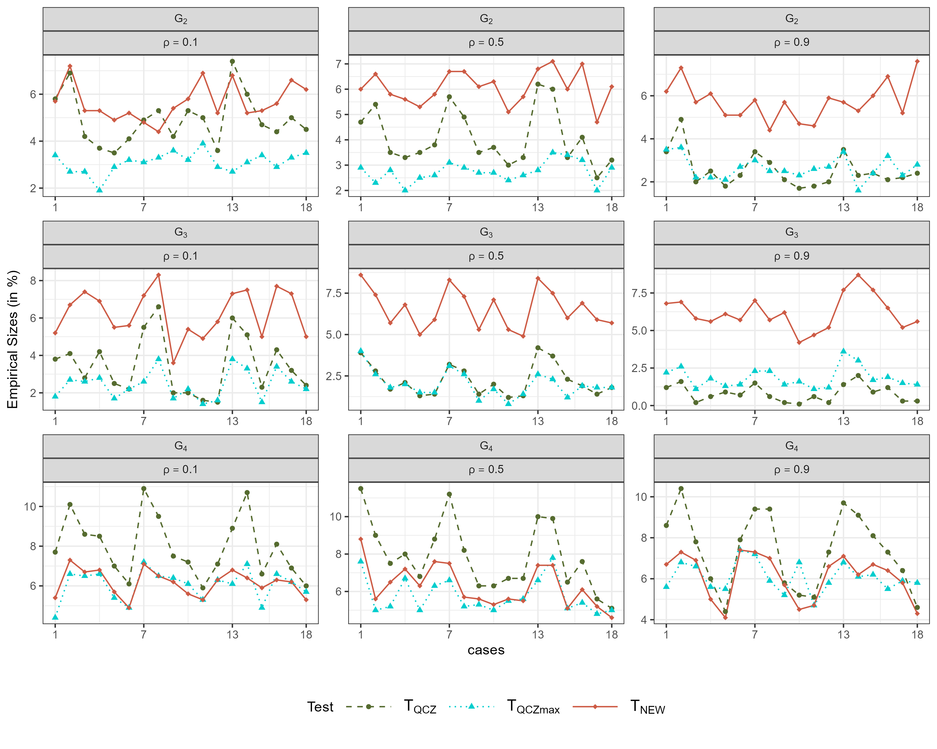
Figure 1: Simulation 1. The empirical sizes (in %) of $T_{QCZ}$, $T_{QCZ\max}$, and $T_{NEW}$ of H2 under different cases of $(\varepsilon_{ijr},{\bf\bm{\mathit{n}}},M)$. Cases 1–6: $\varepsilon_{ijr}\sim N(0,1)$ and the values of (${\bf\bm{\mathit{n}}},M$) are set as follows: 1.$({\bf\bm{\mathit{n}}}_{1},50)$, 2.$({\bf\bm{\mathit{n}}}_{1},100)$, 3.$({\bf\bm{\mathit{n}}}_{2},50)$, 4.$({\bf\bm{\mathit{n}}}_{2},100)$, 5.$({\bf\bm{\mathit{n}}}_{3},50)$, 6.$({\bf\bm{\mathit{n}}}_{3},100)$; Cases 7–12: $\varepsilon_{ijr}\sim t_{4}/\sqrt{2}$ with the same values of $({\bf\bm{\mathit{n}}},M)$ as in Cases 1–6; Cases 13–18: $\varepsilon_{ijr}\sim(\chi_{4}^{2}-4)/(2\sqrt{2})$ with the same values of $({\bf\bm{\mathit{n}}},M)$ as in Cases 1–6.

When the null hypothesis (3) of the GLHT problem is rejected, it is often of interest to further conduct some contrast tests. Now we are targeting to examine the finite-sample performance of $T_{NEW}$ of H2, that is, the two-sample problem for MFD. The empirical sizes (in %) of $T_{QCZ}$, $T_{QCZ\max}$, and $T_{NEW}$ are plotted in Figure 1. When the coefficient matrix ${\bf\bm{\mathit{G}}}$ is specified as ${\bf\bm{\mathit{G}}}_{2}$ (the first row in Figure 1), that is, we are comparing the two mean functions ${\bf\bm{\mathit{\eta}}}_{1}(t)$ and ${\bf\bm{\mathit{\eta}}}_{2}(t)$, $T_{NEW}$ performs well regardless of whether the simulated functional data are highly correlated ($\rho=0.1$), moderately correlated ($\rho=0.5$), or less correlated ($\rho=0.9$), since its empirical sizes are generally located around 5%. $T_{QCZ\max}$ is a bit conservative since most of its empirical sizes are located around 3%. $T_{QCZ}$ is comparable with $T_{NEW}$ when $\rho=0.1$, and slightly better than $T_{NEW}$ when $\rho=0.5$, but it is more conservative than $T_{NEW}$ when $\rho=0.9$. When ${\bf\bm{\mathit{G}}}={\bf\bm{\mathit{G}}}_{3}$, that is, we are comparing the two mean functions, ${\bf\bm{\mathit{\eta}}}_{1}(t)$ and ${\bf\bm{\mathit{\eta}}}_{3}(t)$, $T_{QCZ}$ and $T_{QCZ\max}$ are more conservative than $T_{NEW}$ when $\rho=0.5$ and 0.9. This is not surprising since $T_{QCZ}$ and $T_{QCZ\max}$ are proposed under the assumption of homogeneous covariance function holds. When $\rho=0.5$ and 0.9, this assumption was strongly invalid. However, this disadvantage can be overcome when the sample sizes of two groups are equal. When ${\bf\bm{\mathit{G}}}={\bf\bm{\mathit{G}}}_{3}$, that is, we are comparing the two mean functions, ${\bf\bm{\mathit{\eta}}}_{2}(t)$ and ${\bf\bm{\mathit{\eta}}}_{3}(t)$. Since we set $n_{2}=n_{3}$, it is seen from Figure 1, $T_{QCZ}$ and $T_{QCZ\max}$ are no more as conservative as the previous two cases.

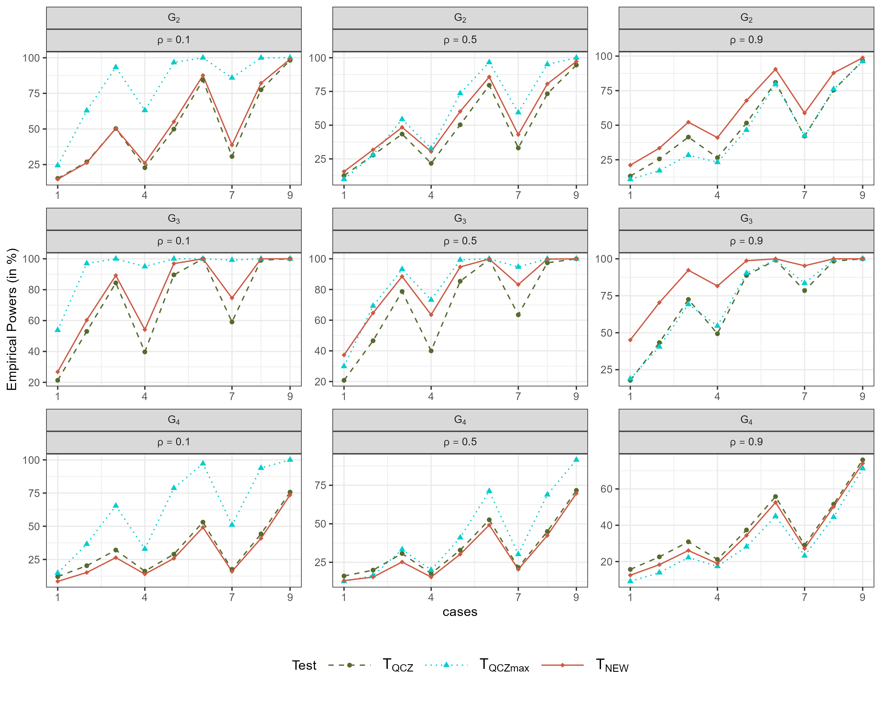
Figure 2: Simulation 1. The empirical powers (in %) of $T_{QCZ}$, $T_{QCZ\max}$, and $T_{NEW}$ of H2 when $\varepsilon_{ijr}\sim N(0,1)$ and $M=50$ under different cases of $(\delta,{\bf\bm{\mathit{n}}})$. For $\rho=0.1$, Cases 1–9 are as follows: 1.$(0.2,{\bf\bm{\mathit{n}}}_{1}$), 2.$(0.2,{\bf\bm{\mathit{n}}}_{2}$), 3.$(0.2,{\bf\bm{\mathit{n}}}_{3}$), 4.$(0.3,{\bf\bm{\mathit{n}}}_{1}$), 5.$(0.3,{\bf\bm{\mathit{n}}}_{2}$), 6.$(0.3,{\bf\bm{\mathit{n}}}_{3}$), 7.$(0.4,{\bf\bm{\mathit{n}}}_{1}$), 8.$(0.4,{\bf\bm{\mathit{n}}}_{2}$), 9.$(0.4,{\bf\bm{\mathit{n}}}_{3}$). For $\rho=0.5$, Cases 1–9 are as follows: 1.$(0.5,{\bf\bm{\mathit{n}}}_{1}$), 2.$(0.7,{\bf\bm{\mathit{n}}}_{2}$), 3.$(0.9,{\bf\bm{\mathit{n}}}_{3}$), 4.$(0.5,{\bf\bm{\mathit{n}}}_{1}$), 5.$(0.7,{\bf\bm{\mathit{n}}}_{2}$), 6.$(0.9,{\bf\bm{\mathit{n}}}_{3}$), 7.$(0.5,{\bf\bm{\mathit{n}}}_{1}$), 8.$(0.7,{\bf\bm{\mathit{n}}}_{2}$), 9.$(0.9,{\bf\bm{\mathit{n}}}_{3}$). For $\rho=0.9$, Cases 1–9 are as follows: 1.$(1.0,{\bf\bm{\mathit{n}}}_{1}$), 2.$(1.3,{\bf\bm{\mathit{n}}}_{2}$), 3.$(1.6,{\bf\bm{\mathit{n}}}_{3}$), 4.$(1.0,{\bf\bm{\mathit{n}}}_{1}$), 5.$(1.3,{\bf\bm{\mathit{n}}}_{2}$), 6.$(1.6,{\bf\bm{\mathit{n}}}_{3}$), 7.$(1.0,{\bf\bm{\mathit{n}}}_{1}$), 8.$(1.3,{\bf\bm{\mathit{n}}}_{2}$), 9.$(1.6,{\bf\bm{\mathit{n}}}_{3}$).

For saving space, we only plot the empirical powers (in %) of $T_{QCZ}$, $T_{QCZ\max}$, and $T_{NEW}$ of H2 for Gaussian functional data when $M=50$ in Figure 2. It is seen that when the functional data are highly correlated ($\rho=0.1$) and moderately correlated ($\rho=0.5$), $T_{QCZ\max}$ outperforms the other two tests, and $T_{NEW}$ and $T_{QCZ}$ are comparable. $T_{NEW}$ outperforms $T_{QCZ}$ and $T_{QCZ\max}$ when the simulated functional samples are less correlated $(\rho=0.9$) and the two sample sizes are different. Nevertheless, the application of $T_{NEW}$ is boarder compared to $T_{QCZ}$ and $T_{QCZ\max}$.

Last, we examine the finite-sample performance for a specific linear hypothesis, H3, via comparing it with the bootstrap based test $T_{BT}$. The empirical sizes of $T_{BT}$ and $T_{NEW}$ of H3 are presented in Table 3 with the last row displaying their ARE values associated the three cases of $\rho$. It is seen that $T_{BT}$ is rather conservative especially when $\rho$ is large. This observation highlights that the bootstrap based test dose not work well when dealing with the simulated functional data which are less correlated. In contrast, $T_{NEW}$ performs well regardless of whether the simulated functional samples are highly correlated, moderately correlated, or even less correlated.

Table 3: Simulation 1. Empirical sizes (in $\%$) of $T_{BT}$ and $T_{NEW}$ of H3.

			$\rho=0.1$		$\rho=0.5$		$\rho=0.9$
$\varepsilon_{ijr}$	${\bf\bm{\mathit{n}}}$	$M$	$T_{BT}$	$T_{NEW}$	$T_{BT}$	$T_{NEW}$	$T_{BT}$	$T_{NEW}$
$N(0,1)$	${\bf\bm{\mathit{n}}}_{1}$	50	4.7	6.0	4.1	7.2	1.6	5.6
		100	4.2	5.4	3.0	5.9	2.4	7.1
	${\bf\bm{\mathit{n}}}_{2}$	50	4.7	5.3	3.7	5.3	3.1	4.8
		100	4.6	5.3	3.6	4.4	2.4	4.1
	${\bf\bm{\mathit{n}}}_{3}$	50	4.9	5.7	4.3	5.4	2.5	4.0
		100	5.0	5.6	4.1	4.5	4.3	6.0
$t_{4}/\sqrt{2}$	${\bf\bm{\mathit{n}}}_{1}$	50	2.5	4.7	2.2	5.1	2.1	6.0
		100	4.4	6.8	2.6	5.0	1.7	5.8
	${\bf\bm{\mathit{n}}}_{2}$	50	4.1	4.8	3.7	5.7	3.7	5.5
		100	4.7	5.8	3.1	4.6	3.2	5.3
	${\bf\bm{\mathit{n}}}_{3}$	50	4.2	4.6	2.8	4.2	3.6	4.6
		100	4.0	4.5	4.9	6.1	4.3	5.5
$\frac{\chi_{4}^{2}-4}{2\sqrt{2}}$	${\bf\bm{\mathit{n}}}_{1}$	50	4.3	6.2	2.5	5.2	1.4	5.0
		100	4.0	6.2	4.1	6.2	2.0	5.6
	${\bf\bm{\mathit{n}}}_{2}$	50	4.2	4.8	3.8	5.1	3.3	5.4
		100	4.7	5.2	4.8	6.1	3.5	5.7
	${\bf\bm{\mathit{n}}}_{3}$	50	4.8	4.9	5.2	6.4	3.4	4.8
		100	4.4	4.7	5.7	5.8	4.4	6.3
ARE			12.89	11.67	26.22	14.22	41.22	13.89

In conclusion, we have conducted various hypothesis tests in this simulation by setting various coefficient matrix ${\bf\bm{\mathit{G}}}$. It shows that our proposed test $T_{NEW}$ works well no matter how the functional data correlated and does not require too large sample size to get the good performance. The broader applicability of $T_{NEW}$ suggests that it can be employed in a wider range of scenarios or research contexts beyond the specific framework proposed by Qiu et al. (2021) and Zhu et al. (2023). This flexibility allows researchers to adapt and use $T_{NEW}$ based on their specific needs and study designs.

3.2 Simulation 2

In this simulation study, we demonstrate the good performance of $T_{NEW}$ in more comprehensive and practical cases. As mentioned in Section 2.4, in practice, the functional data are usually observed at a grid of design time points and these time points may vary across different observations. In such a situation, it is necessary to initially reconstruct the functional data using a smoothing technique and subsequently discretize each reconstructed function at a shared set of design time points. The proposed global test then can be applied to the reconstructed data. We consider $k=4$ groups of multivariate functional samples with three vectors ${\bf\bm{\mathit{n}}}=[{\bf\bm{\mathit{n}}}_{1},{\bf\bm{\mathit{n}}}_{2},{\bf\bm{\mathit{n}}}_{3}]$ of sample sizes ${\bf\bm{\mathit{n}}}_{1}=[15,30,50,70]$, ${\bf\bm{\mathit{n}}}_{2}=[18,36,60,84]$, and ${\bf\bm{\mathit{n}}}_{3}=[24,48,80,112]$. The four functional observations are generated from the model which has been similarly considered by Górecki and Smaga (2017):

$${\bf\bm{\mathit{y}}}_{\alpha i}(t)={\bf\bm{\mathit{\eta}}}_{\alpha}(t)+{\bf\bm{\mathit{A}}}_{\alpha}(B_{1},B_{2})^{\top},\alpha=1,\ldots,4,$$ (16)

where ${\bf\bm{\mathit{A}}}_{1}=0.7{\bf\bm{\mathit{I}}}_{2}+0.3\bm{1}_{2}\bm{1}_{2}^{\top}$, ${\bf\bm{\mathit{A}}}_{2}=0.5{\bf\bm{\mathit{I}}}_{2}+0.5\bm{1}_{2}\bm{1}_{2}^{\top}$, ${\bf\bm{\mathit{A}}}_{3}=0.3{\bf\bm{\mathit{I}}}_{2}+0.7\bm{1}_{2}\bm{1}_{2}^{\top}$, ${\bf\bm{\mathit{A}}}_{4}=0.1{\bf\bm{\mathit{I}}}_{2}+0.9\bm{1}_{2}\bm{1}_{2}^{\top}$, and $B_{1}$ and $B_{2}$ are independent standard Brownian motions with dispersion parameter $0.2^{2}$. We aim to check the behavior of our proposed test $T_{NEW}$ against the tests proposed by Górecki and Smaga (2017), denoted as W, LH, P, and R, respectively, as well as $T_{ZZC}^{N}$ and $T_{ZZC}^{B}$ proposed by Zhu et al. (2023) under the following two scenarios:

• Model (16) with measurement error. That is, ${\bf\bm{\mathit{y}}}_{\alpha i}(t)={\bf\bm{\mathit{\eta}}}_{\alpha}(t)+{\bf\bm{\mathit{A}}}_{\alpha}(B_{1},B_{2})^{\top}+\bm{e}_{ij},\alpha=1,\ldots,4$, where $e_{ij\ell},\ell=1,2$ are i.i.d. normally random distributed random variables with mean zero and variance $\sigma^{2}$. We consider three cases of $\sigma=0.1,0.5$, and $0.9$.

• First, we generate the MFD from model (16). Then, for each observation, we randomly select $aM$ points from its value with $a=0.1,0.5$, and 0.9 to roughly generate sparse ($a=0.1$), semi-dense ($a=0.5$), and dense ($a=0.9$) MFD.

Note that for both S1 and S2, we first reconstruct individual functions by using smoothing splines, and then apply W, LH, P, R, $T_{ZZC}^{N}$, $T_{ZZC}^{B}$, and $T_{NEW}$ to the functional samples evaluated at the design time points specified in Simulation 1. Since all the competitors were proposed for the one-way FMANOVA problem (2), we set ${\bf\bm{\mathit{G}}}=[{\bf\bm{\mathit{I}}}_{3},-\bm{1}_{3}]$.

Table 4: Simulation 2. Empirical sizes (in $\%$) of W, LH, P, R, $T_{ZZC}^{N}$, $T_{ZZC}^{B}$, and $T_{NEW}$ under S1.

$\sigma$	${\bf\bm{\mathit{n}}}$	$M$	W	LH	P	R	$T_{ZZC}^{N}$	$T_{ZZC}^{B}$	$T_{NEW}$
0.1	${\bf\bm{\mathit{n}}}_{1}$	50	19.9	19.9	19.8	20.7	6.1	7.1	5.5
		100	19.8	19.7	19.8	19.8	6.0	7.1	5.4
	${\bf\bm{\mathit{n}}}_{2}$	50	17.6	17.7	17.6	18.3	5.6	6.6	5.3
		100	21.4	21.5	21.3	21.4	6.4	8.0	6.0
	${\bf\bm{\mathit{n}}}_{3}$	50	20.0	20.1	20.0	20.3	6.4	6.6	6.5
		100	20.2	20.2	20.2	20.9	7.0	7.7	5.5
0.5	${\bf\bm{\mathit{n}}}_{1}$	50	16.9	17.1	17.0	18.4	7.1	8.6	6.0
		100	20.3	20.3	20.2	21.1	5.5	7.5	5.0
	${\bf\bm{\mathit{n}}}_{2}$	50	14.7	14.6	14.7	14.6	5.2	6.8	4.2
		100	17.8	17.9	17.8	18.0	5.7	7.6	5.2
	${\bf\bm{\mathit{n}}}_{3}$	50	15.6	15.7	15.5	16.4	5.8	7.0	5.4
		100	20.7	20.8	20.4	22.2	5.8	7.0	5.6
0.9	${\bf\bm{\mathit{n}}}_{1}$	50	10.0	10.1	9.8	10.9	5.1	6.4	5.2
		100	16.1	16.0	16.0	16.9	4.8	6.3	5.0
	${\bf\bm{\mathit{n}}}_{2}$	50	10.3	10.2	10.0	10.8	6.0	7.2	4.1
		100	15.5	15.5	15.5	15.9	5.6	6.6	5.4
	${\bf\bm{\mathit{n}}}_{3}$	50	10.8	10.9	10.8	11.5	5.7	6.9	6.0
		100	15.3	15.4	15.4	17.1	6.2	7.1	5.5
ARE			236.56	237.33	235.33	250.22	18.22	42.33	11.33

The empirical sizes (in $\%$) of W, LH, P, R, $T_{ZZC}^{N}$, $T_{ZZC}^{B}$, and $T_{NEW}$ under S1 and S2 in Simulation 2 are displayed in Table 4 and Table 5, respectively, with the last row displaying their ARE values. We can get similar conclusions from these two tables. Firstly, it is apparent that all the tests proposed by Górecki and Smaga (2017) do not work well and they are rather liberal. $T_{ZZC}^{B}$ outperforms Górecki and Smaga (2017)’s tests but it is also a bit liberal. However, it is worth noting that $T_{ZZC}^{B}$ demonstrates better performance than those in Table 1. This is expected since this simulation study incorporates a larger number of observations and $T_{ZZC}^{B}$ can have a better performance if the sample size is large. $T_{ZZC}^{N}$ performs second and $T_{NEW}$ performs best. Hence, it can be concluded that $T_{NEW}$ remains effective even in scenarios where simulated functional samples exhibit measurement error or the simulated functional samples are sparse.

Table 5: Simulation 2. Empirical sizes (in $\%$) of W, LH, P, R, $T_{ZZC}^{N}$, $T_{ZZC}^{B}$, and $T_{NEW}$ under S2.

$a$	${\bf\bm{\mathit{n}}}$	$M$	W	LH	P	R	$T_{ZZC}^{N}$	$T_{ZZC}^{B}$	$T_{NEW}$
0.1	${\bf\bm{\mathit{n}}}_{1}$	50	11.9	12.1	11.8	13.0	4.9	8.1	5.1
		100	18.7	18.6	18.7	20.2	5.5	6.9	5.6
	${\bf\bm{\mathit{n}}}_{2}$	50	10.2	10.5	10.3	11.2	4.3	7.0	4.5
		100	19.3	19.6	19.4	19.3	4.8	6.4	4.6
	${\bf\bm{\mathit{n}}}_{3}$	50	12.4	12.4	12.3	13.0	4.9	7.2	6.0
		100	20.7	20.9	20.5	21.0	5.9	6.5	4.7
0.5	${\bf\bm{\mathit{n}}}_{1}$	50	22.1	22.1	22.2	22.4	6.4	8.6	5.6
		100	22.2	22.2	22.2	22.6	7.5	9.0	6.6
	${\bf\bm{\mathit{n}}}_{2}$	50	21.3	21.4	21.2	22.0	6.6	7.0	6.1
		100	21.6	21.7	21.4	22.1	6.4	7.7	6.2
	${\bf\bm{\mathit{n}}}_{3}$	50	19.4	19.2	19.4	18.7	5.6	5.8	4.9
		100	20.0	20.1	19.9	20.0	5.1	5.6	4.8
0.9	${\bf\bm{\mathit{n}}}_{1}$	50	21.8	21.8	21.8	22.8	5.6	7.9	5.8
		100	24.2	24.4	24.2	25.2	7.5	9.4	6.8
	${\bf\bm{\mathit{n}}}_{2}$	50	19.6	19.6	19.6	19.6	5.1	6.0	4.6
		100	22.5	22.5	22.8	23.2	6.1	6.7	5.7
	${\bf\bm{\mathit{n}}}_{3}$	50	21.7	21.7	21.7	22.2	7.5	8.7	6.4
		100	21.1	21.1	21.1	20.1	5.9	6.9	5.7
ARE			289.67	291.00	289.44	298.44	19.78	46.00	15.00

4 Real Data Applications

In this section, we apply W, LH, P, R, $T_{ZZC}^{N}$, $T_{ZZC}^{B}$, and $T_{NEW}$ to the financial data set which has been briefly described in Section 1. This financial data set contains the mean PD values aggregated by the economy of domicile and sector of each firm from 2012 to 2021. In particular, the number of firms in the four regions, that is, R1: Asia Pacific (Developed), R2: Asia Pacific (Emerging), R3: Eurozone, and R4: Non-Eurozone are 7, 10, 12, and 13, respectively. It is of interest to compare the mean aggregated PD curves corresponding to four important factors, namely, energy, financial, real estate, and industrial in the four regions are all the same. In data preparation, since the observed discrete multivariate functional observations are measured in different time points, we reconstruct individual functions by smoothing splines and re-evaluate them at the same design time points. Figure 3 displays the pointwise sample group mean functions and their 95% pointwise confidence bands of the four regions.

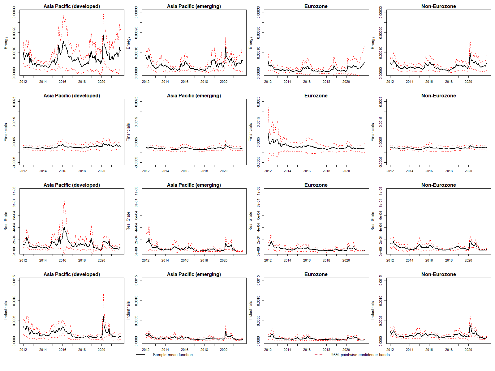
Figure 3: Group sample mean functions (solid) and their 95% pointwise confidence bands (dashed) of the smoothed PD values of energy, financial, real estate, and industrial of the firms in R1: Asia Pacific (Developed), R2: Asia Pacific (Emerging), R3: Eurozone, and R4: Non-Eurozone.

To check whether the underlying mean functions of the smoothed PD values of energy, financial, real estate, and industrial of the four regions are all the same, we apply W, LH, P, R, $T_{ZZC}^{N}$, $T_{ZZC}^{B}$, and $T_{NEW}$. The test results are shown in Table 6. Since all the considered tests suggest a strong rejection of the null hypothesis, we conclude that the underlying mean functions of the PD values of energy, financial, real estate, and industrial are unlikely the same for the four regions.

Table 6: Testing results for the financial data set.

	W	LH	P	R	$T_{ZZC}^{N}$	$T_{ZZC}^{B}$	$T_{NEW}$
Test Statistic	0.560	0.579	0.503	0.493	$30.68$	$30.68$	$11.19$
$p$-value	0.004	0.003	0.005	0.001	0.005	$<0.001$	$0.021$

Since the heteroscedastic one-way FMANOVA is highly significant, we further apply the tests under consideration to some contrast tests to check whether any two of the four regions have the same underlying groups mean functions of the PD values of energy, financial, real estate, and industrial. The tests results are given in Table 7. It is seen that all the tests give largely consistent conclusions. The contrast tests “R1 vs. R2”, “R1 vs. R4”, “R2 vs. R3” are significant but the contrast test “R1 vs. R3” is not significant. For the contrast test “R2 vs. R4”, W, LH, P, and $T_{ZZC}^{B}$ reject the null hypothesis, but R, $T_{ZZC}^{N}$ and $T_{NEW}$ do not reject the null hypothesis at the significance level 5%; For the contrast test “R3 vs. R4”, all the tests do not reject the null hypothesis except $T_{ZZC}^{B}$ at the significance level 5%. Based on our simulation results, it is evident that W, LH, P and $T_{ZZC}^{B}$ consistently exhibit liberal behavior. In contrast, our proposed new global test, $T_{NEW}$, outperforms its competitors in terms of size control. Consequently, the $p$-values generated by $T_{NEW}$ can be considered more reliable and trustworthy.

Table 7: $P$-values of W, LH, P, R, $T_{ZZC}^{N}$, $T_{ZZC}^{B}$, and $T_{NEW}$ for the financial data.

Hypothesis	W	LH	P	R	$T_{ZZC}^{N}$	$T_{ZZC}^{B}$	$T_{NEW}$
R1 vs. R2	0.009	0.006	0.014	0.002	$<0.001$	$<0.001$	$<0.001$
R1 vs. R3	0.607	0.608	0.609	0.551	0.329	0.270	0.447
R1 vs. R4	0.024	0.018	0.030	0.009	$<0.001$	$<0.001$	$<0.001$
R2 vs. R3	0.001	0.001	0.001	0.002	$<0.001$	$<0.001$	$0.004$
R2 vs. R4	0.027	0.031	0.023	0.051	0.080	$0.005$	$0.164$
R3 vs. R4	0.246	0.232	0.259	0.143	0.066	$0.009$	$0.077$

5 Concluding Remarks

In this paper, we propose and study a new global test for the general linear hypothesis testing problem for multivariate functional data. By adopting an adjustment coefficient, it controls the nominal size very well regardless of whether the functional data are nearly uncorrelated, moderately correlated, or highly correlated, and does not require a relative large sample size. The null limiting distribution of the proposed test is approximated using the three-cumulant matched chi-squared-approximation. Some simulation studies demonstrate that the proposed test generally outperforms the existing tests for multivariate functional data in terms of size control, and performs well not only for dense functional data but also for sparse ones.

APPENDIX: PROOFS

Proof of Theorem 1.

Let $\bar{{\bf\bm{\mathit{x}}}}_{\alpha}(t)$ is the usual vector of sample mean functions of ${\bf\bm{\mathit{x}}}_{\alpha i}$ defined in Condition C3. We can further rewrite $T_{n,0}^{*}$ in (8) as $T_{n,0}^{*}=\|{\bf\bm{\mathit{C}}}\bar{{\bf\bm{\mathit{x}}}}^{*}\|^{2}$ where $\bar{{\bf\bm{\mathit{x}}}}(t)=[\bar{{\bf\bm{\mathit{x}}}}_{1}(t)^{\top},\ldots,\bar{{\bf\bm{\mathit{x}}}}_{k}(t)^{\top}]^{\top}$ and $\bar{{\bf\bm{\mathit{x}}}}^{*}(t)=\bar{{\bf\bm{\mathit{x}}}}(t)[{\bf\bm{\mathit{I}}}_{p}\otimes{\bf\bm{\mathit{\Omega}}}_{n}^{-1/2}(t,t)]$. As $n_{\min}\to\infty$, by the central limit theorem of i.i.d. stochastic processes, we have $\bar{{\bf\bm{\mathit{x}}}}_{\alpha}(t)\stackrel{{\scriptstyle\mathcal{L}}}{{\longrightarrow}}\operatorname{GP}_{p}({\bf\bm{\mathit{0}}},{\bf\bm{\mathit{\Gamma}}}_{\alpha}/n_{\alpha})$, where $\operatorname{GP}_{p}(\bm{\eta},{\bf\bm{\mathit{\Gamma}}})$ denotes a $p$-dimensional Gaussian process with vector of mean functions $\bm{\eta}(t)$ and matrix of covariance functions ${\bf\bm{\mathit{\Gamma}}}(s,t)$. It follows that ${\bf\bm{\mathit{C}}}\bar{{\bf\bm{\mathit{x}}}}^{*}(t)\stackrel{{\scriptstyle\mathcal{L}}}{{\longrightarrow}}\operatorname{GP}_{kp}({\bf\bm{\mathit{0}}},{\bf\bm{\mathit{\Sigma}}})$ where ${\bf\bm{\mathit{\Sigma}}}(s,t)={\bf\bm{\mathit{C}}}\operatorname{diag}[{\bf\bm{\mathit{\Gamma}}}_{1}^{*}(s,t),\ldots,{\bf\bm{\mathit{\Gamma}}}_{k}^{*}(s,t)]{\bf\bm{\mathit{C}}}^{\top}$ with ${\bf\bm{\mathit{\Gamma}}}^{*}_{\alpha}(s,t)={\bf\bm{\mathit{\Omega}}}_{n}^{-1/2}(s,s){\bf\bm{\mathit{\Gamma}}}_{\alpha}(s,t){\bf\bm{\mathit{\Omega}}}_{n}^{-1/2}(t,t)/n_{\alpha}$. By applying Lemma 1 in Zhu et al. (2023), under Conditions C1–C3, we have $T_{0}^{*}\stackrel{{\scriptstyle d}}{{=}}\sum_{r=1}^{\infty}\lambda_{r}A_{r}$, where $A_{1},A_{2},\ldots\stackrel{{\scriptstyle\text{i.i.d.}}}{{\sim}}\chi_{1}^{2}$ and $\lambda_{1},\lambda_{2},\ldots$ are eigenvalues of ${\bf\bm{\mathit{\Sigma}}}(s,t)$ in descending order. It follows that $\mathcal{K}_{1}(T_{0}^{*})=\sum_{r=1}^{\infty}\lambda_{r}=\operatorname{tr}({\bf\bm{\mathit{\Sigma}}})$, $\mathcal{K}_{2}(T_{0}^{*})=2\sum_{r=1}^{\infty}\lambda_{r}^{2}=2\operatorname{tr}({\bf\bm{\mathit{\Sigma}}}^{\otimes 2})$, and $\mathcal{K}_{3}(T_{0}^{*})=8\sum_{r=1}^{\infty}\lambda_{r}^{3}=8\operatorname{tr}({\bf\bm{\mathit{\Sigma}}}^{\otimes 3})$. The last equality is given by

$$\begin{array}[]{rcl}&&\operatorname{tr}({\bf\bm{\mathit{\Sigma}}}^{\otimes 3})=\int_{\mathcal{T}^{3}}\operatorname{tr}[{\bf\bm{\mathit{\Sigma}}}(s,t){\bf\bm{\mathit{\Sigma}}}(t,v){\bf\bm{\mathit{\Sigma}}}(v,s)]dsdtdv\\ &=&\int_{\mathcal{T}^{3}}\operatorname{tr}\Big{\{}\Big{[}\sum\limits_{r_{1}=1}^{\infty}\lambda_{r_{1}}\bm{\phi}_{r_{1}}(s)\bm{\phi}_{r_{1}}(t)^{\top}\Big{]}\Big{[}\sum\limits_{r_{2}=1}^{\infty}\lambda_{r_{2}}\bm{\phi}_{r_{2}}(t)\bm{\phi}_{r_{2}}(v)^{\top}\Big{]}\Big{[}\sum\limits_{r_{3}=1}^{\infty}\lambda_{r_{3}}\bm{\phi}_{r_{3}}(v)\bm{\phi}_{r_{3}}(s)^{\top}\Big{]}\Big{\}}dsdtdv\\ &=&\sum\limits_{r_{1}=1}^{\infty}\sum\limits_{r_{2}=1}^{\infty}\sum\limits_{r_{3}=1}^{\infty}\int_{\mathcal{T}^{3}}\lambda_{r_{1}}\lambda_{r_{2}}\lambda_{r_{3}}\operatorname{tr}\left[\int_{\mathcal{T}^{3}}{\bf\bm{\mathit{\phi}}}_{r_{1}}(s){\bf\bm{\mathit{\phi}}}_{r_{1}}(t)^{\top}{\bf\bm{\mathit{\phi}}}_{r_{2}}(t){\bf\bm{\mathit{\phi}}}_{r_{2}}(v){\bf\bm{\mathit{\phi}}}_{r_{3}}(v){\bf\bm{\mathit{\phi}}}_{r_{3}}(s)^{\top}dsdtdv\right]\\ &=&\sum_{r=1}^{\infty}\lambda_{r}^{3}.\end{array}$$

The proof is then completed. ∎

Proof of Theorem 2. When $n_{\min}$ is large, we have $T_{n}/c_{n}=T_{n}^{*}[1+o(1)]$. Together with the local alternative (13) and the decomposition of $T_{n}^{*}$ in (8), this yields $T_{n}/c_{n}=\Big{\{}T_{n,0}^{*}+\int_{\mathcal{T}}\operatorname{tr}\left[{\bf\bm{\mathit{M}}}(t)^{\top}{\bf\bm{\mathit{H}}}{\bf\bm{\mathit{M}}}(t){\bf\bm{\mathit{\Omega}}}_{n}^{-1}(t,t)\right]dt\Big{\}}[1+o(1)].$ Theorem 1 indicates that as $n_{\min}\to\infty$, $T_{n,0}^{*}\stackrel{{\scriptstyle\mathcal{L}}}{{\longrightarrow}}\beta_{0}+\beta_{1}\chi_{d}^{2}$, then we have

$$\begin{split}&\quad\Pr\left[T_{n}/c_{n}\geq\widehat{\beta}_{0}+\widehat{\beta}_{1}\chi_{\widehat{d}}^{2}(\alpha)\right]\\ &=\Pr\left\{T_{n,0}^{*}\geq\widehat{\beta}_{0}+\widehat{\beta}_{1}\chi_{\widehat{d}}^{2}(\alpha)-\int_{\mathcal{T}}\operatorname{tr}\left[{\bf\bm{\mathit{M}}}(t)^{\top}{\bf\bm{\mathit{H}}}{\bf\bm{\mathit{M}}}(t){\bf\bm{\mathit{\Omega}}}_{n}^{-1}(t,t)\right]dt\right\}[1+o(1)]\\ &=\Pr\left\{\frac{\chi_{d}^{2}-d}{\sqrt{2d}}\geq\frac{\chi_{d}^{2}(\alpha)-d}{\sqrt{2d}}-\frac{n\int_{\mathcal{T}}\operatorname{tr}\left[{\bf\bm{\mathit{M}}}(t)^{\top}{\bf\bm{\mathit{H}}}^{*}{\bf\bm{\mathit{M}}}(t){\bf\bm{\mathit{\Omega}}}^{-1}(t,t)\right]dt}{\sqrt{2\sum_{\alpha=1}^{k}\sum_{\beta=1}^{k}h_{\alpha\beta}^{*2}\operatorname{tr}(\tilde{{\bf\bm{\mathit{\Gamma}}}}^{*}_{\alpha}\otimes\tilde{{\bf\bm{\mathit{\Gamma}}}}^{*}_{\beta})}}\right\}[1+o(1)].\\ \end{split}$$

where ${\bf\bm{\mathit{H}}}^{*}$, ${\bf\bm{\mathit{\Omega}}}(t,t),t\in\mathcal{T}$, and $\tilde{{\bf\bm{\mathit{\Gamma}}}}^{*}_{\alpha},\alpha=1,\ldots,k$ are defined in (14).

If $d\to\infty$, we have $(\chi_{d}^{2}-d)/\sqrt{2d}\to N(0,1)$ and $[\chi_{d}^{2}(\alpha)-d]/\sqrt{2d}\to z_{\alpha}$ where $z_{\alpha}$ denotes the upper $100\alpha$-percentile of $N(0,1)$. Thus, we have

$$\Pr\left[T_{n}/c_{n}\geq\widehat{\beta}_{0}+\widehat{\beta}_{1}\chi_{\widehat{d}}^{2}(\alpha)\right]=\Phi\left\{-z_{\alpha}+\frac{n\int_{\mathcal{T}}\operatorname{tr}\left[{\bf\bm{\mathit{M}}}(t)^{\top}{\bf\bm{\mathit{H}}}^{*}{\bf\bm{\mathit{M}}}(t){\bf\bm{\mathit{\Omega}}}^{-1}(t,t)\right]dt}{\sqrt{2\sum_{\alpha=1}^{k}\sum_{\beta=1}^{k}h_{\alpha\beta}^{*2}\operatorname{tr}(\tilde{{\bf\bm{\mathit{\Gamma}}}}^{*}_{\alpha}\otimes\tilde{{\bf\bm{\mathit{\Gamma}}}}^{*}_{\beta})}}\right\}[1+o(1)].$$

References

- Acal et al. (2022) Acal, C., A. M. Aguilera, A. Sarra, A. Evangelista, T. Di Battista, and S. Palermi (2022). Functional ANOVA approaches for detecting changes in air pollution during the COVID-19 pandemic. Stochastic Environmental Research and Risk Assessment 36(4), 1083–1101.
- Cuesta-Albertos and Febrero-Bande (2010) Cuesta-Albertos, J. and M. Febrero-Bande (2010). A simple multiway ANOVA for functional data. Test 19(3), 537–557.
- Cuevas et al. (2004) Cuevas, A., M. Febrero, and R. Fraiman (2004). An ANOVA test for functional data. Computational statistics & data analysis 47(1), 111–122.
- Duan et al. (2012) Duan, J.-C., J. Sun, and T. Wang (2012). Multiperiod corporate default prediction a forward intensity approach. Journal of Econometrics 170(1), 191–209.
- Górecki and Smaga (2017) Górecki, T. and Ł. Smaga (2017). Multivariate analysis of variance for functional data. Journal of Applied Statistics 44(12), 2172–2189.
- Qiu et al. (2021) Qiu, Z., J. Chen, and J.-T. Zhang (2021). Two-sample tests for multivariate functional data with applications. Computational Statistics & Data Analysis 157, 107160.
- Satterthwaite (1946) Satterthwaite, F. E. (1946). An approximate distribution of estimates of variance components. Biometrics bulletin 2(6), 110–114.
- Smaga and Zhang (2019) Smaga, Ł. and J.-T. Zhang (2019). Linear hypothesis testing with functional data. Technometrics 61(1), 99–110.
- Welch (1947) Welch, B. L. (1947). The generalization of ‘Student’s’ problem when several different population variances are involved. Biometrika 34(1/2), 28–35.
- Zhang (2005) Zhang, J.-T. (2005). Approximate and asymptotic distributions of chi-squared-type mixtures with applications. Journal of the American Statistical Association 100(469), 273–285.
- Zhang (2011) Zhang, J.-T. (2011). Two-way MANOVA with unequal cell sizes and unequal cell covariance matrices. Technometrics 53(4), 426–439.
- Zhang (2013) Zhang, J.-T. (2013). Analysis of variance for functional data. CRC press.
- Zhang and Chen (2007) Zhang, J.-T. and J. Chen (2007). Statistical inferences for functional data. The Annals of Statistics 35(3), 1052–1079.
- Zhang et al. (2019) Zhang, J.-T., M.-Y. Cheng, H.-T. Wu, and B. Zhou (2019). A new test for functional one-way ANOVA with applications to ischemic heart screening. Computational Statistics & Data Analysis 132, 3–17.
- Zhang and Liang (2014) Zhang, J.-T. and X. Liang (2014). One-way ANOVA for functional data via globalizing the pointwise F-test. Scandinavian Journal of Statistics 41(1), 51–71.
- Zhu et al. (2022) Zhu, T., J.-T. Zhang, and M.-Y. Cheng (2022). One-way MANOVA for functional data via Lawley–Hotelling trace test. Journal of Multivariate Analysis 192, 105095.
- Zhu et al. (2023) Zhu, T., J.-T. Zhang, and M.-Y. Cheng (2023). A global test for heteroscedastic one-way FMANOVA with applications. Journal of Statistical Planning and Inference. in press.