ASPEN: High-Throughput LoRA Fine-Tuning of Large Language Models with a Single GPU

Abstract.

Transformer-based large language models (LLMs) have demonstrated outstanding performance across diverse domains, particularly when fine-turned for specific domains. Recent studies suggest that the resources required for fine-tuning LLMs can be economized through parameter-efficient methods such as Low-Rank Adaptation (LoRA). While LoRA effectively reduces computational burdens and resource demands, it currently supports only a single-job fine-tuning setup.

In this paper, we present ASPEN, a high-throughput framework for fine-tuning LLMs. ASPEN efficiently trains multiple jobs on a single GPU using the LoRA method, leveraging shared pre-trained model and adaptive scheduling. ASPEN is compatible with transformer-based language models like LLaMA and ChatGLM, etc. Experiments show that ASPEN saves 53% of GPU memory when training multiple LLaMA-7B models on NVIDIA A100 80GB GPU and boosts training throughput by about 17% compared to existing methods when training with various pre-trained models on different GPUs. The adaptive scheduling algorithm reduces turnaround time by 24%, end-to-end training latency by 12%, prioritizing jobs and preventing out-of-memory issues.

1. Introduction

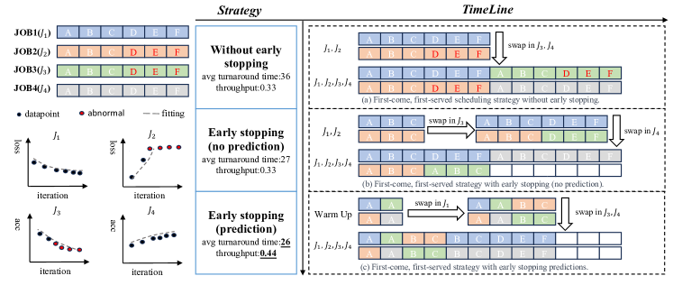
Figure 1. An example of adaptive job scheduling.

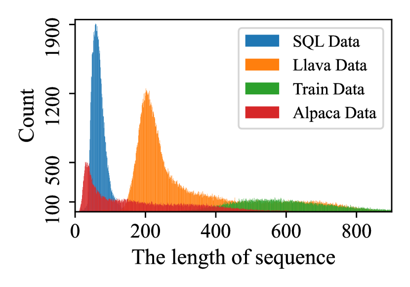
Figure 2. An example of a fused batch (the proportion of pad tokens is 25%) and distribution of various datasets.

Large language models (LLMs) have a significant impact on modern applications, expanding from natural language processing to a broader spectrum of domain-specific tasks, such as OpenAI-Chatgpt (openai-chatgpt, ), fine-tuned LLMs (touvron2023llama, ; vicuna2023, ; fastchat, ; du2022glm, ; touvron2023llama, ), and visual language models (alayrac2022flamingo, ; zhang2021vinvl, ). To adapt an LLM to multiple downstream applications, a common practice is to pre-train the model on large datasets, followed by fine-tuning it for applications (brown2020language, ; devlin2018bert, ; houlsby2019parameter, ; ouyang2022training, ).

Fine-tuning can be very expensive, typically requiring updates to all parameters of the pre-trained model (i.e., full-weight update), and the fine-tuned model may contain as many parameters as the pre-trained one (lv2023parameter, ). To overcome this, Low-Rank Adaptation (LoRA) (hu2021lora, ) enables efficient fine-tuning of a pre-trained model by creating small LoRA modules for different tasks. It is achieved by freezing the pre-trained model and only updating low-rank additive matrices, with much fewer parameters (than the pre-trained one).

LoRA greatly reduces the computational resources, making the fine-tuning process feasible across various tasks. For example, by the end of November 2023, thousands of LLaMA models (touvron2023llama, ) had been fine-tuned based on LoRA, accessible on the Hugging Face Hub (hugging-face, ). Further, on the HuggingFace Leaderboard (open-llm-leaderboard, ), 40% of the top 20 language models feature fine-tuning of the LLaMA model using LoRA and/or its derivatives. As of November 10, 2023, the highest-ranking LoRA-based model, GodziLLa2-70B (godzilla2-70b, ), is positioned 2nd, trailing the top-ranked LLM by only 1.67 points in the average performance evaluation score. These practical applications show that LoRA is not only extensively used for fine-tuning tasks in LLMs but also achieves high model accuracy comparable to other (full-weight) fine-tuning methods.

The extremely lightweight nature of LoRA-based fine tuning further allows for training multiple LoRA modules on a single commercial GPU. Intuitively, sharing a pre-trained model training among multiple training LoRA modules should bring the same benefits like reduced GPU memory usage and improved computation efficiency. However, a straightforward sharing approach – e.g., by only swapping in/out LoRA modules while keeping the pre-trained model in GPU memory when training multiple LoRA jobs – may introduce additional overheads, which could be suboptimal. Moreover, current LoRA-based fine-tuning systems, such as Alpaca-LoRA (alpaca-lora, ), predominantly concentrate on optimizing single-job fine-tuning and have not thoroughly investigated efficient strategies for fine-tuning multiple jobs.

In this paper, we present ASPEN, a high-throughput fine-tuning framework designed for training multiple LoRA fine-tuning jobs on a single GPU. ASPEN builds on top of a novel parallel fine-tuning approach called BatchFusion, which enables the concurrent training of multiple LoRA fine-tuning jobs and the sharing of pre-trained models by fusing multiple input batches into a single batch. Allocating system resources efficiently for multiple jobs is a complex task. Therefore, ASPEN incorporates a fine-grained, efficient job-level scheduler for handling multiple LoRA jobs. ASPEN has successfully tackled the following key issues:

In the BatchFusion process, when training data lengths vary, alignment is necessary and achieved by padding tokens to match the length of the longest data in the iteration. Figure 2 illustrates an example of a fused batch, with padding tokens occupying a significant proportion, resulting in lower overall throughput efficiency. Although these padding tokens do not directly impact model performance, their inclusion results in computational inefficiency. A key objective of ASPEN is to improve effective throughput by devising efficient padding strategies, thereby mitigating the computational inefficiencies arising from variable data lengths.

Training multiple LoRA fine-tuning jobs on a single GPU with limited resources requires significant resource management. As depicted in Figure 1 (left side), based on the loss or accuracy trends, $J_{2}$ and $J_{3}$ should be terminated early, as continuing to run those jobs with minimal gains consumes valuable compute resources without notable benefits. Moreover, maximizing resource usage also needs to limit training errors. For example, concurrently running too many jobs can maximize resource usage but risks out-of-memory errors. Dynamic allocation of resources, such as GPU memory, to each job is critical, yet predicting the exact memory needs during scheduling is challenging. ASPEN overcomes these challenges by developing delicate models to 1) predict when a job is unlikely to make further progress for early termination and 2) estimate the memory requirements of running jobs, avoiding out-of-memory errors.

To evaluate ASPEN, we fine-tuned several LLMs, including LLaMA-7B/13B (touvron2023llama1, ), ChatGLM2-6B (du2022glm, ), and LLaMA2-7B/13B(touvron2023llama, ). The results from these experiments highlight the efficiency of ASPEN in optimizing GPU utilization, GPU memory usage, and training throughput on a single GPU setup. When compared to Huggingface’s PEFT (peft, ), a leading parameter-efficient fine-tuning library employed by Alpaca-LoRA (alpaca-lora, ), QLoRA (dettmers2023qlora, ), and others, ASPEN showed a remarkable increase in throughput, achieving improvements of up to 17%. These findings underscore the potential of ASPEN as a robust tool for enhancing the efficiency and performance of LLMs in resource-constrained environments.

In summary, this paper has the following contributions:

1. We introduce the Multi-LoRA Trainer, enabling the efficient sharing of pre-trained model weights by BatchFusion method during the fine-tuning process of LLMs;

2. We propose the Adaptive Job Scheduler, which collects various metrics from jobs and enables the accurate estimation of both the performance of the model and resource utilization, maximizing the system efficiency;

3. ASPEN effectively uses computing resources, thereby improving training throughput and reducing training latency compared to state-of-the-art LoRA training systems. ASPEN saves 53% of GPU memory when training multiple LLaMA-7B models on NVIDIA A100 80GB GPU and boosts training throughput by about 17% compared to existing methods when training with various pre-trained models on different GPUs.

2. Background and Motivation

Fine-tuning pre-trained models. Training a large language model (LLM) from scratch requires substantial resources, both in terms of time and finances. It can take several days using thousands of GPUs (narayanan2021efficient, ) and entail significant financial investment (sharir2020cost, ). Fine-tuning pre-trained models has democratized the access of the advantages of LLMs: Many organizations make their pre-trained models publicly available, such as Meta’s LLaMA (touvron2023llama, ) and THUDM’s GLM (du2022glm, ). These pre-trained models can be fine-tuned for various downstream jobs – a method that has been proven effective (huang2020swapadvisor, ). Thus, leveraging these publicly accessible pre-trained models via fine-tuning becomes the most feasible way to harness the benefits of LLMs.

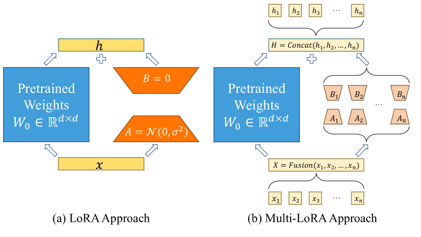
Figure 3. Sharing pre-trained model weights for training multiple LoRA jobs with reduced overhead.

Parameter-efficient fine-Tuning methods. A full-weight fine-tuning of large-scale pre-trained models typically needs to update all parameters of the models and is often associated with prohibitive computational costs (lv2023parameter, ). In contrast, parameter-efficient fine-tuning (PEFT) (peft, ) methods selectively fine-tune a few additional model parameters, resulting in substantial reductions in computational and memory resources. As one of the state-of-the-art PEFT techniques, LoRA (hu2021lora, ) achieves efficient fine-tuning by completely freezing the pre-trained model and introducing weight modifications through a trainable low-rank decomposition matrix, as illustrated in Figure 3(a) and expressed in Equation 1:

(1) $$h=W_{0}x+\Delta Wx=W_{0}x+BAx$$

where $x$ denotes the input batch of the fine-tune job, $W_{0}\in\mathbb{R}^{d\times k}$ represents the frozen pre-trained model weights, and $B\in\mathbb{R}^{d\times r}$ and $A\in\mathbb{R}^{r\times k}$ are low-rank decomposition matrices, with the rank $r\ll\text{min}(d,k)$.

Opportunities: sharing pre-trained models. Figure 3(a) illustrates a typical way to train a single LoRA fine-tuning job from a pre-trained model. When training multiple LoRA fine-tuning jobs using the same pre-trained model, sharing pre-trained models among all jobs seems intuitive to save GPU memory. A straightforward way to achieve this is by only swapping the low-rank matrices A and B for each job while keeping the pre-trained model in GPU memory. This way, multiple jobs are trained separately and sequentially meanwhile sharing the same pre-trained model. According to Equation 1, the matrix $x$ formed by the training data of each job is multiplied individually with the shared pre-trained model weights during the fine-tuning process of multiple LoRA jobs. Despite being simple, training multiple LoRA jobs sequentially may not be the most efficient approach in terms of resource utilization and training performance.

We have noted that the kernel launch cost incurred with each matrix multiplication and addition operation plays a substantial role in the overall training execution time. Further, we observed that if we can train multiple LoRA jobs in parallel, as shown in Figure 3(b), by “merging” individual jobs’ training data into a large matrix before multiplying it with the shared pre-trained model weights, the number of matrix multiplications can be reduced significantly (i.e., reduced launch costs), compared with the sequential training approach. Inspired by these observations, we propose a novel BatchFusion technique at §4.1.

Challenges: maximizing resource utilization. While training multiple LoRA jobs can more efficiently use computational resources and reduce training overhead, in scenarios with limited memory resources, running all jobs simultaneously is often impossible. The challenge then becomes how to schedule the running order of jobs to maximize the utilization of computational resources and improve system performance. Unlike other job scheduling algorithms (e.g., in operating systems), in the scenario of LoRA-based fine-tuning with multiple jobs, the memory usage of each job can be estimated in advance. Further, the early stopping prediction model makes the runtime of jobs predictable. This necessitates a scheduling algorithm that is more fitting for managing the scheduling of LoRA fine-tuning jobs.

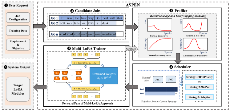
Figure 4. System overview of ASPEN.

3. System Overview

In this section, we present an overview of the ASPEN architecture and highlight its key design objectives.

Design objectives: ASPEN focuses on efficiently fine-tuning multiple LoRA jobs on a single GPU while effectively sharing pre-trained weights for these jobs. It dynamically schedules computational and memory resources for multiple LoRA jobs to optimize training throughput and resource utilization while maintaining model performance. The objectives of ASPEN are to answer the following two key questions:

• How can pre-trained weights be effectively shared with minimal overhead to enhance training throughput? (§4)

• How can we adaptively schedule jobs by estimating various metrics of training jobs to meet diverse requirements? (§5)

Architecture Overview: As illustrated in Figure 4, ASPEN consists of three main components:

• A self-supervised language model trainer that can handle multiple LoRA fine-tuning jobs, called the Multi-LoRA Trainer (❺);

• A profiler collecting various metrics of running jobs and producing estimated results for these metrics (❸);

• A job scheduler that can chooses a scheduling strategy based on the estimated results from the profiler and user requirements (❹).

ASPEN’s fine-tuning workflow: As depicted in Figure 4, users initiate requests to ASPEN (❶), providing hyperparameter configurations, training data, and scheduling objectives, which include minimizing waiting time, reducing turnaround time, maximizing throughput, among others, as elaborated in §5. Subsequently, ASPEN generates multiple candidate jobs (❷) based on this information and configures estimated fundamental parameters for each job in the Profiler (❸) during system initialization.

Once the system is initialized, the Scheduler (❹) selects a subset of jobs from the candidates, aligning them with user-defined scheduling objectives, and submits them to the Multi-LoRA Trainer (❺) for concurrent training. The Multi-LoRA Trainer (❺) provides performance metrics for the training jobs to the Profiler (❸) for estimation. The iteration of these steps (❸❹❺) constitutes one training cycle, repeated until all candidate jobs (❷) have completed their training.

In the event of new requests (❶) during training, ASPEN asynchronously generates candidate jobs (❷) based on the information provided in the requests. Subsequently, in the Profiler (❸), estimated fundamental parameters are configured for each job. The candidate job set is then updated before the commencement of the next iteration, ensuring that the training process incorporates the latest input seamlessly.

4. Multi-LoRA Trainer

In this section, we present the details of the Multi-LoRA Trainer, focusing on how it can efficiently share pre-trained weights across parallel LoRA fine-tuning jobs using a novel technique called BatchFusion. We then examine the costs associated with this approach. Further, we address a critical challenge encountered during the BatchFusion process, i.e., the issue of padding. To mitigate this, we introduce the OptimalBatch algorithm, aiming to minimize the impact of padding and optimize the overall fine-tuning process.

4.1. Batch Fusion

Unlike the existing model-sharing approach in training multiple LoRA fine-tuning jobs (stated in §3), we propose a novel BatchFusion technique for more efficient sharing a pre-trained model when training multiple LoRA fine-tuning jobs, as illustrated in Figure 3(b). BatchFusion fuses training data from multiple fine-tuning jobs into one batch before each training iteration; thus, multiple LoRA modules can share the same pre-trained model and participate in training in parallel in every iteration (instead of training sequentially or individually). The benefits of the proposed shared infrastructure are twofold: 1) It parallelizes the fine-tuning process by avoiding frequent swappings between fine-tuning jobs and mitigating model switching overhead. 2) It further optimizes the use of GPU resources by reducing kernel launch costs, thereby enhancing overall computational efficiency.

Specifically, the Multi-LoRA Trainer facilitates the parallel execution of multiple fine-tuning jobs on the same GPU. In Figure 3(b), consider multiple LoRA fine-tuning jobs, $J_{1},...,J_{n}$. Each job $J_{i}$ involves fine-tuning input data denoted as $x_{i}$. The low-rank decomposition matrices for the i-th job ($J_{i}$) are labeled as $A_{i}$ and $B_{i}$. Notably, all these jobs share the same pre-trained weights, represented by $W_{0}$. Formally, let $Fusion$ represent the BatchFusion process, and $Concat$ represent the matrices concatenation operation; the $Fusion$ operation is similar to matrix concatenation, but we add additional padding tokens to ensure dimension alignment, along with extra information to identify which LoRA module the input data belongs to. Thus, given the input batch for the i-th job $x_{i}$, the output data will be $h_{i}$. The fused batch matrix is $X=Fusion(x_{1},\dots,x_{n})$. It will be multiplied with the pre-trained weights and all LoRA module weights, and the individual results are then added together to produce the final output $H$. The complete calculation formula is shown as follows:

$$H =Concat(h_{1},\dots,h_{n})=W_{0}X+[\Delta W_{1}x_{1},\cdots,\Delta W_{n}x_{n}]$$

(2) $$=W_{0}X+[B_{1}A_{1}x_{1},\cdots,B_{n}A_{n}x_{n}]$$

where $W_{0}\in\mathbb{R}^{d\times k}$ denotes the shared pre-trained weights; $\Delta W_{i}=B_{i}A_{i}$ denotes the weights of the LoRA module trained by the i-th job, where $B_{i}\in\mathbb{R}^{d\times r_{i}}$ and $A_{i}\in\mathbb{R}^{r_{i}\times k}$ are low-rank decomposition matrices, with the rank $r_{i}\ll\text{min}(d,k)$.

4.2. Cost Analysis

To understand how the fusion of training data points from multiple fine-tuning jobs impacts the overall resource usage of the GPU, we analyze and evaluate the GPU memory usage and computation cost associated with the BatchFusion approach.

Memory cost. We observed that no popular system currently facilitates the sharing of pre-trained models for training multiple fine-tuning workloads. Therefore, we compare the GPU memory usage between the BatchFusion approach and the commonly used single-job LoRA fine-tuning system, i.e., Alpaca-LoRA (alpaca-lora, ). We assume 1) the weight of each individual LoRA model denoted as $W_{l}$, 2) the weight of the pre-trained base model represented as $W_{p}$, and 3) the additional memory required for training each LoRA model denoted as $W_{e}$. When running $k$ concurrent fine-tuning jobs on the same GPU, the total GPU memory required by the Alpaca-LoRA system (without BatchFusion) is $k(W_{p}+W_{l}+W_{e})$ – though running in parallel, each training job has its own copy of the pre-trained weight. In contrast, the BatchFusion approach reduces the need to replicate the pre-trained model weight $W_{p}$ for each job. Therefore, with $k$ jobs, BatchFusion saves $(k-1)W_{p}$ GB in GPU memory, thereby enhancing memory efficiency. As a concrete example, using quantized (e.g., 8-bit) LLaMA-7B models, BatchFusion can save the total memory amounting to $7(k-1)$ GB.

Computation cost. In GPU computation, before each operation, there is a need to launch the kernel to execute matrix multiplication and addition, and the overhead associated with this kernel launching can be nontrivial. This overhead is particularly impactful in the case of small kernels, i.e., kernels with computations for lower rank matrices (zhang2019understanding, ). This observation leads us to:

Fusing multiple small kernels into a large kernel can reduce overall computation costs by saving kernel launch costs; it can effectively reduce approximately 30% - 50% of the theoretical kernel launch costs. For example, given that PEFT (peft, ) is a widely used fine-tuning library employed by Alpaca-LoRA (alpaca-lora, ), QLoRA (dettmers2023qlora, ), and others, we analyze the computation cost for the Multi-LoRA Trainer and PEFT as below.

Assume there are $k$ LoRA fine-tuning jobs, each with a different training dataset. The input batch in each iteration can be denoted as $x_{1},\cdots,x_{k}$, and the fused batch $X=Fusion(x_{1},\cdots,x_{k})$. When running these $k$ LoRA fine-tuning jobs on a single GPU, the computation cost mainly includes kernel execution cost and kernel launch cost.

Kernel execution cost. According to Formulas (1, 4.1), the primary kernel execution cost involves matrix multiplication and addition operations. Because ASPEN does not introduce additional calculations, it shall have the same computational complexity as PEFT. Therefore, we consider the kernel execution cost of BatchFusion in ASPEN and the existing PEFT method to be the same.

Kernel launch cost. Since the fused batch $X$ is composed of multiple input batches $x_{i}$, it follows that $r(x_{i})<r(X)$. In computational operations involving matrix multiplication and addition, each operation initiates a kernel launch. As mentioned earlier, the overhead of kernel launches is particularly impactful for small kernels, i.e., kernels with computations for lower-rank matrices. Referring to Formulas (1, 4.1), the PEFT method requires $4k$ small kernel launches for $k$ fine-tuning jobs, each job involving three multiplications and one addition operation.

In contrast, the BatchFusion approach reduces the number of small kernel launches to $2k$, each with one multiplication operation. Additionally, it introduces two large kernel launches composed of an addition and a multiplication operation. Since the overhead of kernel launches for large kernels, i.e., kernels with computations for higher-rank matrices, is similar to that for small kernels, we infer that the total time spent on kernel launches is directly proportional to the number of launches. Therefore, the proposed BatchFusion approach effectively reduces the theoretical kernel launch costs by approximately $(2k-2)/4k$.

Summary. The BatchFusion approach devised in ASPEN can save $(k-1)W_{p}$ GB of GPU memory and approximately 30% to 50% of the kernel launch costs compared to the state-of-the-art PEFT method.

4.3. Data Alignment and Padding

In the BatchFusion process, when training data lengths vary, alignment is needed and achieved by adding padding tokens to match the length of the longest data in the iteration. Although these padding tokens do not directly affect model performance or the training process, their inclusion leads to computational inefficiency. This is because these tokens increase the volume of data processed without contributing to actual training, thereby using computational resources without benefiting the training effectiveness.

For instance, consider Figure 2, which depicts four fine-tuning jobs, each with a batch size of 2, amounting to six training data points. These data points vary in length, with the longest being six units. To align data lengths, padding tokens are appended to the shorter data points. Consequently, this leads to a less efficient use of computational resources.

Formally, we introduce the concept of the padding ratio, denoted as $\delta$, representing the proportion of the padding tokens in one batch. Let $\xi$ represent the total count of tokens in a fused batch, and $\xi_{p}$ represent the count of padding tokens in a fused batch. Then, $\delta$ is expressed as $\delta=\xi_{p}/\xi$. Notice that, for fine-tuning jobs sharing the same input training data, such as hyperparameter search scenarios, the training input data for each job is the same. Thus, we do not need to introduce padding tokens, and the $\delta$ is 0. On the other hand, in scenarios involving fine-tuning jobs addressing distinct domain issues (vicuna2023, ; jiao2023panda, ; xu2023baize, ; li2023chatdoctor, ; hu2023llmadapters, ), each job would use diverse training datasets. These datasets may have different length distributions, and thus the length of training data in each iteration will vary, resulting in a higher $\delta$. For exmaple, Figure 2 shows the distribution of data lengths for different datasets, which can significantly differ from each other.

We categorize the job throughput into two parts: the effective throughput and the non-effective throughput. Specifically, the non-effective throughput refers to the number of padding tokens computed by the system per second. The remaining part would be the effective throughput. Intuitively, a higher padding ratio would lead to worse effective throughput. Let $t$ represent the processing time, and $\sum token$ represent the total number of tokens processed in this period. $T_{tot}$ is the throughput, and the non-effective throughput $T_{non}$ and the effective throughput $T_{e}$ can be denoted as:

(3) $$T_{e}=T_{tot}-T_{non}=(1-\delta)T_{tot}=(1-\delta)\frac{\sum token}{t}$$

Therefore, our goal is to reduce the padding ratio $\delta$ while improving the effective throughput $T_{e}$.

Minimizing padding ratio. Drawing inspiration from Zhang et al. (zhang2021reducing, ), we introduce the OptimalBatch algorithm to minimize the padding ratio in training datasets. The optimal-batch algorithm executes the following key steps in each iteration of the training process: First, it sorts each job according to the length of its training data. Next, it selects either the shortest or the longest training data from each job. Finally, it employs the BatchFusion operation (as detailed in §4.1) to combine these selected training data. This fused data is then fed into the Multi-LoRA Trainer for processing.

However, this approach faces two main challenges: 1) Training models with sorted data can lead to issues with model performance convergence. As depicted in Figure 5, one can observe two distinct loss curves. The abnormal curve on the left exhibits fluctuating behavior, failing to show a clear trend toward convergence, in contrast to the stable and converging curve on the right. 2) Implementing this method requires all jobs to be stored in GPU memory to determine the optimal batching solution. It becomes problematic in memory-constrained environments, particularly when managing a large number of jobs, as it can lead to out-of-memory errors. A potential approach is to select a subset of jobs fitting within memory limits. However, identifying the most suitable subset for optimal results is nontrivial. Thus, we introduce the Job Scheduler to address these challenges in Section §5 .

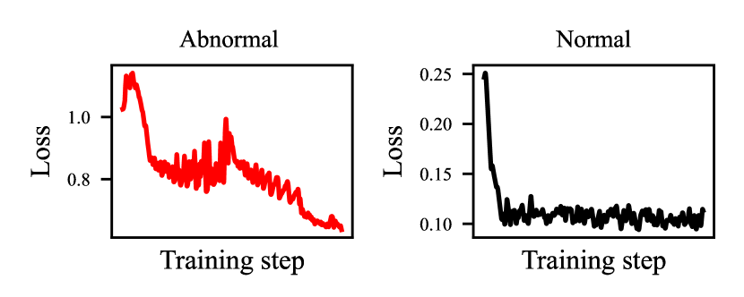
Figure 5. An abnormal loss curve and a normal loss curve.

5. Job Scheduler

In this section, we first present a near-optimal approach to reduce the impact of padding tokens on training throughput. We then introduce an adaptive job scheduling algorithm incorporating early stopping predictions and memory usage estimation models.

5.1. Optimizing Training Throughput

Scheduling multiple jobs in a memory-constrained environment, such as a single GPU, is challenging. Figure 6 shows an example where only two jobs can fit. Though FIFO is a common scheduling approach (mohan2022looking, ), it results in four padding tokens in the fused batch. In contrast, the $MinPad$ algorithm (our approach) reduces this to just one.

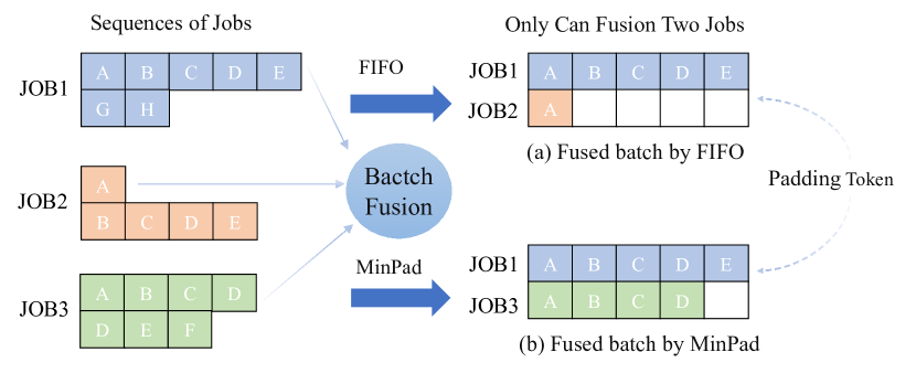
Figure 6. An example of the MinPad algorithm.

Observation: when handling numerous candidate jobs, selecting jobs with similar data length distributions for the same batch can reduce the padding ratio, thus improving effective throughput.

Based on this, we propose the $MinPad$ algorithm, to address the padding issues caused by BatchFusion: It first identifies the maximum number of jobs, $M$, that can be trained at the same time. Before each iteration, it reviews the data for each job and chooses $M$ training data with the fewest padding tokens. $MinPad$ correlates the execution order with the distribution of training data lengths. While $MinPad$ ensures the minimum padding ratio, maximizing effective throughput, and avoids the unconvergence of each training process caused by sorting, it does not consider the priority, turnaround time, and waiting time of jobs. The priority scheduling algorithm is often used to manage job priority (zouaoui2019priority, ), but this method does not consider the distribution of training data lengths, potentially increasing the padding ratio and reducing throughput, as discussed in §4.3.

5.2. Early Stopping and Throughput Modeling

In the model training process, if the model’s performance deteriorates or remains unchanged, early stopping can be employed to terminate the training prematurely (dodge2020fine, ). This approach avoids waiting to complete all training data, thus reducing unnecessary computation costs. As depicted in Figure 1, the lower-left corner displays the performance of four jobs during training. When calculating $J_{2}$’s loss value, a not-a-number ($NaN$) error occurs. If training persists, this error will recur, leading to abnormal model performance and wasted computing resources. $J_{3}$ and $J_{4}$ use various indicators to decide when to stop early. After each iteration, their accuracy is evaluated using a test set. $J_{3}$’s accuracy steadily declines during training, indicating that further training will not enhance performance and only waste resources. Therefore, it can be stopped early.

To simplify our discussion, we assume each iteration has a constant runtime, called iteration time. Four jobs, each with six iterations, were submitted concurrently. The system can run two jobs at once. Assuming equal priority for all four jobs, we compare three strategies: (a) a first-come, first-served scheduling strategy without early stopping; (b) a first-come, first-served strategy with early stopping; (c) a first-come, first-served strategy that includes both early stopping and a strategy that uses early stopping predictions for scheduling.

If we use strategy (a), six extra iterations will be done, wasting computational resources. Using strategy (b), the first step is to run $J_{1}$ and $J_{2}$ together. When $J_{2}$ encounters a $NaN$ error in its third iteration, it is stopped. Then, according to the first-come, first-served principle, $J_{3}$ starts running with $J_{1}$. After $J_{1}$ finishes, $J_{4}$ is scheduled to run alongside $J_{3}$.

Strategy (c) starts with a warm-up phase, where we run all jobs for two iteration times to gather prediction data. Then, scheduling is based on this data, prioritizing shorter jobs, $J_{2}$ and $J_{3}$, to increase throughput and reduce average turnaround time. In the given example, this method boosts throughput to 0.44 jobs per iteration time and lowers the average turnaround to 6.5 iterations per job.

Analysis between early stopping and throughout: To model the relationship between system throughput and early stopping, we consider a scenario where the total number of candidate jobs is $N$, and it is feasible to simultaneously run $k$ jobs. Each job involves $I_{i}$ iterations, and in the event of early stopping, the number of iteration times performed by each job is denoted as $L_{i}$, and the prediction accuracy is $\vartheta$. The set representing all training jobs is denoted as $\Gamma=\{L_{1},L_{2},\dots,L_{N}\}$. When utilizing prediction information for scheduling, the throughput is given by:

(4) $$T_{e}=\vartheta\frac{KN}{\sum_{i=1}^{N}L_{i}}$$

The optimal throughput remains the same as $T_{e}$ without prediction information. However, in the worst-case scenario, the throughput may decrease to:

(5) $$T_{w}=\frac{N}{\sum_{i=1}^{k}\top_{k}\Gamma}$$

Subsequently, we calculate its throughput as $T_{a}=(T_{e}+T_{w})/2$. The throughput improvement using early stopping prediction information for job scheduling is determined by:

(6) $$\eta_{tp}=\frac{T_{e}-T_{a}}{T_{a}}=\frac{\tau-1}{\tau+1}\quad(\tau=\frac{\vartheta k\sum_{i=1}^{k}\top_{k}\Gamma}{\sum_{i=1}^{N}L_{i}})$$

Equation 6 suggests that a larger difference in the actual number of iterations executed by each job results in a greater improvement in throughput. Thus, we can apply the early stopping prediction method, similar to estimating the risk at specific time points of gradient flow(ali2019continuous, ). This method can improve system throughput $\eta_{tp}$ and the higher the prediction accuracy $\vartheta$, the greater the throughput.

5.3. Fine-Tuning with Memory Usage Modeling

In the model training process, as depicted in Figure 2, there is an uneven distribution of data; varying input data lengths lead to different GPU memory requirements. The left column of Figure 7 shows that we fixed each job’s batch size to 24 and then adjusted the input data length to ascertain the maximum number of jobs that can run without encountering out-of-memory issues on a 48GB GPU.

Therefore, suppose that we know the amount of resources utilized by jobs in each step, it becomes possible to dynamically adjust the number of jobs that can be concurrently run. Initially, to estimate the resources required for each step of a job, we follow the previous work in Vijay et al. (korthikanti2023reducing, ) to infer the functional relationship between memory size and the size of input training data. Subsequently, we conduct online model fitting in the following manner: we define the input sequence length as $L_{n}$ and the input batch size as $B_{t}$. We can then employ the following model to capture this association:

(7) $$M=\beta_{0}+\beta_{1}B_{t}L_{n}+\beta_{2}B_{t}L_{n}^{2}$$

where $M$ represents the required memory, and $\beta_{0}$, $\beta_{1}$, and $\beta_{2}$ are non-negative coefficients. Throughout the model training process, we consistently gather data points $(B_{t},L_{n},M)$ and utilize a non-linear least squares solver to determine the optimal coefficients for fitting this model. An example of model fitting during the training of the LoRA model with LLaMA-7B is shown in Figure 7 (right column).

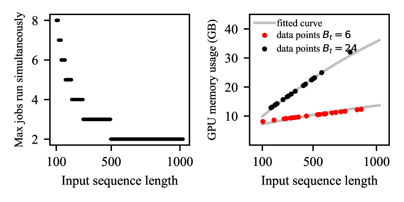
Figure 7. The maximum number of jobs that can run simultaneously with different input sequence lengths and online model fitting for training the LoRA model (with LLaMA-7B quantified in 8bit on NVIDIA RTX A6000 48GB) is determined by the coefficients $\beta_{0}=6.56$, $\beta_{1}=1.42\times 10^{-3}$, and $\beta_{2}=-8.76\times 10^{-8}$.

In ASPEN, we incorporate a warm-up phase before the actual training. This involves selecting data with various batch sizes and sequence lengths to fit Equation 7. At each step, we collect data points to enhance the accuracy of this model. With this estimated information, we can avoid out-of-memory issues by ensuring the following equation holds at each schedule:

(8) $$CS_{job}=\{X\mid X\subseteq S_{job}\land\textstyle\sum_{x\in X}x.m\leq M_{mem}\}$$

where $S_{job}$ denotes all available jobs for scheduling, $M_{mem}$ is the current maximum available memory, and $x.m$ signifies the estimated memory size derived from Equation 7. Equation 8 guarantees that the system prevents out-of-memory issues during runtime.

On the other hand, for efficient utilization of computational resources, we choose a set $S_{c}$ of jobs for concurrent execution. This set should ensure that the total memory of selected jobs is as close to $M_{mem}$ as possible. In other words, it should satisfy the following equation:

(9) $$S_{c}\subseteq CS_{job}\land(\forall S^{{}^{\prime}}\subseteq CS_{job},\textstyle\sum_{x\in S_{c}}x.m\geq\textstyle\sum_{x\in S^{{}^{\prime}}}x.m)$$

Algorithm 1 Adaptive Job Schedule

1:Job queue: $Q_{job}$, Maximum available memory: $M_{mem}$, User-defined parameter: $top\_k$

2:Scheduling result: R

3:$Q_{job}\leftarrow$ SortBy($Q_{job}$, priority, submitted_time)

4:$C_{job}\leftarrow$ GetFront($Q_{job}$, $top\_k$)

5:$C_{job}\leftarrow$ MemEstimate($C_{job}$)

6:$C_{job}\leftarrow$ EarlyStoppingPredict()

7:$C_{job}\leftarrow$ SortBy($C_{job}$, the_num_of_iterations) $\triangleright$ SJF

8:$R\leftarrow\emptyset$

9:for $x\in C_{job}$  do

10:     if GetMem($x$) + GetTotalMem($R$) $\leq$ $M_{mem}$ then

11:         $R\leftarrow R\cup x$

12:     end if

13:end for

5.4. Adaptive Job Scheduling

Based on early stopping prediction information and profile information on GPU memory, we propose an adaptive job scheduling to achieve: ❶ less waiting time, ❷ less turnaround time, ❸ large throughput, ❹ no out-of-memory issues, ❺ priority and fairness (high priority takes precedence, first come first serve). It is worth noting that the job scheduling problem is acknowledged as an NP problem (ullman1975np, ), and finding a solution that satisfies all the mentioned conditions is extremely challenging.

Taking inspiration from the operating system’s completely fair scheduling algorithms (kobus2009completely, ) and shortest job first algorithms (putra2020analysis, ), we present our adaptive job scheduling algorithm in Algorithm 1. This algorithm is designed to fulfill the aforementioned requirements as effectively as possible:

In step 1., to maximize the fulfillment of objective ❺, we employ a priority queue to rearrange jobs. They are sorted in descending order of priority. For jobs with the same priority, the one submitted earlier is placed at the front. In the next scheduling step, we select the top-k (where the user defines the parameter $top\_k$) jobs from the queue. Note that a job is removed from the queue only after its completion. In step 2., we use Equation 7 to estimate the resource requirements for each job among the top-k jobs. Then, by employing Equation 8, we can derive all feasible job scheduling methods that fulfill objective ❹. In step 3., using the predicted information, we estimate the number of iteration times needed to complete each job. Subsequently, we obtain the iteration time required for each job scheduling method. In step 4., to maximize the fulfillment of objectives (❶❷❸), we employ the Shortest Job First (SJF) (putra2020analysis, ) algorithm. This algorithm selects the scheduling method with the shortest time as the final scheduling result obtained from step 3.

During runtime, we optimize memory estimation and early stopping prediction models by collecting metric data through the profiler described in §3. Any changes in memory estimation results and early stopping prediction results will initiate a re-scheduling action.

6. Evaluation

6.1. Experimental Setup

Testbed. In our experiments, we employed four distinct graphics cards: the NVIDIA GeForce RTX 4090 24GB (rtx4090, ), NVIDIA RTX A6000 48GB (a6000, ), and NVIDIA A100 80GB(a100, ). We used five diverse models: the LLaMA1 (touvron2023llama, ) model with 7B and 13B parameters, the LLaMA2 model with 7B and 13B parameters, and the ChatGLM2 (du2022glm, ) with 6B parameters.

Workloads. For training the LoRA model, we employed two public datasets: AlpacaCleaned(alpaca, ) and Spider(yu2019spider, ). Each dataset obtained 90% of its data for training through a sampling method.

Baseline. We set up the commonly used single-job LoRA fine-tuning system, i.e., Alpaca-LoRA (alpaca-lora, ), as the baseline method. We compare system performance between ASPEN and using Alpaca-LoRA in two different ways. That is, Alpaca-Seq: training models sequentially, one after another, on a single GPU; Alpaca-Parallel: concurrently training multiple models on a single GPU. We also compared the impact of four different scheduling strategies on the system: the MinPad algorithm (name as $M3$) described in §5.1, FIFO scheduling algorithm (name as $M1$), priority scheduling algorithm (name as $M2$), and the adaptive scheduling algorithm (name as $M4$) described in §5.4.

Metrics. The evaluation focuses on the following key metrics: 1) Training Latency or Turnaround Time ($TT$): representing the end-to-end time required for model training; 2) Effective Throughput: quantifying the number of tokens (excluding padding tokens) trained per second, providing insight into training process efficiency; 3) GPU Memory Usage: assessing the amount of memory allocated during the training process on the GPU; 4) GPU Utilization Rate: the workload processed by the GPU within a specified time period; 5) Model Accuracy: evaluating model performance using the MMLU accuracy score (hendrycks2020measuring, ); 6) Waiting Time ($WT$): measuring the time spent waiting for the training job to start; 7) Virtual Turnaround Time ($VTT$): taking inspiration from the concept of virtual runtime in the Completely Fair Scheduler (CFS) algorithm (kobus2009completely, ), this metric is a normalized value of the real turnaround time, accounting for job priority. It is calculated as the product of the turnaround time and the priority, reflecting the accelerated virtual turnaround time for higher-priority jobs. For ease of representation, we normalized the time units and used $itime$ to denote time.

6.2. Performance Study

In end-to-end performance experiments, we employed the same dataset to train four LoRA models with varying learning rates, monitoring the number of tokens and padding tokens trained per second and calculating the effective throughput and non-effective throughput. Figure 8 illustrates the results, where the Ineffective portion represents non-effective throughput, and the others denote effective throughput. We compared (a) different models, (b) the same model architecture with different parameters and versions, and (c) the same model on different hardware. The training approach using ASPEN demonstrates a higher effective throughput by reducing kernel launch costs through BatchFusion operations and efficiently utilizing computational resources with job scheduling. The effective throughput has consistently improved by an average of 20%.

Memory saving. We compared the number of LoRA models that could be concurrently trained on a single A100 GPU using ASPEN and Alpaca-LoRA without encountering out-of-memory issues – we gradually increased the number of jobs until triggering an out-of-memory situation while recording their memory usage. Figure 9 shows that with the batch size 2, ASPEN trains 6x as many concurrent LoRA modules as Alpaca-LoRA; with batch sizes of 4 or 6, this number is 3x; with a batch size of 8, it is doubled. In the scenario of concurrently training the same number of LoRA models, ASPEN can save an average of about 53% of GPU memory compared to the approach without optimization.

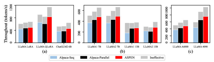
Figure 8. The throughput of (a) different models, (b) different parameters and versions, and (c) using different hardware.

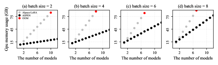
Figure 9. The GPU memory usage of Alpaca-LoRA and ASPEN with NVIDIA A100 80GB.

System resource utilization. ASPEN can efficiently utilize GPU computational resources and reduce memory usage. As shown in Figure 10, ASPEN has an average GPU utilization 1% higher than Alpaca-Parallel (with smaller fluctuations), while significantly reducing the average memory usage of jobs by sharing the pre-trained model. Thus, the job scheduling algorithm of ASPEN can effectively maintain GPU utilization at around 98%.

Early stopping. To illustrate the impact of early stopping, we analyze the latency and effective throughput of jobs using early stopping versus those without it. As shown in Figure 11, early stopping does not change the effective throughput, but saves end-to-end training latency: Both Alpaca-Parallel and ASPEN save 36% of the training latency, as this method avoids waiting for all training data to be completed.

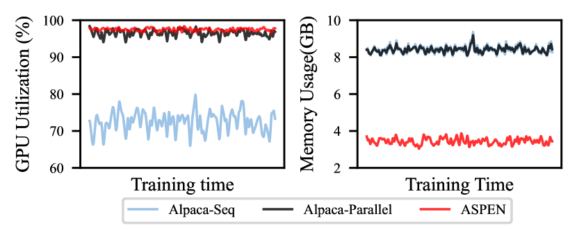
Figure 10. GPU utilization and memory usage.

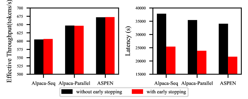
Figure 11. The effect of early stopping.

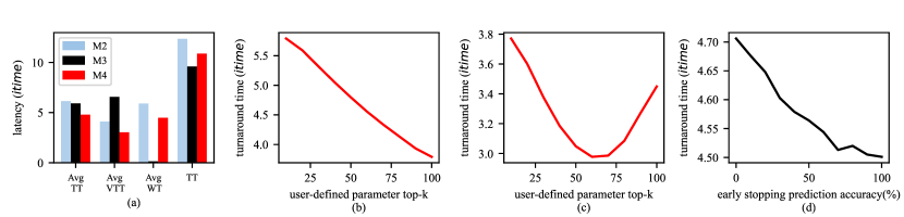
Figure 12. The effect of adaptive job scheduling.

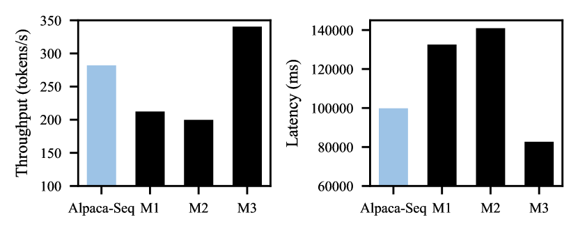
Figure 13. The effect of scheduling strategies.

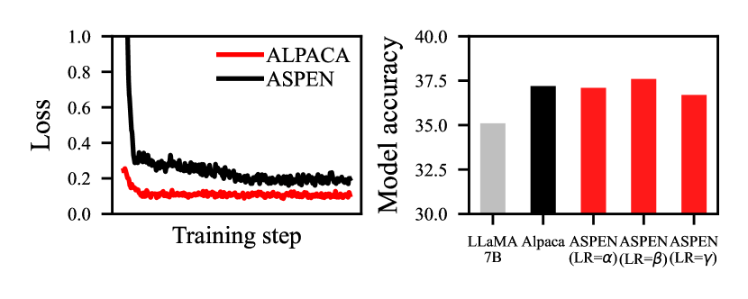
Figure 14. Loss curve and MMLU accuracy score under three different learning rates(LR): $\alpha=1\times 10^{-4}$, $\beta=2\times 10^{-4}$, $\gamma=5\times 10^{-5}$.

Effectiveness of MinPad. To demonstrate the effectiveness of MinPad scheduling strategies, we design the following experiments: we split the AlpacaCleaned and Spider datasets into eight subset datasets and trained eight LoRA models. Note that, Due to out-of-memory issues when training multiple models with LoRA-Parallel. We compare LoRA-Seq with MinPad ($M3$) and two other common scheduling algorithms: FIFO ($M1$) and priority ($M2$). Figure 13 shows that $MinPad$ improves the effective throughput by 21% and reduces end-to-end training latency by 17% compared to the baseline. However, for the other two scheduling strategies ($M1$ and $M2$), due to a lack of consideration of the padding issue, they result in a 30% decrease in both latency and effective throughput.

Effectiveness of adaptive job scheduler. To validate the effectiveness of the adaptive scheduling algorithm in achieving improved system performance, we analyze its impact on throughput, turnaround time, waiting time, job priority, and memory management. The experiment involved the simultaneous submission of 100 jobs with varying execution times, memory requirements, and priorities. These jobs underwent evaluation using three scheduling strategies: 1) Priority Scheduling ($M2$), 2) $MinPad$ Scheduling ($M3$) and 3) Adaptive Scheduling ($M4$).

Figure 12(a) illustrates that the $MinPad$ strategy minimizes end-to-end time ($TT$). However, it compromises job priorities, reflected in an average virtual turnaround time ($VTT$) twice that of the priority scheduling algorithm. The Adaptive Scheduling Algorithm integrates the benefits of the shortest job first algorithm, reducing average turnaround time, average waiting time ($WT$), and end-to-end latency. Compared to the baseline, it achieves a 24% reduction in turnaround time and a 12% decrease in end-to-end latency while ensuring job priorities. The performance of the adaptive scheduling algorithm is affected by the user-defined top-k value and the accuracy of early stopping predictions. Figure 12(d) shows that higher prediction accuracy correlates with reduced turnaround time. Figure 12(b, c) indicates that increasing the top-k value decreases turnaround time, approaching the $MinPad$ algorithm’s solution. However, this also entails a compromise on job priorities, as a smaller top-k value aligns the algorithm more closely with the priority scheduling approach, resulting in higher turnaround times.

Model convergence and performance. We trained three LoRA modules using the Alpaca-LoRA dataset and different learning rates with ASPEN and recorded the loss value for each iteration during the training process. Figure 14 (left side) shows that ASPEN and Alpaca-LoRA consistently ensure the convergence of model training. After training, we evaluated their accuracy score. As shown in Figure 14 (right side), the LoRA models trained by ASPEN exhibit accuracy almost identical to Alpaca, both about 2 points higher than LLaMA-7B. Thus, ASPEN does not affect the model’s performance and ensures the training process converges as expected.

7. Related Work

Fine-tuning of pre-trained models. Fine-tuning involves adapting models previously trained on extensive datasets to specific tasks. This is achieved by further training the model on a task-specific dataset, aiming to retain the knowledge of the pre-trained model while optimizing its response to the new task. An early example is Stanford Alpaca (alpaca, ), which employs a full fine-tuning approach, updating all model weights. In contrast, parameter-efficient fine-tuning methods like LoRA (hu2021lora, ), P-Turning (liu2023gpt, ), and LoRA’s derivatives including QLoRA (dettmers2023qlora, ), SoRA (ding2023sparse, ), LoftQ (li2023loftq, ), and AdaLoRA (zhang2023adaptive, ), among others, decrease resource demands while preserving performance. While our paper focuses on LoRA due to its wide adoption, most of its derivatives can be easily applied to our system.

Batching and reducing padding tokens. Batching enhances system throughput, especially in LLMs serving. S-LoRA (sheng2023slora, ), akin to ASPEN, utilizes Heterogeneous Batching to batch different LoRA adapters with varying ranks and share a pre-trained model when serving numerous LoRA adapters. vLLM (kwon2023efficient, ) reduces batch size by efficiently managing the KV cache, while FlexGen (sheng2023flexgen, ) allows a higher batch size upper bound through a new search space for offloading strategies. Approaches such as sorting inputs by length (zhang2021reducing, ) and token pruning (kim2022learned, ) aim to reduce padding tokens. Despite these significant contributions, these systems are optimized solely for serving scenarios and haven’t focused on training scenarios.

Early stopping. Predicting performance during training is addressed through regression. Ali et al. (ali2019continuous, ) explore statistical properties of iterates in gradient descent for least squares regression. Raskutti et al. (raskutti2014early, ) apply early stopping as regularization in non-parametric regression. Our profiler provides ample metric information, so these prediction methods can be easily incorporated into our system.

DL Model training resource estimation. Vijay et al. (korthikanti2023reducing, ) establish the functional relationship between memory size and input training data size. Yanjie et al. (10.1145/3368089.3417050, ) pre-built an analytic model for GPU memory consumption estimation. DLRover (wang2023dlrover, ) builds a prediction model for memory consumption in deep learning recommendation models. DNNPerf (gao2023runtime, ) builds a Graph Neural Network-based tool for predicting the runtime performance and memory consumption of deep learning models. However, these analytic approaches require extensive manual work and are limited to traditional model training. Our estimation approach is tailor-made for new multiple adapter scenes, thus achieving higher accuracy in this scene.

8. Conclusion

Transformer-based LLMs excel across domains, especially when fine-tuned for specific tasks. This paper introduces ASPEN, a high-throughput LoRA fine-tuning framework for LLMs on a single GPU. ASPEN employs LoRA to efficiently train multiple jobs by sharing pre-trained weights and using adaptive scheduling. Compatible with various LLMs like LLaMA and ChatGLM, ASPEN substantially increases training throughput by approximately 17% across different pre-trained weights and GPUs. The adaptive scheduling algorithm reduces turnaround time by 24% and end-to-end training latency by 12%, prioritizing jobs and preventing out-of-memory issues.

References

- (1) Jean-Baptiste Alayrac, Jeff Donahue, Pauline Luc, Antoine Miech, Iain Barr, Yana Hasson, Karel Lenc, Arthur Mensch, Katie Millican, Malcolm Reynolds, Roman Ring, Eliza Rutherford, Serkan Cabi, Tengda Han, Zhitao Gong, Sina Samangooei, Marianne Monteiro, Jacob Menick, Sebastian Borgeaud, Andrew Brock, Aida Nematzadeh, Sahand Sharifzadeh, Mikolaj Binkowski, Ricardo Barreira, Oriol Vinyals, Andrew Zisserman, and Karen Simonyan. Flamingo: A visual language model for few-shot learning. arXiv preprint arXiv:2204.14198, 2022.
- (2) Alnur Ali, J Zico Kolter, and Ryan J Tibshirani. A continuous-time view of early stopping for least squares regression. In The 22nd international conference on artificial intelligence and statistics, pages 1370–1378, 2019.
- (3) Edward Beeching, Clémentine Fourrier, Nathan Habib, Sheon Han, Nathan Lambert, Nazneen Rajani, Omar Sanseviero, Lewis Tunstall, and Thomas Wolf. Open llm leaderboard. https://huggingface.co/spaces/HuggingFaceH4/open_llm_leaderboard, 2023.
- (4) Tom B. Brown, Benjamin Mann, Nick Ryder, Melanie Subbiah, Jared Kaplan, Prafulla Dhariwal, Arvind Neelakantan, Pranav Shyam, Girish Sastry, Amanda Askell, Sandhini Agarwal, Ariel Herbert-Voss, Gretchen Krueger, Tom Henighan, Rewon Child, Aditya Ramesh, Daniel M. Ziegler, Jeffrey Wu, Clemens Winter, Christopher Hesse, Mark Chen, Eric Sigler, Mateusz Litwin, Scott Gray, Benjamin Chess, Jack Clark, Christopher Berner, Sam McCandlish, Alec Radford, Ilya Sutskever, and Dario Amodei. Language models are few-shot learners. arXiv preprint arXiv:2005.14165, 2020.
- (5) Wei-Lin Chiang, Zhuohan Li, Zi Lin, Ying Sheng, Zhanghao Wu, Hao Zhang, Lianmin Zheng, Siyuan Zhuang, Yonghao Zhuang, Joseph E. Gonzalez, Ion Stoica, and Eric P. Xing. Vicuna: An open-source chatbot impressing gpt-4 with 90%* chatgpt quality, March 2023.
- (6) NVIDIA Corp. Geforce rtx 4090. https://www.nvidia.com/en-us/geforce/graphics-cards/40-series/rtx-4090/, 2023.
- (7) NVIDIA Corp. Nvidia a100. https://www.nvidia.com/en-us/data-center/a100/, 2023.
- (8) NVIDIA Corp. Nvidia rtx a6000. https://www.nvidia.com/en-us/design-visualization/rtx-a6000/, 2023.
- (9) Tim Dettmers, Artidoro Pagnoni, Ari Holtzman, and Luke Zettlemoyer. Qlora: Efficient finetuning of quantized llms. arXiv preprint arXiv:2305.14314, 2023.
- (10) Jacob Devlin, Ming-Wei Chang, Kenton Lee, and Kristina Toutanova. Bert: Pre-training of deep bidirectional transformers for language understanding. arXiv preprint arXiv:1810.04805, 2018.
- (11) Ning Ding, Xingtai Lv, Qiaosen Wang, Yulin Chen, Bowen Zhou, Zhiyuan Liu, and Maosong Sun. Sparse low-rank adaptation of pre-trained language models. arXiv preprint arXiv:2311.11696, 2023.
- (12) Jesse Dodge, Gabriel Ilharco, Roy Schwartz, Ali Farhadi, Hannaneh Hajishirzi, and Noah Smith. Fine-tuning pretrained language models: Weight initializations, data orders, and early stopping. arXiv preprint arXiv:2002.06305, 2020.
- (13) Zhengxiao Du, Yujie Qian, Xiao Liu, Ming Ding, Jiezhong Qiu, Zhilin Yang, and Jie Tang. Glm: General language model pretraining with autoregressive blank infilling. In Proceedings of the 60th Annual Meeting of the Association for Computational Linguistics (Volume 1: Long Papers), pages 320–335, 2022.
- (14) Hugging Face. Hugging face. https://huggingface.co/, 2023.
- (15) Yanjie Gao, Xianyu Gu, Hongyu Zhang, Haoxiang Lin, and Mao Yang. Runtime performance prediction for deep learning models with graph neural network. In 2023 IEEE/ACM 45th International Conference on Software Engineering: Software Engineering in Practice (ICSE-SEIP), pages 368–380. IEEE, 2023.
- (16) Yanjie Gao, Yu Liu, Hongyu Zhang, Zhengxian Li, Yonghao Zhu, Haoxiang Lin, and Mao Yang. Estimating gpu memory consumption of deep learning models. In Proceedings of the 28th ACM Joint Meeting on European Software Engineering Conference and Symposium on the Foundations of Software Engineering, page 1342–1352, 2020.
- (17) Dan Hendrycks, Collin Burns, Steven Basart, Andy Zou, Mantas Mazeika, Dawn Song, and Jacob Steinhardt. Measuring massive multitask language understanding. arXiv preprint arXiv:2009.03300, 2020.
- (18) Neil Houlsby, Andrei Giurgiu, Stanislaw Jastrzebski, Bruna Morrone, Quentin De Laroussilhe, Andrea Gesmundo, Mona Attariyan, and Sylvain Gelly. Parameter-efficient transfer learning for nlp. In International Conference on Machine Learning, pages 2790–2799, 2019.
- (19) Edward J. Hu, Yelong Shen, Phillip Wallis, Zeyuan Allen-Zhu, Yuanzhi Li, Shean Wang, Lu Wang, and Weizhu Chen. Lora: Low-rank adaptation of large language models. arXiv preprint arXiv:2106.09685, 2021.
- (20) Zhiqiang Hu, Lei Wang, Yihuai Lan, Wanyu Xu, Ee-Peng Lim, Lidong Bing, Xing Xu, Soujanya Poria, and Roy Ka-Wei Lee. Llm-adapters: An adapter family for parameter-efficient fine-tuning of large language models. arXiv preprint arXiv:2304.01933, 2023.
- (21) Chien-Chin Huang, Gu Jin, and Jinyang Li. Swapadvisor: Pushing deep learning beyond the gpu memory limit via smart swapping. In Proceedings of the Twenty-Fifth International Conference on Architectural Support for Programming Languages and Operating Systems, pages 1341–1355, 2020.
- (22) Fangkai Jiao, Bosheng Ding, Tianze Luo, and Zhanfeng Mo. Panda llm: Training data and evaluation for open-sourced chinese instruction-following large language models. arXiv preprint arXiv:2305.03025, 2023.
- (23) Sehoon Kim, Sheng Shen, David Thorsley, Amir Gholami, Woosuk Kwon, Joseph Hassoun, and Kurt Keutzer. Learned token pruning for transformers. In Proceedings of the 28th ACM SIGKDD Conference on Knowledge Discovery and Data Mining, pages 784–794, 2022.
- (24) Jacek Kobus and Rafal Szklarski. Completely fair scheduler and its tuning. draft on Internet, 2009.
- (25) Vijay Anand Korthikanti, Jared Casper, Sangkug Lym, Lawrence McAfee, Michael Andersch, Mohammad Shoeybi, and Bryan Catanzaro. Reducing activation recomputation in large transformer models. Proceedings of Machine Learning and Systems, 5, 2023.
- (26) Woosuk Kwon, Zhuohan Li, Siyuan Zhuang, Ying Sheng, Lianmin Zheng, Cody Hao Yu, Joseph E. Gonzalez, Hao Zhang, and Ion Stoica. Efficient memory management for large language model serving with pagedattention. arXiv preprint arXiv:2309.06180, 2023.
- (27) Yixiao Li, Yifan Yu, Chen Liang, Pengcheng He, Nikos Karampatziakis, Weizhu Chen, and Tuo Zhao. Loftq: Lora-fine-tuning-aware quantization for large language models. arXiv preprint arXiv:2310.08659, 2023.
- (28) Yunxiang Li, Zihan Li, Kai Zhang, Ruilong Dan, Steve Jiang, and You Zhang. Chatdoctor: A medical chat model fine-tuned on a large language model meta-ai (llama) using medical domain knowledge. arXiv preprint arXiv:2303.14070, 2023.
- (29) Xiao Liu, Yanan Zheng, Zhengxiao Du, Ming Ding, Yujie Qian, Zhilin Yang, and Jie Tang. Gpt understands, too. arXiv preprint arXiv:2103.10385, 2023.
- (30) Kai Lv, Yuqing Yang, Tengxiao Liu, Qinghui Gao, Qipeng Guo, and Xipeng Qiu. Full parameter fine-tuning for large language models with limited resources. arXiv preprint arXiv:2306.09782, 2023.
- (31) Sourab Mangrulkar, Sylvain Gugger, Lysandre Debut, Younes Belkada, Sayak Paul, and Benjamin Bossan. Peft: State-of-the-art parameter-efficient fine-tuning methods. https://github.com/huggingface/peft, 2022.
- (32) Jayashree Mohan, Amar Phanishayee, Janardhan Kulkarni, and Vijay Chidambaram. Looking beyond gpus for dnn scheduling on multi-tenant clusters. In 16th USENIX Symposium on Operating Systems Design and Implementation (OSDI 22), pages 579–596, 2022.
- (33) Deepak Narayanan, Mohammad Shoeybi, Jared Casper, Patrick LeGresley, Mostofa Patwary, Vijay Korthikanti, Dmitri Vainbrand, Prethvi Kashinkunti, Julie Bernauer, Bryan Catanzaro, et al. Efficient large-scale language model training on gpu clusters using megatron-lm. In Proceedings of the International Conference for High Performance Computing, Networking, Storage and Analysis, pages 1–15, 2021.
- (34) OpenAI. Chatgpt [large language model]. https://chat.openai.com, 2023.
- (35) Long Ouyang, Jeffrey Wu, Xu Jiang, Diogo Almeida, Carroll Wainwright, Pamela Mishkin, Chong Zhang, Sandhini Agarwal, Katarina Slama, Alex Ray, et al. Training language models to follow instructions with human feedback. Advances in Neural Information Processing Systems, 35:27730–27744, 2022.
- (36) Maya Philippines. Godzilla2-70b. https://huggingface.co/MayaPH/GodziLLa2-70B, 2023.
- (37) Tri Dharma Putra. Analysis of preemptive shortest job first (sjf) algorithm in cpu scheduling. International Journal of Advanced Research in Computer and Communication Engineering, 9:41–45, 2020.
- (38) Garvesh Raskutti, Martin J Wainwright, and Bin Yu. Early stopping and non-parametric regression: An optimal data-dependent stopping rule. The Journal of Machine Learning Research, 15:335–366, 2014.
- (39) Or Sharir, Barak Peleg, and Yoav Shoham. The cost of training nlp models: A concise overview. arXiv preprint arXiv:2004.08900, 2020.
- (40) Ying Sheng, Shiyi Cao, Dacheng Li, Coleman Hooper, Nicholas Lee, Shuo Yang, Christopher Chou, Banghua Zhu, Lianmin Zheng, Kurt Keutzer, Joseph E. Gonzalez, and Ion Stoica. S-lora: Serving thousands of concurrent lora adapters. arXiv preprint arXiv:2311.03285, 2023.
- (41) Ying Sheng, Lianmin Zheng, Binhang Yuan, Zhuohan Li, Max Ryabinin, Daniel Y. Fu, Zhiqiang Xie, Beidi Chen, Clark Barrett, Joseph E. Gonzalez, Percy Liang, Christopher Ré, Ion Stoica, and Ce Zhang. Flexgen: High-throughput generative inference of large language models with a single gpu. arXiv preprint arXiv:2303.06865, 2023.
- (42) Rohan Taori, Ishaan Gulrajani, Tianyi Zhang, Yann Dubois, Xuechen Li, Carlos Guestrin, Percy Liang, and Tatsunori B. Hashimoto. Stanford alpaca: An instruction-following llama model, 2023.
- (43) Hugo Touvron, Thibaut Lavril, Gautier Izacard, Xavier Martinet, Marie-Anne Lachaux, Timothée Lacroix, Baptiste Rozière, Naman Goyal, Eric Hambro, Faisal Azhar, Aurelien Rodriguez, Armand Joulin, Edouard Grave, and Guillaume Lample. Llama: Open and efficient foundation language models. arXiv preprint arXiv:2302.13971, 2023.
- (44) Hugo Touvron, Louis Martin, Kevin Stone, Peter Albert, Amjad Almahairi, Yasmine Babaei, Nikolay Bashlykov, Soumya Batra, Prajjwal Bhargava, Shruti Bhosale, Dan Bikel, Lukas Blecher, Cristian Canton Ferrer, Moya Chen, Guillem Cucurull, David Esiobu, Jude Fernandes, Jeremy Fu, Wenyin Fu, Brian Fuller, Cynthia Gao, Vedanuj Goswami, Naman Goyal, Anthony Hartshorn, Saghar Hosseini, Rui Hou, Hakan Inan, Marcin Kardas, Viktor Kerkez, Madian Khabsa, Isabel Kloumann, Artem Korenev, Punit Singh Koura, Marie-Anne Lachaux, Thibaut Lavril, Jenya Lee, Diana Liskovich, Yinghai Lu, Yuning Mao, Xavier Martinet, Todor Mihaylov, Pushkar Mishra, Igor Molybog, Yixin Nie, Andrew Poulton, Jeremy Reizenstein, Rashi Rungta, Kalyan Saladi, Alan Schelten, Ruan Silva, Eric Michael Smith, Ranjan Subramanian, Xiaoqing Ellen Tan, Binh Tang, Ross Taylor, Adina Williams, Jian Xiang Kuan, Puxin Xu, Zheng Yan, Iliyan Zarov, Yuchen Zhang, Angela Fan, Melanie Kambadur, Sharan Narang, Aurelien Rodriguez, Robert Stojnic, Sergey Edunov, and Thomas Scialom. Llama 2: Open foundation and fine-tuned chat models. arXiv preprint arXiv:2307.09288, 2023.
- (45) Jeffrey D. Ullman. Np-complete scheduling problems. Journal of Computer and System sciences, 10:384–393, 1975.
- (46) Eric Wang. Alpaca-lora. https://github.com/tloen/alpaca-lora, 2023.
- (47) Qinlong Wang, Bo Sang, Haitao Zhang, Mingjie Tang, and Ke Zhang. Dlrover: An elastic deep training extension with auto job resource recommendation, 2023.
- (48) Canwen Xu, Daya Guo, Nan Duan, and Julian McAuley. Baize: An open-source chat model with parameter-efficient tuning on self-chat data. arXiv preprint arXiv:2304.01196, 2023.
- (49) Tao Yu, Rui Zhang, Kai Yang, Michihiro Yasunaga, Dongxu Wang, Zifan Li, James Ma, Irene Li, Qingning Yao, Shanelle Roman, Zilin Zhang, and Dragomir Radev. Spider: A large-scale human-labeled dataset for complex and cross-domain semantic parsing and text-to-sql task. arXiv preprint arXiv:1809.08887, 2019.
- (50) Lingqi Zhang, Mohamed Wahib, and Satoshi Matsuoka. Understanding the overheads of launching cuda kernels. ICPP19, pages 5–8, 2019.
- (51) Pengchuan Zhang, Xiujun Li, Xiaowei Hu, Jianwei Yang, Lei Zhang, Lijuan Wang, Yejin Choi, and Jianfeng Gao. Vinvl: Revisiting visual representations in vision-language models. In Proceedings of the IEEE/CVF conference on computer vision and pattern recognition, pages 5579–5588, 2021.
- (52) Qingru Zhang, Minshuo Chen, Alexander Bukharin, Pengcheng He, Yu Cheng, Weizhu Chen, and Tuo Zhao. Adaptive budget allocation for parameter-efficient fine-tuning. arXiv preprint arXiv:2303.10512, 2023.
- (53) Wei Zhang, Wei Wei, Wen Wang, Lingling Jin, and Zheng Cao. Reducing bert computation by padding removal and curriculum learning. In 2021 IEEE International Symposium on Performance Analysis of Systems and Software (ISPASS), pages 90–92, 2021.
- (54) Lianmin Zheng, Wei-Lin Chiang, Ying Sheng, Siyuan Zhuang, Zhanghao Wu, Yonghao Zhuang, Zi Lin, Zhuohan Li, Dacheng Li, Eric. P Xing, Hao Zhang, Joseph E. Gonzalez, and Ion Stoica. Judging llm-as-a-judge with mt-bench and chatbot arena. arXiv preprint arXiv:2306.05685, 2023.
- (55) Sonia Zouaoui, Lotfi Boussaid, and Abdellatif Mtibaa. Priority based round robin (pbrr) cpu scheduling algorithm. International Journal of Electrical & Computer Engineering (2088-8708), 9, 2019.