Asymptotic Theory of the Best-Choice Rerandomization using the Mahalanobis Distance

Abstract

Rerandomization, a design that utilizes pretreatment covariates and improves their balance between different treatment groups, has received attention recently in both theory and practice. There are at least two types of rerandomization that are used in practice: the first rerandomizes the treatment assignment until covariate imbalance is below a prespecified threshold; the second randomizes the treatment assignment multiple times and chooses the one with the best covariate balance. In this paper we will consider the second type of rerandomization, namely the best-choice rerandomization, whose theory and inference are still lacking in the literature. In particular, we will focus on the best-choice rerandomization that uses the Mahalanobis distance to measure covariate imbalance, which is one of the most commonly used imbalance measure for multivariate covariates and is invariant to affine transformations of covariates. We will study the large-sample repeatedly sampling properties of the best-choice rerandomization, allowing both the number of covariates and the number of tried complete randomizations to increase with the sample size. We show that the asymptotic distribution of the difference-in-means estimator is more concentrated around the true average treatment effect under rerandomization than under the complete randomization, and propose large-sample accurate confidence intervals for rerandomization that are shorter than that for the completely randomized experiment. We further demonstrate that, with moderate number of covariates and with the number of tried randomizations increasing polynomially with the sample size, the best-choice rerandomization can achieve the ideally optimal precision that one can expect even with perfectly balanced covariates. The developed theory and methods for rerandomization are also illustrated using real field experiments.

Keywords: potential outcome; randomization-based inference; optimal rerandomization; diverging number of covariates; Berry–Esseen bound

Introduction

Fisher (1925) advocated randomization in experimental design since it can eliminate bias and permit valid test of significance (Hall 2007). Since then, randomized experiments have become the gold standard for studying causal effects in many research areas, such as randomized clinical trials in medical research, randomized field experiments in social science, and online experiments in technology companies. The completely randomized experiment (CRE) has become one of the most popular designs due to its simplicity in both implementation and analysis. In addition, the CRE can balance all potential confounding factors, no matter observed or unobserved on average, and can justify simple and intuitive comparison between different treatment groups. For example, the difference between outcome means in two treatment groups, often called the difference-in-means estimator, is unbiased for the true average treatment effect (Neyman 1923).

However, as commented by Fisher (1926), most experimenters carrying out random assignments of plots will be shocked to find out how far from equally the plots distribute themselves, and more recently by Morgan and Rubin (2012), with $10$ mutually independent covariates and at $5\%$ significance level, the usual covariate balance test will be significant for at least one covariate with probability about $40\%$. Note that the covariate balance test has become a common practice when reporting randomized experiments nowadays. When chance imbalances are observed, researchers may worry about the results from the experiment, since the difference between the treatment groups in comparison may be to due to the difference in pretreatment covariates. Technically speaking, this is related to the variability of the treatment effect estimation, and, as we demonstrate later, we can reduce the variability of the treatment effect estimator or equivalently enhance its precision by improving the balance of pretreatment covariates.

The classical solution to avoiding chance imbalance of pretreatment covariates is blocking (Fisher 1935; Box et al. 2005), which, however, works mainly when we only have a few discrete covariates. Through a survey of leading researchers carrying out randomized experiments in developing countries, Bruhn and McKenzie (2009) discovered several rerandomization methods that are used in practice to improve covariate balance but are not well discussed in print. Rerandomization turns out to provide a general solution to the covariate balance issue, which can easily accommodate many covariates of various types. Although its idea has existed for a long time in the literature tracing back to Fisher (Savage 1962, Page 88), Gosset Student (1938), Cox Cox (1982) and etc., the rerandomization design is formally proposed until recently by Morgan and Rubin (2012), who also adopted and advocated the Fisher randomization test to analyze such a design. As discussed in Bruhn and McKenzie (2009), there are at least two types of rerandomization: the first specifies a certain covariate balance criterion and keeps drawing treatment assignments until getting an acceptable one, and the second draws, say, $1000$, randomizations and chooses the one with the best covariance balance based on a certain covariate imbalance measure. Both of them are intuitive designs and have been commonly used in practice, but their analysis is not straightforward compared to the classical and well-studied CRE. Recently Li et al. (2018) studied the large-sample theory for the first type of rerandomization, revealing a general non-Gaussian asymptotic distribution for the usual difference-in-means estimator; see, e.g., Li and Ding (2020); Li et al. (2020); Yang et al. (2021); Zhao and Ding (2021); Wang et al. (2021); Lu et al. (2022); Cohen and Fogarty (2022); Branson et al. (2022); Wang and Li (2022) for related extensions.

In this paper we will focus on the second type of rerandomization, which randomizes the treatment assignment multiple times and chooses the one with the best covariate balance, and, to distinguish it from the first type, we will call it the best-choice rerandomization. The best-choice rerandomization has received less attention in theory, despite its popularity in practice. Our goal is to address this theoretical gap by developing the large-sample theory and inference for the best-choice rerandomization. Specifically, we will consider the best-choice rerandomization design that draws $T\geq 1$ complete randomizations and chooses the one with the smallest covariate imbalance measured by the Mahalanobis distance, which is one of the most popular imbalance measure for multivariate covariates. A general procedure of a best-choice rerandomization is illustrated using the diagram in Figure 1, in parallel with Morgan and Rubin (2012, Figure 1) for the first type of rerandomization. Specifically, we first randomly and independently draw treatment assignments $T$ times, then calculate the covariate balance for each of these assignments based on some prespecified measure, and finally choose the one with the best balance and use that to conduct the actual experiment.

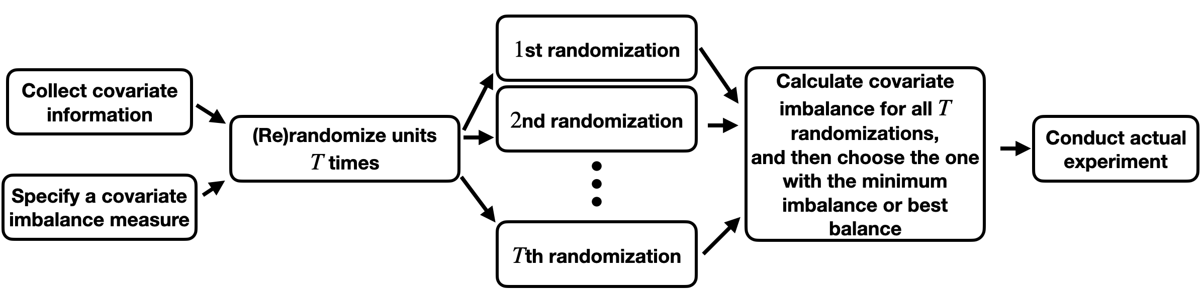
Figure 1: A general procedure of the best-choice rerandomization design.

Compared to the first type of rerandomization that discards assignments with bad covariate balance, the best-choice rerandomization has at least two salient features that can overcome some drawbacks of the first type. First, when the prespecified covariate balance criterion is too stringent, it is possible that no assignment will be acceptable under the first type of rerandomization. Second, even if there are acceptable assignments, it may take a long, random, and thus uncertain computation time to get an acceptable assignment for the first type of rerandomization. In contrast, the best-choice rerandomization can always produce a feasible assignment, and can always get that in a prespecified time. Despite these, it is not clear from the existing literature that how a proper statistical inference can be conducted for the best-choice rerandomization. Note that, following Morgan and Rubin (2012), we can still use Fisher randomization test, but it will work only for sharp null hypotheses that generally requires constant-effect-type assumptions or more broadly bounded null hypotheses that typically focus on the extreme individual effect (Caughey et al. 2023). In this paper, we will instead focus on Neyman (1923)’s large-sample repeated sampling inference for the average treatment effect, allowing unknown individual effect heterogeneity, and demonstrate the advantage of rerandomization over complete randomization. We also want to point out that the main purpose of this paper is not to compare the two types of rerandomization, but rather to provide large-sample inference tools for practitioners that design and analyze experiments from the second type of rerandomization.

Another question that will receive special attention in our paper is the choice of $T$, the number of tried complete randomizations. Intuitively, larger $T$ can provide greater covariate balance and seems an attractive option for practitioners. However, when $T$ is overly large and in particular is infinite in the extreme case, all possible treatment assignments will be enumerated and the best-choice rerandomization will essentially choose the one with the best balance from all possible assignments. When some covariates are continuous, this will generally lead to an almost deterministic design where there is no randomness in the treatment assignment. This apparently violates Fisher’s principle of experimental design. A natural question to ask is then: how large can and should $T$ be so that (i) there is still sufficient randomness in the treatment assignment for robust causal inference and (ii) rerandomization can achieve an “optimal” efficiency for treatment effect estimation? To the best of our knowledge, the choice of $T$ has been theoretically investigated only recently by Banerjee et al. (2020), from an ambiguity-averse decision-making perspective. Specifically, the authors considered an $\varepsilon$-contamination-type model (Huber 1964), which essentially allows model or prior misspecification, to facilitate the discussion on the trade-off between subjective expected performance and robust performance guarantees. They found that the loss in robustness due to rerandomization is of order $O(\sqrt{\log(T)/n})$, with $T$ denoting the number of tried complete randomizations and $n$ denoting the number of experimental units, and suggested choosing $K$ less than the sample size $n$, ensuring the loss is on the order of $O(\sqrt{\log(n)/n})$. We will also study the same issue on the choice of $T$, but from a different perspective. In particular, we will focus on the feasibility of a large-sample randomization-based robust inference for treatment effects. In addition, we will also investigate the role of the number of covariates $K$ in rerandomization.

The paper proceeds as follows. Section 2 introduces the framework and notation. Section 3 studies the asymptotic properties of the best-choice rerandomization. Section 4 investigates whether the best-choice rerandomization can achieve its ideally optimal precision that one can expect even with perfectly balanced covariates. Section 5 proposes large-sample valid inference for the best-choice rerandomization. Section 6 conducts simulations to illustrate our theory, and Section 7 concludes with a short discussion.

Framework and Notation

2.1 Potential outcomes, covariates and treatment assignments

Consider an experiment with $n$ units, where $n_{1}$ of them will receive some active treatment and the remaining $n_{0}=n-n_{1}$ will receive control. We invoke the potential outcome framework to define treatment effects (Neyman 1923; Rubin 1974). For each unit $1\leq i\leq n$, let $Y_{i}(1)$ and $Y_{i}(0)$ denote the treatment and control potential outcomes, and $\tau_{i}=Y_{i}(1)-Y_{i}(0)$ be the corresponding individual treatment effect. We are interested in inferring the average treatment effect $\tau=n^{-1}\sum_{i=1}^{n}\tau_{i}=\bar{Y}(1)-\bar{Y}(0)$, where $\bar{Y}(1)=n^{-1}\sum_{i=1}^{n}Y_{i}(1)$ and $\bar{Y}(0)=n^{-1}\sum_{i=1}^{n}Y_{i}(0)$ denote the average treatment and control potential outcomes, respectively. The fundamental difficulty of causal inference is that we can observe at most one potential outcome for each unit and thus half of the potential outcomes will be missing. Specifically, for each unit $i$, let $Z_{i}\in\{0,1\}$ be the treatment assignment indicator, where $Z_{i}=1$ if the unit receives treatment and $0$ otherwise. The observed outcome for each unit $i$ is then $Y_{i}=Z_{i}Y_{i}(1)+(1-Z_{i})Y_{i}(0)$, one of the two potential outcomes.

Throughout the paper, we will conduct the randomization-based inference (Neyman 1923; Li and Ding 2017), also called the design-based or finite population inference, where all the potential outcomes (as well as the pretreatment covariates introduced shortly) for the $n$ experimental units are viewed as fixed constants or equivalently being conditioned on. The finite population inference has the advantage of avoiding any model or distributional assumptions on the potential outcomes and covariates (as well as their dependence structure). The randomness in the observed data comes solely from the random treatment assignment. Therefore, the distribution of the treatment assignment vector $\boldsymbol{Z}=(Z_{1},Z_{2},\ldots,Z_{n})^{\top}$, also called the treatment assignment mechanism (Rubin 1978), governs the data generating process and is crucial for statistical inference. In a randomized experiment, the experimenter can generate the treatment assignment vector from a carefully prespecified or designed distribution, based on which units will be allocated into treatment and control groups.

The completely randomized experiment (CRE) is one of the most commonly used treatment assignment mechanism, under which the treatment assignment vector $\boldsymbol{Z}$ takes a particular value $\boldsymbol{z}=(z_{1},z_{2},\ldots,z_{n})^{\top}\in\{0,1\}^{n}$ with probability $\binom{n}{n_{1}}^{-1}$ if $\sum_{i=1}^{n}z_{i}=n_{1}$ and zero otherwise.

2.2 Covariate imbalance and rerandomization

Let $\boldsymbol{x}_{i}\in\mathbb{R}^{K}$ denote the available pretreatment covariate vector for each unit $i$, $\bar{\boldsymbol{x}}=n^{-1}\sum_{i=1}^{n}\boldsymbol{x}_{i}$ denote the average covariate vector for all units, and $\boldsymbol{S}^{2}_{\boldsymbol{x}}=(n-1)^{-1}\sum_{i=1}^{n}(\boldsymbol{x}_{i}-\bar{\boldsymbol{x}})(\boldsymbol{x}_{i}-\bar{\boldsymbol{x}})^{\top}$ denote the finite population covariance matrix of covariates. We further introduce

$$\hat{\boldsymbol{\tau}}_{\boldsymbol{x}}=\bar{\boldsymbol{x}}_{1}-\bar{\boldsymbol{x}}_{0}=\frac{1}{n_{1}}\sum_{i=1}^{n}Z_{i}\boldsymbol{x}_{i}-\frac{1}{n_{0}}\sum_{i=1}^{n}(1-Z_{i})\boldsymbol{x}_{i}$$ (1)

to denote the difference-in-means of covariates, where $\bar{\boldsymbol{x}}_{1}$ and $\bar{\boldsymbol{x}}_{0}$ denote the average covariates in treated and control groups, and denote its covariance matrix under the CRE by $\boldsymbol{V}_{\boldsymbol{xx}}=\text{Cov}(\hat{\boldsymbol{\tau}}_{\boldsymbol{x}})=n/(n_{1}n_{0})\cdot\boldsymbol{S}^{2}_{\boldsymbol{x}}$.

In practice, it is often a routine to check the imbalance of the pretreatment covariates when conducting randomized experiments. In this paper we will focus on the Mahalanobis distance imbalance measure, which is one of the most commonly used imbalance measure for multivariate covariates, enjoys the affine invariant property, and has the following form:

$$M =\hat{\boldsymbol{\tau}}_{\boldsymbol{x}}^{\top}\boldsymbol{V}_{\boldsymbol{xx}}^{-1}\hat{\boldsymbol{\tau}}_{\boldsymbol{x}}=\frac{n_{1}n_{0}}{n}(\bar{\boldsymbol{x}}_{1}-\bar{\boldsymbol{x}}_{0})^{\top}(\boldsymbol{S}_{\boldsymbol{x}}^{2})^{-1}(\bar{\boldsymbol{x}}_{1}-\bar{\boldsymbol{x}}_{0}).$$ (2)

When the covariates, especially those likely to have strong associations with the potential outcomes, are imbalanced, we may worry about the results from the experiment. In particular, we may worry that the difference in outcomes between treated and control groups is due to the difference in baseline covariates, instead of the treatment effects. Moreover, as discussed earlier, covariate imbalance is not rare even under the intuitive and commonly used CRE (Morgan and Rubin 2012). Therefore, a design that can mitigate or avoid unlucky and bad chance covariate imbalance will be highly desirable.

Rerandomization is a general design that can improve the balance of pretreatment covariates, by checking covariate balance prior to conducting the actual experiment. This is feasible, since the covariate balance depends only on the treatment assignment and pretreatment covariates, without involving any post-treatment variables. Throughout the paper, we will focus on the best-choice rerandomization using the Mahalanobis distance. Specifically, we first completely randomize the units or equivalently draw treatment assignments from the CRE $T$ times, where $T\geq 1$ is a prespecified integer, then calculate the Mahalanobis distance in (2) for each of these $T$ complete randomizations, and finally choose the treatment assignment with the minimum Mahalanobis distance to conduct the actual experiment; see also Figure 1 for a general best-choice rerandomization. In this paper we aim to develop the large-sample theory and inference for the best-choice rerandomization under the randomization-based inference framework.

2.3 Difference-in-means of the outcome and covariates under the CRE

Throughout the paper we will focus on the inference of the average treatment effect $\tau$ under the best-choice rerandomization. Moreover, we will focus on the intuitive difference-in-means estimator:

$$\hat{\tau} =\frac{1}{n_{1}}\sum_{i=1}^{n}Z_{i}Y_{i}-\frac{1}{n_{0}}\sum_{i=1}^{n}(1-Z_{i})Y_{i},$$ (3)

which is the difference between the average observed outcomes in treated and control groups. As discussed shortly, the joint distribution of the difference-in-means of the outcome and covariates in (3) and (1) under the CRE plays an important role in studying the property of the best-choice rerandomization. Below we discuss its first two moments, i.e., mean and covariance matrix.

Recall that $\boldsymbol{S}^{2}_{\boldsymbol{xx}}$ denotes the finite population covariance matrix of the covariates. For $z=0,1$, let $S^{2}_{z}=(n-1)^{-1}\sum_{i=1}^{n}\{Y_{i}(z)-\bar{Y}(z)\}^{2}$ be the finite population variance of potential outcomes, and $\boldsymbol{S}_{z\boldsymbol{x}}=\boldsymbol{S}_{\boldsymbol{x}z}^{\top}=(n-1)^{-1}\sum_{i=1}^{n}\{Y_{i}(z)-\bar{Y}(z)\}(\boldsymbol{x}_{i}-\bar{\boldsymbol{x}})^{\top}$ be the finite population covariance between potential outcomes and covariates. Define analogously $S^{2}_{\tau}=(n-1)^{-1}\sum_{i=1}^{n}(\tau_{i}-\tau)^{2}$ as the finite population variance of individual effects and $S_{\tau\boldsymbol{x}}=(n-1)^{-1}\sum_{i=1}^{n}(\tau_{i}-\tau)(\boldsymbol{x}_{i}-\bar{\boldsymbol{x}})^{\top}$ as the finite population covariance between individual effects and covariates. From Li et al. (2018), under the CRE, the difference-in-means of the outcome and covariates $(\hat{\tau},\hat{\boldsymbol{\tau}}_{\boldsymbol{X}}^{\top})^{\top}$ has mean $(\tau,\boldsymbol{0}^{\top})^{\top}$, indicating that the difference-in-means estimator is unbiased for the true average effect and the covariates are balanced on average between the two treatment groups, and covariance matrix

$$\boldsymbol{V}\equiv\begin{pmatrix}V_{\tau\tau}&\boldsymbol{V}_{\tau\boldsymbol{x}}\\ \boldsymbol{V}_{\boldsymbol{x}\tau}&\boldsymbol{V}_{\boldsymbol{xx}}\end{pmatrix}=\begin{pmatrix}n_{1}^{-1}S_{1}^{2}+n_{0}^{-1}S_{0}^{2}-n^{-1}S^{2}_{\tau}&n_{1}^{-1}\boldsymbol{S}_{1\boldsymbol{x}}+n_{0}^{-1}\boldsymbol{S}_{0\boldsymbol{x}}\\ n_{1}^{-1}\boldsymbol{S}_{\boldsymbol{x}1}+n_{0}^{-1}\boldsymbol{S}_{\boldsymbol{x}0}&n/(n_{1}n_{0})\cdot\boldsymbol{S}^{2}_{\boldsymbol{x}}\end{pmatrix}.$$ (4)

Below we further introduce an important measure for the association between potential outcomes and covariates, which will play an important role in studying the asymptotic properties of the best-choice rerandomization. Specifically, we will consider the squared multiple correlation between the difference-in-means of the outcome and covariates under the CRE as an $R^{2}$-type measure for the association between potential outcomes and covariates:

$$R^{2}=\textup{Corr}^{2}(\hat{\tau},\hat{\boldsymbol{\tau}}_{\boldsymbol{x}})=\frac{\boldsymbol{V}_{\tau\boldsymbol{x}}\boldsymbol{V}_{\boldsymbol{xx}}^{-1}\boldsymbol{V}_{\boldsymbol{x}\tau}}{V_{\tau\tau}}=\frac{n_{1}^{-1}S_{1\mid\boldsymbol{x}}^{2}+n_{0}^{-1}S_{0\mid\boldsymbol{x}}^{2}-n^{-1}S^{2}_{\tau\mid\boldsymbol{x}}}{n_{1}^{-1}S_{1}^{2}+n_{0}^{-1}S_{0}^{2}-n^{-1}S^{2}_{\tau}},$$ (5)

where the equivalent forms follow from Li et al. (2018). In (5), $S_{z\mid\boldsymbol{x}}=\boldsymbol{S}_{z\boldsymbol{x}}(\boldsymbol{S}_{\boldsymbol{x}}^{2})^{-1}\boldsymbol{S}_{\boldsymbol{x}z}$ denotes the finite population variance of the linear projections of potential outcomes on covariates, for $z=0,1$, and $S_{\tau\mid\boldsymbol{x}}=\boldsymbol{S}_{\tau\boldsymbol{x}}(\boldsymbol{S}_{\boldsymbol{x}}^{2})^{-1}\boldsymbol{S}_{\boldsymbol{x}\tau}$ analogously denotes the finite population variance of the linear projections of individual effects on covariates. When treatment effects are additive, in the sense that $\tau_{i}$ is constant across all $i$, $R^{2}$ reduces to $S_{0\mid\boldsymbol{x}}^{2}/S^{2}_{0}$, the squared multiple correlation between control potential outcomes and covariates (i.e., the proportion of variability in the control potential outcomes that can be linearly explained by the covariates).

2.4 Finite population asymptotics and Berry–Esseen-type bounds

Because the exact distribution of the difference-in-means estimator is generally intractable under the best-choice rerandomization, we will invoke large-sample approximations. Specifically, we will conduct the finite population asymptotics that embeds the finite population of size $n$ into a sequence of finite populations with increasing sizes; see Li and Ding (2017) for a review with an emphasize on applications to causal inference. Importantly, as pointed out by Neyman (1923) in his seminal paper, under the CRE and when the sample size is large, the distribution of the difference-in-means of the outcome in (3) (and analogously of covariates in (1)) can be well approximated by an Gaussian distribution; see, for example, Hájek (1960) for a rigorous proof and Li and Ding (2017) for extension to vector outcomes with multivariate Gaussian approximation.

Furthermore, in our large-sample analysis for the best-choice rerandomization, we will allow both the number of tried complete randomizations $T$ and the number of covariates $K$ to vary (say, increase) with the sample size. Specifically, we will view $T$ and $K$ as $T_{n}$ and $K_{n}$ in the remainder of the paper; for descriptive convenience, we will keep such dependence on the sample size $n$ implicit. In order to deal with the sample size dependent $T$ and $K$, we need a more delicate characterization of the multivariate Gaussian approximation under the CRE. In particular, we will consider the following Berry–Esseen-type bound for the Gaussian approximation of the joint distribution of the difference-in-means of the outcome and covariates under the CRE:

$$\Delta_{n}\equiv\sup_{Q\in\mathcal{C}_{K+1}}\left|\mathbb{P}\left(\boldsymbol{V}^{-1/2}\left(\begin{matrix}\hat{\tau}-\tau\\ \hat{\boldsymbol{\tau}}_{\boldsymbol{X}}\end{matrix}\right)\in Q\right)-\mathbb{P}(\boldsymbol{\varepsilon}\in Q)\right|,$$ (6)

where $\mathcal{C}_{K+1}$ denotes the collection of all measurable convex sets in $\mathbb{R}^{K+1}$, $\boldsymbol{\varepsilon}\sim\mathcal{N}(\boldsymbol{0},\boldsymbol{I}_{K+1})$ is a $K+1$ dimensional standard Gaussian random vector, and $\boldsymbol{V}$ is defined as in (4). Based on Raič (2015)’s conjecture, there exists an absolute constant $C$ such that $\Delta_{n}\leq C\gamma_{n}$ with

$$\gamma_{n} =\frac{(K+1)^{1/4}}{\sqrt{nr_{1}r_{0}}}\frac{1}{n}\sum_{i=1}^{n}\|\boldsymbol{S}_{\boldsymbol{u}}^{-1}(\boldsymbol{u}_{i}-\bar{\boldsymbol{u}})\|_{2}^{3},$$ (7)

where $\boldsymbol{u}_{i}\equiv(r_{1}^{-1}Y_{i}(1)+r_{0}^{-1}Y_{i}(0),\boldsymbol{X}_{i}^{\top})^{\top}$, $\bar{\boldsymbol{u}}$ and $\boldsymbol{S}_{\boldsymbol{u}}^{2}$ denote the finite population mean and covariance of the $\boldsymbol{u}_{i}$’s, and $\boldsymbol{S}_{\boldsymbol{u}}^{-1}$ denotes the inverse of the positive semidefinite square root of $\boldsymbol{S}^{2}_{\boldsymbol{u}}$. Wang and Li (2022) recently proved that $\Delta_{n}\leq 174\gamma_{n}+7\gamma_{n}^{1/3}$; see also Wang and Li (2022, Theorem 2) and Shi and Ding (2022) for other forms of Berry-Esseen-type bounds on $\Delta_{n}$. We will then assume the following regularity condition along the sequence of finite populations, which can guarantee the Gaussian approximation for the difference-in-means of the outcome and covariates (or equivalently that $\Delta_{n}$ converges to zero as $n\rightarrow\infty$).

Condition 1.

As the size of the finite population $n\rightarrow\infty$, $\gamma_{n}$ in (7) converges to zero.

Condition 1 implicitly requires that the potential outcomes and covariates are not too heavy-tailed, and that the number of covariates does not increase too fast with the sample size. Specifically, Condition 1 implies that $K=o(n^{2/7})$ (Wang and Li 2022).

In addition, we impose the following condition that the number of tried complete randomizations does not increase too fast with the sample size. This will be discussed and emphasized in detail later.

Condition 2.

As $n\to\infty$, $T\Delta_{n}\to 0$, or equivalently $T=o(\Delta_{n}^{-1})$.

From the discussion before, a sufficient condition for Condition 2 is that $T\gamma_{n}^{1/3}\rightarrow 0$ as $n\rightarrow 0$, or a weaker form of $T\gamma_{n}\rightarrow 0$ if the conjecture in Raič (2015) holds.

Asymptotic theory for the best-choice rerandomization

3.1 The best-choice rerandomization using the Mahalanobis distance

To formally introduce the best-choice rerandomization design, we first introduce several notations. Let $\boldsymbol{Z}_{[1]},\boldsymbol{Z}_{[2]},\ldots,$ and $\boldsymbol{Z}_{[T]}$ denote $T$ mutually independent treatment assignment vectors from the CRE with $n_{1}$ and $n_{0}$ units receiving treatment and control, respectively. For each $1\leq t\leq T$, let $\hat{\boldsymbol{\tau}}_{[t]\boldsymbol{x}}$ be the difference-in-means of covariates as in (1) under the treatment assignment $\boldsymbol{Z}_{[t]}$, and $M_{[t]}\equiv\hat{\boldsymbol{\tau}}_{[t]\boldsymbol{x}}^{\top}\boldsymbol{V}_{\boldsymbol{xx}}^{-1}\hat{\boldsymbol{\tau}}_{[t]\boldsymbol{x}}$ be the corresponding Mahalanobis distance for covariate imbalance as in (2).

With a slight abuse of notation, we use $M_{(1)}=\min_{1\leq t\leq T}M_{[t]}$ to denote the minimum Mahalnobis distance, with the subscript $(1)$ representing the index in $\{1,2,\ldots,T\}$ that achieves this minimum. If there are multiple treatment assignments achieving the minimum at the same time, we will then randomly choose one from them. Consequently, $\boldsymbol{Z}_{(1)}$ will be the treatment assignment with the minimum covariate imbalance (measured by the Mahalanobis distance) among all the $T$ complete randomizations. Under the best-choice rerandomization, as illustrated in Figure 1, we will use the “best” assignment $\boldsymbol{Z}_{(1)}$ to conduct the actual experiment (or more precisely to conduct the actual treatment allocation). We emphasize that the best-choice rerandomization depends the number $T$ of tried complete randomizations; for descriptive convenience, we will make such dependence implicit, unless otherwise stated.

3.2 Difference-in-means estimator under the best-choice rerandomization

We consider the intuitive difference-in-means estimator in (3) to estimate the average treatment effect $\tau$ under the best-choice rerandomization. Specifically, recalling that $\boldsymbol{Z}_{(1)}=(Z_{(1)1},\ldots,Z_{(1)n})^{\top}$ is the treatment assignment actually implemented under the best-choice rerandomization, we will denote the corresponding difference-in-means estimator by $\hat{\tau}_{(1)}=n_{1}^{-1}\sum_{i=1}^{n}Z_{(1)i}Y_{i}-n_{0}^{-1}\sum_{i=1}^{n}(1-Z_{(1)i})Y_{i}$, where we use the subscript $(1)$ to emphasize that it is the estimator under the treatment assignment $\boldsymbol{Z}_{(1)}$ with the minimum covariate imbalance. Below we will study the asymptotic distribution of $\hat{\tau}_{(1)}$ under the best-choice rerandomization.

By the construction of the best-choice rerandomization design, the distribution of $\hat{\tau}_{(1)}$ relies on the joint distribution of the differences in means of the outcome and covariates for the $T$ mutually independent complete randomizations. From Section 2.4, under certain regularity conditions, these differences in means are approximately Gaussian distributed. Thus, intuitively, we can approximate the distribution of $\hat{\tau}_{(1)}$ by the corresponding part implied by the multivariate Gaussian approximations. As demonstrated below, such an intuition can be made rigorous under Conditions 1 and 2.

Let $(\tilde{\tau}_{[t]},\tilde{\boldsymbol{\tau}}_{\boldsymbol{x}[t]}^{\top})^{\top}$, $1\leq t\leq T$, be $T$ mutually independent Gaussian random vectors with mean zero and covariance matrix $\boldsymbol{V}$ in (4), which can be viewed as Gaussian approximations for the differences in means of the outcome and covariates from the $T$ mutually independent completely randomizations. Define $\tilde{M}_{[t]}\equiv\tilde{\boldsymbol{\tau}}_{\boldsymbol{x}[t]}^{\top}\boldsymbol{V}_{\boldsymbol{xx}}^{-1}\tilde{\boldsymbol{\tau}}_{\boldsymbol{x}[t]}$ analogously as in (2) for $1\leq t\leq T$, and let $\tilde{M}_{(1)}=\min_{1\leq t\leq T}\tilde{M}_{[t]}$ be the minimum among the $\tilde{M}_{[t]}$’s. With a slight abuse of notation, we use the subscript $(1)$ to denote the index in $\{1,2,\ldots,T\}$ achieving this minimum; when there are multiple indices (i.e., ties) achieving the minimum at the same time, we randomly choose one from them. Consequently, $\tilde{\tau}_{(1)}$ is one of the $\tilde{\tau}_{[t]}$’s that corresponds to the minimum value of the $\tilde{M}_{[t]}$’s. By construction of the best-choice rerandomization, $\tilde{\tau}_{(1)}$ corresponds to $\hat{\tau}_{(1)}$ under the Gaussian approximation. The theorem below characterizes the difference between the distributions of $\hat{\tau}_{(1)}$ and $\tilde{\tau}_{(1)}$.

Theorem 1.

Under the best-choice rerandomization using the Mahalanobis distance,

$$\sup_{c\in\mathbb{R}}\Big{|}\mathbb{P}\big{\{}V_{\tau\tau}^{-1/2}(\hat{\tau}_{(1)}-\tau)\leq c\big{\}}-\mathbb{P}\big{(}V_{\tau\tau}^{-1/2}\tilde{\tau}_{(1)}\leq c\big{)}\Big{|}\leq 2T\Delta_{n}.$$ (8)

If Conditions 1 and 2 hold, then the supremum in (8) converges to zero.

Theorem 1 justifies the asymptotic approximation for the difference-in-means estimator under the best-choice rerandomization. Below we consider simplifying the distribution of $\tilde{\tau}_{(1)}$. Let $\boldsymbol{D}_{t}=(D_{t1},\ldots,D_{tK})^{\top}$, for $1\leq t\leq T$, be independent and identically distributed (i.i.d.) $K$-dimensional standard Gaussian vectors, i.e., $\boldsymbol{D}_{1},\ldots,\boldsymbol{D}_{T}\stackrel{{\scriptstyle\textup{i.i.d.}}}{{\sim}}\mathcal{N}(\boldsymbol{0},\boldsymbol{I}_{K})$. We further define the following constrained Gaussian variable:

$$L_{K,T}\sim D_{11}\mid\|\boldsymbol{D}_{1}\|_{2}^{2}\leq\min_{1\leq t\leq T}\|\boldsymbol{D}_{t}\|_{2}^{2}.$$ (9)

Recall the squared multiple correlation $R^{2}$ in (5).

Theorem 2.

The asymptotic distribution in (8) for the standardized difference-in-means estimator $V_{\tau\tau}^{-1/2}(\hat{\tau}_{(1)}-\tau)$ under the best-choice rerandomization has the following equivalent form:

$$V_{\tau\tau}^{-1/2}\tilde{\tau}_{(1)}\sim\sqrt{1-R^{2}}\ \varepsilon_{0}+\sqrt{R^{2}}\ L_{K,T},$$ (10)

where $\varepsilon_{0}\sim\mathcal{N}(0,1)$, $L_{K,T}$ follows the distribution in (9), and they are mutually independent.

Remark 1.

For the first type of rerandomization using the Mahalanobis distance, Wang and Li (2022) showed that, under Condition 1, the supremum distance between the distribution functions of the standardized difference-in-means estimator under rerandomization and the corresponding constrained-Gaussian approximation as in (8) is of order $O(\Delta_{n}/p)$, with $p$ being the approximate acceptance probability under the given imbalance threshold. Thus, the first and second types of rerandomization share similar approximation error (at least in terms of the derived upper bounds) when $1/p$ and $T$ are of the same order. This is not surprising from their implementation. Under the first type of rerandomization, in expectation, we will draw about $1/p$ assignments to get an acceptable one; while under the second type, we will deterministically draw $T$ assignments to get an acceptable one, which is the one with the best balance. Nevertheless, the technical derivation for these error bounds is considerably different for these two types of rerandomization.

3.3 Representation for the asymptotic distribution under rerandomization

From Theorems 1 and 2, the asymptotic distribution of the difference-in-means estimator under the best-choice rerandomization can be approximated by the distribution in (10), which involves the constrained Gaussian random variable $L_{K,T}$ in (9). Below we will give a representation of $L_{K,T}$, which can facilitate its simulation.

Let $U_{K}$ be the first coordinate of a $K$-dimensional random vector uniformly distributed on the $(K-1)$-dimensional unit sphere, $S$ be a random sign with probability $1/2$ being $1$ and $-1$, $\beta_{K}\sim\textup{Beta}(1/2,(K-1)/2)$ be a Beta random variable that degenerates to $1$ when $K=1$. Let $\chi^{2}_{K[1]},\chi^{2}_{K[2]},\ldots,$ and $\chi^{2}_{K[T]}$ be i.i.d. chi-squared random variables with degrees of freedom $K$, and $\chi^{2}_{K(1)}=\min_{1\leq t\leq T}\chi^{2}_{K[t]}$ be the minimum of these $T$ i.i.d. chi-squared random variables. Define further the following constrained chi-squared random variable:

$$\chi^{2}_{K,T}\ \sim\ \chi^{2}_{K[1]}\mid\chi^{2}_{K[1]}\leq\min_{1\leq t\leq T}\chi^{2}_{K[t]}\ \sim\ \chi^{2}_{K(1)}\ \sim\ F_{K}^{-1}(\textup{Beta}(1,T)),$$ (11)

where $F_{K}^{-1}$ denotes the quantile function for the chi-squared distribution with degrees of freedom $K$, and $\textup{Beta}(1,T)$ denotes a Beta random variable with parameters $1$ and $T$; see the supplementary material for a proof of the equivalence in (11).

Proposition 1.

The constrained Gaussian random variable in (9) has the following representations:

$$L_{K,T}\sim\boldsymbol{c}^{\top}\boldsymbol{D}_{1}\mid\|\boldsymbol{D}_{1}\|_{2}^{2}\leq\min_{1\leq t\leq T}\|\boldsymbol{D}_{t}\|_{2}^{2}\sim\chi_{K,T}U_{K}\sim\chi_{K,T}S\sqrt{\beta_{K}},$$ (12)

where $\boldsymbol{c}$ can be any constant unit vector in $\mathbb{R}^{K}$, $\boldsymbol{D}_{1},\ldots,\boldsymbol{D}_{T}\overset{\textup{i.i.d.}}{\sim}\mathcal{N}(\boldsymbol{0},\boldsymbol{I}_{K})$, $\chi_{K,T}$ is the square root of $\chi^{2}_{K,T}$ in (11), $\chi_{K,T}\begin{picture}(9.0,8.0)\put(0.0,0.0){\line(1,0){9.0}} \put(3.0,0.0){\line(0,1){8.0}} \put(6.0,0.0){\line(0,1){8.0}} \end{picture}U_{K}$, and $(\chi_{K,T},S,\beta_{K})$ are mutually independent.

The representation in Proposition 1 is analogous to that in Li et al. (2018) for the first type of rerandomization using the Mahalanobis distance. Both of them have similar forms, except that our representation in (12) involves the order statistic of chi-squared random variables while that in Li et al. (2018) involves truncated chi-squared random variable. This is not surprising given the implementation of the design: the best-choice rerandomization chooses the best one among multiple randomizations, while the first-type rerandomization chooses only those assignments with covariate imbalance below a certain threshold.

More importantly, from Proposition 1 and (11), we can easily simulate the constrained Gaussian random variable $L_{K,T}$ using the multiplication of the three random variables in (12), which can be more efficient than using the form in (9). Consequently, we can also efficiently simulate from the asymptotic distribution of $\hat{\tau}_{(1)}$ in (2). This can be useful when conducting inference for the average treatment effect under the best-choice rerandomization, as discussed in Section 5.

3.4 Improvement from the best-choice rerandomization

In this subsection we will compare the asymptotic properties of the classical CRE and the best-choice rerandomization. Note that the CRE can be viewed as a special case of the best-choice rerandomization with $T=1$, under which $L_{K,T}$ reduces to a standard Gaussian random variable and the asymptotic distribution of the standardized difference-in-means estimator $V_{\tau\tau}^{-1/2}(\hat{\tau}-\tau)$ reduces to a standard Gaussian distribution. Below we essentially compare the asymptotic distribution in (2) to the standard Gaussian distribution $\mathcal{N}(0,1)$.

First, both the standard and constrained Gaussian random variables $\varepsilon_{0}$ and $L_{K,T}$ are symmetric and unimodal around zero. These properties will also be maintained under scaling and convolution. We can then immediately derive the following corollary, which implies that the difference-in-means estimator is asymptotically unbiased under both the CRE and the best-choice rerandomization.

Corollary 1.

The asymptotic distribution for the standardized difference-in-means estimator in (10) is symmetric and unimodal around zero.

Second, we compare the asymptotic variance of the difference-in-means estimator under the two designs. Let $v_{K,T}=\text{Var}(L_{K,T})$ denote the variance of the constrained Gaussian random variable in (9) and (12). Note that $v_{K,T}=K^{-1}\mathbb{E}(\chi^{2}_{K(1)})$ as implied by (11) and (12). We may use expressions from Nadarajah (2008) for moments of chi-squared order statistics. However, these expressions involves Lauricella functions that are not available in standard software. For simplicity, we will mainly consider Monte Carlo approximation for $v_{K,T}$.

Corollary 2.

Under the best-choice rerandomization, the asymptotic variance of the standardized difference-in-means estimator is smaller than or equal to that under the CRE. Specifically, the percentage reduction in asymptotic variance is $(1-v_{K,T})R^{2}$, which is nonnegative and nondecreasing in both $R^{2}$ and $T$.

Intuitively, the covariates can be viewed as potential outcomes that are unaffected by the treatment. Thus, by the same logic, the covariates will be more balanced (or more precisely have smaller asymptotic variances) under the best-choice rerandomization than under the CRE. Moreover, the percentage reduction in asymptotic variance of any linear combination of covariates is $1-v_{K,T}$, enjoying the “equal percent variance reducing” property (Morgan and Rubin 2012).

Third, we compare the asymptotic quantile ranges of the difference-in-means estimator under the two designs, because the asymptotic distribution under the best-choice rerandomization is generally non-Gaussian and its variability cannot be fully characterized by the variance. Moreover, we will focus on the symmetric quantile range, which will be the shortest at any given coverage level due to the unimodality in Corollary 1 (Casella and Berger 2002). This is also related to the two-sided confidence intervals discussed later in Section 5. For any $\alpha\in(0,1)$, let $z_{\alpha}$ be the $\alpha$th quantile of the standard Gaussian distribution, and $\nu_{\alpha,K,T}(R^{2})$ be the $\alpha$th quantile of the distribution in (10).

Corollary 3.

Under the best-choice rerandomization, for any $\alpha\in(0,1)$, the asymptotic $1-\alpha$ symmetric quantile range is narrower than or equal to that under the CRE. Specifically, the percentage reduction in length of the asymptotic $1-\alpha$ symmetric quantile range is $1-\nu_{1-\alpha/2,K,T}(R^{2})/z_{1-\alpha/2}$, which is nonnegative and nondecreasing in both $R^{2}$ and $T$.

From Corollaries 2 and 3, the best-choice rerandomization improves the estimation precision compared to the usual CRE. Moreover, the gain from rerandomization increases with the squared multiple correlation $R^{2}$ in (5), which characterizes the strength of the association between potential outcomes and the covariates. This is intuitive. When the covariates have stronger association with the potential outcomes (or equivalently can explain more variability in the potential outcomes), the best-choice rerandomization can provide more precision improvement by balancing these covariates.

Corollaries 2 and 3 also imply that the gain from rerandomization increases with the number $T$ of tried complete randomizations. However, this does not mean that we should use as many complete randomizations as possible for the best-choice rerandomization. The is because Condition 2 requires that $T$ cannot be too large. If $T$ is too large, the asymptotic approximation in Theorem 1 may fail, which will further invalidate the results in Corollaries 2 and 3. We will focus on this issue regarding the choice of $T$ in the following section.

Optimal best-choice rerandomization

Condition 2 and Corollaries 2 and 3 show the trade-off when choosing the number $T$ of tried complete randomizations for the best-choice rerandomization. On the one hand, we want $T$ to be small so that the regularity condition is more likely to hold and the asymptotic approximation can be more accurate. On the other hand, we want $T$ to be large so that we can gain more improvement in precision from the best-choice rerandomization. In particular, the asymptotic distribution in (10) becomes most concentrated around zero when $T=\infty$, under which it reduces to the Gaussian distribution $\mathcal{N}(0,1-R^{2})$. This is the ideally optimal precision that we can expect from rerandomization, since $1-R^{2}$ comes from the variability in potential outcomes that cannot be explained by the covariates. These then naturally lead to the following question: Can we increase $T$ at a proper rate of the sample size $n$ so that the asymptotic theory for the best-choice rerandomization still holds and it achieves the ideally optimal precision?

Below we first study the asymptotic properties of the constrained Gaussian random variable $L_{K,T}$ when both $T$ and $K$ vary and possibly diverge to infinity. We then study the optimal best-choice rerandomization that can achieve the ideally optimal precision. We finally discuss some practical guidance for the choice of $T$ as well as the number of covariates $K$.

4.1 Asymptotic properties of the constrained Gaussian random variable

We study the asymptotic behavior of the constrained Gaussian random variable $L_{K,T}$ in (9) and (12) along a sequence of varying $(K,T)$’s. In particular, we will allow both $K$ and $T$ to diverge to infinity along the sequence, and consider sufficient and necessary conditions for the constrained Gaussian random variable to be asymptotically ignorable. Note that the $L_{K,T}$’s for any set of $(K,T)$’s are uniformly integrable; see the supplementary material for details. This then implies that $L_{K,T}=o_{\mathbb{P}}(1)$ if and only if its variance $v_{K,T}=o(1)$. Moreover, from Corollary 2, $v_{K,T}$ is also closely related to the precision gain from the best-choice rerandomization. Therefore, in the following, we will consider mainly the asymptotic behavior of $v_{K,T}$, which turns out to depend critically on the ratio between $\log(T)$ and $K$. We summarize the results in the following theorem. We use $\overline{\lim}$ and $\underline{\lim}$ to denote limit superior and limit inferior, respectively.

Theorem 3.

Along any given sequence of $(K,T)$’s,

• if $\log(T)/K\to\infty$, then $v_{K,T}\to 0$;

• if $\overline{\lim}_{n\to\infty}\log(T)/K<\infty$, then $\underline{\lim}_{n\rightarrow\infty}v_{K,T}>0$;

• if $\underline{\lim}_{n\to\infty}\log(T)/K>0$, then $\overline{\lim}_{n\rightarrow\infty}v_{K,T}<1$;

• if $\log(T)/K\to 0$, then $v_{K,T}\to 1$.

Theorem 3 has several implications regarding the impact of the relative magnitude of the number of tried complete randomizations $T$ and the number of covariates $K$. First, if $T$ grows at a super-exponential rate of $K$, in the sense that $T=\exp(cK)$ for $c\to\infty$, then the constrained Gaussian random variable $L_{K,T}$ becomes asymptotically negligible. This indicates that the best-choice rerandomization obtains its ideally optimal efficiency, under which the covariates are also asymptotically exactly balanced. We emphasize that this, however, does not mean we should use as large $T$ as possible, because the asymptotic theory in Section 3 may fail when $T$ is too large; see the next Section 4.2 for more detailed discussion regarding this issue.

Second, if $T$ grows at a sub-exponential rate of $K$, in the sense that $T=\exp(cK)$ for $c\to 0$, then the variance of the constrained Gaussian random variable becomes asymptotically the same as that of the unconstrained standard Gaussian random variable. From Corollary 2, the best-choice rerandomization then provides no gain on the precision of the treatment effect estimation. This reminds us that we should not use too many covariates and should try an appropriate number of complete randomizations for the best-choice rerandomization.

Third, if $T$ grows at an exponential rate of $K$, in the sense that $T=\exp(cK)$ for $c$ bounded away from zero and infinity, then the variance of the constrained Gaussian random variable will be bounded strictly between $0$ and $1$. In this case, the best-choice rerandomization still provides precision gain compared to the complete randomization, although there is a gap from the ideally optimal one.

Remark 2.

The asymptotic behavior of the constrained Gaussian random variable $L_{K,T}$ is similar to the truncated variable $L_{K,a}$ studied in Wang and Li (2022, Theorem 4) with $a$ being the $1/T$th quantile of the chi-squared distribution with degrees of freedom $K$. This is not surprising due to similar reasons as in Remark 1. By their representation in Proposition 1 and Li et al. (2018, Proposition 2), the difference in $L_{K,T}$ and $L_{K,a}$ comes mainly from the component of the constrained chi-squared random variable. Specifically, $L_{K,T}$ involves the minimum order statistic from $T$ i.i.d.  $\chi^{2}_{K}$ random variables, while $L_{K,a}$ involves the $\chi^{2}_{K}$ random variable given that it is bounded by the $1/T$th quantile. Intuitively, both of these constrained random variables are from the smallest $1/T$ proportion of $\chi^{2}_{K}$ distribution. This intuition may help explain their similar asymptotic behavior. However, an obvious difference between them is that $L_{K,a}$ always has a bounded support, while $L_{K,T}$ can take value on the whole real line. Moreover, the proof of Theorem 3 relies on the characterization of the order statistics of multiple chi-squared random variables, which is different from its analogue in Wang and Li (2022) that focuses on analyzing a single truncated $\chi_{K}^{2}$ random variable.

4.2 Optimal best-choice rerandomization with diverging number of tries

We now consider the question at the beginning of this section: Can we let $T$ increase at a proper rate of the sample size so that the best-choice rerandomization can achieve the ideally optimal precision asymptotically? From Theorems 1, 2 and 3, such an optimal rerandomization exists if we can find $T$ such that Condition 2 holds (i.e., $T\Delta_{n}\to 0$) and the condition in Theorem 3(i) holds (i.e., $\log(T)/K\to\infty$), where the former guarantees the asymptotic approximation and the latter guarantees the optimal precision. We summarize the results below.

Condition 3.

As $n\to\infty$, $\log(T)/K\to\infty$.

Theorem 4.

Under the best-choice rerandomization using the Mahalanobis distance, if Conditions 1, 2 and 3 hold, and $\overline{\lim}_{n\rightarrow\infty}R^{2}<1$, then, as $n\rightarrow\infty$,

$$\sup_{c\in\mathbb{R}}\Big{|}\mathbb{P}\big{\{}V_{\tau\tau}^{-1/2}(\hat{\tau}_{(1)}-\tau)\leq c\big{\}}-\mathbb{P}\big{(}\sqrt{1-R^{2}}\ \varepsilon_{0}\leq c\big{)}\Big{|}\to 0,$$ (13)

recalling that $\varepsilon_{0}\sim\mathcal{N}(0,1)$, and $R^{2}$ is defined in (5).

In Theorem 4, we additionally assume that $R^{2}$ is bounded away from $1$, which is reasonable since in practice we generally do not expect the covariates to perfectly explain all the variability in potential outcomes. Importantly, from Theorem 4, the difference-in-means estimator under the best-choice rerandomization becomes asymptotically Gaussian distributed, and achieves the ideally optimal precision with remaining variation due solely to variability in potential outcomes that cannot be linearly explained by the covariates. In addition, it has the same asymptotic distribution as the linearly regression-adjusted estimator under the CRE (Lin 2013; Li and Ding 2017). Therefore, the best-choice rerandomization is essentially the dual of covariate adjustment, where the former is at the design stage while the latter is at the analysis stage. Moreover, rerandomization has the advantage of being blind to outcomes and can thus avoid data snooping, and the difference-in-means estimator is a more intuitive and transparent estimator for the average treatment effect (Lin 2013; Rosenbaum 2010; Cox 2007; Freedman 2008).

From Theorem 4 and the discussion before, a proper choice of $T$ such that Conditions 2 and 3 hold is crucial for designing the optimal best-choice rerandomization. On the one hand, $T$ should be small in the sense that $T=o(\Delta_{n}^{-1})$ to ensure the asymptotic approximation; on the other hand, $T$ should be large in the sense that $T=\exp(cK)$ with $c\rightarrow\infty$ to ensure the optimal efficiency. Below we investigate under what conditions such a choice of $T$ exists. We summarize the results in the following theorem.

Theorem 5.

Under the best-choice rerandomization, assume Condition 1 and $\overline{\lim}_{n\to\infty}R^{2}<1$.

• If and only if $\log(\Delta_{n}^{-1})/K\to\infty$, then there exists a sequence of $T$ such that Conditions 2 and 3 hold, under which the best-choice rerandomization achieves its optimal efficiency with the asymptotic Gaussian approximation in (13).

• If $\overline{\lim}_{n\to\infty}\log(\Delta_{n}^{-1})/K<\infty$, then for any sequence of $T_{n}$ such that Condition 2 and consequently the asymptotic approximation in (8) hold, $\underline{\lim}_{n\rightarrow\infty}v_{K,T}>0$;

• If $\underline{\lim}_{n\to\infty}\log(\Delta_{n}^{-1})/K>0$, then there exists a sequence of $T$ such that Conditions 2 and consequently the asymptotic approximation in (8) hold, under which $\overline{\lim}_{n\rightarrow\infty}v_{K,T}<1$;

• If $\log(\Delta_{n}^{-1})/K\to 0$, then for any sequence of $T$ such that Condition 2 and consequently the asymptotic approximation in (8) hold, $v_{K,T}\to 1$ as $n\to\infty$, under which the best-choice rerandomization loses efficiency gain compared to the CRE.

From Theorem 5, under our asymptotic theory, the feasibility of the optimal best-choice rerandomization depends crucially on whether the ratio between $\log(\Delta_{n}^{-1})$ and $K$ can diverge to infinity. This is similar to that for the first-type of rerandomization studied in Wang and Li (2022); see Remark 3. From Wang and Li (2022, Theorem 2), it is not difficult to see that a sufficient condition for $\log(\Delta_{n}^{-1})\gg K$ is $\log(\gamma_{n}^{-1})\gg K$. To get more intuition, similar to Wang and Li (2022), we consider the asymptotic rate of $\gamma_{n}$ assuming that $n$ units are i.i.d. samples from a certain superpopulation, Specifically, we invoke the following regularity condition for the sequence of superpopulations that generate the finite populations. Recall that $\boldsymbol{u}_{i}\equiv(r_{1}^{-1}Y_{i}(1)+r_{0}^{-1}Y_{i}(0),\boldsymbol{X}_{i}^{\top})^{\top}$ for $1\leq I\leq n$.

Condition 4.

Each finite population consists of i.i.d. $\boldsymbol{u}_{i}$’s from some superpopulation distribution, with $\boldsymbol{\xi}_{i}\equiv\text{Cov}(\boldsymbol{u}_{i})^{-1/2}(\boldsymbol{u}_{i}-\mathbb{E}\boldsymbol{\mu}_{i})$ being the corresponding standardized vector. Moreover, for some constant $\delta>2$ and all $n$, the inner product of the standardized vector and any constant unit vector has its $\delta$-th absolute moment uniformly bounded by an absolute constant, i.e., $\sup_{\boldsymbol{v}\in\mathbb{R}^{K+1}:\boldsymbol{v}^{\top}\boldsymbol{v}=1}\mathbb{E}|\boldsymbol{v}^{\top}\boldsymbol{\xi}_{i}|^{\delta}=O(1)$.

From Lei and Ding (2020, Proposition F.1), a sufficient condition for Condition 4 is that all coordinates of $\boldsymbol{\xi}_{i}$ are mutually independent and their $\delta$-th absolute moment is uniformly bounded. From Wang and Li (2022), under Condition 4, we have

$$2^{-3/2}\frac{1}{\sqrt{r_{1}r_{0}}}\frac{(K+1)^{7/4}}{n^{1/2}}\leq\gamma_{n}=O_{\mathbb{P}}\left(\frac{1}{\sqrt{r_{1}r_{0}}}\frac{(K+1)^{7/4}}{n^{1/2-1/\delta}}\right).$$ (14)

In (14), the lower bound of $\gamma_{n}$ always hold regardless of Condition 4, and it implies that the upper bound in (14) is precise up to an $n^{1/\delta}$ factor. Suppose that both $r_{1}$ and $r_{0}$ are strictly bounded away from zero and one, which is reasonable in practice so that there is nonnegligible proportions of units receiving both treatment arms. Below we will consider three cases for the rate of $K$ such that Condition 1 holds with high probability, and the resulting “largest” choice of $T$ (ignoring subpolynomial terms) such that Condition 2, as well as the asymptotic approximation, for rerandomization holds with high probability. Let $\kappa=1/3$ (or $1$ if the conjecture in Raič (2015) holds).

1. [$K=o(\log n)$.] In this case, $\gamma_{n}=O_{\mathbb{P}}(n^{-(1/2-1/\delta)})$, and we can choose $T\asymp n^{\beta}$ with $0<\beta<\kappa/2-\kappa/\delta$. Consequently, $v_{K,T}=o(1)$ as implied by Theorem 3(i), and the best-choice rerandomization achieves the ideal optimal efficiency.

2. [$K\asymp\log n$.] In this case, $\gamma_{n}=O_{\mathbb{P}}(n^{-(1/2-1/\delta)}(\log n)^{7/4})$, and we can choose $T\asymp n^{\beta}$ with $0<\beta<\kappa/2-\kappa/\delta$. Consequently, $0<\underline{\lim}_{n\rightarrow\infty}v_{K,T}\leq\overline{\lim}_{n\rightarrow\infty}v_{K,T}<1$ as implied by Theorem 3(ii) and (iii), and the best-choice rerandomization has nonnegligible gain over the complete randomization, although there is still a gap from the ideally optimal precision.

3. [$K\asymp n^{\zeta}$ with $\zeta\in(0,2/7-4/(7\delta))$.] In this case, $\gamma_{n}=O_{\mathbb{P}}(n^{-(1/2-1/\delta-7\zeta/4)})$, and we can choose $T\asymp n^{\beta}$ with $0<\beta<\kappa/2-\kappa/\delta-7\zeta\kappa/4$. Consequently, $v_{K,T}=1-o(1)$ as implied by Theorem 3(iv), and the best-choice rerandomization provides no gain over the CRE.

The above theoretical results suggest that we should use at most $O(\log n)$ number of covariates in rerandomization. Importantly, we should use those covariates relevant for the potential outcomes (measured by the corresponding $R^{2}$ as in (5)). In addition, we can try multiple complete randomizations with the number of tries increasing polynomially with the sample size, in order to maximize the efficiency gain while maintaining the robustness. Note that, when some covariates are continuous, $T$ is infinitely large and we can enumerate all possible treatment assignments, the best-choice rerandomization will generally become almost deterministic with only one or two (if the two treatment groups have equal sizes) realized assignments; in such cases, robust randomization-based inference is generally infeasible, and inference has to rely on random sampling of units from some (hypothetical) superpopulation (Johansson et al. 2021).

Interestingly, as discussed in the introduction, Banerjee et al. (2020) recently also studied the best-choice rerandomization from an ambiguity averse decision making perspective, and discovered that appropriately diverging number of tried complete randomizations will lead to asymptotically negligible loss on robustness. However, under their framework with a fixed number of covariates, they allow faster growing rate of $T$, which only needs to satisfy that $\log(T)/n=o(1)$. Note that we generally require $T$ to increase at most polynomially with the sample size, in order for our asymptotic theory to work. We do want to emphasize that our requirement on the growing rate of $T$ is only sufficient for the asymptotic theory of rerandomization. Whether it is possible to relax such a requirement for studying large-sample randomization-based properties of rerandomization is still an open question.

Remark 3.

Additionally, the condition for achieving the optimal precision under both types of rerandomization are actually equivalent when $p=1/T$, where $p$ denotes the approximate acceptance probability for the first type and $T$ denote the number of tried complete randomizations for the second type. This is actually a direct consequence of the similarity discussed in Remarks 1 and 2.

4.3 Practical guidance

The discussion in Theorem 4.2 focuses mainly on how to achieve the optimal best-choice rerandomization in the asymptotic regime. It hints that the number of covariates should not be too large and increase at most logarithmically with the sample size, and the number of tried complete randomizations can increase polynomially with the sample size, with the exponent being sufficiently small. However, the design of best-choice rerandomization with finite sample size can still be challenging. In the supplementary material, we provide some useful guidance when designing a best-choice rerandomization in practice.

Statistical inference under the best-choice rerandomization

We now consider the statistical inference for the average treatment effect $\tau$ under the best-choice rerandomization. From the asymptotic approximation in Theorem 1 and (10), it suffices to estimate $V_{\tau\tau}$ and $R^{2}$. By their definition in (4) and (5), we essentially need to estimate the finite population variances of potential outcomes and their linear projections on covariates. We estimate these quantities by their sample analogues. Specifically, for $z=0,1$, let $s^{2}_{z}$ be the sample variance of the observed outcomes for units receiving treatment arm $z$, and $s_{z,\boldsymbol{x}}=s_{\boldsymbol{x},z}^{\top}$ be the corresponding sample covariance between observed outcomes and covariates. We further define $s^{2}_{z\mid\boldsymbol{x}}=s_{z,\boldsymbol{x}}(\boldsymbol{S}_{\boldsymbol{x}}^{2})^{-1}s_{\boldsymbol{x},z}$ as a sample analogue of $S^{2}_{z\mid\boldsymbol{x}}$, and $s^{2}_{\tau\mid\boldsymbol{x}}=(s_{1,\boldsymbol{x}}-s_{0,\boldsymbol{x}})(\boldsymbol{S}_{\boldsymbol{x}}^{2})^{-1}(s_{\boldsymbol{x},1}-s_{\boldsymbol{x},0})$ as a sample analogue of $S^{2}_{\tau\mid\boldsymbol{x}}$. Let $s^{2}_{z\setminus\boldsymbol{x}}=s^{2}_{z}-s^{2}_{z\mid\boldsymbol{x}}$ for $z=0,1$. We can then estimate $V_{\tau\tau}$ and $R^{2}$ by:

$$\hat{V}_{\tau\tau}=n_{1}^{-1}s_{1}^{2}+n_{0}^{-1}s_{0}^{2}-n^{-1}s_{\tau\mid\boldsymbol{x}}^{2},\quad\hat{R}^{2}=1-\hat{V}_{\tau\tau}^{-1}\big{(}n_{1}^{-1}s_{1\setminus\boldsymbol{x}}^{2}+n_{0}^{-1}s_{0\setminus\boldsymbol{x}}^{2}\big{)},$$ (15)

By the asymptotic approximation in Theorem 1 and (10), for any $\alpha\in(0,1)$, we then propose the following $1-\alpha$ confidence interval for the average treatment effect $\tau$:

$$\hat{\mathcal{C}}_{\alpha}=\big{[}\hat{\tau}_{(1)}-\hat{V}_{\tau\tau}^{1/2}\cdot\nu_{1-\alpha/2,K,T}(\hat{R}^{2}),\ \ \hat{\tau}_{(1)}+\hat{V}_{\tau\tau}^{1/2}\cdot\nu_{1-\alpha/2,K,T}(\hat{R}^{2})\big{]}.$$ (16)

Importantly, the quantile $\nu_{1-\alpha/2,K,T}(\cdot)$ can be efficiently estimated by the Monte Carlo method using the representation in Proposition 1.

As demonstrated in the theorem below, under certain regularity conditions, we can derive the probability limits of the estimators in (15) and prove the asymptotic validity of the confidence interval in (16). Let $S^{2}_{\tau\setminus\boldsymbol{x}}=S^{2}_{\tau}-S^{2}_{\tau\mid\boldsymbol{x}}$ denote the finite population variance of the residuals from the linear projection of individual effects on covariates. We then invoke the following condition.

Condition 5.

As $n\rightarrow\infty$,

$$\frac{\max_{z\in\{0,1\}}\max_{1\leq i\leq n}\{Y_{i}(z)-\bar{Y}(z)\}^{2}}{r_{0}S^{2}_{1\setminus\boldsymbol{x}}+r_{1}S^{2}_{0\setminus\boldsymbol{x}}}\cdot\frac{\max\{K,1\}}{r_{1}r_{0}}\cdot\sqrt{\frac{\max\{1,\log K,\log T\}}{n}}\rightarrow 0.$$ (17)

Theorem 6.

Under the best-choice rerandomization and Conditions 1, 2 and 5,

• the estimators in (15) have the following probablility limits:

  $$\max\big{\{}|\hat{V}_{\tau\tau}(1-\hat{R}^{2})-V_{\tau\tau}(1-R^{2})-S^{2}_{\tau\setminus\boldsymbol{x}}/n|,\ |\hat{V}_{\tau\tau}\hat{R}^{2}-V_{\tau\tau}R^{2}|\big{\}}=o_{\mathbb{P}}\big{(}V_{\tau\tau}(1-R^{2})+S^{2}_{\tau\setminus\boldsymbol{x}}/n\big{)};$$

• for any $\alpha\in(0,1)$, the $1-\alpha$ confidence interval in (16) is asymptotically conservative, in the sense that $\underline{\lim}_{n\rightarrow\infty}\mathbb{P}(\tau\in\hat{\mathcal{C}}_{\alpha})\geq 1-\alpha;$

• if further $S^{2}_{\tau\setminus\boldsymbol{x}}=nV_{\tau\tau}(1-R^{2})\cdot o(1),$ the $1-\alpha$ confidence interval in (16) becomes asymptotically exact, in the sense that $\lim_{n\rightarrow\infty}\mathbb{P}(\tau\in\hat{\mathcal{C}}_{\alpha})=1-\alpha.$

Below we give several remarks regarding Theorem 6. First, by the same logic as Corollary 3, the confidence interval $\hat{\mathcal{C}}_{\alpha}$ is always shorter than or equal to Neyman (1923)’s one for the CRE, while still being asymptotically conservative. This demonstrates the gain in inference from rerandomization.

Second, in addition to Conditions 1 and 2, the large-sample inference in Theorem 6 requires additionally Condition 5. From Wang and Li (2022, Corollary 2(iii)), this additional condition can be guaranteed by moderate conditions on the moments of the potential outcomes.

Third, Theorem 6(i) implies that the estimators in (15) are consistent for their population analogues. Intuitively, $\hat{V}_{\tau\tau}\hat{R}^{2}$ is consistent for $V_{\tau\tau}R^{2}$, while $\hat{V}_{\tau\tau}$ itself is only conservative for $V$, due to the individual treatment effect heterogeneity $S^{2}_{\tau\setminus\boldsymbol{x}}$ that cannot be linearly explained by the covariates. This is a feature of the finite population inference (Neyman 1923).

Fourth, Theorem 6(ii) shows the asymptotic validity of the confidence interval in (16). The confidence intervals are generally conservative, due to the conservativeness in estimating $V_{\tau\tau}$ as discussed before. From Theorem 6(iii), when the effect heterogeneity $S^{2}_{\tau\setminus\boldsymbol{x}}$ is asymptotically negligible, the confidence intervals will become asymptotically exact.

Fifth, $s^{2}_{1\setminus\boldsymbol{x}}$ and $s^{2}_{0\setminus\boldsymbol{x}}$ are almost equivalent to the sample variances of the residuals from the linear regression of observed outcomes on covariates in treatment and control groups, respectively. Similar to Lei and Ding (2020) and Wang and Li (2022), we can consider rescaling the residuals as in usual regression analysis (MacKinnon 2013) to improve its finite sample performance. These strategies will be denoted as HC0, HC1, HC2 and HC3; see, e.g., Wang and Li (2022) for a detailed illustration. We will evaluate their performance in the simulation studies in Section 6.

If additionally Condition 3 holds and $\overline{\lim}_{n\rightarrow\infty}R^{2}<1$, then, from Theorem 4, the difference-in-means estimator under rerandomization will become asymptotically Gaussian distributed. In this case, it is also intuitive to use the usual Wald-type confidence interval. This is indeed true, as rigorously stated below. Let $z_{\alpha}$ denote the $\alpha$th quantile of the standard Gaussian distribution.

Theorem 7.

Under the best-choice rerandomization, if Conditions 1, 2 and 3 hold, and $\overline{\lim}_{n\rightarrow\infty}R^{2}<1$, then Theorem 6 still holds with $\hat{\mathcal{C}}_{\alpha}$ replaced by the Wald-type confidence interval $\tilde{\mathcal{C}}_{\alpha}=\hat{\tau}_{(1)}\pm\hat{V}_{\tau\tau}^{1/2}(1-\hat{R}^{2})^{1/2}\cdot z_{1-\alpha/2}.$

In practice, we generally suggest using the confidence interval $\hat{\mathcal{C}}_{\alpha}$ in (16), since it requires weaker regularity conditions. In addition, when Condition 3 holds and $\overline{\lim}_{n\rightarrow\infty}R^{2}<1$, the constrained Gaussian random variable $L_{K,T}$ is $o_{\mathbb{P}}(1)$, and, intuitively, the confidence interval $\hat{\mathcal{C}}_{\alpha}$ in (16) will be asymptotically equivalent to the Wald-type confidence interval $\tilde{\mathcal{C}}_{\alpha}$.

Numerical illustration

6.1 The Student Achievement and Retention Project

To illustrate the performance of the best-choice rerandomization using various numbers of covariates and tried complete randomizations, we conduct a simulation using the Student Achievement and Retention Project project (Angrist et al. 2009) in a similar way as in Wang and Li (2022). This also facilitates the comparison between the best-choice rerandomization and the first type of rerandomization studied there. To avoid the paper being too lengthy, we relegate the simulation details and results to the supplementary material.

6.2 Mobile Banking in Bangladesh

We now illustrate the gain of the best-choice rerandomization using an actual rerandomized experiment recently conducted by Lee et al. (2021), which aims to study the effect of mobile technology on reducing inequality through the modern ways of money transfer. Specifically, the experiment involves rural household-urban migrant pairs at two connected sites: Gaibandha district in Northwest Bangladesh and Dhaka District at the capital of Bangladesh, where each pair can be viewed as an experimental unit. Lee et al. (2021) randomized the pairs into treatment and control following the rerandomization procedure as described in Bruhn and McKenzie (2009), and the treated pairs would receive training about how to sign up for and use the mobile banking service provided by bKash, which is the largest provider of such services in Bangladesh. The actual randomization is more complicated than simple treatment-control allocations and uses imbalance measure other than the Mahalanobis distance, and its exact implementation is not clearly described in the paper. Nevertheless, we can use the data from this experiment to illustrate the potential gain of rerandomization over the complete randomization.

We consider the best-choice rerandomization using the Mahalanobis distance in (2) with $T=1000$; such a $T$ value is used in Bruhn and McKenzie (2009). Similar to Bai (2022), we include six pretreatment covariates for migrants: household size, age, gender, whether completed primary school, and total remittance in the past seven months and expenditure in the past month (in $1000$ taka) from a baseline survey right before the intervention, where missing values are imputed in the same way as Bai (2022). We focus on two post-treatment outcomes: total remittance in the past seven months and expenditure in the past month from an endline survey one year after the intervention. To make the simulation realistic, we compute the average treatment effect estimate using difference-in-means, and pretend that the treatment effects are constant across units and equal to the average effect estimate. In this way, we are able to impute all the missing potential outcomes from the observed ones.

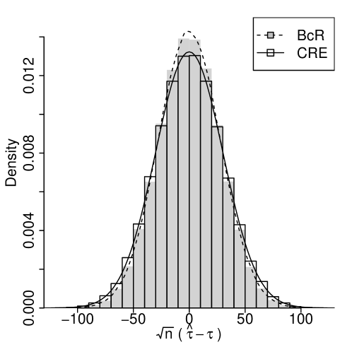
(a) Remittance

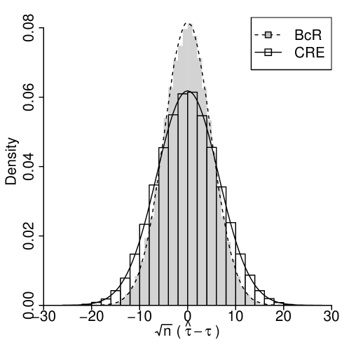
(b) Expenditure

Figure 2: Histograms and asymptotic densities of the difference-in-means estimator under the best-choice rerandomization and the CRE. The white histogram and the solid line correspond to the histogram and asymptotic density for the CRE, and the grey histogram and the dashed line correspond to the histogram and asymptotic density for the best-choice rerandomization.

Figure 2 shows the histograms of the difference-in-means estimator under the best-choice rerandomization and the CRE, based on $10^{5}$ simulated assignments from both designs. Obviously, the treatment effect estimator under the best-choice rerandomization is more concentrated around the true average treatment effect, and the improvement for the expenditure outcome is notably larger. The reason is that the pre-treatment covariates have stronger association with the potential expenditures. Specifically, both the baseline expenditure and household size have considerable associations with the potential expenditures, and the corresponding $R^{2}$ defined in (5) for measuring the strength of association between covariates and potential outcomes is $0.45$. However, for the remittance outcome, only the baseline remittance has a substantial predictive power for the potential remittances, and the corresponding $R^{2}$ is $0.15$. Nevertheless, it is worth mentioning that rerandomization can improve the precision of treatment effect estimation for multiple outcomes at the same time. In other words, the same rerandomization can benefit multiple outcome analyses.

We then consider the performance of the proposed confidence confidence intervals. For the remittance analysis, averaging over $10^{5}$ simulated assignments, the coverage probabilities of our $95\%$ confidence interval for the best-choice rerandomization and Neyman (1923)’s one for the CRE are both about $0.949$. Analogously, for the expenditure analysis, the coverage probabilities of ours and Neyman’s confidence intervals are, respectively, $0.947$ and $0.948$. All of the coverage probabilities are close to the nominal level. This is coherent with our theory since the treatment effects are constant across all units in our simulation, under which these confidence intervals will be asymptotically exact. Moreover, our confidence intervals under the best-choice rerandomization is considerably shorter than Neyman’s one under the CRE, which demonstrates the gain in inference efficiency from rerandomization. In particular, the percentage reduction in average length of confidence intervals under the best-choice rerandomization, compared to that under the CRE, is $7.3\%$ for the the remittance analysis and $24.1\%$ for the expenditure analysis. These essentially lead to $16.3\%$ and $73.8\%$ increase in effective sample size, respectively.

Discussion

We studied the large-sample analysis for the best-choice rerandomization using the Mahalanobis distance and its optimality, allowing sample-size-dependent number of covariates and number of tried complete randomizations. We showed that (i) rerandomization can outperform usual complete randomization in terms of both estimation precision and length of confidence intervals, (ii) it should incorporate appropriate number of pretreatment covariates that are relevant for the potential outcomes, and (iii) the number of tried complete randomizations should be large but not overly large, increasing at most by a polynomial order of the sample size.

In this paper we focus mainly on the best-choice rerandomization based on the completely randomized experiments and using the Mahalanobis distance measure. Like the existing literature on the first type of rerandomization, it will be interesting to further extend it to other covariate imbalance measure (e.g., Branson and Shao 2021; Zhang et al. 2021; Zhao and Ding 2021; Liu et al. 2023) and other randomized experiments (e.g., Branson et al. 2016; Li et al. 2020; Johansson and Schultzberg 2022; Wang et al. 2021). We leave these for future study.

Supplementary Material

Practical guidance for designing the best-choice rerandomization

In this section, we present the details for Section 4.3 regarding the practical guidance for designing the best-choice rerandomization with a given finite set of experimental units. In general, the asymptotic gain from the best-choice rerandomization increases with $T$, but the additional gain from increasing $T$ typically decreases with $T$; see, e.g., Figure A1 below. Thus, we suggest using large but not overly large $T$, say, $T=1000$. In addition, we should choose moderate number of covariates $K$, trying to make their association with potential outcomes, measured by $R^{2}$, large. We should avoid excessively large value of $K$ that provides little increment on $R^{2}$ but substantially increase the variance $v_{K,T}$ of the constrained Gaussian random variable, which will ultimately diminish the gain from rerandomization, as implied by Corollary 2. Below we provide some useful practical guidance when designing a best-choice rerandomization.

First, we can check the efficiency improvement from a specific choice of $T$ for the best-choice rerandomization. From Corollary 2 and Theorem 4, the difference between a best-choice rerandomization with a particular choice of $T$ and the optimal one is $R^{2}-(1-v_{K,T})R^{2}=v_{K,T}R^{2}\leq v_{K,T}$. Thus, the variance of the constrained Gaussian random variable, $v_{K,T}$, actually gives an upper bound on the gap between a particular rerandomization design and the optimal one. In practice, we can choose $T$ such that this gap is reasonably small, say, below $0.05$ or $0.1$. Figure A1 shows the value of $v_{K,T}$ when $K$ ranges from $1$ to $40$ and $T$ ranges from $10$ to $10^{4}$. Obviously, the value of $v_{K,T}$ increases with $K$ and decreases with $T$. Below we investigate the choice of $T$ such that $v_{K,T}$ is bounded by $0.1$. When $K=1$, $v_{K,T}$ is about $2.5\%$ when $T=10$; when $K=5$, $v_{K,T}$ is about $0.1$ when $T=100$; when $K=10$, $v_{K,T}$ is about $0.1$ when $T$ is about $3000$; when $K\geq 20$, we need $T$ to be greater than $10^{4}$ in order to make $v_{K,T}$ bounded by $0.1$. These indicate that in practice we should not include too many covariates into rerandomization, since they would require much larger $T$ in order to make the best-choice rerandomization close to the optimal one; intuitively, this will also lead to higher computation cost and less accurate asymptotic approximation.

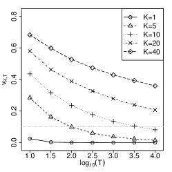
Figure A1: The variance $v_{K,T}$ of the constrained Gaussian random variable for various $(K,T)$.

Second, we can evaluate the trade-off between the potential gain and the worst-case loss from the best-choice rerandomization, as suggested in Wang and Li [2022]. As demonstrated before, the best-choice rerandomization can asymptotically improve the precision of the difference-in-means estimator compared to the CRE. With finite sample size, the CRE is actually the minimax optimal in terms of the mean squared error of the difference-in-means estimator, when we considering the worst-case scenario over all possible configurations of the potential outcomes [see, e.g., Wang and Li, 2022, Proposition A1]. Note that this does not contradict with our asymptotic theory, since, in the worst case with $R^{2}=0$, the asymptotic distribution of the difference-in-means estimator under the best-choice rerandomization is the same as that under the CRE. These two observations then provide a quantitative way to characterize the trade-off when designing rerandomization. Intuitively, we can use Corollary 2 to characterize the potential gain, and the worst-case mean squared error, which can be estimated by the Monte Carlo method, to characterize the worst-case loss. We can then consider these trade-offs when comparing multiple rerandomization designs. We will discuss this in more detail in Section A2.

Simulation using the student achievement and retention project

In this section, we provide the details for Section 6.1. The Student Achievement and Retention (STAR) project aims to evaluate the effect of academic services and incentives for college students. We focus on the comparison between two treatment arms, where the treated students would receive an array of support services and cash awards for meeting a target GPA and the control students received only standard support services.

We preprocess the data in the same way as Wang and Li [2022]. We remove units with missing covariates, resulting in $n_{1}=118$ treated units and $n_{0}=856$ control units, and generate $200$ pretreatment covariates for these $n=974$ units. Specifically, the first $5$ covariates are from the STAR project, including high-school GPA, age, gender and indicators for whether lives at home and whether rarely puts off studying for tests, and the remaining $195$ covariates are generated independently from the $t$ distribution with degrees of freedom $2$. We use the first year GPA from the STAR project as the outcome and let both treatment and control potential outcomes be the same as the observed ones, so that we are able to evaluate the repeated-sampling properties of various designs. Once generated, the potential outcomes and covariates will be kept fixed during the simulation, mimicking the finite population inference. Table A1 shows the empirical bias, root mean squared error and coverage probabilities based on $10^{5}$ draws from the best-choice rerandomization using the first $K$ covariates and $T$ number of tried complete randomizations, for various choices of $(K,T)$. Surprisingly, we find that the best-choice rerandomization performs relatively well even when $K$ and $T$ are large, although the confidence intervals become slightly under-covered when $K$ is large. These show the robustness of the best-choice rerandomization design in the presence of high-dimensional covariates and large number of tried complete randomizations. Note that these do not contradict with the intuition from our theory, which implies the potential danger of large $K$ and $T$. As shown below, for some potential outcome configurations, the performance of rerandomization can deteriorate significantly as $K$ and $T$ increase.

Table A1: Simulations under the best-choice rerandomization with various choices of $(K,T)$. The first two columns show the values of $K$ and $T$. The 2nd-7th columns show the bias, root mean squared error, and coverage probabilities of confidence intervals using various finite-sample adjustments as discussed in Section 5 when the potential outcomes are imputed based on the observed ones. The 8th-13th columns show analogous quantities when the potential outcomes are quantile transformations of the average propensity scores across all the considered rerandomization designs.

$K$	$T$	Bias	RMSE	HC0	HC1	HC2	HC3	Bias	RMSE	HC0	HC1	HC2	HC3
$5$	$10$	$0.012$	$0.889$	$0.950$	$0.955$	$0.955$	$0.957$	$-0.022$	$0.965$	$0.958$	$0.958$	$0.958$	$0.960$
$5$	$100$	$0.003$	$0.910$	$0.939$	$0.943$	$0.944$	$0.952$	$0.033$	$0.977$	$0.950$	$0.952$	$0.952$	$0.952$
$5$	$1000$	$-0.023$	$0.874$	$0.950$	$0.955$	$0.955$	$0.961$	$0.027$	$1.022$	$0.941$	$0.942$	$0.942$	$0.942$
$5$	$10000$	$0.022$	$0.918$	$0.937$	$0.943$	$0.944$	$0.948$	$0.000$	$0.966$	$0.960$	$0.963$	$0.963$	$0.964$
$10$	$10$	$0.026$	$0.977$	$0.929$	$0.934$	$0.934$	$0.941$	$0.163$	$1.037$	$0.925$	$0.931$	$0.931$	$0.933$
$10$	$100$	$0.007$	$0.891$	$0.946$	$0.950$	$0.950$	$0.955$	$0.240$	$1.021$	$0.925$	$0.940$	$0.940$	$0.946$
$10$	$1000$	$-0.004$	$0.890$	$0.938$	$0.947$	$0.947$	$0.955$	$0.308$	$0.991$	$0.931$	$0.941$	$0.941$	$0.944$
$10$	$10000$	$-0.051$	$0.907$	$0.931$	$0.943$	$0.943$	$0.952$	$0.289$	$1.035$	$0.917$	$0.930$	$0.932$	$0.936$
$50$	$10$	$0.054$	$1.008$	$0.932$	$0.945$	$0.946$	$0.952$	$0.440$	$1.063$	$0.893$	$0.909$	$0.912$	$0.914$
$50$	$100$	$0.006$	$0.983$	$0.921$	$0.940$	$0.941$	$0.947$	$0.704$	$1.183$	$0.837$	$0.869$	$0.870$	$0.874$
$50$	$1000$	$-0.039$	$0.890$	$0.943$	$0.961$	$0.962$	$0.969$	$0.911$	$1.334$	$0.762$	$0.812$	$0.815$	$0.822$
$50$	$10000$	$0.008$	$0.894$	$0.936$	$0.963$	$0.964$	$0.970$	$1.104$	$1.451$	$0.685$	$0.752$	$0.757$	$0.770$
$100$	$10$	$0.014$	$0.953$	$0.921$	$0.946$	$0.946$	$0.950$	$0.535$	$1.072$	$0.870$	$0.898$	$0.897$	$0.908$
$100$	$100$	$0.063$	$0.944$	$0.918$	$0.951$	$0.951$	$0.954$	$0.978$	$1.342$	$0.722$	$0.784$	$0.789$	$0.806$
$100$	$1000$	$-0.011$	$0.965$	$0.892$	$0.942$	$0.944$	$0.952$	$1.126$	$1.488$	$0.614$	$0.704$	$0.710$	$0.728$
$100$	$10000$	$0.060$	$0.948$	$0.894$	$0.952$	$0.952$	$0.962$	$1.361$	$1.632$	$0.530$	$0.619$	$0.626$	$0.652$
$200$	$10$	$0.048$	$0.960$	$0.901$	$0.902$	$0.902$	$0.904$	$0.630$	$1.184$	$0.782$	$0.783$	$0.783$	$0.803$
$200$	$100$	$0.021$	$0.973$	$0.889$	$0.889$	$0.889$	$0.896$	$0.937$	$1.320$	$0.714$	$0.720$	$0.721$	$0.749$
$200$	$1000$	$0.022$	$0.936$	$0.884$	$0.884$	$0.884$	$0.890$	$1.188$	$1.515$	$0.608$	$0.615$	$0.621$	$0.655$
$200$	$10000$	$-0.021$	$0.978$	$0.871$	$0.877$	$0.877$	$0.888$	$1.384$	$1.677$	$0.489$	$0.496$	$0.502$	$0.541$

We now consider another way of generating potential outcomes. We first use Monte Carlo method to estimate the propensity scores of each unit averaging over the best-choice rerandomization designs under investigation, and then take a Gaussian quantile transformation to generate both potential outcomes, where the treatment and control potential outcomes for each unit are the same. With this potential outcome configuration, Table A1 shows analogously the empirical bias, root mean squared error and coverage probabilities under the best-choice rerandomization designs with various choices of $(K,T)$. Obviously, as $K$ and $T$ increases, both the bias and mean squared error tend to be larger, and the coverage probabilities become much smaller than the nominal level. Thus, the performance of the best-choice rerandomization can be sensitive to the potential outcome configuration when $K$ and $T$ are large. Below we present two practical ways to tackle this issue.

First, we can check the worst-case behavior of the best-choice rerandomization using the formula derived in Wang and Li [2022, Proposition A1]. As shown in Table A2, both the worst-case bias and root mean squared error increase notably as $K$ and $T$ increases. It is worth mentioning that there is considerable Monte Carlo error even when we use $10^{5}$ simulated assignments to estimate the worst-case root mean squared error; for example, the estimated worst-case bias and root mean squared error for the CRE is about $0.1$ and $1.1$, whose true values are known to be $0$ and $1$. We can increase the number of simulated assignments to make the Monte Carlo estimation more accurate, but the trend in Table A2 already illustrates the potential drawback of large $K$ and $T$. As discussed in Section A1, in practice, we can also combine this with the potential gain that rerandomization can bring as shown in Corollary 2 to guide our design of rerandomization. For example, similar to Wang and Li [2022], we can use the geometric mean of the worst-case mean squared error and the ideal-case mean squared error implied by the asymptotic theory as a measure for comparing different best-choice rerandomization designs. Note that the asymptotic mean squared error (or equivalently the asymptotic variance since $\hat{\tau}$ is asymptotically unbiased under rerandomization) depends on the association between potential outcomes and covariates, measured by $R^{2}$ in (5), which needs to be determined by domain knowledge or prior studies.

Table A2: Worst-case bias (top half) and root mean squared error (bottom half) of the best-choice rerandomization with various choices of $(K,T)$. The $2$nd-$5$th columns use the original covariates for rerandomization, and the $6$th-$9$th columns use the trimmed covariates.

		Original covariates					Trimmed covariates
		$10$	$100$	$1000$	$10000$		$10$	$100$	$1000$	$10000$
$5$		$0.117$	$0.126$	$0.134$	$0.131$		$0.109$	$0.113$	$0.115$	$0.112$
$10$		$0.512$	$0.682$	$0.793$	$0.850$		$0.137$	$0.162$	$0.166$	$0.174$
$50$		$0.823$	$1.204$	$1.444$	$1.620$		$0.160$	$0.214$	$0.254$	$0.277$
$100$		$0.853$	$1.305$	$1.600$	$1.822$		$0.161$	$0.213$	$0.268$	$0.309$
$200$		$0.798$	$1.244$	$1.566$	$1.819$		$0.167$	$0.236$	$0.288$	$0.331$
$5$		$1.099$	$1.101$	$1.099$	$1.100$		$1.100$	$1.100$	$1.102$	$1.099$
$10$		$1.102$	$1.140$	$1.193$	$1.227$		$1.100$	$1.102$	$1.102$	$1.103$
$50$		$1.157$	$1.411$	$1.615$	$1.773$		$1.104$	$1.108$	$1.112$	$1.115$
$100$		$1.186$	$1.504$	$1.754$	$1.955$		$1.107$	$1.113$	$1.119$	$1.122$
$200$		$1.185$	$1.483$	$1.753$	$1.974$		$1.109$	$1.121$	$1.128$	$1.133$

Second, we can perform trimming to effectively improve the worst-case performance of the best-choice rerandomization, a strategy that has also been used by Lei and Ding [2020] and Wang and Li [2022]. Note that under our randomization-based inference without any model assumptions, we have the flexibility to conduct arbitrary pre-processing of the covariates. The intuition of trimming is similar to that discussed in Morgan and Rubin [2012] with small sample size. When a unit has extreme covariates, it is more likely to be allocated to the group of larger size under rerandomization, which can help balance the covariates between the two groups. The extremeness of covariates also appears on the Berry-Esseen bound in (7), which depends crucially on the leverages scores of the covariate matrix [Wang and Li, 2022]. Trimming can help us mitigate the extreme covariates, thereby improving the robustness of the best-choice rerandomization. For example, we trim each covariate at its $2.5\%$ and $97.5\%$ quantiles, and analogously calculate the worst-case performance as shown in Table A2. Obviously, the performance of the best-choice rerandomization enhances after trimming. Indeed, the propensity scores of units under these rerandomization designs with the original covariates range from $0.00032$ to $0.146$, while that with trimmed covariates range from $0.109$ to $0.131$, which are much more stable and concentrate around $n_{1}/n=0.121$.

Remark A4.

We finally comment on the comparison between the best-choice rerandomization and rerandomization based on a prespecified imbalance threshold. Comparing Table A2 and Table A1 in Wang and Li [2022], given the same number of covariates, the worst-case mean squared errors under the best-choice rerandomization trying $T$ complete randomizations are comparable to the first-type rerandomization with acceptance probability $1/T$. This echos the intuitive and theoretical comparisons in Remarks 1–3. However, the best-choice rerandomization can be more stable in practice, because it can always produce “acceptable” randomizations. Besides, its implementation is intuitive, convenient, and has already been used frequently in practice.

Proof for the asymptotic distribution of the difference-in-means estimator under the best-choice rerandomization

To prove Theorem 1, we need the following three lemmas.

Lemma A1.

Let $(\hat{\tau},\hat{\boldsymbol{\tau}}_{\boldsymbol{x}}^{\top})^{\top}$ be the difference-in-means of outcomes and covariates under the CRE, and $(\tilde{\tau},\tilde{\boldsymbol{\tau}}_{\boldsymbol{x}}^{\top})^{\top}$ be a Gaussian random vector with mean zero and covariance matrix $\boldsymbol{V}$ in (4). Let $M=\hat{\boldsymbol{\tau}}_{\boldsymbol{x}}^{\top}\boldsymbol{V}_{\boldsymbol{xx}}^{-1}\hat{\boldsymbol{\tau}}_{\boldsymbol{x}}$ denote the Mahalanobis distance as in (2), and define analogously $M=\tilde{\boldsymbol{\tau}}_{\boldsymbol{x}}^{\top}\boldsymbol{V}_{\boldsymbol{xx}}^{-1}\tilde{\boldsymbol{\tau}}_{\boldsymbol{x}}$. Then for any $c_{1},c_{2}\in\mathbb{R}$, with $\Delta_{n}$ defined as in (6),

$$\sup_{c_{1},c_{2}\in\mathbb{R}}\big{|}\mathbb{P}(\hat{\tau}-\tau\leq c_{1},M\leq c_{2})-\mathbb{P}(\tilde{\tau}\leq c_{1},\tilde{M}\leq c_{2})\big{|} \leq\Delta_{n},$$

$$\sup_{c_{1},c_{2}\in\mathbb{R}}\big{|}\mathbb{P}(\hat{\tau}-\tau\leq c_{1},M<c_{2})-\mathbb{P}(\tilde{\tau}\leq c_{1},\tilde{M}<c_{2})\big{|} \leq\Delta_{n},$$

$$\sup_{c\in\mathbb{R}}\big{|}\mathbb{P}(M\geq c)-\mathbb{P}(\tilde{M}\geq c)\big{|} \leq\Delta_{n},$$

$$\sup_{c\in\mathbb{R}}\big{|}\mathbb{P}(M>c)-\mathbb{P}(\tilde{M}>c)\big{|} \leq\Delta_{n}.$$

Proof of Lemma A1.

Lemma A1 follows directly from the definition of $\Delta_{n}$ and the fact that the sets $\{\boldsymbol{w}:\boldsymbol{w}^{\top}\boldsymbol{V}_{\boldsymbol{xx}}^{-1}\boldsymbol{w}\leq c\}$ and $\{\boldsymbol{w}:\boldsymbol{w}^{\top}\boldsymbol{V}_{\boldsymbol{xx}}^{-1}\boldsymbol{w}<c\}$ are convex for any $c\in\mathbb{R}$. ∎

Lemma A2.

Under the same setting as Lemma A1, let $(A_{1},B_{1}),\ldots,(A_{J},B_{J})$ be any random vectors that are independent of $(\hat{\tau},\hat{\boldsymbol{\tau}}_{\boldsymbol{x}}^{\top})^{\top}$ and $(\tilde{\tau},\tilde{\boldsymbol{\tau}}_{\boldsymbol{x}}^{\top})^{\top}$; Define

$$(A_{0},B_{0})\equiv(\hat{\tau}-\tau,M),\quad(\tilde{A}_{0},\tilde{B}_{0})\equiv(\tilde{\tau},\tilde{M}),\quad(\tilde{A}_{j},\tilde{B}_{j})\equiv(A_{j},B_{j})\text{ for }1\leq j\leq J.$$

Then for any $c\in\mathbb{R}$,

$$\mathbb{P}\left(\bigcup_{j=0}^{J}\Big{\{}A_{j}\leq c,B_{j}\leq\min_{k\neq j}B_{k}\Big{\}}\right)-\mathbb{P}\left(\bigcup_{j=0}^{J}\Big{\{}\tilde{A}_{j}\leq c,\tilde{B}_{j}\leq\min_{k\neq j}\tilde{B}_{k}\Big{\}}\right)\leq 2\Delta_{n}.$$

Proof of Lemma A2.

By the law of iterated expectation,

$$\quad\ \mathbb{P}\left(\bigcup_{j=0}^{J}\Big{\{}A_{j}\leq c,B_{j}\leq\min_{k\neq j}B_{k}\Big{\}}\right)=\mathbb{E}\left[\mathbb{P}\left(\bigcup_{j=0}^{T}\Big{\{}A_{j}\leq c,B_{j}\leq\min_{k\neq j}B_{k}\Big{\}}\mid A_{1:J},B_{1:J}\right)\right]$$

$$=\mathbb{E}\left[\mathbb{P}\left(\Big{\{}A_{0}\leq c,B_{0}\leq\min_{k>0}B_{k}\Big{\}}\bigcup\Big{\{}\mathcal{E}_{0}\cap\{B_{0}\geq\min_{k>0}B_{k}\}\Big{\}}\mid A_{1:J},B_{1:J}\right)\right],$$ (A1)

where

$$\mathcal{E}_{0}\equiv\bigcup_{j=1}^{J}\Big{\{}A_{j}\leq c,B_{j}\leq\min_{k\neq 0,j}B_{k}\Big{\}}$$

is an event that becomes deterministic once conditioning on $A_{1:J}\equiv(A_{1},\ldots,A_{J})$ and $B_{1:J}\equiv(B_{1},\ldots,B_{J})$. By the union bound,

$$\quad\ \mathbb{P}\left(\bigcup_{j=0}^{J}\Big{\{}A_{j}\leq c,B_{j}\leq\min_{k\neq j}B_{k}\Big{\}}\right)$$

$$\leq\mathbb{E}\left[\mathbb{P}\Big{(}A_{0}\leq c,B_{0}\leq\min_{k>0}B_{k}\mid A_{1:J},B_{1:J}\Big{)}+\mathbb{P}\Big{(}B_{0}\geq\min_{k>0}B_{k}\mid A_{1:J},B_{1:J}\Big{)}\mathbbm{1}(\mathcal{E}_{0})\right].$$

Note that both $(A_{0},B_{0})$ and $(\tilde{A}_{0},\tilde{B}_{0})$ are independent of $(A_{1:J},B_{1:J})$. From Lemma A1, we then have

$$\quad\ \mathbb{P}\left(\bigcup_{j=0}^{J}\Big{\{}A_{j}\leq c,B_{j}\leq\min_{k\neq j}B_{k}\Big{\}}\right)$$

$$\leq\mathbb{E}\left[\mathbb{P}\Big{(}\tilde{A}_{0}\leq c,\tilde{B}_{0}\leq\min_{k>0}B_{k}\mid A_{1:J},B_{1:J}\Big{)}+\mathbb{P}\Big{(}\tilde{B}_{0}\geq\min_{k>0}B_{k}\mid A_{1:J},B_{1:J}\Big{)}\mathbbm{1}(\mathcal{E}_{0})\right]+2\Delta_{n}$$

$$=\mathbb{E}\left[\mathbb{P}\left(\Big{\{}\tilde{A}_{0}\leq c,\tilde{B}_{0}\leq\min_{k>0}B_{k}\Big{\}}\bigcup\Big{\{}\mathcal{E}_{0}\cap\{\tilde{B}_{0}\geq\min_{k>0}B_{k}\}\Big{\}}\mid A_{1:J},B_{1:J}\right)\right]+2\Delta_{n}$$

$$=\mathbb{P}\left(\bigcup_{j=0}^{J}\Big{\{}\tilde{A}_{j}\leq c,\tilde{B}_{j}\leq\min_{k\neq j}\tilde{B}_{k}\Big{\}}\right)+2\Delta_{n},$$

where the second last equality holds because $\tilde{B}_{0}$ is a continuous random variable and consequently the measure of the intersection of the two events there is zero, and the last equality holds by the same logic as (A3). Therefore, Lemma A2 holds. ∎

Lemma A3.

Under the same setting as Lemma A2, for any $c\in\mathbb{R}$,

$$\mathbb{P}\left(\bigcup_{j=0}^{J}\Big{\{}A_{j}\leq c,B_{j}<\min_{k\neq j}B_{k}\Big{\}}\right)-\mathbb{P}\left(\bigcup_{j=0}^{J}\Big{\{}\tilde{A}_{j}\leq c,\tilde{B}_{j}<\min_{k\neq j}\tilde{B}_{k}\Big{\}}\right)\geq-2\Delta_{n}.$$

Proof of Lemma A3.

By the law of iterated expectation,

$$\quad\ \mathbb{P}\left(\bigcup_{j=0}^{J}\Big{\{}A_{j}\leq c,B_{j}<\min_{k\neq j}B_{k}\Big{\}}\right)$$

$$=\mathbb{E}\left[\mathbb{P}\left(\Big{\{}A_{0}\leq c,B_{0}<\min_{k>0}B_{k}\Big{\}}\bigcup\Big{\{}\mathcal{E}_{0}^{\prime}\cap\{B_{0}>\min_{k>0}B_{k}\}\Big{\}}\mid A_{1:J},B_{1:J}\right)\right]$$

$$=\mathbb{E}\left[\mathbb{P}\left(A_{0}\leq c,B_{0}<\min_{k>0}B_{k}\mid A_{1:J},B_{1:J}\right)\right]+\mathbb{E}\left[\mathbbm{1}(\mathcal{E}_{0}^{\prime})\mathbb{P}\left(B_{0}>\min_{k>0}B_{k}\mid A_{1:J},B_{1:J}\right)\right],$$ (A2)

where

$$\mathcal{E}_{0}^{\prime}\equiv\bigcup_{j=1}^{J}\Big{\{}A_{j}\leq c,B_{j}<\min_{k\neq 0,j}B_{k}\Big{\}}$$

is an event that becomes deterministic once conditioning on $A_{1:J}\equiv(A_{1},\ldots,A_{J})$ and $B_{1:J}\equiv(B_{1},\ldots,B_{J})$, and the last equality holds because the two events there are disjoint. Note that both $(A_{0},B_{0})$ and $(\tilde{A}_{0},\tilde{B}_{0})$ are independent of $(A_{1:J},B_{1:J})$. From Lemma A1, we then have

$$\quad\ \mathbb{P}\left(\bigcup_{j=0}^{J}\Big{\{}A_{j}\leq c,B_{j}<\min_{k\neq j}B_{k}\Big{\}}\right)$$

$$\geq\mathbb{E}\left[\mathbb{P}\left(\tilde{A}_{0}\leq c,\tilde{B}_{0}<\min_{k>0}B_{k}\mid A_{1:J},B_{1:J}\right)\right]+\mathbb{E}\left[\mathbbm{1}(\mathcal{E}_{0}^{\prime})\mathbb{P}\left(\tilde{B}_{0}>\min_{k>0}B_{k}\mid A_{1:J},B_{1:J}\right)\right]-2\Delta_{n}$$

$$=\mathbb{P}\left(\bigcup_{j=0}^{J}\Big{\{}\tilde{A}_{j}\leq c,\tilde{B}_{j}<\min_{k\neq j}\tilde{B}_{k}\Big{\}}\right)-2\Delta_{n},$$

where the last equality holds by the same logic as (A3). ∎

Proof of Theorem 1.

Recall the definition of $\boldsymbol{Z}_{[t]}$’s, $M_{[t]}$’s and $\hat{\tau}_{(1)}$ in Section 3. Define further $\hat{\tau}_{[t]}$ as the difference-in-means estimator under the treatment assignment $\boldsymbol{Z}_{[t]}$, for $1\leq t\leq T$. By the construction of the best-choice rerandomization, for any $c\in\mathbb{R}$,

$$\mathbb{P}\left(\bigcup\limits_{t=1}^{T}\big{\{}\hat{\tau}_{[t]}-\tau\leq c,M_{[t]}<\min_{j\neq t}M_{[j]}\big{\}}\right)\leq\mathbb{P}(\hat{\tau}_{(1)}-\tau\leq c)\leq\mathbb{P}\left(\bigcup\limits_{t=1}^{T}\big{\{}\hat{\tau}_{[t]}-\tau\leq c,M_{[t]}\leq\min_{j\neq t}M_{[j]}\big{\}}\right),$$ (A3)

where the inequality in (A3) comes mainly from the fact that there may be multiple treatment assignments achieving the minimum covariate imbalance. Recall also the definition of $\tilde{\tau}_{[t]}$’s and $\tilde{M}_{[t]}$’s in Section 3.2. Furthermore, without loss of generality, we assume that $\tilde{\tau}_{[t]}$’s and $\tilde{M}_{[t]}$’s are independent of $\hat{\tau}_{[t]}$’s and $M_{[t]}$’s. Obviously, for all $t$, $\tilde{M}_{[t]}$ follows the chi-squared distribution with degrees of freedom $K$.

First, we consider the upper bound of $\mathbb{P}(\hat{\tau}_{(1)}-\tau\leq c)$. For $0\leq j\leq T$, define

$$(A_{t}^{(j)},B_{t}^{(j)}) =\begin{cases}(\hat{\tau}_{[t]}-\tau,M_{[t]}),&\textup{if }t>j,\\ (\tilde{\tau}_{[t]},M_{[t]}),&\textup{if }t\leq j,\end{cases}\quad(1\leq t\leq T).$$

Obviously, $\{(A_{t}^{(j)},B_{t}^{(j)}):1\leq t\leq T\}$ and $\{(A_{t}^{(j+1)},B_{t}^{(j+1)}):1\leq t\leq T\}$ differ only in the $(j+1)$th element, for $0\leq j\leq T-1$. This allows us to apply Lemma A2 to get that, for any $0\leq j\leq T-1$,

$$\mathbb{P}\left(\bigcup\limits_{t=1}^{T}\big{\{}A_{t}^{(j)}\leq c,B_{t}^{(j)}\leq\min_{j\neq t}B_{j}^{(j)}\big{\}}\right)\leq\mathbb{P}\left(\bigcup\limits_{t=1}^{T}\big{\{}A_{t}^{(j+1)}\leq c,B_{t}^{(j+1)}\leq\min_{j\neq t}B_{j}^{(j+1)}\big{\}}\right)+2\Delta_{n},$$

where in the above inequality we take $(A_{j+1}^{(j)},B_{j+1}^{(j)})$ and $(A_{j+1}^{(j+1)},B_{j+1}^{(j+1)})$ as $(A_{0},B_{0})$ and $(\tilde{A}_{0},\tilde{B}_{0})$; and take $\{(A_{t}^{(j)},B_{t}^{(j)}),0\leq t\leq T\;\&\;t\neq j+1\}$ and $\{(A_{t}^{(j+1)},B_{t}^{(j+1)}),0\leq t\leq T\;\&\;t\neq j+1\}$ as $\{(A_{j},B_{j}),1\leq j\leq J\}$ and $\{(\tilde{A}_{j},\tilde{B}_{j}),1\leq j\leq J\}$. Armed with the above inequality, we have

$$\mathbb{P}(\hat{\tau}_{(1)}-\tau\leq c) \leq\mathbb{P}\left(\bigcup\limits_{t=1}^{T}\big{\{}\hat{\tau}_{[t]}-\tau\leq c,M_{[t]}\leq\min_{j\neq t}M_{[j]}\big{\}}\right)=\mathbb{P}\left(\bigcup\limits_{t=1}^{T}\big{\{}A_{t}^{(0)}\leq c,B_{t}^{(0)}\leq\min_{j\neq t}B_{j}^{(0)}\big{\}}\right)$$

$$\leq\mathbb{P}\left(\bigcup\limits_{t=1}^{T}\big{\{}A_{t}^{(1)}\leq c,B_{t}^{(1)}\leq\min_{j\neq t}B_{j}^{(1)}\big{\}}\right)+2\Delta_{n}$$

$$\leq\mathbb{P}\left(\bigcup\limits_{t=1}^{T}\big{\{}A_{t}^{(2)}\leq c,B_{t}^{(2)}\leq\min_{j\neq t}B_{j}^{(2)}\big{\}}\right)+2\times 2\Delta_{n}$$

$$\leq\ldots\leq\mathbb{P}\left(\bigcup\limits_{t=1}^{T}\big{\{}A_{t}^{(T)}\leq c,B_{t}^{(T)}\leq\min_{j\neq t}B_{j}^{(T)}\big{\}}\right)+T\times 2\Delta_{n}$$

$$=\mathbb{P}\left(\bigcup\limits_{t=1}^{T}\big{\{}\tilde{\tau}_{[t]}\leq c,\tilde{M}_{[t]}\leq\min_{j\neq t}\tilde{M}_{[j]}\big{\}}\right)+2T\Delta_{n}.$$

Second, we consider the lower bound of $\mathbb{P}(\hat{\tau}_{(1)}-\tau\leq c)$. By the same logic as the proof of the upper bound and applying Lemma A3, we have

$$\mathbb{P}(\hat{\tau}_{(1)}-\tau\leq c)\geq\mathbb{P}\left(\bigcup\limits_{t=1}^{T}\big{\{}\tilde{\tau}_{[t]}\leq c,\tilde{M}_{[t]}<\min_{j\neq t}\tilde{M}_{[j]}\big{\}}\right)-2T\Delta_{n}.$$

Third, we prove that, for any $c\in\mathbb{R}$,

$$\mathbb{P}\left(\bigcup\limits_{t=1}^{T}\big{\{}\tilde{\tau}_{[t]}\leq c,\tilde{M}_{[t]}<\min_{j\neq t}\tilde{M}_{[j]}\big{\}}\right)=\mathbb{P}(\tilde{\tau}_{(1)}\leq c)=\mathbb{P}\left(\bigcup\limits_{t=1}^{T}\big{\{}\tilde{\tau}_{[t]}\leq c,\tilde{M}_{[t]}\leq\min_{j\neq t}\tilde{M}_{[j]}\big{\}}\right).$$ (A4)

By the same logic as (A3), the left-hand side of (A4) is bounded from above by $\mathbb{P}(\tilde{\tau}_{(1)}\leq c)$, which is further bounded from above by the right-hand side of (A4). Furthermore, the right-hand side of (A4) is also bounded from above by the left-hand side:

$$\quad\ \mathbb{P}\left(\bigcup\limits_{t=1}^{T}\big{\{}\tilde{\tau}_{[t]}\leq c,\tilde{M}_{[t]}\leq\min_{j\neq t}\tilde{M}_{[j]}\big{\}}\right)-\mathbb{P}\left(\bigcup\limits_{t=1}^{T}\big{\{}\tilde{\tau}_{[t]}\leq c,\tilde{M}_{[t]}<\min_{j\neq t}\tilde{M}_{[j]}\big{\}}\right)$$

$$\leq\mathbb{P}\left(\bigcup\limits_{t=1}^{T}\bigcup\limits_{j\neq t}\big{\{}\tilde{M}_{[t]}=\tilde{M}_{[j]}\big{\}}\right)=0,$$

where the last equality holds because $\tilde{M}_{[j]}$’s are mutually independent continuous random variables. These facts then imply that (A4) must hold.

From the above, we then have that $|\mathbb{P}(\hat{\tau}_{(1)}-\tau\leq c)-\mathbb{P}(\tilde{\tau}_{(1)}\leq c)|\leq 2T\Delta_{n}$ for any $c\in\mathbb{R}$. Equivalently, the inequality in (8) holds. If Conditions 1 and 2 hold, then $T\Delta_{n}=o(1)$, and consequently the supremum in (8) converges to zero as $n\rightarrow\infty$. Therefore, Theorem 1 holds. ∎

To prove Theorem 2, we need the following lemma.

Lemma A4.

Let $\boldsymbol{D}_{1},\ldots,\boldsymbol{D}_{T}\in\mathbb{R}^{K}$ be $T$ mutually independent $K$-dimensional standard Gaussian random vectors. Then, for any constant unit vector $\boldsymbol{c}\in\mathbb{R}^{K}$,

$$\boldsymbol{c}^{\top}\boldsymbol{D}_{1}\mid\|\boldsymbol{D}_{1}\|_{2}^{2}\leq\min_{1\leq j\leq T}\|\boldsymbol{D}_{j}\|_{2}^{2}\ \sim\ D_{11}\mid\|\boldsymbol{D}_{1}\|_{2}^{2}\leq\min_{1\leq j\leq T}\|\boldsymbol{D}_{j}\|_{2}^{2},$$

where $D_{11}$ is the first coordinate of $\boldsymbol{D}_{1}$.

Proof of Lemma A4.

For any given unit vector $\boldsymbol{c}\in\mathbb{R}^{K}$, we can always construct an orthogonal matrix $\boldsymbol{C}$ whose first row is $\boldsymbol{c}^{\top}$. Then $\boldsymbol{c}^{\top}\boldsymbol{D}_{1}$ will be the first coordinate of $\boldsymbol{C}\boldsymbol{D}_{1}$, and $\|\boldsymbol{C}\boldsymbol{D}_{j}\|_{2}^{2}=\|\boldsymbol{D}_{j}\|_{2}^{2}$ for all $1\leq j\leq T$. By the property of standard Gaussian distributions, $(\boldsymbol{C}\boldsymbol{D}_{1},\ldots,\boldsymbol{C}\boldsymbol{D}_{T})$ follows the same distribution as $(\boldsymbol{D}_{1},\ldots,\boldsymbol{D}_{T})$. This then implies Lemma A4. ∎

Proof of Theorem 2.

From equation (A4) in the proof of Theorem 1, for any $c\in\mathbb{R}$,

$$\mathbb{P}(\tilde{\tau}_{(1)}\leq c) =\mathbb{P}\left(\bigcup\limits_{t=1}^{T}\big{\{}\tilde{\tau}_{[t]}\leq c,\tilde{M}_{[t]}\leq\min_{j\neq t}\tilde{M}_{[j]}\big{\}}\right)=\sum_{t=1}^{T}\mathbb{P}\Big{(}\tilde{\tau}_{[t]}\leq c,\tilde{M}_{[t]}\leq\min_{j\neq t}\tilde{M}_{[j]}\Big{)},$$

where the last equality holds because $\tilde{M}_{[t]}$’s are mutually independent continuous random variables. Because $(\tilde{\tau}_{[t]},\tilde{M}_{[t]})$’s are i.i.d.  across all $t$, and $\tilde{M}_{[t]}$’s are continuous random variables, we then have $\mathbb{P}(\tilde{M}_{[1]}\leq\min_{1\leq j\leq T}\tilde{M}_{[j]})=1/T$, and

$$\quad\ \mathbb{P}(\tilde{\tau}_{(1)}\leq c)$$

$$=T\cdot\mathbb{P}\Big{(}\tilde{\tau}_{[1]}\leq c,\tilde{M}_{[1]}\leq\min_{1\leq j\leq T}\tilde{M}_{[j]}\Big{)}=T\cdot\mathbb{P}\Big{(}\tilde{M}_{[1]}\leq\min_{1\leq j\leq T}\tilde{M}_{[j]}\Big{)}\cdot\mathbb{P}\Big{(}\tilde{\tau}_{[1]}\leq c\mid\tilde{M}_{[1]}\leq\min_{1\leq j\leq T}\tilde{M}_{[j]}\Big{)}$$

$$=\mathbb{P}\Big{(}\tilde{\tau}_{[1]}\leq c\mid\tilde{M}_{[1]}\leq\min_{1\leq j\leq T}\tilde{M}_{[j]}\Big{)}.$$

Let $\tilde{\tau}_{[1]}^{\perp}=\tilde{\tau}_{[1]}-V_{\tau\boldsymbol{x}}V_{\boldsymbol{xx}}^{-1}\tilde{\boldsymbol{\tau}}_{\boldsymbol{x}[1]}$. We can verify that $\tilde{\tau}_{[1]}^{\perp}\sim\mathcal{N}(0,V_{\tau\tau}(1-R^{2}))$ and it is independent from all the $\tilde{\boldsymbol{\tau}}_{\boldsymbol{x}[t]}$’s. Let $\varepsilon_{0}\sim\mathcal{N}(0,1)$ be a standard Gaussian random variable independent of all the $\tilde{\boldsymbol{\tau}}_{\boldsymbol{x}[t]}$’s, and $\boldsymbol{D}_{t}=V_{\boldsymbol{xx}}^{-1/2}\tilde{\boldsymbol{\tau}}_{\boldsymbol{x}[t]}$ for $1\leq t\leq T$. We then have, for any $c\in\mathbb{R}$,

$$\mathbb{P}(\tilde{\tau}_{(1)}\leq c) =\mathbb{P}\Big{(}\tilde{\tau}_{[1]}\leq c\mid\tilde{M}_{[1]}\leq\min_{1\leq j\leq T}\tilde{M}_{[j]}\Big{)}=\mathbb{P}\Big{(}\tilde{\tau}_{[1]}^{\perp}+V_{\tau\boldsymbol{x}}V_{\boldsymbol{xx}}^{-1}\tilde{\boldsymbol{\tau}}_{\boldsymbol{x}[1]}\leq c\mid\tilde{M}_{[1]}\leq\min_{1\leq j\leq T}\tilde{M}_{[j]}\Big{)}$$

$$=\mathbb{P}\Big{(}\sqrt{V_{\tau\tau}(1-R^{2})}\ \varepsilon_{0}+V_{\tau\boldsymbol{x}}V_{\boldsymbol{xx}}^{-1/2}\boldsymbol{D}_{1}\leq c\mid\|\boldsymbol{D}_{1}\|_{2}^{2}\leq\min_{1\leq j\leq T}\|\boldsymbol{D}_{j}\|_{2}^{2}\Big{)}$$

$$=\mathbb{P}\Big{(}\sqrt{V_{\tau\tau}(1-R^{2})}\ \varepsilon_{0}+\sqrt{V_{\tau\tau}R^{2}}\ \boldsymbol{h}^{\top}\boldsymbol{D}_{1}\leq c\mid\|\boldsymbol{D}_{1}\|_{2}^{2}\leq\min_{1\leq j\leq T}\|\boldsymbol{D}_{j}\|_{2}^{2}\Big{)},$$

where $\boldsymbol{h}=(V_{\tau\tau}R^{2})^{-1/2}V_{\boldsymbol{xx}}^{-1/2}V_{\boldsymbol{x}\tau}$ is a unit vector of length $1$ by the definition of $R^{2}$ in (5). From Lemma A4, this further implies that $\mathbb{P}(\tilde{\tau}_{(1)}\leq c)=\mathbb{P}(\sqrt{V_{\tau\tau}(1-R^{2})}\ \varepsilon_{0}+\sqrt{V_{\tau\tau}R^{2}}\ L_{K,T}\leq c)$ for all $c\in\mathbb{R}$. We can then immediately derive Theorem 2. ∎

Proof for the properties of the asymptotic distribution

Proof of Proposition 1 and the equivalence in (11).

We first prove Proposition 1. From Lemma A4, $L_{K,T}\sim\boldsymbol{c}^{\top}\boldsymbol{D}_{1}\mid\|\boldsymbol{D}_{1}\|_{2}^{2}\leq\min_{1\leq t\leq T}\|\boldsymbol{D}_{t}\|_{2}^{2}$ for any constant unit vector $c\in\mathbb{R}^{K}$. Moreover, from Li et al. [2018, Lemma A2], it suffices to prove that $L_{K,T}\sim\chi_{K,T}U_{K}$. For all $1\leq t\leq T$, define $\xi_{t}=\|\boldsymbol{D}_{t}\|_{2}$. By the property of the multivariate standard Gaussian distribution, $\xi_{t}^{2}$ follows chi-squared distribution with degrees of freedom $K$, $\boldsymbol{D}_{t}/\xi_{t}$ follows the uniform distribution on the $K-1$ dimensional unit sphere, and they are mutually independent. These imply that, with $D_{11}$ and $[\boldsymbol{D}_{1}/\xi_{1}]_{1}$ being the first coordinates of $\boldsymbol{D}_{1}$ and $\boldsymbol{D}_{1}/\xi_{1}$, respectively,

$$L_{K,T}\ \sim\ D_{11}\mid\|\boldsymbol{D}_{1}\|_{2}^{2}\leq\min_{1\leq t\leq T}\|\boldsymbol{D}_{j}\|_{2}^{2}\ \sim\ [\boldsymbol{D}_{t}/\xi_{t}]_{1}\xi_{1}\mid\xi_{1}^{2}\leq\min_{1\leq t\leq T}\xi_{t}^{2}\ \sim\ U_{K}\xi_{1}\mid\xi_{1}\leq\min_{1\leq t\leq T}\xi_{t}.$$ (A5)

Consequently, Proposition 1 holds.

We then prove the equivalence in (11). The fact that $\chi^{2}_{K(1)}\sim F_{K}^{-1}(\text{Beta}(1,T))$ follows from the property of order statistics. It then suffices to prove that $\xi_{1}\mid\xi_{1}\leq\min_{1\leq t\leq T}\xi_{t}\sim\xi_{(1)}$, where $\xi_{(1)}=\min_{1\leq t\leq T}\xi_{(t)}$. This is true because, for any $c\in\mathbb{R}$,

$$\mathbb{P}(\xi_{1}\leq c\mid\xi_{1}\leq\min_{1\leq t\leq T}\xi_{t}) =\frac{\mathbb{P}(\xi_{1}\leq c,\xi_{1}\leq\min_{1\leq t\leq T}\xi_{t})}{\mathbb{P}(\xi_{1}\leq\min_{1\leq t\leq T}\xi_{t})}=T\cdot\mathbb{P}(\xi_{1}\leq c,\xi_{1}\leq\min_{1\leq t\leq T}\xi_{t})$$

$$=\sum_{j=1}^{T}\mathbb{P}(\xi_{j}\leq c,\xi_{j}\leq\min_{1\leq t\leq T}\xi_{t})=\mathbb{P}(\xi_{(1)}\leq c),$$

where the equalities hold by symmetry and the fact that $\xi_{t}$’s are continuous random variables. ∎

To prove Corollary 1, we need the following two lemmas.

Lemma A5.

$L_{K,T}$ is a continuous random variable, and is symmetric and unimodal around zero.

Proof of Lemma A5.

When $T=1$, $L_{K,T}\sim\mathcal{N}(0,1)$, and Lemma A5 holds obviously. Below we consider the case where $T\geq 2$. By the same logic as in the proof of Lemma A11,

$$\mathbb{P}(L_{K,T}\leq c)=T\cdot\int_{0}^{\infty}\mathbb{P}(L_{K,a}^{\prime}\leq c)\mathbb{P}(\chi_{K}^{2}\leq a)g(a)\textup{d}a,$$

where $L_{K,a}^{\prime}$ is defined as in Li et al. [2018, Proposition 2], $\chi_{K}^{2}$ follows the chi-squared distribution with degrees of freedom $K$, and $g(\cdot)$ denote the density of the minimum of $T-1$ i.i.d. chi-squared random variables with degrees of freedom $K$. For any $a>0$, let $f_{K,a}^{\prime}(x)$ denote the density of $L_{K,a}^{\prime}$ as derived in Li et al. [2018, Proof of Proposition 2]. We then have

$$\mathbb{P}(L_{K,T}\leq c) =T\cdot\int_{0}^{\infty}\mathbb{P}(L_{K,a}^{\prime}\leq c)\mathbb{P}(\chi^{2}_{K}\leq a)g(a)\textup{d}a=\int_{0}^{\infty}\mathbb{P}(L_{K,a}^{\prime}\leq c)g^{\prime}(a)\textup{d}a$$

$$=\int_{0}^{\infty}\int_{-\infty}^{c}f_{K,a}^{\prime}(x)\textup{d}xg^{\prime}(a)\textup{d}a=\int_{-\infty}^{c}\int_{0}^{\infty}f_{K,a}^{\prime}(x)g^{\prime}(a)\textup{d}a\textup{d}x,$$

where $g^{\prime}(a)=T\cdot\mathbb{P}(\chi^{2}_{K}\leq a)g(a)$. This then implies that $L_{K,a}$ is a continuous random variable, and its density has the following form:

$$f_{K,T}(x)=\int_{0}^{\infty}f_{K,a}^{\prime}(x)g^{\prime}(a)\textup{d}a.$$

Because $L_{K,a}^{\prime}$ is symmetric and unimodal around zero [Li et al., 2018, Proposition 2], we must have, for any $a>0$, $f_{K,a}^{\prime}(x)=f_{K,a}^{\prime}(-x)$ and $f_{K,a}^{\prime}(x_{1})\geq f_{K,a}^{\prime}(x_{2})$ for any $x_{2}\geq x_{1}\geq 0$. These then imply that

$$f_{K,T}(-x)=\int_{0}^{\infty}f_{K,a}^{\prime}(-x)g^{\prime}(a)\textup{d}a=\int_{0}^{\infty}f_{K,a}^{\prime}(x)g^{\prime}(a)\textup{d}a=f_{K,T}(x),$$

and, for any any $x_{2}\geq x_{1}\geq 0$,

$$f_{K,T}(x_{1})=\int_{0}^{\infty}f_{K,a}^{\prime}(x_{1})g^{\prime}(a)\textup{d}a\geq\int_{0}^{\infty}f_{K,a}^{\prime}(x_{2})g^{\prime}(a)\textup{d}a=f_{K,T}(x_{2}).$$

Thus, $L_{K,T}$ is also symmetric and unimodal around zero. From the above, Lemma A5 holds. ∎

Lemma A6.

If both $\xi_{1}$ and $\xi_{2}$ are symmetric and unimodal around zero, and they are mutually independent, then $\xi_{1}+\xi_{2}$ are also symmetric and unimodal around zero.

Proof of Lemma A6.

Lemma A6 follows directly from Wintner [1936]. ∎

Proof of Corollary 1.

It is not difficult to see that the standard Gaussian random variable $\varepsilon_{0}$ is symmetric and unimodal around zero. From Lemma A5, the constrained Gaussian random variable $L_{K,T}$ is also symmetric and unimodal around zero. Consequently, from Theorems 1 and 2, we can derive that the asymptotic distribution of the difference-in-means estimator under the best-choice rerandomization is symmetric and unimodal around zero, i.e., Corollary 1 holds. ∎

To prove Corollary 2, we need the following lemma.

Lemma A7.

For any fixed $K\geq 1$, $\text{Var}(L_{K,T})$ is nonincreasing in $T$, and $\text{Var}(L_{K,T})<1$ for for any $T\geq 2$.

Proof of Lemma A7.

For any $K,T\geq 1$, let $U_{K}$ be the first coordinate of a $K$-dimensional random vector uniformly distributed on the $(K-1)$-dimensional unit sphere and $\chi^{2}_{K[1]},\chi^{2}_{K[2]},\ldots,\chi^{2}_{K[T+1]}$ be i.i.d. chi-squared random variables with degrees of freedom $K$, and assume that they are all mutually independent. Let $\chi_{K,T}^{2}=\min_{1\leq t\leq T}\chi^{2}_{K[t]}$ and $\chi_{K,T+1}^{2}=\min_{1\leq t\leq T+1}\chi^{2}_{K[t]}$. From Proposition 1 and Lemma A5, we can know that

$$\text{Var}(L_{K,T})=\mathbb{E}(\chi_{K,T}^{2})\cdot\mathbb{E}(U_{K}^{2})\geq\mathbb{E}(\chi_{K,T+1}^{2})\cdot\mathbb{E}(U_{K}^{2})=\text{Var}(L_{K,T+1}).$$

Thus, $\text{Var}(L_{K,T})$ is nonincreasing in $T$.

We then prove that $\text{Var}(L_{K,T})<1$ for $T\geq 2$. Because $\text{Var}(L_{K,T})$ is nonincreasing in $T$, it suffices to prove that $\text{Var}(L_{K,2})<1$. Define $U_{K},\chi^{2}_{K[1]},\chi^{2}_{K[2]}$ the same as before, and assume that they are mutually independent. From the proof of Proposition 1, we can know that $U_{K}\sim D_{11}/\|\boldsymbol{D}_{1}\|_{2}$, where $\boldsymbol{D}_{1}$ follows $K$-dimensional standard Gaussian distribution and $D_{11}$ is the first coordinate of $\boldsymbol{D}_{1}$. By symmetry, we then have $\mathbb{E}(U_{k}^{2})=1/K$. Consequently, from Proposition 1 and Lemma A5, we have

$$1-\text{Var}(L_{K,2}) =1-\frac{1}{K}\mathbb{E}\big{(}\min_{t=1,2}\chi^{2}_{K[t]}\big{)}=\frac{1}{K}\Big{\{}\mathbb{E}(\chi^{2}_{K[1]})-\mathbb{E}\big{(}\min_{t=1,2}\chi^{2}_{K[t]}\big{)}\Big{\}}$$

$$=\frac{1}{K}\Big{\{}\mathbb{E}(\chi^{2}_{K[1]})-\mathbb{E}\big{(}\min_{t=1,2}\chi^{2}_{K[t]}\big{)}\Big{\}}=\frac{1}{K}\mathbb{E}\big{(}\chi^{2}_{K,1}-\min_{t=1,2}\chi^{2}_{K[t]}\big{)}.$$

Thus, to prove that $\text{Var}(L_{K,2})<1$, it suffices to show that $\mathbb{E}(\chi^{2}_{K[1]}-\min_{t=1,2}\chi^{2}_{K[t]})>0$. We prove this by contradiction. Suppose that $\mathbb{E}(\chi^{2}_{K[1]}-\min_{t=1,2}\chi^{2}_{K[t]})=0$. Because $\chi^{2}_{K[1]}-\min_{t=1,2}\chi^{2}_{K[t]}$ is a nonnegative random variable, the zero mean then implies that $\chi^{2}_{K[1]}-\min_{t=1,2}\chi^{2}_{K[t]}=0$ almost surely, or equivalently $\chi^{2}_{K[1]}\leq\chi^{2}_{K[2]}$ almost surely. However, $\mathbb{P}(\chi^{2}_{K[1]}\leq\chi^{2}_{K[2]})=1/2$ by symmetry, leading to a contradiction.

From the above, Lemma A7 holds. ∎

Proof of Corollary 2.

From Theorems 1 and 2, the asymptotic variance of the difference-in-means estimator scaled by $V_{\tau\tau}^{-1/2}$ under the best-choice rerandomization is $(1-R^{2})+R^{2}v_{K,T}=1-(1-v_{K,T})R^{2}$. The asymptotic variance of the difference-in-means estimator scaled by $V_{\tau\tau}^{-1/2}$ under the CRE, which can also be viewed as a special case of the best-choice rerandomization with $T=1$, is $1$. Consequently, the percentage reduction in asymptotic variance is $(1-v_{K,T})R^{2}$. From Lemma A7, the percentage reduction is nonnegative and is nondecreasing in $T$. By its expression, the percentage reduction is obviously nondecreasing in $R^{2}$. From the above, Corollary 2 holds. ∎

To prove Corollary 2, we need the following four lemmas.

Lemma A8.

For any given $K\geq 1$ and $c\geq 0$, the probability $\mathbb{P}(L_{K,T}\geq c)$ is nonincreasing in $T\geq 1$.

Proof of Lemma A8.

For any $K,T\geq 1$, let $U_{K}$ be the first coordinate of a $K$-dimensional random vector uniformly distributed on the $(K-1)$-dimensional unit sphere and $\chi^{2}_{K[1]},\chi^{2}_{K[2]},\ldots,\chi^{2}_{K[T+1]}$ be i.i.d. chi-squared random variables with degrees of freedom $K$, and assume that they are all mutually independent. Let $\chi_{K,T}^{2}=\min_{1\leq t\leq T}\chi^{2}_{K[t]}$ and $\chi_{K,T+1}^{2}=\min_{1\leq t\leq T+1}\chi^{2}_{K[t]}$. From Lemma A6 and Proposition 1, for any $c\geq 0$,

$$2\mathbb{P}(L_{K,T}\geq c) =\mathbb{P}(|L_{K,T}|\geq c)=\mathbb{P}(|\chi_{K,T}||U_{K}|\geq c)\geq\mathbb{P}(|\chi_{K,T+1}||U_{K}|\geq c)=\mathbb{P}(|\chi_{K,T+1}||U_{K}|\geq c)$$

$$=2\mathbb{P}(L_{K,T+1}\geq c).$$

Therefore, for any $c\geq 0$, $\mathbb{P}(L_{K,T}\geq c)$ is nonincreasing in $T$, i.e., Lemma A8 holds. ∎

Lemma A9.

Let $\zeta_{0},\zeta_{1}$ and $\zeta_{2}$ be three random variables, where $\zeta_{0}\begin{picture}(9.0,8.0)\put(0.0,0.0){\line(1,0){9.0}} \put(3.0,0.0){\line(0,1){8.0}} \put(6.0,0.0){\line(0,1){8.0}} \end{picture}\zeta_{1}$ and $\zeta_{0}\begin{picture}(9.0,8.0)\put(0.0,0.0){\line(1,0){9.0}} \put(3.0,0.0){\line(0,1){8.0}} \put(6.0,0.0){\line(0,1){8.0}} \end{picture}\zeta_{2}$. If

1. $\zeta_{0}$ is continuous and symmetric and unimodal around zero, or $\zeta_{0}=0$,

2. $\zeta_{1}$ and $\zeta_{2}$ are symmetric and unimodal around zero,

3. $\mathbb{P}(\zeta_{1}\geq c)\leq\mathbb{P}(\zeta_{2}\geq c)$ for any $c>0$,

then $\mathbb{P}(\zeta_{0}+\zeta_{1}\geq c)\leq\mathbb{P}(\zeta_{0}+\zeta_{2}\geq c)$ for any $c>0$.

Proof of Lemma A9.

Lemma A9 follows directly from Li et al. [2018, lemma A7]; see also Dharmadhikari and Joag-Dev [1988, Theorem 7.5]. ∎

Lemma A10.

For any given $K\geq 1$, $R^{2}\in[0,1]$ and $c\geq 0$, the probability $\mathbb{P}(\sqrt{1-R^{2}}\varepsilon_{0}+\sqrt{R^{2}}L_{K,T}\geq c)$ is nonincreasing in $T\geq 1$, where $\varepsilon_{0}\sim\mathcal{N}(0,1)$ and is independent of $L_{K,T}$.

Proof of Lemma A10.

Lemma A10 holds obivously when $c=0$, because $\sqrt{1-R^{2}}\varepsilon_{0}+\sqrt{R^{2}}L_{K,T}$ is symmetric around zero. When $c>0$, Lemma A10 follows immediately from Lemmas A6, A8 and A9. ∎

Lemma A11.

For any given $K,T\geq 1$ and $c\geq 0$, the probability $\mathbb{P}(\sqrt{1-R^{2}}\varepsilon_{0}+\sqrt{R^{2}}L_{K,T}\geq c)$ is nonincreasing in $R^{2}\in[0,1]$, where $\varepsilon_{0}\sim\mathcal{N}(0,1)$ and is independent of $L_{K,T}$.

Proof of Lemma A11.

Because $L_{K,1}\sim\mathcal{N}(0,1)$, Lemma A11 holds obviously when $T=1$. For any $K\geq 1$ and $T\geq 2$, let $U_{K}$ be the first coordinate of a $K$-dimensional random vector unformly distributed on the $(K-1)$-dimensional unit sphere and $\chi^{2}_{K[1]},\chi^{2}_{K[2]},\ldots,\chi^{2}_{K[T]}$ be i.i.d. chi-squared random variables with degrees of freedom $K$, and assume that they are all mutually independent and are independent of $\varepsilon_{0}$. From (A5), for any $R^{2}\in[0,1]$ and $c\geq 0$,

$$\mathbb{P}(\sqrt{1-R^{2}}\varepsilon_{0}+\sqrt{R^{2}}L_{K,T}\geq c) =\mathbb{P}\big{(}\sqrt{1-R^{2}}\varepsilon_{0}+\sqrt{R^{2}}U_{K}\chi_{K[1]}\geq c\mid\chi_{K[1]}^{2}\leq\min_{2\leq t\leq T}\chi^{2}_{K[t]}\big{)}$$

$$=\frac{\mathbb{P}\big{(}\sqrt{1-R^{2}}\varepsilon_{0}+\sqrt{R^{2}}U_{K}\chi_{K[1]}\geq c,\chi_{K[1]}^{2}\leq\min_{2\leq t\leq T}\chi^{2}_{K[t]}\big{)}}{\mathbb{P}\big{(}\chi_{K[1]}^{2}\leq\min_{2\leq t\leq T}\chi^{2}_{K[t]}\big{)}}$$

$$=T\cdot\mathbb{P}\big{(}\sqrt{1-R^{2}}\varepsilon_{0}+\sqrt{R^{2}}U_{K}\chi_{K[1]}\geq c,\chi_{K[1]}^{2}\leq\min_{2\leq t\leq T}\chi^{2}_{K[t]}\big{)}.$$

Let $g(a)$ denote the density of $\min_{2\leq t\leq T}\chi^{2}_{K[t]}$. We then have

$$\quad\ \mathbb{P}(\sqrt{1-R^{2}}\varepsilon_{0}+\sqrt{R^{2}}L_{K,T}\geq c)$$

$$=T\cdot\int_{0}^{\infty}\mathbb{P}\big{(}\sqrt{1-R^{2}}\varepsilon_{0}+\sqrt{R^{2}}U_{K}\chi_{K[1]}\geq c,\chi_{K[1]}^{2}\leq a\big{)}g(a)\textup{d}a$$

$$=T\cdot\int_{0}^{\infty}\mathbb{P}\big{(}\sqrt{1-R^{2}}\varepsilon_{0}+\sqrt{R^{2}}U_{K}\chi_{K[1]}\geq c\mid\chi_{K[1]}^{2}\leq a\big{)}\mathbb{P}(\chi_{K[1]}^{2}\leq a)g(a)\textup{d}a$$

$$=T\cdot\int_{0}^{\infty}\mathbb{P}(\sqrt{1-R^{2}}\varepsilon_{0}+\sqrt{R^{2}}L_{K,a}^{\prime}\geq c)\mathbb{P}(\chi_{K[1]}^{2}\leq a)g(a)\textup{d}a,$$

where $L_{K,a}^{\prime}$ is defined as in Li et al. [2018, Proposition 2]. From Li et al. [2018, Lemma A4], for any $0\leq R_{1}^{2}\leq R_{2}^{2}\leq 1$, $\mathbb{P}(\sqrt{1-R_{1}^{2}}\varepsilon_{0}+\sqrt{R_{1}^{2}}L_{K,a}^{\prime}\geq c)\geq\mathbb{P}(\sqrt{1-R_{2}^{2}}\varepsilon_{0}+\sqrt{R_{2}^{2}}L_{K,a}^{\prime}\geq c)$ for any $a>0$, and thus

$$\mathbb{P}(\sqrt{1-R_{1}^{2}}\varepsilon_{0}+\sqrt{R_{1}^{2}}L_{K,T}\geq c) =T\cdot\int_{0}^{\infty}\mathbb{P}(\sqrt{1-R_{1}^{2}}\varepsilon_{0}+\sqrt{R_{1}^{2}}L_{K,a}^{\prime}\geq c)\mathbb{P}(\chi_{K[1]}^{2}\leq a)g(a)\textup{d}a$$

$$\geq T\cdot\int_{0}^{\infty}\mathbb{P}(\sqrt{1-R_{2}^{2}}\varepsilon_{0}+\sqrt{R_{2}^{2}}L_{K,a}^{\prime}\geq c)\mathbb{P}(\chi_{K[1]}^{2}\leq a)g(a)\textup{d}a$$

$$=\mathbb{P}(\sqrt{1-R_{2}^{2}}\varepsilon_{0}+\sqrt{R_{2}^{2}}L_{K,T}\geq c).$$

From the above, Lemma A11 holds. ∎

Proof of Corollary 3.

Note that when $R^{2}=0$ or $T=1$, the asymptotic distribution of $V_{\tau\tau}^{-1/2}(\hat{\tau}_{(1)}-\tau)$ under the best-choice rerandomization reduces to that under the CRE, i.e., a standard Gaussian distribution. From Lemmas A10 and A11, the asymptotic symmetric quantile ranges under the best-choice rerandomization will be shorter than that under the CRE, and, moreover, the percentage reduction is nondecreasing in $R^{2}$ and $T$. Therefore, Corollary 3 holds. ∎

Proof for the asymptotic behavior of the constrained Gaussian random variable

Below we first show that, for any sequence of positive integers $\{K_{n}:n\geq 1\}$ and $\{T_{n}:n\geq 1\}$, $L_{K_{n},T_{n}}=o_{\mathbb{P}}(1)$ if and only if $\text{Var}(L_{K_{n},T_{n}})=o(1)$. By the same logic as Wang and Li [2022, Proposition A2], it suffices to show that $\{L_{K_{n},T_{n}}^{2}:n\geq 1\}$ is uniformly integrable. From Lemma A8, for any $K,T\geq 1$, $L_{K,T}$ is stochastically smaller than a standard Gaussian random variable $\varepsilon_{0}^{2}\in\mathcal{N}(0,1)$. Similar to the proof of Wang and Li [2022, Proposition A2], This then implies that, for any $c>0$, $\sup_{n\geq 1}\mathbb{E}\{L_{K_{n},T_{n}}^{2}\mathbbm{1}(L_{K_{n},T_{n}}^{2}>c)\}\leq\mathbb{E}\{\varepsilon_{0}^{2}\mathbbm{1}(\varepsilon_{0}^{2}>c)\}$. Letting $c\rightarrow\infty$ and applying the dominated convergence theorem, we can know that $\{L_{K_{n},T_{n}}^{2}:n\geq 1\}$ must be uniformly integrable.

In the remaining of this section, we will focus on the asymptotic behavior of the variance $v_{K,T}$ of the constrained Gaussian random variable $L_{K,T}$.

A5.1 Technical lemmas and their proofs

Lemma A12.

For any $a>0$, we have that

$$\text{Var}(L_{K,T})\geq\mathbb{P}(\chi_{K}^{2}>a)^{T}\cdot\frac{a}{K},$$

and

$$\quad\ \text{Var}(L_{K,T})$$

$$\leq\min\left\{\frac{a}{K}+\frac{1}{K}\int_{a}^{\infty}\mathbb{P}(\chi_{K}^{2}>b)^{T}\textup{d}b,\ 1-\frac{1-\mathbb{P}(\chi_{K}^{2}>a)^{T-1}}{K}\int_{a}^{\infty}\mathbb{P}(\chi_{K}^{2}>b)\textup{d}b\right\}.$$

Proof of Lemma A12.

Let $U_{K}$ be the first coordinate of a $K$-dimensional random vector uniformly distributed on the $(K-1)$-dimensional unit sphere and $\chi^{2}_{K[1]},\chi^{2}_{K[2]},\ldots,\chi^{2}_{K[T+1]}$ be i.i.d. chi-squared random variables with degrees of freedom $K$, and assume that they are all mutually independent. Let $\chi_{K,T}^{2}=\min_{1\leq t\leq T}\chi^{2}_{K[t]}$. From the proof of Lemma A7,

$$\text{Var}(L_{K,T}) =\mathbb{E}(\chi_{K,T}^{2})\mathbb{E}(U_{K}^{2})=\frac{\mathbb{E}(\chi_{K,T}^{2})}{K}=\frac{1}{K}\int_{0}^{\infty}\mathbb{P}\big{(}\chi_{K,T}^{2}>b\big{)}\textup{d}b=\frac{1}{K}\int_{0}^{\infty}\mathbb{P}\big{(}\min_{1\leq t\leq T}\chi^{2}_{K[t]}>b\big{)}\textup{d}b$$

$$=\frac{1}{K}\int_{0}^{\infty}\mathbb{P}(\chi_{K}^{2}>b)^{T}\textup{d}b,$$

where $\chi_{K}^{2}$ denotes a chi-squared random variable with degrees of freedom $K$. Consequently, for any fixed $a>0$, we have

$$\text{Var}(L_{K,T})=\frac{1}{K}\int_{0}^{a}\mathbb{P}(\chi_{K}^{2}>b)^{T}\textup{d}b+\frac{1}{K}\int_{a}^{\infty}\mathbb{P}(\chi_{K}^{2}>b)^{T}\textup{d}b\leq\frac{a}{K}+\frac{1}{K}\int_{a}^{\infty}\mathbb{P}(\chi_{K}^{2}>b)^{T}\textup{d}b$$

and that

$$\text{Var}(L_{K,T}) \leq\frac{1}{K}\int_{0}^{a}\mathbb{P}(\chi_{K}^{2}>b)\textup{d}b+\frac{\mathbb{P}(\chi_{K}^{2}>a)^{T-1}}{K}\int_{a}^{\infty}\mathbb{P}(\chi_{K}^{2}>b)\textup{d}b$$

$$=\frac{1}{K}\int_{0}^{\infty}\mathbb{P}(\chi_{K}^{2}>b)\textup{d}b-\frac{1-\mathbb{P}(\chi_{K}^{2}>a)^{T-1}}{K}\int_{a}^{\infty}\mathbb{P}(\chi_{K}^{2}>b)\textup{d}b$$

$$=1-\frac{1-\mathbb{P}(\chi_{K}^{2}>a)^{T-1}}{K}\int_{a}^{\infty}\mathbb{P}(\chi_{K}^{2}>b)\textup{d}b,$$

where the last equality holds because $\int_{0}^{\infty}\mathbb{P}(\chi_{K}^{2}>b)\textup{d}b=\mathbb{E}(\chi_{K}^{2})=K$. These then imply the upper bound of $\text{Var}(L_{K,T})$ in Lemma A12. We then derive the lower bound of $\text{Var}(L_{K,T})$ in Lemma A12:

$$\text{Var}(L_{K,T})\geq\frac{1}{K}\int_{0}^{a}\mathbb{P}(\chi_{K}^{2}>b)^{T}\textup{d}b\geq\frac{\mathbb{P}(\chi_{K}^{2}>a)^{T}}{K}\int_{0}^{a}\textup{d}b=\mathbb{P}(\chi_{K}^{2}>a)^{T}\cdot\frac{a}{K}.$$

From the above, Lemma A12 holds. ∎

Lemma A13.

There exists a constant $c>0$ such that, for any integer $T\geq 2$, $(1-1/T)^{T}\geq c.$

Proof of Lemma A13.

Note that $\lim_{T\to\infty}(1-1/T)^{T}=e^{-1}.$ Thus, there must exist an integer $T_{0}\geq 2$ such that $(1-1/T)^{T}\geq e^{-1}/2$ for all $T\geq T_{0}$. We can the derive Lemma A13 by letting $c=\min\big{\{}\min_{2\leq T\leq T_{0}}(1-1/T)^{T},\ e^{-1}/2\big{\}}>0.$ ∎

Equipped with these lemmas, we now give a proof of Theorem 3 by proving the cases (i) – (iv) separately. In the rest of the proof of Theorem 3 we keep the subscript $n$ (e.g., writing “$K$” as “$K_{n}$”) to emphasize their dependence on sample size $n$ more explicitly.

A5.2 Limiting behaviour when $\lim_{n\rightarrow\infty}\log(T_{n})/K_{n}=\infty$

Lemma A14.

As $n\to\infty$, if $\log(T_{n})/K_{n}\to\infty$, then there exists a positive sequence $\{a_{n}\}$ such that $a_{n}/K_{n}\to 0$ and $K_{n}^{-1}\int_{a_{n}}^{\infty}\mathbb{P}(\chi_{K_{n}}^{2}>b)^{T_{n}}\textup{d}b\to 0$, which implies that $\text{Var}(L_{K_{n},T_{n}})\to 0$.

Proof of Lemma A14.

For all $n$, define $p_{n}=T_{n}^{-1/2}$, and $a_{n}$ as the $p_{n}$-th quantile of the chi-squared distribution with degree of freedom $K_{n}$, i.e., $p_{n}=\mathbb{P}(\chi_{K_{n}}^{2}\leq a_{n})$. As $n\to\infty$, because $\log(T_{n})/K_{n}\to\infty$, we must have $T_{n}\to\infty$. We can then verify that

$$\lim_{n\rightarrow\infty}(T_{n}-1)p_{n}=\infty,\quad\lim_{n\rightarrow\infty}\log(p_{n}^{-1})/K_{n}=\infty,\quad\lim_{n\to\infty}p_{n}=0.$$

From Wang and Li [2022, Lemma A17], $a_{n}/K_{n}\to 0$. In addition,

$$\frac{1}{K_{n}}\int_{a_{n}}^{\infty}\mathbb{P}(\chi_{K_{n}}^{2}>b)^{T_{n}}\textup{d}b \leq\mathbb{P}(\chi_{K_{n}}^{2}>a_{n})^{T_{n}-1}\cdot\frac{1}{K_{n}}\int_{a_{n}}^{\infty}\mathbb{P}(\chi_{K_{n}}^{2}>b)\textup{d}b\leq(1-p_{n})^{T_{n}-1}\cdot\frac{\mathbb{E}\chi_{K_{n}}^{2}}{K_{n}}$$

$$=(1-p_{n})^{T_{n}-1}=\{(1-p_{n})^{1/p_{n}}\}^{(T_{n}-1)p_{n}}\to 0.$$

From Lemma A12, we then have $\text{Var}(L_{K_{n},T_{n}})\to 0$ as $n\rightarrow\infty$. Therefore, Lemma A14 holds. ∎

A5.3 Limiting behaviour when $\overline{\lim}_{n\rightarrow\infty}\log(T_{n})/K_{n}<\infty$

Lemma A15.

If $\overline{\lim}\log(T_{n})/K_{n}<\infty$, then $\underline{\lim}_{n\to\infty}\text{Var}(L_{K_{n},T_{n}})>0$.

Proof of Lemma A15.

First, for all $n$, let $p_{n}=(2T_{n})^{-1}$ and $a_{n}$ be the $p_{n}$th quantile of the chi-squared distribution with degrees of freedom $K_{n}$, i.e., $\mathbb{P}(\chi_{K_{n}}^{2}\leq a_{n})=p_{n}=(2T_{n})^{-1}$. We then have $\overline{\lim}\log(p_{n}^{-1})/K_{n}<\infty$. From Wang and Li [2022, Lemma A22], this implies that

$$\underline{\lim}_{n\to\infty}a_{n}/K_{n}>0.$$ (A6)

From Lemmas A12 and A13, this further implies that

$$\underline{\lim}_{n\to\infty}\text{Var}(L_{K_{n},T_{n}}) \geq\underline{\lim}_{n\to\infty}\Big{\{}\mathbb{P}(\chi_{K_{n}}^{2}>a_{n})^{T_{n}}\cdot\frac{a_{n}}{K_{n}}\Big{\}}\geq\underline{\lim}_{n\to\infty}\Big{(}\big{[}\{1-1/(2T_{n})\}^{2T_{n}}\big{]}^{1/2}\cdot\frac{a_{n}}{K_{n}}\Big{)}$$

$$\geq c^{1/2}\cdot\underline{\lim}_{n\to\infty}a_{n}/K_{n}>0,$$

where $c>0$ is the constant from Lemma A13. Therefore, Lemma A15 holds. ∎

A5.4 Limiting behaviour when $\underline{\lim}_{n\rightarrow\infty}\log(T_{n})/K_{n}>0$

Lemma A16.

If $\underline{\lim}_{n\to\infty}\log(T_{n})/K_{n}>0$, then $\overline{\lim}_{n\to\infty}\text{Var}(L_{K_{n},T_{n}})<1$.

Proof of Lemma A16.

We prove Lemma A16 by contradiction. Suppose that $\underline{\lim}_{n\to\infty}\log(T_{n})/K_{n}>0$, and there exists a subsequence $\{n_{j},j=1,2,\cdots\}$ such that $\text{Var}(L_{K_{n_{j}},T_{n_{j}}})\to 1$ as $j\to\infty$. Below we consider two cases, depending on whether $\overline{\lim}_{j\to\infty}K_{n_{j}}$ is finite.

We first consider the case in which $\overline{\lim}_{j\to\infty}K_{n_{j}}=\infty$. Thus, there must exist a further ubsequence $\{m_{j},j=1,2,\cdots\}\subset\{n_{j},j=1,2,\cdots\}$ such that $K_{m_{j}}\to\infty$ as $j\to\infty$. For any $j\geq 1$, define $p_{j}=T_{m_{j}}^{-1}$ and $a_{j}$ as the $p_{j}$th quantile of the chi-squared random variable with degrees of freedom $T_{m_{j}}$, i.e., $\mathbb{P}(\chi_{K_{m_{j}}}^{2}\leq a_{j})=p_{j}=T_{m_{j}}^{-1}$. Then we must have that $\underline{\lim}_{j\to\infty}\log(p_{j}^{-1})/K_{m_{j}}>0$. From Wang and Li [2022, Lemma A23(i)], we must have $\overline{\lim}_{j\to\infty}a_{j}/K_{m_{j}}<1$. Using Lemma A12 with $T=1$, we can know that the limit inferior of

$$\frac{1}{K_{m_{j}}}\int_{a_{j}}^{\infty}\mathbb{P}(\chi_{K_{m_{j}}}^{2}>b)\textup{d}b\geq\text{Var}(L_{K_{m_{j}},1})-\frac{a_{j}}{K_{m_{j}}}=1-\frac{a_{j}}{K_{m_{j}}}$$

must be positive, where the last equality holds because $L_{K,T}\sim\mathcal{N}(0,1)$ when $T=1$. In addition, because $\underline{\lim}_{n\to\infty}\log(T_{n})/K_{n}>0$, we must have $T_{m_{j}}\to\infty$ as $j\to\infty$, and consequently

$$\lim_{j\to\infty}\mathbb{P}(\chi_{K_{m_{j}}}^{2}>a_{j})^{T_{m_{j}}-1}=\lim_{j\to\infty}\big{(}1-T_{m_{j}}^{-1}\big{)}^{T_{m_{j}}-1}=e^{-1}.$$

From Lemma A12, these imply that

$$\overline{\lim}_{j\to\infty}\text{Var}(L_{K_{m_{j}},T_{m_{j}}}) \leq 1-\underline{\lim}_{j\to\infty}\Big{[}\big{\{}1-\mathbb{P}(\chi_{K_{m_{j}}}^{2}>a_{j})^{T_{m_{j}}-1}\big{\}}\cdot\frac{1}{K_{m_{j}}}\int_{a_{j}}^{\infty}\mathbb{P}(\chi_{K_{m_{j}}}^{2}>b)\textup{d}b\Big{]}$$

$$=1-(1-e^{-1})\cdot\underline{\lim}_{j\to\infty}\frac{1}{K_{m_{j}}}\int_{a_{j}}^{\infty}\mathbb{P}(\chi_{K_{m_{j}}}^{2}>b)\textup{d}b<1.$$

However, this contradicts with that $\lim_{j\to\infty}\text{Var}(L_{K_{m_{j}},T_{m_{j}}})=1$.

We then consider the case in which $\overline{\lim}_{j\to\infty}K_{n_{j}}<\infty$. Then there exists a $\bar{K}$ such that $K_{n_{j}}\leq\bar{K}$ for all $j$. Note that $\underline{\lim}_{n\rightarrow\infty}\log(T_{n})/K_{n}>0$. This immediately implies that there exists a positive constant $c$ and a further subsequence $\{m_{j},j=1,2,\cdots\}\subset\{n_{j},j=1,2,\cdots\}$ such that $\log(T_{m_{j}})/K_{m_{j}}>c$ for all $j$. Consequently, there must exist a constant $\bar{T}\geq 2$ such that $T_{m_{j}}\geq\bar{T}$ for all $j$. From Lemma A7, we then have

$$1=\lim_{j\to\infty}\text{Var}(L_{K_{m_{j}},T_{m_{j}}})\leq\sup_{1\leq K\leq\bar{K}}\nu_{K,\bar{T}}<1,$$

which leads to a contradiction.

From the above, Lemma A16 holds. ∎

A5.5 Limiting behaviour when $\lim_{n\rightarrow\infty}\log(T_{n})/K_{n}=0$

Lemma A17.

If $\lim_{n\rightarrow\infty}\log(T_{n})/K_{n}=0$, then $\lim_{n\rightarrow\infty}\text{Var}(L_{K_{n},T_{n}})=1$.

Proof of Lemma A17.

Note that $\text{Var}(L_{K_{n},T_{n}})\leq 1$ as implied by Lemma A7. It suffices to prove that, when $\lim_{n\rightarrow\infty}\log(T_{n})/K_{n}=0$, $\underline{\lim}_{n\rightarrow\infty}\text{Var}(L_{K_{n},T_{n}})=1$. We prove this by contradiction. Suppose that $\lim_{n\rightarrow\infty}\log(T_{n})/K_{n}=0$ and $\underline{\lim}_{n\rightarrow\infty}\text{Var}(L_{K_{n},T_{n}})<1$. Then there exists a subsequence $\{n_{j},j=1,2,\cdots\}$ such that $\text{Var}(L_{K_{n_{j}},T_{n_{j}}})<1$ for all $j$ and $\lim_{j\to\infty}\text{Var}(L_{K_{n_{j}},T_{n_{j}}})<1$. From Lemma A7, we must have $T_{n_{j}}\geq 2$ for all $j$. Because $\log(T_{n_{j}})/K_{n_{j}}\to 0$ as $j\to\infty$, this then implies that $K_{n_{j}}\to\infty$ as $j\to\infty$.

Define $p_{j}=(K_{n_{j}}T_{n_{j}})^{-1}$ and $a_{j}$ as the $p_{j}$th quantile of the chi-squared distribution with degrees of freedom $K_{n_{j}}$, i.e., $\mathbb{P}(\chi^{2}_{K_{n_{j}}})=p_{j}=(K_{n_{j}}T_{n_{j}})^{-1}$. We can verify that, as $j\to\infty$, $\log(p_{j}^{-1})/K_{n_{j}}\to 0,p_{j}\to 0$ and $p_{j}T_{n_{j}}\to 0$. From Wang and Li [2022, Lemma A24], these imply that $\underline{\lim}_{j\to\infty}a_{j}/K_{n_{j}}\geq 1$. In addition,

$$\lim_{j\to\infty}\mathbb{P}(\chi_{K_{n_{j}}}^{2}>a_{j})^{T_{n_{j}}}=\lim_{j\to\infty}(1-p_{j})^{T_{n_{j}}}=\lim_{j\to\infty}\big{\{}(1-p_{j})^{p_{j}^{-1}}\big{\}}^{p_{j}T_{n_{j}}}=1.$$

From Lemma A12, we then have

$$\underline{\lim}_{j\to\infty}\text{Var}(L_{K_{n_{j}},T_{n_{j}}}) \geq\underline{\lim}_{j\to\infty}\big{[}\mathbb{P}(\chi_{K_{n_{j}}}^{2}>a_{j})^{T_{n_{j}}}\cdot a_{j}/K_{n_{j}}\big{]}=\lim_{j\to\infty}\mathbb{P}(\chi_{K_{n_{j}}}^{2}>a_{j})^{T_{n_{j}}}\cdot\underline{\lim}_{j\to\infty}\frac{a_{j}}{K_{n_{j}}}$$

$$\geq 1,$$

which contradicts with the assumption that $\lim_{j\to\infty}\text{Var}(L_{K_{n_{j}},T_{n_{j}}})<1$.

From the above, Lemma A17 holds. ∎

A5.6 Proof of Theorem 3

Proof of Theorem 3.

Theorem 3(i)–(iv) are direct consequences of Lemmas A14–A17. ∎

Proof for the optimal best-choice rerandomization

Proof of Theorem 4.

Let $\psi_{n}=\sqrt{1-R^{2}}\ \varepsilon_{0}$ and $\psi_{n}^{\prime}=\sqrt{1-R^{2}}\ \varepsilon_{0}+\sqrt{R^{2}}\ L_{K,T}$. From Theorem 3, under Condition 3 and by Chebyshev’s inequality, $L_{K,T}=O_{\mathbb{P}}(\sqrt{v_{K,T}})=o_{\mathbb{P}}(1)$. Because $\overline{\lim}_{n\rightarrow\infty}R^{2}<1$, this then implies that $\psi_{n}^{\prime}-\psi_{n}=\sqrt{R^{2}}\ L_{K,T}=O(\sqrt{1-R^{2}})\cdot o_{\mathbb{P}}(1)=o_{\mathbb{P}}(\sqrt{1-R^{2}}).$ From Wang and Li [2022, Lemma A27], this further implies that, as $n\to\infty$, $\sup_{c\in\mathbb{R}}|\mathbb{P}(\psi_{n}\leq c)-\mathbb{P}(\psi_{n}^{\prime}\leq c)|\to 0$. From Theorems 1 and 2, we then have, as $n\to\infty$,

$$\quad\ \sup_{c\in\mathbb{R}}\Big{|}\mathbb{P}\big{\{}V_{\tau\tau}^{-1/2}(\hat{\tau}_{(1)}-\tau)\leq c\big{\}}-\mathbb{P}\big{(}\psi_{n}\leq c\big{)}\Big{|}$$

$$\leq\sup_{c\in\mathbb{R}}\Big{|}\mathbb{P}\big{\{}V_{\tau\tau}^{-1/2}(\hat{\tau}_{(1)}-\tau)\leq c\big{\}}-\mathbb{P}\big{(}\psi_{n}^{\prime}\leq c\big{)}\Big{|}+\sup_{c\in\mathbb{R}}\Big{|}\mathbb{P}\big{(}\psi_{n}^{\prime}\leq c\big{)}-\mathbb{P}\big{(}\psi_{n}\leq c\big{)}\Big{|}$$

$$\to 0.$$

Therefore, Theorem 4 holds. ∎

Proof of Theorem 5.

Using Theorem 3 and following the same analysis as in Wang and Li [2022, Proof of Theorem 6] but with $p_{n}^{-1}$ replaced by $T$, we can immediately derive Theorem 5. ∎

Proof for the large-sample inference under the best-choice rerandomization

A7.1 Technical lemmas

Lemma A18.

Let $\{(u_{i},\boldsymbol{w}_{i}^{\top})\in\mathbb{R}^{1+K}:i=1,2,\ldots,N\}$ be a finite population of $N\geq 2$ units, with $\boldsymbol{w}_{i}=(w_{1i},w_{2i},\ldots w_{Ki})^{\top}$ and finite population averages and covariance $\bar{u}\equiv N^{-1}\sum_{i=1}^{N}u_{i}$, $\bar{\boldsymbol{w}}=(\bar{w}_{1},\ldots,\bar{w}_{K})^{\top}=N^{-1}\sum_{i=1}^{N}\boldsymbol{w}_{i}$ and $\boldsymbol{S}_{u\boldsymbol{w}}=(S_{uw_{1}},\ldots,S_{uw_{K}})^{\top}=(N-1)^{-1}\sum_{i=1}^{N}(u_{i}-\bar{u})(\boldsymbol{w}_{i}-\bar{\boldsymbol{w}})$. Let $(Z_{1},\cdots,Z_{N})$ denote a sampling indicator vector for a simple random sample of size $m\geq 2$, with corresponding sample averages and covariance $\hat{u}=m^{-1}\sum_{i=1}^{N}Z_{i}u_{i}$, $\hat{\boldsymbol{w}}=m^{-1}\sum_{i=1}^{N}Z_{i}\boldsymbol{w}_{i}$ and $\boldsymbol{s}_{u\boldsymbol{w}}=(s_{uw_{1}},\ldots,s_{uw_{K}})^{\top}=(m-1)^{-1}\sum_{i=1}^{N}Z_{i}(u_{i}-\hat{u})(\boldsymbol{w}_{i}-\hat{\boldsymbol{w}})$. Let $f=m/N$, and for $1\leq k\leq K$, define

$$\Delta_{u}=\hat{u}-\bar{u},\quad\Delta_{w_{k}}=\hat{w}_{k}-\bar{w}_{k},\quad\Delta_{uw_{k}}=\frac{1}{m}\sum_{i=1}^{N}Z_{i}(u_{i}-\bar{u})(w_{ki}-\bar{w}_{k})-\frac{N-1}{N}S_{uw_{k}},$$

and

$$\sigma^{2}_{u}=\frac{1}{N}\sum_{i=1}^{N}(u_{i}-\bar{u})^{2},\ \ \sigma^{2}_{w_{k}}=\frac{1}{N}\sum_{i=1}^{N}(w_{ki}-\bar{w}_{k})^{2},\ \ \sigma^{2}_{u\times w_{k}}=\frac{1}{N}\sum_{i=1}^{N}\left\{(u_{i}-\bar{u})(w_{ki}-\bar{w}_{k})-\frac{N-1}{N}S_{uw_{k}}\right\}^{2}.$$

Then

$$\left\|\boldsymbol{s}_{u\boldsymbol{w}}-\boldsymbol{S}_{u\boldsymbol{w}}\right\|^{2}_{2}\leq 12\sum_{k=1}^{K}\Delta_{u\times w_{k}}^{2}+12\Delta_{u}^{2}\sum_{k=1}^{K}\Delta_{w_{k}}^{2}+\frac{12(1-f)^{2}}{m^{2}}\sum_{k=1}^{K}S_{uw_{k}}^{2},$$

and for any $t>0$,

$$\mathbb{P}\left(\Delta_{u}^{2}\geq t\right) \leq 2\exp\left(-\frac{70^{2}}{71^{2}}\frac{Nf^{2}t}{\sigma^{2}_{u}}\right),\qquad\quad\mathbb{P}\left(\sum_{k=1}^{K}\Delta_{w_{k}}^{2}\geq t\right)\leq 2K\exp\left(-\frac{70^{2}}{71^{2}}\frac{Nf^{2}t}{\sum_{k=1}^{K}\sigma^{2}_{w_{k}}}\right),$$

$$\mathbb{P}\left(\sum_{k=1}^{K}\Delta_{u\times w_{k}}^{2}\geq t\right) \leq 2K\exp\left(-\frac{70^{2}}{71^{2}}\frac{Nf^{2}t}{\sum_{k=1}^{K}\sigma^{2}_{u\times w_{k}}}\right).$$

Proof of Lemma A18.

Lemma A18 follows directly from Wang and Li [2022, Lemma A26]. ∎

Lemma A19.

Consider the same setting as in Lemma A18. For any integer $T\geq 1$, let $\boldsymbol{Z}_{[1]},\ldots,\boldsymbol{Z}_{[T]}$ be $T$ mutually independent vectors of sampling indicators for a simple random of size $m$ from the finite population of $N$ units, and define $\boldsymbol{s}_{[t]u\boldsymbol{w}}$ analogously as in Lemma A18 for each sampling indicator vector $\boldsymbol{Z}_{[t]}$, for $1\leq t\leq T$. Define further

$$\xi =\frac{\max\{1,\log K,\log T\}}{Nf^{2}}\sum_{k=1}^{K}\sigma^{2}_{u\times w_{k}}+\frac{\max\{1,\log T\}\cdot\max\{1,\log K,\log T\}}{N^{2}f^{4}}\sigma^{2}_{u}\sum_{k=1}^{K}\sigma^{2}_{w_{k}}$$

$$\quad\ +\frac{(1-f)^{2}}{N^{2}f^{2}}\sum_{k=1}^{K}S_{uw_{k}}^{2}.$$

Then for any $t\geq 3\cdot 71^{2}/70^{2}$,

$$\mathbb{P}\big{(}\max_{1\leq t\leq T}\left\|\boldsymbol{s}_{[t]u\boldsymbol{w}}-\boldsymbol{S}_{u\boldsymbol{w}}\right\|^{2}_{2}>36t^{2}\xi\big{)} \leq 6\exp\left(-\frac{1}{3}\frac{70^{2}}{71^{2}}t\right).$$

Proof of Lemma A19.

For any $t>0$, by the union bound,

$$\mathbb{P}\big{(}\max_{1\leq t\leq T}\left\|\boldsymbol{s}_{[t]u\boldsymbol{w}}-\boldsymbol{S}_{u\boldsymbol{w}}\right\|^{2}_{2}>36t^{2}\xi\big{)}\leq T\cdot\mathbb{P}\big{(}\left\|\boldsymbol{s}_{[1]u\boldsymbol{w}}-\boldsymbol{S}_{u\boldsymbol{w}}\right\|^{2}_{2}>36t^{2}\xi\big{)},$$

where we the fact that $\boldsymbol{s}_{[t]u\boldsymbol{w}}$’s follows the same distribution as $\boldsymbol{s}_{u\boldsymbol{w}}$ defined in Lemma A18. Following the same analysis as in Wang and Li [2022, Proof of Lemma A31] but with $p^{-1}$ replaced by $T$, we can directly obtain Lemma A19. ∎

Lemma A20.

Under the best-choice rerandomization, along the sequence of finite populations with increasing sample size $n$, if $\min\{n_{1},n_{0}\}\geq 2$ when $n$ is sufficiently large, then the estimators $\hat{V}_{\tau\tau}$ and $\hat{R}^{2}$ satisfy that

$$\hat{V}_{\tau\tau}-V_{\tau\tau}-n^{-1}S_{\tau\setminus\boldsymbol{X}}^{2} =O_{\mathbb{P}}\left(\frac{\xi_{11}^{1/2}}{n_{1}}+\frac{\xi_{00}^{1/2}}{n_{0}}+\frac{\xi_{1\boldsymbol{w}}+\xi_{0\boldsymbol{w}}}{n}+\left\|S_{1\boldsymbol{w}}-S_{0\boldsymbol{w}}\right\|_{2}\frac{\xi_{1\boldsymbol{w}}^{1/2}+\xi_{0\boldsymbol{w}}^{1/2}}{n}\right),$$

and

$$\hat{V}_{\tau\tau}\hat{R}^{2}_{n}-V_{\tau\tau}R^{2}_{n} =O_{\mathbb{P}}\left(\frac{\xi_{1\boldsymbol{w}}}{n_{1}}+\frac{\xi_{0\boldsymbol{w}}}{n_{0}}+\left\|S_{1\boldsymbol{w}}\right\|_{2}\frac{\xi_{1\boldsymbol{w}}^{1/2}}{n_{1}}+\left\|S_{0\boldsymbol{w}}\right\|_{2}\frac{\xi_{0\boldsymbol{w}}^{1/2}}{n_{1}}+\left\|S_{1\boldsymbol{w}}-S_{0\boldsymbol{w}}\right\|_{2}\frac{\xi_{1\boldsymbol{w}}^{1/2}+\xi_{0\boldsymbol{w}}^{1/2}}{n}\right),$$

where $\boldsymbol{w}_{i}=(w_{1i},\ldots,w_{K_{n}i})^{\top}=\boldsymbol{S}_{\boldsymbol{X}}^{-1}(\boldsymbol{X}_{i}-\bar{\boldsymbol{X}})$ is the standardized covariates, $S_{z\boldsymbol{w}}=(S_{zw_{1}},\ldots,S_{zw_{K}})$ is the finite population covariance between $Y(z)$ and $\boldsymbol{w}$,

$$\xi_{zz} =\frac{\max\{1,\log T\}}{nr_{z}^{2}}\sigma^{2}_{z\times z}+\frac{\max\{1,(\log T)^{2}\}}{n^{2}r_{z}^{4}}\sigma^{4}_{z}+\frac{(1-r_{z})^{2}}{n^{2}r_{z}^{2}}S_{z}^{4},$$

$$\xi_{z\boldsymbol{w}} =\frac{\max\{1,\log K_{n},\log T\}}{nr_{z}^{2}}\sum_{k=1}^{K}\sigma^{2}_{z\times w_{k}}+\frac{\max\{1,\log T\}\cdot\max\{1,\log K,\log T\}}{n^{2}r_{z}^{4}}\sigma^{2}_{u}\sum_{k=1}^{K}\sigma^{2}_{w_{k}}$$

$$\quad\ +\frac{(1-r_{z})^{2}}{n^{2}r_{z}^{2}}\sum_{k=1}^{K}S_{zw_{k}}^{2},$$

and

$$\sigma^{2}_{z} =\frac{1}{n}\sum_{i=1}^{n}\{Y_{i}(z)-\bar{Y}(z)\}^{2}=\frac{n-1}{n}S_{z}^{2},\qquad\sigma_{w_{k}}^{2}=\frac{1}{n}\sum_{i=1}^{n}(w_{ki}-\bar{w}_{k})^{2}=\frac{n-1}{n},$$

$$\sigma^{2}_{z\times z} =\frac{1}{n}\sum_{i=1}^{n}\Big{[}\{Y_{i}(z)-\bar{Y}(z)\}^{2}-\sigma^{2}_{z}\Big{]}^{2},\ \ \sigma^{2}_{z\times w_{k}}=\frac{1}{n}\sum_{i=1}^{n}\Big{[}\{Y_{i}(z)-\bar{Y}(z)\}(w_{ki}-\bar{w}_{k})-\frac{n-1}{n}S_{zw_{k}}\Big{]}^{2}.$$

Proof of Lemma A20.

Define analogously $s_{[t]z}^{2}$ and $s_{[t]z\boldsymbol{w}}$ for the $t$-th completely randomized treatment assignment under the best-choice rerandomization, for $1\leq t\leq T$. From Lemma A19 and by the Markov inequality, we can know that, under the best-choice rerandomization,

$$|s_{z}^{2}-S_{z}^{2}|\leq\max_{1\leq t\leq T}|s_{[t]z}^{2}-S_{z}^{2}|=O_{\mathbb{P}}\left(\xi_{zz}^{1/2}\right),\quad\|s_{z\boldsymbol{w}}-S_{z\boldsymbol{w}}\|_{2}\leq\max_{1\leq t\leq T}\|s_{[t]z\boldsymbol{w}}-S_{z\boldsymbol{w}}\|_{2}=O_{\mathbb{P}}\left(\xi_{z\boldsymbol{w}}^{1/2}\right).$$

Then following the same analysis as in Wang and Li [2022, Proof of Lemma A32], we can directly obtain Lemma A20. ∎

Lemma A21.

Under the same setting as Lemma A20, if $\max\{1,\log K,\log T\}=O(nr_{1}^{2}r_{0}^{2})$, then

$$\quad\ \max\left\{\big{|}\hat{V}_{\tau\tau}-V_{\tau\tau}-n^{-1}S_{\tau\setminus\boldsymbol{X}}^{2}\big{|},\ \ \big{|}\hat{V}_{\tau\tau}\hat{R}^{2}-V_{\tau\tau}R^{2}\big{|}\right\}$$

$$=\max_{z\in\{0,1\}}\max_{1\leq i\leq n}\{Y_{i}(z)-\bar{Y}(z)\}^{2}\cdot O_{\mathbb{P}}\left(\max\{K,1\}\cdot\frac{\sqrt{\max\{1,\log K,\log T\}}}{n^{3/2}r_{1}^{2}r_{0}^{2}}\right).$$

Proof of Lemma A21.

This follows from the same analysis as in Wang and Li [2022, Proof of Lemma A33] but with $b_{n}$ and $c_{n}$ there redefined as $b_{n}=\max\{1,\log T\}$ and $c_{n}=\max\{1,\log K,\log T\}$. ∎

Lemma A22.

Under the same setting as Lemmas A20 and A21,

• $\max_{z\in\{0,1\}}\max_{1\leq i\leq n}\{Y_{i}(z)-\bar{Y}(z)\}^{2}/(r_{0}S^{2}_{1\setminus\boldsymbol{x}}+r_{1}S^{2}_{0\setminus\boldsymbol{x}})\geq 1/2$;

• if Conditions 2 and 5 hold, then, $\max\{1,\log K,\log T\}=o(nr_{1}^{2}r_{0}^{2})$.

Proof of Lemma A22.

(i) follows directly from Wang and Li [2022, Lemma A34(ii)], and (ii) follows from the same analysis as in the Wang and Li [2022, Proof of Lemma A34(iii)] with $-\log\tilde{p}_{n}$ there replaced by $\log T$. ∎

Lemma A23.

Let $\varepsilon_{0}\sim\mathcal{N}(0,1)$, and define $L_{K_{n},T_{n}}$ as in (9) for all $n$, where $\{K_{n}\}$ and $\{T_{n}\}$ are sequences of positive integers, and $\varepsilon_{0}$ is independent of $L_{K_{n},T_{n}}$ for all $n$. Let $\{A_{n}\}$, $\{B_{n}\}$, $\{\tilde{A}_{n}\}$ and $\{\tilde{B}_{n}\}$ be sequences of nonnegative constants, and for each $n$, define $\psi_{n}=A_{n}^{1/2}\cdot\varepsilon_{0}+B_{n}^{1/2}\cdot L_{K_{n},T_{n}}$ and $\tilde{\psi}_{n}=\tilde{A}_{n}^{1/2}\cdot\varepsilon_{0}+\tilde{B}_{n}^{1/2}\cdot L_{K_{n},T_{n}}$. For each $n$ and $\alpha\in(0,1)$, let $q_{n}(\alpha)$ and $\tilde{q}_{n}(\alpha)$ be the $\alpha$th quantile of $\psi_{n}$ and $\tilde{\psi}_{n}$, respectively. If $\max\{|\tilde{A}_{n}-A_{n}|,|\tilde{B}_{n}-B_{n}|\}=o(A_{n})$, then for any $0<\alpha<\beta<1$, as $n\rightarrow\infty$, $\mathbbm{1}\{\tilde{q}_{n}(\beta)\leq q_{n}(\alpha)\}\rightarrow 0$ and $\mathbbm{1}\{q_{n}(\beta)\leq\tilde{q}_{n}(\alpha)\}\rightarrow 0$.

Proof of Lemma A23.

From Lemma A7, $\text{Var}(L_{K_{n},T_{n}})\leq 1$ for all $n$, and thus $L_{K_{n},T_{n}}=O_{\mathbb{P}}(1)$. Lemma A23 then follows from the same analysis as in Wang and Li [2022, Lemma A37] with $L_{K_{n},a_{n}}$ there replaced by $L_{K_{n},T_{n}}$. ∎

A7.2 Proof of Theorem 6

Proof of Theorem 6(i).

Theorem 6(i) follows from the same analysis as in Wang and Li [2022, Proof of Theorem 7(i)], but with Lemmas A33 and A34 there replaced by Lemmas A21 and A22. ∎

Proof of Theorem 6(ii).

Let $\varepsilon_{0}\sim\mathcal{N}(0,1)$ and $L_{K,T}$ be the constrained Gaussian random variable as in Proposition 1, and assume that they are mutually independent and also independent of the $T$ completely randomized treatment assignments for the best-choice rerandomization. Define

$$\theta_{n} =\sqrt{V_{\tau\tau}(1-R^{2})}\cdot\varepsilon_{0}+\sqrt{V_{\tau\tau}R^{2}}\cdot L_{K,T}\equiv A_{n}^{1/2}\cdot\varepsilon_{0}+B_{n}^{1/2}\cdot L_{K,T},$$

$$\tilde{\theta}_{n} =\sqrt{V_{\tau\tau}(1-R^{2})+n^{-1}S^{2}_{\tau\setminus\boldsymbol{x}}}\cdot\varepsilon_{0}+\sqrt{V_{\tau\tau}R^{2}}\cdot L_{K,T}\equiv\tilde{A}_{n}^{1/2}\cdot\varepsilon_{0}+\tilde{B}_{n}^{1/2}\cdot L_{K,T},$$

$$\hat{\theta}_{n} =\sqrt{\hat{V}_{\tau\tau}(1-\hat{R}^{2})}\cdot\varepsilon_{0}+\sqrt{\hat{V}_{\tau\tau}\hat{R}^{2}}\cdot L_{K,T}\equiv\hat{A}_{n}^{1/2}\cdot\varepsilon_{0}+\hat{B}_{n}^{1/2}\cdot L_{K,T}.$$

Define further $q_{\alpha}(A,B,K,T)$ as the $\alpha$th quantile of $A^{1/2}\varepsilon_{0}+B^{1/2}L_{K,T}$, and let $q_{n,\alpha}=q_{\alpha}(A_{n},B_{n},K,T)$, $\tilde{q}_{n,\alpha}=q_{\alpha}(\tilde{A}_{n},\tilde{B}_{n},K,T)$, and $\hat{q}_{n,\alpha}=q_{\alpha}(\hat{A}_{n},\hat{B}_{n},K,T)$. From Theorem 6(i), under the best-choice rerandomization, $\max\{|\hat{A}_{n}-\tilde{A}_{n}|,|\hat{B}_{n}-\tilde{B}_{n}|\}=o_{\mathbb{P}}(\tilde{A}_{n})$. Applying Lemma A23 and following the same analysis as in Wang and Li [2022, proof of Theorem 7(ii)], we can derive that, under the best-choice rerandomization, for any $0<\alpha<\beta<1$, $\mathbb{P}(\hat{q}_{n,\beta}\leq\tilde{q}_{n,\alpha})\to 0$ as $n\to\infty$.

For any $\alpha\in(0,1)$ and $\eta\in(0,(1-\alpha)/2)$, following the same analysis as in Wang and Li [2022, Proof of Theorem 7(ii)], the coverage probability of the confidence interval $\hat{\mathcal{C}}_{\alpha}$ can be bounded by

$$\mathbb{P}(\tau\in\hat{\mathcal{C}}_{\alpha}) =\mathbb{P}(|\hat{\tau}_{(1)}-\tau|\leq\hat{q}_{n,1-\alpha/2})\geq\mathbb{P}\{|\hat{\tau}_{(1)}-\tau|\leq\tilde{q}_{n,1-\alpha/2-\eta}\}-\mathbb{P}\{\hat{q}_{n,1-\alpha/2}<\tilde{q}_{n,1-\alpha/2-\eta}\}.$$

From Theorems 1 and 2, $\mathbb{P}\{|\hat{\tau}_{(1)}-\tau|\leq\tilde{q}_{n,1-\alpha/2-\eta}\}=\mathbb{P}\{|\theta_{n}|\leq\tilde{q}_{n,1-\alpha/2-\eta}\}+o(1)$, and from the discussion before, $\mathbb{P}\{\hat{q}_{n,1-\alpha/2}<\tilde{q}_{n,1-\alpha/2-\eta}\}=o(1)$. These then imply that

$$\mathbb{P}(\tau\in\hat{\mathcal{C}}_{\alpha}) \geq\mathbb{P}\{|\theta_{n}|\leq\tilde{q}_{n,1-\alpha/2-\eta}\}+o(1).$$

From Lemma A5, $L_{K,T}$ is continuous, and is also symmetric and unimodal around zero. Applying Lemma A9 with $\zeta_{0}=B_{n}^{1/2}L_{K,T}$, $\zeta_{1}=A_{n}^{1/2}\varepsilon_{0}$ and $\zeta_{2}=\tilde{A}_{n}^{1/2}\varepsilon_{0}$, we then have $\mathbb{P}\{|\theta_{n}|\leq\tilde{q}_{n,1-\alpha/2-\eta}\}\geq\mathbb{P}\{|\tilde{\theta}_{n}|\leq\tilde{q}_{n,1-\alpha/2-\eta}\}=1-\alpha-2\eta$. Consequently, $\mathbb{P}(\tau\in\hat{\mathcal{C}}_{\alpha})\geq 1-\alpha-2\eta+o(1)$, and thus $\underline{\lim}_{n\to\infty}\mathbb{P}(\tau\in\hat{\mathcal{C}}_{\alpha})\geq 1-\alpha-2\eta$. Because this inequality holds for any $\eta\in(0,(1-\alpha)/2)$, we must have $\underline{\lim}_{n\to\infty}\mathbb{P}(\tau\in\hat{\mathcal{C}}_{\alpha})\geq 1-\alpha.$

From the above, Theorem 6(ii) holds. ∎

Proof of Theorem 6(iii).

We adopt the notation Following the same analysis as in Wang and Li [2022, Proof of Theorem 7(ii)], for any $\alpha\in(0,1)$ and $\eta\in(0,\alpha/2)$,

$$\mathbb{P}(\tau\in\hat{\mathcal{C}}_{\alpha}) \leq\mathbb{P}(|\hat{\tau}_{(1)}-\tau|\leq\tilde{q}_{n,1-\alpha/2+\eta})+\mathbb{P}(\hat{q}_{n,1-\alpha/2}>\tilde{q}_{n,1-\alpha/2+\eta})$$

$$=\mathbb{P}(|\theta_{n}|\leq\tilde{q}_{n,1-\alpha/2+\eta})+o(1)+\mathbb{P}(\hat{q}_{n,1-\alpha/2}>\tilde{q}_{n,1-\alpha/2+\eta})$$

$$=\mathbb{P}(|\theta_{n}|\leq\tilde{q}_{n,1-\alpha/2+\eta})+o(1),$$

where the second last equality follows from Theorems 1 and 2, and the last equality follows from the same logic as in the proof of Theorem 6(ii) and Lemma A23.

Under the condition in Theorem 6(iii) and following the same analysis as in Wang and Li [2022, Proof of Theorem 7(ii)], we can derive that $\tilde{\theta}_{n}-\theta_{n}=\sqrt{V_{\tau\tau}(1-R^{2})}\cdot o_{\mathbb{P}}(1)$, which, by Wang and Li [2022, Lemma A27], implies that $\sup_{c\in\mathbb{R}}|\mathbb{P}(\theta_{n}\leq c)-\mathbb{P}(\tilde{\theta}_{n}\leq c)|\to 0$ as $n\to\infty$. Consequently, we have

$$\mathbb{P}(\tau\in\hat{\mathcal{C}}_{\alpha}) \leq\mathbb{P}(|\tilde{\theta}_{n}|\leq\tilde{q}_{n,1-\alpha/2+\eta})+o(1)=1-\alpha+2\eta+o(1).$$

Because this inequality holds for any $\eta\in(0,\alpha/2)$, we can derive that $\overline{\lim}_{n\to\infty}\mathbb{P}(\tau\in\hat{\mathcal{C}}_{\alpha})\leq 1-\alpha$. From Theorem 6(ii), we then have $\lim_{n\to\infty}\mathbb{P}(\tau\in\hat{\mathcal{C}}_{\alpha})=1-\alpha$. Therefore, Theorem 6(iii) holds. ∎

Lemma A24.

Let $\varepsilon_{0}\sim\mathcal{N}(0,1)$, and define $L_{K_{n},T_{n}}$ as in (9) for all $n$, where $\{K_{n}\}$ and $\{T_{n}\}$ are sequences of positive integers, and $\varepsilon_{0}$ is independent of $L_{K_{n},T_{n}}$ for all $n$. Let $\{A_{n}\}$, $\{B_{n}\}$, $\{\tilde{A}_{n}\}$ and $\{\tilde{B}_{n}\}$ be sequences of nonnegative constants, and for each $n$, define $\psi_{n}=A_{n}^{1/2}\cdot\varepsilon_{0}+B_{n}^{1/2}\cdot L_{K_{n},T_{n}}$ and $\tilde{\psi}_{n}=\tilde{A}_{n}^{1/2}\cdot\varepsilon_{0}+\tilde{B}_{n}^{1/2}\cdot L_{K_{n},T_{n}}$. For each $n$ and $\alpha\in(0,1)$, let $q_{n}(\alpha)$ and $\tilde{q}_{n}(\alpha)$ be the $\alpha$th quantile of $\psi_{n}$ and $\tilde{\psi}_{n}$, respectively. If $L_{K_{n},T_{n}}=o_{\mathbb{P}}(1)$, $\tilde{A}_{n}-A_{n}=o(A_{n})$ and $|\tilde{B}_{n}-B_{n}|=O(A_{n})$, then for any $0<\alpha<\beta<1$, as $n\rightarrow\infty$, $\mathbbm{1}\{\tilde{q}_{n}(\beta)\leq q_{n}(\alpha)\}\rightarrow 0$ and $\mathbbm{1}\{q_{n}(\beta)\leq\tilde{q}_{n}(\alpha)\}\rightarrow 0$.

Proof of Lemma A24.

Lemma A24 follows by the same logic as Wang and Li [2022, Lemma A37]. ∎

Proof Theorem 7.

Adopting the notation from the proof of Theorem 6, define further

$$\check{\theta}_{n}=\sqrt{\hat{V}_{\tau\tau}(1-\hat{R}^{2})}\cdot\varepsilon_{0}+0\cdot L_{K,T}\equiv\check{A}_{n}^{1/2}\cdot\varepsilon_{0}+\check{B}_{n}^{1/2}\cdot L_{K,T},$$

and $\check{q}_{n,\alpha}=q_{\alpha}(\check{A}_{n},\check{B}_{n},K,T)$. We can then prove Theorem 7 by the same logic as Theorem 6, by replacing $\hat{q}_{n,\alpha}$ with $\check{q}_{n,\alpha}$ and applying Lemma A24. We omit the detailed proof for conciseness. ∎

REFERENCES

- Angrist et al. [2009] J. Angrist, D. Lang, and P. Oreopoulos. Incentives and services for college achievement: Evidence from a randomized trial. American Economic Journal: Applied Economics, 1:136–163, 2009.
- Bai [2022] Y. Bai. Optimality of matched-pair designs in randomized controlled trials. American Economic Review, 112:3911–40, 2022.
- Banerjee et al. [2020] A. V. Banerjee, S. Chassang, S. Montero, and E. Snowberg. A theory of experimenters: Robustness, randomization, and balance. American Economic Review, 110:1206–30, 2020.
- Box et al. [2005] G. E. P. Box, J. S. Hunter, and W. G. Hunter. Statistics for experimenters: design, innovation, and discovery, volume 2. Wiley-Interscience New York, 2005.
- Branson and Shao [2021] Z. Branson and S. Shao. Ridge rerandomization: An experimental design strategy in the presence of covariate collinearity. Journal of Statistical Planning and Inference, 211:287–314, 2021.
- Branson et al. [2016] Z. Branson, T. Dasgupta, and D. B. Rubin. Improving covariate balance in 2K factorial designs via rerandomization with an application to a New York City Department of Education High School Study. The Annals of Applied Statistics, 10:1958 – 1976, 2016.
- Branson et al. [2022] Z. Branson, X. Li, and P. Ding. Power and sample size calculations for rerandomized experiments. arXiv preprint arXiv:2201.02486, 2022.
- Bruhn and McKenzie [2009] M. Bruhn and D. McKenzie. In pursuit of balance: Randomization in practice in development field experiments. American Economic Journal: Applied Economics, 1:200–232, 2009.
- Casella and Berger [2002] G. Casella and R. L. Berger. Statistical Inference. Pacific Grove: Duxbury, 2002.
- Caughey et al. [2023] D. Caughey, A. Dafoe, X. Li, and L. Miratrix. Randomization inference beyond the sharp null: Bounded null hypotheses and quantiles of individual treatment effects. Journal of the Royal Statistical Society, Series B (Statistical Methodology), in press, 2023.
- Cohen and Fogarty [2022] P. L. Cohen and C. B. Fogarty. Gaussian prepivoting for finite population causal inference. Journal of the Royal Statistical Society: Series B (Statistical Methodology), 84:295–320, 2022.
- Cox [1982] D. R. Cox. Randomization and concomitant variables in the design of experiments. In P. R. Krishnaiah G. Kallianpur and J. K. Ghosh, editors, Statistics and Probability: Essays in Honor of C. R. Rao, pages 197–202. North-Holland, Amsterdam, 1982.
- Cox [2007] D. R. Cox. Applied statistics: A review. The Annals of Applied Statistics, 1:1 – 16, 2007.
- Dharmadhikari and Joag-Dev [1988] S. Dharmadhikari and K. Joag-Dev. Unimodality, Convexity, and Applications. San Diego, CA: Academic Press, Inc., 1988.
- Fisher [1925] R. A. Fisher. Statistical Methods for Research Workers. Edinburgh by Oliver and Boyd, 1st edition, 1925.
- Fisher [1926] R. A. Fisher. The arrangement of field experiments. Journal of the Ministry of Agriculture of Great Britain, 33:503–513, 1926.
- Fisher [1935] R. A. Fisher. The Design of Experiments, 1st Edition. Edinburgh, London: Oliver and Boyd, 1935.
- Freedman [2008] D. A. Freedman. On regression adjustments to experimental data. Advances in Applied Mathematics, 40:180–193, 2008.
- Hájek [1960] J. Hájek. Limiting distributions in simple random sampling from a finite population. Publications of the Mathematics Institute of the Hungarian Academy of Science, 5:361–74, 1960.
- Hall [2007] N. S. Hall. R. a. fisher and his advocacy of randomization. Journal of the History of Biology, 40:295–325, 2007.
- Huber [1964] P. J. Huber. Robust Estimation of a Location Parameter. The Annals of Mathematical Statistics, 35:73 – 101, 1964.
- Johansson and Schultzberg [2022] P. Johansson and M. Schultzberg. Rerandomization: A complement or substitute for stratification in randomized experiments? Journal of Statistical Planning and Inference, 218:43–58, 2022.
- Johansson et al. [2021] P. Johansson, D. B. Rubin, and M. Schultzberg. On optimal rerandomization designs. Journal of the Royal Statistical Society: Series B (Statistical Methodology), 83:395–403, 2021.
- Lee et al. [2021] J. N. Lee, J. Morduch, S. Ravindran, A. Shonchoy, and H. Zaman. Poverty and migration in the digital age: Experimental evidence on mobile banking in bangladesh. American Economic Journal: Applied Economics, 13:38–71, 2021.
- Lei and Ding [2020] L. Lei and P. Ding. Regression adjustment in completely randomized experiments with a diverging number of covariates. Biometrika, 108:815–828, 2020.
- Li and Ding [2017] X. Li and P. Ding. General forms of finite population central limit theorems with applications to causal inference. Journal of the American Statistical Association, 112:1759–1769, 2017.
- Li and Ding [2020] X. Li and P. Ding. Rerandomization and regression adjustment. Journal of the Royal Statistical Society: Series B (Statistical Methodology), 82:241–268, 2020.
- Li et al. [2018] X. Li, P. Ding, and D. B. Rubin. Asymptotic theory of rerandomization in treatment–control experiments. Proceedings of the National Academy of Sciences, 115:9157–9162, 2018.
- Li et al. [2020] X. Li, P. Ding, and D. B. Rubin. Rerandomization in factorial experiments. The Annals of Statistics, 48:43 – 63, 2020.
- Lin [2013] W. Lin. Agnostic notes on regression adjustments to experimental data: Reexamining Freedman’s critique. The Annals of Applied Statistics, 7:295–318, 2013.
- Liu et al. [2023] Z. Liu, T. Han, D. B. Rubin, and K. Deng. Bayesian criterion for re-randomization. arXiv preprint arXiv:2303.07904, 2023.
- Lu et al. [2022] X. Lu, T. Liu, H. Liu, and P. Ding. Design-based theory for cluster rerandomization. arXiv preprint arXiv:2207.02540, 2022.
- MacKinnon [2013] J. G. MacKinnon. Thirty years of heteroskedasticity-robust inference. In Recent advances and future directions in causality, prediction, and specification analysis: Essays in honor of Halbert L. White Jr, pages 437–461. Springer, Berlin, 2013.
- Morgan and Rubin [2012] K. L. Morgan and D. B. Rubin. Rerandomization to improve covariate balance in experiments. The Annals of Statistics, 40:1263–1282, 2012.
- Nadarajah [2008] S. Nadarajah. Explicit expressions for moments of order statistics. Bulletin of the Institute of Mathematics Academia Sinica (New Series), 3:433–444, 2008.
- Neyman [1923] J. Neyman. On the application of probability theory to agricultural experiments. Essay on principles (with discussion). Section 9 (translated). reprinted ed. Statistical Science, 5:465–472, 1923.
- Raič [2015] M. Raič. Multivariate normal approximation: permutation statistics, local dependence and beyond. 2015.
- Rosenbaum [2010] P. R. Rosenbaum. Design of Observational Studies. New York: Springer, 2010.
- Rubin [1974] D. B. Rubin. Estimating causal effects of treatments in randomized and nonrandomized studies. Journal of Educational Psychology, 66:688–701, 1974.
- Rubin [1978] D. B. Rubin. Bayesian inference for causal effects: the role of randomization. The Annals of Statistics, 6:34–58, 1978.
- Savage [1962] L. J. Savage. The Foundations of Statistical Inference. Methuen and Co. Led., London, 1962.
- Shi and Ding [2022] L. Shi and P. Ding. Berry–esseen bounds for design-based causal inference with possibly diverging treatment levels and varying group sizes. arXiv preprint arXiv:2209.12345, 2022.
- Student [1938] Student. Comparison between balanced and random arrangements of field plots. Biometrika, 29:363–378, 1938.
- Wang et al. [2021] X. Wang, T. Wang, and H. Liu. Rerandomization in stratified randomized experiments. Journal of the American Statistical Association, (just-accepted):1–25, 2021.
- Wang and Li [2022] Y. Wang and X. Li. Rerandomization with diminishing covariate imbalance and diverging number of covariates. The Annals of Statistics, 50:3439 – 3465, 2022.
- Wintner [1936] A. Wintner. On a class of Fourier transforms. American Journal of Mathematics, 58:45–90, 1936.
- Yang et al. [2021] Z. Yang, T. Qu, and X. Li. Rejective sampling, rerandomization, and regression adjustment in survey experiments. Journal of the American Statistical Association, page in press, 2021.
- Zhang et al. [2021] H. Zhang, G. Yin, and D. B. Rubin. PCA Rerandomization. arXiv preprint arXiv:2102.12262, 2021.
- Zhao and Ding [2021] A. Zhao and P. Ding. No star is good news: A unified look at rerandomization based on -values from covariate balance tests. arXiv preprint arXiv:2112.10545, 2021.