Cosmological constraints from the EFT power spectrum and tree-level bispectrum of 21cm intensity maps
Abstract
We explore the information content of 21cm intensity maps in redshift space using the 1-loop Effective Field Theory power spectrum model and the bispectrum at tree level. The 21cm signal contains signatures of dark matter, dark energy and the growth of large-scale structure in the Universe. These signatures are typically analyzed via the 2-point correlation function or power spectrum. However, adding the information from the 3-point correlation function or bispectrum will be crucial to exploiting next-generation intensity mapping experiments. The bispectrum could offer a unique opportunity to break key parameter degeneracies that hinder the measurement of cosmological parameters and improve on the precision. We use a Fisher forecast analysis to estimate the constraining power of the HIRAX survey on cosmological parameters, dark energy and modified gravity.
1 Introduction
The effective field theory of large-scale structure (EFTofLSS) is a formalism developed to accurately and reliably predict the clustering of cosmological large-scale structure in the mildly nonlinear regime [1, 2, 3, 4, 5]. EFTofLSS differs significantly from the widely used standard perturbation theory (SPT) formalism [6]. The fundamental difference arises from the fact that EFTofLSS considers the impact of nonlinearities on scales that are only mildly nonlinear by introducing effective stresses into the equations of motion. As a result, the 1-loop power spectrum is modified by adding ultra-violet counterterms that account for the influence of short-distance physics on long-distance scales.
EFTofLSS provides a means to perform analytical computations of LSS observables with the required precision in the mildly nonlinear regime. [7] develop efficient implementations of these computations that explore their dependence on cosmological parameters. [8] investigate the possibility of constraining parameters of the EFT of inflation with upcoming LSS surveys. [9] perform the first early dark energy analysis using the full-shape power spectrum likelihood from the Baryon Oscillation Spectroscopic Survey (BOSS), based on EFTofLSS. [4] analyses the cosmological parameters in the DR12 BOSS dataset after validating the approach with various numerical simulations.
EFTofLSS requires several new bias coefficients that contribute to multiple observables. A set of seven bias parameters adequately characterizes the manifold statistical properties [10, 11, 12]. EFTofLSS has provided a robust framework to describe large-scale galaxy distributions without requiring detailed knowledge of galaxy formation physics. It overcomes the limitations of the pressureless perfect fluid representation by treating dark matter as an effective non-ideal fluid. This theory is based on time-sliced perturbation theory, a non-equilibrium field theory approach that allows consistent renormalization of cosmological correlation functions and systematic resummation of large infrared effects. The equations of motion within the EFTofLSS are derived through a perturbative series expansion of matter fields in density contrast. The expansion parameter is the ratio of the scale of interest to the nonlinear scale of matter distribution. EFTofLSS strategically uses only the relevant degrees of freedom for large-scale dynamics, effectively parametrizing the impact of unknown short-scale physics. The framework has undergone extensive validation against data [13, 14], demonstrating excellent agreement on mildly-nonlinear scales.
The EFTofLSS equations of motion form a set of nonlinear and non-local partial differential equations, effectively describing the evolution of density and velocity fields on large scales. This versatile framework facilitates the prediction of large-scale structure in the universe and enables the study of various physical processes, such as baryons, neutrinos, and dark energy. The EFTofLSS framework has become useful for figuring out the mysteries of large-scale structure in cosmology. It does this by consistently including short-scale physics, allowing quantifiable comparisons with real-world data or simulations, and allowing for additional physical processes or modified gravity models.
In this paper, we apply the EFT model developed by [15] (see also [16]) to intensity mapping surveys, which measure the emission signal of neutral hydrogen in galaxies, in order to trace large-scale structure. Then we combine it with the tree-level bispectrum of 21 intensity mapping, as in [17, 18, 19, 20]. The survey that we consider is similar to that proposed for HIRAX (see below for details).
The layout of this paper is as follows. Section 2 presents an overview of the theoretical models used for the summary statistics considered here, i.e. the power spectrum and the bispectrum. In section 3 we present the methodology employed for implementing parameter constraints. Subsequently, the results are presented and elucidated in section 4 and we conclude in section 5.
2 HI intensity power spectrum and bispectrum
21cm intensity mapping, also known as neutral hydrogen (HI) intensity mapping (IM), is emerging as a potentially powerful new way to probe the large-scale structure of the post-reionization Universe. By measuring the integrated brightness temperature of the 21cm emission line of HI trapped in galaxies, this technique evades the need to detect individual galaxies and thus offers a way to rapidly survey huge volumes of the universe, with exquisite redshift accuracy. A major cosmological survey is in preparation by the Square Kilometre Array Observatory (SKAO) mid-frequency dish array [21]. There are complicated observational systematics, in particular major foreground contamination, which are being tackled in initial simulations and observations by precursor experiments (see e.g. [22, 23, 24]).
The SKAO survey will be conducted in single-dish mode, in which the signals from individual dishes are simply added. An alternative is interferometer mode, in which the dish signals are correlated, allowing for the measurement of smaller scales than those accessed by single-dish mode. The HIRAX experiment is being constructed for cosmological surveys in interferometer mode (see [25]) and in this paper we will consider a survey that is similar to that planned for HIRAX. Further details are given in Table 1.
2.1 HI IM bias
We follow the bias prescription and models in [17, 18, 19, 20]. The HI IM clustering bias describes the relation between its distribution and that of the dark matter. The -th order bias is given by:
| (2.1) |
where is the HI density [26], and are the halo mass function and bias respectively, given by the best-fit results of [27, 28]. is the average HI mass inside a halo of total mass at redshift and it is given via the halo occupation distribution (HOD) approach [29] and the model of [30]:
| (2.2) |
Details of the HOD parameters are given in [18].
The HI IM overdensity is then given by
| (2.3) |
where we dropped label ‘HI’ from for brevity. Here is the matter overdensity and the ’s are stochastic terms (see [17] for details). The first-order and quadratic biases are computed from Equation 2.1. In the redshift range , we find the fitting formulas
| (2.4) | ||||
| (2.5) |
The tidal field bias is modelled as , following [31].
2.2 HI IM power spectrum
The HI temperature contrast is , where is the HI brightness temperature and its background value is modelled as [32]
| (2.6) |
The redshift space HI IM power spectrum is given by
| (2.7) |
At linear order , where
| (2.8) | |||
| (2.9) |
Here and is the line of sight; is the linear growth rate; is the shot noise term and is the instrumental noise (see below). The linear matter power spectrum is computed using the numerical Boltzmann code Cosmic Linear Anisotropy Solving System CLASS [33].
In this work we will model the HI IM power spectrum using SPT at next-to-leading (1-loop) order
| (2.10) |
corrected by EFT counterterms [15, 16]:
| (2.11) |
where we substitute with in Equation 2.7 and is replaced by the term. Moreover, represent the counter-terms, while and encapsulate small-scale velocities. Following [34], the Zeldovich approximation of the matter power spectrum to linear order is defined as
| (2.12) |
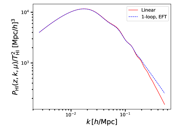
The difference between the linear and EFT power spectra is illustrated in Figure 1. A comprehensive review of the redshift-space counterterms and the free parameters associated with the EFT 1-loop power spectrum is given in [5].
2.3 HI IM bispectrum
For the HI bispectrum, i.e. the Fourier transform of the three-point function, we use a tree-level model with a phenomenological model of nonlinear RSD, following e.g. [35, 18]:
| (2.13) |
where the second-order redshift space kernels is given by:
| (2.14) |
where , ; and are the SPT kernels [6]; and the tidal kernel is [36, 31]. The RSD ‘fingers of god’ damping factor is [37, 38]
| (2.15) |
where characterizes the damping scale, with fiducial value given by the linear velocity dispersion . Note that we do not apply an ‘fog’ damping factor to the power spectrum since nonlinear RSD are treated by the EFT counter terms. Finally, the fiducial values of the stochastic terms in Equation 2.13 are [18]:
| (2.16) |
where is the effective number density and its is given by the HOD formalism used to derive the HI bias, as in [30].
2.4 Alcock-Paczynski effect
The Alcock-Paczynski (AP) effect relates the observed angular and redshift separations of objects to the actual cosmological distances, providing a means to investigate the large-scale structure of the universe. The AP effect is particularly significant in cosmological surveys and clustering analysis, as it allows us to infer information about the cosmological model and geometry of the universe. To implement this, we need a rescaling factor in the HI power spectrum and bispectrum.
The fiducial cosmology wavevector is related to the true wavevector by , where and as . The correlation function, being a dimensionless quantity, is left unchanged by this rescaling [15]. Thus leading to:
| (2.17) |
The fiducial Fourier coordinates are related to the true values as
| (2.18) | ||||
| (2.19) |
Extending Equation 2.18 and Equation 2.19 to 3 dimensions, we find that [39]:
| (2.20) |
This establishes the relationship between the observed and fiducial bispectra, accounting for the AP effect by considering the true and fiducial values of the Hubble parameter and angular diameter distance . Such a formalism is important for making precise measurements and extracting cosmological information from observations of large-scale structure.
2.5 HI IM window
The observational window of HI IM surveys is constrained by strong foreground contamination. We apply foreground avoidance filters in the plane [17, 15, 20]: (a) a cutoff to excise contaminated long-wavelength radial modes: ; and (b) avoidance of the foreground wedge, where spectrally smooth foregrounds leak into small-scale transverse modes:
| (2.21) |
Here is the comoving line-of-sight distance, is the number of primary beams away from the beam centre that contaminate the signal, and is the beam, with the dish diameter. We consider [20].
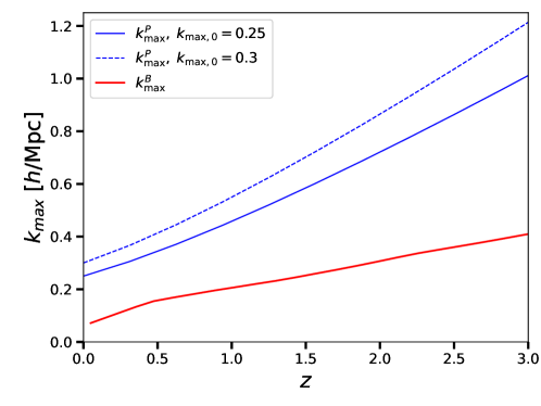
The minimum wavenumber, which corresponds to the largest scales probed by a survey of volume within a redshift bin, is , where being the fundamental frequency of the survey. The maximum wavenumber (corresponding to the smallest scale) is chosen for the tree-level bispectrum as [17]
| (2.22) |
where is the nonlinear scale set by the RMS displacement in the Zel’dovich approximation:
| (2.23) |
The EFT power spectrum probes mildly nonlinear scales with a higher . We assume that the maximum scale evolves as [40, 41]
| (2.24) |
where is the linear growth factor, normalised to unity at present (i.e. ). Following [42, 5, 43], we use
| (2.25) |
The small-scale cuts are shown in Figure 2.
3 Fisher forecast formalism
We use the Fisher information matrix [44, 45] to forecast precision on model parameters attainable by a HIRAX-like survey. The Fisher matrix for the power spectrum is (e.g. [17, 20])
| (3.1) |
where the sum is over . For the bispectrum it is:
| (3.2) |
where the above sum is over all the triangles formed by the wavevectors , while satisfying . The derivatives are performed over the model parameters .
We assume that the covariances in the Fisher matrix formalism are Gaussian and diagonal. Then the variances for the two correlators are [46, 47]
| (3.3) | ||||
| (3.4) |
where the bin size is chosen as and for equilateral, isosceles and non-isosceles triangles, respectively. In the case of the bispectrum, for degenerate configurations, , we multiply the variance by a factor of 2 [48, 49]. Note that higher values than those shown in Figure 2 may still give a reasonably accurate estimate of the power spectrum – but at the cost of increasingly non-Gaussian contributions to the power spectrum variance [50]. Non-Guassian contributions to the bispectrum occur more readily than in the power spectrum case. For this reason, even with our conservative choice of , we include higher-order corrections to the variance, as well as taking account of theoretical errors (see [18] for a discussion).
| Property | HIRAX |
|---|---|
| redshift | |
| [m] | |
| [km] | |
| [] | |
| [hrs] | |
| efficiency | 0.7 |
We consider a HI IM survey in interferometer mode, similar to the one proposed for HIRAX [51, 52, 53, 25] with specifications given in Table 1. The instrumental noise term that appears in the power spectrum of Equation 2.7, is assumed to be Gaussian and it is given in the case of an interferometer by [54, 55, 56]:
| (3.5) |
where is the integration time, the sky area, and the effective area, which is determined by the efficiency via . For the system temperature , we add the receiver temperature to the sky temperature , which is obtained from Appendix D of [57]. The baseline distribution presented in Appendix A of [20] is used here.
For the baseline model, we consider the CDM cosmological parameters, the AP parameters, the growth rate, the bias, the amplitudes of the EFT counter terms and the noise parameters to be free. The counter term and noise parameters are considered nuisance and are marginalised over for each correlator. The final parameter vector then is reduced to
| (3.6) |
We also consider the summed information from the power spectrum and bispectrum. In this case we sum the two Fisher matrices, without considering the cross-Fisher between the two correlators, which is assumed to be small, following [35]:
| (3.7) |
Finally, the total Fisher matrix is a sum over all redshift bins, assuming that the bins are independent. Note that during the summation we have to be careful to account for the fact that the redshift-dependent parameters change – so that they are effectively new parameters for each . As a consequence, the dimension of the total Fisher matrix
| (3.8) |
is much larger than the dimension of a single-bin matrix. This requires care in the marginalisation. Further details of the marginalisation and projection in parameter space may be found in [58].
We investigate two further cosmological models that extend CDM. The constant cosmological parameters for the 3 models are
| CDM | (3.9) | |||
| (3.10) | ||||
| (3.11) |
In order to find the final constraints on the above parameters we apply Jacobian transformations to the Fisher matrix that corresponds to the parameter space in Equation 3.6, after marginalising over the remaining bias parameters:
| (3.12) |
This will provide the final parameter constraints, from each correlator and their summed signal, in the form .
The fiducial values used for the cosmological parameters are drawn from Planck cosmic microwave background (CMB) measurements [59]: , , , , and . Fiducial values for the extended model parameters are , , and .
The Fisher matrix results are combined with the data on cosmological parameters obtained from the Planck satellite [59]. For this, we use the Markov chain that samples the posterior distribution, obtained from the Planck webpage111http://pla.esac.esa.int/pla/#cosmology. The covariance matrix is computed from the chains, specifically for the subset of parameters being analyzed. This matrix is then inverted to obtain the Planck 2018 Fisher matrix. The Fisher matrices of the power spectrum and bispectrum and their combination are then summed with the latter. The Planck likelihood is treated as a multivariate Gaussian, appropriate for the free cosmological parameters being studied.
The cosmological parameter results from Planck data include various cosmological models and provide results from MCMC exploration chains, best fits, and tables. Specifically, we use the CDM chains with baseline likelihoods based on plikHM_TTTEEE_lowl_lowE, which we sample using Getdist222https://getdist.readthedocs.io/en/latest/.
4 Results
Here we present and analyse the results derived from the Fisher matrices for the three cosmological models.
4.1 CDM
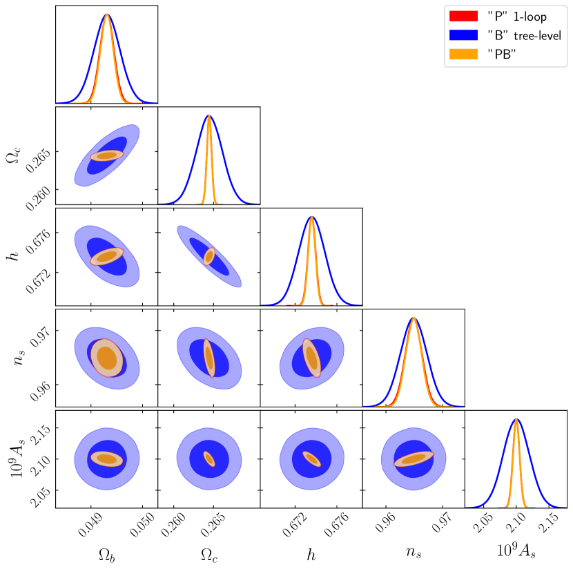
We expect the bispectrum to provide complementary information to the power spectrum. For CDM, Figure 3 shows that bispectrum constraints on cosmological parameters are weaker than from the EFT power spectrum. Nevertheless there are advantages from combining the 1-loop power spectrum and tree-level bispectrum as shown in Table 2. This combination enhances parameter constraints for the cosmological parameters , and . The constraints achieved with the combined analysis are notably more stringent than those derived from Planck 2018 CMB data.
We also find that the 1-loop power spectrum exhibits different correlations between parameters than the bispectrum. This indicates the possibility to break degeneracies and tightly constrain these parameters. The significant advantages in combining the two correlators is not evident here, due to the relatively small values considered for in the tree-level bispectrum analysis, compared to those used for the power spectrum EFT.
4.2 Modified gravity
The model provides a simple test of gravity: the fiducial value corresponds to the CDM and is a good approximation for simple non-clustering models of dark energy in general relativity. This means that a value of that deviates significantly from 0.55 indicates either a breakdown in general relativity on large scales, or a more complicated dark energy within the Friedmann-Lemaître-Robertson-Walker model (see e.g. [60]).
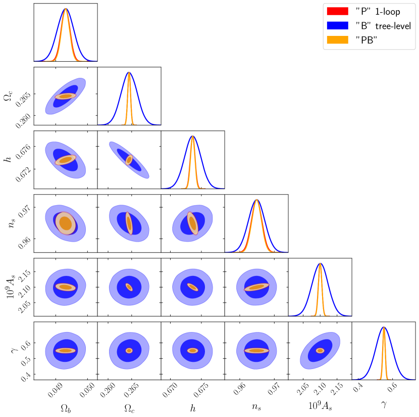
The 1-loop EFT power spectrum gives reasonable constraints for all considered cosmological parameters, while the bispectrum provides notably less stringent constraints for cosmological parameters and .
Constraints on the cosmological parameters in the model, are naturally weakened, compared to CDM, by the presence of a new free parameter which affects both the power spectrum and bispectrum. The EFT power spectrum provides stronger constraints on the growth rate compared to the bispectrum, as we show below in Figure 6. However the constraints do not simply translate to constraints, since arises in different ways in the two correlators, and since involves the cosmological parameters. Figure 4 shows that in fact, the EFT power spectrum gives better results than the tree-level bispectrum in constraining , while their combination delivers a notable improvement as shown in Table 2.
Figure 4 reveals the possibility to break parameter degeneracies, displayed as different orientation directions in the elliptical contours. Pushing the bispectrum analysis into smaller scales would have improved constraints, once the EFT power spectrum and tree-level bispectrum are combined.
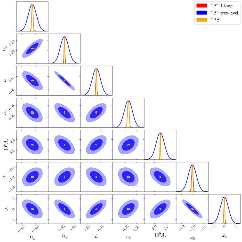
4.3 Dynamical dark energy
The model is a simple model often used to test for deviations from a cosmological constant that are due to dynamical (or evolving) dark energy (see e.g. [59]). Instead of choosing specific dynamical dark energy models, a two-parameter dark energy equation of state is used, providing some level of model independence.
With two additional parameters relative to CDM, we expect the constraints on cosmological parameters to worsen. This is confirmed by Figure 5. It is apparent that bispectrum constraints degrade even more than those from the power spectrum, where the latter provides more robust constraints to the dark energy parameters than the first. Despite the weakness of the bispectrum constraints, the combination with the power spectrum breaks degeneracies and leads to a noteworthy improvement in constraining , as shown in Table 2.
4.4 Summary of results on CDM, CDM and CDM
HIRAX P B P+B CDM 0.29 (0.27) 0.52 0.27 (0.25) 0.12 (0.11) 0.62 0.12 (0.11) 0.06 (0.05) 0.19 0.05 (0.05) 0.16 (0.15) 0.24 0.15 (0.13) 0.25 (0.24) 0.96 0.25 (0.24) 0.30 (0.28) 0.53 0.27 (0.26) 0.12 (0.11) 0.65 0.12 (0.11) 0.06 (0.05) 0.19 0.05 (0.05) 0.17 (0.16) 0.25 0.15 (0.15) 0.26 (0.25) 1.15 0.25 (0.24) 1.38 (1.30) 8.68 1.27 (1.22) 0.32 (0.29) 1.79 0.27 (0.26) 0.31 (0.27) 2.85 0.20 (0.18) 0.11 (0.10) 0.91 0.09 (0.08) 0.17 (0.15) 0.80 0.15 (0.14) 0.26 (0.25) 3.36 0.25 (0.24) 1.39 (1.22) 7.53 1.02 (0.93) 4.45 (3.91) 35.69 3.80 (3.41)
Table 2 summarises the 1 constraints on the 3 models, CDM, , and . It demonstrates that incorporating the bispectrum enhances the constraints on some parameters compared to using the power spectrum alone. This improvement is mainly evident for the and model parameters (i.e. , and ), while for cosmology the gain is minimal. To improve on the latter one would require to extract the bispectrum information from smaller scales, comparable to those used for the power spectrum analysis, by utilising the EFT framework.
Table 2 shows that there are only small changes in the power spectrum constraints on the cosmological parameters , , , and when moving from CDM to and . By contrast, there is a significant increase in error on (by a factor 1.73) for the bispectrum constraints in . In the model, the increase in bispectrum errors is even greater, and affects all 5 parameters. The increase in parameter uncertainties when transitioning from CDM to and arises due to the additional correlations introduced among variables as we increase the number of parameters in the model.
Table 2 shows the improvement in the power spectrum constraint when using the optimistic case Mpc compared to the pessimistic one (i.e. Mpc). This is due to the information that resides within the additional small scale modes. However, this improvement is marginal in the case of CDM and , unlike the dark energy model , which shows a more notable enhancement in the constraints. This is an indication that the information from the power spectrum saturates, as we venture to smaller scales, due to the thermal noise in the a HIRAX-like instrument.
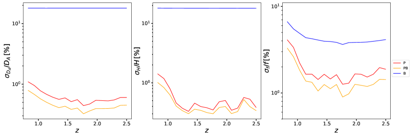
4.5 Distance and growth rate errors
In this section, we study the constraints on the angular diameter distance and the Hubble rate via the AP effect in the standard CDM model. We also compute errors on the growth rate .
The constraints are derived after marginalising over the nuisance parameters for both correlators, while the remaining model parameters are considered free (Equation 3.6). Figure 6 (upper panels) presents the results for the marginalized relative errors as a function of redshift.
The power spectrum delivers remarkably precise measurements, with an uncertainty of less than 1% across all redshift bins for the angular diameter distance and Hubble parameter , and within 1-2% for the growth rate . The bispectrum alone shows a lower precision, yielding relative errors within 10-20% for and , while for the growth rate the precision is 5%, across the redshift range. Consequently, incorporating the bispectrum into the analysis contributes a small improvement in precision on the BAO distance scale parameters and the growth rate.
4.6 Bias parameters
Clustering biases affect both the power spectrum and the bispectrum. Here we provide the constraints on biases as a function of redshift before marginalising them to get the cosmology constraints of the previous sections. The results are shown in Figure 6 (lower panels).
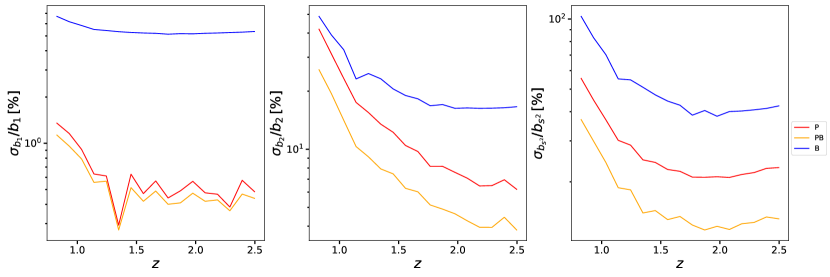
The power spectrum provides a precision of in most of the redshift range for the HI IM linear bias . The joint constraint from the two correlators is at the same level of precision as the power spectrum, indicating the poor performance of the bispectrum. The latter provides a 5% precision on constraints, which saturates beyond . For the quadratic bias and the tidal bias , the bispectrum provides a precision of 20% and 50% respectively, where the information saturates beyond . The power spectrum, on the other hand, exhibits an improvement in the constraints, reaching a precision smaller than 10% for , at high redshift bins, while for the relative errors saturate at 15% for . Combining the two correlators offers a significant improvement for these higher order bias parameters, reaching 4% and 5% at high redshifts for and respectively. This indicates the great potential offered by a joint EFT power spectrum and bispectrum analysis.
5 Conclusions
This work presents an analysis to estimate the cosmological precision possible with a HIRAX-like neutral hydrogen intensity mapping survey, using the 1-loop effective field theory power spectrum and the tree-level bispectrum. In addition to constraints on standard cosmological parameters, we estimate the uncertainties on modified gravity () and dynamical dark energy () parameters. Furthermore, we find the errors on the angular diameter distance , the Hubble rate and on the growth rate . Finally, we show the constraints on the linear and higher order clustering biases.
In order to remain within the domain of validity of the tree-level bispectrum and 1-loop EFT power spectrum, we have imposed appropriate scale cuts, as illustrated in Equation 2.22–Equation 2.25. For the EFT power spectrum, our baseline is a ‘pessimistic’ cut, with errors also computed for a more optimistic choice.
The 1 marginalised errors of our Fisher forecasts, from the whole redshift range, are summarised in Table 2. For CDM, the precision from P+B is sub-percent on the cosmological parameters , , , , and . For the extended models, and , these constraints naturally degrade, but the precision on the model parameters is high: 1.27% on the growth index and (1%, 3.8%) on (, ).
Compared to the tree-level power spectrum from our previous work [20], we find that EFT model improves precision on , , and , due to the additional information from small scales, as probed by the 1-loop power spectrum. However, this is not the case for and , which are less sensitive to this regime. The comparison with [20] also demonstrates the potential of the EFT power spectrum in breaking parameter degeneracies. This is clearly seen in the contour plots of Figure 3–Figure 5.
Finally, for the redshift-dependent parameters, we find a sub-percent precision for most redshifts on , and within 1-2% for most redshifts on (Figure 6, upper panels). The precision on the linear clustering bias is sub-percent, for most redshifts, while for the quadratic biases it reaches 5% from the joint analysis at high redshifts (Figure 6, lower panels).
The results presented in this work have relied on certain simplifications that, in a subsequent work, could be relaxed for a more comprehensive analysis. Introducing the 1-loop power spectrum covariance would make the constraints more realistic for future surveys, while extending the reach of the bispectrum, by using the 1-loop Effective Field Theory model (see e.g. [61]), would improve significantly its role in this joint analysis and subsequently the cosmological constraints.
Acknowledgements
The authors are supported by the South African Radio Astronomy Observatory and the National Research Foundation (Grant No. 75415).
References
- [1] L. Senatore and M. Zaldarriaga, Redshift Space Distortions in the Effective Field Theory of Large Scale Structures, 1409.1225.
- [2] R. E. Angulo, S. Foreman, M. Schmittfull and L. Senatore, The one-loop matter bispectrum in the effective field theory of large scale structures, 1406.4143.
- [3] S. Foreman and L. Senatore, The EFT of large scale structures at all redshifts: analytical predictions for lensing, Journal of Cosmology and Astroparticle Physics 2016 (2016) 033 [1503.01775].
- [4] G. d'Amico, J. Gleyzes, N. Kokron, K. Markovic, L. Senatore, P. Zhang et al., The cosmological analysis of the SDSS/BOSS data from the effective field theory of large-scale structure, Journal of Cosmology and Astroparticle Physics 2020 (2020) 005 [1909.05271].
- [5] M. M. Ivanov, Effective Field Theory for Large-Scale Structure, 2212.08488.
- [6] F. Bernardeau, S. Colombi, E. Gaztañaga and R. Scoccimarro, Large-scale structure of the Universe and cosmological perturbation theory, Phys. Rep. 367 (2002) 1 [astro-ph/0112551].
- [7] M. Cataneo, S. Foreman and L. Senatore, Efficient exploration of cosmology dependence in the EFT of LSS, JCAP 04 (2017) 026 [1606.03633].
- [8] A. Naskar, S. Choudhury, A. Banerjee and S. Pal, EFT of Inflation: Reflections on CMB and Forecasts on LSS Surveys, 1706.08051.
- [9] M. M. Ivanov, E. McDonough, J. C. Hill, M. Simonović, M. W. Toomey, S. Alexander et al., Constraining Early Dark Energy with Large-Scale Structure, Phys. Rev. D 102 (2020) 103502 [2006.11235].
- [10] R. Angulo, M. Fasiello, L. Senatore and Z. Vlah, On the statistics of biased tracers in the effective field theory of large scale structures, Journal of Cosmology and Astroparticle Physics 2015 (2015) 029 [1503.08826].
- [11] A. Perko, L. Senatore, E. Jennings and R. H. Wechsler, Biased tracers in redshift space in the eft of large-scale structure, 1610.09321.
- [12] T. Fujita, V. Mauerhofer, L. Senatore, Z. Vlah and R. Angulo, Very massive tracers and higher derivative biases, Journal of Cosmology and Astroparticle Physics 2020 (2020) 009 [1609.00717].
- [13] P. Zhang and Y. Cai, BOSS full-shape analysis from the EFTofLSS with exact time dependence, Journal of Cosmology and Astroparticle Physics 2022 (2022) 031 [2111.05739].
- [14] P. Carrilho, C. Moretti and A. Pourtsidou, Cosmology with the EFTofLSS and BOSS: dark energy constraints and a note on priors, Journal of Cosmology and Astroparticle Physics 2023 (2023) 028 [2207.14784].
- [15] N. Sailer, E. Castorina, S. Ferraro and M. White, Cosmology at high redshift — a probe of fundamental physics, Journal of Cosmology and Astroparticle Physics 2021 (2021) 049 [2106.09713].
- [16] A. Pourtsidou, Interferometric H i intensity mapping: perturbation theory predictions and foreground removal effects, Mon. Not. Roy. Astron. Soc. 519 (2023) 6246 [2206.14727].
- [17] D. Karagiannis, A. Lazanu, M. Liguori, A. Raccanelli, N. Bartolo and L. Verde, Constraining primordial non-Gaussianity with bispectrum and power spectrum from upcoming optical and radio surveys, MNRAS 478 (2018) 1341 [1801.09280].
- [18] D. Karagiannis, A. Slosar and M. Liguori, Forecasts on Primordial non-Gaussianity from 21 cm Intensity Mapping experiments, JCAP 11 (2020) 052 [1911.03964].
- [19] D. Karagiannis, J. Fonseca, R. Maartens and S. Camera, Probing primordial non-Gaussianity with the power spectrum and bispectrum of future 21 cm intensity maps, Phys. Dark Univ. 32 (2021) 100821 [2010.07034].
- [20] D. Karagiannis, R. Maartens and L. F. Randrianjanahary, Cosmological constraints from the power spectrum and bispectrum of 21cm intensity maps, Journal of Cosmology and Astroparticle Physics 2022 (2022) 003 [2206.07747].
- [21] SKA collaboration, D. J. Bacon et al., Cosmology with Phase 1 of the Square Kilometre Array: Red Book 2018: Technical specifications and performance forecasts, Publ. Astron. Soc. Austral. 37 (2020) e007 [1811.02743].
- [22] J. Wang et al., H i intensity mapping with MeerKAT: calibration pipeline for multidish autocorrelation observations, Mon. Not. Roy. Astron. Soc. 505 (2021) 3698 [2011.13789].
- [23] S. Cunnington et al., H i intensity mapping with MeerKAT: power spectrum detection in cross-correlation with WiggleZ galaxies, Mon. Not. Roy. Astron. Soc. 518 (2022) 6262 [2206.01579].
- [24] S. Cunnington et al., The foreground transfer function for H i intensity mapping signal reconstruction: MeerKLASS and precision cosmology applications, Mon. Not. Roy. Astron. Soc. 523 (2023) 2453 [2302.07034].
- [25] D. Crichton et al., Hydrogen Intensity and Real-Time Analysis Experiment: 256-element array status and overview, J. Astron. Telesc. Instrum. Syst. 8 (2022) 011019 [2109.13755].
- [26] F. Villaescusa-Navarro, M. Viel, K. K. Datta and T. R. Choudhury, Modeling the neutral hydrogen distribution in the post-reionization Universe: intensity mapping, JCAP 09 (2014) 050 [1405.6713].
- [27] J. Tinker, A. V. Kravtsov, A. Klypin, K. Abazajian, M. Warren, G. Yepes et al., Toward a Halo Mass Function for Precision Cosmology: The Limits of Universality, ApJ 688 (2008) 709 [0803.2706].
- [28] T. Lazeyras, C. Wagner, T. Baldauf and F. Schmidt, Precision measurement of the local bias of dark matter halos, J. Cosmology Astropart. Phys 2016 (2016) 018 [1511.01096].
- [29] A. Cooray and R. Sheth, Halo models of large scale structure, Phys. Rep. 372 (2002) 1 [astro-ph/0206508].
- [30] E. Castorina and F. Villaescusa-Navarro, On the spatial distribution of neutral hydrogen in the Universe: bias and shot-noise of the HI power spectrum, MNRAS 471 (2017) 1788 [1609.05157].
- [31] T. Baldauf, U. Seljak, V. Desjacques and P. McDonald, Evidence for quadratic tidal tensor bias from the halo bispectrum, Phys. Rev. D 86 (2012) 083540 [1201.4827].
- [32] R. A. Battye, I. W. A. Browne, C. Dickinson, G. Heron, B. Maffei and A. Pourtsidou, H I intensity mapping: a single dish approach, MNRAS 434 (2013) 1239 [1209.0343].
- [33] D. Blas, J. Lesgourgues and T. Tram, The cosmic linear anisotropy solving system (CLASS). part II: Approximation schemes, Journal of Cosmology and Astroparticle Physics 2011 (2011) 034 [1104.2933].
- [34] S.-F. Chen, Z. Vlah and M. White, The reconstructed power spectrum in the Zeldovich approximation, JCAP 09 (2019) 017 [1907.00043].
- [35] V. Yankelevich and C. Porciani, Cosmological information in the redshift-space bispectrum, Mon. Not. Roy. Astron. Soc. 483 (2019) 2078 [1807.07076].
- [36] P. McDonald and A. Roy, Clustering of dark matter tracers: generalizing bias for the coming era of precision LSS, J. Cosmology Astropart. Phys 8 (2009) 020 [0902.0991].
- [37] J. A. Peacock and S. J. Dodds, Reconstructing the linear power spectrum of cosmological mass fluctuations, Mon. Not. Roy. Astron. Soc. 267 (1994) 1020 [astro-ph/9311057].
- [38] W. E. Ballinger, J. A. Peacock and A. F. Heavens, Measuring the cosmological constant with redshift surveys, Mon. Not. Roy. Astron. Soc. 282 (1996) 877 [astro-ph/9605017].
- [39] Y.-S. Song, A. Taruya and A. Oka, Cosmology with anisotropic galaxy clustering from the combination of power spectrum and bispectrum, J. Cosmology Astropart. Phys 8 (2015) 007 [1502.03099].
- [40] T. Baldauf, M. Mirbabayi, M. Simonović and M. Zaldarriaga, LSS constraints with controlled theoretical uncertainties, 1602.00674.
- [41] A. Chudaykin, M. M. Ivanov, O. H. E. Philcox and M. Simonović, Nonlinear perturbation theory extension of the Boltzmann code CLASS, Phys. Rev. D 102 (2020) 063533 [2004.10607].
- [42] T. Steele and T. Baldauf, Precise Calibration of the One-Loop Trispectrum in the Effective Field Theory of Large Scale Structure, Phys. Rev. D 103 (2021) 103518 [2101.10289].
- [43] D. J. H. Chung, M. Münchmeyer and S. C. Tadepalli, Search for Isocurvature with Large-scale Structure: A Forecast for Euclid and MegaMapper using EFTofLSS, 2306.09456.
- [44] M. Tegmark, Measuring cosmological parameters with galaxy surveys, Physical Review Letters 79 (1997) 3806 [astro-ph/9706198].
- [45] M. Tegmark, A. J. S. Hamilton, M. A. Strauss, M. S. Vogeley and A. S. Szalay, Measuring the galaxy power spectrum with future redshift surveys, The Astrophysical Journal 499 (1998) 555 [astro-ph/9708020].
- [46] E. Sefusatti, M. Crocce, S. Pueblas and R. Scoccimarro, Cosmology and the bispectrum, Phys. Rev. D 74 (2006) 023522 [astro-ph/0604505].
- [47] E. Sefusatti and E. Komatsu, Bispectrum of galaxies from high-redshift galaxy surveys: Primordial non-Gaussianity and nonlinear galaxy bias, Phys. Rev. D 76 (2007) 083004 [0705.0343].
- [48] K. C. Chan and L. Blot, Assessment of the information content of the power spectrum and bispectrum, Phys. Rev. D 96 (2017) 023528 [1610.06585].
- [49] V. Desjacques, D. Jeong and F. Schmidt, Large-scale galaxy bias, Phys. Rep. 733 (2018) 1 [1611.09787].
- [50] K. C. Chan and L. Blot, Assessment of the Information Content of the Power Spectrum and Bispectrum, Phys. Rev. D 96 (2017) 023528 [1610.06585].
- [51] L. B. Newburgh et al., HIRAX: A Probe of Dark Energy and Radio Transients, Proc. SPIE Int. Soc. Opt. Eng. 9906 (2016) 99065X [1607.02059].
- [52] B. R. B. Saliwanchik, A. Ewall-Wice, D. Crichton, E. R. Kuhn, D. Ölçek, K. Bandura et al., Mechanical and optical design of the HIRAX radio telescope, in Ground-based and Airborne Telescopes VIII, vol. 11445 of Society of Photo-Optical Instrumentation Engineers (SPIE) Conference Series, p. 114455O, Jan., 2021, 2101.06338.
- [53] E. R. Kuhn, B. R. B. Saliwanchik, M. Harris, M. Aich, K. Bandura, T.-C. Chang et al., Design and implementation of a noise temperature measurement system for the Hydrogen Intensity and Real-time Analysis eXperiment (HIRAX), 2101.06337.
- [54] M. Zaldarriaga, S. R. Furlanetto and L. Hernquist, 21 Centimeter Fluctuations from Cosmic Gas at High Redshifts, ApJ 608 (2004) 622 [astro-ph/0311514].
- [55] M. Tegmark and M. Zaldarriaga, Fast Fourier transform telescope, Phys. Rev. D 79 (2009) 083530 [0805.4414].
- [56] P. Bull, P. G. Ferreira, P. Patel and M. G. Santos, Late-time cosmology with 21cm intensity mapping experiments, Astrophys. J. 803 (2015) 21 [1405.1452].
- [57] Cosmic Visions 21 cm collaboration, R. Ansari et al., Inflation and Early Dark Energy with a Stage II Hydrogen Intensity Mapping experiment, 1810.09572.
- [58] Euclid collaboration, A. Blanchard et al., Euclid preparation: VII. Forecast validation for Euclid cosmological probes, Astron. Astrophys. 642 (2020) A191 [1910.09273].
- [59] Planck Collaboration, N. Aghanim, Y. Akrami, M. Ashdown, J. Aumont, C. Baccigalupi et al., Planck 2018 results. VI. Cosmological parameters, A&A 641 (2020) A6 [1807.06209].
- [60] M. Ishak, Testing General Relativity in Cosmology, Living Rev. Rel. 22 (2019) 1 [1806.10122].
- [61] G. D’Amico, Y. Donath, M. Lewandowski, L. Senatore and P. Zhang, The one-loop bispectrum of galaxies in redshift space from the Effective Field Theory of Large-Scale Structure, 2211.17130.