Ring Gap Structure around Class I Protostar WL 17
Abstract
WL 17 is a Class I object and was considered to have a ring–hole structure. We analyzed the structure around WL 17 to investigate the detailed properties of WL 17. We used ALMA archival data, which have a higher angular resolution than previous observations. We investigated the WL 17 system with the 1.3 mm dust continuum and 12CO and C18O ( = 2–1) line emissions. The dust continuum emission showed a clear ring structure with inner and outer edges of 11 and 21 au, respectively. In addition, we detected an inner disk of 5 au radius enclosing the central star within the ring, the first observation of this structure. Thus, WL 17 has a ring–gap structure, not a ring–hole structure. We did not detect any marked emission in either the gap or inner disk, indicating that there is no sign of a planet, circumplanetary disk, or binary companion. We identified the base of both blue-shifted and red-shifted outflows based on the 12CO emission, which is clearly associated with the disk around WL 17. The outflow mass ejection rate is 3.6 and the dynamical timescale is as short as yr. The C18O emission showed that an inhomogeneous infalling envelope, which can induce episodic mass accretion, is distributed in the region within au from the central protostar. With these new findings, we can constrain the planet formation and dust growth scenarios in the accretion phase of star formation.
1 Introduction
Stars (or protostars) form in molecular cloud cores, and planets form in the course of star formation. The typical mass and density of molecular cloud cores are the order of with a H2 volume density of 104–106 cm-3 (e.g. Onishi et al., 2002; Tachihara et al., 2002; André et al., 2014; Tokuda et al., 2020). Protostars form in gravitationally collapsing cloud cores (Larson, 1969). Since the mass of a protostar at its birth is (Masunaga & Inutsuka, 2000), a remnant of the collapsing cloud core (or infalling envelope) with a mass of remains around the newborn star (Bate, 1998; Machida & Matsumoto, 2011). The protostar then grows by accretion from the infalling envelope (for details, see review by Tsukamoto et al., 2022). The mass accretion from the envelope lasts for about yr (Enoch et al., 2009) during which gas is supplied from the infalling envelope to the protostar through the circumstellar disk. The circumstellar disk also grows in the mass accretion phase (e.g., Tomida et al., 2017). Part of the envelope gas accretes onto the circumstellar disk and protostar, while the remainder is ejected by the protostellar outflow (Matzner & McKee, 2000; Machida & Hosokawa, 2013). After the infalling envelope is depleted, the circumstellar disk or protoplanetary disk gradually dissipates. Finally, the central object (protostar or pre-main sequence star) contracts on the Kelvin–Helmholtz timescale and hydrogen burning occurs, creating a main sequence star.
It has been considered that planet formation begins in the protoplanetary disk after the mass accretion phase ends (Hayashi, 1981; Hayashi et al., 1985). In other words, planet formation occurs in an isolated disk and the mass supply from the infalling envelope and mass ejection by the outflow are ignored. The first step of planet formation is dust growth (see review by Testi et al., 2014). Observations have confirmed sub-micron-sized dust grains in interstellar space and molecular cloud cores (Lada & Lada, 2003; Williams & Cieza, 2011). The collisional growth of such dust grains is possible in high-density regions (e.g., Kawasaki et al., 2022; Kawasaki & Machida, 2023). Past studies have found that it is difficult for dust grains to grow in gravitationally collapsing cloud cores (Ormel et al., 2009, 2011; Hirashita & Li, 2013). Note that some observations have also shown possible evidence of micron- and millimeter-sized dust in core and envelope scales (e.g., Miotello et al., 2014; Lefèvre et al., 2016). Recent theoretical studies indicate that the growth of dust grains with the size larger than millimeters is possible in circumstellar disks during the main accretion stage (Vorobyov et al., 2018; Tsukamoto et al., 2021; Ohashi et al., 2021; Koga & Machida, 2023). It is thus important to identify when planet formation or dust growth begins in the star formation process.
Recent observations imply that planet formation begins before the end of the accretion stage or Class 0/I stages (Tychoniec et al., 2020). In the following, we call a disk around a Class II object a protoplanetary disk and a disk around a Class 0 or I object a circumstellar disk. Tychoniec et al. (2020) have shown that there is insufficient dust to produce several planets in protoplanetary disks after the accretion phase. In addition, various structures such as rings, gaps, holes, and spiral designs have been confirmed in many protoplanetary disks (Andrews et al., 2018). These observations also imply that planet formation or dust growth may begin earlier than the Class II stage. Note that rings, gaps, holes, and spirals do not necessarily imply the existence of planets because a gravitationally unstable disk can form such features. It is difficult to observe signs of planet formation in circumstellar disks around Class 0 objects because such disks are still deeply embedded in dense gas envelopes. In addition, the disks around Class 0 objects tend to be massive and optically thick, making it difficult to detect forming planets. However, it is important to observe disks in the early stage of star formation to catch the first signs of planet formation.
Circumstellar disks around Class I objects are plausible sites for confirming the signs of planet formation because we can observe disks with less massive infalling envelopes (Manara et al., 2018; Williams et al., 2019; Sanchis et al., 2020; Mulders et al., 2020). In addition, a sufficient amount of dust remains in circumstellar disks around Class I objects (Tychoniec et al., 2020). Recent observations have shown a ring–gap or ring–hole structure in circumstellar disks around Class 0/I objects (Sheehan et al., 2020; Segura-Cox et al., 2020).
Our target WL 17 is a protostar in the Ophiuchus L1688 molecular cloud located 137 pc from the Sun (e.g., Ortiz-León et al., 2017, 2018). Enoch et al. (2009) and van Kempen et al. (2009) have shown that WL 17 is a Class I object. They estimated that the age of the protostar WL 17 is younger than 105 yr. Sheehan & Eisner (2017) also verified WL 17 as a Class I protostar by spectral energy distribution (SED) model fitting. They found that WL 17 has a ring–hole structure based on high angular resolution ALMA Band 3 observations, where the radius of the hole is au and the outer radius of the ring is au. Thus, the Class I object WL 17 should be a promising target for clarifying when planet formation and dust growth begin.
Although past observations have indicated that WL 17 is a Class I object, it is not usual for a Class I object to have a ring structure. In addition, some suspicious characteristics of the WL 17 system make it difficult to identify WL 17 as a Class I object. The bolometric luminosity of WL 17 is about 0.6 (Sheehan & Eisner, 2017), which is somewhat lower than typical Class I objects. Note that it has been well known since the 1990s that some Class I objects exhibit luminosities lower than (Kenyon et al., 1990).
In addition, N2H+, DCO+, and C18O line emissions, indicators of the system youth, were not detected around WL 17 in past studies (Loren et al., 1990; André et al., 2007; van Kempen et al., 2009). Then, using a single-dish telescope, van der Marel et al. (2013) showed a broad 12CO ( = 3–2) line emission, implying an outflow associated with WL 17. However, it is difficult to make conclusions about the outflow driven by the WL 17 system because of the insufficient spatial resolution. Thus, the presence of an outflow has yet to be confidentially confirmed around WL 17.
Class I objects are in the accretion phase, meaning that the infalling envelope encloses the central object. The typical accretion luminosity is expected to be – (Kenyon & Hartmann, 1995). In addition, the outflow is a useful indicator of gas accretion because the release of the gravitational energy of the accreting matter drives the outflow (Pudritz & Norman, 1986; Tomisaka, 2002). On the other hand, ring and hole structures are considered to appear in the later Class II evolutionary stage. Thus, more detailed observations of the WL 17 system would constrain the formation of substructures in the disk to the early phase of star and planet formation.
The aim of this study is to clarify the evolutionary stage and growth timescale of the substructure of WL 17 using two sets of high-resolution ALMA archival data. The data contain continuum and 12CO and C18O ( = 2–1) line emissions. Details of the data are presented in §2. In §3, we present the results of the continuum and 12CO line emissions and estimate the physical quantities of the WL 17 system, such as the gas mass and outflow mass ejection rate. In §4, we confirm the details of the remaining envelope gas around WL 17 with C18O line observation and Herschel’s H2 column density map. In addition, we discuss the possible process of substructure formation around WL 17 and suggest plausible scenarios to explain the WL 17 system in §4. We summarize our results in §5.
2 Observation Data and Imaging
2.1 High-resolution Continuum Observations
We used ALMA archival data (Project 2019.1.00458.S, PI Patrick Sheehan) to obtain high-resolution continuum images. The observations were carried out on 2019 September 29 using the ALMA main array in its C43-9/10 configuration. There were two continuum spectral windows with central frequencies of 218 GHz and 232 GHz in Band 6. Both had a bandwidth of 1.875 GHz.
The data were calibrated with the Common Astronomy Software Application (CASA; McMullin et al., 2007) version 6.2.1. We used only the tclean task in our imaging process. We applied Briggs weighting with a robustness parameter of 0.5 and an image grid of 00037. We performed self-calibrations and could not achieve any improvement because of the low signal-to-noise-ratio (100). The resultant synthesized beam size was ( au) with a position angle (PA) of at the distance of WL 17 (137 pc; Sheehan & Eisner, 2017), which is the highest resolution ever achieved for this source. The sensitivity of the continuum achieved was 18 Jy beam-1.
2.2 Molecular Line Observations
We used further ALMA archival data (Project 2019.1.01792.S, PI Diego Mardones) to investigate the gas structure around the protostellar disk. The observations were carried out on 2019 November 21 using the ALMA main array in its C-7 configuration. We used three spectral windows targeting the continuum, 12CO ( = 2–1), and C18O ( = 2–1). The continuum spectral window had a central frequency of 232 GHz and a bandwidth of 1.875 GHz. The 12CO and C18O line spectral windows had central frequencies of 230 and 219 GHz, respectively. The bandwidth of both windows was 11.7 MHz.
In the imaging process, we also used the CASA task tclean and applied Briggs weighting with a robustness parameter of 0.5, an image grid of 0140, and a velocity resolution of 0.1 km s-1. In addition, the continuum was subtracted from the 12CO and C18O line data using the CASA task imcontsub. The resultant synthesized beam size was ( au) with a PA of . We achieved a sensitivity of 0.33 mJy beam-1 for the continuum and 0.35 K per 0.1 km s-1 for the CO lines.
3 Results
3.1 High-spatial Resolution Continuum Image
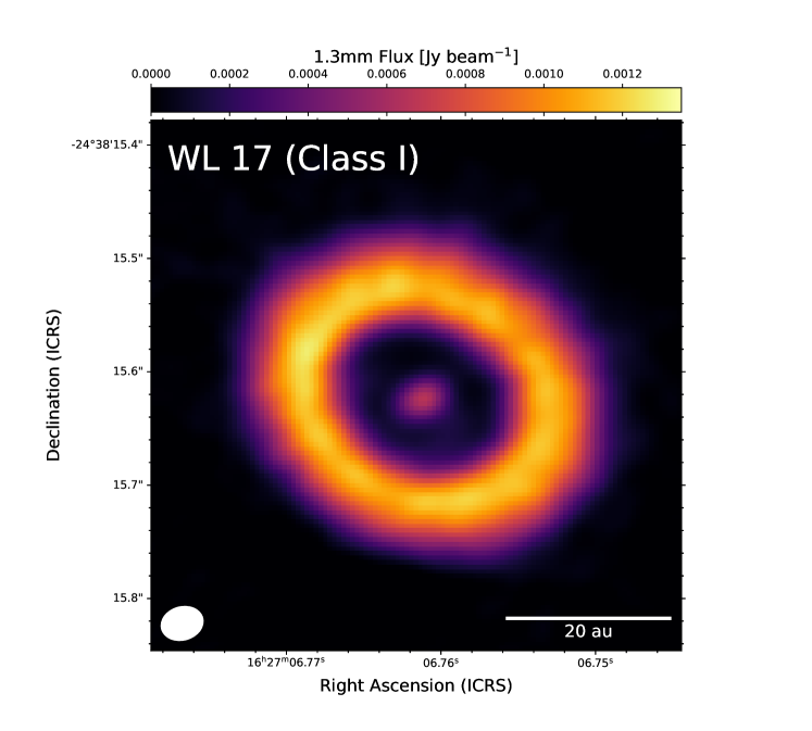
Figure 1 shows a 1.3 mm (Band6; 225 GHz) continuum image of WL 17 at an angular resolution of 0037 0031. The geometric mean of the major and minor axes of the beam is 1.6 times smaller than that in the previous 3 mm (Band 3; 97.5 GHz) observations (Sheehan & Eisner, 2017). We smoothed our 1.3 mm image into a lower-resolution image with a beam size of 006005, which is the same as in Sheehan & Eisner (2017). Then, we obtained the sensitivity of 21 Jy beam-1. Assuming a spectral index =2 (or ; Han et al., 2023), our imaging sensitivity can be equivalently converted into 4 Jy beam-1 at 3 mm, which is nine times higher than that in the previous 3 mm observation, 36 Jy beam-1. Although Sheehan & Eisner (2017) mentioned the intensity enhancement of the central position, the contrast between the central position and surrounding is marginal. Thus, they interpreted the inner structure as a hole with a radius of 13 au. In our study, the improved sensitivity and angular resolution clearly illustrate the presence of an inner disk, which is expected to enclose the central protostar. Thus, WL 17 has a ring–gap structure.
In the following, we refer to the inner dust disk and outer dust ring observed in the 1.3 mm continuum (Fig. 1) as the inner disk and the outer ring, respectively. We also use the term disk’ to describe the disk structure around WL 17. While the gas component of the disk around WL 17 has not been clearly resolved in molecular line emissions, it is expected to be present around the Class I object. In this paper, we consider the whole disk to contain undetected gas and dust, which are distributed to a large radius ( au). The inner disk and outer ring are part of the disk. In addition, the outflow is considered to be driven by the disk or the whole disk region.
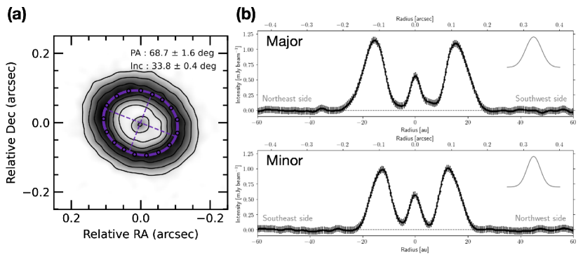
We fitted the outer ring with an ellipse and derived the inclination angle and position angle (PA) for the outer ring on the image shown in Figure 1, using the method adopted in Yamaguchi et al. (2021). The fitted ellipse is shown in Figure 2(a). We describe the fitting procedure in the following. First, we determined the radial peak position of the outer ring every 1∘ in the position angle (or vertical) direction from the intensity map on polar coordinates. Second, these collective peak positions were plotted on the continuum intensity map (purple broken line in Fig. 2a). Using the major and minor axes of the ellipse (or the purple broken line), we estimated an inclination angle of 33.8∘ and a PA of 68.7∘, as shown in Figure 2(a), indicating that we observed the WL 17 system nearly face-on.
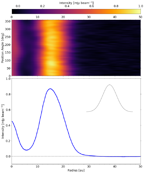
Figure 2(b) shows the intensity profiles in the major- and minor-axis directions. The size of the outer ring is measured to be 56 46 au with PA = 68.7∘. Using the derived ellipse fitting parameters and PA, we deprojected the 1.3 mm continuum image of the disk. As shown in the top panel of Figure 3, we created the intensity map on polar coordinates from the deprojected image. The azimuthally averaged radial intensity profile is plotted in the bottom panel of Figure 3. The uncertainty in the radial profile can be evaluated as the error of the mean at each radius, with a value of mJy beam-1. We adopted the Gaussian fitting to the peaks of the inner disk and the outer ring shown in Figure 3 and estimated the full width at half maximum (FWHM) without the beam deconvolution. The deconvolved size in the FWHM of the inner disk is 5.2 au. The size of the inner disk is comparable to the beam size, making it difficult to resolve its internal structure. Thus, for the inner disk, we consider the estimated FWHM ( au) as the upper limit of the radius. On the other hand, the peak radius of the outer ring is 15.7 au and the FWHM is 8.8 au, suggesting that the outer ring can be resolved spatially (the inner and outer edge radius of the outer ring are 11 and 21 au, respectively). Furthermore, we could not detect any strong thermal dust emission within the gap between the outer ring and inner disk in the range of – au even in the high-spatial-resolution image (Fig. 3 top). Figures 2 and 3 indicate that the intensity of thermal dust emission in the gap is significantly lower than that of the outer ring. Thus, there is a very high-intensity contrast between the gap and the outer ring.
We measured the total flux emitted from the ring–gap structure of WL 17 system (Fig. 1) considering the dust emission larger than 5 ( = 18 Jy beam-1). The total flux is 10-2 Jy, which is the sum of the inner disk (6.610-4 Jy) and outer ring (4.310-2 Jy). Thus, the flux from the outer ring is much greater than that from the inner disk. With the total flux , we estimated the dust mass seen in Figure 1 to be
| (1) |
where the dust is assumed to be optically thin, and a dust opacity at 1.3 mm of cm2 g-1 (Beckwith et al., 1990) and a dust temperature of K were adopted. The total dust mass was estimated to be =7.410. Adopting a gas-to-dust mass ratio of 100, the outer ring mass of WL 17 is at least , which is comparable or smaller than the dust ring mass estimated in previous studies ( for Sheehan & Eisner 2017). Note that we only estimated the mass of the outer ring shown in Figure 1. Thus, in our estimate should be the lower limit of the disk mass around WL 17 (see also §4.5). The outer ring mass around WL 17 estimated in this study is comparable to or slightly smaller than the disks around Class I objects (Fiorellino et al., 2022).
We compare the properties of the inner disk of the WL 17 system with those of other inner disks of objects associated with the ring–gap structure presented in Francis & van der Marel (2020). Note that the main targets of Francis & van der Marel (2020) are not circumstellar disks but protoplanetary disks. The radii of the inner disks shown in Francis & van der Marel (2020) are mainly distributed in the range – au, which is consistent with the radius of the WL 17 system (5 au). The fluxes for the inner disks reported in Francis & van der Marel (2020) are also comparable to that for the WL 17 system. Thus, the size and flux (or mass) for the WL 17 system are in good agreement with those for the other inner disks in Francis & van der Marel (2020). The flux ratio for the outer ring to the inner disk of the WL 17 system is also consistent with those in Francis & van der Marel (2020). The WL 17 system and other systems (or objects) are different with regard to their ratio of inner disk radius to outer ring radius. The ring radii for the systems in Francis & van der Marel (2020) range from 31 to 258 au, with an average of 102.2 au and a median of 84 au. On the other hand, the outer ring radius (or outermost radius of the ring) is 21 au for the WL 17 system, smaller than those for the systems reported in Francis & van der Marel (2020), suggesting that WL 17 may be younger than the other objects (for relevant discussion, see §4.3.3). Note that the sample from Francis & van der Marel (2020) is biased to larger and brighter protoplanetary disks, and the median disk size in Ophiuchus is smaller than that in their sample. Thus, further samples may be necessary to discuss the youth of the disks.
3.2 12CO Line Emission and Blue- and Red-shifted Outflows
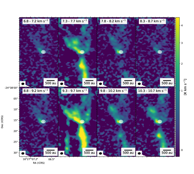
Figures 4 and 5 show the channel maps of the 12CO ( = 2–1) emission. Figure 6 represents the moment 0 maps of the 12CO ( = 2–1) emission. In Figures 4–6, we can confirm a cavity-like structure expected to be produced by a protostellar outflow. We also determined the outflow velocity using the position velocity (PV) diagrams (for details, see Fig. 7). We call the structure shown in Figure 4 the blue-shifted outflow and that in Figure 5 the red-shifted outflow. The blue-shifted outflow extends southeastward toward the central object (black contours) in Figure 4. On the other hand, we can confirm that the red-shifted outflow cavity extends in the north direction (Fig. 5). In addition to the cavity-like structure, we can also see a 12CO emission extending south toward the central object in Figure 5. Although we cannot clearly explain the emission in the south direction, it may be a secondary outflow (for details, see §4). The bases of the blue-shifted and red-shifted outflows are clearly superimposed on the white contour (dust continuum emission) in Figures 4 and 5. Thus, we could confirm that both the blue- and red-shifted outflows (or outflow cavities) are associated with the disk (or outer ring and inner disk) observed in the 1.3 mm continuum emission (Fig. 1).
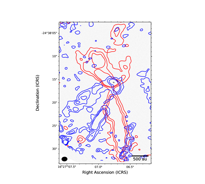
Figure 7 (a) and (c) also show the integrated intensity (or moment 0) maps of the blue-shifted (left) and red-shifted (right) 12CO outflows. Both the blue-shifted and red-shifted components show collimated (or narrow) flows enclosed by a cavity-like structure (Figure 6). As described above, the outflow directions (red-shifted and blue-shifted components) expected from the cavity-like structure are not exactly aligned each other. The outflow direction is in the southeast for the blue-shifted component, while it is in the northeast direction for the red-shifted component. Different direction outflows around a single embedded protostar can be seen in recent three-dimensional simulations (e.g., Matsumoto et al., 2017) and observations (Okoda et al., 2021; Sato et al., 2023). When an inhomogeneous infalling envelope encloses the disk, the propagation directions of the outflows differ, as described in Matsumoto et al. (2017). In addition, more than one pair (blue-shifted and red-shifted) of outflows can appear in different directions when the circumstellar disk is enclosed by an inhomogeneous infalling envelope (Hirano et al., 2020; Machida et al., 2020).
3.3 Outflow Physical Quantities
A large-scale outflow has been observed around WL 17, as described in §1. Using the 12CO ( = 3–2) emission obtained from the James Clerk Maxwell Telescope, van der Marel et al. (2013) found a strong outflow that seems to be associated with the WL 17 system, and they estimated the outflow properties. The blue-shifted component has a length of au, a mass of , and a maximum outflow velocity of . The red-shifted outflow component has au, , and . The averaged dynamical timescale of the outflow is yr. The total mass ejection rate is . The spatial resolution was not sufficient to identify the driving source of the outflow in van der Marel et al. (2013), and hence it is difficult to clearly state that the WL 17 system drives an outflow.
In this study, we could confidently confirm the base of the outflow with high spatial resolution observations. The outflow originates from the ring–gap structure around WL 17. The blue-shifted (Fig. 7a) and red-shifted (Fig. 7c) outflows detected in the 12CO emission are shown in the left panels of Figure 7, in which the areas surrounded by white lines indicate outflow areas with intensities exceeding 0.5 K km s-1. We estimated the physical properties of the outflows around WL 17 in the same manner as in van der Marel et al. (2013).
The lengths of the blue-shifted () and red-shifted () outflows are almost the same and are 2.4103 au in size. Note that we expect that the outflow extends further from the field of view in Figures 4 and 5, because the outflow lengths estimated in our study are several times smaller than those in van der Marel et al. (2013). Thus, we cannot estimate the actual length of the outflow with these figures due to the limited field of view. It is likely that Figures 4 and 5 show a recent (or latest) mass ejection event. In the following, we estimate the physical quantities of the recent mass ejection event with .
We estimate the outflow dynamical timescale using the outflow length and the maximum outflow velocity . We determined the outflow maximum velocity with the system velocity 4 km s-1 (van der Marel et al., 2013). To investigate the outflow (maximum) velocity, we generated PV diagrams along both the blue- and red-shifted outflows (Fig. 7b and d), from the regions bounded by the two arrows in Figure 7b and d.
The PV diagrams show that the high-velocity components are located around the dust continuum emission near the center. The region where the dust continuum emissions are detected is bounded by the gray broken lines in the PV diagrams. We also plotted the Keplerian velocity profile assuming protostellar masses of 1 and 2 on the PV diagrams. The velocities within the gray broken line can be attributed to Keplerian rotation, assuming a protostellar mass of –. We used a protostellar mass of for calculating the physical quantities for the WL 17 system below.
Although the velocities just outside the dust continuum emission seem to significantly exceed the Keplerian velocity of 2 , it is difficult to identify the origin of the high-velocity components near the dust continuum emission. The high-velocity emissions near the center could be composed of both Keplerian motion and high-velocity outflow (or jet). Thus, we excluded the high-velocity emissions near the region bounded by the gray broken lines when estimating the outflow velocity.
We can also see high-velocity components far from the dust continuum emission (or outside the region bounded by the gray broken lines). In both the red- and blue-shifted outflows, we could detect emissions of 2–5 about au distant from the emission peak for the dust continuum (Fig. 7). With the PV diagrams, we determined the maximum velocity of the blue-shifted () and red-shifted () components as 2.0 and 3.5, respectively. Then, we adopted the velocity for each blue- and red-shifted outflow to calculate the mass outflow rate. Thus, the outflow rate estimated in this study could be smaller than the actual outflow rate (for details, see below). The dynamical timescale can be calculated as
| (2) |
where is the inclination angle of the outflow () and the dynamical timescales of the red-shifted and blue-shifted outflows are estimated using the maximum velocity of the blue-shifted () and red-shifted () components, respectively. The outflow length, maximum velocity, and dynamical timescale are summarized in Table 1. The average of the dynamical timescale between the blue-shifted and red-shifted outflows is 3.0 yr, which is about two times shorter than that derived in van der Marel et al. (2013). Thus, it is expected that the outflow shown in Figures 4 and 5 and van der Marel et al. (2013) was ejected in the recent period 103–104 yr.

| Outflow | |||||
|---|---|---|---|---|---|
| ( au) | () | ( yr) | ( ) | ( yr-1) | |
| Blue lobe | 2.4 | 2.0 | 3.8 | 1.4 | 0.4 |
| Red lobe | 2.5 | 3.5 | 2.2 | 7.2 | 3.2 |
| Total | - | - | - | 8.7 | 3.6 |
Next, we estimate the outflow mass as , where , , , and are the mean molecular weight of H2 (), the hydrogen atom mass, the outflow area, and the average column density of H2 in the area, respectively. We convert the 12CO integrated intensity to the H2 column density using the factor, where . A factor of is adopted (Bolatto et al., 2013). The total mass of the blue-shifted and red-shifted outflows is 8.710 (see also Table 1). The outflow mass derived in this study is comparable to that in van der Marel et al. (2013).
The protostellar mass of the WL 17 system can be estimated to be 1–2 from the Keplerian velocity (for details, see Fig. 7). Thus, the WL 17 system does not contain very low-mass objects, such as a proto-brown dwarf. Note that very low-mass objects are considered to have low immensities () even in the Class 0 stage. Assuming a constant mass loss rate of the outflows, we estimated the total mass loss rate (sum of the red and blue shifted outflows) of 3.610-7 yr-1, as described in Table 1. This mass loss rate is several times larger than that in van der Marel et al. (2013). The mass outflow rate 3.610-7 yr-1 estimated in our analysis is smaller than that for typical Class 0 objects (Nagy et al., 2020; Feddersen et al., 2020). Note that the mass outflow rates for Class 0 objects are the largest among objects with different evolutionary stages (Class 0, I, Flat, and II objects) and they decrease as the protostellar systems evolve (e.g., Bontemps et al., 1996). We do not intend to claim that WL 17 is a very young, Class 0 object, but rather that it should be considered to be in the (later) accretion phase because the outflow physical parameters are similar to those for Class I (or Flat) objects. As described in Sheehan & Eisner (2017), the bolometric luminosity of WL 17 is estimated to be , which is comparable to that of Class I, Flat, and II objects (Watson et al., 2016).
4 Discussion
4.1 Remaining Mass of Core and Envelope around WL 17
We need to confirm the amount of mass in the infalling envelope to constrain the timescales of disk growth and ring formation, as described in §4.2. Thus, in this subsection, we discuss the remaining mass of the core and envelope around WL 17.
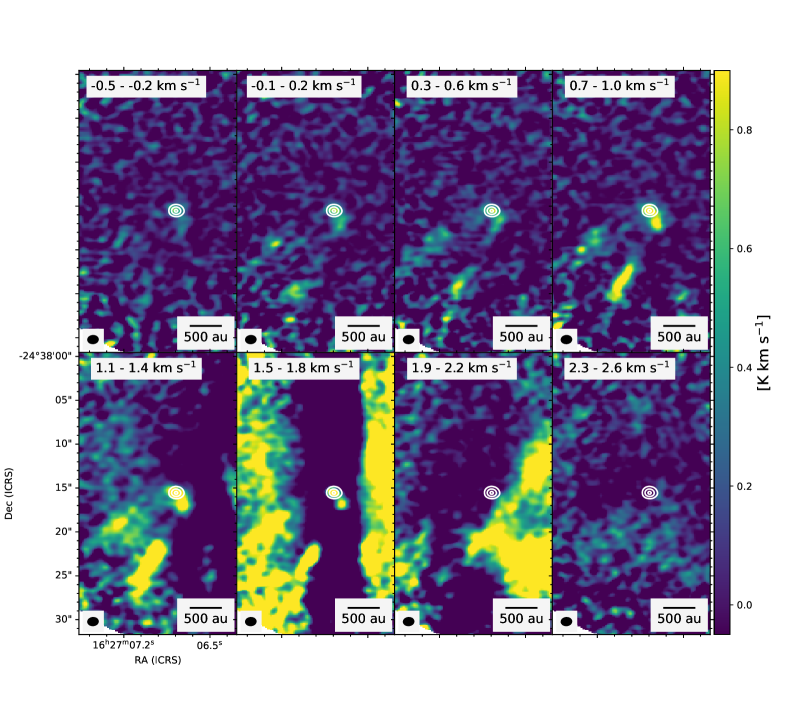
As described in §3.2, the outflow is associated with the WL 17 system. Considering that the outflow is powered by the accreting matter, it is expected that there is remaining infalling or envelope mass in the vicinity of the WL 17 system. To investigate the envelope around WL 17, Figure 8 shows the C18O emission that can trace the high-density gas. Figure 8 shows that the distribution of C18O emission is asymmetric and seen primarily to the north of the object, rather than enclosing it. The figure also indicates the existence of high-density gas in the region au around the central object WL 17. In addition, although the C18O emission can be detected at the peak position of the 1.3 mm dust continuum emission, the emission is not very strong. The C18O emission in the region within au from the central object is also not strong. Thus, Figure 8 indicates that envelope gas still remains around the WL 17 object, while the gas distribution is not homogeneous. In the last decade, ALMA observations revealed a protostellar system with inhomogeneous envelope structures (Pineda et al., 2022) where the rotationally supported disk is detached from the surrounding dense material (e.g., Tokuda et al., 2017). Although the origin of such complex systems is still debated (e.g., Matsumoto et al., 2015; Tokuda et al., 2018; Pineda et al., 2022), numerical simulations by Matsumoto et al. (2017) and Kuffmeier et al. (2017) demonstrated that the inhomogeneous distribution of the envelope gas could induce a time-variable accretion and mass ejection.
Assuming a protostellar mass of , the freefall velocity of the gas distributed about au from the central object can be estimated to be . Thus, the envelope gas seen in Figure 8 could fall within yr. Therefore, mass accretion would last for at least a further – yr which is shorter than the lifetime of Class 0/I objects (Enoch et al., 2009). Note that we estimated the required time using the location of WL 17 and C18O emission projected on the plane of the sky.
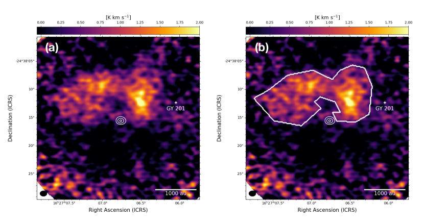
Figure 9 shows the column density map derived from the Herschel Gould Belt Survey data (André et al., 2010) with a resolution of 18 (Ladjelate et al., 2020). The figure indicates that WL 17 is located within a large-scale filamentary structure with a length of pc and width of 0.1 pc (Fig. 9 left). Within the filament, there are some clumps and young stellar objects (YSOs). We can see a small high-density clump with a size of – au associated with WL 17 (Fig. 9 right). Although the column density outside the core where WL 17 is embedded is relatively low, that of the WL 17 core is high. As seen in Figure 9(b), GY 201 is located close to WL 17. However, the dense gas traced by C18O (Fig. 8) seems to be associated with WL 17. Thus, although not all the matter shown in the right panel of Figure 9 would accrete onto the WL 17 system, a non-negligible amount of the matter is associated with the WL 17 system. Therefore, based on the outflow detection, the C18O distribution around WL 17 and the Herschel data, we expected that WL 17 is in the accretion phase of star formation.
We measured the remaining (or envelope) mass around WL 17. We estimated the mass of molecular hydrogen (H2) using the C18O column density. First, we need to determine the optical depth , which can be calculated using the following equation (Frerking et al., 1982):
| (3) |
where is the Planck constant, is the Boltzmann constant, represents the spectral frequency (=220 GHz), and denotes the excitation temperature, which is assumed to be 10 and 20 K. corresponds to the brightness temperature obtained from the observed data in C18O, which is around 1.1 K. We performed a Gaussian fit of the spectra in the area of Figure 8 (b) and used the FWHM as the velocity width km s-1). With the derived optical depth and the velocity width , we can estimate the C18O column density as
| (4) |
where we assume that the line spectrum has the Gaussian velocity dispersion, the is the dipole moment and is the energy level (Frerking et al., 1982). The C18O column density is then converted to the averaged H2 column density using the relation (Frerking et al., 1982). Finally, we calculate the converted H2 mass as follows:
| (5) |
where (= 2.8) is the mean molecular weight of H2 (Kauffmann et al., 2008), is the proton mass and is the area enclosed by the thick white line in Figure 8(b). The mass of molecular hydrogen estimated from C18O is . We can also estimate the mass of molecular hydrogen using the Herschel column density maps shown in Figure 9(b) with equation (5). We calculated the mass within each black circle in Figure 9(b), which have radii of 1000, 2000, and 3000 au, respectively. Because the WL 17 system is located in the filament, the H2 profile cut in the southwest direction across WL 17 has a sharp decline and a flat distribution at 1.51022 cm-2. The flat (column) density is widely distributed in the region 0.1 pc away from WL 17, where 0.1 pc corresponds to the typical dense core size and filament width (e.g., Onishi et al., 2002; Arzoumanian et al., 2011; Tokuda et al., 2019). Therefore, we treated the column density of 1.51022 cm-2 as the background level. The enclosed mass within these radii are listed in Table 2.
The total mass of molecular hydrogen in the vicinity of WL 17 is as small as –(Table 2). Note that, within au, the molecular hydrogen mass estimated from the C18O emission seems to be significantly smaller than that from Herschel column density. This difference can be partly attributed to missing flux in the ALMA observation (e.g., Tokuda et al., 2018). Furthermore, the inhomogeneous distribution of CO emission (Fig. 8) can also cause the difference in the estimated molecular hydrogen masses from the ALMA and Herschel observations. However, a substantial amount of mass () remains in the envelope within 2000–3000 au of WL 17 (Table 2). Although a Class II source GY 201 may be embedded in the same condensed gas region around WL 17, Figures 8 and 9 suggest that the dense gas is primary associated with the WL 17 system. Thus, mass accretion onto WL 17 is expected to continue in future evolutionary stages. The remaining mass surrounding the WL 17 system () is relatively small compared to the protostellar mass of WL 17 (). Therefore, we expect that the WL 17 system is in the late stage of the Class I phase, indicating the end of the mass accretion stage.
| Calculation area | ||||
|---|---|---|---|---|
| (1022 cm-2) | (107 au2) | () | ||
| C18O (=10 K) | White-line area in Figure 8 (b) | 0.4 | 0.3 | 4.410-3 |
| C18O (=20 K) | White-line area in Figure 8 (b) | 0.3 | 0.3 | 3.610-3 |
| H2 | Black circle (a) in Fig. 9, au | 1.0∗ | 0.3 | 1.010-2 |
| H2 | Black circle (b) in Fig. 9, au | 1.0∗ | 1.3 | 5.510-2 |
| H2 | Black circle (c) in Fig. 9, au | 0.9∗ | 2.8 | 1.110-1 |
| . The averaged H2 column density has been background subtracted (the background level1.51022 cm-2). | ||||

4.2 Disk Growth Timescale
In this subsection, we discuss the disk growth timescale during the mass accretion phase in terms of star formation. Ring and gap structures are usually observed in Class II objects. For Class II objects, the envelope is already depleted and the mass accretion and outflow rate are as low as yr-1 (Hartmann et al., 1998). Thus, it is considered that mass transfer from the envelope onto the disk has already been completed for Class II objects. Assuming a disk mass of and a mass accretion rate onto the disk from the envelope of yr-1 for Class II objects, the disk growth timescale is yr. In addition, the dissipation timescale of protoplanetary disks is considered to be – yr (Fedele et al., 2010). Thus, we can consider that the ring and gap structures form within – yr around Class II objects.
On the other hand, when the mass accretion rate onto the disk is high, as in Class 0 and I objects, the disk grows in a short time. Since the ring and gap structure could be related to dust growth and planet formation, it is crucial to specify when dust growth and planet formation begin. Therefore, it may be valuable to properly identify the evolutionary stage of WL 17 in order to constrain the timescale for ring and gap formation, as described in §1. Although various mechanisms have been proposed for the formation of ring and gap structures, we focus on the dynamic formation of ring and gap structures in an early or accretion stage of star formation.
During the mass accretion phase, the disk mass continues to increase due to the continuous mass supply from the infalling envelope. However, the disk cannot possess a large amount of mass because the disk becomes gravitationally unstable, and the disk material, composed of gas and dust, rapidly accretes onto the central protostar. Thus, the disk material is replaced on a short timescale (or disk growth timescale). Even if the dust ring is formed, it will fall onto the central protostar with the gas component when the rapid mass accretion induced by gravitational instability occurs. Thus, even if the ring and gap form in the mass accretion phase, they will only survive only within the disk growth timescale, during which all the disk material (gas and dust) should be replaced (for details, see the review by Tsukamoto et al., 2023).
When the mass accretion rate from the envelope to the disk is high, the time required for ring and gap formation becomes short. Note that the ring and gap must form before the pre-existent disk material is replaced by the newly accreting matter as described above. The mass accretion rate is assumed to be 10 times the mass loss rate , where is adopted (Cabrit, 2009; Konigl & Pudritz, 2000). Thus, with the mass outflow rate derived in §3.3, the mass accretion rate is estimated to be . Although the mass accretion rate derived from the outflow rate is 3.6 yr-1 with , we conservatively use in the following order of magnitude analysis. Assuming a disk mass of , the disk growth timescale is as short as yr, indicating that the accreting matter replenishes the disk within yr. In this case, rapid formation of the ring and gap structure (outer ring and inner disk) is required because the gas and dust within the disk are replaced by the accreting matter roughly every yr. Part of the disk gas is ejected by the outflow and the remainder falls onto the central star. Note that if the original disk matter remains within the disk without falling, the disk mass continues to increase as mass accretion proceeds. Then, gravitational instability occurs, which rapidly enhances the mass accretion rate onto the central star from the disk, as described above. As a result, the disk mass during the main mass accretion phase (or Class 0/I stage) is adjusted so as to balance the accreting matter from the envelope and the matter falling onto the central star (Tomida et al., 2017). In other words, fresh gas and dust continue to feed the disk, while those of the previous generation are pushed into the central star. Thus, the gas and dust cannot stay in the disk for a long time with a high mass accretion rate. Therefore, when a ring and gap structure appears in the accretion stage (or Class 0/I stage), we can severely constrain the timescale for dust growth and planet formation.
4.3 Possible Formation Scenarios for Ring Gap Stricture around WL 17
In this study, for the first time, we discovered an inner disk around WL 17 enclosed by the ring–gap structure. In addition, we found that an outflow is associated with the WL 17 system based on the 12CO emission, and the mass ejection rate due to the outflow is comparable to those for Class I objects. We also confirmed that the infalling envelope remains around the WL 17 system. Furthermore, we did not detect any strong emission or noticeable structure within the gap. With these new findings, we constrain the evolutionary stage and formation process of the ring–gap structure. In the following, we introduce and discuss four possible scenarios for the production of the ring–gap structure around WL 17: embedded binary system, unseen protoplanet, dispersal by disk wind, and dust growth front.
4.3.1 Embedded Binary System
First, we discuss the scenario for ring–gap formation by a binary system. When a binary system exists in a high-density region (or is embedded within an inner disk), the gravitational torque due to the binary orbital motion produces a non-axisymmetric structure that can transport the angular momentum outward. As a result, a ring–gap-like structure can form in a region outside the binary system, as shown in observations (e.g., Takakuwa et al., 2017) and numerical simulations (e.g., Matsumoto et al., 2019). For this scenario, a non-axisymmetric structure should appear outside the binary system to enhance the mass accretion and produce a gap (Machida et al., 2009; Matsumoto et al., 2019). Thus, a spiral-like structure corresponding to the channel flow to the binary system should be detected within the ring or gap. In addition, it is expected that the emission (or density distribution) of the ring-like structure is not uniform because the binary motion disturbs the circumbinary disk (Saiki & Machida, 2020). The ring enclosing the binary system corresponds to the circumbinary disk in this scenario. Circumbinary disks tend to appear in the embedded phase of star (or binary) formation because the mass of the circumbinary disk can be supplied from the infalling envelope.
In Sheehan & Eisner (2017), the region inside the ring or gap cannot be sufficiently resolved. Thus, with their observation, it is difficult to entirely reject the existence of a spiral structure created by the binary system in the gap region. On the other hand, we could detect neither a clear spiral nor non-axisymmetric structure in the gap. In other words, we could not confirm any sign of a binary system in the high-spatial-resolution image shown in Figure 1. However, we could not resolve the inner disk with a sufficiently high spatial resolution. In addition, if a binary system is embedded in the inner disk, it is possible for the secondary outflow described in §3.2 to be driven by a binary companion (Kuruwita et al., 2017; Saiki & Machida, 2020). Thus, although we cannot completely disprove the existence of a very close binary embedded in the inner disk, the embedded binary scenario is not plausible for explaining the ring–gap structure around WL 17.
4.3.2 Unseen Protoplanet
The most straightforward scenario to explain the ring–gap structure is a protoplanet in the gap. When a protoplanet orbits in a disk, a gap forms around the planet orbit (Kanagawa et al., 2015, 2016; Dipierro & Laibe, 2017). The detection of a circumplanetary disk in a gap or hole is strong evidence of the existence of a protoplanet. Recently, a circumplanetary disk was detected around PDS 70 (Keppler et al., 2018; Bensity et al., 2021) and two protoplanets (or circumplanetary disks) could be confirmed. The structure of PDS 70 is similar to that of WL 17. The PDS 70 system has a ring–gap structure in which an inner disk has also been detected. Although no circumplanetary disk could be detected in the gap around WL 17, it might be seen in future observations with higher sensitivity and spatial resolution. In addition, it is possible for a small planet with a mass of several Earth masses to produce a ring–gap structure when the disk viscosity is considerably small (Muto et al., 2010; Pérez et al., 2019). For example, Crida et al. (2006) showed that the gap opening mass for an inviscid disk can be described as
| (6) |
where , , and are the planet mass, protostellar mass, disk scale height, and radius, respectively (see also Muto et al., 2010). Thus, a small planet can create a gap depending on the disk parameters. Therefore, even if we do not detect a circumplanetary disk in the gap with future observations, we cannot reject the scenario in which a (small-sized) protoplanet is embedded within the gap.
The difference between PDS 70 and WL 17 is the evolutionary stage or age of the central object. The age of PDS 70 has been estimated to be Myr, thus in the Class II or III stage (Müller et al., 2018). On the other hand, WL 17 is considered to be in the accretion phase (Class I of the Flat stage). The age of WL 17 is estimated to be Myr (Evans et al., 2009), and thus it is much younger than PDS 70. Thus, forming a planet in such a short timescale is challenging. We need further observations to verify the invisible protoplanet scenario.
4.3.3 Dispersal by Disk Wind
To reproduce the ring–hole structure of WL 17 shown in Sheehan & Eisner (2017), Takahashi & Muto (2018) proposed a scenario of disk dispersal by the disk wind. Based on a viscous (or ) disk model, they considered the mass loss from the disk by an magneto-rotational instability (MRI) wind (Suzuki et al., 2016). Their study determined the dust size so that a Stokes number of is realized at each radius, indicating that the dust size differs at different radii. The gas in the disk is dispersed from the inner disk region by the disk wind because the dispersal timescale depends on the Keplerian timescale. In other words, since the Keplerian timescale becomes short as the distance from the center decreases, the dispersal timescale is shorter for a smaller radius than for a larger radius. Thus, the hole is created from the inside out in the disk. The gas density or pressure is enhanced at the dispersal front. Then, a pressure bump (or pressure maximum) appears. Since the dust accumulates around the pressure bump, a ring–hole structure forms.
They investigated disk evolution from the prestellar phase (i.e., prestellar cloud core with a size of pc) and showed that the ring–hole structure forms in a short timescale of yr. Thus, the ring formation timescale is compatible with our results. However, no inner (dust) disk appears in their fiducial model because the dust falls onto the central star before the gas is dispersed by the wind. Note that, for their fiducial model, they assumed that the dust drift timescale is comparable to or shorter than the disk dispersal timescale in the inner disk. Thus, the existence of the inner disk in our analysis is not compatible with their fiducial model.
Takahashi & Muto (2018) reproduced an inner (dust) disk in other models. They showed that a ring–gap structure (or inner disk) forms when the dust drift timescale is longer than the disk wind (or dispersal) timescale in the inner disk region. In this case, the disk wind removes the gas from the inner region. Thus, dust radial drift does not occur due to a deficit of gas because the dust grains do not feel gas drag in the inner region. Therefore, the inner disk is composed only of dust without a gas component. This model seems to be compatible with our new findings shown in §3. However, the MRI disk wind is slower than the CO outflow shown in Figures 4 and 5 (Suzuki et al., 2016). Instead of the MRI disk wind, we may have to consider a magnetocentrifugal wind (Bai, 2017; Tabone et al., 2020) because the velocity of the wind needs to exceed the escape velocity of the system. In any case, we can verify the disk wind scenario to confirm whether abundant gas exists in the inner disk region. This scenario requires depletion of gas in the inner disk region. The gas depletion in the central region may explain the low bolometric luminosity of WL 17.
4.3.4 Dust Growth Front
While dust growth was not considered in Takahashi & Muto (2018), it is possible to explain the structure around WL 17 in terms of dust growth. Ohashi et al. (2021) showed that the ring structure around WL 17 can be explained by a dust growth front within which the dust radial drift becomes effective and the dust grains are depleted. The dust growth timescale is proportional to the Keplerian timescale. Thus, assuming the same sized dust grains at the epoch of disk formation, the dust grows from the inside out. Ohashi et al. (2021) also showed that the dust growth front is observed as a ring in their synthetic observation. In addition, they showed that a ring corresponding to the dust growth front appears within – yr, which is comparable to the disk growth timescale estimated in this study (§4.1). Since dust growth is a key to producing the ring-like structure, we can verify this scenario by measuring the spectral index of dust continuum emissions as described in Ohashi et al. (2021). Recently, Han et al. (2023) presented the ALMA Band 3 (3 mm) and 7 (0.87 mm) observations of the WL 17 system. They identified an off-center hole and an asymmetric ring in the Band 7 observation, which differs from the disk substructure observed in Band 3 (Gulick et al., 2021). In addition, they showed an asymmetric map of the spectral index with a low mean value of =2.280.02, indicating dust growth and segregation on the disk.
The growth front scenario seems to be suitable for explaining the ring–hole structure for WL 17 shown in Sheehan & Eisner (2017), while it cannot explain the inner dust disk found in this study. Ohashi et al. (2021) did not consider collisional fragmentation between dust grains. If small dust grains are produced by collisional fragmentation, the infalling dust grains could be coupled with the gas again in the inner disk region where the gas density is high and the dust grains are prevented from such a rapid radial drift and survived. Mass accretion onto the disk and mass ejection from the disk were also ignored in Ohashi et al. (2021), while our analysis indicated a mass ejection from the WL 17 system. Thus, there are some inconsistencies between Ohashi et al. (2021) and our analysis. However, the dust growth front is a promising scenario to explain the structure around WL 17 because the ring-like structure appears in the dust thermal emission.
4.4 Ring Structure Formation through Star Formation
As described in §4.1, we estimated the disk growth timescale to be yr. We also assume that the formation timescale of the outer ring is comparable to the disk growth timescale yr, because the matter in the disk is replaced by the accreting matter every yr. Most Class II objects are considered to form a ring structure within – yr. Therefore, the WL 17 system may severely constrain the ring-gap formation timescale because the ring formation timescale is much shorter than the timescales for Class II objects and protoplanetary disks. It has been considered that WL 17 is an important object for understanding when the dust structure (ring and gap) and planets form because the age of WL 17 has been estimated to be as short as – yr. If the ring–hole or ring–gap structure can be related to dust growth or planet formation, we can conclude that planet formation begins at an earlier stage than previously thought. Since dust growth and planet formation have usually been considered in an isolated disk detached from the (infalling) envelope or the remnant of the nascent cloud core, we may need to revisit the planet formation theory constructed since the 1980s.
We simply explain the WL 17 system in terms of star formation because WL 17 is in the accretion phase of star formation. We confirmed that the protostellar outflow is driven by the WL 17 system. The outflow mass ejection rate is as high as yr-1. If we ignore mass accretion onto the disk, a disk mass of could be dispersed by the protostellar outflow within yr. Thus, mass accretion onto the disk should occur to preserve the disk. To confirm the infalling envelope that supplies the mass to the circumstellar disk, we detailed the dense gas envelope enclosing the WL 17 system. As described in §4.1, the disk wind theory indicates that the mass accretion rate is about ten times the mass ejection rate, i.e., , which corresponds well to the mass accretion rate in the main accretion phase (Larson, 2003). In this case, the disk growth timescale is estimated to be as short as yr, during which the gas and dust that exist in the disk at an epoch are all replaced by newly accreting matter. If this is the case, the ring–gap structure can form within – yr.
Recently, Koga & Machida (2022) showed that dust grains accreted on a disk can orbit for at least yr without inward radial drift, because the dust grains in the outer disk region receive angular momentum from the gas and dust grains in the inner region during the main accretion phase. Since the disk surface density is high around Class 0 and I protostars, the dust growth timescale becomes as short as yr (3000 yr) for m (1 cm)-sized dust grains (Koga & Machida, 2022). Thus, the dust growth timescale is comparable to or shorter than the disk growth timescale yr (see also Ohashi et al., 2021). Therefore, dust growth or planet formation may occur in the circumstellar disk around Class 0 and I protostars during the accretion phase.
If dust growth or planet formation occurs in the disk around a Class 0 and I protostar, they may finally fall onto the central star within the disk growth timescale yr. A steady accretion onto the disk is usually considered in the accretion phase. However, the gas distribution of the infalling envelope is inhomogeneous and the gas density in the proximity of WL 17 is relatively low, as shown in Figure 8. It should be noted that a secondary outflow or misaligned outflow can appear in such an inhomogeneous envelope (Hirano et al., 2020; Machida et al., 2020). Mass accretion onto the disk from the infalling envelope may transiently stop with the inhomogeneous envelope. When the gas supply from the envelope onto the disk is very small, mass accretion from the disk onto the central star should also be small. The low luminosity of the central protostar can be explained by non-steady accretion, as seen in Vorobyov & Basu (2006) and Machida et al. (2011). As a result, it may be possible to observe ring–gap structures formed in the past yr. The disk becomes massive as the mass accretion rate onto the disk increases. Then, gravitational instability occurs and a significant part of the disk gas should fall onto the central region accompanying the dust ring. Thus, we may be observing a temporary structure of the dust distribution in the accretion phase. If this is the case, the dust ring, growing dust grains, and planets may only remain in the disk for a short time. However, if dust growth occurs on such a short timescale ( yr) during the accretion phase, the growing dust grains and the resulting planets formed just after the accretion phase could remain for a long time in the protoplanetary disk.
4.5 Uncertainty in Timescale Estimation
The aim of this study is to constrain the ring formation or disk mass growth timescale around WL 17, an object in the accretion stage. As described in §4.2 and §4.4, we estimated the timescale for ring or disk mass growth as yr using the following equation:
| (7) |
where is the disk mass around WL 17, which was estimated from the dust continuum emission. The mass accretion rate onto the WL 17 system is represented by
| (8) |
where (= 10) is the parameter that relates the mass accretion rate to the mass outflow rate (Cabrit, 2009; Konigl & Pudritz, 2000). Recent numerical simulations have shown that the parameter is in the range (Machida & Matsumoto, 2012; Matsushita et al., 2017). Thus, the uncertainty in the growth timescale caused by the parameter is a factor of . The mass outflow rate is described as
| (9) |
where is the outflow mass and the dynamical timescale is calculated as
| (10) |
where is the outflow length and is the outflow velocity. 111Determining the inclination angle is important for estimating . However, theoretical studies have shown that it is difficult to accurately determine the inclination angle when the outflow axis is not aligned (Hirano et al., 2020; Machida et al., 2020). We adopted a smaller value for the outflow velocity , resulting in a decrease in the mass outflow rate . Thus, it is considered that we did not significantly overestimate the mass outflow rate (or mass accretion rate) as long as the inclination angle is not extremely small. The outflow quantities (, and ) were estimated from the 12CO emission. We used four observation quantities, the disk mass , outflow mass , outflow length and outflow velocity , to estimate the disk growth timescale . In this subsection, we discuss the uncertainty in these observational quantities and the resultant timescale.
The disk mass derived from the dust thermal emission was estimated to be (§3.1). This may be an underestimation because we only estimated the emission from the outer ring and inner disk, although for sources other than these, the remaining emission is not strong. However, the disk mass could be overestimated if the dust-to-gas mass ratio is larger than 1/100, which is assumed to estimate the gas component of the disk. In addition, the disk mass for the WL 17 system is comparable to that for Class I objects and larger than that for Class II objects (e.g., Yen et al., 2015; Tychoniec et al., 2020). If the disk mass is larger than , the growth timescale would exceed yr. In such a case, we cannot severely constrain the ring formation timescale because the accretion stage should end within yr. On the other hand, our claim about ring formation in the accretion stage holds as long as the disk mass is smaller than .
The existence of the outflow is evidence of mass accretion because the outflow is powered by the release of gravitational energy from the accreting matter. We determined the mass and velocity of the outflow from 12CO observations (Figs. 4-7). The outflow mass may be underestimated because the 12CO emission may not trace the entire mass of the outflow. We conservatively adopted an outflow velocity of and to calculate the mass ejection rate (Table 1). Thus, we will likely underestimate both the mass and velocity of the outflow. A larger outflow mass and higher outflow velocity shortens the ring growth timescale as described in equation (7). Thus, we expect that the actual ring formation timescale is shorter than our estimated value of yr. In other words, the disk growth or ring formation timescale of yr gives an upper limit for the WL 17 system. Note that we investigated the recent mass ejection event within . Thus, we can arbitrarily define or determine the outflow length for estimating the outflow mass and velocity, which implies that we do not need to consider the uncertainty of the outflow length.
Finally, we discuss the uncertainty in the masses of the protostar and envelope . We roughly estimated the protostellar mass as from the PV diagram (Fig. 7). However, it is difficult to separate the Keplerian motion from the high-velocity jet, as described in §3.3. Thus, in this study, the protostellar mass is uncertain and cannot be determined accurately. The envelope mass is estimated to be – within the region au and within the region au. The mass ratio of the protostar to the envelope determines the evolutionary stage of the WL 17 system. Since the protostellar masses appears to dominate the envelope mass, we concluded that the WL 17 system is in the late accretion stage. However, if the envelope mass around WL 17 is depleted or not gravitationally bound, mass accretion does not occur. In such a case, the ring–gap structure would be maintained for a long time. On the other hand, if there is enough infalling envelope mass around WL 17, mass accretion continues. In such a case, the ring–gap structure would eventually disappear in a short timescale. Although determining the evolutionary stage of the WL system is important, it is not essential for estimating the ring growth timescale.
5 Summary
We investigated the WL 17 system using dust continuum, 12CO and C18O lines emissions taken from ALMA archival data. Previous observations have shown that WL 17 is a Class I protostar associated with protostellar outflow. In addition, Sheehan & Eisner (2017) found a ring–hole structure around WL 17. The spatial resolution of the data used in this study is higher than in previous studies. We also confirmed a ring in the range 11–21 au from the central object based on the dust continuum emission. For the first time, we detected an inner disk with a radius of 5 au around the central object. Thus, WL 17 has a ring–gap structure, not a ring hole. In addition, we could not detect any 1.3 mm dust continuum emission within the gap. In other words, we could not find any sign of the existence of planets or a binary companion in the dust continuum emission.
Using the 12CO emission, we confirmed that the outflow detected in a past low-resolution observation can be associated with the WL 17 system. Although the outflow axis between the blue-shifted and red-shifted components is slightly misaligned, we clearly showed outflow cavity structures in both components. In addition, we found another component of the outflow in the red-shifted emission and estimated the outflow physical quantities. The mass ejection rate due to the outflow is as high as . Thus, we can clearly state that mass ejection is currently occurring from the WL 17 system.
From the C18O emission and Herschel column density map, we showed that the WL 17 system is surrounded by infalling gas. Thus, this study also confirms that WL 17 is in the accretion phase of star formation. However, the distribution of the envelope gas around the WL 17 system is inhomogeneous, which may result in a non-steady mass accretion and anisotropic mass ejection.
We estimated the mass accretion rate onto the disk, based on the mass ejection rate estimated in this study (). Assuming a mass accretion rate of (10 times the mass ejection rate) and a disk mass of , the disk growth timescale is estimated to be yr. Thus, the ring–gap structure may form in yr. Since the infalling envelope remains around the WL 17 system, the ring–gap structure may be cleaned out in the next rapid mass accretion event. Our results indicate that a ring–gap structure can form on a short timescale of yr. The rapid formation of the ring structure is compatible with both disk-dispersal and dust growth front scenarios. However, neither scenario can adequately explain the existence of the inner disk detected in this study. Although an unseen planet can create a gap–ring structure, we could not find any sign of the existence of a planet. Our findings can strongly constrain the dust ring–gap and planet formation scenarios, while we need further high-sensitivity and high-spatial resolution observations to fully unveil the formation of the structure around WL 17.
References
- André et al. (2007) André, P., Belloche, A., Motte, F., & Peretto, N. 2007, A&A, 472, 519, doi: 10.1051/0004-6361:20077422
- André et al. (2014) André, P., Di Francesco, J., Ward-Thompson, D., et al. 2014, in Protostars and Planets VI, ed. H. Beuther, R. S. Klessen, C. P. Dullemond, & T. Henning, 27, doi: 10.2458/azu_uapress_9780816531240-ch002
- André et al. (2010) André, P., Men’shchikov, A., Bontemps, S., et al. 2010, A&A, 518, L102, doi: 10.1051/0004-6361/201014666
- Andrews et al. (2018) Andrews, S. M., Huang, J., Pérez, L. M., et al. 2018, ApJ, 869, L41, doi: 10.3847/2041-8213/aaf741
- Arzoumanian et al. (2011) Arzoumanian, D., André, P., Didelon, P., et al. 2011, A&A, 529, L6, doi: 10.1051/0004-6361/201116596
- Bai (2017) Bai, X.-N. 2017, ApJ, 845, 75, doi: 10.3847/1538-4357/aa7dda
- Bate (1998) Bate, M. R. 1998, ApJ, 508, L95, doi: 10.1086/311719
- Beckwith et al. (1990) Beckwith, S. V. W., Sargent, A. I., Chini, R. S., & Guesten, R. 1990, AJ, 99, 924, doi: 10.1086/115385
- Bensity et al. (2021) Bensity, D., Guendelman, E. I., Kaganovich, A., Nissimov, E., & Pacheva, S. 2021, European Physical Journal Plus, 136, 46, doi: 10.1140/epjp/s13360-020-01048-6
- Bolatto et al. (2013) Bolatto, A. D., Wolfire, M., & Leroy, A. K. 2013, ARA&A, 51, 207, doi: 10.1146/annurev-astro-082812-140944
- Bontemps et al. (1996) Bontemps, S., Andre, P., Terebey, S., & Cabrit, S. 1996, A&A, 311, 858
- Cabrit (2009) Cabrit, S. 2009, in Astrophysics and Space Science Proceedings, Vol. 13, Protostellar Jets in Context, 247–257, doi: 10.1007/978-3-642-00576-3_30
- Crida et al. (2006) Crida, A., Morbidelli, A., & Masset, F. 2006, Icarus, 181, 587, doi: 10.1016/j.icarus.2005.10.007
- Dipierro & Laibe (2017) Dipierro, G., & Laibe, G. 2017, MNRAS, 469, 1932, doi: 10.1093/mnras/stx97710.48550/arXiv.1704.06664
- Enoch et al. (2009) Enoch, M. L., Evans, Neal J., I., Sargent, A. I., & Glenn, J. 2009, ApJ, 692, 973, doi: 10.1088/0004-637X/692/2/973
- Evans et al. (2009) Evans, Neal J., I., Dunham, M. M., Jørgensen, J. K., et al. 2009, ApJS, 181, 321, doi: 10.1088/0067-0049/181/2/321
- Feddersen et al. (2020) Feddersen, J. R., Arce, H. G., Kong, S., et al. 2020, ApJ, 896, 11, doi: 10.3847/1538-4357/ab86a9
- Fedele et al. (2010) Fedele, D., van den Ancker, M. E., Henning, T., Jayawardhana, R., & Oliveira, J. M. 2010, A&A, 510, A72, doi: 10.1051/0004-6361/200912810
- Fiorellino et al. (2022) Fiorellino, E., Tychoniec, L., Cruz-Saenz de Miera, F., et al. 2022, arXiv e-prints, arXiv:2211.07653, doi: 10.48550/arXiv.2211.07653
- Francis & van der Marel (2020) Francis, L., & van der Marel, N. 2020, ApJ, 892, 111, doi: 10.3847/1538-4357/ab7b63
- Frerking et al. (1982) Frerking, M. A., Langer, W. D., & Wilson, R. W. 1982, ApJ, 262, 590, doi: 10.1086/160451
- Gulick et al. (2021) Gulick, H. C., Sadavoy, S., Matrà, L., Sheehan, P., & van der Marel, N. 2021, ApJ, 922, 150, doi: 10.3847/1538-4357/ac21cc
- Han et al. (2023) Han, I., Kwon, W., Aso, Y., Bae, J., & Sheehan, P. 2023, ApJ, 956, 9, doi: 10.3847/1538-4357/acf853
- Hartmann et al. (1998) Hartmann, L., Calvet, N., Gullbring, E., & D’Alessio, P. 1998, ApJ, 495, 385, doi: 10.1086/305277
- Hayashi (1981) Hayashi, C. 1981, Progress of Theoretical Physics Supplement, 70, 35, doi: 10.1143/PTPS.70.35
- Hayashi et al. (1985) Hayashi, C., Nakazawa, K., & Nakagawa, Y. 1985, in Protostars and Planets II, ed. D. C. Black & M. S. Matthews, 1100–1153
- Hirano et al. (2020) Hirano, S., Tsukamoto, Y., Basu, S., & Machida, M. N. 2020, ApJ, 898, 118, doi: 10.3847/1538-4357/ab9f9d
- Hirashita & Li (2013) Hirashita, H., & Li, Z. Y. 2013, MNRAS, 434, L70, doi: 10.1093/mnrasl/slt08110.48550/arXiv.1306.5575
- Kanagawa et al. (2016) Kanagawa, K. D., Muto, T., Tanaka, H., et al. 2016, PASJ, 68, 43, doi: 10.1093/pasj/psw037
- Kanagawa et al. (2015) Kanagawa, K. D., Tanaka, H., Muto, T., Tanigawa, T., & Takeuchi, T. 2015, MNRAS, 448, 994, doi: 10.1093/mnras/stv025
- Kauffmann et al. (2008) Kauffmann, J., Bertoldi, F., Bourke, T. L., Evans, N. J., I., & Lee, C. W. 2008, A&A, 487, 993, doi: 10.1051/0004-6361:200809481
- Kawasaki et al. (2022) Kawasaki, Y., Koga, S., & Machida, M. N. 2022, MNRAS, 515, 2072, doi: 10.1093/mnras/stac1919
- Kawasaki & Machida (2023) Kawasaki, Y., & Machida, M. N. 2023, MNRAS, 522, 3679, doi: 10.1093/mnras/stad1241
- Kenyon & Hartmann (1995) Kenyon, S. J., & Hartmann, L. 1995, ApJS, 101, 117, doi: 10.1086/192235
- Kenyon et al. (1990) Kenyon, S. J., Hartmann, L. W., Strom, K. M., & Strom, S. E. 1990, AJ, 99, 869, doi: 10.1086/115380
- Keppler et al. (2018) Keppler, M., Benisty, M., Müller, A., et al. 2018, A&A, 617, A44, doi: 10.1051/0004-6361/201832957
- Koga & Machida (2022) Koga, S., & Machida, M. N. 2022, MNRAS, doi: 10.1093/mnras/stac3503
- Koga & Machida (2023) —. 2023, MNRAS, 519, 3595, doi: 10.1093/mnras/stac3503
- Konigl & Pudritz (2000) Konigl, A., & Pudritz, R. E. 2000, in Protostars and Planets IV, ed. V. Mannings, A. P. Boss, & S. S. Russell, 759. https://arxiv.org/abs/astro-ph/9903168
- Kuffmeier et al. (2017) Kuffmeier, M., Haugbølle, T., & Nordlund, Å. 2017, ApJ, 846, 7, doi: 10.3847/1538-4357/aa7c64
- Kuruwita et al. (2017) Kuruwita, R. L., Federrath, C., & Ireland, M. 2017, MNRAS, 470, 1626, doi: 10.1093/mnras/stx1299
- Lada & Lada (2003) Lada, C. J., & Lada, E. A. 2003, ARA&A, 41, 57, doi: 10.1146/annurev.astro.41.011802.094844
- Ladjelate et al. (2020) Ladjelate, B., André, P., Könyves, V., et al. 2020, A&A, 638, A74, doi: 10.1051/0004-6361/201936442
- Larson (1969) Larson, R. B. 1969, MNRAS, 145, 271, doi: 10.1093/mnras/145.3.271
- Larson (2003) —. 2003, Reports on Progress in Physics, 66, 1651, doi: 10.1088/0034-4885/66/10/R03
- Lefèvre et al. (2016) Lefèvre, C., Pagani, L., Min, M., Poteet, C., & Whittet, D. 2016, A&A, 585, L4, doi: 10.1051/0004-6361/201526999
- Loren et al. (1990) Loren, R. B., Wootten, A., & Wilking, B. A. 1990, ApJ, 365, 269, doi: 10.1086/169480
- Machida et al. (2020) Machida, M. N., Hirano, S., & Kitta, H. 2020, MNRAS, 491, 2180, doi: 10.1093/mnras/stz3159
- Machida & Hosokawa (2013) Machida, M. N., & Hosokawa, T. 2013, MNRAS, 431, 1719, doi: 10.1093/mnras/stt291
- Machida et al. (2009) Machida, M. N., Inutsuka, S.-i., & Matsumoto, T. 2009, ApJ, 704, L10, doi: 10.1088/0004-637X/704/1/L10
- Machida et al. (2011) —. 2011, ApJ, 729, 42, doi: 10.1088/0004-637X/729/1/42
- Machida & Matsumoto (2011) Machida, M. N., & Matsumoto, T. 2011, MNRAS, 413, 2767, doi: 10.1111/j.1365-2966.2011.18349.x
- Machida & Matsumoto (2012) —. 2012, MNRAS, 421, 588, doi: 10.1111/j.1365-2966.2011.20336.x
- Manara et al. (2018) Manara, C. F., Morbidelli, A., & Guillot, T. 2018, A&A, 618, L3, doi: 10.1051/0004-6361/201834076
- Masunaga & Inutsuka (2000) Masunaga, H., & Inutsuka, S.-i. 2000, ApJ, 531, 350, doi: 10.1086/308439
- Matsumoto et al. (2017) Matsumoto, T., Machida, M. N., & Inutsuka, S.-i. 2017, ApJ, 839, 69, doi: 10.3847/1538-4357/aa6a1c
- Matsumoto et al. (2015) Matsumoto, T., Onishi, T., Tokuda, K., & Inutsuka, S. I. 2015, MNRAS, 449, L123, doi: 10.1093/mnrasl/slv031
- Matsumoto et al. (2019) Matsumoto, T., Saigo, K., & Takakuwa, S. 2019, ApJ, 871, 36, doi: 10.3847/1538-4357/aaf6ab
- Matsushita et al. (2017) Matsushita, Y., Machida, M. N., Sakurai, Y., & Hosokawa, T. 2017, MNRAS, 470, 1026, doi: 10.1093/mnras/stx893
- Matzner & McKee (2000) Matzner, C. D., & McKee, C. F. 2000, ApJ, 545, 364, doi: 10.1086/317785
- McMullin et al. (2007) McMullin, J. P., Waters, B., Schiebel, D., Young, W., & Golap, K. 2007, in Astronomical Society of the Pacific Conference Series, Vol. 376, Astronomical Data Analysis Software and Systems XVI, ed. R. A. Shaw, F. Hill, & D. J. Bell, 127
- Miotello et al. (2014) Miotello, A., Testi, L., Lodato, G., et al. 2014, A&A, 567, A32, doi: 10.1051/0004-6361/201322945
- Mulders et al. (2020) Mulders, G. D., O’Brien, D. P., Ciesla, F. J., Apai, D., & Pascucci, I. 2020, ApJ, 897, 72, doi: 10.3847/1538-4357/ab9806
- Müller et al. (2018) Müller, A., Keppler, M., Henning, T., et al. 2018, A&A, 617, L2, doi: 10.1051/0004-6361/201833584
- Muto et al. (2010) Muto, T., Suzuki, T. K., & Inutsuka, S.-i. 2010, ApJ, 724, 448, doi: 10.1088/0004-637X/724/1/448
- Nagy et al. (2020) Nagy, Z., Menechella, A., Megeath, S. T., et al. 2020, A&A, 642, A137, doi: 10.1051/0004-6361/201937342
- Ohashi et al. (2021) Ohashi, S., Kobayashi, H., Nakatani, R., et al. 2021, ApJ, 907, 80, doi: 10.3847/1538-4357/abd0fa
- Okoda et al. (2021) Okoda, Y., Oya, Y., Francis, L., et al. 2021, ApJ, 910, 11, doi: 10.3847/1538-4357/abddb1
- Onishi et al. (2002) Onishi, T., Mizuno, A., Kawamura, A., Tachihara, K., & Fukui, Y. 2002, ApJ, 575, 950, doi: 10.1086/341347
- Ormel et al. (2011) Ormel, C. W., Min, M., Tielens, A. G. G. M., Dominik, C., & Paszun, D. 2011, A&A, 532, A43, doi: 10.1051/0004-6361/20111705810.48550/arXiv.1106.3265
- Ormel et al. (2009) Ormel, C. W., Paszun, D., Dominik, C., & Tielens, A. G. G. M. 2009, A&A, 502, 845, doi: 10.1051/0004-6361/20081115810.48550/arXiv.0906.1770
- Ortiz-León et al. (2017) Ortiz-León, G. N., Loinard, L., Kounkel, M. A., et al. 2017, ApJ, 834, 141, doi: 10.3847/1538-4357/834/2/141
- Ortiz-León et al. (2018) Ortiz-León, G. N., Loinard, L., Dzib, S. A., et al. 2018, ApJ, 869, L33, doi: 10.3847/2041-8213/aaf6ad
- Pérez et al. (2019) Pérez, S., Casassus, S., Baruteau, C., et al. 2019, AJ, 158, 15, doi: 10.3847/1538-3881/ab1f88
- Pineda et al. (2022) Pineda, J. E., Arzoumanian, D., André, P., et al. 2022, arXiv e-prints, arXiv:2205.03935, doi: 10.48550/arXiv.2205.03935
- Pudritz & Norman (1986) Pudritz, R. E., & Norman, C. A. 1986, ApJ, 301, 571, doi: 10.1086/163924
- Saiki & Machida (2020) Saiki, Y., & Machida, M. N. 2020, ApJ, 897, L22, doi: 10.3847/2041-8213/ab9d86
- Sanchis et al. (2020) Sanchis, E., Picogna, G., Ercolano, B., Testi, L., & Rosotti, G. 2020, MNRAS, 492, 3440, doi: 10.1093/mnras/staa074
- Sato et al. (2023) Sato, A., Tokuda, K., Machida, M. N., et al. 2023, arXiv e-prints, arXiv:2310.06055, doi: 10.48550/arXiv.2310.06055
- Segura-Cox et al. (2020) Segura-Cox, D. M., Schmiedeke, A., Pineda, J. E., et al. 2020, Nature, 586, 228, doi: 10.1038/s41586-020-2779-6
- Sheehan & Eisner (2017) Sheehan, P. D., & Eisner, J. A. 2017, ApJ, 840, L12, doi: 10.3847/2041-8213/aa6df8
- Sheehan et al. (2020) Sheehan, P. D., Tobin, J. J., Federman, S., Megeath, S. T., & Looney, L. W. 2020, ApJ, 902, 141, doi: 10.3847/1538-4357/abbad5
- Suzuki et al. (2016) Suzuki, T. K., Ogihara, M., Morbidelli, A., Crida, A., & Guillot, T. 2016, A&A, 596, A74, doi: 10.1051/0004-6361/201628955
- Tabone et al. (2020) Tabone, B., Cabrit, S., Pineau des Forêts, G., et al. 2020, A&A, 640, A82, doi: 10.1051/0004-6361/201834377
- Tachihara et al. (2002) Tachihara, K., Onishi, T., Mizuno, A., & Fukui, Y. 2002, A&A, 385, 909, doi: 10.1051/0004-6361:20020180
- Takahashi & Muto (2018) Takahashi, S. Z., & Muto, T. 2018, ApJ, 865, 102, doi: 10.3847/1538-4357/aadda0
- Takakuwa et al. (2017) Takakuwa, S., Saigo, K., Matsumoto, T., et al. 2017, ApJ, 837, 86, doi: 10.3847/1538-4357/aa6116
- Testi et al. (2014) Testi, L., Birnstiel, T., Ricci, L., et al. 2014, in Protostars and Planets VI, ed. H. Beuther, R. S. Klessen, C. P. Dullemond, & T. Henning, 339–361, doi: 10.2458/azu_uapress_9780816531240-ch015
- Tokuda et al. (2017) Tokuda, K., Onishi, T., Saigo, K., et al. 2017, ApJ, 849, 101, doi: 10.3847/1538-4357/aa8e9e
- Tokuda et al. (2018) —. 2018, ApJ, 862, 8, doi: 10.3847/1538-4357/aac898
- Tokuda et al. (2019) Tokuda, K., Fukui, Y., Harada, R., et al. 2019, ApJ, 886, 15, doi: 10.3847/1538-4357/ab48ff
- Tokuda et al. (2020) Tokuda, K., Fujishiro, K., Tachihara, K., et al. 2020, ApJ, 899, 10, doi: 10.3847/1538-4357/ab9ca7
- Tomida et al. (2017) Tomida, K., Machida, M. N., Hosokawa, T., Sakurai, Y., & Lin, C. H. 2017, ApJ, 835, L11, doi: 10.3847/2041-8213/835/1/L11
- Tomisaka (2002) Tomisaka, K. 2002, ApJ, 575, 306, doi: 10.1086/341133
- Tsukamoto et al. (2021) Tsukamoto, Y., Machida, M. N., & Inutsuka, S.-i. 2021, ApJ, 920, L35, doi: 10.3847/2041-8213/ac2b2f
- Tsukamoto et al. (2022) Tsukamoto, Y., Maury, A., Commerçon, B., et al. 2022, arXiv e-prints, arXiv:2209.13765. https://arxiv.org/abs/2209.13765
- Tsukamoto et al. (2023) Tsukamoto, Y., Maury, A., Commercon, B., et al. 2023, in Astronomical Society of the Pacific Conference Series, Vol. 534, Astronomical Society of the Pacific Conference Series, ed. S. Inutsuka, Y. Aikawa, T. Muto, K. Tomida, & M. Tamura, 317
- Tychoniec et al. (2020) Tychoniec, Ł., Manara, C. F., Rosotti, G. P., et al. 2020, A&A, 640, A19, doi: 10.1051/0004-6361/202037851
- van der Marel et al. (2013) van der Marel, N., Kristensen, L. E., Visser, R., et al. 2013, A&A, 556, A76, doi: 10.1051/0004-6361/201220717
- van Kempen et al. (2009) van Kempen, T. A., van Dishoeck, E. F., Salter, D. M., et al. 2009, A&A, 498, 167, doi: 10.1051/0004-6361/200810445
- Vorobyov et al. (2018) Vorobyov, E. I., Akimkin, V., Stoyanovskaya, O., Pavlyuchenkov, Y., & Liu, H. B. 2018, A&A, 614, A98, doi: 10.1051/0004-6361/201731690
- Vorobyov & Basu (2006) Vorobyov, E. I., & Basu, S. 2006, ApJ, 650, 956, doi: 10.1086/507320
- Watson et al. (2016) Watson, D. M., Calvet, N. P., Fischer, W. J., et al. 2016, ApJ, 828, 52, doi: 10.3847/0004-637X/828/1/52
- Williams et al. (2019) Williams, J. P., Cieza, L., Hales, A., et al. 2019, ApJ, 875, L9, doi: 10.3847/2041-8213/ab1338
- Williams & Cieza (2011) Williams, J. P., & Cieza, L. A. 2011, ARA&A, 49, 67, doi: 10.1146/annurev-astro-081710-102548
- Yamaguchi et al. (2021) Yamaguchi, M., Tsukagoshi, T., Muto, T., et al. 2021, ApJ, 923, 121, doi: 10.3847/1538-4357/ac2bfd
- Yen et al. (2015) Yen, H.-W., Koch, P. M., Takakuwa, S., et al. 2015, ApJ, 799, 193, doi: 10.1088/0004-637X/799/2/193