1. Introduction and main results
We start with some basic analysis in continuum mechanics. For more details, see [5 , 3 , 2 ] and the references therein. Let 𝐲 = 𝐲 ( 𝐱 ) 𝐲 𝐲 𝐱 \mathbf{y}=\mathbf{y}(\mathbf{x}) 𝐲 𝐲 \mathbf{y} 𝐱 𝐱 \mathbf{x} ϕ = ϕ ( 𝐂 ) italic-ϕ italic-ϕ 𝐂 \mathbf{\phi}=\phi(\mathbf{C}) 𝐅 = ∇ 𝐲 𝐅 ∇ 𝐲 \mathbf{F}=\nabla\mathbf{y} 𝐂 = 𝐅 ′ 𝐅 𝐂 superscript 𝐅 ′ 𝐅 \mathbf{C}=\mathbf{F}^{\prime}\mathbf{F} ϕ ( 𝐂 ) italic-ϕ 𝐂 \phi(\mathbf{C}) 𝐅 ∈ 𝐎 ( n ) 𝐅 𝐎 𝑛 \mathbf{F}\in\mathbf{O}(n) 𝐂 𝐂 \mathbf{C} ϕ ( 𝐂 ) italic-ϕ 𝐂 \phi(\mathbf{C})
ϕ ( 𝐂 ) = ϕ ( 𝐦 ′ 𝐂𝐦 ) , italic-ϕ 𝐂 italic-ϕ superscript 𝐦 ′ 𝐂𝐦 \displaystyle\phi(\mathbf{C})=\phi(\mathbf{m}^{\prime}\mathbf{C}\mathbf{m}), (1.1)
where 𝐦 𝐦 \mathbf{m} GL ( n , ℤ ) GL 𝑛 ℤ \hbox{GL}(n,\mathbb{Z}) det ( 𝐦 ) = ± 1 𝐦 plus-or-minus 1 \det(\mathbf{m})=\pm 1 n = 2 , 3 𝑛 2 3
n=2,3 n = 2 𝑛 2 n=2 𝐂 ~ := det ( 𝐂 ) − 1 2 𝐂 assign ~ 𝐂 superscript 𝐂 1 2 𝐂 \tilde{\mathbf{C}}:=\det(\mathbf{C})^{-\frac{1}{2}}\mathbf{C} 𝐂 ~ ~ 𝐂 \tilde{\mathbf{C}} ℍ ℍ \mathbb{H}
𝐂 ~ = ( 𝐂 ~ 11 𝐂 ~ 12 𝐂 ~ 21 𝐂 ~ 22 ) ↦ z := 𝐂 ~ 11 − 1 ( 𝐂 ~ 12 + i ) ∈ ℍ , ~ 𝐂 subscript ~ 𝐂 11 subscript ~ 𝐂 12 subscript ~ 𝐂 21 subscript ~ 𝐂 22 maps-to 𝑧 assign superscript subscript ~ 𝐂 11 1 subscript ~ 𝐂 12 𝑖 ℍ \displaystyle\tilde{\mathbf{C}}=\left(\begin{array}[]{cc}\tilde{\mathbf{C}}_{11}&\tilde{\mathbf{C}}_{12}\\
\tilde{\mathbf{C}}_{21}&\tilde{\mathbf{C}}_{22}\\
\end{array}\right)\mapsto z:=\tilde{\mathbf{C}}_{11}^{-1}(\tilde{\mathbf{C}}_{12}+i)\in\mathbb{H}, (1.2)
ℍ = { z = x + i y or ( x , y ) ∈ ℂ : y > 0 } , d s 2 = d x 2 + d y 2 y 2 formulae-sequence ℍ conditional-set 𝑧 𝑥 𝑖 𝑦 or 𝑥 𝑦 ℂ 𝑦 0 𝑑 superscript 𝑠 2 𝑑 superscript 𝑥 2 𝑑 superscript 𝑦 2 superscript 𝑦 2 \displaystyle\mathbb{H}=\{z=x+iy\;\hbox{or}\;(x,y)\in\mathbb{C}:y>0\},\;\;ds^{2}=\frac{dx^{2}+dy^{2}}{y^{2}}
The bijection in (1.2 ϕ italic-ϕ \phi
ϕ ( γ ( z ) ) = ϕ ( z ) , γ ∈ SL ( 2 , ℤ ) , formulae-sequence italic-ϕ 𝛾 𝑧 italic-ϕ 𝑧 𝛾 SL 2 ℤ \displaystyle\phi(\gamma(z))=\phi(z),\;\;\gamma\in\hbox{SL}(2,\mathbb{Z}), (1.3)
where SL ( 2 , ℤ ) SL 2 ℤ \hbox{SL}(2,\mathbb{Z}) GL ( 2 , ℤ ) GL 2 ℤ \hbox{GL}(2,\mathbb{Z}) SL ( 2 , ℤ ) SL 2 ℤ \hbox{SL}(2,\mathbb{Z})
z ↦ − 1 z ; z ↦ z + 1 ; . formulae-sequence maps-to 𝑧 1 𝑧 maps-to 𝑧 𝑧 1 \displaystyle z\mapsto-\frac{1}{z};\;\;z\mapsto z+1;.
The fundamental domain associated to the group SL ( 2 , ℤ ) SL 2 ℤ \hbox{SL}(2,\mathbb{Z})
𝒟 0 := { z ∈ ℍ : | z | ≥ 1 , | Re ( z ) | ≤ 1 2 } . assign subscript 𝒟 0 conditional-set 𝑧 ℍ formulae-sequence 𝑧 1 Re 𝑧 1 2 \displaystyle\mathcal{D}_{0}:=\{z\in\mathbb{H}:|z|\geq 1,\;|\operatorname{Re}(z)|\leq\frac{1}{2}\}. (1.4)
In this paper, the fundamental domain used is
𝒟 := { z ∈ ℍ : | z | ≥ 1 , 0 ≤ Re ( z ) ≤ 1 2 } , assign 𝒟 conditional-set 𝑧 ℍ formulae-sequence 𝑧 1 0 Re 𝑧 1 2 \displaystyle\mathcal{D}:=\{z\in\mathbb{H}:|z|\geq 1,\;0\leq\operatorname{Re}(z)\leq\frac{1}{2}\}, (1.5)
induced by the group generated by
z ↦ − 1 z ; z ↦ z + 1 ; and z ↦ − z ¯ . formulae-sequence maps-to 𝑧 1 𝑧 formulae-sequence maps-to 𝑧 𝑧 1 maps-to and 𝑧 ¯ 𝑧 \displaystyle z\mapsto-\frac{1}{z};\;\;z\mapsto z+1;\;\hbox{and}\;z\mapsto-\overline{z}.
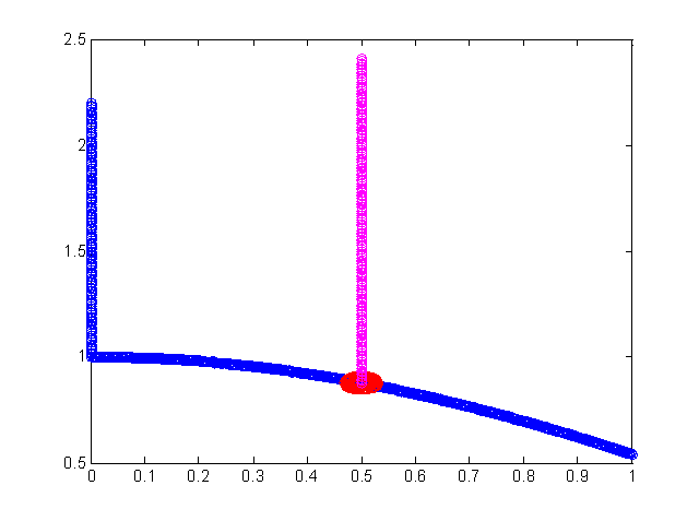
The boundary of the fundamental domain 𝒟 𝒟 \mathcal{D} 1
Γ a : : subscript Γ 𝑎 absent \displaystyle\Gamma_{a}: = { z ∈ ℍ : z = i y , y ≥ 1 } , Γ b := { z ∈ ℍ : z = e i θ , θ ∈ [ π 3 , π 2 ] } , formulae-sequence absent conditional-set 𝑧 ℍ formulae-sequence 𝑧 𝑖 𝑦 𝑦 1 assign subscript Γ 𝑏 conditional-set 𝑧 ℍ formulae-sequence 𝑧 superscript 𝑒 𝑖 𝜃 𝜃 𝜋 3 𝜋 2 \displaystyle=\{z\in\mathbb{H}:z=iy,\;y\geq 1\},\;\;\Gamma_{b}:=\{z\in\mathbb{H}:z=e^{i\theta},\;\theta\in[\frac{\pi}{3},\frac{\pi}{2}]\},
Γ c : : subscript Γ 𝑐 absent \displaystyle\Gamma_{c}: = { z ∈ ℍ : z = 1 2 + i y , y ≥ 3 2 } , ∂ 𝒟 = Γ a ∪ Γ b ∪ Γ c . formulae-sequence absent conditional-set 𝑧 ℍ formulae-sequence 𝑧 1 2 𝑖 𝑦 𝑦 3 2 𝒟 subscript Γ 𝑎 subscript Γ 𝑏 subscript Γ 𝑐 \displaystyle=\{z\in\mathbb{H}:z=\frac{1}{2}+iy,\;y\geq\frac{\sqrt{3}}{2}\},\;\;\partial\mathcal{D}=\Gamma_{a}\cup\Gamma_{b}\cup\Gamma_{c}.
Figure 1. Boundary of the fundamental domain 𝒟 𝒟 \mathcal{D}
The interior points of 𝒟 𝒟 \mathcal{D} 1.2 1.2 z ∈ Γ a 𝑧 subscript Γ 𝑎 z\in\Gamma_{a} z ∈ Γ b 𝑧 subscript Γ 𝑏 z\in\Gamma_{b} 1 2 − limit-from 1 2 \frac{1}{2}- z ∈ Γ c 𝑧 subscript Γ 𝑐 z\in\Gamma_{c} GL ( 2 , ℤ ) GL 2 ℤ \hbox{GL}(2,\mathbb{Z}) [7 ] .
In particular, the intersection point { i } = Γ a ∩ Γ b 𝑖 subscript Γ 𝑎 subscript Γ 𝑏 \{i\}=\Gamma_{a}\cap\Gamma_{b} { e i π 3 } = Γ b ∩ Γ c superscript 𝑒 𝑖 𝜋 3 subscript Γ 𝑏 subscript Γ 𝑐 \{e^{i\frac{\pi}{3}}\}=\Gamma_{b}\cap\Gamma_{c} i 𝑖 i e i π 3 superscript 𝑒 𝑖 𝜋 3 e^{i\frac{\pi}{3}} 𝐂 ~ ~ 𝐂 \tilde{\mathbf{C}} z 𝑧 z
Let L 𝐿 L 𝐰 1 , 𝐰 2 subscript 𝐰 1 subscript 𝐰 2
\mathbf{w}_{1},\mathbf{w}_{2} L 𝐿 L
z = 𝐰 2 𝐰 1 , or 𝐰 2 = z 𝐰 1 . formulae-sequence 𝑧 subscript 𝐰 2 subscript 𝐰 1 or subscript 𝐰 2 𝑧 subscript 𝐰 1 z=\frac{\mathbf{w}_{2}}{\mathbf{w}_{1}},\;\hbox{or}\;\;\mathbf{w}_{2}=z\mathbf{w}_{1}.
In this way, a Bravais lattice with unit density can be parameterized by L = 1 Im ( z ) ( ℤ ⊕ z ℤ ) 𝐿 1 Im 𝑧 direct-sum ℤ 𝑧 ℤ L=\sqrt{\frac{1}{\operatorname{Im}(z)}}\Big{(}{\mathbb{Z}}\oplus z{\mathbb{Z}}\Big{)} z ∈ ℍ 𝑧 ℍ z\in\mathbb{H}
A classical way to construct a strain energy density satisfying (1.3 J 𝐽 J [5 , 18 ] ), while a more general way is by the summation on the lattices through a external potential 𝐯 𝐯 \mathbf{v}
f ( z ) := ∑ ℙ ∈ L 𝐯 ( | ℙ | 2 ) . assign 𝑓 𝑧 subscript ℙ 𝐿 𝐯 superscript ℙ 2 \displaystyle f(z):=\sum_{\mathbb{P}\in L}\mathbf{v}(|\mathbb{P}|^{2}). (1.6)
It is straightforward to check that f ( z ) 𝑓 𝑧 f(z) 1.3 [11 ] proposed the lattice summation (1.6 1.6 1.6
This reformulation consisting in lattice summation form looks new and different, comparing the classical form of phase transitions consisting in integral form(see e.g. [8 , 16 ] and the references therein).
An interesting open question closely related to the Reformulation is
Problem A (Square-hexagonal phase transition, [7 , 6 ] , [7 ] Section 4, page 82).
Obtain a model energy for the square-hexagonal transformation, i.e., find a strain energy function( ( ( 1.3 ) ) )
•
( i ) 𝑖 (i) the square state is the global minimum and the hexagonal is unstable(precisely, a saddle point);
•
( i i ) 𝑖 𝑖 (ii) both the square and the hexagonal states are local minimum;
•
( i i i ) 𝑖 𝑖 𝑖 (iii) the hexagonal is the global minimum, and the square is unstable.
For phase transitions in crystals, Landau 1936([12 ] ) proposed a theory to explain it, namely, finding the minimum of the density function, further
this density function should has some symmetries. This theory was further developed by many mathematicians([10 , 11 , 7 , 6 , 18 ] etc.). In two dimensional crystals, these symmetries was further identified by SL ( 2 , ℤ ) SL 2 ℤ \hbox{SL}(2,\mathbb{Z})
A mathematical theory to explain hexagonal to square lattice phase transitions is to find a strain energy function with a parameter such that
its minimum is achieved at hexagonal lattice or square lattice as the parameter changing, without passing through the rhombic lattice.
This problem is initiated by Landau in 1936 and justified by many mathematicians and physicists.
Complex six-order polynomials were constructed to answer Problem A under the assumption that the reference lattice is either square or hexagonal([7 ] ), and recently in [5 , 2 , 3 ] , a modular invariant function
| J ( z ) − 1 | + α | J ( z ) | 2 / 3 , 𝐽 𝑧 1 𝛼 superscript 𝐽 𝑧 2 3 \displaystyle|J(z)-1|+\alpha|J(z)|^{2/3},
was constructed to answer Problem A by numerical computation restricted on the unit arc, where J 𝐽 J 1.1 1.6
Our idea is motivated from classical number theory, this is partially inspired by Parry [18 ] (page 2), where he remarked that”My purpose, here, is to describe and elaborate upon methods from classical complex analysis and number theory which have a natural application in this area( ( ( ) ) ) ”. In 1988, number theorist Montgomery [17 ] proved the following celebrated result:
Theorem A (Hexagonal lattice).
For all α > 0 𝛼 0 \alpha>0
min L ∑ ℙ ∈ L , | L | = 1 e − π α | ℙ | 2 is achieved at hexagonal lattice . subscript 𝐿 subscript formulae-sequence ℙ 𝐿 𝐿 1 superscript 𝑒 𝜋 𝛼 superscript ℙ 2 is achieved at hexagonal lattice \displaystyle\min_{L}\sum_{\mathbb{P}\in L,|L|=1}e^{-\pi\alpha|\mathbb{P}|^{2}}\;\;\hbox{is achieved at hexagonal lattice}. (1.8)
Here we fix the volume/density of the lattice to be 1 1 1 L = 2 3 ( ℤ ⊕ e i π 3 ℤ ) 𝐿 2 3 direct-sum ℤ superscript 𝑒 𝑖 𝜋 3 ℤ L=\sqrt{\frac{2}{\sqrt{3}}}\Big{(}{\mathbb{Z}}\oplus e^{i\frac{\pi}{3}}{\mathbb{Z}}\Big{)} [19 ] ).
Perhaps, the modular invariant function most related to ∑ ℙ ∈ L , | L | = 1 e − π α | ℙ | 2 subscript formulae-sequence ℙ 𝐿 𝐿 1 superscript 𝑒 𝜋 𝛼 superscript ℙ 2 \sum_{\mathbb{P}\in L,|L|=1}e^{-\pi\alpha|\mathbb{P}|^{2}} ∑ ℙ ∈ L , | L | = 1 | ℙ | 2 e − π α | ℙ | 2 subscript formulae-sequence ℙ 𝐿 𝐿 1 superscript ℙ 2 superscript 𝑒 𝜋 𝛼 superscript ℙ 2 \sum_{\mathbb{P}\in L,|L|=1}|\mathbb{P}|^{2}e^{-\pi\alpha|\mathbb{P}|^{2}} α 𝛼 \alpha
Theorem 1.1 (Hexagonal-Square-Rectangular Phase Transitions).
Assume that α > 0 𝛼 0 \alpha>0 α a < α b ∈ ( 4 5 , 1 ) subscript 𝛼 𝑎 subscript 𝛼 𝑏 4 5 1 \alpha_{a}<\alpha_{b}\in(\frac{4}{5},1)
min L ∑ ℙ ∈ L , | L | = 1 | ℙ | 2 e − π α | ℙ | 2 is achieved at { r e c t a n g u l a r l a t t i c e , if α ∈ ( 0 , α a ) , s q u a r e l a t t i c e if α ∈ [ α a , α b ) , s q u a r e or h e x a g o n a l l a t t i c e if α = α b , h e x a g o n a l l a t t i c e , if α ∈ ( α b , ∞ ) . subscript 𝐿 subscript formulae-sequence ℙ 𝐿 𝐿 1 superscript ℙ 2 superscript 𝑒 𝜋 𝛼 superscript ℙ 2 is achieved at cases 𝑟 𝑒 𝑐 𝑡 𝑎 𝑛 𝑔 𝑢 𝑙 𝑎 𝑟 𝑙 𝑎 𝑡 𝑡 𝑖 𝑐 𝑒 if 𝛼 0 subscript 𝛼 𝑎 𝑠 𝑞 𝑢 𝑎 𝑟 𝑒 𝑙 𝑎 𝑡 𝑡 𝑖 𝑐 𝑒 if 𝛼 subscript 𝛼 𝑎 subscript 𝛼 𝑏 𝑠 𝑞 𝑢 𝑎 𝑟 𝑒 or ℎ 𝑒 𝑥 𝑎 𝑔 𝑜 𝑛 𝑎 𝑙 𝑙 𝑎 𝑡 𝑡 𝑖 𝑐 𝑒 if 𝛼 subscript 𝛼 𝑏 ℎ 𝑒 𝑥 𝑎 𝑔 𝑜 𝑛 𝑎 𝑙 𝑙 𝑎 𝑡 𝑡 𝑖 𝑐 𝑒 if 𝛼 subscript 𝛼 𝑏 \displaystyle\min_{L}\sum_{\mathbb{P}\in L,|L|=1}|\mathbb{P}|^{2}e^{-\pi\alpha|\mathbb{P}|^{2}}\;\;\hbox{is achieved at}\;\;\begin{cases}\;\;rectangular\;lattice,&\hbox{if}\;\;\alpha\in(0,\alpha_{a}),\\
\;\;square\;lattice\;&\hbox{if}\;\;\alpha\in[\alpha_{a},\alpha_{b}),\\
\;\;square\;\hbox{or}\;hexagonal\;lattice&\hbox{if}\;\;\alpha=\alpha_{b},\\
\;\;hexagonal\;lattice,&\hbox{if}\;\;\alpha\in(\alpha_{b},\infty).\end{cases}
Here, numerically,
α a := 0.8947042694 ⋯ , α b := 0.9203340927 ⋯ . formulae-sequence assign subscript 𝛼 𝑎 0.8947042694 ⋯ assign subscript 𝛼 𝑏 0.9203340927 ⋯ \displaystyle\alpha_{a}:=0.8947042694\cdots,\;\;\alpha_{b}:=0.9203340927\cdots.
A square lattice can be parameterized by L = ( ℤ ⊕ i ℤ ) 𝐿 direct-sum ℤ 𝑖 ℤ L=\Big{(}{\mathbb{Z}}\oplus i{\mathbb{Z}}\Big{)} L = 1 y ( ℤ ⊕ i y ℤ ) 𝐿 1 𝑦 direct-sum ℤ 𝑖 𝑦 ℤ L=\sqrt{\frac{1}{y}}\Big{(}{\mathbb{Z}}\oplus iy{\mathbb{Z}}\Big{)} y > 1 𝑦 1 y>1 1.1
Problem A is answered by the following result (after reordering and re-scaling the parameter, e.g. α ↦ 1 α , α ↦ k ⋅ α formulae-sequence maps-to 𝛼 1 𝛼 maps-to 𝛼 ⋅ 𝑘 𝛼 \alpha\mapsto\frac{1}{\alpha},\alpha\mapsto k\cdot\alpha 1.1 α 𝛼 \alpha 1 α 1 𝛼 \frac{1}{\alpha} α a , α b subscript 𝛼 𝑎 subscript 𝛼 𝑏
\alpha_{a},\alpha_{b} 0 o , 100 o superscript 0 𝑜 superscript 100 𝑜
0^{o},100^{o}
Corollary 1.1 (Hexagonal-Square Phase Transitions).
Assume that α ≥ α a 𝛼 subscript 𝛼 𝑎 \alpha\geq\alpha_{a}
min L ∑ ℙ ∈ L , | L | = 1 | ℙ | 2 e − π α | ℙ | 2 is achieved at { s q u a r e l a t t i c e if α ∈ [ α a , α b ) , s q u a r e or h e x a g o n a l l a t t i c e if α = α b , h e x a g o n a l l a t t i c e , if α ∈ ( α b , ∞ ) . subscript 𝐿 subscript formulae-sequence ℙ 𝐿 𝐿 1 superscript ℙ 2 superscript 𝑒 𝜋 𝛼 superscript ℙ 2 is achieved at cases 𝑠 𝑞 𝑢 𝑎 𝑟 𝑒 𝑙 𝑎 𝑡 𝑡 𝑖 𝑐 𝑒 if 𝛼 subscript 𝛼 𝑎 subscript 𝛼 𝑏 𝑠 𝑞 𝑢 𝑎 𝑟 𝑒 or ℎ 𝑒 𝑥 𝑎 𝑔 𝑜 𝑛 𝑎 𝑙 𝑙 𝑎 𝑡 𝑡 𝑖 𝑐 𝑒 if 𝛼 subscript 𝛼 𝑏 ℎ 𝑒 𝑥 𝑎 𝑔 𝑜 𝑛 𝑎 𝑙 𝑙 𝑎 𝑡 𝑡 𝑖 𝑐 𝑒 if 𝛼 subscript 𝛼 𝑏 \displaystyle\min_{L}\sum_{\mathbb{P}\in L,|L|=1}|\mathbb{P}|^{2}e^{-\pi\alpha|\mathbb{P}|^{2}}\;\;\hbox{is achieved at}\;\;\begin{cases}\;\;square\;lattice\;&\hbox{if}\;\;\alpha\in[\alpha_{a},\alpha_{b}),\\
\;\;square\;\hbox{or}\;hexagonal\;lattice&\hbox{if}\;\;\alpha=\alpha_{b},\\
\;\;hexagonal\;lattice,&\hbox{if}\;\;\alpha\in(\alpha_{b},\infty).\end{cases}
Here, numerically,
α a := 0.8947042694 ⋯ , α b := 0.9203340927 ⋯ . formulae-sequence assign subscript 𝛼 𝑎 0.8947042694 ⋯ assign subscript 𝛼 𝑏 0.9203340927 ⋯ \displaystyle\alpha_{a}:=0.8947042694\cdots,\;\;\alpha_{b}:=0.9203340927\cdots.
Via the classification and representation of 2d lattices in [7 ] , we have
Corollary 1.2 (Minimization on the Cauchy-Green tensor).
Assume that α ≥ α a 𝛼 subscript 𝛼 𝑎 \alpha\geq\alpha_{a}
min 𝐂 > 0 , 𝐂 T = 𝐂 ∑ ( m , n ) ∈ ℤ 2 e − π α 𝐂 11 𝐂 11 𝐂 22 − 𝐂 12 2 | m 𝐂 12 + 𝐂 11 C 22 − 𝐂 12 2 ⋅ i 𝐂 11 + n | 2 subscript formulae-sequence 𝐂 0 superscript 𝐂 𝑇 𝐂 subscript 𝑚 𝑛 superscript ℤ 2 superscript 𝑒 𝜋 𝛼 subscript 𝐂 11 subscript 𝐂 11 subscript 𝐂 22 superscript subscript 𝐂 12 2 superscript 𝑚 subscript 𝐂 12 ⋅ subscript 𝐂 11 subscript 𝐶 22 superscript subscript 𝐂 12 2 𝑖 subscript 𝐂 11 𝑛 2 \displaystyle\min_{\mathbf{C}>0,\mathbf{C}^{T}=\mathbf{C}}\sum_{(m,n)\in\mathbb{Z}^{2}}e^{-\pi\alpha\frac{\mathbf{C}_{11}}{\sqrt{\mathbf{C}_{11}\mathbf{C}_{22}-\mathbf{C}_{12}^{2}}}|m\frac{\mathbf{C}_{12}+\sqrt{\mathbf{C}_{11}C_{22}-\mathbf{C}_{12}^{2}}\cdot i}{\mathbf{C}_{11}}+n|^{2}}\;\;
is achieved at { 𝐂 11 = 𝐂 22 = 2 𝐂 12 > 0 , if α ∈ [ α a , α b ] , 𝐂 11 = 𝐂 22 > 0 , 𝐂 12 = 0 , if α ∈ [ α b , ∞ ) . cases subscript 𝐂 11 subscript 𝐂 22 2 subscript 𝐂 12 0 if 𝛼 subscript 𝛼 𝑎 subscript 𝛼 𝑏 formulae-sequence subscript 𝐂 11 subscript 𝐂 22 0 subscript 𝐂 12 0 if 𝛼 subscript 𝛼 𝑏 \displaystyle\begin{cases}\;\;\mathbf{C}_{11}=\mathbf{C}_{22}=2\mathbf{C}_{12}>0,&\hbox{if}\;\;\alpha\in[\alpha_{a},\alpha_{b}],\\
\;\;\mathbf{C}_{11}=\mathbf{C}_{22}>0,\mathbf{C}_{12}=0,&\hbox{if}\;\;\alpha\in[\alpha_{b},\infty).\end{cases}
Here, numerically,
α a := 0.8947042694 ⋯ , α b := 0.9203340927 ⋯ . formulae-sequence assign subscript 𝛼 𝑎 0.8947042694 ⋯ assign subscript 𝛼 𝑏 0.9203340927 ⋯ \displaystyle\alpha_{a}:=0.8947042694\cdots,\;\;\alpha_{b}:=0.9203340927\cdots.
By Corollary 1.1 Problem A is ∑ ℙ ∈ L , | L | = 1 | ℙ | 2 e − π α | ℙ | 2 subscript formulae-sequence ℙ 𝐿 𝐿 1 superscript ℙ 2 superscript 𝑒 𝜋 𝛼 superscript ℙ 2 \sum_{\mathbb{P}\in L,|L|=1}|\mathbb{P}|^{2}e^{-\pi\alpha|\mathbb{P}|^{2}} α ≥ α a 𝛼 subscript 𝛼 𝑎 \alpha\geq\alpha_{a} 1.9 Problem A .
By the parametrization of the Bravais lattice with fixed density ρ 𝜌 \rho ρ > 0 𝜌 0 \rho>0
∑ ℙ ∈ L , | L | = ρ | ℙ | 2 e − π α | ℙ | 2 = ∑ ( m , n ) ∈ ℤ 2 | m z + n | 2 Im ( z ) e − π ⋅ α ⋅ ρ | m z + n | 2 Im ( z ) . subscript formulae-sequence ℙ 𝐿 𝐿 𝜌 superscript ℙ 2 superscript 𝑒 𝜋 𝛼 superscript ℙ 2 subscript 𝑚 𝑛 superscript ℤ 2 superscript 𝑚 𝑧 𝑛 2 Im 𝑧 superscript 𝑒 ⋅ 𝜋 𝛼 𝜌 superscript 𝑚 𝑧 𝑛 2 Im 𝑧 \displaystyle\sum_{\mathbb{P}\in L,|L|=\rho}|\mathbb{P}|^{2}e^{-\pi\alpha|\mathbb{P}|^{2}}=\sum_{(m,n)\in\mathbb{Z}^{2}}\frac{|mz+n|^{2}}{\operatorname{Im}(z)}e^{-\frac{\pi\cdot\alpha\cdot\rho|mz+n|^{2}}{\operatorname{Im}(z)}}. (1.10)
By the parametrization, with loss of generality, we assume that density the lattice is 1 in statement of previous theorems.
The proof of Theorem 1.1
Theorem 1.2 (Minimization).
For all α > 0 𝛼 0 \alpha>0
min z ∈ ℍ ∑ ( m , n ) ∈ ℤ 2 | m z + n | 2 Im ( z ) e − π α | m z + n | 2 Im ( z ) is achieved at { i y α , if α ∈ ( 0 , α a ) , i if α ∈ [ α a , α b ) , i or e i π 3 if α = α b , e i π 3 , if α ∈ ( α b , ∞ ) . subscript 𝑧 ℍ subscript 𝑚 𝑛 superscript ℤ 2 superscript 𝑚 𝑧 𝑛 2 Im 𝑧 superscript 𝑒 𝜋 𝛼 superscript 𝑚 𝑧 𝑛 2 Im 𝑧 is achieved at cases 𝑖 subscript 𝑦 𝛼 if 𝛼 0 subscript 𝛼 𝑎 𝑖 if 𝛼 subscript 𝛼 𝑎 subscript 𝛼 𝑏 𝑖 or superscript 𝑒 𝑖 𝜋 3 if 𝛼 subscript 𝛼 𝑏 superscript 𝑒 𝑖 𝜋 3 if 𝛼 subscript 𝛼 𝑏 \displaystyle\min_{z\in\mathbb{H}}\sum_{(m,n)\in\mathbb{Z}^{2}}\frac{|mz+n|^{2}}{\operatorname{Im}(z)}e^{-\frac{\pi\alpha|mz+n|^{2}}{\operatorname{Im}(z)}}\;\;\hbox{is achieved at}\;\;\begin{cases}\;\;iy_{\alpha},&\hbox{if}\;\;\alpha\in(0,\alpha_{a}),\\
\;\;i\;&\hbox{if}\;\;\alpha\in[\alpha_{a},\alpha_{b}),\\
\;\;i\;\hbox{or}\;e^{i\frac{\pi}{3}}&\hbox{if}\;\;\alpha=\alpha_{b},\\
\;\;e^{i\frac{\pi}{3}},&\hbox{if}\;\;\alpha\in(\alpha_{b},\infty).\end{cases} (1.11)
Here, numerically,
α a := 0.8947042694 ⋯ , α b := 0.9203340927 ⋯ , formulae-sequence assign subscript 𝛼 𝑎 0.8947042694 ⋯ assign subscript 𝛼 𝑏 0.9203340927 ⋯ \displaystyle\alpha_{a}:=0.8947042694\cdots,\;\;\alpha_{b}:=0.9203340927\cdots,
and y α > 1 subscript 𝑦 𝛼 1 y_{\alpha}>1 y α subscript 𝑦 𝛼 y_{\alpha} α 𝛼 \alpha
d y α d α < 0 . 𝑑 subscript 𝑦 𝛼 𝑑 𝛼 0 \frac{dy_{\alpha}}{d\alpha}<0.
Let
M ( α , z ) = ∑ ( m , n ) ∈ ℤ 2 | m z + n | 2 Im ( z ) e − π α | m z + n | 2 Im ( z ) , θ ( α , z ) = ∑ ( m , n ) ∈ ℤ 2 e − π α | m z + n | 2 Im ( z ) formulae-sequence 𝑀 𝛼 𝑧 subscript 𝑚 𝑛 superscript ℤ 2 superscript 𝑚 𝑧 𝑛 2 Im 𝑧 superscript 𝑒 𝜋 𝛼 superscript 𝑚 𝑧 𝑛 2 Im 𝑧 𝜃 𝛼 𝑧 subscript 𝑚 𝑛 superscript ℤ 2 superscript 𝑒 𝜋 𝛼 superscript 𝑚 𝑧 𝑛 2 Im 𝑧 \displaystyle{M}(\alpha,z)=\sum_{(m,n)\in\mathbb{Z}^{2}}\frac{|mz+n|^{2}}{\operatorname{Im}(z)}e^{-\pi\alpha\frac{|mz+n|^{2}}{\operatorname{Im}(z)}},\;\;\theta(\alpha,z)=\sum_{(m,n)\in\mathbb{Z}^{2}}e^{-\pi\alpha\frac{|mz+n|^{2}}{\operatorname{Im}(z)}}
then analytically,
α b subscript 𝛼 𝑏 \alpha_{b}
M ( α , i ) = M ( α , e i π 3 ) , for α ∈ [ 5 6 , 1 ] , formulae-sequence 𝑀 𝛼 𝑖 𝑀 𝛼 superscript 𝑒 𝑖 𝜋 3 for 𝛼 5 6 1 M(\alpha,i)=M(\alpha,e^{i\frac{\pi}{3}}),\;\;\hbox{for}\;\;\alpha\in[\frac{5}{6},1],
1 α a 1 subscript 𝛼 𝑎 \frac{1}{\alpha_{a}} is the unique solution of
θ y y ( α , i ) = π α M y y ( α , i ) , for α ∈ [ 1 , 9 8 ] . formulae-sequence subscript 𝜃 𝑦 𝑦 𝛼 𝑖 𝜋 𝛼 subscript 𝑀 𝑦 𝑦 𝛼 𝑖 for 𝛼 1 9 8 \displaystyle\theta_{yy}(\alpha,i)=\pi\alpha M_{yy}(\alpha,i),\;\;\hbox{for}\;\;\alpha\in[1,\frac{9}{8}].
The y α subscript 𝑦 𝛼 y_{\alpha} 1.2 α 𝛼 \alpha
Table 1 .
An illustration of Theorem 1.1 1 1.1
We provide more examples to admit the hexagonal to square phase transitions(answering Problem A ).
Theorem 1.3 (Hexagonal-Square Phase Transitions).
Assume that α > 0 𝛼 0 \alpha>0 γ > 0 𝛾 0 \gamma>0 α γ 1 < α γ 2 ∈ ( 0 , 1 ) subscript 𝛼 subscript 𝛾 1 subscript 𝛼 subscript 𝛾 2 0 1 \alpha_{\gamma_{1}}<\alpha_{\gamma_{2}}\in(0,1)
min L ∑ ℙ ∈ L , | L | = 1 ( | ℙ | 2 + γ ) e − π α | ℙ | 2 is achieved at { s q u a r e l a t t i c e if α ∈ [ α γ 1 , α γ 2 ) , s q u a r e or h e x a g o n a l l a t t i c e if α = α γ 2 , h e x a g o n a l l a t t i c e , if α ∈ ( α γ 2 , ∞ ) . subscript 𝐿 subscript formulae-sequence ℙ 𝐿 𝐿 1 superscript ℙ 2 𝛾 superscript 𝑒 𝜋 𝛼 superscript ℙ 2 is achieved at cases 𝑠 𝑞 𝑢 𝑎 𝑟 𝑒 𝑙 𝑎 𝑡 𝑡 𝑖 𝑐 𝑒 if 𝛼 subscript 𝛼 subscript 𝛾 1 subscript 𝛼 subscript 𝛾 2 𝑠 𝑞 𝑢 𝑎 𝑟 𝑒 or ℎ 𝑒 𝑥 𝑎 𝑔 𝑜 𝑛 𝑎 𝑙 𝑙 𝑎 𝑡 𝑡 𝑖 𝑐 𝑒 if 𝛼 subscript 𝛼 subscript 𝛾 2 ℎ 𝑒 𝑥 𝑎 𝑔 𝑜 𝑛 𝑎 𝑙 𝑙 𝑎 𝑡 𝑡 𝑖 𝑐 𝑒 if 𝛼 subscript 𝛼 subscript 𝛾 2 \displaystyle\min_{L}\sum_{\mathbb{P}\in L,|L|=1}(|\mathbb{P}|^{2}+\gamma)e^{-\pi\alpha|\mathbb{P}|^{2}}\;\;\hbox{is achieved at}\;\;\begin{cases}\;\;square\;lattice\;&\hbox{if}\;\;\alpha\in[\alpha_{\gamma_{1}},\alpha_{\gamma_{2}}),\\
\;\;square\;\hbox{or}\;hexagonal\;lattice&\hbox{if}\;\;\alpha=\alpha_{\gamma_{2}},\\
\;\;hexagonal\;lattice,&\hbox{if}\;\;\alpha\in(\alpha_{\gamma_{2}},\infty).\end{cases}
Some comments are in order. We obtain several classes of modular invariant functions admitting
hexagonal to square phase transitions. This is the first time to obtain such functions, although it was
conjectured to exist for long time. On the other hand, continuous hexagonal-rhombic-square-rectangular phase transitions have been observed and rigorously established in many modular invariant functions. See [13 , 14 ] .
Given by Theorems 1.1 1.3
∑ ℙ ∈ L , | L | = 1 | ℙ | 4 e − π α | ℙ | 2 , subscript formulae-sequence ℙ 𝐿 𝐿 1 superscript ℙ 4 superscript 𝑒 𝜋 𝛼 superscript ℙ 2 \sum_{\mathbb{P}\in L,|L|=1}|\mathbb{P}|^{4}e^{-\pi\alpha|\mathbb{P}|^{2}},
however this is not true (by numerically computations).
Hexagonal and square lattices have the dominated role in two dimensional Bravais lattices (as seen in Theorem 1.1 1.1
Open Problem 1.1 .
Classify
min L ∑ ℙ ∈ L , | L | = 1 | ℙ | 2 e − π α | ℙ | 2 , here L is a 3-dimensional lattice and α > 0 . subscript 𝐿 subscript formulae-sequence ℙ 𝐿 𝐿 1 superscript ℙ 2 superscript 𝑒 𝜋 𝛼 superscript ℙ 2 here 𝐿 is a 3-dimensional lattice and 𝛼
0 \displaystyle\min_{L}\sum_{\mathbb{P}\in L,|L|=1}|\mathbb{P}|^{2}e^{-\pi\alpha|\mathbb{P}|^{2}},\;\;\hbox{here}\;\;L\;\;\hbox{is a 3-dimensional lattice and}\;\;\alpha>0.
The paper is organized as follows: in Section 2, we collect some basic properties of the functionals and some basic estimates of derivatives of Jacobi theta functions.
In Section 3, we prove a transversal monotonicity of the functionals, as a consequence, we show that for certain range of α 𝛼 \alpha Γ a ∪ Γ b subscript Γ 𝑎 subscript Γ 𝑏 \Gamma_{a}\cup\Gamma_{b} 1
In Section 4, we establish a minimum principle of modular invariant functions and deduce several second-order estimates in using the minimum principle, as a consequence, we prove that for certain range of α 𝛼 \alpha Γ b subscript Γ 𝑏 \Gamma_{b} 1
By the main results in Sections 3 and 4, we obtain that for the full range of α ( α > 0 ) 𝛼 𝛼 0 \alpha(\alpha>0) Γ a ∪ Γ b subscript Γ 𝑎 subscript Γ 𝑏 \Gamma_{a}\cup\Gamma_{b} 1
In Sections 5 and 6, we develop effective methods to analyze the functionals on the vertical line Γ a subscript Γ 𝑎 \Gamma_{a} 1 4 − limit-from 1 4 \frac{1}{4}- Γ b subscript Γ 𝑏 \Gamma_{b} 1
Finally, we give the proof of our main Theorem in Section 7.
3. The transversal monotonicity
Recall that the lattice with unit density is parameterized by L = 1 Im ( z ) ( ℤ ⊕ z ℤ ) 𝐿 1 Im 𝑧 direct-sum ℤ 𝑧 ℤ L=\sqrt{\frac{1}{\operatorname{Im}(z)}}\Big{(}{\mathbb{Z}}\oplus z{\mathbb{Z}}\Big{)}
θ ( α , z ) : : 𝜃 𝛼 𝑧 absent \displaystyle\theta(\alpha,z): = ∑ ℙ ∈ L , | L | = 1 e − π α | ℙ | 2 = ∑ ( m , n ) ∈ ℤ 2 e − π α 1 Im ( z ) | m z + n | 2 . absent subscript formulae-sequence ℙ 𝐿 𝐿 1 superscript 𝑒 𝜋 𝛼 superscript ℙ 2 subscript 𝑚 𝑛 superscript ℤ 2 superscript 𝑒 𝜋 𝛼 1 Im 𝑧 superscript 𝑚 𝑧 𝑛 2 \displaystyle=\sum_{\mathbb{P}\in L,\;|L|=1}e^{-\pi\alpha|\mathbb{P}|^{2}}=\sum_{(m,n)\in\mathbb{Z}^{2}}e^{-\pi\alpha\frac{1}{\operatorname{Im}(z)}|mz+n|^{2}}. (3.8)
We then define the M 𝑀 {M}
M ( α , z ) : : 𝑀 𝛼 𝑧 absent \displaystyle{M}(\alpha,z): = ∑ ℙ ∈ L , | L | = 1 | ℙ | 2 e − π α | ℙ | 2 = ∑ ( m , n ) ∈ ℤ 2 | m z + n | 2 Im ( z ) e − π α | m z + n | 2 Im ( z ) . absent subscript formulae-sequence ℙ 𝐿 𝐿 1 superscript ℙ 2 superscript 𝑒 𝜋 𝛼 superscript ℙ 2 subscript 𝑚 𝑛 superscript ℤ 2 superscript 𝑚 𝑧 𝑛 2 Im 𝑧 superscript 𝑒 𝜋 𝛼 superscript 𝑚 𝑧 𝑛 2 Im 𝑧 \displaystyle=\sum_{\mathbb{P}\in L,\;|L|=1}|\mathbb{P}|^{2}e^{-\pi\alpha|\mathbb{P}|^{2}}=\sum_{(m,n)\in\mathbb{Z}^{2}}\frac{|mz+n|^{2}}{\operatorname{Im}(z)}e^{-\pi\alpha\frac{|mz+n|^{2}}{\operatorname{Im}(z)}}. (3.9)
We also recall that right-half fundamental domain
𝒟 𝒢 := { z ∈ ℍ : | z | > 1 , 0 < x < 1 2 } . assign subscript 𝒟 𝒢 conditional-set 𝑧 ℍ formulae-sequence 𝑧 1 0 𝑥 1 2 \displaystyle\mathcal{D}_{\mathcal{G}}:=\{z\in\mathbb{H}:|z|>1,\;0<x<\frac{1}{2}\}.
The boundaries of 𝒟 𝒢 subscript 𝒟 𝒢 \mathcal{D}_{\mathcal{G}}
Γ a : : subscript Γ 𝑎 absent \displaystyle\Gamma_{a}: = { z ∈ ℍ : z = i y , y ≥ 1 } , absent conditional-set 𝑧 ℍ formulae-sequence 𝑧 𝑖 𝑦 𝑦 1 \displaystyle=\{z\in\mathbb{H}:z=iy,\;y\geq 1\},
Γ b : : subscript Γ 𝑏 absent \displaystyle\Gamma_{b}: = { z ∈ ℍ : z = e i θ , θ ∈ [ π 3 , π 2 ] } , absent conditional-set 𝑧 ℍ formulae-sequence 𝑧 superscript 𝑒 𝑖 𝜃 𝜃 𝜋 3 𝜋 2 \displaystyle=\{z\in\mathbb{H}:z=e^{i\theta},\;\theta\in[\frac{\pi}{3},\frac{\pi}{2}]\},
Γ = Γ a ∪ Γ b . Γ subscript Γ 𝑎 subscript Γ 𝑏 \displaystyle\Gamma=\Gamma_{a}\cup\Gamma_{b}.
In [15 ] , we already prove that
min z ∈ ℍ M ( α , z ) is achieved at e i π 3 for α ≥ 1 . subscript 𝑧 ℍ 𝑀 𝛼 𝑧 is achieved at superscript 𝑒 𝑖 𝜋 3 for 𝛼 1 \displaystyle\min_{z\in\mathbb{H}}M(\alpha,z)\;\;\hbox{is achieved at}\;\;e^{i\frac{\pi}{3}}\;\;\hbox{for}\;\;\alpha\geq 1.
In this Section, we aim to prove that
Proposition 3.1 .
For α ∈ ( 0 , 0.9155730607 ) 𝛼 0 0.9155730607 \alpha\in(0,0.9155730607)
min z ∈ ℍ M ( α , z ) = min z ∈ 𝒟 𝒢 ¯ M ( α , z ) = min z ∈ Γ M ( α , z ) . subscript 𝑧 ℍ 𝑀 𝛼 𝑧 subscript 𝑧 ¯ subscript 𝒟 𝒢 𝑀 𝛼 𝑧 subscript 𝑧 Γ 𝑀 𝛼 𝑧 \displaystyle\min_{z\in\mathbb{H}}M(\alpha,z)=\min_{z\in\overline{\mathcal{D}_{\mathcal{G}}}}M(\alpha,z)=\min_{z\in\Gamma}M(\alpha,z).
The proof of Proposition 3.1
Proposition 3.2 .
For α ∈ ( 0 , 0.9155730607 ) 𝛼 0 0.9155730607 \alpha\in(0,0.9155730607)
∂ ∂ x M ( α , z ) > 0 , for z ∈ 𝒟 𝒢 . formulae-sequence 𝑥 𝑀 𝛼 𝑧 0 for 𝑧 subscript 𝒟 𝒢 \displaystyle\frac{\partial}{\partial x}M(\alpha,z)>0,\;\;\hbox{for}\;\;z\in\mathcal{D}_{\mathcal{G}}.
We first state a useful lemma.
Lemma 3.1 (Duality of M 𝑀 M 1 α 1 𝛼 \frac{1}{\alpha} α 𝛼 \alpha .
Assume that α > 0 𝛼 0 \alpha>0
M ( 1 α , z ) = α 2 π ( θ ( α , z ) − π α M ( α , z ) ) . 𝑀 1 𝛼 𝑧 superscript 𝛼 2 𝜋 𝜃 𝛼 𝑧 𝜋 𝛼 𝑀 𝛼 𝑧 \displaystyle M(\frac{1}{\alpha},z)=\frac{\alpha^{2}}{\pi}\Big{(}\theta(\alpha,z)-\pi\alpha M(\alpha,z)\Big{)}.
Proof.
By Fourier transform,
θ ( 1 α , z ) = α θ ( α , z ) . 𝜃 1 𝛼 𝑧 𝛼 𝜃 𝛼 𝑧 \displaystyle\theta(\frac{1}{\alpha},z)=\alpha\theta(\alpha,z). (3.10)
Taking derivative with respect to α 𝛼 \alpha 3.10
− 1 α 2 ∂ ∂ α θ ( 1 α , z ) = θ ( α , z ) + α ∂ ∂ α θ ( α , z ) . 1 superscript 𝛼 2 𝛼 𝜃 1 𝛼 𝑧 𝜃 𝛼 𝑧 𝛼 𝛼 𝜃 𝛼 𝑧 \displaystyle-\frac{1}{\alpha^{2}}\frac{\partial}{\partial\alpha}\theta(\frac{1}{\alpha},z)=\theta(\alpha,z)+\alpha\frac{\partial}{\partial\alpha}\theta(\alpha,z). (3.11)
The result then follows by (3.11 3.2
The new function M 𝑀 M
Lemma 3.2 (A relation between the functions M 𝑀 M θ 𝜃 \theta .
M ( α , z ) = − 1 π ∂ ∂ α θ ( α , z ) . 𝑀 𝛼 𝑧 1 𝜋 𝛼 𝜃 𝛼 𝑧 \displaystyle M(\alpha,z)=-\frac{1}{\pi}\frac{\partial}{\partial\alpha}\theta(\alpha,z).
Proof.
It is based an cute observation from (3.8 3.9
By Lemma 3.1 3.2
Proposition 3.3 .
For α ∈ ( 1.092212127 , ∞ ) 𝛼 1.092212127 \alpha\in(1.092212127,\infty)
∂ ∂ x ( θ ( α , z ) − π α M ( α , z ) ) > 0 , for z ∈ 𝒟 𝒢 . formulae-sequence 𝑥 𝜃 𝛼 𝑧 𝜋 𝛼 𝑀 𝛼 𝑧 0 for 𝑧 subscript 𝒟 𝒢 \displaystyle\frac{\partial}{\partial x}\Big{(}\theta(\alpha,z)-\pi\alpha M(\alpha,z)\Big{)}>0,\;\;\hbox{for}\;\;z\in\mathcal{D}_{\mathcal{G}}.
In the rest of this section, we give the proof of Proposition 3.3 3.3
By the explicit expression of θ 𝜃 \theta 3.8 θ 𝜃 \theta 2.5 2.6
Lemma 3.3 (Reduction of dimension).
It holds that
θ ( α , z ) 𝜃 𝛼 𝑧 \displaystyle\theta(\alpha,z) = y α ∑ n ∈ ℤ e − π α y n 2 ϑ ( y α ; n x ) absent 𝑦 𝛼 subscript 𝑛 ℤ superscript 𝑒 𝜋 𝛼 𝑦 superscript 𝑛 2 italic-ϑ 𝑦 𝛼 𝑛 𝑥
\displaystyle=\sqrt{\frac{y}{\alpha}}\sum_{n\in\mathbb{Z}}e^{-\pi\alpha yn^{2}}\vartheta(\frac{y}{\alpha};nx)
∂ ∂ x θ ( α , z ) 𝑥 𝜃 𝛼 𝑧 \displaystyle\frac{\partial}{\partial x}\theta(\alpha,z) = 2 y α ∑ n = 1 ∞ n e − π α y n 2 ϑ Y ( y α ; n x ) . absent 2 𝑦 𝛼 superscript subscript 𝑛 1 𝑛 superscript 𝑒 𝜋 𝛼 𝑦 superscript 𝑛 2 subscript italic-ϑ 𝑌 𝑦 𝛼 𝑛 𝑥
\displaystyle=2\sqrt{\frac{y}{\alpha}}\sum_{n=1}^{\infty}ne^{-\pi\alpha yn^{2}}\vartheta_{Y}(\frac{y}{\alpha};nx).
By Lemmas 3.2 3.3
Lemma 3.4 (An exponentially decaying expansion of ∂ ∂ x M ( α , z ) 𝑥 𝑀 𝛼 𝑧 \frac{\partial}{\partial x}M(\alpha,z) .
∂ ∂ x M ( α , z ) 𝑥 𝑀 𝛼 𝑧 \displaystyle\frac{\partial}{\partial x}M(\alpha,z) = 1 π ( y α − 3 2 ∑ n = 1 ∞ n e − π α y n 2 ϑ Y ( y α ; n x ) + 2 π y 3 2 α − 1 2 ∑ n = 1 ∞ n 3 e − π α y n 2 ϑ Y ( y α ; n x ) \displaystyle=\frac{1}{\pi}\Big{(}\sqrt{y}\alpha^{-\frac{3}{2}}\sum_{n=1}^{\infty}ne^{-\pi\alpha yn^{2}}\vartheta_{Y}(\frac{y}{\alpha};nx)+2\pi y^{\frac{3}{2}}\alpha^{-\frac{1}{2}}\sum_{n=1}^{\infty}n^{3}e^{-\pi\alpha yn^{2}}\vartheta_{Y}(\frac{y}{\alpha};nx)
+ 2 y 3 2 α − 5 2 ∑ n = 1 ∞ n e − π α y n 2 ϑ X Y ( y α ; n x ) ) . \displaystyle\;\;\;\;+2y^{\frac{3}{2}}\alpha^{-\frac{5}{2}}\sum_{n=1}^{\infty}ne^{-\pi\alpha yn^{2}}\vartheta_{XY}(\frac{y}{\alpha};nx)\Big{)}.
Lemma 3.5 (An exponentially decaying expansion of ∂ ∂ x ( θ ( α , z ) − π α M ( α , z ) ) 𝑥 𝜃 𝛼 𝑧 𝜋 𝛼 𝑀 𝛼 𝑧 \frac{\partial}{\partial x}\Big{(}\theta(\alpha,z)-\pi\alpha M(\alpha,z)\Big{)} .
∂ ∂ x ( θ ( α , z ) − π α M ( α , z ) ) = 𝑥 𝜃 𝛼 𝑧 𝜋 𝛼 𝑀 𝛼 𝑧 absent \displaystyle\frac{\partial}{\partial x}\Big{(}\theta(\alpha,z)-\pi\alpha M(\alpha,z)\Big{)}= y α − 3 2 ⋅ ( − ϑ Y ( y α ; x ) ) ⋅ e − π α y ( 2 π y α 2 ∑ n = 1 ∞ n 3 e − π α y ( n 2 − 1 ) ϑ Y ( y α ; n x ) ϑ Y ( y α ; x ) \displaystyle\sqrt{y}\alpha^{-\frac{3}{2}}\cdot(-\vartheta_{Y}(\frac{y}{\alpha};x))\cdot e^{-\pi\alpha y}\Big{(}2\pi y\alpha^{2}\sum_{n=1}^{\infty}n^{3}e^{-\pi\alpha y(n^{2}-1)}\frac{\vartheta_{Y}(\frac{y}{\alpha};nx)}{\vartheta_{Y}(\frac{y}{\alpha};x)}
− 2 y ∑ n = 1 ∞ n e − π α y ( n 2 − 1 ) ϑ X Y ( y α ; n x ) − ϑ Y ( y α ; x ) − α ∑ n = 1 ∞ n e − π α y ( n 2 − 1 ) ϑ Y ( y α ; n x ) ϑ Y ( y α ; x ) ) \displaystyle-2y\sum_{n=1}^{\infty}ne^{-\pi\alpha y(n^{2}-1)}\frac{\vartheta_{XY}(\frac{y}{\alpha};nx)}{-\vartheta_{Y}(\frac{y}{\alpha};x)}-\alpha\sum_{n=1}^{\infty}ne^{-\pi\alpha y(n^{2}-1)}\frac{\vartheta_{Y}(\frac{y}{\alpha};nx)}{\vartheta_{Y}(\frac{y}{\alpha};x)}\Big{)}
For convenience, one denotes that
L ( α , x , y ) := assign 𝐿 𝛼 𝑥 𝑦 absent \displaystyle L(\alpha,x,y):= 2 π y α 2 ∑ n = 1 ∞ n 3 e − π α y ( n 2 − 1 ) ϑ Y ( y α ; n x ) ϑ Y ( y α ; x ) − 2 y ∑ n = 1 ∞ n e − π α y ( n 2 − 1 ) ϑ X Y ( y α ; n x ) − ϑ Y ( y α ; x ) 2 𝜋 𝑦 superscript 𝛼 2 superscript subscript 𝑛 1 superscript 𝑛 3 superscript 𝑒 𝜋 𝛼 𝑦 superscript 𝑛 2 1 subscript italic-ϑ 𝑌 𝑦 𝛼 𝑛 𝑥
subscript italic-ϑ 𝑌 𝑦 𝛼 𝑥
2 𝑦 superscript subscript 𝑛 1 𝑛 superscript 𝑒 𝜋 𝛼 𝑦 superscript 𝑛 2 1 subscript italic-ϑ 𝑋 𝑌 𝑦 𝛼 𝑛 𝑥
subscript italic-ϑ 𝑌 𝑦 𝛼 𝑥
\displaystyle 2\pi y\alpha^{2}\sum_{n=1}^{\infty}n^{3}e^{-\pi\alpha y(n^{2}-1)}\frac{\vartheta_{Y}(\frac{y}{\alpha};nx)}{\vartheta_{Y}(\frac{y}{\alpha};x)}-2y\sum_{n=1}^{\infty}ne^{-\pi\alpha y(n^{2}-1)}\frac{\vartheta_{XY}(\frac{y}{\alpha};nx)}{-\vartheta_{Y}(\frac{y}{\alpha};x)}
− α ∑ n = 1 ∞ n e − π α y ( n 2 − 1 ) ϑ Y ( y α ; n x ) ϑ Y ( y α ; x ) . 𝛼 superscript subscript 𝑛 1 𝑛 superscript 𝑒 𝜋 𝛼 𝑦 superscript 𝑛 2 1 subscript italic-ϑ 𝑌 𝑦 𝛼 𝑛 𝑥
subscript italic-ϑ 𝑌 𝑦 𝛼 𝑥
\displaystyle-\alpha\sum_{n=1}^{\infty}ne^{-\pi\alpha y(n^{2}-1)}\frac{\vartheta_{Y}(\frac{y}{\alpha};nx)}{\vartheta_{Y}(\frac{y}{\alpha};x)}.
Then Lemma 3.5
∂ ∂ x ( θ ( α , z ) − π α M ( α , z ) ) = 𝑥 𝜃 𝛼 𝑧 𝜋 𝛼 𝑀 𝛼 𝑧 absent \displaystyle\frac{\partial}{\partial x}\Big{(}\theta(\alpha,z)-\pi\alpha M(\alpha,z)\Big{)}= y α − 3 2 ⋅ ( − ϑ Y ( y α ; x ) ) ⋅ e − π α y ⋅ L ( α , x , y ) . ⋅ 𝑦 superscript 𝛼 3 2 subscript italic-ϑ 𝑌 𝑦 𝛼 𝑥
superscript 𝑒 𝜋 𝛼 𝑦 𝐿 𝛼 𝑥 𝑦 \displaystyle\sqrt{y}\alpha^{-\frac{3}{2}}\cdot(-\vartheta_{Y}(\frac{y}{\alpha};x))\cdot e^{-\pi\alpha y}\cdot L(\alpha,x,y). (3.12)
To obtain a qualitative result from (3.12
Lemma 3.6 ([13 ] ).
For y > 0 , α > 0 formulae-sequence 𝑦 0 𝛼 0 y>0,\alpha>0 x ∈ [ 0 , 1 2 ] 𝑥 0 1 2 x\in[0,\frac{1}{2}]
− ϑ Y ( y α ; x ) ≥ 0 . subscript italic-ϑ 𝑌 𝑦 𝛼 𝑥
0 \displaystyle-\vartheta_{Y}(\frac{y}{\alpha};x)\geq 0.
The function L ( α , x , y ) 𝐿 𝛼 𝑥 𝑦 L(\alpha,x,y)
Lemma 3.7 .
For y ≥ 3 2 , α ≥ 1 formulae-sequence 𝑦 3 2 𝛼 1 y\geq\frac{\sqrt{3}}{2},\alpha\geq 1 x ∈ ℝ 𝑥 ℝ x\in{\mathbb{R}}
L ( α , x , y ) = 2 π y α 2 − α − 2 y ϑ X Y ( y α ; x ) − ϑ Y ( y α ; x ) + O ( e − 3 π α y ) . 𝐿 𝛼 𝑥 𝑦 2 𝜋 𝑦 superscript 𝛼 2 𝛼 2 𝑦 subscript italic-ϑ 𝑋 𝑌 𝑦 𝛼 𝑥
subscript italic-ϑ 𝑌 𝑦 𝛼 𝑥
𝑂 superscript 𝑒 3 𝜋 𝛼 𝑦 \displaystyle L(\alpha,x,y)=2\pi y\alpha^{2}-\alpha-2y\frac{\vartheta_{XY}(\frac{y}{\alpha};x)}{-\vartheta_{Y}(\frac{y}{\alpha};x)}+O(e^{-3\pi\alpha y}).
In fact,
L ( α , x , y ) 𝐿 𝛼 𝑥 𝑦 \displaystyle L(\alpha,x,y) = 2 π y α 2 − α − 2 y ϑ X Y ( y α ; x ) − ϑ Y ( y α ; x ) absent 2 𝜋 𝑦 superscript 𝛼 2 𝛼 2 𝑦 subscript italic-ϑ 𝑋 𝑌 𝑦 𝛼 𝑥
subscript italic-ϑ 𝑌 𝑦 𝛼 𝑥
\displaystyle=2\pi y\alpha^{2}-\alpha-2y\frac{\vartheta_{XY}(\frac{y}{\alpha};x)}{-\vartheta_{Y}(\frac{y}{\alpha};x)}
+ ∑ n = 2 ∞ e − π α y ( n 2 − 1 ) ( 2 π y α 2 n 3 ϑ Y ( y α ; n x ) ϑ Y ( y α ; x ) − 2 y n ϑ X Y ( y α ; n x ) − ϑ Y ( y α ; x ) − α n ϑ Y ( y α ; n x ) ϑ Y ( y α ; x ) ) . superscript subscript 𝑛 2 superscript 𝑒 𝜋 𝛼 𝑦 superscript 𝑛 2 1 2 𝜋 𝑦 superscript 𝛼 2 superscript 𝑛 3 subscript italic-ϑ 𝑌 𝑦 𝛼 𝑛 𝑥
subscript italic-ϑ 𝑌 𝑦 𝛼 𝑥
2 𝑦 𝑛 subscript italic-ϑ 𝑋 𝑌 𝑦 𝛼 𝑛 𝑥
subscript italic-ϑ 𝑌 𝑦 𝛼 𝑥
𝛼 𝑛 subscript italic-ϑ 𝑌 𝑦 𝛼 𝑛 𝑥
subscript italic-ϑ 𝑌 𝑦 𝛼 𝑥
\displaystyle+\sum_{n=2}^{\infty}e^{-\pi\alpha y(n^{2}-1)}\big{(}2\pi y\alpha^{2}n^{3}\frac{\vartheta_{Y}(\frac{y}{\alpha};nx)}{\vartheta_{Y}(\frac{y}{\alpha};x)}-2yn\frac{\vartheta_{XY}(\frac{y}{\alpha};nx)}{-\vartheta_{Y}(\frac{y}{\alpha};x)}-\alpha n\frac{\vartheta_{Y}(\frac{y}{\alpha};nx)}{\vartheta_{Y}(\frac{y}{\alpha};x)}\big{)}.
We shall further investigate the lower bound of the major term in L ( α , x , y ) 𝐿 𝛼 𝑥 𝑦 L(\alpha,x,y) 3.7
Lemma 3.8 .
For α ≥ 1 𝛼 1 \alpha\geq 1
min z ∈ 𝒟 𝒢 ¯ ( 2 π y α 2 − α − 2 y ϑ X Y ( y α ; x ) − ϑ Y ( y α ; x ) ) is achieved at x = 1 2 , y = 3 2 . formulae-sequence subscript 𝑧 ¯ subscript 𝒟 𝒢 2 𝜋 𝑦 superscript 𝛼 2 𝛼 2 𝑦 subscript italic-ϑ 𝑋 𝑌 𝑦 𝛼 𝑥
subscript italic-ϑ 𝑌 𝑦 𝛼 𝑥
is achieved at 𝑥 1 2 𝑦 3 2 \displaystyle\min_{z\in\overline{\mathcal{D}_{{\mathcal{G}}}}}\Big{(}2\pi y\alpha^{2}-\alpha-2y\frac{\vartheta_{XY}(\frac{y}{\alpha};x)}{-\vartheta_{Y}(\frac{y}{\alpha};x)}\Big{)}\;\;\hbox{is achieved at}\;\;x=\frac{1}{2},y=\frac{\sqrt{3}}{2}.
By Lemma 3.8 x = 1 2 , y = 3 2 formulae-sequence 𝑥 1 2 𝑦 3 2 x=\frac{1}{2},y=\frac{\sqrt{3}}{2}
Lemma 3.9 .
For z ∈ 𝒟 𝒢 ¯ , α ≥ 1.092212127 formulae-sequence 𝑧 ¯ subscript 𝒟 𝒢 𝛼 1.092212127 z\in\overline{\mathcal{D}_{{\mathcal{G}}}},\alpha\geq 1.092212127
2 π y α 2 − α − 2 y ϑ X Y ( y α ; x ) − ϑ Y ( y α ; x ) > 0 . 2 𝜋 𝑦 superscript 𝛼 2 𝛼 2 𝑦 subscript italic-ϑ 𝑋 𝑌 𝑦 𝛼 𝑥
subscript italic-ϑ 𝑌 𝑦 𝛼 𝑥
0 \displaystyle 2\pi y\alpha^{2}-\alpha-2y\frac{\vartheta_{XY}(\frac{y}{\alpha};x)}{-\vartheta_{Y}(\frac{y}{\alpha};x)}>0.
Proof.
It is split into three cases to complete the proof.
Note that z ∈ 𝒟 𝒢 ¯ 𝑧 ¯ subscript 𝒟 𝒢 z\in\overline{\mathcal{D}_{{\mathcal{G}}}} y ≥ 3 2 𝑦 3 2 y\geq\frac{\sqrt{3}}{2}
Case a: { y α < π 4 } 𝑦 𝛼 𝜋 4 \{\frac{y}{\alpha}<\frac{\pi}{4}\} ϑ X Y ( y α ; x ) − ϑ Y ( y α ; x ) subscript italic-ϑ 𝑋 𝑌 𝑦 𝛼 𝑥
subscript italic-ϑ 𝑌 𝑦 𝛼 𝑥
\frac{\vartheta_{XY}(\frac{y}{\alpha};x)}{-\vartheta_{Y}(\frac{y}{\alpha};x)} 2.4
2 π y α 2 − α − 2 y ϑ X Y ( y α ; x ) − ϑ Y ( y α ; x ) 2 𝜋 𝑦 superscript 𝛼 2 𝛼 2 𝑦 subscript italic-ϑ 𝑋 𝑌 𝑦 𝛼 𝑥
subscript italic-ϑ 𝑌 𝑦 𝛼 𝑥
\displaystyle 2\pi y\alpha^{2}-\alpha-2y\frac{\vartheta_{XY}(\frac{y}{\alpha};x)}{-\vartheta_{Y}(\frac{y}{\alpha};x)} > 2 π y α 2 − α − 3 α ( 1 + π 6 α y ) absent 2 𝜋 𝑦 superscript 𝛼 2 𝛼 3 𝛼 1 𝜋 6 𝛼 𝑦 \displaystyle>2\pi y\alpha^{2}-\alpha-3\alpha(1+\frac{\pi}{6}\frac{\alpha}{y})
= α ( π α 2 y ( 4 y 2 − 1 ) − 4 ) absent 𝛼 𝜋 𝛼 2 𝑦 4 superscript 𝑦 2 1 4 \displaystyle=\alpha\big{(}\frac{\pi\alpha}{2y}(4y^{2}-1)-4\big{)}
> 2 α ( 4 y 2 − 3 ) ≥ 0 . absent 2 𝛼 4 superscript 𝑦 2 3 0 \displaystyle>2\alpha\big{(}4y^{2}-3\big{)}\geq 0.
Case b: { y α ≥ π 4 } ∩ { y ≥ 1 } 𝑦 𝛼 𝜋 4 𝑦 1 \{\frac{y}{\alpha}\geq\frac{\pi}{4}\}\cap\{y\geq 1\} ϑ X Y ( y α ; x ) − ϑ Y ( y α ; x ) subscript italic-ϑ 𝑋 𝑌 𝑦 𝛼 𝑥
subscript italic-ϑ 𝑌 𝑦 𝛼 𝑥
\frac{\vartheta_{XY}(\frac{y}{\alpha};x)}{-\vartheta_{Y}(\frac{y}{\alpha};x)} 2.3
2 π y α 2 − α − 2 y ϑ X Y ( y α ; x ) − ϑ Y ( y α ; x ) 2 𝜋 𝑦 superscript 𝛼 2 𝛼 2 𝑦 subscript italic-ϑ 𝑋 𝑌 𝑦 𝛼 𝑥
subscript italic-ϑ 𝑌 𝑦 𝛼 𝑥
\displaystyle 2\pi y\alpha^{2}-\alpha-2y\frac{\vartheta_{XY}(\frac{y}{\alpha};x)}{-\vartheta_{Y}(\frac{y}{\alpha};x)} > 2 π y α 2 − α − 2 π y ( 1 + ϵ 1 ) absent 2 𝜋 𝑦 superscript 𝛼 2 𝛼 2 𝜋 𝑦 1 subscript italic-ϵ 1 \displaystyle>2\pi y\alpha^{2}-\alpha-2\pi y(1+\epsilon_{1})
≥ 2 π α 2 − α − 2 π ( 1 + ϵ 1 ) absent 2 𝜋 superscript 𝛼 2 𝛼 2 𝜋 1 subscript italic-ϵ 1 \displaystyle\geq 2\pi\alpha^{2}-\alpha-2\pi(1+\epsilon_{1})
> 0 if α > 1 + 16 π 2 ( 1 + ϵ 1 ) − 1 4 π . absent 0 if 𝛼 1 16 superscript 𝜋 2 1 subscript italic-ϵ 1 1 4 𝜋 \displaystyle>0\;\;\hbox{if}\;\;\alpha>\frac{\sqrt{1+16\pi^{2}(1+\epsilon_{1})}-1}{4\pi}.
ϵ 1 := ∑ n = 2 ∞ ( n 4 − n 2 ) e − π ( n 2 − 1 ) y α 1 + ∑ n = 2 ∞ n 2 e − π ( n 2 − 1 ) y α ≤ 13 e − 3 π 2 4 = 0.007928797236 ⋯ . assign subscript italic-ϵ 1 superscript subscript 𝑛 2 superscript 𝑛 4 superscript 𝑛 2 superscript 𝑒 𝜋 superscript 𝑛 2 1 𝑦 𝛼 1 superscript subscript 𝑛 2 superscript 𝑛 2 superscript 𝑒 𝜋 superscript 𝑛 2 1 𝑦 𝛼 13 superscript 𝑒 3 superscript 𝜋 2 4 0.007928797236 ⋯ \displaystyle\epsilon_{1}:=\frac{\sum_{n=2}^{\infty}(n^{4}-n^{2})e^{-\pi(n^{2}-1)\frac{y}{\alpha}}}{1+\sum_{n=2}^{\infty}n^{2}e^{-\pi(n^{2}-1)\frac{y}{\alpha}}}\leq 13e^{-\frac{3\pi^{2}}{4}}=0.007928797236\cdots.
And then
1 + 16 π 2 ( 1 + ϵ 1 ) − 1 4 π ≤ 1.086682914 ⋯ . 1 16 superscript 𝜋 2 1 subscript italic-ϵ 1 1 4 𝜋 1.086682914 ⋯ \displaystyle\frac{\sqrt{1+16\pi^{2}(1+\epsilon_{1})}-1}{4\pi}\leq 1.086682914\cdots.
Case c: { y α ≥ π 4 } ∩ { y ∈ [ 3 2 , 1 ] } 𝑦 𝛼 𝜋 4 𝑦 3 2 1 \{\frac{y}{\alpha}\geq\frac{\pi}{4}\}\cap\{y\in[\frac{\sqrt{3}}{2},1]\} ϑ X Y ( y α ; x ) − ϑ Y ( y α ; x ) subscript italic-ϑ 𝑋 𝑌 𝑦 𝛼 𝑥
subscript italic-ϑ 𝑌 𝑦 𝛼 𝑥
\frac{\vartheta_{XY}(\frac{y}{\alpha};x)}{-\vartheta_{Y}(\frac{y}{\alpha};x)} x ∈ [ 0 , 1 2 ] 𝑥 0 1 2 x\in[0,\frac{1}{2}]
2 π y α 2 − α − 2 y ϑ X Y ( y α ; x ) − ϑ Y ( y α ; x ) 2 𝜋 𝑦 superscript 𝛼 2 𝛼 2 𝑦 subscript italic-ϑ 𝑋 𝑌 𝑦 𝛼 𝑥
subscript italic-ϑ 𝑌 𝑦 𝛼 𝑥
\displaystyle 2\pi y\alpha^{2}-\alpha-2y\frac{\vartheta_{XY}(\frac{y}{\alpha};x)}{-\vartheta_{Y}(\frac{y}{\alpha};x)} ≥ 2 π y α 2 − α − 2 y ϑ X Y ( y α ; 1 − y 2 ) − ϑ Y ( y α ; 1 − y 2 ) . absent 2 𝜋 𝑦 superscript 𝛼 2 𝛼 2 𝑦 subscript italic-ϑ 𝑋 𝑌 𝑦 𝛼 1 superscript 𝑦 2
subscript italic-ϑ 𝑌 𝑦 𝛼 1 superscript 𝑦 2
\displaystyle\geq 2\pi y\alpha^{2}-\alpha-2y\frac{\vartheta_{XY}(\frac{y}{\alpha};\sqrt{1-y^{2}})}{-\vartheta_{Y}(\frac{y}{\alpha};\sqrt{1-y^{2}})}. (3.13)
The function ϑ X Y ( y α ; x ) − ϑ Y ( y α ; x ) subscript italic-ϑ 𝑋 𝑌 𝑦 𝛼 𝑥
subscript italic-ϑ 𝑌 𝑦 𝛼 𝑥
\frac{\vartheta_{XY}(\frac{y}{\alpha};x)}{-\vartheta_{Y}(\frac{y}{\alpha};x)} π 𝜋 \pi 2 π y α 2 − α − 2 y ϑ X Y ( y α ; 1 − y 2 ) − ϑ Y ( y α ; 1 − y 2 ) 2 𝜋 𝑦 superscript 𝛼 2 𝛼 2 𝑦 subscript italic-ϑ 𝑋 𝑌 𝑦 𝛼 1 superscript 𝑦 2
subscript italic-ϑ 𝑌 𝑦 𝛼 1 superscript 𝑦 2
2\pi y\alpha^{2}-\alpha-2y\frac{\vartheta_{XY}(\frac{y}{\alpha};\sqrt{1-y^{2}})}{-\vartheta_{Y}(\frac{y}{\alpha};\sqrt{1-y^{2}})} y ∈ [ 3 2 , 1 ] 𝑦 3 2 1 y\in[\frac{\sqrt{3}}{2},1] 3.13
2 π y α 2 − α − 2 y ϑ X Y ( y α ; x ) − ϑ Y ( y α ; x ) 2 𝜋 𝑦 superscript 𝛼 2 𝛼 2 𝑦 subscript italic-ϑ 𝑋 𝑌 𝑦 𝛼 𝑥
subscript italic-ϑ 𝑌 𝑦 𝛼 𝑥
\displaystyle 2\pi y\alpha^{2}-\alpha-2y\frac{\vartheta_{XY}(\frac{y}{\alpha};x)}{-\vartheta_{Y}(\frac{y}{\alpha};x)} ≥ 2 π y α 2 − α − 2 y ϑ X Y ( y α ; 1 − y 2 ) − ϑ Y ( y α ; 1 − y 2 ) absent 2 𝜋 𝑦 superscript 𝛼 2 𝛼 2 𝑦 subscript italic-ϑ 𝑋 𝑌 𝑦 𝛼 1 superscript 𝑦 2
subscript italic-ϑ 𝑌 𝑦 𝛼 1 superscript 𝑦 2
\displaystyle\geq 2\pi y\alpha^{2}-\alpha-2y\frac{\vartheta_{XY}(\frac{y}{\alpha};\sqrt{1-y^{2}})}{-\vartheta_{Y}(\frac{y}{\alpha};\sqrt{1-y^{2}})} (3.14)
≥ 3 π α 2 − α − 3 ϑ X Y ( 3 2 α ; 1 2 ) − ϑ Y ( 3 2 α ; 1 2 ) absent 3 𝜋 superscript 𝛼 2 𝛼 3 subscript italic-ϑ 𝑋 𝑌 3 2 𝛼 1 2
subscript italic-ϑ 𝑌 3 2 𝛼 1 2
\displaystyle\geq\sqrt{3}\pi\alpha^{2}-\alpha-\sqrt{3}\frac{\vartheta_{XY}(\frac{\sqrt{3}}{2\alpha};\frac{1}{2})}{-\vartheta_{Y}(\frac{\sqrt{3}}{2\alpha};\frac{1}{2})}
> 0 if α > 1.092212127 . absent 0 if 𝛼 1.092212127 \displaystyle>0\;\;\hbox{if}\;\;\alpha>1.092212127.
A slightly modification of Lemma 3.9 3.7
Lemma 3.10 .
For y ≥ 3 2 , α ≥ 1.092212127 formulae-sequence 𝑦 3 2 𝛼 1.092212127 y\geq\frac{\sqrt{3}}{2},\alpha\geq 1.092212127 x ∈ ℝ 𝑥 ℝ x\in{\mathbb{R}}
L ( α , x , y ) > 0 . 𝐿 𝛼 𝑥 𝑦 0 \displaystyle L(\alpha,x,y)>0.
Therefore, Lemmas 3.6 3.10 3.12 3.3
4. Second order estimates
Recall that
Γ b = { z ∈ ℍ : z = e i θ , θ ∈ [ π 3 , π 2 ] } . subscript Γ 𝑏 conditional-set 𝑧 ℍ formulae-sequence 𝑧 superscript 𝑒 𝑖 𝜃 𝜃 𝜋 3 𝜋 2 \displaystyle\Gamma_{b}=\{z\in\mathbb{H}:z=e^{i\theta},\;\theta\in[\frac{\pi}{3},\frac{\pi}{2}]\}.
In this Section, we aim to prove that
Proposition 4.1 .
For α ∈ [ 0.9155730607 , 1 ] 𝛼 0.9155730607 1 \alpha\in[0.9155730607,1]
min z ∈ ℍ M ( α , z ) = min z ∈ 𝒟 𝒢 ¯ M ( α , z ) = min z ∈ Γ b M ( α , z ) . subscript 𝑧 ℍ 𝑀 𝛼 𝑧 subscript 𝑧 ¯ subscript 𝒟 𝒢 𝑀 𝛼 𝑧 subscript 𝑧 subscript Γ 𝑏 𝑀 𝛼 𝑧 \displaystyle\min_{z\in\mathbb{H}}M(\alpha,z)=\min_{z\in\overline{\mathcal{D}_{\mathcal{G}}}}M(\alpha,z)=\min_{z\in\Gamma_{b}}M(\alpha,z).
A combination of Propositions 3.1 4.1
Theorem 4.1 .
For α ∈ ( 0 , 1 ] 𝛼 0 1 \alpha\in(0,1]
min z ∈ ℍ M ( α , z ) = min z ∈ 𝒟 𝒢 ¯ M ( α , z ) = min z ∈ Γ M ( α , z ) . subscript 𝑧 ℍ 𝑀 𝛼 𝑧 subscript 𝑧 ¯ subscript 𝒟 𝒢 𝑀 𝛼 𝑧 subscript 𝑧 Γ 𝑀 𝛼 𝑧 \displaystyle\min_{z\in\mathbb{H}}M(\alpha,z)=\min_{z\in\overline{\mathcal{D}_{\mathcal{G}}}}M(\alpha,z)=\min_{z\in\Gamma}M(\alpha,z).
For the proof of Proposition 4.1
In case ( a ) 𝑎 (a) z ∈ 𝒟 𝒢 ∩ { y ≥ 2 } 𝑧 subscript 𝒟 𝒢 𝑦 2 z\in\mathcal{D}_{\mathcal{G}}\cap\{y\geq 2\} , we shall prove that
∂ ∂ y M ( α , z ) > 0 , for z ∈ 𝒟 𝒢 ∩ { y ≥ 2 } . formulae-sequence 𝑦 𝑀 𝛼 𝑧 0 for 𝑧 subscript 𝒟 𝒢 𝑦 2 \displaystyle\frac{\partial}{\partial y}M(\alpha,z)>0,\;\;\hbox{for}\;\;z\in\mathcal{D}_{\mathcal{G}}\cap\{y\geq 2\}.
Then it follows that
min z ∈ 𝒟 𝒢 ¯ ∩ { y ≥ 2 } M ( α , z ) subscript 𝑧 ¯ subscript 𝒟 𝒢 𝑦 2 𝑀 𝛼 𝑧 \displaystyle\min_{z\in\overline{\mathcal{D}_{\mathcal{G}}}\cap\{y\geq 2\}}M(\alpha,z) = min z ∈ 𝒟 𝒢 ¯ ∩ { y = 2 } M ( α , z ) absent subscript 𝑧 ¯ subscript 𝒟 𝒢 𝑦 2 𝑀 𝛼 𝑧 \displaystyle=\min_{z\in\overline{\mathcal{D}_{\mathcal{G}}}\cap\{y=2\}}M(\alpha,z) (4.15)
min z ∈ ℍ M ( α , z ) = min z ∈ 𝒟 𝒢 ¯ M ( α , z ) subscript 𝑧 ℍ 𝑀 𝛼 𝑧 subscript 𝑧 ¯ subscript 𝒟 𝒢 𝑀 𝛼 𝑧 \displaystyle\min_{z\in\mathbb{H}}M(\alpha,z)=\min_{z\in\overline{\mathcal{D}_{\mathcal{G}}}}M(\alpha,z) = min z ∈ 𝒟 𝒢 ¯ ∩ { y ≤ 2 } M ( α , z ) absent subscript 𝑧 ¯ subscript 𝒟 𝒢 𝑦 2 𝑀 𝛼 𝑧 \displaystyle=\min_{z\in\overline{\mathcal{D}_{\mathcal{G}}}\cap\{y\leq 2\}}M(\alpha,z)
It then reduces the minimization from the half fundamental domain to a small finite region 𝒟 𝒢 ¯ ∩ { y ≤ 2 } ¯ subscript 𝒟 𝒢 𝑦 2 \overline{\mathcal{D}_{\mathcal{G}}}\cap\{y\leq 2\} 4.3
In case ( b ) 𝑏 (b) z ∈ 𝒟 𝒢 ∩ { y ≤ 2 } 𝑧 subscript 𝒟 𝒢 𝑦 2 z\in\mathcal{D}_{\mathcal{G}}\cap\{y\leq 2\} , we then establish a minimum principle as follows.
Proposition 4.2 (A minimum principle).
Assume that 𝒲 𝒲 \mathcal{W}
𝒲 ( a z + b c z + d ) = 𝒲 ( z ) , for all ( a b c d ) ∈ SL 2 ( ℤ ) , formulae-sequence 𝒲 𝑎 𝑧 𝑏 𝑐 𝑧 𝑑 𝒲 𝑧 for all 𝑎 𝑏 𝑐 𝑑 subscript SL 2 ℤ \displaystyle\mathcal{W}(\frac{az+b}{cz+d})=\mathcal{W}(z),\;\;\hbox{for all}\;\;\left(\begin{array}[]{cc}a&b\\
c&d\\
\end{array}\right)\in\hbox{SL}_{2}(\mathbb{Z}), (4.16)
and
𝒲 ( − z ¯ ) = 𝒲 ( z ) . 𝒲 ¯ 𝑧 𝒲 𝑧 \displaystyle\mathcal{W}(-\overline{z})=\mathcal{W}(z).
If
( ∂ 2 ∂ y 2 + 2 y ∂ ∂ y ) 𝒲 ( z ) > 0 , z ∈ 𝒟 𝒢 ∩ { y ≤ y 0 } for some y 0 ≥ 1 formulae-sequence superscript 2 superscript 𝑦 2 2 𝑦 𝑦 𝒲 𝑧 0 𝑧 subscript 𝒟 𝒢 𝑦 subscript 𝑦 0 for some subscript 𝑦 0 1 \displaystyle(\frac{\partial^{2}}{\partial y^{2}}+\frac{2}{y}\frac{\partial}{\partial y})\mathcal{W}(z)>0,\;\;z\in\mathcal{D}_{\mathcal{G}}\cap\{y\leq y_{0}\}\;\;\hbox{for some}\;\;y_{0}\geq 1 (4.17)
and
∂ 2 ∂ y ∂ x 𝒲 ( z ) > 0 , z ∈ 𝒟 𝒢 ∩ { y ≤ 1 } . formulae-sequence superscript 2 𝑦 𝑥 𝒲 𝑧 0 𝑧 subscript 𝒟 𝒢 𝑦 1 \displaystyle\frac{\partial^{2}}{\partial y\partial x}\mathcal{W}(z)>0,\;\;z\in\mathcal{D}_{\mathcal{G}}\cap\{y\leq 1\}. (4.18)
Here 𝒟 𝒢 subscript 𝒟 𝒢 \mathcal{D}_{\mathcal{G}} SL 2 ( ℤ ) subscript SL 2 ℤ \hbox{SL}_{2}(\mathbb{Z}) 𝒟 𝒢 = { z ∈ ℍ : | z | > 1 , 0 < x < 1 2 } . subscript 𝒟 𝒢 conditional-set 𝑧 ℍ formulae-sequence 𝑧 1 0 𝑥 1 2 \mathcal{D}_{\mathcal{G}}=\{z\in\mathbb{H}:|z|>1,\;0<x<\frac{1}{2}\}.
min z ∈ 𝒟 𝒢 ¯ ∩ { y ≤ y 0 } 𝒲 ( z ) = min z ∈ Γ b 𝒲 ( z ) . subscript 𝑧 ¯ subscript 𝒟 𝒢 𝑦 subscript 𝑦 0 𝒲 𝑧 subscript 𝑧 subscript Γ 𝑏 𝒲 𝑧 \displaystyle\min_{z\in\overline{\mathcal{D}_{\mathcal{G}}}\cap\{y\leq y_{0}\}}\mathcal{W}(z)=\min_{z\in\Gamma_{b}}\mathcal{W}(z).
We will show the second order estimates for M ( α , z ) 𝑀 𝛼 𝑧 M(\alpha,z) LABEL:Cabc1 ) and (LABEL:Cabc2 ) in Lemmas 4.6 4.12 4.2
min z ∈ 𝒟 𝒢 ¯ ∩ { y ≤ 2 } M ( α , z ) = min z ∈ Γ b M ( α , z ) . subscript 𝑧 ¯ subscript 𝒟 𝒢 𝑦 2 𝑀 𝛼 𝑧 subscript 𝑧 subscript Γ 𝑏 𝑀 𝛼 𝑧 \displaystyle\min_{z\in\overline{\mathcal{D}_{\mathcal{G}}}\cap\{y\leq 2\}}M(\alpha,z)=\min_{z\in\Gamma_{b}}M(\alpha,z). (4.19)
Therefore, (4.15 4.19 4.1 4.3 4.2 4.6 4.12
Proposition 4.3 .
For α ∈ [ 0.9155730607 , 1 ] 𝛼 0.9155730607 1 \alpha\in[0.9155730607,1]
∂ ∂ y M ( α , z ) > 0 , for z ∈ 𝒟 𝒢 ∩ { y ≥ 2 } . formulae-sequence 𝑦 𝑀 𝛼 𝑧 0 for 𝑧 subscript 𝒟 𝒢 𝑦 2 \displaystyle\frac{\partial}{\partial y}M(\alpha,z)>0,\;\;\hbox{for}\;\;z\in\mathcal{D}_{\mathcal{G}}\cap\{y\geq 2\}.
To prove Proposition 4.3 ∂ ∂ y M ( α , z ) 𝑦 𝑀 𝛼 𝑧 \frac{\partial}{\partial y}M(\alpha,z) 3.3
Lemma 4.1 .
An exponentially decaying identity for ∂ y M ( α , z ) subscript 𝑦 𝑀 𝛼 𝑧 \partial_{y}M(\alpha,z)
∂ y M ( α , z ) = subscript 𝑦 𝑀 𝛼 𝑧 absent \displaystyle\partial_{y}M(\alpha,z)= 1 π y α α 4 ∑ n ∈ ℤ ( 2 α y ϑ X ( y α ; n x ) + y 2 ϑ X X ( y α ; n x ) \displaystyle\frac{1}{\pi\sqrt{\frac{y}{\alpha}}\alpha^{4}}\sum_{n\in\mathbb{Z}}\Big{(}2\alpha y\vartheta_{X}(\frac{y}{\alpha};nx)+y^{2}\vartheta_{XX}(\frac{y}{\alpha};nx)
− ( α 4 π 2 y 2 n 4 − π α 3 y n 2 − 1 4 α 2 ) ϑ ( y α ; n x ) ) ⋅ e − π α y n 2 \displaystyle-(\alpha^{4}\pi^{2}y^{2}n^{4}-\pi\alpha^{3}yn^{2}-\frac{1}{4}\alpha^{2})\vartheta(\frac{y}{\alpha};nx)\Big{)}\cdot e^{-\pi\alpha yn^{2}}
For convenience, we set that
P n ( z , α ) : : subscript 𝑃 𝑛 𝑧 𝛼 absent \displaystyle P_{n}(z,\alpha): = ( 2 α y ϑ X ( y α ; n x ) + y 2 ϑ X X ( y α ; n x ) − ( α 4 π 2 y 2 n 4 − π α 3 y n 2 − 1 4 α 2 ) ϑ ( y α ; n x ) ) ⋅ e − π α y n 2 . absent ⋅ 2 𝛼 𝑦 subscript italic-ϑ 𝑋 𝑦 𝛼 𝑛 𝑥
superscript 𝑦 2 subscript italic-ϑ 𝑋 𝑋 𝑦 𝛼 𝑛 𝑥
superscript 𝛼 4 superscript 𝜋 2 superscript 𝑦 2 superscript 𝑛 4 𝜋 superscript 𝛼 3 𝑦 superscript 𝑛 2 1 4 superscript 𝛼 2 italic-ϑ 𝑦 𝛼 𝑛 𝑥
superscript 𝑒 𝜋 𝛼 𝑦 superscript 𝑛 2 \displaystyle=\Big{(}2\alpha y\vartheta_{X}(\frac{y}{\alpha};nx)+y^{2}\vartheta_{XX}(\frac{y}{\alpha};nx)-(\alpha^{4}\pi^{2}y^{2}n^{4}-\pi\alpha^{3}yn^{2}-\frac{1}{4}\alpha^{2})\vartheta(\frac{y}{\alpha};nx)\Big{)}\cdot e^{-\pi\alpha yn^{2}}.
Then
∂ y M ( α , z ) = subscript 𝑦 𝑀 𝛼 𝑧 absent \displaystyle\partial_{y}M(\alpha,z)= 1 π y α α 4 ∑ n ∈ ℤ P n ( z , α ) = 1 π y α α 4 ( P 0 ( z , α ) + 2 P 1 ( z , α ) + ∑ n ≥ 3 2 P n ( z , α ) ) . 1 𝜋 𝑦 𝛼 superscript 𝛼 4 subscript 𝑛 ℤ subscript 𝑃 𝑛 𝑧 𝛼 1 𝜋 𝑦 𝛼 superscript 𝛼 4 subscript 𝑃 0 𝑧 𝛼 2 subscript 𝑃 1 𝑧 𝛼 subscript 𝑛 3 2 subscript 𝑃 𝑛 𝑧 𝛼 \displaystyle\frac{1}{\pi\sqrt{\frac{y}{\alpha}}\alpha^{4}}\sum_{n\in\mathbb{Z}}P_{n}(z,\alpha)=\frac{1}{\pi\sqrt{\frac{y}{\alpha}}\alpha^{4}}\Big{(}P_{0}(z,\alpha)+2P_{1}(z,\alpha)+\sum_{n\geq 3}2P_{n}(z,\alpha)\Big{)}. (4.20)
Then the P 0 ( z , α ) + 2 P 1 ( z , α ) subscript 𝑃 0 𝑧 𝛼 2 subscript 𝑃 1 𝑧 𝛼 P_{0}(z,\alpha)+2P_{1}(z,\alpha) ∑ n ≥ 3 2 P n ( z , α ) subscript 𝑛 3 2 subscript 𝑃 𝑛 𝑧 𝛼 \sum_{n\geq 3}2P_{n}(z,\alpha) ∂ y M ( α , z ) subscript 𝑦 𝑀 𝛼 𝑧 \partial_{y}M(\alpha,z) 4.2 4.3
Lemma 4.2 .
For ( α , y ) ∈ [ 0.9155730607 , 1 ] × [ 2 , ∞ ) 𝛼 𝑦 0.9155730607 1 2 (\alpha,y)\in[0.9155730607,1]\times[2,\infty)
P 0 ( z , α ) + 2 P 1 ( z , α ) ≥ α 2 ( 1 4 − ( π α 2 y 2 − π α y − 1 4 ) e − π α y ) ϑ ( y α ; 0 ) − ( 8 π α y + 8 π 2 y 2 ) e − π y α > 0.1 . subscript 𝑃 0 𝑧 𝛼 2 subscript 𝑃 1 𝑧 𝛼 superscript 𝛼 2 1 4 𝜋 superscript 𝛼 2 superscript 𝑦 2 𝜋 𝛼 𝑦 1 4 superscript 𝑒 𝜋 𝛼 𝑦 italic-ϑ 𝑦 𝛼 0
8 𝜋 𝛼 𝑦 8 superscript 𝜋 2 superscript 𝑦 2 superscript 𝑒 𝜋 𝑦 𝛼 0.1 \displaystyle P_{0}(z,\alpha)+2P_{1}(z,\alpha)\geq\alpha^{2}(\frac{1}{4}-(\pi\alpha^{2}y^{2}-\pi\alpha y-\frac{1}{4})e^{-\pi\alpha y})\vartheta(\frac{y}{\alpha};0)-(8\pi\alpha y+8\pi^{2}y^{2})e^{-\pi\frac{y}{\alpha}}>0.1.
Lemma 4.3 .
For ( α , y ) ∈ [ 0.9155730607 , 1 ] × [ 2 , ∞ ) 𝛼 𝑦 0.9155730607 1 2 (\alpha,y)\in[0.9155730607,1]\times[2,\infty)
∣ ∑ n ≥ 3 2 P n ( z , α ) ∣ ≤ ∑ n = 2 ∞ 4 ( 4 π α y + 4 π 2 y 2 + α 4 π 2 y 2 n 4 ) e − π α y n 2 ≤ 4 ⋅ 10 − 7 . delimited-∣∣ subscript 𝑛 3 2 subscript 𝑃 𝑛 𝑧 𝛼 superscript subscript 𝑛 2 4 4 𝜋 𝛼 𝑦 4 superscript 𝜋 2 superscript 𝑦 2 superscript 𝛼 4 superscript 𝜋 2 superscript 𝑦 2 superscript 𝑛 4 superscript 𝑒 𝜋 𝛼 𝑦 superscript 𝑛 2 ⋅ 4 superscript 10 7 \displaystyle\mid\sum_{n\geq 3}2P_{n}(z,\alpha)\mid\leq\sum_{n=2}^{\infty}4(4\pi\alpha y+4\pi^{2}y^{2}+\alpha^{4}\pi^{2}y^{2}n^{4})e^{-\pi\alpha yn^{2}}\leq 4\cdot 10^{-7}.
In view of (4.20 4.2 4.3 4.3
Next, we are going to prove the minimum principle(Proposition 4.2
Definition 4.1 .
A function f ( z ) 𝑓 𝑧 f(z) S L ( 2 , ℤ ) 𝑆 𝐿 2 ℤ SL(2,\mathbb{Z}) z ↦ − z ¯ maps-to 𝑧 ¯ 𝑧 z\mapsto-\overline{z}
𝒲 ( a z + b c z + d ) = 𝒲 ( z ) , for all ( a b c d ) ∈ SL 2 ( ℤ ) formulae-sequence 𝒲 𝑎 𝑧 𝑏 𝑐 𝑧 𝑑 𝒲 𝑧 for all 𝑎 𝑏 𝑐 𝑑 subscript SL 2 ℤ \displaystyle\mathcal{W}(\frac{az+b}{cz+d})=\mathcal{W}(z),\;\;\hbox{for all}\;\;\left(\begin{array}[]{cc}a&b\\
c&d\\
\end{array}\right)\in\hbox{SL}_{2}(\mathbb{Z})
and
𝒲 ( − z ¯ ) = 𝒲 ( z ) . 𝒲 ¯ 𝑧 𝒲 𝑧 \displaystyle\mathcal{W}(-\overline{z})=\mathcal{W}(z).
Many physically related functions(like strain functions in crystals) are modular invariant according to Definition 4.1
Example 4.1 .
Modular invariant functions generated by a single variable function on lattice are
∑ ℙ ∈ L ∖ { 0 } , | L | = 1 f ( α | ℙ | 2 ) or ∑ ( m , n ) ∈ ℤ 2 ∖ { 0 } f ( α | m z + n | 2 Im ( z ) ) . subscript formulae-sequence ℙ 𝐿 0 𝐿 1 𝑓 𝛼 superscript ℙ 2 or subscript 𝑚 𝑛 superscript ℤ 2 0 𝑓 𝛼 superscript 𝑚 𝑧 𝑛 2 Im 𝑧 \displaystyle\sum_{\mathbb{P}\in L\setminus\{0\},|L|=1}f(\alpha|\mathbb{P}|^{2})\;\;\hbox{or}\;\;\sum_{(m,n)\in\mathbb{Z}^{2}\setminus\{0\}}f(\alpha\frac{|mz+n|^{2}}{\operatorname{Im}(z)}).
Here f 𝑓 f f ( x ) = O ( x − ( 2 + δ ) ) 𝑓 𝑥 𝑂 superscript 𝑥 2 𝛿 f(x)=O(x^{-(2+\delta)}) δ > 0 𝛿 0 \delta>0 x 𝑥 x
There are several basic properties satisfied by modular invariant functions, we collected them there.
The first lemma is about the information on Γ b subscript Γ 𝑏 \Gamma_{b} x − limit-from 𝑥 x- 1 2 − limit-from 1 2 \frac{1}{2}- [17 ] (with slight modification), we omit the details here.
Lemma 4.4 .
If 𝒲 ( z ) 𝒲 𝑧 \mathcal{W}(z) z = e i θ ∈ Γ b 𝑧 superscript 𝑒 𝑖 𝜃 subscript Γ 𝑏 z=e^{i\theta}\in\Gamma_{b}
•
∂ ∂ x 𝒲 ( e i θ ) cos ( θ ) = − ∂ ∂ y 𝒲 ( e i θ ) sin ( θ ) . 𝑥 𝒲 superscript 𝑒 𝑖 𝜃 𝜃 𝑦 𝒲 superscript 𝑒 𝑖 𝜃 𝜃 \frac{\partial}{\partial x}\mathcal{W}(e^{i\theta})\cos(\theta)=-\frac{\partial}{\partial y}\mathcal{W}(e^{i\theta})\sin(\theta).
•
either ∂ ∂ x 𝒲 ( z ) ∣ z ∈ Γ b ≥ 0 or ∂ ∂ y 𝒲 ( z ) ∣ z ∈ Γ b ≥ 0 . evaluated-at either 𝑥 𝒲 𝑧 𝑧 subscript Γ 𝑏 evaluated-at 0 or 𝑦 𝒲 𝑧 𝑧 subscript Γ 𝑏 0 \hbox{either}\;\;\frac{\partial}{\partial x}\mathcal{W}(z)\mid_{z\in\Gamma_{b}}\geq 0\;\;\hbox{or}\;\;\frac{\partial}{\partial y}\mathcal{W}(z)\mid_{z\in\Gamma_{b}}\geq 0.
Lemma 4.5 .
If 𝒲 ( z ) 𝒲 𝑧 \mathcal{W}(z)
•
𝒲 ( i y ) = 𝒲 ( i 1 y ) , 𝒲 ( 1 2 + i y 2 ) = 𝒲 ( 1 2 + i 1 2 y ) . formulae-sequence 𝒲 𝑖 𝑦 𝒲 𝑖 1 𝑦 𝒲 1 2 𝑖 𝑦 2 𝒲 1 2 𝑖 1 2 𝑦 \mathcal{W}(iy)=\mathcal{W}(i\frac{1}{y}),\;\;\mathcal{W}(\frac{1}{2}+i\frac{y}{2})=\mathcal{W}(\frac{1}{2}+i\frac{1}{2y}).
•
∂ ∂ y 𝒲 ( i y ) ∣ y = 1 = 0 , ∂ ∂ y 𝒲 ( 1 2 + i y ) ∣ y = 3 2 = 0 . formulae-sequence evaluated-at 𝑦 𝒲 𝑖 𝑦 𝑦 1 0 evaluated-at 𝑦 𝒲 1 2 𝑖 𝑦 𝑦 3 2 0 \frac{\partial}{\partial y}\mathcal{W}(iy)\mid_{y=1}=0,\;\;\frac{\partial}{\partial y}\mathcal{W}(\frac{1}{2}+iy)\mid_{y=\frac{\sqrt{3}}{2}}=0.
With these prepare work, we are going to prove Proposition 4.2
Proof.
Proof of Proposition 4.2
By Lemmas 4.4 4.5
∂ ∂ y 𝒲 ( z ) ∣ z = i = 0 , ∂ ∂ y 𝒲 ( z ) ∣ z = e i π 3 = 0 formulae-sequence evaluated-at 𝑦 𝒲 𝑧 𝑧 𝑖 0 evaluated-at 𝑦 𝒲 𝑧 𝑧 superscript 𝑒 𝑖 𝜋 3 0 \displaystyle\frac{\partial}{\partial y}\mathcal{W}(z)\mid_{z=i}=0,\;\;\frac{\partial}{\partial y}\mathcal{W}(z)\mid_{z=e^{i\frac{\pi}{3}}}=0 (4.21)
and
for any z ∈ Γ b , either ∂ ∂ x 𝒲 ( z ) ≥ 0 , or ∂ ∂ y 𝒲 ( z ) ≥ 0 . formulae-sequence for any 𝑧 subscript Γ 𝑏 formulae-sequence either 𝑥 𝒲 𝑧 0 or 𝑦 𝒲 𝑧 0 \displaystyle\hbox{for any}\;\;z\in\Gamma_{b},\;\;\hbox{either}\;\;\frac{\partial}{\partial x}\mathcal{W}(z)\geq 0,\;\;\hbox{or}\;\;\frac{\partial}{\partial y}\mathcal{W}(z)\geq 0. (4.22)
From ∂ ∂ y 𝒲 ( z ) ∣ z = i = 0 evaluated-at 𝑦 𝒲 𝑧 𝑧 𝑖 0 \frac{\partial}{\partial y}\mathcal{W}(z)\mid_{z=i}=0 4.21 LABEL:Cabc2 ),
∂ ∂ y 𝒲 ( z ) > 0 , for z ∈ 𝒟 𝒢 ∩ { y = 1 } . formulae-sequence 𝑦 𝒲 𝑧 0 for 𝑧 subscript 𝒟 𝒢 𝑦 1 \displaystyle\frac{\partial}{\partial y}\mathcal{W}(z)>0,\;\;\hbox{ for}\;\;z\in\mathcal{D}_{\mathcal{G}}\cap\{y=1\}. (4.23)
Thus by (LABEL:Cabc1 )(note that here ∂ 2 ∂ y 2 + 2 y ∂ ∂ y = y − 2 ∂ ∂ y ( y 2 ∂ ∂ y ) superscript 2 superscript 𝑦 2 2 𝑦 𝑦 superscript 𝑦 2 𝑦 superscript 𝑦 2 𝑦 \frac{\partial^{2}}{\partial y^{2}}+\frac{2}{y}\frac{\partial}{\partial y}=y^{-2}\frac{\partial}{\partial y}(y^{2}\frac{\partial}{\partial y})
∂ ∂ y 𝒲 ( z ) > 0 , for z ∈ 𝒟 𝒢 ∩ { 1 ≤ y ≤ y 0 } . formulae-sequence 𝑦 𝒲 𝑧 0 for 𝑧 subscript 𝒟 𝒢 1 𝑦 subscript 𝑦 0 \displaystyle\frac{\partial}{\partial y}\mathcal{W}(z)>0,\;\;\hbox{ for}\;\;z\in\mathcal{D}_{\mathcal{G}}\cap\{1\leq y\leq y_{0}\}. (4.24)
By (4.24
min z ∈ 𝒟 𝒢 ¯ ∩ { y ≤ y 0 } 𝒲 ( z ) = min z ∈ 𝒟 𝒢 ¯ ∩ { y ≤ 1 } 𝒲 ( z ) . subscript 𝑧 ¯ subscript 𝒟 𝒢 𝑦 subscript 𝑦 0 𝒲 𝑧 subscript 𝑧 ¯ subscript 𝒟 𝒢 𝑦 1 𝒲 𝑧 \displaystyle\min_{z\in\overline{\mathcal{D}_{\mathcal{G}}}\cap\{y\leq y_{0}\}}\mathcal{W}(z)=\min_{z\in\overline{\mathcal{D}_{\mathcal{G}}}\cap\{y\leq 1\}}\mathcal{W}(z). (4.25)
Next, we shall show that min z ∈ 𝒟 𝒢 ¯ ∩ { y ≤ 1 } 𝒲 ( z ) subscript 𝑧 ¯ subscript 𝒟 𝒢 𝑦 1 𝒲 𝑧 \min_{z\in\overline{\mathcal{D}_{\mathcal{G}}}\cap\{y\leq 1\}}\mathcal{W}(z) Γ b subscript Γ 𝑏 \Gamma_{b} z 0 := x 0 + i y 0 ∈ 𝒟 𝒢 ¯ ∩ { y < 1 } ∖ Γ b assign subscript 𝑧 0 subscript 𝑥 0 𝑖 subscript 𝑦 0 ¯ subscript 𝒟 𝒢 𝑦 1 subscript Γ 𝑏 {z_{0}:=x_{0}+iy_{0}\in\overline{\mathcal{D}_{\mathcal{G}}}\cap\{y<1\}}\setminus\Gamma_{b}
∂ ∂ x 𝒲 ( z ) ∣ z = z 0 = 0 , ∂ ∂ y 𝒲 ( z ) ∣ z = z 0 = 0 . formulae-sequence evaluated-at 𝑥 𝒲 𝑧 𝑧 subscript 𝑧 0 0 evaluated-at 𝑦 𝒲 𝑧 𝑧 subscript 𝑧 0 0 \displaystyle\frac{\partial}{\partial x}\mathcal{W}(z)\mid_{z=z_{0}}=0,\;\;\frac{\partial}{\partial y}\mathcal{W}(z)\mid_{z=z_{0}}=0. (4.26)
To get a contradiction, we consider a point x 0 + i 1 − x 0 2 ∈ Γ b subscript 𝑥 0 𝑖 1 superscript subscript 𝑥 0 2 subscript Γ 𝑏 x_{0}+i\sqrt{1-x_{0}^{2}}\in\Gamma_{b} x − limit-from 𝑥 x- z 0 subscript 𝑧 0 z_{0} z 0 subscript 𝑧 0 z_{0} x 0 + i 1 − x 0 2 subscript 𝑥 0 𝑖 1 superscript subscript 𝑥 0 2 x_{0}+i\sqrt{1-x_{0}^{2}} 4.22 LABEL:Cabc1 ) and (LABEL:Cabc2 ), one obtains that
either ∂ ∂ x 𝒲 ( z ) ∣ z = z 0 > 0 , or ∂ ∂ y 𝒲 ( z ) ∣ z = z 0 > 0 . formulae-sequence evaluated-at either 𝑥 𝒲 𝑧 𝑧 subscript 𝑧 0 0 evaluated-at or 𝑦 𝒲 𝑧 𝑧 subscript 𝑧 0 0 \displaystyle\hbox{either}\;\;\frac{\partial}{\partial x}\mathcal{W}(z)\mid_{z=z_{0}}>0,\;\;\hbox{or}\;\;\frac{\partial}{\partial y}\mathcal{W}(z)\mid_{z=z_{0}}>0. (4.27)
Then, there is a contradiction between (4.26 4.27
min z ∈ 𝒟 𝒢 ¯ ∩ { y ≤ 1 } 𝒲 ( z ) = min z ∈ Γ b 𝒲 ( z ) . subscript 𝑧 ¯ subscript 𝒟 𝒢 𝑦 1 𝒲 𝑧 subscript 𝑧 subscript Γ 𝑏 𝒲 𝑧 \displaystyle\min_{z\in\overline{\mathcal{D}_{\mathcal{G}}}\cap\{y\leq 1\}}\mathcal{W}(z)=\min_{z\in\Gamma_{b}}\mathcal{W}(z). (4.28)
Therefore, (4.25 4.28
In the end of this Section, we are going to prove Lemmas 4.6 4.12
Lemma 4.6 .
For α ∈ [ 0.9155730607 , 1 ] 𝛼 0.9155730607 1 \alpha\in[0.9155730607,1]
( ∂ y y + 2 y ∂ y ) M ( α , z ) > 0 , for z = x + i y ∈ { [ 0 , 1 2 ] × [ 3 2 , 2 ] } . formulae-sequence subscript 𝑦 𝑦 2 𝑦 subscript 𝑦 𝑀 𝛼 𝑧 0 for 𝑧 𝑥 𝑖 𝑦 0 1 2 3 2 2 \displaystyle(\partial_{yy}+\frac{2}{y}\partial_{y})M(\alpha,z)>0,\;\;\hbox{for}\;\;z=x+iy\in\{[0,\frac{1}{2}]\times[\frac{\sqrt{3}}{2},2]\}.
Using the explicit expression of M ( α , z ) 𝑀 𝛼 𝑧 M(\alpha,z) 3.9
Lemma 4.7 .
A double sum identity for ( ∂ y y + 2 y ∂ y ) M ( α , z ) subscript 𝑦 𝑦 2 𝑦 subscript 𝑦 𝑀 𝛼 𝑧 (\partial_{yy}+\frac{2}{y}\partial_{y})M(\alpha,z)
( ∂ y y + 2 y ∂ y ) M ( α , z ) = subscript 𝑦 𝑦 2 𝑦 subscript 𝑦 𝑀 𝛼 𝑧 absent \displaystyle(\partial_{yy}+\frac{2}{y}\partial_{y})M(\alpha,z)= ∑ n , m P m , n ( x , y ) , subscript 𝑛 𝑚
subscript 𝑃 𝑚 𝑛
𝑥 𝑦 \displaystyle\sum_{n,m}P_{m,n}(x,y),
where
P m , n ( x , y ) := assign subscript 𝑃 𝑚 𝑛
𝑥 𝑦 absent \displaystyle P_{m,n}(x,y):= ( π 2 α 2 ( n 2 − ( m + n x ) 2 y 2 ) 2 ( y n 2 + ( m + n x ) 2 y ) + 2 n 2 y \displaystyle\Big{(}\pi^{2}\alpha^{2}(n^{2}-\frac{(m+nx)^{2}}{y^{2}})^{2}(yn^{2}+\frac{(m+nx)^{2}}{y})+\frac{2n^{2}}{y}
− 2 π α ( n 2 − ( m + n x ) 2 y 2 ) 2 − 2 π α y n 2 ( y n 2 + ( m + n x ) 2 y ) ) e − π α ( y n 2 + ( m + n x ) 2 y ) . \displaystyle-2\pi\alpha(n^{2}-\frac{(m+nx)^{2}}{y^{2}})^{2}-\frac{2\pi\alpha}{y}n^{2}(yn^{2}+\frac{(m+nx)^{2}}{y})\Big{)}e^{-\pi\alpha(yn^{2}+\frac{(m+nx)^{2}}{y})}.
To illustrate the proof, we define
P A ( x , y ) := ∑ | n | ≤ 2 , | m | ≤ 2 P m , n ( x , y ) , P B ( x , y ) := ∑ | n | ≥ 3 or | m | ≥ 3 P m , n ( x , y ) formulae-sequence assign subscript 𝑃 𝐴 𝑥 𝑦 subscript formulae-sequence 𝑛 2 𝑚 2 subscript 𝑃 𝑚 𝑛
𝑥 𝑦 assign subscript 𝑃 𝐵 𝑥 𝑦 subscript 𝑛 3 or 𝑚 3 subscript 𝑃 𝑚 𝑛
𝑥 𝑦 \displaystyle P_{A}(x,y):=\sum_{|n|\leq 2,|m|\leq 2}P_{m,n}(x,y),\;\;P_{B}(x,y):=\sum_{|n|\geq 3\;\hbox{or}\;|m|\geq 3}P_{m,n}(x,y)
be the approximate and error parts of ( ∂ y y + 2 y ∂ y ) M ( α , z ) subscript 𝑦 𝑦 2 𝑦 subscript 𝑦 𝑀 𝛼 𝑧 (\partial_{yy}+\frac{2}{y}\partial_{y})M(\alpha,z)
( ∂ y y + 2 y ∂ y ) M ( α , z ) = P A ( x , y ) + P B ( x , y ) . subscript 𝑦 𝑦 2 𝑦 subscript 𝑦 𝑀 𝛼 𝑧 subscript 𝑃 𝐴 𝑥 𝑦 subscript 𝑃 𝐵 𝑥 𝑦 \displaystyle(\partial_{yy}+\frac{2}{y}\partial_{y})M(\alpha,z)=P_{A}(x,y)+P_{B}(x,y). (4.29)
With this split, we find that the error part P B ( x , y ) subscript 𝑃 𝐵 𝑥 𝑦 P_{B}(x,y) P A ( x , y ) subscript 𝑃 𝐴 𝑥 𝑦 P_{A}(x,y)
| P B ( x , y ) | P A ( x , y ) ≤ 10 − 3 ≪ 1 , for ( α , x , y ) ∈ [ 0.9155730607 , 1 ] × [ 0 , 1 2 ] × [ 3 2 , 2 ] . formulae-sequence subscript 𝑃 𝐵 𝑥 𝑦 subscript 𝑃 𝐴 𝑥 𝑦 superscript 10 3 much-less-than 1 for 𝛼 𝑥 𝑦 0.9155730607 1 0 1 2 3 2 2 \frac{|P_{B}(x,y)|}{P_{A}(x,y)}\leq 10^{-3}\ll 1,\;\;\hbox{for}\;\;(\alpha,x,y)\in[0.9155730607,1]\times[0,\frac{1}{2}]\times[\frac{\sqrt{3}}{2},2].
Precisely, one can show that
Lemma 4.8 .
For α ∈ [ 0.9155730607 , 1 ] 𝛼 0.9155730607 1 \alpha\in[0.9155730607,1] z = x + i y ∈ { [ 0 , 1 2 ] × [ 3 2 , 2 ] } 𝑧 𝑥 𝑖 𝑦 0 1 2 3 2 2 z=x+iy\in\{[0,\frac{1}{2}]\times[\frac{\sqrt{3}}{2},2]\}
P A ( x , y ) ≥ 10 − 3 , | P B ( x , y ) | ≤ 10 − 6 . formulae-sequence subscript 𝑃 𝐴 𝑥 𝑦 superscript 10 3 subscript 𝑃 𝐵 𝑥 𝑦 superscript 10 6 \displaystyle P_{A}(x,y)\geq 10^{-3},\;\;|P_{B}(x,y)|\leq 10^{-6}.
Therefore, Lemma 4.8 4.29 4.6
It remains to prove second mixed order estimate(Lemma 4.12
Using Lemma 3.3
Lemma 4.9 .
An exponentially decaying identity for ∂ x y M ( α , z ) subscript 𝑥 𝑦 𝑀 𝛼 𝑧 \partial_{xy}M(\alpha,z)
∂ x y M ( α , z ) = subscript 𝑥 𝑦 𝑀 𝛼 𝑧 absent \displaystyle\partial_{xy}M(\alpha,z)= 2 π y α α 4 ( ∑ n = 1 ∞ ( π α 3 y n 3 + 1 4 a 2 n − a 4 n 5 π 2 y ) ⋅ ϑ Y ( y α ; n x ) e − π α y n 2 \displaystyle\frac{2}{\pi\sqrt{\frac{y}{\alpha}}\alpha^{4}}\Big{(}\sum_{n=1}^{\infty}(\pi\alpha^{3}yn^{3}+\frac{1}{4}a^{2}n-a^{4}n^{5}\pi^{2}y)\cdot\vartheta_{Y}(\frac{y}{\alpha};nx)e^{-\pi\alpha yn^{2}}
+ ∑ n = 1 ∞ 2 α y n ⋅ ϑ X Y ( y α ; n x ) e − π α y n 2 + ∑ n = 1 ∞ y 2 n ⋅ ϑ X X Y ( y α ; n x ) e − π α y n 2 ) . \displaystyle+\sum_{n=1}^{\infty}2\alpha yn\cdot\vartheta_{XY}(\frac{y}{\alpha};nx)e^{-\pi\alpha yn^{2}}+\sum_{n=1}^{\infty}y^{2}n\cdot\vartheta_{XXY}(\frac{y}{\alpha};nx)e^{-\pi\alpha yn^{2}}\Big{)}.
To estimate second mixed order derivative ∂ x y M ( α , z ) subscript 𝑥 𝑦 𝑀 𝛼 𝑧 \partial_{xy}M(\alpha,z) 4.9
Lemma 4.10 .
A simplified form of ∂ x y M ( α , z ) subscript 𝑥 𝑦 𝑀 𝛼 𝑧 \partial_{xy}M(\alpha,z)
∂ x y M ( α , z ) = subscript 𝑥 𝑦 𝑀 𝛼 𝑧 absent \displaystyle\partial_{xy}M(\alpha,z)= 2 π y α α 2 ⋅ ( − ϑ Y ( y α ; x ) ) e − π α y ⋅ ( M A ( α , z ) + M B ( α , z ) ) . ⋅ ⋅ 2 𝜋 𝑦 𝛼 superscript 𝛼 2 subscript italic-ϑ 𝑌 𝑦 𝛼 𝑥
superscript 𝑒 𝜋 𝛼 𝑦 subscript 𝑀 𝐴 𝛼 𝑧 subscript 𝑀 𝐵 𝛼 𝑧 \displaystyle\frac{2}{\pi\sqrt{\frac{y}{\alpha}}\alpha^{2}}\cdot(-\vartheta_{Y}(\frac{y}{\alpha};x))e^{-\pi\alpha y}\cdot\Big{(}M_{A}(\alpha,z)+M_{B}(\alpha,z)\Big{)}.
Note that by Lemma 3.6 2 π y α α 2 ⋅ ( − ϑ Y ( y α ; x ) ) e − π α y ⋅ 2 𝜋 𝑦 𝛼 superscript 𝛼 2 subscript italic-ϑ 𝑌 𝑦 𝛼 𝑥
superscript 𝑒 𝜋 𝛼 𝑦 \frac{2}{\pi\sqrt{\frac{y}{\alpha}}\alpha^{2}}\cdot(-\vartheta_{Y}(\frac{y}{\alpha};x))e^{-\pi\alpha y} 4.10
To analyze ∂ x y M ( α , z ) subscript 𝑥 𝑦 𝑀 𝛼 𝑧 \partial_{xy}M(\alpha,z)
M A ( α , z ) : : subscript 𝑀 𝐴 𝛼 𝑧 absent \displaystyle M_{A}(\alpha,z): = 2 y α ⋅ ( − ϑ X Y ( y α ; x ) ϑ Y ( y α ; x ) ) − ( y α ) 2 ⋅ ϑ X X Y ( y α ; x ) ϑ Y ( y α ; x ) + ( α 2 π 2 y 2 − π α y − 1 4 ) absent ⋅ 2 𝑦 𝛼 subscript italic-ϑ 𝑋 𝑌 𝑦 𝛼 𝑥
subscript italic-ϑ 𝑌 𝑦 𝛼 𝑥
⋅ superscript 𝑦 𝛼 2 subscript italic-ϑ 𝑋 𝑋 𝑌 𝑦 𝛼 𝑥
subscript italic-ϑ 𝑌 𝑦 𝛼 𝑥
superscript 𝛼 2 superscript 𝜋 2 superscript 𝑦 2 𝜋 𝛼 𝑦 1 4 \displaystyle=2\frac{y}{\alpha}\cdot(-\frac{\vartheta_{XY}(\frac{y}{\alpha};x)}{\vartheta_{Y}(\frac{y}{\alpha};x)})-(\frac{y}{\alpha})^{2}\cdot\frac{\vartheta_{XXY}(\frac{y}{\alpha};x)}{\vartheta_{Y}(\frac{y}{\alpha};x)}+(\alpha^{2}\pi^{2}y^{2}-\pi\alpha y-\frac{1}{4})
+ ( ( α 2 2 5 π 2 y 2 − 8 π α y − 1 2 ) ϑ Y ( y α ; 2 x ) ϑ Y ( y α ; x ) \displaystyle+\Big{(}(\alpha^{2}2^{5}\pi^{2}y^{2}-8\pi\alpha y-\frac{1}{2})\frac{\vartheta_{Y}(\frac{y}{\alpha};2x)}{\vartheta_{Y}(\frac{y}{\alpha};x)}
− 4 y α ϑ X Y ( y α ; 2 x ) ϑ Y ( y α ; x ) − 2 ( y α ) 2 ϑ X X Y ( y α ; 2 x ) ϑ Y ( y α ; x ) ) ⋅ e − 3 π α y , \displaystyle-4\frac{y}{\alpha}\frac{\vartheta_{XY}(\frac{y}{\alpha};2x)}{\vartheta_{Y}(\frac{y}{\alpha};x)}-2(\frac{y}{\alpha})^{2}\frac{\vartheta_{XXY}(\frac{y}{\alpha};2x)}{\vartheta_{Y}(\frac{y}{\alpha};x)}\Big{)}\cdot e^{-3\pi\alpha y},
M B ( α , z ) : : subscript 𝑀 𝐵 𝛼 𝑧 absent \displaystyle M_{B}(\alpha,z): = ∑ n = 3 ∞ ( ( α 2 n 5 π 2 y 2 − π α y n 3 − 1 4 n ) ϑ Y ( y α ; n x ) ϑ Y ( y α ; x ) \displaystyle=\sum_{n=3}^{\infty}\Big{(}(\alpha^{2}n^{5}\pi^{2}y^{2}-\pi\alpha yn^{3}-\frac{1}{4}n)\frac{\vartheta_{Y}(\frac{y}{\alpha};nx)}{\vartheta_{Y}(\frac{y}{\alpha};x)}
− 2 y α n ϑ X Y ( y α ; n x ) ϑ Y ( y α ; x ) − ( y α ) 2 n ϑ X X Y ( y α ; n x ) ϑ Y ( y α ; x ) ) ⋅ e − π α y ( n 2 − 1 ) \displaystyle-2\frac{y}{\alpha}n\frac{\vartheta_{XY}(\frac{y}{\alpha};nx)}{\vartheta_{Y}(\frac{y}{\alpha};x)}-(\frac{y}{\alpha})^{2}n\frac{\vartheta_{XXY}(\frac{y}{\alpha};nx)}{\vartheta_{Y}(\frac{y}{\alpha};x)}\Big{)}\cdot e^{-\pi\alpha y(n^{2}-1)}
being the major and error terms in estimating ∂ x y M ( α , z ) subscript 𝑥 𝑦 𝑀 𝛼 𝑧 \partial_{xy}M(\alpha,z)
In the range of ( x , y α ) ∈ [ 0 , 1 2 ] × [ 3 2 , ∞ ) 𝑥 𝑦 𝛼 0 1 2 3 2 (x,\frac{y}{\alpha})\in[0,\frac{1}{2}]\times[\frac{\sqrt{3}}{2},\infty)
ϑ Y ( y α ; n x ) ϑ Y ( y α ; x ) ≅ n ( n ∈ ℕ + ) , − ϑ X Y ( y α ; n x ) ϑ Y ( y α ; x ) ≅ n π , ϑ X X Y ( y α ; n x ) ϑ Y ( y α ; x ) ≅ n π 2 . formulae-sequence subscript italic-ϑ 𝑌 𝑦 𝛼 𝑛 𝑥
subscript italic-ϑ 𝑌 𝑦 𝛼 𝑥
𝑛 𝑛 superscript ℕ formulae-sequence subscript italic-ϑ 𝑋 𝑌 𝑦 𝛼 𝑛 𝑥
subscript italic-ϑ 𝑌 𝑦 𝛼 𝑥
𝑛 𝜋 subscript italic-ϑ 𝑋 𝑋 𝑌 𝑦 𝛼 𝑛 𝑥
subscript italic-ϑ 𝑌 𝑦 𝛼 𝑥
𝑛 superscript 𝜋 2 \frac{\vartheta_{Y}(\frac{y}{\alpha};nx)}{\vartheta_{Y}(\frac{y}{\alpha};x)}\cong n(n\in\mathbb{N}^{+}),\;\;-\frac{\vartheta_{XY}(\frac{y}{\alpha};nx)}{\vartheta_{Y}(\frac{y}{\alpha};x)}\cong n\pi,\;\;\frac{\vartheta_{XXY}(\frac{y}{\alpha};nx)}{\vartheta_{Y}(\frac{y}{\alpha};x)}\cong n\pi^{2}.
A precise version of these bounds can be found in Lemmas 2.2 2.4
M A ( α , z ) ≅ subscript 𝑀 𝐴 𝛼 𝑧 absent \displaystyle M_{A}(\alpha,z)\cong 2 π y α − π 2 ( y α ) 2 + ( α 2 π 2 y 2 − π α y − 1 4 ) 2 𝜋 𝑦 𝛼 superscript 𝜋 2 superscript 𝑦 𝛼 2 superscript 𝛼 2 superscript 𝜋 2 superscript 𝑦 2 𝜋 𝛼 𝑦 1 4 \displaystyle 2\pi\frac{y}{\alpha}-\pi^{2}(\frac{y}{\alpha})^{2}+(\alpha^{2}\pi^{2}y^{2}-\pi\alpha y-\frac{1}{4})
+ ( ( α 2 2 6 π 2 y 2 − 16 π α y − 1 ) − 8 π y α − 4 π 2 ( y α ) 2 ) ⋅ e − 3 π α y ⋅ superscript 𝛼 2 superscript 2 6 superscript 𝜋 2 superscript 𝑦 2 16 𝜋 𝛼 𝑦 1 8 𝜋 𝑦 𝛼 4 superscript 𝜋 2 superscript 𝑦 𝛼 2 superscript 𝑒 3 𝜋 𝛼 𝑦 \displaystyle+\Big{(}(\alpha^{2}2^{6}\pi^{2}y^{2}-16\pi\alpha y-1)-8\pi\frac{y}{\alpha}-4\pi^{2}(\frac{y}{\alpha})^{2}\Big{)}\cdot e^{-3\pi\alpha y}
| M B ( α , z ) | ≅ subscript 𝑀 𝐵 𝛼 𝑧 absent \displaystyle|M_{B}(\alpha,z)|\cong α 2 3 6 π 2 y 2 e − 8 π α y . superscript 𝛼 2 superscript 3 6 superscript 𝜋 2 superscript 𝑦 2 superscript 𝑒 8 𝜋 𝛼 𝑦 \displaystyle\alpha^{2}3^{6}\pi^{2}y^{2}e^{-8\pi\alpha y}.
Indeed, one can show that
Lemma 4.11 .
For ( α , x , y ) ∈ [ 0.9155730607 , 1 ] × [ 0 , 1 2 ] × [ 3 2 , 1.05 ] 𝛼 𝑥 𝑦 0.9155730607 1 0 1 2 3 2 1.05 (\alpha,x,y)\in[0.9155730607,1]\times[0,\frac{1}{2}]\times[\frac{\sqrt{3}}{2},1.05]
M A ( α , z ) ≥ 10 − 1 , | M B ( α , z ) | ≤ 2 ⋅ 10 − 5 . formulae-sequence subscript 𝑀 𝐴 𝛼 𝑧 superscript 10 1 subscript 𝑀 𝐵 𝛼 𝑧 ⋅ 2 superscript 10 5 \displaystyle M_{A}(\alpha,z)\geq 10^{-1},\;\;|M_{B}(\alpha,z)|\leq 2\cdot 10^{-5}.
Then
M A ( α , z ) + M B ( α , z ) > 0 . subscript 𝑀 𝐴 𝛼 𝑧 subscript 𝑀 𝐵 𝛼 𝑧 0 \displaystyle M_{A}(\alpha,z)+M_{B}(\alpha,z)>0.
Lemma 4.12 .
For ( α , x , y ) ∈ [ 0.9155730607 , 1 ] × [ 0 , 1 2 ] × [ 3 2 , 1.05 ] 𝛼 𝑥 𝑦 0.9155730607 1 0 1 2 3 2 1.05 (\alpha,x,y)\in[0.9155730607,1]\times[0,\frac{1}{2}]\times[\frac{\sqrt{3}}{2},1.05]
∂ x y M ( α , z ) ≥ 0 . subscript 𝑥 𝑦 𝑀 𝛼 𝑧 0 \displaystyle\partial_{xy}M(\alpha,z)\geq 0.
5. The analysis on Γ a subscript Γ 𝑎 \Gamma_{a}
Note that by Propositions 3.1 4.1
min z ∈ ℍ M ( α , z ) = min z ∈ Γ M ( α , z ) for α ∈ ( 0 , 1 ] . subscript 𝑧 ℍ 𝑀 𝛼 𝑧 subscript 𝑧 Γ 𝑀 𝛼 𝑧 for 𝛼 0 1 \displaystyle\min_{z\in\mathbb{H}}M(\alpha,z)=\min_{z\in\Gamma}M(\alpha,z)\;\;\hbox{for}\;\;\alpha\in(0,1].
See Theorem 4.1 M ( α , z ) 𝑀 𝛼 𝑧 M(\alpha,z) Γ Γ \Gamma Γ Γ \Gamma Γ a subscript Γ 𝑎 \Gamma_{a} Γ b subscript Γ 𝑏 \Gamma_{b} M ( α , z ) 𝑀 𝛼 𝑧 M(\alpha,z) Γ a subscript Γ 𝑎 \Gamma_{a} Γ b subscript Γ 𝑏 \Gamma_{b}
Recall that
Γ a = { z ∈ ℍ : Re ( z ) = 0 , Im ( z ) ≥ 1 } . subscript Γ 𝑎 conditional-set 𝑧 ℍ formulae-sequence Re 𝑧 0 Im 𝑧 1 \displaystyle\Gamma_{a}=\{z\in\mathbb{H}:\operatorname{Re}(z)=0,\;\operatorname{Im}(z)\geq 1\}.
In this section, we aim to establish that
Theorem 5.1 .
Assume that α ∈ ( 0 , 1 ] 𝛼 0 1 \alpha\in(0,1]
min z ∈ Γ a M ( α , z ) = { is achieved at i , if α ∈ [ α 1 , 1 ] , is achieved at y α i , if α ∈ ( 0 , α 1 ) . subscript 𝑧 subscript Γ 𝑎 𝑀 𝛼 𝑧 cases is achieved at 𝑖 if 𝛼 subscript 𝛼 1 1 is achieved at subscript 𝑦 𝛼 𝑖 if 𝛼 0 subscript 𝛼 1 \displaystyle\min_{z\in\Gamma_{a}}M(\alpha,z)=\begin{cases}\hbox{is achieved at}\;\;i,&\hbox{if}\;\;\alpha\in[\alpha_{1},1],\\
\hbox{is achieved at}\;\;y_{\alpha}i,&\hbox{if}\;\;\alpha\in(0,\alpha_{1}).\end{cases} (5.30)
Here α 1 = 0.8947042694 ⋯ subscript 𝛼 1 0.8947042694 ⋯ \alpha_{1}=0.8947042694\cdots y α > 1 subscript 𝑦 𝛼 1 y_{\alpha}>1
1 α 1 1 subscript 𝛼 1 \frac{1}{\alpha_{1}} is the unique solution of
θ y y ( α , i ) = π α M y y ( α , i ) for α ∈ [ 1 , 9 8 ] , subscript 𝜃 𝑦 𝑦 𝛼 𝑖 𝜋 𝛼 subscript 𝑀 𝑦 𝑦 𝛼 𝑖 for 𝛼 1 9 8 \displaystyle\theta_{yy}(\alpha,i)=\pi\alpha M_{yy}(\alpha,i)\;\;\hbox{for}\;\;\alpha\in[1,\frac{9}{8}],
or equivalently,
2 π α ∑ n , m ( 2 m 2 − π α ( n 2 − m 2 ) 2 ) e − π α ( n 2 + m 2 ) ∑ n , m ( n 4 + 3 m 4 − π α ( n 4 − m 4 ) ( n 2 − m 2 ) ) e − π α ( n 2 + m 2 ) = 1 for α ∈ [ 1 , 9 8 ] . 2 𝜋 𝛼 subscript 𝑛 𝑚
2 superscript 𝑚 2 𝜋 𝛼 superscript superscript 𝑛 2 superscript 𝑚 2 2 superscript 𝑒 𝜋 𝛼 superscript 𝑛 2 superscript 𝑚 2 subscript 𝑛 𝑚
superscript 𝑛 4 3 superscript 𝑚 4 𝜋 𝛼 superscript 𝑛 4 superscript 𝑚 4 superscript 𝑛 2 superscript 𝑚 2 superscript 𝑒 𝜋 𝛼 superscript 𝑛 2 superscript 𝑚 2 1 for 𝛼 1 9 8 \displaystyle\frac{2}{\pi\alpha}\frac{\sum_{n,m}(2m^{2}-\pi\alpha(n^{2}-m^{2})^{2})e^{-\pi\alpha(n^{2}+m^{2})}}{\sum_{n,m}(n^{4}+3m^{4}-\pi\alpha(n^{4}-m^{4})(n^{2}-m^{2}))e^{-\pi\alpha(n^{2}+m^{2})}}=1\;\;\hbox{for}\;\;\alpha\in[1,\frac{9}{8}].
The proof of of Theorem 5.1 a ∈ ( 0 , 100 101 ] 𝑎 0 100 101 a\in(0,\frac{100}{101}] a ∈ [ 100 101 , 1 ] 𝑎 100 101 1 a\in[\frac{100}{101},1] a ∈ [ 100 101 , 1 ] 𝑎 100 101 1 a\in[\frac{100}{101},1] 4.5 4.6
Lemma 5.1 .
For α ∈ [ 100 101 , 1 ] 𝛼 100 101 1 \alpha\in[\frac{100}{101},1]
min z ∈ Γ a M ( α , z ) is achieved at i . subscript 𝑧 subscript Γ 𝑎 𝑀 𝛼 𝑧 is achieved at 𝑖 \min_{z\in\Gamma_{a}}M(\alpha,z)\;\;\hbox{is achieved at}\;\;i.
In this section, we focus on the case a ∈ ( 0 , 100 101 ] 𝑎 0 100 101 a\in(0,\frac{100}{101}] 3.1 a ∈ ( 0 , 100 101 ] 𝑎 0 100 101 a\in(0,\frac{100}{101}] 5.1
Theorem 5.2 .
Assume that α ∈ [ 101 100 , ∞ ) 𝛼 101 100 \alpha\in[\frac{101}{100},\infty)
min z ∈ Γ a ( θ ( α , z ) − π α M ( α , z ) ) = { is achieved at i , if α ∈ [ 1 , 1 α 1 ] , is achieved at y α i , if α ∈ ( 1 α 1 , ∞ ) . subscript 𝑧 subscript Γ 𝑎 𝜃 𝛼 𝑧 𝜋 𝛼 𝑀 𝛼 𝑧 cases is achieved at 𝑖 if 𝛼 1 1 subscript 𝛼 1 is achieved at subscript 𝑦 𝛼 𝑖 if 𝛼 1 subscript 𝛼 1 \displaystyle\min_{z\in\Gamma_{a}}\Big{(}\theta(\alpha,z)-\pi\alpha M(\alpha,z)\Big{)}=\begin{cases}\hbox{is achieved at}\;\;i,&\hbox{if}\;\;\alpha\in[1,\frac{1}{\alpha_{1}}],\\
\hbox{is achieved at}\;\;y_{\alpha}i,&\hbox{if}\;\;\alpha\in(\frac{1}{\alpha_{1}},\infty).\end{cases} (5.31)
Here 1 α 1 = 1.117687748 ⋯ 1 subscript 𝛼 1 1.117687748 ⋯ \frac{1}{\alpha_{1}}=1.117687748\cdots 5.1
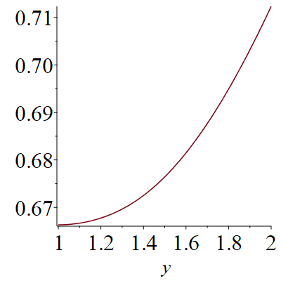
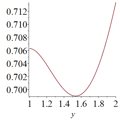
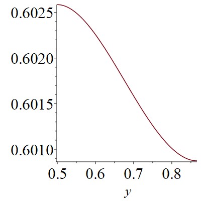
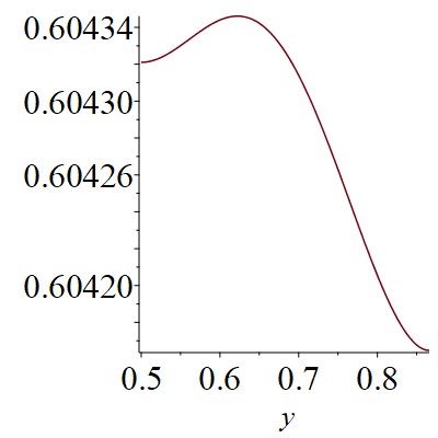
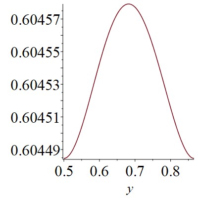
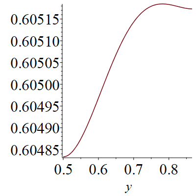
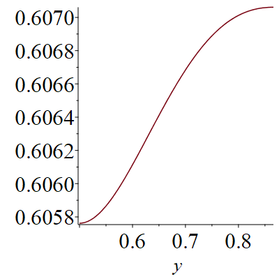
Figure 2.
The shape of ( θ ( α , z ) − π α M ( α , z ) ) 𝜃 𝛼 𝑧 𝜋 𝛼 𝑀 𝛼 𝑧 \Big{(}\theta(\alpha,z)-\pi\alpha M(\alpha,z)\Big{)} Γ a subscript Γ 𝑎 \Gamma_{a} α ≥ 1 𝛼 1 \alpha\geq 1
We shall prove that ( θ ( α , z ) − π α M ( α , z ) ) 𝜃 𝛼 𝑧 𝜋 𝛼 𝑀 𝛼 𝑧 \Big{(}\theta(\alpha,z)-\pi\alpha M(\alpha,z)\Big{)} Γ a subscript Γ 𝑎 \Gamma_{a} y = 1 𝑦 1 y=1 α 𝛼 \alpha α 𝛼 \alpha α 𝛼 \alpha
Note that z ∈ Γ a 𝑧 subscript Γ 𝑎 z\in\Gamma_{a} z = i y 𝑧 𝑖 𝑦 z=iy ( θ ( α , z ) − π α M ( α , z ) ) 𝜃 𝛼 𝑧 𝜋 𝛼 𝑀 𝛼 𝑧 \Big{(}\theta(\alpha,z)-\pi\alpha M(\alpha,z)\Big{)} Γ a subscript Γ 𝑎 \Gamma_{a}
( θ y ( α , i y ) − π α M y ( α , i y ) ) = θ y ( α , i y ) ⋅ ( 1 − π α M y ( α , i y ) θ y ( α , i y ) ) subscript 𝜃 𝑦 𝛼 𝑖 𝑦 𝜋 𝛼 subscript 𝑀 𝑦 𝛼 𝑖 𝑦 ⋅ subscript 𝜃 𝑦 𝛼 𝑖 𝑦 1 𝜋 𝛼 subscript 𝑀 𝑦 𝛼 𝑖 𝑦 subscript 𝜃 𝑦 𝛼 𝑖 𝑦 \displaystyle\Big{(}\theta_{y}(\alpha,iy)-\pi\alpha M_{y}(\alpha,iy)\Big{)}=\theta_{y}(\alpha,iy)\cdot\Big{(}1-\frac{\pi\alpha M_{y}(\alpha,iy)}{\theta_{y}(\alpha,iy)}\Big{)} (5.32)
One observes that(See Lemma 4.5
Lemma 5.2 .
Assume that α ≥ 1 𝛼 1 \alpha\geq 1 θ y ( α , i y ) ≥ 0 subscript 𝜃 𝑦 𝛼 𝑖 𝑦 0 \theta_{y}(\alpha,iy)\geq 0 y ≥ 1 𝑦 1 y\geq 1 " = " " " "=" y = 1 𝑦 1 y=1
To prove Theorem 5.2 ( θ ( α , z ) − π α M ( α , z ) ) 𝜃 𝛼 𝑧 𝜋 𝛼 𝑀 𝛼 𝑧 (\theta(\alpha,z)-\pi\alpha M(\alpha,z)) Γ a subscript Γ 𝑎 \Gamma_{a} α ≥ 101 100 𝛼 101 100 \alpha\geq\frac{101}{100}
Proposition 5.1 .
Assume that α ≥ 101 100 𝛼 101 100 \alpha\geq\frac{101}{100} ( θ ( α , z ) − π α M ( α , z ) ) 𝜃 𝛼 𝑧 𝜋 𝛼 𝑀 𝛼 𝑧 \Big{(}\theta(\alpha,z)-\pi\alpha M(\alpha,z)\Big{)} Γ a subscript Γ 𝑎 \Gamma_{a} y = 1 𝑦 1 y=1 α 𝛼 \alpha
•
( 1 ) 1 (1) if θ y y ( α , i ) ≥ π α M y y ( α , i ) subscript 𝜃 𝑦 𝑦 𝛼 𝑖 𝜋 𝛼 subscript 𝑀 𝑦 𝑦 𝛼 𝑖 \theta_{yy}(\alpha,i)\geq\pi\alpha M_{yy}(\alpha,i) , then ( θ ( α , z ) − π α M ( α , z ) ) 𝜃 𝛼 𝑧 𝜋 𝛼 𝑀 𝛼 𝑧 \Big{(}\theta(\alpha,z)-\pi\alpha M(\alpha,z)\Big{)} is increasing on Γ a subscript Γ 𝑎 \Gamma_{a} , and
min z ∈ Γ a ( θ ( α , z ) − π α M ( α , z ) ) is achieved at i . subscript 𝑧 subscript Γ 𝑎 𝜃 𝛼 𝑧 𝜋 𝛼 𝑀 𝛼 𝑧 is achieved at 𝑖 \min_{z\in\Gamma_{a}}\Big{(}\theta(\alpha,z)-\pi\alpha M(\alpha,z)\Big{)}\;\;\hbox{is achieved at}\;\;i.
•
( 2 ) 2 (2) if θ y y ( α , i ) < π α M y y ( α , i ) subscript 𝜃 𝑦 𝑦 𝛼 𝑖 𝜋 𝛼 subscript 𝑀 𝑦 𝑦 𝛼 𝑖 \theta_{yy}(\alpha,i)<\pi\alpha M_{yy}(\alpha,i) , then ( θ ( α , z ) − π α M ( α , z ) ) 𝜃 𝛼 𝑧 𝜋 𝛼 𝑀 𝛼 𝑧 \Big{(}\theta(\alpha,z)-\pi\alpha M(\alpha,z)\Big{)} is first decreasing then increasing on Γ a subscript Γ 𝑎 \Gamma_{a} , and
min z ∈ Γ a ( θ ( α , z ) − π α M ( α , z ) ) is achieved at i y α , where y α > 1 . subscript 𝑧 subscript Γ 𝑎 𝜃 𝛼 𝑧 𝜋 𝛼 𝑀 𝛼 𝑧 is achieved at 𝑖 subscript 𝑦 𝛼 where subscript 𝑦 𝛼
1 \min_{z\in\Gamma_{a}}\Big{(}\theta(\alpha,z)-\pi\alpha M(\alpha,z)\Big{)}\;\;\hbox{is achieved at}\;\;iy_{\alpha},\;\;\hbox{where}\;\;y_{\alpha}>1.
The shapes of ( θ ( α , z ) − π α M ( α , z ) ) 𝜃 𝛼 𝑧 𝜋 𝛼 𝑀 𝛼 𝑧 \Big{(}\theta(\alpha,z)-\pi\alpha M(\alpha,z)\Big{)} Γ a subscript Γ 𝑎 \Gamma_{a} α 𝛼 \alpha 2 5.1 θ y y ( α , i ) = π α M y y ( α , i ) subscript 𝜃 𝑦 𝑦 𝛼 𝑖 𝜋 𝛼 subscript 𝑀 𝑦 𝑦 𝛼 𝑖 \theta_{yy}(\alpha,i)=\pi\alpha M_{yy}(\alpha,i)
Lemma 5.3 .
Assume that α ≥ 101 100 𝛼 101 100 \alpha\geq\frac{101}{100}
•
( 1 ) : : 1 absent (1): θ y y ( α , i ) = π α M y y ( α , i ) subscript 𝜃 𝑦 𝑦 𝛼 𝑖 𝜋 𝛼 subscript 𝑀 𝑦 𝑦 𝛼 𝑖 \theta_{yy}(\alpha,i)=\pi\alpha M_{yy}(\alpha,i) admits only one solution, i.e., α = 1.117687748 ⋯ 𝛼 1.117687748 ⋯ \alpha=1.117687748\cdots ;
•
( 2 ) : : 2 absent (2): θ y y ( α , i ) ≥ π α M y y ( α , i ) subscript 𝜃 𝑦 𝑦 𝛼 𝑖 𝜋 𝛼 subscript 𝑀 𝑦 𝑦 𝛼 𝑖 \theta_{yy}(\alpha,i)\geq\pi\alpha M_{yy}(\alpha,i) ⇔ ⇔ \Leftrightarrow α ≤ 1.117687748 ⋯ 𝛼 1.117687748 ⋯ \alpha\leq 1.117687748\cdots ;
•
( 3 ) : : 3 absent (3): θ y y ( α , i ) < π α M y y ( α , i ) subscript 𝜃 𝑦 𝑦 𝛼 𝑖 𝜋 𝛼 subscript 𝑀 𝑦 𝑦 𝛼 𝑖 \theta_{yy}(\alpha,i)<\pi\alpha M_{yy}(\alpha,i) ⇔ ⇔ \Leftrightarrow α > 1.117687748 ⋯ 𝛼 1.117687748 ⋯ \alpha>1.117687748\cdots .
Theorem 5.2 5.1 5.3 5.1 5.3
To prove Proposition 5.1 5.32 5.2
Lemma 5.4 .
Assume that α ≥ 101 100 𝛼 101 100 \alpha\geq\frac{101}{100}
•
( 1 ) : : 1 absent (1): for y ≥ 2 α 𝑦 2 𝛼 y\geq 2\alpha , θ y ( α , i y ) − π α M y ( α , i y ) > 0 subscript 𝜃 𝑦 𝛼 𝑖 𝑦 𝜋 𝛼 subscript 𝑀 𝑦 𝛼 𝑖 𝑦 0 \theta_{y}(\alpha,iy)-\pi\alpha M_{y}(\alpha,iy)>0 ;
•
( 2 ) : : 2 absent (2): for y ∈ [ 1 , 2 α ] 𝑦 1 2 𝛼 y\in[1,2\alpha] , ∂ y M y ( α , i y ) θ y ( α , i y ) ≤ 0 subscript 𝑦 subscript 𝑀 𝑦 𝛼 𝑖 𝑦 subscript 𝜃 𝑦 𝛼 𝑖 𝑦 0 \partial_{y}\frac{M_{y}(\alpha,iy)}{\theta_{y}(\alpha,iy)}\leq 0 .
While to prove Lemma 5.2
Lemma 5.5 .
•
( 1 ) : : 1 absent (1): for α ≥ 9 8 𝛼 9 8 \alpha\geq\frac{9}{8} , θ y y ( α , i ) < π α M y y ( α , i ) subscript 𝜃 𝑦 𝑦 𝛼 𝑖 𝜋 𝛼 subscript 𝑀 𝑦 𝑦 𝛼 𝑖 \theta_{yy}(\alpha,i)<\pi\alpha M_{yy}(\alpha,i) ;
•
( 2 ) : : 2 absent (2): for α ∈ [ 1 , 9 8 ] 𝛼 1 9 8 \alpha\in[1,\frac{9}{8}] ,
∂ α ( α M y ( α , i ) θ y ( α , i ) ) > 0 subscript 𝛼 𝛼 subscript 𝑀 𝑦 𝛼 𝑖 subscript 𝜃 𝑦 𝛼 𝑖 0 \partial_{\alpha}\big{(}\frac{\alpha M_{y}(\alpha,i)}{\theta_{y}(\alpha,i)}\big{)}>0 .
Now by the reduction(Proposition 5.1 5.3 5.4 5.5 ( 1 ) 1 (1) 5.4 ( 2 ) 2 (2) 5.4 5.5
By Lemmas 3.2 3.3
Lemma 5.6 .
An exponentially decaying expansion for ( θ y ( α , i y ) − π α M y ( α , i y ) ) subscript 𝜃 𝑦 𝛼 𝑖 𝑦 𝜋 𝛼 subscript 𝑀 𝑦 𝛼 𝑖 𝑦 \Big{(}\theta_{y}(\alpha,iy)-\pi\alpha M_{y}(\alpha,iy)\Big{)}
θ y ( α , i y ) − π α M y ( α , i y ) = subscript 𝜃 𝑦 𝛼 𝑖 𝑦 𝜋 𝛼 subscript 𝑀 𝑦 𝛼 𝑖 𝑦 absent \displaystyle\theta_{y}(\alpha,iy)-\pi\alpha M_{y}(\alpha,iy)= 1 y α α 3 ∑ n ∈ ℤ ( α 2 ( π 2 n 4 α 2 y 2 − 2 π α y n 2 + 1 4 ) ϑ ( y α ; 0 ) \displaystyle\frac{1}{\sqrt{\frac{y}{\alpha}}\alpha^{3}}\sum_{n\in\mathbb{Z}}\Big{(}\alpha^{2}(\pi^{2}n^{4}\alpha^{2}y^{2}-2\pi\alpha yn^{2}+\frac{1}{4})\vartheta(\frac{y}{\alpha};0)
− α y ϑ X ( y α ; 0 ) − y 2 ϑ X X ( y α ; 0 ) ) ⋅ e − π α y n 2 . \displaystyle-\alpha y\vartheta_{X}(\frac{y}{\alpha};0)-y^{2}\vartheta_{XX}(\frac{y}{\alpha};0)\Big{)}\cdot e^{-\pi\alpha yn^{2}}.
Based on the expansion in Lemma 5.6
R n ( α , y ) := ( α 2 ( π 2 n 4 α 2 y 2 − 2 π α y n 2 + 1 4 ) ϑ ( y α ; 0 ) − α y ϑ X ( y α ; 0 ) − y 2 ϑ X X ( y α ; 0 ) ) . assign subscript 𝑅 𝑛 𝛼 𝑦 superscript 𝛼 2 superscript 𝜋 2 superscript 𝑛 4 superscript 𝛼 2 superscript 𝑦 2 2 𝜋 𝛼 𝑦 superscript 𝑛 2 1 4 italic-ϑ 𝑦 𝛼 0
𝛼 𝑦 subscript italic-ϑ 𝑋 𝑦 𝛼 0
superscript 𝑦 2 subscript italic-ϑ 𝑋 𝑋 𝑦 𝛼 0
\displaystyle R_{n}(\alpha,y):=\Big{(}\alpha^{2}(\pi^{2}n^{4}\alpha^{2}y^{2}-2\pi\alpha yn^{2}+\frac{1}{4})\vartheta(\frac{y}{\alpha};0)-\alpha y\vartheta_{X}(\frac{y}{\alpha};0)-y^{2}\vartheta_{XX}(\frac{y}{\alpha};0)\Big{)}. (5.33)
Then one has the summation
θ y ( α , i y ) − π α M y ( α , i y ) = subscript 𝜃 𝑦 𝛼 𝑖 𝑦 𝜋 𝛼 subscript 𝑀 𝑦 𝛼 𝑖 𝑦 absent \displaystyle\theta_{y}(\alpha,iy)-\pi\alpha M_{y}(\alpha,iy)= 1 y α α 3 ∑ n ∈ ℤ R n ( α , y ) ⋅ e − π α y n 2 1 𝑦 𝛼 superscript 𝛼 3 subscript 𝑛 ℤ ⋅ subscript 𝑅 𝑛 𝛼 𝑦 superscript 𝑒 𝜋 𝛼 𝑦 superscript 𝑛 2 \displaystyle\frac{1}{\sqrt{\frac{y}{\alpha}}\alpha^{3}}\sum_{n\in\mathbb{Z}}R_{n}(\alpha,y)\cdot e^{-\pi\alpha yn^{2}} (5.34)
Therefore, item ( 1 ) 1 (1) 5.4 5.34
Lemma 5.7 .
Assume that α ≥ 101 100 𝛼 101 100 \alpha\geq\frac{101}{100}
R n ( α , y ) > 0 for y α ≥ 2 , ∀ n ∈ ℤ . formulae-sequence subscript 𝑅 𝑛 𝛼 𝑦 0 for 𝑦 𝛼 2 for-all 𝑛 ℤ \displaystyle R_{n}(\alpha,y)>0\;\;\hbox{for}\;\;\frac{y}{\alpha}\geq 2,\;\;\forall n\in\mathbb{Z}.
In fact, from the explicit expressions of ϑ ( y α ; 0 ) , ϑ X ( y α ; 0 ) , ϑ X X ( y α ; 0 ) italic-ϑ 𝑦 𝛼 0
subscript italic-ϑ 𝑋 𝑦 𝛼 0
subscript italic-ϑ 𝑋 𝑋 𝑦 𝛼 0
\vartheta(\frac{y}{\alpha};0),\vartheta_{X}(\frac{y}{\alpha};0),\vartheta_{XX}(\frac{y}{\alpha};0) 2.5
ϑ ( y α ; 0 ) ≥ 1 , ϑ X ( y α ; 0 ) ≤ 0 , − ϑ X X ( y α ; 0 ) ≤ 4 π 2 e − π y α ( if y α ≥ 2 ) . formulae-sequence italic-ϑ 𝑦 𝛼 0
1 formulae-sequence subscript italic-ϑ 𝑋 𝑦 𝛼 0
0 subscript italic-ϑ 𝑋 𝑋 𝑦 𝛼 0
4 superscript 𝜋 2 superscript 𝑒 𝜋 𝑦 𝛼 if 𝑦 𝛼 2 \vartheta(\frac{y}{\alpha};0)\geq 1,\;\;\vartheta_{X}(\frac{y}{\alpha};0)\leq 0,\;\;-\vartheta_{XX}(\frac{y}{\alpha};0)\leq 4\pi^{2}e^{-\pi\frac{y}{\alpha}}(\hbox{if}\;\;\frac{y}{\alpha}\geq 2).
These estimates above will lead to Lemma 5.7 5.33
It remains to prove item ( 2 ) 2 (2) 5.4 5.5 ( θ y ( α , i y ) − π α M y ( α , i y ) ) subscript 𝜃 𝑦 𝛼 𝑖 𝑦 𝜋 𝛼 subscript 𝑀 𝑦 𝛼 𝑖 𝑦 \Big{(}\theta_{y}(\alpha,iy)-\pi\alpha M_{y}(\alpha,iy)\Big{)}
X a : : subscript 𝑋 𝑎 absent \displaystyle X_{a}: = X a ( α , y ) := ∑ n , m ( n 2 − m 2 y 2 ) e − π α ( y n 2 + m 2 y ) absent subscript 𝑋 𝑎 𝛼 𝑦 assign subscript 𝑛 𝑚
superscript 𝑛 2 superscript 𝑚 2 superscript 𝑦 2 superscript 𝑒 𝜋 𝛼 𝑦 superscript 𝑛 2 superscript 𝑚 2 𝑦 \displaystyle=X_{a}(\alpha,y):=\sum_{n,m}(n^{2}-\frac{m^{2}}{y^{2}})e^{-\pi\alpha(yn^{2}+\frac{m^{2}}{y})} (5.35)
X b : : subscript 𝑋 𝑏 absent \displaystyle X_{b}: = X b ( α , y ) := ∑ n , m ( y n 4 − m 4 y 3 ) e − π α ( y n 2 + m 2 y ) . absent subscript 𝑋 𝑏 𝛼 𝑦 assign subscript 𝑛 𝑚
𝑦 superscript 𝑛 4 superscript 𝑚 4 superscript 𝑦 3 superscript 𝑒 𝜋 𝛼 𝑦 superscript 𝑛 2 superscript 𝑚 2 𝑦 \displaystyle=X_{b}(\alpha,y):={\sum_{n,m}(yn^{4}-\frac{m^{4}}{y^{3}})e^{-\pi\alpha(yn^{2}+\frac{m^{2}}{y})}}.
Then
∂ y X a : : subscript 𝑦 subscript 𝑋 𝑎 absent \displaystyle\partial_{y}X_{a}: = ∂ y X a ( α , y ) := − ∑ n , m ( π α ( n 2 − m 2 y 2 ) 2 − 2 m 2 y 3 ) e − π α ( y n 2 + m 2 y ) absent subscript 𝑦 subscript 𝑋 𝑎 𝛼 𝑦 assign subscript 𝑛 𝑚
𝜋 𝛼 superscript superscript 𝑛 2 superscript 𝑚 2 superscript 𝑦 2 2 2 superscript 𝑚 2 superscript 𝑦 3 superscript 𝑒 𝜋 𝛼 𝑦 superscript 𝑛 2 superscript 𝑚 2 𝑦 \displaystyle=\partial_{y}X_{a}(\alpha,y):=-\sum_{n,m}(\pi\alpha(n^{2}-\frac{m^{2}}{y^{2}})^{2}-\frac{2m^{2}}{y^{3}})e^{-\pi\alpha(yn^{2}+\frac{m^{2}}{y})} (5.36)
∂ y X b : : subscript 𝑦 subscript 𝑋 𝑏 absent \displaystyle\partial_{y}X_{b}: = ∂ y X b ( α , y ) := − ∑ n , m ( π α y ( n 4 − m 4 y 4 ) ( n 2 − m 2 y 2 ) − ( n 4 + 3 m 4 y 4 ) ) e − π α ( y n 2 + m 2 y ) . absent subscript 𝑦 subscript 𝑋 𝑏 𝛼 𝑦 assign subscript 𝑛 𝑚
𝜋 𝛼 𝑦 superscript 𝑛 4 superscript 𝑚 4 superscript 𝑦 4 superscript 𝑛 2 superscript 𝑚 2 superscript 𝑦 2 superscript 𝑛 4 3 superscript 𝑚 4 superscript 𝑦 4 superscript 𝑒 𝜋 𝛼 𝑦 superscript 𝑛 2 superscript 𝑚 2 𝑦 \displaystyle=\partial_{y}X_{b}(\alpha,y):=-{\sum_{n,m}(\pi\alpha y(n^{4}-\frac{m^{4}}{y^{4}})(n^{2}-\frac{m^{2}}{y^{2}})-(n^{4}+\frac{3m^{4}}{y^{4}}))e^{-\pi\alpha(yn^{2}+\frac{m^{2}}{y})}}.
Therefore, one has the following simplifications immediately(Lemmas 5.8 5.9
Lemma 5.8 .
A relation between θ ( α , i y ) , M ( α , i y ) 𝜃 𝛼 𝑖 𝑦 𝑀 𝛼 𝑖 𝑦
\theta(\alpha,iy),M(\alpha,iy) X a , X b subscript 𝑋 𝑎 subscript 𝑋 𝑏
X_{a},X_{b}
θ y ( α , i y ) subscript 𝜃 𝑦 𝛼 𝑖 𝑦 \displaystyle\theta_{y}(\alpha,iy) = − π α X a , π α M y ( α , i y ) = π α X a − ( π α ) 2 X b ; formulae-sequence absent 𝜋 𝛼 subscript 𝑋 𝑎 𝜋 𝛼 subscript 𝑀 𝑦 𝛼 𝑖 𝑦 𝜋 𝛼 subscript 𝑋 𝑎 superscript 𝜋 𝛼 2 subscript 𝑋 𝑏 \displaystyle=-\pi\alpha X_{a},\;\;\pi\alpha M_{y}(\alpha,iy)=\pi\alpha X_{a}-(\pi\alpha)^{2}X_{b};
θ y y ( α , i y ) subscript 𝜃 𝑦 𝑦 𝛼 𝑖 𝑦 \displaystyle\theta_{yy}(\alpha,iy) = − π α ∂ y X a , π α M y y ( α , i y ) = π α ∂ y X a − ( π α ) 2 ∂ y X b . formulae-sequence absent 𝜋 𝛼 subscript 𝑦 subscript 𝑋 𝑎 𝜋 𝛼 subscript 𝑀 𝑦 𝑦 𝛼 𝑖 𝑦 𝜋 𝛼 subscript 𝑦 subscript 𝑋 𝑎 superscript 𝜋 𝛼 2 subscript 𝑦 subscript 𝑋 𝑏 \displaystyle=-\pi\alpha\partial_{y}X_{a},\;\;\pi\alpha M_{yy}(\alpha,iy)=\pi\alpha\partial_{y}X_{a}-(\pi\alpha)^{2}\partial_{y}X_{b}.
Lemma 5.9 .
A relation between M y ( α , i y ) θ y ( α , i y ) subscript 𝑀 𝑦 𝛼 𝑖 𝑦 subscript 𝜃 𝑦 𝛼 𝑖 𝑦 \frac{M_{y}(\alpha,iy)}{\theta_{y}(\alpha,iy)} X b X a subscript 𝑋 𝑏 subscript 𝑋 𝑎 \frac{X_{b}}{X_{a}}
M y ( α , i y ) θ y ( α , i y ) = − 1 π α + X b X a , M y y ( α , i y ) θ y y ( α , i y ) = − 1 π α + ∂ y X b ∂ y X a . formulae-sequence subscript 𝑀 𝑦 𝛼 𝑖 𝑦 subscript 𝜃 𝑦 𝛼 𝑖 𝑦 1 𝜋 𝛼 subscript 𝑋 𝑏 subscript 𝑋 𝑎 subscript 𝑀 𝑦 𝑦 𝛼 𝑖 𝑦 subscript 𝜃 𝑦 𝑦 𝛼 𝑖 𝑦 1 𝜋 𝛼 subscript 𝑦 subscript 𝑋 𝑏 subscript 𝑦 subscript 𝑋 𝑎 \displaystyle\frac{M_{y}(\alpha,iy)}{\theta_{y}(\alpha,iy)}=-\frac{1}{\pi\alpha}+\frac{X_{b}}{X_{a}},\;\;\frac{M_{yy}(\alpha,iy)}{\theta_{yy}(\alpha,iy)}=-\frac{1}{\pi\alpha}+\frac{\partial_{y}X_{b}}{\partial_{y}X_{a}}.
With these simplifications(Lemmas 5.8 5.9 ( 2 ) 2 (2) 5.4 5.5 5.12
Lemma 5.10 (=item ( 2 ) 2 (2) 5.4 .
Assume that α ≥ 101 100 𝛼 101 100 \alpha\geq\frac{101}{100} ∂ y X b X a ≤ 0 for y ∈ [ 1 , 2 α ] . subscript 𝑦 subscript 𝑋 𝑏 subscript 𝑋 𝑎 0 for 𝑦 1 2 𝛼 \partial_{y}\frac{X_{b}}{X_{a}}\leq 0\;\;\hbox{for}\;\;y\in[1,2\alpha].
Lemma 5.11 (=Lemma 5.5 .
•
( 1 ) : : 1 absent (1): for α ≥ 9 8 𝛼 9 8 \alpha\geq\frac{9}{8} , 2 π α ∂ y X a ∣ y = 1 ∂ y X b ∣ y = 1 < 1 2 𝜋 𝛼 evaluated-at subscript 𝑦 subscript 𝑋 𝑎 𝑦 1 evaluated-at subscript 𝑦 subscript 𝑋 𝑏 𝑦 1 1 \frac{2}{\pi\alpha}\frac{\partial_{y}X_{a}\mid_{y=1}}{\partial_{y}X_{b}\mid_{y=1}}<1 ;
•
( 2 ) : : 2 absent (2): for α ∈ [ 1 , 9 8 ] 𝛼 1 9 8 \alpha\in[1,\frac{9}{8}] ,
1 α ∂ y X a ∣ y = 1 ∂ y X b ∣ y = 1 < 0 1 𝛼 evaluated-at subscript 𝑦 subscript 𝑋 𝑎 𝑦 1 evaluated-at subscript 𝑦 subscript 𝑋 𝑏 𝑦 1 0 \frac{1}{\alpha}\frac{\partial_{y}X_{a}\mid_{y=1}}{\partial_{y}X_{b}\mid_{y=1}}<0 .
Lemma 5.12 .
Assume that α ≥ 1 𝛼 1 \alpha\geq 1 ∂ y X b ∣ y = 1 < 0 . evaluated-at subscript 𝑦 subscript 𝑋 𝑏 𝑦 1 0 \partial_{y}X_{b}\mid_{y=1}<0.
To prove Lemma 5.10 X b ∣ y = 1 = X a ∣ y = 1 = 0 evaluated-at subscript 𝑋 𝑏 𝑦 1 evaluated-at subscript 𝑋 𝑎 𝑦 1 0 X_{b}\mid_{y=1}=X_{a}\mid_{y=1}=0 y = 1 𝑦 1 y=1 y = 1 𝑦 1 y=1
Lemma 5.13 .
Assume that α ≥ 101 100 𝛼 101 100 \alpha\geq\frac{101}{100}
•
( 1 ) : : 1 absent (1): for y ∈ [ 1 , 11 10 α ] 𝑦 1 11 10 𝛼 y\in[1,\frac{11}{10}\alpha] , ∂ y ∂ y X b ∂ y X a < 0 subscript 𝑦 subscript 𝑦 subscript 𝑋 𝑏 subscript 𝑦 subscript 𝑋 𝑎 0 \partial_{y}\frac{\partial_{y}X_{b}}{\partial_{y}X_{a}}<0 ;
•
( 2 ) : : 2 absent (2): for y ∈ [ 11 10 α , 2 α ] 𝑦 11 10 𝛼 2 𝛼 y\in[\frac{11}{10}\alpha,2\alpha] ,
∂ y X b X a < 0 subscript 𝑦 subscript 𝑋 𝑏 subscript 𝑋 𝑎 0 \partial_{y}\frac{X_{b}}{X_{a}}<0 .
Note that (since X b ∣ y = 1 = X a ∣ y = 1 = 0 evaluated-at subscript 𝑋 𝑏 𝑦 1 evaluated-at subscript 𝑋 𝑎 𝑦 1 0 X_{b}\mid_{y=1}=X_{a}\mid_{y=1}=0 [1 ] ), item ( 1 ) 1 (1) 5.13 ∂ y X b X a < 0 subscript 𝑦 subscript 𝑋 𝑏 subscript 𝑋 𝑎 0 \partial_{y}\frac{X_{b}}{X_{a}}<0 y ∈ [ 1 , 11 10 α ] 𝑦 1 11 10 𝛼 y\in[1,\frac{11}{10}\alpha] 5.13 5.10 5.12 5.13
Recall the expressions in (5.35
𝒜 a : : subscript 𝒜 𝑎 absent \displaystyle\mathcal{A}_{a}: = 𝒜 a ( α , y ) := ∑ n 2 + m 2 ≤ 2 ( n 2 − m 2 y 2 ) e − π α ( y n 2 + m 2 y ) , absent subscript 𝒜 𝑎 𝛼 𝑦 assign subscript superscript 𝑛 2 superscript 𝑚 2 2 superscript 𝑛 2 superscript 𝑚 2 superscript 𝑦 2 superscript 𝑒 𝜋 𝛼 𝑦 superscript 𝑛 2 superscript 𝑚 2 𝑦 \displaystyle=\mathcal{A}_{a}(\alpha,y):=\sum_{n^{2}+m^{2}\leq 2}(n^{2}-\frac{m^{2}}{y^{2}})e^{-\pi\alpha(yn^{2}+\frac{m^{2}}{y})}, (5.37)
𝒜 e : : subscript 𝒜 𝑒 absent \displaystyle\mathcal{A}_{e}: = 𝒜 e ( α , y ) := ∑ n 2 + m 2 ≥ 3 ( n 2 − m 2 y 2 ) e − π α ( y n 2 + m 2 y ) absent subscript 𝒜 𝑒 𝛼 𝑦 assign subscript superscript 𝑛 2 superscript 𝑚 2 3 superscript 𝑛 2 superscript 𝑚 2 superscript 𝑦 2 superscript 𝑒 𝜋 𝛼 𝑦 superscript 𝑛 2 superscript 𝑚 2 𝑦 \displaystyle=\mathcal{A}_{e}(\alpha,y):=\sum_{n^{2}+m^{2}\geq 3}(n^{2}-\frac{m^{2}}{y^{2}})e^{-\pi\alpha(yn^{2}+\frac{m^{2}}{y})}
being the dominated and error terms of X a subscript 𝑋 𝑎 X_{a} X a = 𝒜 a + 𝒜 e . subscript 𝑋 𝑎 subscript 𝒜 𝑎 subscript 𝒜 𝑒 X_{a}=\mathcal{A}_{a}+\mathcal{A}_{e}. X b subscript 𝑋 𝑏 X_{b}
ℬ a : : subscript ℬ 𝑎 absent \displaystyle\mathcal{B}_{a}: = ℬ a ( α , y ) := ∑ n 2 + m 2 ≤ 2 ( y n 4 − m 4 y 3 ) e − π α ( y n 2 + m 2 y ) absent subscript ℬ 𝑎 𝛼 𝑦 assign subscript superscript 𝑛 2 superscript 𝑚 2 2 𝑦 superscript 𝑛 4 superscript 𝑚 4 superscript 𝑦 3 superscript 𝑒 𝜋 𝛼 𝑦 superscript 𝑛 2 superscript 𝑚 2 𝑦 \displaystyle=\mathcal{B}_{a}(\alpha,y):={\sum_{n^{2}+m^{2}\leq 2}(yn^{4}-\frac{m^{4}}{y^{3}})e^{-\pi\alpha(yn^{2}+\frac{m^{2}}{y})}} (5.38)
ℬ e : : subscript ℬ 𝑒 absent \displaystyle\mathcal{B}_{e}: = ℬ a ( α , y ) := ∑ n 2 + m 2 ≥ 3 ( y n 4 − m 4 y 3 ) e − π α ( y n 2 + m 2 y ) . absent subscript ℬ 𝑎 𝛼 𝑦 assign subscript superscript 𝑛 2 superscript 𝑚 2 3 𝑦 superscript 𝑛 4 superscript 𝑚 4 superscript 𝑦 3 superscript 𝑒 𝜋 𝛼 𝑦 superscript 𝑛 2 superscript 𝑚 2 𝑦 \displaystyle=\mathcal{B}_{a}(\alpha,y):={\sum_{n^{2}+m^{2}\geq 3}(yn^{4}-\frac{m^{4}}{y^{3}})e^{-\pi\alpha(yn^{2}+\frac{m^{2}}{y})}}.
being the the dominated and error terms of X b subscript 𝑋 𝑏 X_{b} X b = ℬ a + ℬ e . subscript 𝑋 𝑏 subscript ℬ 𝑎 subscript ℬ 𝑒 X_{b}=\mathcal{B}_{a}+\mathcal{B}_{e}.
Explicitly, one has
𝒜 a subscript 𝒜 𝑎 \displaystyle\mathcal{A}_{a} = 2 e − π α y − 2 y 2 e − π α y + 4 ( 1 − 1 y 2 ) e − π α ( y + 1 y ) , absent 2 superscript 𝑒 𝜋 𝛼 𝑦 2 superscript 𝑦 2 superscript 𝑒 𝜋 𝛼 𝑦 4 1 1 superscript 𝑦 2 superscript 𝑒 𝜋 𝛼 𝑦 1 𝑦 \displaystyle=2e^{-\pi\alpha y}-\frac{2}{y^{2}}e^{-\frac{\pi\alpha}{y}}+4(1-\frac{1}{y^{2}})e^{-\pi\alpha(y+\frac{1}{y})}, (5.39)
ℬ a subscript ℬ 𝑎 \displaystyle\mathcal{B}_{a} = 2 y e − π α y − 2 y 3 e − π α y + 4 ( y − 1 y 3 ) e − π α ( y + 1 y ) . absent 2 𝑦 superscript 𝑒 𝜋 𝛼 𝑦 2 superscript 𝑦 3 superscript 𝑒 𝜋 𝛼 𝑦 4 𝑦 1 superscript 𝑦 3 superscript 𝑒 𝜋 𝛼 𝑦 1 𝑦 \displaystyle=2ye^{-\pi\alpha y}-\frac{2}{y^{3}}e^{-\frac{\pi\alpha}{y}}+4(y-\frac{1}{y^{3}})e^{-\pi\alpha(y+\frac{1}{y})}.
𝒜 e , ℬ e subscript 𝒜 𝑒 subscript ℬ 𝑒
\mathcal{A}_{e},\mathcal{B}_{e} X a , X b subscript 𝑋 𝑎 subscript 𝑋 𝑏
X_{a},X_{b}
∣ 𝒜 e 𝒜 a ∣ delimited-∣∣ subscript 𝒜 𝑒 subscript 𝒜 𝑎 \displaystyle\mid\frac{\mathcal{A}_{e}}{\mathcal{A}_{a}}\mid = O ( e − 3 π α y ) , ∣ ℬ e ℬ a ∣ = O ( e − 3 π α y ) for y ∈ [ 11 10 , 2 α ] , α ≥ 1 , formulae-sequence formulae-sequence absent 𝑂 superscript 𝑒 3 𝜋 𝛼 𝑦 delimited-∣∣ subscript ℬ 𝑒 subscript ℬ 𝑎 𝑂 superscript 𝑒 3 𝜋 𝛼 𝑦 for 𝑦 11 10 2 𝛼 𝛼 1 \displaystyle=O(e^{-\frac{3\pi\alpha}{y}}),\;\;\mid\frac{\mathcal{B}_{e}}{\mathcal{B}_{a}}\mid=O(e^{-\frac{3\pi\alpha}{y}})\;\;\hbox{for}\;\;y\in[\frac{11}{10},2\alpha],\;\alpha\geq 1, (5.40)
∣ ∂ y 𝒜 e ∂ y 𝒜 a ∣ delimited-∣∣ subscript 𝑦 subscript 𝒜 𝑒 subscript 𝑦 subscript 𝒜 𝑎 \displaystyle\mid\frac{\partial_{y}\mathcal{A}_{e}}{\partial_{y}\mathcal{A}_{a}}\mid = O ( e − 3 π α y ) , ∣ ∂ y ℬ e ∂ y ℬ a ∣ = O ( e − 3 π α y ) for y ∈ [ 1 , 11 10 α ] , α ≥ 1 . formulae-sequence formulae-sequence absent 𝑂 superscript 𝑒 3 𝜋 𝛼 𝑦 delimited-∣∣ subscript 𝑦 subscript ℬ 𝑒 subscript 𝑦 subscript ℬ 𝑎 𝑂 superscript 𝑒 3 𝜋 𝛼 𝑦 for 𝑦 1 11 10 𝛼 𝛼 1 \displaystyle=O(e^{-\frac{3\pi\alpha}{y}}),\;\;\mid\frac{\partial_{y}\mathcal{B}_{e}}{\partial_{y}\mathcal{B}_{a}}\mid=O(e^{-\frac{3\pi\alpha}{y}})\;\;\hbox{for}\;\;y\in[1,\frac{11}{10}\alpha],\;\alpha\geq 1.
At this stage, we shall state a monotonicity property on ℬ a 𝒜 a subscript ℬ 𝑎 subscript 𝒜 𝑎 \frac{\mathcal{B}_{a}}{\mathcal{A}_{a}} ∂ y ℬ a ∂ y 𝒜 a subscript 𝑦 subscript ℬ 𝑎 subscript 𝑦 subscript 𝒜 𝑎 \frac{\partial_{y}\mathcal{B}_{a}}{\partial_{y}\mathcal{A}_{a}} 5.39
Lemma 5.14 .
Assume that α ≥ 101 100 𝛼 101 100 \alpha\geq\frac{101}{100}
•
( 1 ) : : 1 absent (1): for y ∈ [ 1 , 11 10 α ] 𝑦 1 11 10 𝛼 y\in[1,\frac{11}{10}\alpha] , ∂ y ∂ y ℬ a ∂ y 𝒜 a < 0 subscript 𝑦 subscript 𝑦 subscript ℬ 𝑎 subscript 𝑦 subscript 𝒜 𝑎 0 \partial_{y}\frac{\partial_{y}\mathcal{B}_{a}}{\partial_{y}\mathcal{A}_{a}}<0 or equivalently,
∂ y y ℬ a ⋅ ∂ y 𝒜 a − ∂ y ℬ a ⋅ ∂ y y 𝒜 a < 0 subscript 𝑦 𝑦 ⋅ subscript ℬ 𝑎 subscript 𝑦 subscript 𝒜 𝑎 subscript 𝑦 ⋅ subscript ℬ 𝑎 subscript 𝑦 𝑦 subscript 𝒜 𝑎 0 \partial_{yy}\mathcal{B}_{a}\cdot\partial_{y}\mathcal{A}_{a}-\partial_{y}\mathcal{B}_{a}\cdot\partial_{yy}\mathcal{A}_{a}<0 ;
•
( 2 ) : : 2 absent (2): for y ∈ [ 11 10 α , 2 α ] 𝑦 11 10 𝛼 2 𝛼 y\in[\frac{11}{10}\alpha,2\alpha] , ∂ y ℬ a 𝒜 a subscript 𝑦 subscript ℬ 𝑎 subscript 𝒜 𝑎 \partial_{y}\frac{\mathcal{B}_{a}}{\mathcal{A}_{a}}
or equivalently,
∂ y ℬ a ⋅ 𝒜 a − ℬ a ⋅ ∂ y 𝒜 a < 0 subscript 𝑦 ⋅ subscript ℬ 𝑎 subscript 𝒜 𝑎 ⋅ subscript ℬ 𝑎 subscript 𝑦 subscript 𝒜 𝑎 0 \partial_{y}\mathcal{B}_{a}\cdot\mathcal{A}_{a}-\mathcal{B}_{a}\cdot\partial_{y}\mathcal{A}_{a}<0 .
Lemma 5.14 5.10 ( 2 ) 2 (2) 5.13
∂ y X b X a = 1 X a 2 ( ∂ y X b ⋅ X a − ∂ y X a ⋅ X b ) = 1 X a 2 ( ∂ y ℬ a ⋅ 𝒜 a − ∂ y 𝒜 a ⋅ ℬ a + ϵ I ) , subscript 𝑦 subscript 𝑋 𝑏 subscript 𝑋 𝑎 1 superscript subscript 𝑋 𝑎 2 subscript 𝑦 ⋅ subscript 𝑋 𝑏 subscript 𝑋 𝑎 subscript 𝑦 ⋅ subscript 𝑋 𝑎 subscript 𝑋 𝑏 1 superscript subscript 𝑋 𝑎 2 subscript 𝑦 ⋅ subscript ℬ 𝑎 subscript 𝒜 𝑎 subscript 𝑦 ⋅ subscript 𝒜 𝑎 subscript ℬ 𝑎 subscript italic-ϵ 𝐼 \displaystyle\partial_{y}\frac{X_{b}}{X_{a}}=\frac{1}{X_{a}^{2}}\Big{(}\partial_{y}X_{b}\cdot X_{a}-\partial_{y}X_{a}\cdot X_{b}\Big{)}=\frac{1}{X_{a}^{2}}\Big{(}\partial_{y}\mathcal{B}_{a}\cdot\mathcal{A}_{a}-\partial_{y}\mathcal{A}_{a}\cdot\mathcal{B}_{a}+\epsilon_{I}\Big{)}, (5.41)
where explicitly, the error term ϵ I subscript italic-ϵ 𝐼 \epsilon_{I}
ϵ I = ( ∂ y ℬ a 𝒜 e + ∂ y ℬ e 𝒜 a + ∂ y ℬ e 𝒜 e ) − ( ℬ a ∂ y 𝒜 e + ℬ e ∂ y 𝒜 a + ℬ e ∂ y 𝒜 e ) . subscript italic-ϵ 𝐼 subscript 𝑦 subscript ℬ 𝑎 subscript 𝒜 𝑒 subscript 𝑦 subscript ℬ 𝑒 subscript 𝒜 𝑎 subscript 𝑦 subscript ℬ 𝑒 subscript 𝒜 𝑒 subscript ℬ 𝑎 subscript 𝑦 subscript 𝒜 𝑒 subscript ℬ 𝑒 subscript 𝑦 subscript 𝒜 𝑎 subscript ℬ 𝑒 subscript 𝑦 subscript 𝒜 𝑒 \displaystyle\epsilon_{I}=(\partial_{y}\mathcal{B}_{a}\mathcal{A}_{e}+\partial_{y}\mathcal{B}_{e}\mathcal{A}_{a}+\partial_{y}\mathcal{B}_{e}\mathcal{A}_{e})-(\mathcal{B}_{a}\partial_{y}\mathcal{A}_{e}+\mathcal{B}_{e}\partial_{y}\mathcal{A}_{a}+\mathcal{B}_{e}\partial_{y}\mathcal{A}_{e}).
Comparing to the major term ( ∂ y ℬ a ⋅ 𝒜 a − ∂ y 𝒜 a ⋅ ℬ a ) subscript 𝑦 ⋅ subscript ℬ 𝑎 subscript 𝒜 𝑎 subscript 𝑦 ⋅ subscript 𝒜 𝑎 subscript ℬ 𝑎 \Big{(}\partial_{y}\mathcal{B}_{a}\cdot\mathcal{A}_{a}-\partial_{y}\mathcal{A}_{a}\cdot\mathcal{B}_{a}\Big{)} ϵ I subscript italic-ϵ 𝐼 \epsilon_{I} 𝒜 e , ℬ e , ∂ y 𝒜 e , ∂ y ℬ e subscript 𝒜 𝑒 subscript ℬ 𝑒 subscript 𝑦 subscript 𝒜 𝑒 subscript 𝑦 subscript ℬ 𝑒
\mathcal{A}_{e},\mathcal{B}_{e},\partial_{y}\mathcal{A}_{e},\partial_{y}\mathcal{B}_{e} 5.40
| ϵ I ∂ y ℬ a ⋅ 𝒜 a − ∂ y 𝒜 a ⋅ ℬ a | ≤ 1 2 for y ∈ [ 11 10 α , 2 α ] , α ≥ 101 100 . formulae-sequence subscript italic-ϵ 𝐼 subscript 𝑦 ⋅ subscript ℬ 𝑎 subscript 𝒜 𝑎 subscript 𝑦 ⋅ subscript 𝒜 𝑎 subscript ℬ 𝑎 1 2 for 𝑦 11 10 𝛼 2 𝛼 𝛼 101 100 \displaystyle|\frac{\epsilon_{I}}{\partial_{y}\mathcal{B}_{a}\cdot\mathcal{A}_{a}-\partial_{y}\mathcal{A}_{a}\cdot\mathcal{B}_{a}}|\leq\frac{1}{2}\;\;\hbox{for}\;\;y\in[\frac{11}{10}\alpha,2\alpha],\;\alpha\geq\frac{101}{100}. (5.42)
The upper bound 1 2 1 2 \frac{1}{2} 5.42 5.41 5.42 ( 2 ) 2 (2) 5.14 ( 2 ) 2 (2) 5.13
Similar steps and estimates work for ∂ y ∂ y X b ∂ y X a subscript 𝑦 subscript 𝑦 subscript 𝑋 𝑏 subscript 𝑦 subscript 𝑋 𝑎 \partial_{y}\frac{\partial_{y}X_{b}}{\partial_{y}X_{a}}
∂ y ∂ y X b ∂ y X a = 1 ∂ y X a 2 ( ∂ y y X b ⋅ ∂ y X a − ∂ y y X a ⋅ ∂ y X b ) = 1 ∂ y X a 2 ( ∂ y y ℬ a ⋅ ∂ y 𝒜 a − ∂ y y 𝒜 a ⋅ ∂ y ℬ a + ϵ I I ) , subscript 𝑦 subscript 𝑦 subscript 𝑋 𝑏 subscript 𝑦 subscript 𝑋 𝑎 1 subscript 𝑦 superscript subscript 𝑋 𝑎 2 subscript 𝑦 𝑦 ⋅ subscript 𝑋 𝑏 subscript 𝑦 subscript 𝑋 𝑎 subscript 𝑦 𝑦 ⋅ subscript 𝑋 𝑎 subscript 𝑦 subscript 𝑋 𝑏 1 subscript 𝑦 superscript subscript 𝑋 𝑎 2 subscript 𝑦 𝑦 ⋅ subscript ℬ 𝑎 subscript 𝑦 subscript 𝒜 𝑎 subscript 𝑦 𝑦 ⋅ subscript 𝒜 𝑎 subscript 𝑦 subscript ℬ 𝑎 subscript italic-ϵ 𝐼 𝐼 \displaystyle\partial_{y}\frac{\partial_{y}X_{b}}{\partial_{y}X_{a}}=\frac{1}{\partial_{y}X_{a}^{2}}\Big{(}\partial_{yy}X_{b}\cdot\partial_{y}X_{a}-\partial_{yy}X_{a}\cdot\partial_{y}X_{b}\Big{)}=\frac{1}{\partial_{y}X_{a}^{2}}\Big{(}\partial_{yy}\mathcal{B}_{a}\cdot\partial_{y}\mathcal{A}_{a}-\partial_{yy}\mathcal{A}_{a}\cdot\partial_{y}\mathcal{B}_{a}+\epsilon_{II}\Big{)}, (5.43)
where explicitly,
ϵ I I = ( ∂ y y ℬ a ∂ y 𝒜 e + ∂ y y ℬ e ∂ y 𝒜 a + ∂ y y ℬ e ∂ y 𝒜 e ) − ( ∂ y ℬ a ∂ y y 𝒜 e + ∂ y ℬ e ∂ y y 𝒜 a + ∂ y ℬ e ∂ y y 𝒜 e ) . subscript italic-ϵ 𝐼 𝐼 subscript 𝑦 𝑦 subscript ℬ 𝑎 subscript 𝑦 subscript 𝒜 𝑒 subscript 𝑦 𝑦 subscript ℬ 𝑒 subscript 𝑦 subscript 𝒜 𝑎 subscript 𝑦 𝑦 subscript ℬ 𝑒 subscript 𝑦 subscript 𝒜 𝑒 subscript 𝑦 subscript ℬ 𝑎 subscript 𝑦 𝑦 subscript 𝒜 𝑒 subscript 𝑦 subscript ℬ 𝑒 subscript 𝑦 𝑦 subscript 𝒜 𝑎 subscript 𝑦 subscript ℬ 𝑒 subscript 𝑦 𝑦 subscript 𝒜 𝑒 \displaystyle\epsilon_{II}=(\partial_{yy}\mathcal{B}_{a}\partial_{y}\mathcal{A}_{e}+\partial_{yy}\mathcal{B}_{e}\partial_{y}\mathcal{A}_{a}+\partial_{yy}\mathcal{B}_{e}\partial_{y}\mathcal{A}_{e})-(\partial_{y}\mathcal{B}_{a}\partial_{yy}\mathcal{A}_{e}+\partial_{y}\mathcal{B}_{e}\partial_{yy}\mathcal{A}_{a}+\partial_{y}\mathcal{B}_{e}\partial_{yy}\mathcal{A}_{e}).
And the remainder estimate holds
| ϵ I I ∂ y y X b ⋅ ∂ y X a − ∂ y y X a ⋅ ∂ y X b | ≤ 1 2 for y ∈ [ 1 , 11 10 α ] , α ≥ 101 100 . formulae-sequence subscript italic-ϵ 𝐼 𝐼 subscript 𝑦 𝑦 ⋅ subscript 𝑋 𝑏 subscript 𝑦 subscript 𝑋 𝑎 subscript 𝑦 𝑦 ⋅ subscript 𝑋 𝑎 subscript 𝑦 subscript 𝑋 𝑏 1 2 for 𝑦 1 11 10 𝛼 𝛼 101 100 \displaystyle|\frac{\epsilon_{II}}{\partial_{yy}X_{b}\cdot\partial_{y}X_{a}-\partial_{yy}X_{a}\cdot\partial_{y}X_{b}}|\leq\frac{1}{2}\;\;\hbox{for}\;\;y\in[1,\frac{11}{10}\alpha],\;\alpha\geq\frac{101}{100}. (5.44)
Therefore, (5.43 5.44 ( 1 ) 1 (1) 5.14 ( 1 ) 1 (1) 5.13
At the end of this Section, we give the proof of Lemmas 5.11 5.12 y = 1 𝑦 1 y=1 5.36
∂ y X a ∣ y = 1 evaluated-at subscript 𝑦 subscript 𝑋 𝑎 𝑦 1 \displaystyle\partial_{y}X_{a}\mid_{y=1} = − ∑ n , m ( π α ( n 2 − m 2 ) 2 − 2 m 2 ) e − π α ( n 2 + m 2 ) absent subscript 𝑛 𝑚
𝜋 𝛼 superscript superscript 𝑛 2 superscript 𝑚 2 2 2 superscript 𝑚 2 superscript 𝑒 𝜋 𝛼 superscript 𝑛 2 superscript 𝑚 2 \displaystyle=-\sum_{n,m}(\pi\alpha(n^{2}-m^{2})^{2}-2m^{2})e^{-\pi\alpha(n^{2}+m^{2})}
∂ y X b ∣ y = 1 evaluated-at subscript 𝑦 subscript 𝑋 𝑏 𝑦 1 \displaystyle\partial_{y}X_{b}\mid_{y=1} = − ∑ n , m ( π α ( n 4 − m 4 ) ( n 2 − m 2 ) − ( n 4 + 3 m 4 ) ) e − π α ( n 2 + m 2 ) . absent subscript 𝑛 𝑚
𝜋 𝛼 superscript 𝑛 4 superscript 𝑚 4 superscript 𝑛 2 superscript 𝑚 2 superscript 𝑛 4 3 superscript 𝑚 4 superscript 𝑒 𝜋 𝛼 superscript 𝑛 2 superscript 𝑚 2 \displaystyle=-\sum_{n,m}(\pi\alpha(n^{4}-m^{4})(n^{2}-m^{2})-(n^{4}+3m^{4}))e^{-\pi\alpha(n^{2}+m^{2})}.
Before going to the proof, we do some preparing work. As the same decomposition in (5.38
A : : 𝐴 absent \displaystyle A: = A ( α ) = ∑ n 2 + m 2 ≤ 2 ( π α ( n 2 − m 2 ) 2 − 2 m 2 ) e − π α ( n 2 + m 2 ) , absent 𝐴 𝛼 subscript superscript 𝑛 2 superscript 𝑚 2 2 𝜋 𝛼 superscript superscript 𝑛 2 superscript 𝑚 2 2 2 superscript 𝑚 2 superscript 𝑒 𝜋 𝛼 superscript 𝑛 2 superscript 𝑚 2 \displaystyle=A(\alpha)=\sum_{n^{2}+m^{2}\leq 2}(\pi\alpha(n^{2}-m^{2})^{2}-2m^{2})e^{-\pi\alpha(n^{2}+m^{2})}, (5.45)
C : : 𝐶 absent \displaystyle C: = C ( α ) = ∑ n 2 + m 2 ≥ 3 ( π α ( n 2 − m 2 ) 2 − 2 m 2 ) e − π α ( n 2 + m 2 ) . absent 𝐶 𝛼 subscript superscript 𝑛 2 superscript 𝑚 2 3 𝜋 𝛼 superscript superscript 𝑛 2 superscript 𝑚 2 2 2 superscript 𝑚 2 superscript 𝑒 𝜋 𝛼 superscript 𝑛 2 superscript 𝑚 2 \displaystyle=C(\alpha)=\sum_{n^{2}+m^{2}\geq 3}(\pi\alpha(n^{2}-m^{2})^{2}-2m^{2})e^{-\pi\alpha(n^{2}+m^{2})}.
And similarly,
B : : 𝐵 absent \displaystyle B: = B ( α ) = ∑ n 2 + m 2 ≤ 2 ( π α ( n 4 − m 4 ) ( n 2 − m 2 ) − ( n 4 + 3 m 4 ) ) e − π α ( n 2 + m 2 ) , absent 𝐵 𝛼 subscript superscript 𝑛 2 superscript 𝑚 2 2 𝜋 𝛼 superscript 𝑛 4 superscript 𝑚 4 superscript 𝑛 2 superscript 𝑚 2 superscript 𝑛 4 3 superscript 𝑚 4 superscript 𝑒 𝜋 𝛼 superscript 𝑛 2 superscript 𝑚 2 \displaystyle=B(\alpha)=\sum_{n^{2}+m^{2}\leq 2}(\pi\alpha(n^{4}-m^{4})(n^{2}-m^{2})-(n^{4}+3m^{4}))e^{-\pi\alpha(n^{2}+m^{2})}, (5.46)
D : : 𝐷 absent \displaystyle D: = D ( α ) = ∑ n 2 + m 2 ≥ 3 ( π α ( n 4 − m 4 ) ( n 2 − m 2 ) − ( n 4 + 3 m 4 ) ) e − π α ( n 2 + m 2 ) . absent 𝐷 𝛼 subscript superscript 𝑛 2 superscript 𝑚 2 3 𝜋 𝛼 superscript 𝑛 4 superscript 𝑚 4 superscript 𝑛 2 superscript 𝑚 2 superscript 𝑛 4 3 superscript 𝑚 4 superscript 𝑒 𝜋 𝛼 superscript 𝑛 2 superscript 𝑚 2 \displaystyle=D(\alpha)=\sum_{n^{2}+m^{2}\geq 3}(\pi\alpha(n^{4}-m^{4})(n^{2}-m^{2})-(n^{4}+3m^{4}))e^{-\pi\alpha(n^{2}+m^{2})}.
Explicitly, one has
A = A ( α ) = 4 e − π α ( π α − 1 − 2 e − π α ) , B = B ( α ) = 4 e − π α ( π α − 2 − 4 e − π α ) . formulae-sequence 𝐴 𝐴 𝛼 4 superscript 𝑒 𝜋 𝛼 𝜋 𝛼 1 2 superscript 𝑒 𝜋 𝛼 𝐵 𝐵 𝛼 4 superscript 𝑒 𝜋 𝛼 𝜋 𝛼 2 4 superscript 𝑒 𝜋 𝛼 \displaystyle A=A(\alpha)=4e^{-\pi\alpha}(\pi\alpha-1-2e^{-\pi\alpha}),\;\;B=B(\alpha)=4e^{-\pi\alpha}(\pi\alpha-2-4e^{-\pi\alpha}).
Then
∂ y X a ∣ y = 1 = − ( A + C ) , ∂ y X b ∣ y = 1 = − ( B + D ) , ∂ y X a ∣ y = 1 ∂ y X b ∣ y = 1 = A + C B + D . formulae-sequence evaluated-at subscript 𝑦 subscript 𝑋 𝑎 𝑦 1 𝐴 𝐶 formulae-sequence evaluated-at subscript 𝑦 subscript 𝑋 𝑏 𝑦 1 𝐵 𝐷 evaluated-at subscript 𝑦 subscript 𝑋 𝑎 𝑦 1 evaluated-at subscript 𝑦 subscript 𝑋 𝑏 𝑦 1 𝐴 𝐶 𝐵 𝐷 \displaystyle\partial_{y}X_{a}\mid_{y=1}=-(A+C),\;\partial_{y}X_{b}\mid_{y=1}=-(B+D),\;\frac{\partial_{y}X_{a}\mid_{y=1}}{\partial_{y}X_{b}\mid_{y=1}}=\frac{A+C}{B+D}.
One also notes that C A = O ( e − 3 π α ) , D B = O ( e − 3 π α ) formulae-sequence 𝐶 𝐴 𝑂 superscript 𝑒 3 𝜋 𝛼 𝐷 𝐵 𝑂 superscript 𝑒 3 𝜋 𝛼 \frac{C}{A}=O(e^{-3\pi\alpha}),\;\frac{D}{B}=O(e^{-3\pi\alpha})
For the proof of Lemma 5.12 B > 0 𝐵 0 B>0 D > 0 𝐷 0 D>0 α ≥ 1 𝛼 1 \alpha\geq 1
For the proof of item ( 1 ) 1 (1) 5.11
Lemma 5.15 .
Assume that α ≥ 1 𝛼 1 \alpha\geq 1
∂ y X a ∣ y = 1 ∂ y X b ∣ y = 1 ≤ A B = π α − 1 − 2 e − π α π α − 2 − 4 e − π α . evaluated-at subscript 𝑦 subscript 𝑋 𝑎 𝑦 1 evaluated-at subscript 𝑦 subscript 𝑋 𝑏 𝑦 1 𝐴 𝐵 𝜋 𝛼 1 2 superscript 𝑒 𝜋 𝛼 𝜋 𝛼 2 4 superscript 𝑒 𝜋 𝛼 \displaystyle\frac{\partial_{y}X_{a}\mid_{y=1}}{\partial_{y}X_{b}\mid_{y=1}}\leq\frac{A}{B}=\frac{\pi\alpha-1-2e^{-\pi\alpha}}{\pi\alpha-2-4e^{-\pi\alpha}}.
The upper bound estimate in Lemma 5.15
A + C B + D < A B . 𝐴 𝐶 𝐵 𝐷 𝐴 𝐵 \displaystyle\frac{A+C}{B+D}<\frac{A}{B}. (5.47)
Inequality (5.47
C D < A B . 𝐶 𝐷 𝐴 𝐵 \displaystyle\frac{C}{D}<\frac{A}{B}. (5.48)
(5.48 5.45 5.46
C D < 1 < A B . 𝐶 𝐷 1 𝐴 𝐵 \displaystyle\frac{C}{D}<1<\frac{A}{B}.
For the proof of item ( 1 ) 1 (1) 5.11
1 α ∂ y X a ∣ y = 1 ∂ y X b ∣ y = 1 = 1 α ⋅ A B ⋅ 1 + C A 1 + D B . 1 𝛼 evaluated-at subscript 𝑦 subscript 𝑋 𝑎 𝑦 1 evaluated-at subscript 𝑦 subscript 𝑋 𝑏 𝑦 1 ⋅ 1 𝛼 𝐴 𝐵 1 𝐶 𝐴 1 𝐷 𝐵 \displaystyle\frac{1}{\alpha}\frac{\partial_{y}X_{a}\mid_{y=1}}{\partial_{y}X_{b}\mid_{y=1}}=\frac{1}{\alpha}\cdot\frac{A}{B}\cdot\frac{1+\frac{C}{A}}{1+\frac{D}{B}}.
See A B 𝐴 𝐵 \frac{A}{B} 5.15 1 + C A 1 + D B ≈ 1 1 𝐶 𝐴 1 𝐷 𝐵 1 \frac{1+\frac{C}{A}}{1+\frac{D}{B}}\approx 1 α ≥ 1 𝛼 1 \alpha\geq 1
− ∂ α ( 1 α ∂ y X a ∣ y = 1 ∂ y X b ∣ y = 1 ) subscript 𝛼 1 𝛼 evaluated-at subscript 𝑦 subscript 𝑋 𝑎 𝑦 1 evaluated-at subscript 𝑦 subscript 𝑋 𝑏 𝑦 1 \displaystyle-\partial_{\alpha}\Big{(}\frac{1}{\alpha}\frac{\partial_{y}X_{a}\mid_{y=1}}{\partial_{y}X_{b}\mid_{y=1}}\Big{)} = 1 α ⋅ 1 1 + D B ( 1 α ( 1 + 1 + 2 e − π α π α − 2 − 4 e − π α ) ( 1 + C A ) + π 1 + 2 ( π α + 1 ) e − π α ( π α − 2 − 4 e − π α ) 2 ( 1 + C A ) \displaystyle=\frac{1}{\alpha}\cdot\frac{1}{1+\frac{D}{B}}\Big{(}\frac{1}{\alpha}(1+\frac{1+2e^{-\pi\alpha}}{\pi\alpha-2-4e^{-\pi\alpha}})(1+\frac{C}{A})+\pi\frac{1+2(\pi\alpha+1)e^{-\pi\alpha}}{(\pi\alpha-2-4e^{-\pi\alpha})^{2}}(1+\frac{C}{A})
+ ( 1 + 1 + 2 e − π α π α − 2 − 4 e − π α ) ⋅ ( ( C A ) ′ − ( D B ) ′ 1 + C A 1 + D B ) ) \displaystyle+(1+\frac{1+2e^{-\pi\alpha}}{\pi\alpha-2-4e^{-\pi\alpha}})\cdot\big{(}(\frac{C}{A})^{\prime}-(\frac{D}{B})^{\prime}\frac{1+\frac{C}{A}}{1+\frac{D}{B}}\big{)}\Big{)}
≥ 1 α ⋅ 1 1 + D B ( 1 α + 1 π α + ( 1 + 1 + 2 e − π α π α − 2 − 4 e − π α ) ⋅ ( ( C A ) ′ − ( D B ) ′ 1 + C A 1 + D B ) ) absent ⋅ 1 𝛼 1 1 𝐷 𝐵 1 𝛼 1 𝜋 𝛼 ⋅ 1 1 2 superscript 𝑒 𝜋 𝛼 𝜋 𝛼 2 4 superscript 𝑒 𝜋 𝛼 superscript 𝐶 𝐴 ′ superscript 𝐷 𝐵 ′ 1 𝐶 𝐴 1 𝐷 𝐵 \displaystyle\geq\frac{1}{\alpha}\cdot\frac{1}{1+\frac{D}{B}}\Big{(}\frac{1}{\alpha}+\frac{1}{\pi\alpha}+(1+\frac{1+2e^{-\pi\alpha}}{\pi\alpha-2-4e^{-\pi\alpha}})\cdot\big{(}(\frac{C}{A})^{\prime}-(\frac{D}{B})^{\prime}\frac{1+\frac{C}{A}}{1+\frac{D}{B}}\big{)}\Big{)}
= 1 α ⋅ 1 1 + D B ( 1 α + 1 π α + O ( e − 3 π α ) ) > 0 absent ⋅ 1 𝛼 1 1 𝐷 𝐵 1 𝛼 1 𝜋 𝛼 𝑂 superscript 𝑒 3 𝜋 𝛼 0 \displaystyle=\frac{1}{\alpha}\cdot\frac{1}{1+\frac{D}{B}}\Big{(}\frac{1}{\alpha}+\frac{1}{\pi\alpha}+O(e^{-3\pi\alpha})\Big{)}>0
here ( C A ) ′ = O ( e − 3 π α ) , ( D B ) ′ = O ( e − 3 π α ) formulae-sequence superscript 𝐶 𝐴 ′ 𝑂 superscript 𝑒 3 𝜋 𝛼 superscript 𝐷 𝐵 ′ 𝑂 superscript 𝑒 3 𝜋 𝛼 (\frac{C}{A})^{\prime}=O(e^{-3\pi\alpha}),(\frac{D}{B})^{\prime}=O(e^{-3\pi\alpha}) ∣ ( ( C A ) ′ − ( D B ) ′ 1 + C A 1 + D B ) 1 α ∣ ≤ 1 2 delimited-∣∣ superscript 𝐶 𝐴 ′ superscript 𝐷 𝐵 ′ 1 𝐶 𝐴 1 𝐷 𝐵 1 𝛼 1 2 \mid\frac{\big{(}(\frac{C}{A})^{\prime}-(\frac{D}{B})^{\prime}\frac{1+\frac{C}{A}}{1+\frac{D}{B}}\big{)}}{\frac{1}{\alpha}}\mid\leq\frac{1}{2} α ∈ [ 1 , 9 8 ] 𝛼 1 9 8 \alpha\in[1,\frac{9}{8}]
6. The analysis on Γ b subscript Γ 𝑏 \Gamma_{b}
Recall that
Γ b = { z ∈ ℍ : z = e i θ , θ ∈ [ π 3 , π 2 ] } . subscript Γ 𝑏 conditional-set 𝑧 ℍ formulae-sequence 𝑧 superscript 𝑒 𝑖 𝜃 𝜃 𝜋 3 𝜋 2 \displaystyle\Gamma_{b}=\{z\in\mathbb{H}:z=e^{i\theta},\;\theta\in[\frac{\pi}{3},\frac{\pi}{2}]\}.
In this section, we aim to establish that
Theorem 6.1 .
Assume that α ∈ ( 0 , 1 ] 𝛼 0 1 \alpha\in(0,1]
min z ∈ Γ b M ( α , z ) = { is achieved at i , if α ∈ ( 0 , α 2 ) , is achieved at i or e i π 3 if α = α 2 , is achieved at e i π 3 , if α ∈ ( α 2 , 1 ] . subscript 𝑧 subscript Γ 𝑏 𝑀 𝛼 𝑧 cases is achieved at 𝑖 if 𝛼 0 subscript 𝛼 2 is achieved at 𝑖 or superscript 𝑒 𝑖 𝜋 3 if 𝛼 subscript 𝛼 2 is achieved at superscript 𝑒 𝑖 𝜋 3 if 𝛼 subscript 𝛼 2 1 \displaystyle\min_{z\in\Gamma_{b}}M(\alpha,z)=\begin{cases}\hbox{is achieved at}\;\;i,&\hbox{if}\;\;\alpha\in(0,\alpha_{2}),\\
\hbox{is achieved at}\;\;i\;\hbox{or}\;e^{i\frac{\pi}{3}}&\hbox{if}\;\;\alpha=\alpha_{2},\\
\hbox{is achieved at}\;\;e^{i\frac{\pi}{3}},&\hbox{if}\;\;\alpha\in(\alpha_{2},1].\end{cases} (6.49)
Here α 2 = 0.9203340937 ⋯ subscript 𝛼 2 0.9203340937 ⋯ \alpha_{2}=0.9203340937\cdots α 2 subscript 𝛼 2 {\alpha_{2}}
M ( α , i ) = M ( α , e i π 3 ) , for α ∈ [ 5 6 , 1 ] . formulae-sequence 𝑀 𝛼 𝑖 𝑀 𝛼 superscript 𝑒 𝑖 𝜋 3 for 𝛼 5 6 1 \displaystyle M(\alpha,i)=M(\alpha,e^{i\frac{\pi}{3}}),\;\;\hbox{for}\;\;\alpha\in[\frac{5}{6},1].
The direct analysis on the arc Γ b subscript Γ 𝑏 \Gamma_{b} Γ b subscript Γ 𝑏 \Gamma_{b} 2.1
Lemma 6.1 (From the arc Γ b subscript Γ 𝑏 \Gamma_{b} 1 2 − limit-from 1 2 \frac{1}{2}-
For all α > 0 𝛼 0 \alpha>0
M ( α , u + i 1 − u 2 ) = M ( α , 1 2 + i 2 1 + u 1 − u ) . 𝑀 𝛼 𝑢 𝑖 1 superscript 𝑢 2 𝑀 𝛼 1 2 𝑖 2 1 𝑢 1 𝑢 \displaystyle M(\alpha,u+i\sqrt{1-u^{2}})=M(\alpha,\frac{1}{2}+\frac{i}{2}\sqrt{\frac{1+u}{1-u}}).
By Lemma 6.1 6.1
Theorem 6.2 .
Assume that α ∈ ( 0 , 1 ] 𝛼 0 1 \alpha\in(0,1]
min y ∈ [ 1 2 , 3 2 ] M ( α , 1 2 + i y ) = { is achieved at 1 2 , if α ∈ ( 0 , α 2 ) , is achieved at 1 2 or 3 2 if α = α 2 , is achieved at 3 2 , if α ∈ ( α 2 , 1 ] . subscript 𝑦 1 2 3 2 𝑀 𝛼 1 2 𝑖 𝑦 cases is achieved at 1 2 if 𝛼 0 subscript 𝛼 2 is achieved at 1 2 or 3 2 if 𝛼 subscript 𝛼 2 is achieved at 3 2 if 𝛼 subscript 𝛼 2 1 \displaystyle\min_{y\in[\frac{1}{2},\frac{\sqrt{3}}{2}]}M(\alpha,\frac{1}{2}+iy)=\begin{cases}\hbox{is achieved at}\;\;\frac{1}{2},&\hbox{if}\;\;\alpha\in(0,\alpha_{2}),\\
\hbox{is achieved at}\;\;\frac{1}{2}\;\hbox{or}\;\frac{\sqrt{3}}{2}&\hbox{if}\;\;\alpha=\alpha_{2},\\
\hbox{is achieved at}\;\;\frac{\sqrt{3}}{2},&\hbox{if}\;\;\alpha\in(\alpha_{2},1].\end{cases} (6.51)
Here α 2 = 0.9203340937 ⋯ subscript 𝛼 2 0.9203340937 ⋯ \alpha_{2}=0.9203340937\cdots
In Theorem 6.2 Γ b subscript Γ 𝑏 \Gamma_{b} α 𝛼 \alpha 3.1 α 𝛼 \alpha
By the duality of the functionals(Lemma 3.1 6.2
Theorem 6.3 .
Assume that α ≥ 1 𝛼 1 \alpha\geq 1
min y ∈ [ 1 2 , 3 2 ] ( θ ( α , 1 2 + i y ) − π α M ( α , 1 2 + i y ) ) = { is achieved at 3 2 , if α ∈ [ 1 , 1 α 2 ) , is achieved at 1 2 or 3 2 if α = 1 α 2 , is achieved at 1 2 , if α ∈ ( 1 α 2 , ∞ ) . subscript 𝑦 1 2 3 2 𝜃 𝛼 1 2 𝑖 𝑦 𝜋 𝛼 𝑀 𝛼 1 2 𝑖 𝑦 cases is achieved at 3 2 if 𝛼 1 1 subscript 𝛼 2 is achieved at 1 2 or 3 2 if 𝛼 1 subscript 𝛼 2 is achieved at 1 2 if 𝛼 1 subscript 𝛼 2 \displaystyle\min_{y\in[\frac{1}{2},\frac{\sqrt{3}}{2}]}\Big{(}\theta(\alpha,\frac{1}{2}+iy)-\pi\alpha M(\alpha,\frac{1}{2}+iy)\Big{)}=\begin{cases}\hbox{is achieved at}\;\;\frac{\sqrt{3}}{2},&\hbox{if}\;\;\alpha\in[1,\frac{1}{\alpha_{2}}),\\
\hbox{is achieved at}\;\;\frac{1}{2}\;\hbox{or}\;\frac{\sqrt{3}}{2}&\hbox{if}\;\;\alpha=\frac{1}{\alpha_{2}},\\
\hbox{is achieved at}\;\;\frac{1}{2},&\hbox{if}\;\;\alpha\in(\frac{1}{\alpha_{2}},\infty).\end{cases} (6.52)
The 1 α 2 = 1.086561943 ⋯ 1 subscript 𝛼 2 1.086561943 ⋯ \frac{1}{\alpha_{2}}=1.086561943\cdots 6.1
Figure 3.
The shape of ( θ ( α , 1 2 + i y ) − π α M ( α , 1 2 + i y ) ) 𝜃 𝛼 1 2 𝑖 𝑦 𝜋 𝛼 𝑀 𝛼 1 2 𝑖 𝑦 \Big{(}\theta(\alpha,\frac{1}{2}+iy)-\pi\alpha M(\alpha,\frac{1}{2}+iy)\Big{)} y ∈ [ 1 2 , 3 2 ] 𝑦 1 2 3 2 y\in[\frac{1}{2},\frac{\sqrt{3}}{2}] α ≥ 1 𝛼 1 \alpha\geq 1
In the rest of this Section, we aim to prove Theorem 6.3
Y a : : subscript 𝑌 𝑎 absent \displaystyle Y_{a}: = Y a ( α ; y ) := ∑ n , m ( n 2 − ( m + n 2 ) 2 y 2 ) e − π α ( y n 2 + ( m + n 2 ) 2 y ) , absent subscript 𝑌 𝑎 𝛼 𝑦
assign subscript 𝑛 𝑚
superscript 𝑛 2 superscript 𝑚 𝑛 2 2 superscript 𝑦 2 superscript 𝑒 𝜋 𝛼 𝑦 superscript 𝑛 2 superscript 𝑚 𝑛 2 2 𝑦 \displaystyle=Y_{a}(\alpha;y):=\sum_{n,m}(n^{2}-\frac{(m+\frac{n}{2})^{2}}{y^{2}})e^{-\pi\alpha(yn^{2}+\frac{(m+\frac{n}{2})^{2}}{y})}, (6.53)
Y b : : subscript 𝑌 𝑏 absent \displaystyle Y_{b}: = Y b ( α ; y ) := ∑ n , m y ( n 4 − ( m + n 2 ) 4 y 4 ) e − π α ( y n 2 + ( m + n 2 ) 2 y ) . absent subscript 𝑌 𝑏 𝛼 𝑦
assign subscript 𝑛 𝑚
𝑦 superscript 𝑛 4 superscript 𝑚 𝑛 2 4 superscript 𝑦 4 superscript 𝑒 𝜋 𝛼 𝑦 superscript 𝑛 2 superscript 𝑚 𝑛 2 2 𝑦 \displaystyle=Y_{b}(\alpha;y):=\sum_{n,m}y(n^{4}-\frac{(m+\frac{n}{2})^{4}}{y^{4}})e^{-\pi\alpha(yn^{2}+\frac{(m+\frac{n}{2})^{2}}{y})}.
Then a direct calculation shows that
Lemma 6.2 (A relation between θ y , M y subscript 𝜃 𝑦 subscript 𝑀 𝑦
\theta_{y},M_{y} Y a , Y b subscript 𝑌 𝑎 subscript 𝑌 𝑏
Y_{a},Y_{b} .
It holds that
θ y ( α , 1 2 + i y ) = − π α Y a , π α M y ( α , 1 2 + i y ) = π α Y a − ( π α ) 2 Y b . formulae-sequence subscript 𝜃 𝑦 𝛼 1 2 𝑖 𝑦 𝜋 𝛼 subscript 𝑌 𝑎 𝜋 𝛼 subscript 𝑀 𝑦 𝛼 1 2 𝑖 𝑦 𝜋 𝛼 subscript 𝑌 𝑎 superscript 𝜋 𝛼 2 subscript 𝑌 𝑏 \displaystyle\theta_{y}(\alpha,\frac{1}{2}+iy)=-\pi\alpha Y_{a},\;\;\pi\alpha M_{y}(\alpha,\frac{1}{2}+iy)=\pi\alpha Y_{a}-(\pi\alpha)^{2}Y_{b}.
By [17 ] , the sign of Y a subscript 𝑌 𝑎 Y_{a}
Lemma 6.3 .
For α > 0 𝛼 0 \alpha>0
Y a ≥ 0 for y ∈ [ 1 2 , 3 2 ] . subscript 𝑌 𝑎 0 for 𝑦 1 2 3 2 \displaystyle Y_{a}\geq 0\;\;\hbox{for}\;\;y\in[\frac{1}{2},\frac{\sqrt{3}}{2}].
To prove Theorem 6.3
∂ ∂ y ( θ ( α , 1 2 + i y ) − π α M ( α , 1 2 + i y ) ) = − 2 π α Y a ⋅ ( 1 − π α 2 ⋅ Y b Y a ) . 𝑦 𝜃 𝛼 1 2 𝑖 𝑦 𝜋 𝛼 𝑀 𝛼 1 2 𝑖 𝑦 ⋅ 2 𝜋 𝛼 subscript 𝑌 𝑎 1 ⋅ 𝜋 𝛼 2 subscript 𝑌 𝑏 subscript 𝑌 𝑎 \displaystyle\frac{\partial}{\partial y}\Big{(}\theta(\alpha,\frac{1}{2}+iy)-\pi\alpha M(\alpha,\frac{1}{2}+iy)\Big{)}=-2\pi\alpha Y_{a}\cdot(1-\frac{\pi\alpha}{2}\cdot\frac{Y_{b}}{Y_{a}}). (6.54)
Here we use the following notations:
We first have two universal critical points of ( θ ( α , 1 2 + i y ) − π α M ( α , 1 2 + i y ) ) 𝜃 𝛼 1 2 𝑖 𝑦 𝜋 𝛼 𝑀 𝛼 1 2 𝑖 𝑦 \Big{(}\theta(\alpha,\frac{1}{2}+iy)-\pi\alpha M(\alpha,\frac{1}{2}+iy)\Big{)} α 𝛼 \alpha 4.4
Lemma 6.4 .
For α ≥ 1 𝛼 1 \alpha\geq 1 θ y ( α , 1 2 + i y ) , M y ( α , 1 2 + i y ) subscript 𝜃 𝑦 𝛼 1 2 𝑖 𝑦 subscript 𝑀 𝑦 𝛼 1 2 𝑖 𝑦
\theta_{y}(\alpha,\frac{1}{2}+iy),M_{y}(\alpha,\frac{1}{2}+iy)
( ⋅ ) ≤ 0 for y ∈ [ 1 2 , 3 2 ] , ⋅ 0 for 𝑦 1 2 3 2 \displaystyle(\cdot)\leq 0\;\;\hbox{for}\;\;y\in[\frac{1}{2},\frac{\sqrt{3}}{2}], (6.55)
with " = " " " "=" y ∈ { 1 2 , 3 2 } 𝑦 1 2 3 2 y\in\{\frac{1}{2},\frac{\sqrt{3}}{2}\} ( θ ( α , 1 2 + i y ) − π α M ( α , 1 2 + i y ) ) 𝜃 𝛼 1 2 𝑖 𝑦 𝜋 𝛼 𝑀 𝛼 1 2 𝑖 𝑦 \Big{(}\theta(\alpha,\frac{1}{2}+iy)-\pi\alpha M(\alpha,\frac{1}{2}+iy)\Big{)} y = 1 2 , 3 2 𝑦 1 2 3 2
y=\frac{1}{2},\frac{\sqrt{3}}{2} α 𝛼 \alpha
We shall further investigate the critical point of ( θ ( α , 1 2 + i y ) − π α M ( α , 1 2 + i y ) ) 𝜃 𝛼 1 2 𝑖 𝑦 𝜋 𝛼 𝑀 𝛼 1 2 𝑖 𝑦 \Big{(}\theta(\alpha,\frac{1}{2}+iy)-\pi\alpha M(\alpha,\frac{1}{2}+iy)\Big{)}
Proposition 6.1 .
Assume that α ≥ 1 𝛼 1 \alpha\geq 1 [ 1 2 , 3 2 ] 1 2 3 2 [\frac{1}{2},\frac{\sqrt{3}}{2}] ( θ ( α , 1 2 + i y ) − π α M ( α , 1 2 + i y ) ) 𝜃 𝛼 1 2 𝑖 𝑦 𝜋 𝛼 𝑀 𝛼 1 2 𝑖 𝑦 \Big{(}\theta(\alpha,\frac{1}{2}+iy)-\pi\alpha M(\alpha,\frac{1}{2}+iy)\Big{)} y = 1 2 , 3 2 𝑦 1 2 3 2
y=\frac{1}{2},\frac{\sqrt{3}}{2}
min y ∈ [ 1 2 , 3 2 ] ( θ ( α , 1 2 + i y ) − π α M ( α , 1 2 + i y ) ) is achieved at 1 2 or 3 2 . subscript 𝑦 1 2 3 2 𝜃 𝛼 1 2 𝑖 𝑦 𝜋 𝛼 𝑀 𝛼 1 2 𝑖 𝑦 is achieved at 1 2 or 3 2 \displaystyle\min_{y\in[\frac{1}{2},\frac{\sqrt{3}}{2}]}\Big{(}\theta(\alpha,\frac{1}{2}+iy)-\pi\alpha M(\alpha,\frac{1}{2}+iy)\Big{)}\;\;\hbox{is achieved at}\;\;\frac{1}{2}\;\hbox{or}\;\frac{\sqrt{3}}{2}. (6.56)
By Proposition 6.1 ( θ ( α , 1 2 + i y ) − π α M ( α , 1 2 + i y ) ) 𝜃 𝛼 1 2 𝑖 𝑦 𝜋 𝛼 𝑀 𝛼 1 2 𝑖 𝑦 \Big{(}\theta(\alpha,\frac{1}{2}+iy)-\pi\alpha M(\alpha,\frac{1}{2}+iy)\Big{)} [ 1 2 , 3 2 ] 1 2 3 2 [\frac{1}{2},\frac{\sqrt{3}}{2}] 3 ( 1 ) : : 1 absent (1): decreasing; ( 2 ) : : 2 absent (2): ( 3 ) : : 3 absent (3):
By (6.54 ( θ ( α , 1 2 + i y ) − π α M ( α , 1 2 + i y ) ) 𝜃 𝛼 1 2 𝑖 𝑦 𝜋 𝛼 𝑀 𝛼 1 2 𝑖 𝑦 \Big{(}\theta(\alpha,\frac{1}{2}+iy)-\pi\alpha M(\alpha,\frac{1}{2}+iy)\Big{)}
π α 2 ⋅ Y b Y a = 1 , y ∈ [ 1 2 , 3 2 ] . formulae-sequence ⋅ 𝜋 𝛼 2 subscript 𝑌 𝑏 subscript 𝑌 𝑎 1 𝑦 1 2 3 2 \displaystyle\frac{\pi\alpha}{2}\cdot\frac{Y_{b}}{Y_{a}}=1,\;\;y\in[\frac{1}{2},\frac{\sqrt{3}}{2}]. (6.57)
Here Y a , Y b subscript 𝑌 𝑎 subscript 𝑌 𝑏
Y_{a},Y_{b} 6.53
We first show that (6.57 α ≥ 6 5 𝛼 6 5 \alpha\geq\frac{6}{5} ( θ ( α , 1 2 + i y ) − π α M ( α , 1 2 + i y ) ) 𝜃 𝛼 1 2 𝑖 𝑦 𝜋 𝛼 𝑀 𝛼 1 2 𝑖 𝑦 \Big{(}\theta(\alpha,\frac{1}{2}+iy)-\pi\alpha M(\alpha,\frac{1}{2}+iy)\Big{)} [ 1 2 , 3 2 ] 1 2 3 2 [\frac{1}{2},\frac{\sqrt{3}}{2}] y = 1 2 , 3 2 𝑦 1 2 3 2
y=\frac{1}{2},\frac{\sqrt{3}}{2}
Lemma 6.5 .
For α ≥ 6 5 𝛼 6 5 \alpha\geq\frac{6}{5}
π α 2 ⋅ Y b Y a ≥ 11 10 > 1 for y ∈ [ 1 2 , 3 2 ] . ⋅ 𝜋 𝛼 2 subscript 𝑌 𝑏 subscript 𝑌 𝑎 11 10 1 for 𝑦 1 2 3 2 \displaystyle\frac{\pi\alpha}{2}\cdot\frac{Y_{b}}{Y_{a}}\geq\frac{11}{10}>1\;\;\hbox{for}\;\;y\in[\frac{1}{2},\frac{\sqrt{3}}{2}]. (6.58)
Lemma 6.5 Y b Y a subscript 𝑌 𝑏 subscript 𝑌 𝑎 \frac{Y_{b}}{Y_{a}}
Lemma 6.6 .
For α ≥ 6 5 𝛼 6 5 \alpha\geq\frac{6}{5}
P ( α , y ) − 1 20 ≤ Y b Y a ≤ P ( α , y ) for y ∈ [ 1 2 , 3 2 ] . 𝑃 𝛼 𝑦 1 20 subscript 𝑌 𝑏 subscript 𝑌 𝑎 𝑃 𝛼 𝑦 for 𝑦 1 2 3 2 \displaystyle P(\alpha,y)-\frac{1}{20}\leq\frac{Y_{b}}{Y_{a}}\leq P(\alpha,y)\;\;\hbox{for}\;\;y\in[\frac{1}{2},\frac{\sqrt{3}}{2}]. (6.59)
Here
P ( α , y ) := 2 y ( 1 − 1 16 y 4 ) e − π α ( y − 3 4 y ) − 1 y 3 + 16 y e − π α ( 4 y − 1 y ) 2 ( 1 − 1 4 y 2 ) e − π α ( y − 3 4 y ) − 1 y 2 + 4 e − π α ( 4 y − 1 y ) . assign 𝑃 𝛼 𝑦 2 𝑦 1 1 16 superscript 𝑦 4 superscript 𝑒 𝜋 𝛼 𝑦 3 4 𝑦 1 superscript 𝑦 3 16 𝑦 superscript 𝑒 𝜋 𝛼 4 𝑦 1 𝑦 2 1 1 4 superscript 𝑦 2 superscript 𝑒 𝜋 𝛼 𝑦 3 4 𝑦 1 superscript 𝑦 2 4 superscript 𝑒 𝜋 𝛼 4 𝑦 1 𝑦 \displaystyle P(\alpha,y):=\frac{2y(1-\frac{1}{16y^{4}})e^{-\pi\alpha(y-\frac{3}{4y})}-\frac{1}{y^{3}}+16ye^{-\pi\alpha(4y-\frac{1}{y})}}{2(1-\frac{1}{4y^{2}})e^{-\pi\alpha(y-\frac{3}{4y})}-\frac{1}{y^{2}}+4e^{-\pi\alpha(4y-\frac{1}{y})}}. (6.60)
We construct Lemma 6.6 Y a , Y b subscript 𝑌 𝑎 subscript 𝑌 𝑏
Y_{a},Y_{b}
Lemma 6.7 (New form of Y b subscript 𝑌 𝑏 Y_{b} .
It holds that
Y a subscript 𝑌 𝑎 \displaystyle Y_{a} = ∑ p ≡ q ( mod 2 ) ( p 2 − q 2 4 y 2 ) e − π α ( p 2 y + q 2 4 y ) , absent subscript 𝑝 annotated 𝑞 modulo absent 2 superscript 𝑝 2 superscript 𝑞 2 4 superscript 𝑦 2 superscript 𝑒 𝜋 𝛼 superscript 𝑝 2 𝑦 superscript 𝑞 2 4 𝑦 \displaystyle=\sum_{p\equiv q(\mod 2)}(p^{2}-\frac{q^{2}}{4y^{2}})e^{-\pi\alpha(p^{2}y+\frac{q^{2}}{4y})}, (6.61)
Y b subscript 𝑌 𝑏 \displaystyle Y_{b} = ∑ p ≡ q ( mod 2 ) y ( p 4 − q 4 16 y 4 ) e − π α ( p 2 y + q 2 4 y ) . absent subscript 𝑝 annotated 𝑞 modulo absent 2 𝑦 superscript 𝑝 4 superscript 𝑞 4 16 superscript 𝑦 4 superscript 𝑒 𝜋 𝛼 superscript 𝑝 2 𝑦 superscript 𝑞 2 4 𝑦 \displaystyle=\sum_{p\equiv q(\mod 2)}y(p^{4}-\frac{q^{4}}{16y^{4}})e^{-\pi\alpha(p^{2}y+\frac{q^{2}}{4y})}.
By the expressions in Lemma 6.7
Y a p : : subscript 𝑌 𝑎 𝑝 absent \displaystyle Y_{ap}: = ∑ ( p , q ) ∈ { ± ( 1 , ± 1 ) , ± ( 2 , 0 ) , ± ( 0 , 2 ) } ( p 2 − q 2 4 y 2 ) e − π α ( p 2 y + q 2 4 y ) , absent subscript 𝑝 𝑞 plus-or-minus 1 plus-or-minus 1 plus-or-minus 2 0 plus-or-minus 0 2 superscript 𝑝 2 superscript 𝑞 2 4 superscript 𝑦 2 superscript 𝑒 𝜋 𝛼 superscript 𝑝 2 𝑦 superscript 𝑞 2 4 𝑦 \displaystyle=\sum_{(p,q)\in\{\pm(1,\pm 1),\pm(2,0),\pm(0,2)\}}(p^{2}-\frac{q^{2}}{4y^{2}})e^{-\pi\alpha(p^{2}y+\frac{q^{2}}{4y})}, (6.62)
Y b p : : subscript 𝑌 𝑏 𝑝 absent \displaystyle Y_{bp}: = ∑ ( p , q ) ∈ { ± ( 1 , ± 1 ) , ± ( 2 , 0 ) , ± ( 0 , 2 ) } y ( p 4 − q 4 16 y 4 ) e − π α ( p 2 y + q 2 4 y ) absent subscript 𝑝 𝑞 plus-or-minus 1 plus-or-minus 1 plus-or-minus 2 0 plus-or-minus 0 2 𝑦 superscript 𝑝 4 superscript 𝑞 4 16 superscript 𝑦 4 superscript 𝑒 𝜋 𝛼 superscript 𝑝 2 𝑦 superscript 𝑞 2 4 𝑦 \displaystyle=\sum_{(p,q)\in\{\pm(1,\pm 1),\pm(2,0),\pm(0,2)\}}y(p^{4}-\frac{q^{4}}{16y^{4}})e^{-\pi\alpha(p^{2}y+\frac{q^{2}}{4y})}
be the approximate parts of Y a subscript 𝑌 𝑎 Y_{a} Y b subscript 𝑌 𝑏 Y_{b} P ( α , y ) 𝑃 𝛼 𝑦 P(\alpha,y) 6.6
P ( α , y ) = Y b p Y a p . 𝑃 𝛼 𝑦 subscript 𝑌 𝑏 𝑝 subscript 𝑌 𝑎 𝑝 \displaystyle P(\alpha,y)=\frac{Y_{bp}}{Y_{ap}}. (6.63)
Proceeding by Lemma 6.6 6.5
Lemma 6.8 .
For α ≥ 6 5 𝛼 6 5 \alpha\geq\frac{6}{5}
π α 2 ⋅ Y b Y a ≥ π α 2 ⋅ ( P ( α , y ) − 1 20 ) > 11 10 > 1 for y ∈ [ 1 2 , 3 2 ] . ⋅ 𝜋 𝛼 2 subscript 𝑌 𝑏 subscript 𝑌 𝑎 ⋅ 𝜋 𝛼 2 𝑃 𝛼 𝑦 1 20 11 10 1 for 𝑦 1 2 3 2 \displaystyle\frac{\pi\alpha}{2}\cdot\frac{Y_{b}}{Y_{a}}\geq\frac{\pi\alpha}{2}\cdot\big{(}P(\alpha,y)-\frac{1}{20}\big{)}>\frac{11}{10}>1\;\;\hbox{for}\;\;y\in[\frac{1}{2},\frac{\sqrt{3}}{2}]. (6.64)
Next, we shall show that (6.57 α ∈ [ 1 , 6 5 ] 𝛼 1 6 5 \alpha\in[1,\frac{6}{5}]
Lemma 6.9 .
For α ∈ [ 1 , 6 5 ] 𝛼 1 6 5 \alpha\in[1,\frac{6}{5}]
∂ ∂ y Y b Y a ≤ 0 for y ∈ [ 1 2 , 3 2 ] . 𝑦 subscript 𝑌 𝑏 subscript 𝑌 𝑎 0 for 𝑦 1 2 3 2 \displaystyle\frac{\partial}{\partial y}\frac{Y_{b}}{Y_{a}}\leq 0\;\;\hbox{for}\;\;y\in[\frac{1}{2},\frac{\sqrt{3}}{2}]. (6.65)
The proof of Lemmas 6.8 6.9 5.14
By the deformation (6.54 6.4 6.5 6.9 6.1 6.1
min y ∈ [ 1 2 , 3 2 ] ( θ ( α , 1 2 + i y ) − π α M ( α , 1 2 + i y ) ) is achieved at 1 2 or 3 2 . subscript 𝑦 1 2 3 2 𝜃 𝛼 1 2 𝑖 𝑦 𝜋 𝛼 𝑀 𝛼 1 2 𝑖 𝑦 is achieved at 1 2 or 3 2 \displaystyle\min_{y\in[\frac{1}{2},\frac{\sqrt{3}}{2}]}\Big{(}\theta(\alpha,\frac{1}{2}+iy)-\pi\alpha M(\alpha,\frac{1}{2}+iy)\Big{)}\;\;\hbox{is achieved at}\;\;\frac{1}{2}\;\hbox{or}\;\frac{\sqrt{3}}{2}. (6.66)
By the deformation (6.54 6.5
for α ≥ 6 5 , min y ∈ [ 1 2 , 3 2 ] ( θ ( α , 1 2 + i y ) − π α M ( α , 1 2 + i y ) ) is achieved at 3 2 . for 𝛼 6 5 subscript 𝑦 1 2 3 2 𝜃 𝛼 1 2 𝑖 𝑦 𝜋 𝛼 𝑀 𝛼 1 2 𝑖 𝑦 is achieved at 3 2
\displaystyle\hbox{for}\;\;\alpha\geq\frac{6}{5},\;\;\min_{y\in[\frac{1}{2},\frac{\sqrt{3}}{2}]}\Big{(}\theta(\alpha,\frac{1}{2}+iy)-\pi\alpha M(\alpha,\frac{1}{2}+iy)\Big{)}\;\;\hbox{is achieved at}\;\;\frac{\sqrt{3}}{2}. (6.67)
For α ∈ [ 1 , 6 5 ] 𝛼 1 6 5 \alpha\in[1,\frac{6}{5}] 1 2 1 2 \frac{1}{2} 3 2 3 2 \frac{\sqrt{3}}{2}
Lemma 6.10 (A comparison between the values on 1 2 1 2 \frac{1}{2} 3 2 3 2 \frac{\sqrt{3}}{2} .
For α ∈ [ 1 , 6 5 ] 𝛼 1 6 5 \alpha\in[1,\frac{6}{5}]
( θ ( α , 1 2 + i y ) − π α M ( α , 1 2 + i y ) ) ∣ y = 1 2 evaluated-at 𝜃 𝛼 1 2 𝑖 𝑦 𝜋 𝛼 𝑀 𝛼 1 2 𝑖 𝑦 𝑦 1 2 \displaystyle\Big{(}\theta(\alpha,\frac{1}{2}+iy)-\pi\alpha M(\alpha,\frac{1}{2}+iy)\Big{)}\mid_{y=\frac{1}{2}} ≤ ( θ ( α , 1 2 + i y ) − π α M ( α , 1 2 + i y ) ) ∣ y = 3 2 absent evaluated-at 𝜃 𝛼 1 2 𝑖 𝑦 𝜋 𝛼 𝑀 𝛼 1 2 𝑖 𝑦 𝑦 3 2 \displaystyle\leq\Big{(}\theta(\alpha,\frac{1}{2}+iy)-\pi\alpha M(\alpha,\frac{1}{2}+iy)\Big{)}\mid_{y=\frac{\sqrt{3}}{2}} (6.68)
⇔ α ≤ 1.086561943 ⋯ . ⇔ absent 𝛼 1.086561943 ⋯ \displaystyle\Leftrightarrow\alpha\leq 1.086561943\cdots.
By Lemma 6.10 6.1 6.3 6.10 6.1
Lemma 6.11 .
For α ∈ [ 5 6 , 1 ] 𝛼 5 6 1 \alpha\in[\frac{5}{6},1]
M ( α , i ) ≤ M ( α , e i π 3 ) 𝑀 𝛼 𝑖 𝑀 𝛼 superscript 𝑒 𝑖 𝜋 3 \displaystyle M(\alpha,i)\leq M(\alpha,e^{i\frac{\pi}{3}}) ⇔ α ≤ 0.9203340937 ⋯ . ⇔ absent 𝛼 0.9203340937 ⋯ \displaystyle\Leftrightarrow\alpha\leq 0.9203340937\cdots. (6.69)