Probing the vector charge of Sagittarius A* with pulsar timing
Abstract
Timing a pulsar orbiting around Sagittarius A* (Sgr A*) can provide us with a unique opportunity of testing gravity theories. We investigate the detectability of a vector charge carried by the Sgr A* black hole (BH) in the bumblebee gravity model with simulated future pulsar timing observations. The spacetime of a bumblebee BH introduces characteristic changes to the orbital dynamics of the pulsar and the light propagation of radio signals. Assuming a timing precision of 1 ms, our simulation shows that a 5-yr observation of a pulsar with an orbital period and an orbital eccentricity can probe a vector charge-to-mass ratio as small as , which is much more stringent than the current constraint from the Event Horizon Telescope (EHT) observations, and comparable to the prospective constraint from extreme mass-ratio inspirals with the Laser Interferometer Space Antenna (LISA).
1 Introduction
Due to the extreme rotation stability, pulsars are regarded as one of the best probes to test gravity theories [1, 2, 3, 4]. With the observational data of 16 years, the Double Pulsar system provides the most precise test of general relativity (GR) in a system containing strongly self-gravitating bodies [5]. It also has been anticipated that timing a pulsar orbiting closely around the supermassive black hole (SMBH) residing in our Galactic Center (GC), the so-called Sagittarius A* (Sgr A*), can provide us with a unique opportunity of studying the black hole (BH) physics as well as the environment around the GC [6, 7, 8, 9, 10, 11, 12, 13, 14, 15, 16].
From both theoretical models and observational evidences of the stellar population around Sgr A*, we expect the existence of a large number of neutron stars in the GC [17, 18, 19]. The discovery of the magnetar in this region also strongly suggests the existence of normal pulsars as magnetars are thought to be rare pulsars [20]. However, due to the large dispersion measures and highly turbulent interstellar medium in the GC [21], no normal pulsar has been found yet within the inner parsec even in those searches performed at high radio frequencies [22, 23, 24, 25]. Nevertheless, future observations with the next-generation facilities, such as the Square Kilometre Array (SKA) and the next-generation Very Large Array (ngVLA), are expected to find a number of pulsars in this region. We also expect to time these pulsars well, which will open a new avenue of testing gravity theories [6, 7, 10, 26, 14, 27].
In this work we focus on the possibility of using a pulsar-SMBH system to constrain the vector charge carried by the Sgr A* in a specific non-minimally coupled vector-tensor theory, the so-called bumblebee gravity model. The action of this theory reads [28]
| (1.1) |
where is the action for conventional matter, , is the field strength of the vector field with being the covariant derivative, is the coupling constant of the non-minimal coupling between the bumblebee vector and the Ricci tensor , and is the potential for the vector field . The bumblebee gravity model has been widely studied in the literature as an example for spontaneous violation of the Lorentz symmetry or for being a simple extension of the Einstein-Maxwell theory [28, 29, 30, 31]. While observations in the Solar System set stringent constraints on the bumblebee gravity in the weak-field region [32, 31], recent studies using the BH shadows observed by the Event Horizon Telescope (EHT) leave a large parameter space in the strong-field region untested [31, 33]. Considering the high precision of pulsar timing experiments, the main purpose of this work is to develop a timing model for pulsar-SMBH systems in the bumblebee gravity theory and to investigate the potential of constraining the bumblebee gravity with future timing observations.
The paper is organized as follows. In Sec. 2, we briefly overview the numerical BH solutions in the bumblebee gravity theory and derive a leading order solution expanded in terms of the bumblebee charge of the BH. We construct two pulsar timing models in Sec. 3, which include calculations for the beyond-GR light propagation and orbital motion in the BH spacetime. The simulation results of possible constraints on the bumblebee charge of Sgr A* are shown in Sec. 4 and we have some final discussion in Sec. 5.
In the remaining part of this paper, we use the geometrized unit system where , except when traditional units are written out explicitly. The sign convention of the metric is .
2 Bumblebee BHs
The field equations in the bumblebee gravity are obtained by taking variations of the metric field and the bumblebee field in Eq. (1.1). Detailed calculation can be found in Ref. [31]. For convenience, we briefly review the construction of the static spherical BH solutions here. To focus on the static spherical BH solutions, we adopt the metric ansatz
| (2.1) |
as well as the assumption that , where , , and are functions of only. Following the assumptions in Ref. [31], we ignore the contribution from the potential which, in the setting of spontaneous Lorentz symmetry breaking, merely plays a role of vacuum energy after giving the background field values of . Then the vacuum field equations can be simplified to ordinary differential equations for , , and [31, 34],
| (2.2) | |||||
| (2.3) | |||||
| (2.4) |
where the prime denotes the derivative with respect to .
The general assumption for with spherical symmetry should contain a radial component . However, as discussed by Xu et al. [31], the BH solutions with a vanishing can recover the Reissner-Nordström (RN) solution when tends to zero, while the solutions with a nonzero only exist when . It means that the solutions with a nontrivial are extraordinary solutions caused by the nonminimal coupling [34]. For simplicity, we only consider the ordinary solutions that are connected to the RN solution in the present work.
2.1 Numerical solutions
A general analytical solution of Eqs. (2.2–2.4) has not been found yet, thus we can only obtain the BH solutions numerically. Following Refs. [31, 34], one first eliminates with Eq. (2.2) to obtain two second-order ordinary differential equations for and . Then one can integrate the system outward from the horizon . The initial conditions that ensure a BH solution have been carefully discussed in Ref. [31], which read
| (2.5) | |||||
| (2.6) |
where are free parameters and
| (2.7) | |||||
| (2.8) |
After integrating outward with given , , and , one needs to redefine the time coordinate such that goes to as . Thus only two of these three parameters are independent, which are equivalent to the mass and bumblebee charge of the BH that are defined with the asymptotic behavior of and at spacial infinity [31, 34]
| (2.9) | ||||
| (2.10) |
The factor in the definition of is chosen so that it can recover the RN solution when . With this factor, then can be interpreted as an extension of the electric charge. The bumblebee charge can be positive or negative depending on the sign of . As one can see from Eqs. (2.2–2.3) that the metric functions only depend on in quadratic form, we only consider in this paper.
There are two special cases for the BH solutions in the bumblebee gravity [31, 34]. One is , in which the theory reduces to the Einstein-Maxwell theory so that the BH solution recovers the RN solution. The other case is . In this configuration, the BH solution is described by a Schwarzchild metric accompanied by a nonvanishing bumblebee field. Similar solutions exist in many other vector-tensor theories and scalar-tensor theories [35, 36, 37]. In this case, one cannot distinguish the charged BH in the bumblebee theory from a Schwarzchild BH in GR with only the background BH metric considered [38].
2.2 Leading order solutions in
Although current observations with EHT and thermodynamic consideration of the bumblebee BHs only set loose constraints on for Sgr A* even for the case that deviates from significantly [31, 33, 39], it turns out that the prospective measurement precision of using pulsar timing can be as small as for as we will find out later. Moreover, from Eqs. (2.2–2.3) one can see that the influence of the bumblebee field only appears in quadratic form, which means that the next-to-leading order effects caused by the bumblebee charge will be smaller than the leading order effects in the cases that we are interested in. Thus a BH solution accurate to the leading order of can be used in constructing our timing model for a pulsar around Sgr A* which is equipped with a bumblebee charge. Here we present such an analytic approximate solution as follows
| (2.11) | |||||
| (2.12) | |||||
| (2.13) |
and the detailed derivation can be found in Appendix A. The radius of the event horizon can also be determined to the same order,
| (2.14) |
where the retainment of the square root shows the recovery of the RN solution for explicitly.
An important observation from the leading order solution is that, in the leading order metric functions, and always appear as a combined factor , which means that we cannot distinguish a charged BH in the bumblebee theory from a RN BH in GR when is small and by measuring the background metric only. Such a degeneracy can be broken by considering higher order terms as shown in Appendix A, or probably by metric perturbations.
3 Pulsar timing model
As studied in Refs. [6, 8, 9, 16], timing a pulsar in a close orbit around Sgr A* with future instruments like SKA or ngVLA can provide us with a unique opportunity to measure BH properties to a high precision. A generic numerical model of pulsar-SMBH systems was developed in Ref. [16]. To consider the possibility of constraining the bumblebee charge of Sgr A* with pulsar timing, the first step is to construct a timing model that consistently includes the effects caused by the bumblebee charge. In pulsar timing, the timing model connects a pulsar’s proper rotation with the observed times of arrival (TOAs) at radio telescopes by modeling various physical effects taking part in the travel history of the radio signal from the pulsar to the Earth [40, 41, 4]. Ignoring the aberration effect [40], the pulse arrival time in the barycenter of the Solar System is related to the pulsar’s proper time via
| (3.1) |
where the Einstein delay translates the proper time of the pulsar to the coordinate time , and accounts for the propagation effects. The rotation of the pulsar is usually described by a simple rotation model [42]
| (3.2) |
where is the rotation number and , are the pulsar’s spin and spin down rate respectively. Combining these two equations, one can calculate the TOA for each pulse after knowing the propagation of light and pulsar’s orbital motion.
In Sec. 3.1 and Sec. 3.2, we develop the timing model that fully uses a numerical method to account for all the possible effects caused by the bumblebee charge of the BH. We also provide a timing model in Sec. 3.3 based on the leading order solution introduced above.
3.1 Light propagation
The propagation time delay in Eq. (3.1) represents the time delay during the pulse signal travelling from the pulsar to the Earth. Here we focus on the additional time delay caused by the bumblebee charge and ignore the various effects caused by the interstellar medium, Galactic acceleration, as well as the translation between the Solar System barycenter and the local coordinate time on the Earth [41, 42]. The distance between Sgr A* and the Solar System is treated as infinity, which means we also ignore the proper motion of Sgr A* [43]. These simplifications are adopted as we are only aiming to estimate the measurability of the bumblebee charge carried by the Sgr A*. While for timing models used in real observations one should take into account all these effects depending on the real timing precision.
In the spherical spacetime represented by Eq. (2.1), the light-like geodesic equation can be rewritten with the help of its first integrals as
| (3.3) | ||||
| (3.4) |
where is the impact parameter and we have set the orbit in the equatorial plane because of the spherical symmetry. For a pulsar at a given position, solving the light propagation time is the so-called emitter-observer problem, which in general dose not have an analytic solution even in the spherical spacetime [44, 45]. With the metric solved numerically in Sec. 2, one can first solve the impact parameter with shooting method from the equation
| (3.5) |
where is the angle between the pulsar and the Earth as seen from Sgr A*. The range of is considered to be between and , which corresponds to the direct propagation paths. The light paths with bend so strongly such that they in general result in images too faint to be observed [46]. One should also notice that the integration in Eq. (3.5) splits into two pieces with taking different signs if the path has a periastron at .
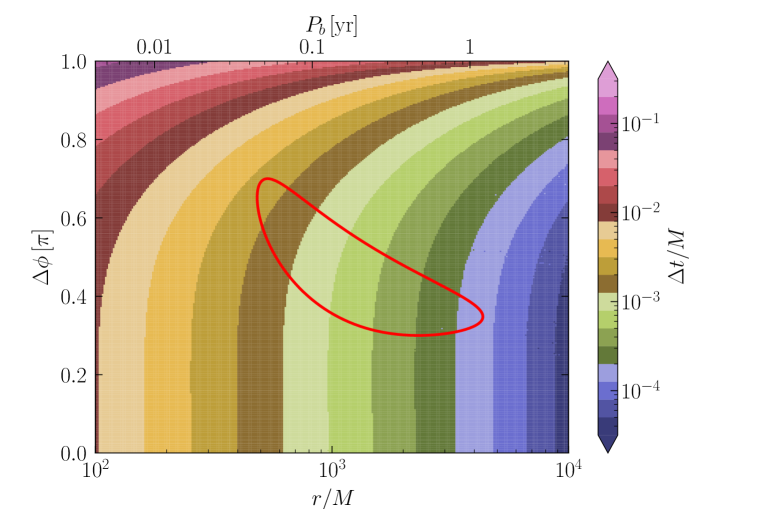
One can directly integrate Eqs. (3.3–3.4) to obtain the light propagation time after getting the impact parameter . In Fig. 1, we plot the time difference between GR and the bumblebee gravity for and as an example. The red line in the figure illustrates a pulsar orbit with an orbital period and an orbital eccentricity . Although this example is somewhat unrealistic for its extremely large , we illustrate it in order to show the deviation from GR clearly. For a pulsar with orbital period around Sgr A*, which has a mass , the typical time difference is , which may be detectable in future observations as the expected timing precision for such a pulsar can reach – ms [6]. The time difference can be even larger if the pulsar is in an orbit with its inclination angle close to or has a large orbital eccentricity. However, this time difference is always proportional at the leading order. For , the time difference is about or less than for pulsars in the interested parameter space, which are hard to be directly detected in the near future. Nevertheless, one still should at least include its leading order effect in the timing model as the residuals caused by this effect might be close to the timing precision, similar to the spirit in the treatment of those next-to-leading order effects in the Double Pulsar [5].
3.2 Orbital motion
As the mass ratio of the pulsar and the Sgr A* BH is smaller than , we will treat the pulsar as a test particle in the BH’s spacetime for the moment. With this assumption, we also neglect the gravitational radiation that causes the decay of orbital period, usually encoded in the parameter. Therefore, the equations of motion for the pulsar read as
| (3.6) | ||||
| (3.7) |
where is the specific energy constant, and is the specific angular momentum constant. By numerically integrating the above equations, one can obtain the orbital motion of the pulsar, as well as the Einstein delay .
As a fiducial case, we study a pulsar with the following orbital parameters,
| (3.8) |
where is the orbital period, is the orbital eccentricity, is the inclination angle, is the longitude of the periastron at , and is the initial orbital phase of the pulsar. As we have ignored the proper motion of Sgr A*, the longitude of the ascending node, , will not affect the TOAs and we choose to fix [47]. The orbital parameters of the pulsar is understood in a Keplerian manner at . For example, the semi-major axis of the orbit is defined through , and the pericenter and apocenter distances are given by and respectively. The relation between the parameters and is determined by the assumption that and are the two roots that result in in Eqs. (3.6–3.7).
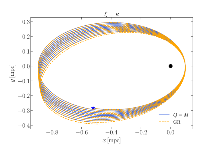
Due to the assumed spherical symmetry of the BH spacetime, the inclination angle is a constant and the motion of the pulsar is in a fixed plane. Figure 2 gives an illustration of the pulsar’s orbits in the orbital plane for GR and the bumblebee gravity with and . The total time span is used, and one can see a secularly increasing deviation between these two orbits. This secular effect corresponds to an additional periastron advance caused by the bumblebee charge. At the leading order of , it reads [31]
| (3.9) |
where is the periastron advance in GR at the first post-Newtonian (PN) level [40]. The leading order effect caused by the bumblebee charge is at the 1 PN level as expected in the parameterized PN (PPN) framework where the PPN parameter for a charged BH in the bumblebee gravity [31]. Compared to its GR counterpart , is suppressed by a factor of and thus becomes much smaller when . However, depending on the value of , this additional periastron advance might be still comparable to the effects caused by the spin of Sgr A*, which is numerically at the 1.5 PN level [48, 6]. Thus it is important in the timing model. Besides the secular effect, we also include all the periodic effects caused by the bumblebee charge by resorting to numerical calculations, although they are in general smaller than the leading order secular effect.
3.3 Leading order effects in
Combining the results of orbital motion and light propagation, one obtains the numerical timing model for the pulsar-SMBH system in the bumblebee gravity. However, as we discussed before, for , it might be unnecessary to calculate all these effects numerically. A leading order approximation should work for the purpose of forecasting the measurability of the bumblebee charge while higher order corrections can be added in real timing models depending on the timing accuracy of the real data.
To construct a timing model with leading order effects in , we adopt the expansion in as well as the usual PN expansion [49], which describes the pulsar’s motion in the harmonic coordinate. The relation between the radial position in the harmonic coordinate and in Eq. (2.1) is described by [31]
| (3.10) |
With the solution derived in Appendix A, one can obtain the relation between and as
| (3.11) |
The leading order correction caused by the bumblebee charge in this relation is at the order of , which will not enter the later calculations as the leading order effects in light propagation and orbital motion are both at the order.
Solving Eqs. (3.3–3.5) to the leading order of and combining the coordinate transformation in Eq. (3.11), one can obtain in the harmonic coordinate
| (3.12) |
where and are the so-called Römer delay and Shapiro delay respectively [40], given by
| (3.13) | ||||
| (3.14) |
and is the additional light propagation delay caused by the bumblebee charge at the leading order
| (3.15) |
Similarly to the leading order Shapiro delay, the leading order expression of diverges at the point , as the leading order calculation is effectively done by integrating along a straight line that will cross the BH when [44]. Here we only include the leading order Shapiro delay, which is at 1 PN order. As including higher-order terms is usually expected to further break the degeneracies between parameters in such a problem, the treatment here is rather conservative. It is sufficient for our purpose here and we leave the problem of constructing a more delicate timing model for future studies.
The orbital motion of a pulsar with leading order corrections of can be calculated analytically using the so-called osculating orbital elements [50] or a similar procedure described by Damour and Deruelle [49]. However, those methods are hard to extend when considering higher order corrections or combining other possible effects such as the BH spin. Simple analytic formula does not exist in general cases. Therefore, we adopt the expansion form of the equations of motion in the harmonic coordinate
| (3.16) |
where points from the central BH to the pulsar, the dots denote time derivatives, , , and . We only keep the 1 PN term and the leading order correction in in this expansion for similar reasons that have been argued before.
The relation between the pulsar’s proper time and the coordinate time has an expansion form as
| (3.17) |
We integrate this equation to obtain the Einstein delay .
After dropping the constant term, one finally has
| (3.18) |
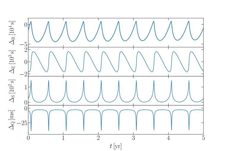
In Fig. 3, we show these time delays for the orbit illustrated before with and . The dominant modification from the bumblebee charge is in the Römer delay at the 1 PN level, due to the additional periastron advance in the bumblebee gravity. The additional propagation time caused by the bumblebee charge has a similar behavior as the Shapiro delay but with an opposite sign, and it is much smaller than the Shapiro delay.
4 Parameter estimation
As a standard procedure for parameter estimation in the pulsar timing process [40, 51], we use the covariance matrix,
| (4.1) |
to estimate the measurement uncertainties of the parameters in the timing model. The log-likelihood function is defined via [40]
| (4.2) | ||||
| (4.3) |
where is the total number of observed TOAs, is the timing precision, is the pulsar rotation number of the -th TOA calculated from the timing model with parameters , and represents the true values of those parameters. We list all the model parameters here
| (4.4) |
As the dependence on only appears in the quadratic form, we choose as the model parameter. Here we treat the coupling constant as a given parameter that describes the gravity model and do not estimate it simultaneously. However, one would have the probability to constrain and simultaneously with high enough timing precision so that the next to leading order effects can be observed. We assume the pulsar spin frequency , corresponding to a normal pulsar, and take the timing precision to be 1 ms in our simulations, which is achievable for future observations [6, 10]. The total observation time is assumed to be 5 years, and TOAs are extracted weekly and uniformly in time, which gives .
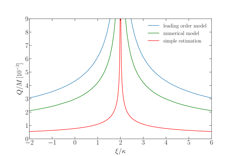
We have constructed a fully numerical timing model and a semi-analytic timing model based on the leading order approximation in Sec. 3. A comparison of the estimation results of the two timing models are shown in Fig. 4. For a pulsar orbit with orbital parameters shown in Eq. (3.8), we present the constraint on as a function of obtained with the two timing models. In the simulation, we assume that GR is correct, which means that the true value of is set to be zero. The constraint on should be understood as an upper limit corresponding to the square root of the uncertainty of . Intuitively, one can estimate upper limits on with , where represents the measurement precision of the periastron advance. For the assumed pulsar-Sgr A* system, can be measured to a precision of [6]. However, this kind of simple estimation is in general too optimistic because the degeneracy between the periastron advance caused by the BH mass and the bumblebee charge leads to larger uncertainties for and when doing a fully global determination of them. Nevertheless, we still plot this simple estimation in Fig. 4 as a rough estimate. From this figure, one can see that the constraints from the leading order model are slightly larger than the constraints from the numerical model, with a factor of about 1.5. This is reasonable as we have ignored all higher order effects of in the leading order timing formula. Therefore, in the following discussion we only present the estimation results obtained from the leading order timing model. One may expect that the results are similar if the fully numerical model were adopted. One also notices that the constraints on are weak when is around as the BH metric reduces to the Schwarzchild solution when [31].
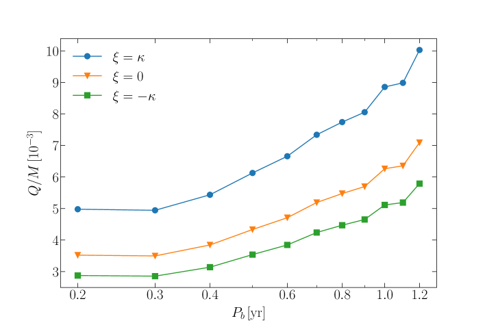
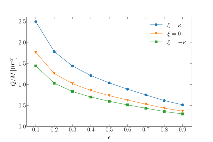
In order to investigate more pulsar-Sgr A* systems than the prototype system in Fig. 4, we vary the orbital parameters. Figure 5 shows the constraints on as functions of the pulsar orbital period for , and . We can see an approximate symmetry with respect to from the leading order metric solution. Therefore, with the constraints on being almost symmetric, we only show the cases. The upper limits for decrease when becomes smaller as both the secular and periodic effects become larger when the pulsar gets closer to the SMBH. We also investigate the influence of the orbital eccentricity and the results are shown in Fig. 6. Compared to the orbital period, a higher orbital eccentricity is relatively more important for constraining the bumblebee charge. This is because that the largest effect caused by the bumblebee charge is the additional periastron advance, which becomes degenerate with the orbital period when the orbital eccentricity is small. For a pulsar with an orbital period of 0.5 yr and an orbital eccentricity of 0.8, one can expect to constrain to when .
5 Discussion
We have explored pulsar-SMBH systems in the bumblebee gravity and discussed possible constraints on the bumblebee charge of Sgr A* by timing a pulsar orbiting around it. We first constructed a timing model based on the fully numerical calculations of the BH metric, light propagation, and pulsar orbital motion in the bumblebee gravity. Considering the future timing precision for such GC pulsars and current constraints on the bumblebee charge of Sgr A* [31, 33], we also constructed a timing model only including the leading order effects based on the expansion solution of the metric that is more efficient and flexible than the fully numerical approach. Our simulation shows that for a pulsar with an orbital period , an orbital eccentricity , a 5-yr observation with weekly recorded TOAs, and a timing precision of 1 ms, one can constrain the bumblebee charge of Sgr A* to be for , which is much better than the current constraints from the EHT observation [33], and at the same order of magnitude as the expected constraint from the extreme-mass-ratio inspiral observation with the Laser Interferometer Space Antenna (LISA) [34].
The limitation of the timing model built here is that we have only considered the static spherical BHs in the bumblebee gravity. For spinning BHs, the spin-orbit coupling and the quadruple moment of the BH both have detectable effects in the pulsar timing observation [48, 6, 8, 16]. Also, the complex environment around Sgr A* perturbs the system [52, 16]. The periastron advance caused by these effects is degenerate with that caused by the bumblebee charge, which brings larger uncertainties in the measurement even though one may separate these effects by considering their periodic effects or combining other observations. Nevertheless, spinning BHs with bumblebee charges might introduce additional features in TOAs that can be used to break the degeneracy. To make a more reliable estimation, one should extend the timing model to include, for example, the spin of Sgr A*. Although complete solutions of arbitrarily rotating BHs in the bumblebee gravity have not been obtained yet, it is still possible to extend the leading order timing model by adding the spin-orbit coupling term in the equations of motion using some specific slowly-rotating BH solutions obtained by Ding and Chen [53]. We leave these kinds of extension for future studies.
Appendix A An analytic solution in orders of
To obtain a solution of Eqs. (2.2–2.4) arranged in the order of , one can start with the expansion
| (A.1) | |||||
| (A.2) | |||||
| (A.3) | |||||
| (A.4) |
where are functions of and is a notation to denote the different orders of . Substituting these equations into the field equations, one can obtain the equations for each order. The expansion for the radius of event horizon is used when applying the boundary conditions.
For a BH with mass and bumblebee charge , we choose the zeroth order solution to be a Schwarzchild solution with mass , i.e.,
| (A.5) | ||||
| (A.6) | ||||
| (A.7) |
Different choices of the zeroth order solution can change the higher order terms but the entire series refer to the same exact solution.
From Eq. (2.2), we obtain the ordinary differential equation for , which reads as
| (A.8) |
The general solution of this equation, , has two integration constants, which can be determined by the two boundary conditions
| (A.9) | |||||
| (A.10) |
Note that the boundary conditions should also be satisfied order by order. Thus one can obtain
| (A.11) |
Then from Eqs. (2.3–2.4) one can derive the ordinary differential equation for , which reads as
| (A.12) |
The general solution is
| (A.13) |
The boundary conditions for come from the requirements that when , and . So one finds . After working out , and can be determined directly from Eq. (2.2) together with respectively.
Repeating the above procedure, one can obtain the solution for a BH with mass and bumblebee charge in orders of . The result up to the order of is listed here
| (A.14) | ||||
| (A.15) | ||||
| (A.16) | ||||
| (A.17) |
The forms of and are chosen such that the RN solution and the Schwarzschild metric can be recovered by the leading order terms at and respectively.
As discussed in Sec. 2, the charged BHs in the bumblebee gravity are indistinguishable with RN BHs in GR at the leading order of . However, this degeneracy can be broken by considering higher order terms as the combination of and changes in the next-to-leading order contributions.
Acknowledgments
This work was supported by the National SKA Program of China (2020SKA0120300), the National Natural Science Foundation of China (11975027, 11991053, 12247128, 11721303), the China Postdoctoral Science Foundation (2021TQ0018), the Max Planck Partner Group Program funded by the Max Planck Society, and the High-Performance Computing Platform of Peking University.
References
- Damour [2009] T. Damour, in Physics of Relativistic Objects in Compact Binaries: From Birth to Coalescence, Vol. 359, edited by M. Colpi, P. Casella, V. Gorini, U. Moschella, and A. Possenti (Springer, Dordrecht, 2009) p. 1, arXiv:0704.0749 [gr-qc] .
- Kramer et al. [2004] M. Kramer, D. C. Backer, J. M. Cordes, T. J. W. Lazio, B. W. Stappers, and S. Johnston, New Astron. Rev. 48, 993 (2004).
- Shao [2023] L. Shao, Lect. Notes Phys. 1017, 385 (2023).
- Hu et al. [2023a] Z. Hu, X. Miao, and L. Shao, (2023a), arXiv:2303.17185 [astro-ph.HE] .
- Kramer et al. [2021] M. Kramer et al., Phys. Rev. X 11, 041050 (2021).
- Liu et al. [2012] K. Liu, N. Wex, M. Kramer, J. M. Cordes, and T. J. W. Lazio, Astrophys. J. 747, 1 (2012).
- Shao et al. [2015] L. Shao et al., in Advancing Astrophysics with the Square Kilometre Array, Vol. AASKA14 (Proceedings of Science, 2015) p. 042, arXiv:1501.00058 [astro-ph.HE] .
- Psaltis et al. [2016] D. Psaltis, N. Wex, and M. Kramer, Astrophys. J. 818, 121 (2016).
- Zhang and Saha [2017] F. Zhang and P. Saha, Astrophys. J. 849, 33 (2017).
- Bower et al. [2018] G. C. Bower et al., ASP Conf. Ser. 517, 793 (2018), arXiv:1810.06623 [astro-ph.HE] .
- Weltman et al. [2020] A. Weltman et al., Publ. Astron. Soc. Austral. 37, e002 (2020), arXiv:1810.02680 [astro-ph.CO] .
- Bower et al. [2019] G. C. Bower et al., Bull. Am. Astron. Soc. 51, 438 (2019).
- Goddi et al. [2019] C. Goddi et al. (EHT), The Messenger 177, 25 (2019), arXiv:1910.10193 [astro-ph.HE] .
- Dong et al. [2022] Y. Dong, L. Shao, Z. Hu, X. Miao, and Z. Wang, JCAP 11, 051 (2022).
- Akiyama et al. [2022] K. Akiyama et al. (Event Horizon Telescope), Astrophys. J. Lett. 930, L17 (2022), arXiv:2311.09484 [astro-ph.HE] .
- Hu et al. [2023b] Z. Hu, L. Shao, and F. Zhang, (2023b), arXiv:2312.01889 [astro-ph.HE] .
- Paumard et al. [2006] T. Paumard et al., Astrophys. J. 643, 1011 (2006).
- Lu et al. [2013] J. R. Lu, T. Do, A. M. Ghez, M. R. Morris, S. Yelda, and K. Matthews, Astrophys. J. 764, 155 (2013).
- Wharton et al. [2012] R. S. Wharton, S. Chatterjee, J. M. Cordes, J. S. Deneva, and T. J. W. Lazio, Astrophys. J. 753, 108 (2012).
- Eatough et al. [2013] R. P. Eatough et al., Nature 501, 391 (2013).
- Abbate et al. [2023] F. Abbate et al., Mon. Not. Roy. Astron. Soc. 524, 2966 (2023), arXiv:2307.03230 [astro-ph.HE] .
- Kramer et al. [2000] M. Kramer, B. Klein, D. R. Lorimer, P. Mueller, A. Jessner, and R. Wielebinski, ASP Conf. Ser. 202, 37 (2000), arXiv:astro-ph/0002117 .
- Siemion et al. [2013] A. Siemion et al., in Neutron Stars and Pulsars: Challenges and Opportunities after 80 years, Vol. 291, edited by J. van Leeuwen (2013) pp. 57–57.
- Liu et al. [2021] K. Liu et al., Astrophys. J. 914, 30 (2021).
- Torne et al. [2023] P. Torne et al. (EHT), (2023), arXiv:2308.15381 [astro-ph.HE] .
- Shao et al. [2020] L. Shao, N. Wex, and S.-Y. Zhou, Phys. Rev. D 102, 024069 (2020), arXiv:2007.04531 [gr-qc] .
- Eatough et al. [2023] R. P. Eatough et al., in 15th Marcel Grossmann Meeting on Recent Developments in Theoretical and Experimental General Relativity, Astrophysics, and Relativistic Field Theories (2023) arXiv:2306.01496 [astro-ph.HE] .
- Kostelecky [2004] V. A. Kostelecky, Phys. Rev. D 69, 105009 (2004).
- Bluhm and Kostelecky [2005] R. Bluhm and V. A. Kostelecky, Phys. Rev. D 71, 065008 (2005).
- Liang et al. [2022] D. Liang, R. Xu, X. Lu, and L. Shao, Phys. Rev. D 106, 124019 (2022).
- Xu et al. [2023a] R. Xu, D. Liang, and L. Shao, Phys. Rev. D 107, 024011 (2023a).
- Hellings and Nordtvedt [1973] R. W. Hellings and K. Nordtvedt, Phys. Rev. D 7, 3593 (1973).
- Xu et al. [2023b] R. Xu, D. Liang, and L. Shao, Astrophys. J. 945, 148 (2023b).
- Liang et al. [2023] D. Liang, R. Xu, Z.-F. Mai, and L. Shao, Phys. Rev. D 107, 044053 (2023).
- Heisenberg et al. [2017] L. Heisenberg, R. Kase, M. Minamitsuji, and S. Tsujikawa, JCAP 08, 024 (2017).
- Cisterna et al. [2016] A. Cisterna, M. Hassaine, J. Oliva, and M. Rinaldi, Phys. Rev. D 94, 104039 (2016).
- Babichev et al. [2017] E. Babichev, C. Charmousis, and A. Lehébel, JCAP 04, 027 (2017).
- Barausse and Sotiriou [2008] E. Barausse and T. P. Sotiriou, Phys. Rev. Lett. 101, 099001 (2008), arXiv:0803.3433 [gr-qc] .
- Mai et al. [2023] Z.-F. Mai, R. Xu, D. Liang, and L. Shao, Phys. Rev. D 108, 024004 (2023).
- Damour and Deruelle [1986] T. Damour and N. Deruelle, Ann. Inst. Henri Poincaré Phys. Théor. 44, 263 (1986).
- Damour and Taylor [1992] T. Damour and J. H. Taylor, Phys. Rev. D 45, 1840 (1992).
- Lorimer and Kramer [2005] D. R. Lorimer and M. Kramer, Handbook of Pulsar Astronomy (Cambridge University Press, Cambridge, England, 2005).
- Reid and Brunthaler [2004] M. J. Reid and A. Brunthaler, Astrophys. J. 616, 872 (2004).
- Klioner and Zschocke [2010] S. A. Klioner and S. Zschocke, Class. Quant. Grav. 27, 159801 (2010).
- Della Monica et al. [2023] R. Della Monica, I. de Martino, and M. de Laurentis, Mon. Not. Roy. Astron. Soc. 524, 3782 (2023).
- Lai and Rafikov [2005] D. Lai and R. R. Rafikov, Astrophys. J. Lett. 621, L41 (2005).
- Taylor [1994] J. H. Taylor, Rev. Mod. Phys. 66, 711 (1994).
- Wex and Kopeikin [1999] N. Wex and S. Kopeikin, Astrophys. J. 514, 388 (1999).
- Damour and Deruelle [1985] T. Damour and N. Deruelle, Ann. Inst. Henri Poincaré Phys. Théor. 43, 107 (1985).
- Poisson and Will [2014] E. Poisson and C. M. Will, Gravity: Newtonian, Post-Newtonian, Relativistic (Cambridge University Press, 2014).
- Hobbs et al. [2006] G. Hobbs, R. Edwards, and R. Manchester, Mon. Not. Roy. Astron. Soc. 369, 655 (2006).
- Merritt et al. [2010] D. Merritt, T. Alexander, S. Mikkola, and C. M. Will, Phys. Rev. D 81, 062002 (2010).
- Ding and Chen [2021] C. Ding and X. Chen, Chin. Phys. C 45, 025106 (2021), arXiv:2008.10474 [gr-qc] .