(cvpr) Package cvpr Warning: Single column document - CVPR requires papers to have two-column layout. Please load document class ‘article’ with ‘twocolumn’ option mj

Differentiable Point-based Inverse Rendering
Supplementary Information

This document offers extended information and further results of DPIR, complementing the main paper.

1 Network Architecture

Figure 1 shows the overall structure of of our DPIR network architecture which consists of four MLPs: (a) geometry network $\Theta_{\text{SDF}}$, (b) diffuse albedo network $\Theta_{d}$, (c) specular basis coefficient network $\Theta_{c}$, (d) specular basis network $\Theta_{s}$.

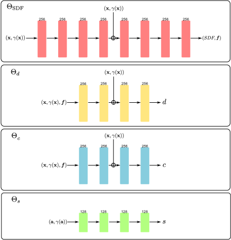
Figure 1: Network architecture. To compute point radiance, we estimate surface normal, diffuse albedo, and specularity using MLPs. Here, each block represents the fully-connected layer with its size of the hidden channel written at the top of the block. We use Softplus activation layer for $\Theta_{\text{SDF}}$ and ReLU activation layer for the other networks. $\oplus$ denotes skip connection that concatenates its output features with the input.

1.1 Geometry Network

We use 8-layer MLPs of width 256 for SDF values and geometric features with skip connection at the 4th layer. We add positional encoding for input 3D point position $\mathbf{x}$ using 6 frequency components to train high frequency information. Positional encoding for point location $\mathbf{x}$ is represented as $\gamma(\mathbf{x})$.

1.2 Diffuse Albedo Network

We use 4-layer MLPs of width 256 for diffuse albedo with skip connection at the 2nd layer. We add positional encoding for input 3D point position $\mathbf{x}$ using 10 frequency components. Diffuse albedo network also utilizes SDF-based geometric features as input concatenated with positional-encoded point location.

1.3 Specular Basis Coefficient Network

We use the same network architecture with diffuse albedo network. Specular basis coefficient network outputs 1 channel regularized values which are combinated with specular bases to compute specularity.

1.4 Specular Basis Network

We use 4-layer MLPs of width 128 for specular basis without skip connection. We compute SDF normal of each point and calculate half-way vector $\boldsymbol{h}$ considering viewing direction and light direction. We can represent isotropic BRDF with two parameters $(\theta_{h},\theta_{d})$ following  [1, 2], where $\theta_{h}=arccos(\mathbf{n}^{T}\mathbf{h})$, $\theta_{d}=arccos(\mathbf{v}^{T}\mathbf{h})$. We take the cosine value of these values and add positional encoding for two variables using 4 frequency components. Positional encoding for half-angle vectors $\mathbf{a}$ is represented as $\gamma(\mathbf{a})$.

2 Loss Functions

We optimize point positions $\mathbf{x}$, point radii $r$, and MLPs for SDF $\Theta_{\text{SDF}}$, diffuse albedo $\Theta_{d}$, specular coefficient $\Theta_{c}$, and specular-basis $\Theta_{s}$ by minimizing the following loss function:

$$\mathcal{L}_{2}+\lambda_{\mathrm{ssim}}\mathcal{L}_{\mathrm{ssim}}+\lambda_{\mathrm{SDF}}\mathcal{L}_{\mathrm{SDF}}+\lambda_{\mathrm{c}}\mathcal{L}_{\mathrm{c}}+\lambda_{\mathrm{m}}\mathcal{L}_{\mathrm{m}}.$$ (1)

Here, $\mathcal{L}_{2}$ is the $\mathbf{l}_{2}$ loss for the reconstructed image $I^{{}^{\prime}}$ and the observed image $I$. $\mathcal{L}_{\mathrm{ssim}}$ is the differentiable SSIM loss which considers luminance, contrast, structure for $I^{{}^{\prime}}$ and $I$. Our fast splatting-based forward rendering allows DPIR to utilize SSIM loss, which is often omitted in other rendering methods due to its long computation time, resulting better reconstruction quality. $\mathcal{L}_{\mathrm{SDF}}$ is to promote the zero-level set of SDF exists near explicit point positions, combining discrete point representation with continuous SDF. $\mathcal{L}_{\mathrm{c}}$ regularizes $\mathbf{l}_{1}$ norm of estimated per-point specular coefficients to be $\epsilon$. Specular coefficients are constrained to be positive and under $\epsilon$. $\mathcal{L}_{\mathrm{m}}$ is the $\mathbf{l}_{2}$ loss for the reconstructed mask and the ground truth mask. Reconstructed mask image is rendered by point-based splatting with radiance of 1 for all points. We set $\lambda_{\mathrm{ssim}}$, $\lambda_{\mathrm{SDF}}$, $\lambda_{\mathrm{c}}$ and $\lambda_{\mathrm{m}}$ as 0.2, 1.0, 0.1 and 0.1, respectively.

3 Optimization Techniques

3.1 Mask-based Point Initialization

For point cloud initialization, we employ rejection sampling method which samples 3D points uniformly, project these points on each image plane, and let them fall within all the masks [5]. Mask-based point initialization provides coarse geometry for efficient and stable optimization, thus DPIR reconstruction quality is dependent on the accuracy of the mask inputs. We show ablation study that mask inputs improves reconstruction quality while DPIR can obtain plausible reconstruction result without mask.

3.2 Coarse-to-fine Updates

Our method adopts coarse-to-fine updates to learn accurate point cloud representations for geometry and reflectance. First, we employ a voxel discretization to combine points within same voxel into one single point. Second, we compute the distances between aggregated points and standard deviation of these distances. We then remove outliers whose standard deviation is beyond threshold. Voxel-based downsampling enables pruning of superfluous points. After we prune unnecessary points, we insert new points into the point cloud by upsampling remained point representations with same parameters. We repeat these stages for 5 times to achieve coarse-to-fine updates with stable and fast training. Both of mask-based initialization and coarse-to-fine updates are inspired by  [5].

3.3 Training

To train our DPIR method, we empirically choose sampling rate of the number of initialized points and the initialized point radius considering the size of each object. We train 40 epochs for every stage and do not consider visibility at the first stage. Our DPIR method is trained for 7 stages which take 2 hours to converge. We use Adam as optimizer and set the initial learning rate for the point parameters and network parameters as 1e-4 and 5e-4, respectively. Both of learning rates are decayed exponentially for every epoch with a factor of 0.93. We use PyTorch and test DPIR on a single NVIDIA RTX 3090 GPU.

4 Dataset

4.1 DiLiGenT-MV

We test our DPIR method on DiLiGenT-MV, multi-view multi-light image dataset which is often used for evaluating multi-view photometric stereo. DiLiGenT-MV dataset consists of 5 objects, called Bear, Buddha, Cow, Pot2, Reading. For each object, images are captured under horizontally rotated 20 cameras with same angle and same elevation. For each view, 96 images are captured under different single directional light source with different light intensity. We preprocessed images to make low intensity images brighter by normalizing images according to the ground truth light intensity. We also cropped the original images with 612 $\times$ 512 into 400 $\times$ 400 to remove empty background region for efficiency. Our pre-processed dataset followed the instructions from PS-NeRF [3].

4.2 Synthetic Photometric Dataset

We also test our DPIR method on synthetic photometric dataset, following the configuration of mobile flash photography  [4]. We rendered 4 objects, called Dragon, Head, Horse, Maneki, with Blender using mesh and image texture data from IRON [4]. We rendered 300 views images with co-located point lights and used 200/100 views for training/testing, respectively. It took around 3 hours to render ground truth images and normal for 300 views.

5 Additional Ablation Study

	Multi-view multi-light dataset				Photometric dataset
Method	PSNR $\uparrow$	SSIM $\uparrow$	LPIPS $\downarrow$	MAE $\downarrow$	PSNR $\uparrow$	SSIM $\uparrow$	LPIPS $\downarrow$	MAE $\downarrow$
Proposed	36.73	0.9822	0.0091	7.16	35.56	0.9734	0.0285	8.74
w/o vis	35.17	0.9756	0.0126	9.57	x	x	x	x
w/o SDF	33.39	0.9704	0.0156	21.89	34.55	0.9655	0.0378	19.42
w/o radii	26.62	0.9616	0.0392	10.48	35.48	0.9740	0.0295	8.77
w/o $\mathcal{L}_{\mathrm{ssim}}$	32.97	0.9738	0.0132	9.01	34.75	0.9718	0.0373	10.32
basis 1	36.12	0.9816	0.0096	7.41	35.12	0.9712	0.0303	9.31
basis 5	36.44	0.9820	0.0094	7.22	35.45	0.9731	0.0287	8.76
basis 13	36.40	0.9821	0.0092	7.11	35.41	0.9732	0.0283	8.77

Table 1: Quantitative comparison of ablation studies for multi-view multi-light dataset and photometric dataset.

5.1 Point-based Shadow Detection

We evaluate the importance of the point-based visibility test of DPIR. Note that visibility of every point is set to 1 on photometric dataset as the light source and the camera are co-located. Table 1 shows that point-based shadow detection method improves both image and normal reconstruction quality. Especially, normal estimation of self-occluded region is enhanced.

5.2 Hybrid Shape Representation

We evaluate the impact of hybrid point-volumetric shape representation. Table 1 shows that using only point representation and per point normal for inverse rendering recurs inaccurate reconstruction. Our hybrid point-volumetric representation improves normal reconstruction quality by sampling surface normals of discrete points from continuous SDF

5.3 Dynamic Point Radius

We evaluate the impact of point radius optimization. Table 1 shows that learning not only the point position but also point radius enables accurate geometry reconstruction for low and high frequency details. Dynamic point radius shows reconstruction improvement of large margin especially on multi-view multi-light dataset.

5.4 Number of Basis

We evaluate the impact of the number of specular basis. Table 1 and Figure 2 show that using 9 bases provides a converged accuracy in a tested scene. Using few specular basis such as one and five results in inaccurate reconstructions. The number of specular basis is related to the representation power of specularity and normal.

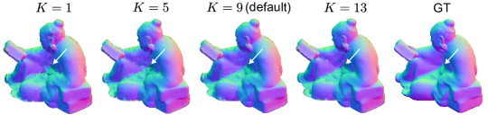
Figure 2: Impact of the number of specular basis. Increasing the number of specular basis improves reconstruction quality and here using nine bases shows converged performance.

5.5 Impact of SSIM Loss

We evaluate the importance of SSIM loss which is computationally expensive. Our DPIR method adopts SSIM loss for better reconstruction based on fast splatting-based rendering. It requires 0.15$\times$ additional training time, while improving image and normal reconstruction quality for a large margin.

5.6 Number of Training Views and Lights

Table 2 shows the normal reconstruction accuracy with varying number of training views and lightings. We found that the number of views plays an important role while the light gives a smaller impact when the number of training lights exceeds 16. Our method can achieve state-of-the-art reconstruction result when trained with only 16 lights.

	4 Lightings	10 Lightings	16 Lightings	30 Lightings
5 Views	22.78	18.89	17.02	15.53
10 Views	19.04	13.69	11.53	10.05
15 Views	14.63	10.15	8.88	8.22

Table 2: Impact of the number of views and lightings for ”Reading”, in terms of normal reconstruction with MAE.

5.7 Mask Dependency

DPIR utilizes mask inputs for point location initialization and mask loss. Our method often achieves plausible reconstruction results even without masks inputs which show the potential applicability of DPIR for larger-scale scene. For complex geometry object, our point locations diverge as shown in Figure 3, meaning our optimization techniques are incomplete. Developing our optimization techniques for complex scene without mask inputs is our future work.

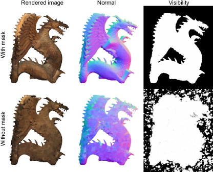
Figure 3: Importance of mask inputs. We test our DPIR without mask inputs, initializing point positions with randomly sampled points inside unit sphere. For complex scene as ”Dragon”, point positions are noisy and diverge.

6 Additional Discussions

6.1 Specular Basis BRDFs and Specular Coefficients

We utilize regularized basis BRDF representation to estimate accurate spatially-varying BRDFs from limited light-view angular samples. Figure. 4 shows visualization of spatially-varying BRDFs, specular basis BRDFs, and specular coefficients of ”Cow”. Specular basis BRDFs for gold appearance have high specular coefficients for body region. Specular basis BRDFs for silver appearance have high specular coefficients for horn region. Specular coefficients for diffuse dominant region as red and yellow have low intensity of specular basis BRDFs.

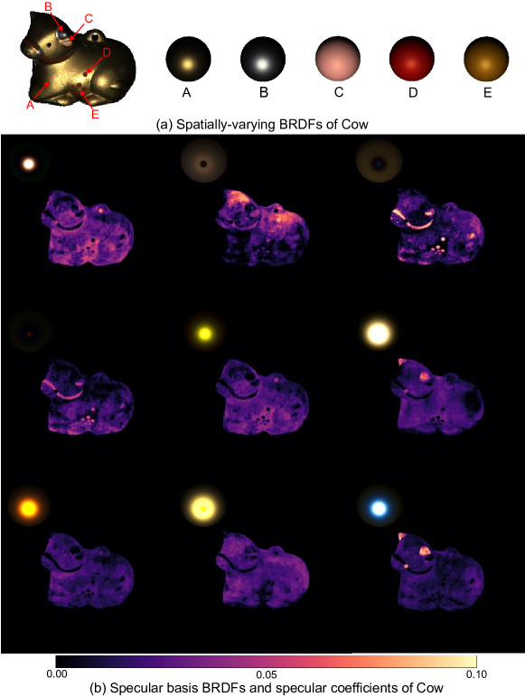
Figure 4: Estimated spatially-varying BRDFs, specular basis BRDFs, and specular coefficients. We visualize the BRDFs on unit spheres illuminated by a point light source. (a) shows spatially-varying BRDFs of ”Cow” with diverse appearance. (b) shows specular basis BRDFs and corresponding specular coefficients.

6.2 Evaluation Metrics with Mask

For fair quantitative comparison between different baselines, mask computation performs critically especially on the mean angular error (MAE). We used rendered mask region for calculating the MAE, while mask estimation of each baseline is different with ground-truth mask. We calculate the MAE with rendered normal and ground-truth normal using rendered mask. Image reconstruction metrics (PSNR, SSIM, LPIPS) are calculated with white background images.

6.3 Specularity with Shading

We visualize specularity image with shading which denotes cosine value between normal and light direction. Our DPIR method computes the point radiance with point BRDF and shading. Thus, we render specularity image by computing point radiance consisting of specular BRDF and shading. Figure. 5 shows ablation study with shading.

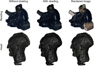
Figure 5: Specularity images with and without shading. Specularity images without shading have more artifacts at the edge of the object, while specularities are more stable with shading.

7 Additional Results

7.1 Environment Map Relighting

Our DPIR method allows environment map relighting by integrating reflected radiance for each light source in the environment map. In Fig. 6, ”Bear”, ”Buddha”, ”Cow”, ”Pot2” and ”Reading” are rendered with different environment map. They show faithful relighting results based on the environment map.

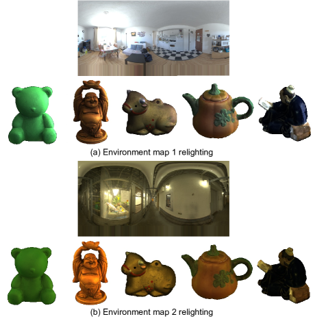
Figure 6: Environment map rendering. We render various objects with two environment maps. Both of rendering results show faithful relighting by reconstructed surface normals, spatially varying BRDFs, and visibility.

7.2 Additional Results with Multi-view Multi-light Dataset

Figure 7 shows visualization of all objects from DiLiGenT-MV dataset. Our DPIR method achieves the best shape and material reconstruction results with multi-view multi-light dataset. Hence, we provide the visualization of the rendered image, estimated normal, diffuse albedo, specularity, visibility, and depth map. It demonstrates that our method is robust to diverse shapes and materials in real-world objects. Figure 8 shows novel view relighting of 5 view points and 8 light directions.

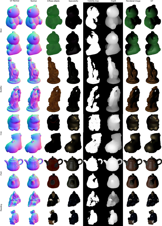
Figure 7: Reconstruction results of DiLiGenT-MV objects. We visualize rendered image, normal, diffuse albedo, specularity, visibility map, depth map with ground-truth normal and image. We perform novel-view relighting with various view points and lightings. In ”Bear”, the object has smooth surface, and visibility maps are well estimated with point-based shadow detection. ”Buddha” has complex geometry and produces self-occlusion at head region. In ”Cow”, the object consists of metal and has difficulty in reconstructing eye region. In ”Pot2”, high frequency details are well reconstructed such as top and leaf of the object. ”Reading” has concave geometry and produces high specular effects. Our DPIR method shows high quality surface and material reconstruction. We scale ”Cow” and ”Pot2” images brighter using gamma

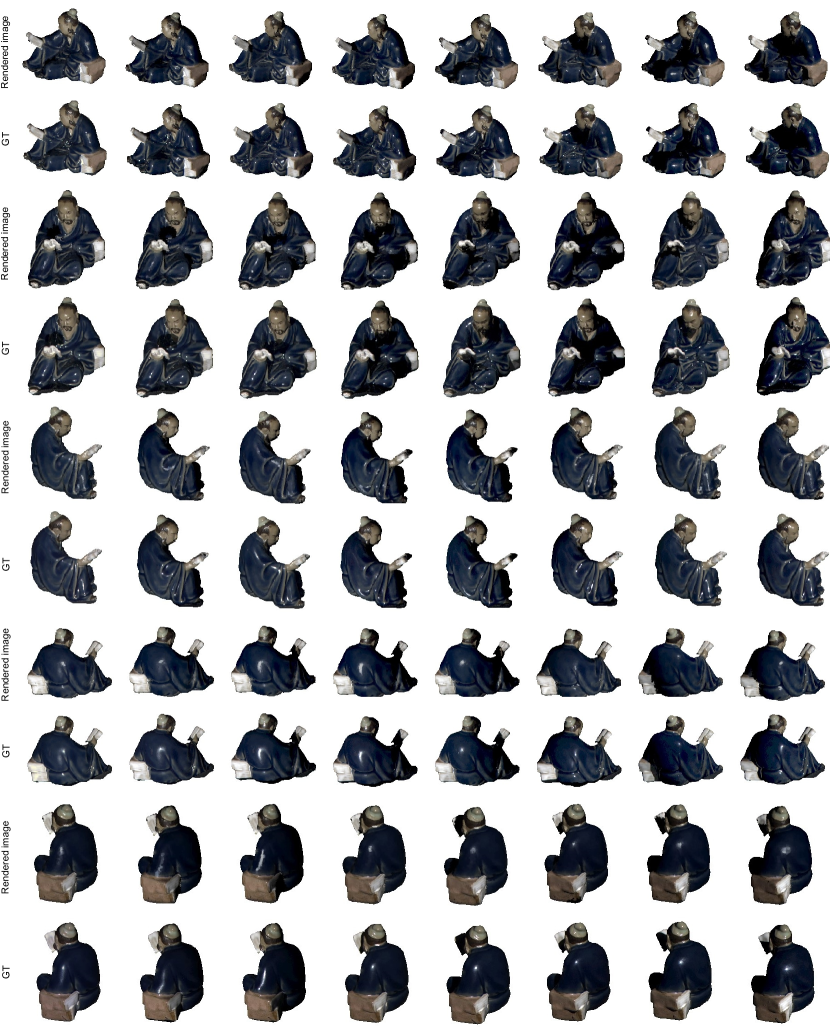
Figure 8: Novel view relighting. We visualize rendered images of 5 novel view points and 8 novel light sources. Our DPIR method achieves faithful reconstruction of shape and material for untrained scene. We scale up reconstructed images and ground-truth images for visualization.

7.3 Additional Results with Photometric Dataset

Figure 9 shows visualization of all objects from synthetic photometric dataset. Our DPIR method achieves the state-of-the-art reconstruction results on different views with co-located point lights. Both of evaluations with different datasets demonstrate that our method is applicable to diverse illumination settings with flexible number of view points. Small number of view points can be compensated by the number of illuminations.

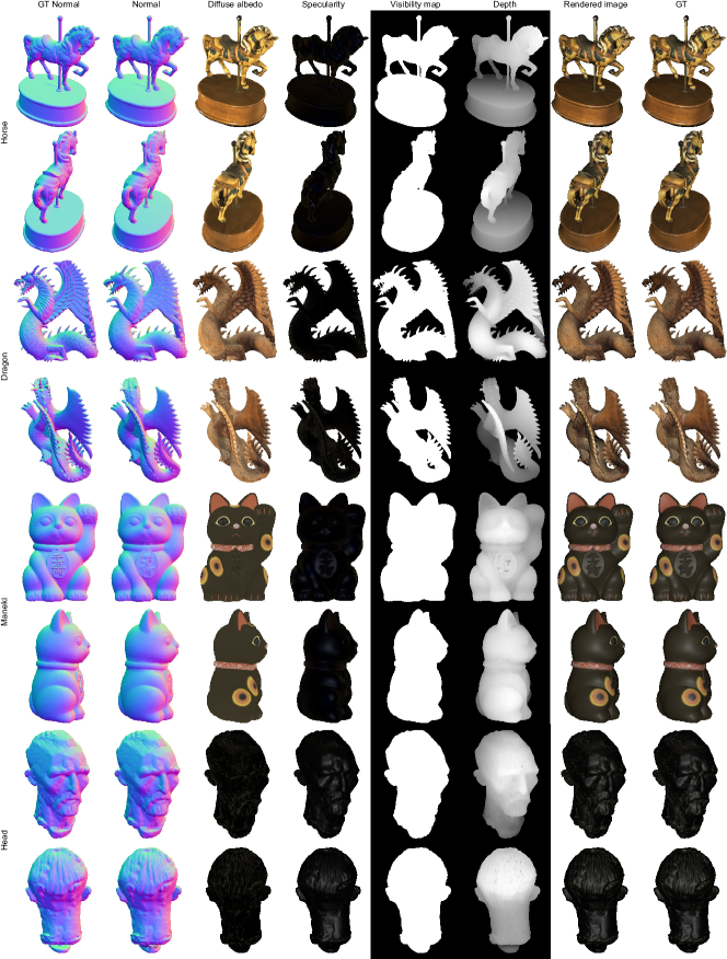
Figure 9: Reconstruction results of photometric dataset. We perform novel-view relighting on various view points with co-located point lights.

References

- [1] Jason Lawrence, Szymon Rusinkiewicz, and Ravi Ramamoorthi. Efficient brdf importance sampling using a factored representation. ACM Trans. Graph., 23(3):496–505, 2004.
- [2] Junxuan Li and Hongdong Li. Neural reflectance for shape recovery with shadow handling. In IEEE Conf. Comput. Vis. Pattern Recog., pages 16221–16230, 2022.
- [3] Wenqi Yang, Guanying Chen, Chaofeng Chen, Zhenfang Chen, and Kwan-Yee K Wong. Ps-nerf: Neural inverse rendering for multi-view photometric stereo. In Eur. Conf. Comput. Vis., pages 266–284. Springer, 2022.
- [4] Kai Zhang, Fujun Luan, Zhengqi Li, and Noah Snavely. Iron: Inverse rendering by optimizing neural sdfs and materials from photometric images. In IEEE Conf. Comput. Vis. Pattern Recog., pages 5565–5574, 2022.
- [5] Qiang Zhang, Seung-Hwan Baek, Szymon Rusinkiewicz, and Felix Heide. Differentiable point-based radiance fields for efficient view synthesis. In SIGGRAPH Asia 2022 Conference Papers, pages 1–12, 2022.