Average-Case Dimensionality Reduction in $\ell_{1}$: Tree Ising Models

Given an arbitrary set of high dimensional points in $\ell_{1}$, there are known negative results that preclude the possibility of mapping them to a low dimensional $\ell_{1}$ space while preserving distances with small multiplicative distortion. This is in stark contrast with dimension reduction in Euclidean space ($\ell_{2}$) where such mappings are always possible. While the first non-trivial lower bounds for $\ell_{1}$ dimension reduction were established almost 20 years ago, there has been minimal progress in understanding what sets of points in $\ell_{1}$ are conducive to a low-dimensional mapping.

In this work, we shift the focus from the worst-case setting and initiate the study of a characterization of $\ell_{1}$ metrics that are conducive to dimension reduction in $\ell_{1}$. Our characterization focuses on metrics that are defined by the disagreement of binary variables over a probability distribution -- any $\ell_{1}$ metric can be represented in this form. We show that, for configurations of $n$ points in $\ell_{1}$ obtained from tree Ising models, we can reduce dimension to $\mathrm{polylog}(n)$ with constant distortion. In doing so, we develop technical tools for embedding capped metrics (also known as truncated metrics) which have been studied because of their applications in computer vision, and are objects of independent interest in metric geometry.

1 Introduction

Given an arbitrary set of $n$ high dimensional points in $\ell_{1}$, we know that it is impossible to map them to a low dimensional $\ell_{1}$ space while preserving distances with small multiplicative distortion. Known lower bounds [BC05, LN04, ACNN11, Reg13] show that for any desired distortion $c$, at least $n^{\Omega(1/c^{2})}$ dimensions are needed. This is in stark contrast with dimension reduction in Euclidean space ($\ell_{2}$) where mappings to $O(\log(n))$ dimensions are possible with $1+\varepsilon$ distortion. While these results rule out dimension reduction for arbitrary sets of point in $\ell_{1}$, a natural question is: Are there broad families of structured sets of points in $\ell_{1}$ that admit low dimensional mappings with small distortion? Despite the fact that strong lower bounds for $\ell_{1}$ dimension reduction were established almost 20 years ago, there has been little progress in understanding this question.

In this work, we shift the focus from the worst-case setting and initiate the study of a characterization of $\ell_{1}$ metrics that admit low-dimensional $\ell_{1}$ representations. Our starting point is that any $\ell_{1}$ metric can be represented by the disagreement of binary variables over a probability distribution $D$ -- a simple consequence of the fact that any $\ell_{1}$ metric can be embedded into the (possibly infinite-dimensional) Hamming cube. This distribution viewpoint of $\ell_{1}$ metrics leads to a natural reframing of the earlier question: What classes of distributions $D$ lead to $\ell_{1}$ metrics that admit low distortion, low dimensional $\ell_{1}$ embeddings?

We initiate a study of this question and show that, for configurations of $n$ points in $\ell_{1}$ obtained from tree Ising models, we can reduce dimension to $\mathrm{polylog}(n)$ with constant distortion. Tree Ising models are natural candidates for distributions to study in this context. One the one hand, they have been studied extensively in the recent theoretical computer science literature on testing and learning [DP21, BGPV21, BABK22, KDDC23]. On the other hand, it is well known that tree metrics embed isometrically into $\ell_{1}$ and the question of $\ell_{1}$ dimension reduction for tree metrics has been studied in the literature [CS02, LdMM13, LM13]. We should note, however, that the metrics that arise from tree Ising models are not tree metrics themselves -- establishing that they admit low dimensional $\ell_{1}$ embeddings is subtle and non-trivial.

In order to establish our results, we develop technical tools for embedding capped metrics (also known as truncated metrics in the literature). Truncated metrics arise in image segmentation in computer vision [BVZ98, IG98, KVT11, Kum14, KD16, PPK17] and have been studied in theoretical computer science in the context of the metric labeling problem motivated by this application [GT00, CKNZ04, KKMR06]; they are also objects of independent interest in metric geometry, where they have been studied in the context of metric dimension [JO12, BRV16, TFL21, TFL23], including very recent work on the metric dimension of truncated tree metrics [BKR23, GY23].

While our work shows that $\ell_{1}$ metrics represented by tree Ising models allow for low dimensional embeddings, it would be interesting to see how far this program can be extended -- namely, is there a more general class of graphical models (e.g., having bounded treewidth) that also allow for low dimensional embeddings in $\ell_{1}$? We discuss this in more detail in Section 7, where we show that even Bayesian networks with treewidth-3 capture the lower bound of [CS02], precluding the possibility of embedding them in $n^{o(1)}$ dimensions. This suggests that tree Ising models are near the boundary of families of graphical models representing $\ell_{1}$ metrics that admit low dimensional embeddings. We also detail classes of graphical models for which this question remains open.

Related Work:

The study of dimension reduction in metric spaces has a rich history (see the survey [Nao18]). Dimension reduction for $\ell_{1}$ has been studied in several contexts: the performance of linear embeddings on structured subsets[CS02, BGI⁺08, AORP10, Rac16, KW16, Jac17, Lot19] as well as nearest neighbor preserving embeddings -- a weaker requirement than low distortion (i.e. bilipschitz) embeddings [IN07, EMP19]. The lower bounds for $\ell_{1}$ dimension reduction have been generalized to the nuclear norm [NPS20, RV20].

The question of characterizing metrics that embed into constant dimensional $\ell_{2}$ (and $\ell_{p}$ for $p>2$) in terms of the doubling dimension has received considerable attention in the literature. A major open problem in this space is to determine whether doubling metrics embed into $\ell_{2}$ with constant dimensions and constant distortion [LP01, GKL03, LN14, BGN15, LDRW18, Tao20, BSS21].

Similar in spirit to our study of structured subsets of $\ell_{1}$ that admit low dimensional, low distortion $\ell_{1}$ representations, is the study of graph metrics that embed into $\ell_{1}$ with constant distortion. A well-known open problem here is to determine whether graph metrics from minor-closed families (e.g. planar graphs) embed into $\ell_{1}$ with constant distortion [GNRS04, Rao99, CGN⁺06, LS09, LS13, Sid13, KLR19, Fil20, Kum22].

Several other notions of dimension reduction are well studied in the literature. See [B⁺10, CG15, BFN19, DHK⁺21]. Somewhat related to (but different from) the focus of this work is the question of approximating distance metrics on probability distributions with short vectors [AKM⁺16, CGV16, Mel19].

2 Overview of Results

In the context of understanding the classes of distributions that are amenable to low-dimensional $\ell_{1}$ embeddings, our main result shows that it is possible to embed distance metrics over Tree Ising models:

Theorem 1 (Embedding Tree Ising Models).

Any distance metric over tree Ising models (i.e, $d_{D}(i,j)=c\cdot\operatorname{{Pr}}_{X\sim D}[X_{i}\neq X_{j}]$, where $D$ is a tree Ising model distribution on $n$ random variables $X_{1},\dots,X_{n}$) can be embedded into $(\mathds{R}^{O(\log^{2}(n))},\ell_{1})$ with $\Theta(1)$ distortion.

This proof follows two primary thrusts. First, in Section 5.2 we characterize that distance metrics corresponding to tree Ising models can approximately have distances between $X_{i},X_{j}$ decomposed into three sources:

• The difference in the marginals between $X_{i},X_{j}$, or $|\operatorname{{Pr}}[X_{i}=0]-\operatorname{{Pr}}[X_{j}=0]|$.

• The amount of independence between $X_{i}$ and $X_{j}$, which we formalize by a notion called ‘‘Bernoulli randomness’’ in Section 5.1. This simply-defined quantity behaves intuitively similar to Shannon entropy in how it measures randomness, yet has smoothness that makes it more amenable to the $\ell_{1}$ setting.

• The strength of any negative correlation between $X_{i}$ and $X_{j}$.

Most interestingly, we now sketch how to embed distance originating from the ‘‘independence’’ between two variables $X_{i}$ and $X_{j}$. For simplicity, suppose that the other two sources of distance are zero for $X_{i}$ and $X_{j}$ (meaning, their marginals are the same and they are not negatively correlated). Then, one could roughly view the joint distribution over the $X_{i},X_{j}$ by some process where first $X_{i}$ is realized, then with probability $p$ we sample $X_{j}$ independently, and with probability $1-p$ we set $X_{j}=X_{i}$. The parameter $p$ roughly corresponds to the independence between $X_{i}$ and $X_{j}$: if $p=0$ then they are completely dependent, and if $p=1$ they are completely independent. In this setting, we find that the distance metric $\operatorname{{Pr}}_{D}[X_{i}\neq X_{j}]$ is roughly equal to $\Theta(1)\cdot p\cdot M(x_{i})$, where $M(x_{i})=\min(\operatorname{{Pr}}[X_{i}=0],\operatorname{{Pr}}[X_{i}=1])$ is a quantity that measures how far $X_{i}$ is from being completely deterministic (i.e. biased towards one value). We later determine a weight $w_{e}$ for each edge in the tree (in terms of ‘‘Bernoulli randomness’’), such that, in this setting, if we were to think of the path connecting $X_{i}$ and $X_{j}$, $\operatorname{{Pr}}_{D}[X_{i}\neq X_{j}]\approx\min(\sum_{e:i\rightarrow j}w_{e},M(x_{i}))$. One interpretation of this is that independence can accumulate along a path in the tree, but at some point the effect of independence is capped by the amount of randomness in the marginals of $X_{i},X_{j}$. We are able to generalize the usage of this idea, to reduce the task of embedding tree Ising models into $\ell_{1}$ to the task of embedding a ‘‘capped’’ tree metric, where $d(x_{i},x_{j})=\min(\sum_{e:i\rightarrow j}w_{e},\max(M(x_{i}),M(x_{j}))$. Here, $M(x_{i}),M(x_{j})$ are ‘‘caps’’ for each vertex, which, in the context of tree Ising models, ultimately end up being related to the biases of the variables. Crucially, our caps satisfy a Lipschitz property $|M(x_{i})-M(x_{j})|\leq d(x_{i},x_{j})$. Our second thrust shows that we can embed this new metric:

Theorem 2 (Embedding Lipschitz-Capped Trees).

Let $T_{n}$ be an undirected edge-weighted tree on $n$ vertices $x_{1},\dots,x_{n}$, equipped with the standard graph metric, i.e., $d(x_{i},x_{j})=\sum_{e:i\to j}e$, where $e:i\to j$ indexes the (weights) of all edges $e$ on the path from $x_{i}$ to $x_{j}$. Consider a cap function $M(\cdot)$ that assigns a nonnegative cap to every vertex $x_{i}$ in the tree, such that cap values satisfy $|M(x_{i})-M(x_{j})|\leq d(x_{i},x_{j})$ for all $i,j$. Let $d^{{M}}_{\mathrm{lipcap}}$ be the distance function defined as

$$d^{{M}}_{\mathrm{lipcap}}(x_{i},x_{j})=\min(d(x_{i},x_{j}),\max(M(x_{i}),M(x_{j}))).$$ (1)

Then, $(T_{n},d^{{M}}_{\mathrm{lipcap}})$ can be embedded into $(\mathds{R}^{O(\log^{2}(n))},\ell_{1})$ with $\Theta(1)$ distortion.

This result is ultimately achieved by a novel algorithm that we call the Build-Clean approach. We first provide a warm-up to our results in Section 4, where we prove the analogous results for symmetric tree Ising models (defined in Section 3.3). These simpler models only require a capped tree metric with the same cap at every node. Later, in Section 5, we generalize our entire approach to account for smoothly varying caps, yielding Theorems 1 and 2.

Finally, we show a general result that our methods permit converting any metric in $\ell_{1}^{d}$ into a capped $\ell_{1}$ metric by only suffering a logarithmic blowup in the number of points and a constant-factor in the distortion:

Theorem 3 (General Capped $\ell_{1}$ Metrics).

Let $S=\{x_{1},\dots,x_{n}\}\subseteq\mathds{R}^{d}$ be $n$ points. Let $d(x_{i},x_{j})=\|x_{i}-x_{j}\|_{1}$, and for any fixed cap $M>0$, consider the capped $\ell_{1}$ metric $d^{{M}}_{\mathrm{cap}}(x_{i},x_{j})=\min(d(x_{i},x_{j}),M)$. Then $(S,d^{{M}}_{\mathrm{cap}})$ can be embedded into $(\mathds{R}^{O(d\log(n))},\ell_{1})$ with $\Theta(1)$ distortion.

This is likely a result of independent interest in the pursuit of embedding capped metrics. For example, [GT00] provides a custom construction for embedding the capped line metric that attains $O(1)$ distortion only in expectation, while our Theorem 3 immediately implies an $O(1)$ distortion embedding. Our result is attained by leveraging similar techniques to those used for embedding Lipschitz-Capped trees. Conceptually, we show that using these techniques enables one to map any metric in $\ell_{1}^{d}$ to a metric in $\ell_{1}^{d^{2}}$ that almost has similar distances to the capped metric over the original points, yet satisfies the property that all coordinates have bounded magnitude of $O(\frac{M}{d})$, and that it almost resembles an embedding on the Hamming cube insofar as all but $O(d)$ coordinates are one of two distinct values. These properties exhibit a special kind of sparsity that is helpful for embedding capped metrics, and that enables us to finally reduce the dimension from $O(d^{2})$ to $O(d\log(n))$ and obtain the desired capped metric.

3 Preliminaries and Notation

3.1 Notation

The notation $[n]$ denotes the integers $\{1,\dots,n\}$. $\mathds{R}$ denotes the set of real numbers, and $\mathds{R}_{\geq 0},\mathds{R}_{>0}$ denote the set of nonnegative and strictly positive reals respectively. Random variables are denoted by capital letters (e.g., $X_{i}$), and points in metric spaces are denoted by lower case letters (e.g., $x_{i}$). We use array-indexing notation to index into coordinates of vectors. For example, if $x\in\mathds{R}^{d}$, $x[k]$ denotes the $k^{\text{th}}$ coordinate of $x$. Points in a metric space will generally be denoted by $x_{1},\dots,x_{n}$. We will often seek to obtain embeddings of these points into a lower dimensional space. We will denote the embedding of a point $x_{i}$ by $embedding[i]$, and sometimes by $embedding[x_{i}]$---both of these are supposed to stand for the same thing. Similarly, when talking about distances $d(x_{i},x_{j})$ between two points $x_{i}$ and $x_{j}$ in the metric space, we will interchangeably use both $d(x_{i},x_{j})$ and $d(i,j)$. We extensively make use of asymptotic notation $(\Omega(1),O(1))$ in the place of absolute constants. These constants will not depend on the problem parameters, unless explicitly specified. For example, at multiple places, we lower bound the probability of an event of interest by an absolute constant larger than 0, and to avoid tracking this constant, we use the $\Omega(1)$ notation. We emphasize that we do not require $n$ to be sufficiently large when we use this notation, where $n$ might be the number of joint random variables or points in the metric space.

3.2 Tree Ising Models

Given an underlying undirected tree on vertices $1,\dots,n$, let $i\sim j$ denote the existence of an edge between $i$ and $j$. Corresponding to this tree, a Tree Ising Model defines a joint probability distribution $D$ over $\{0,1\}^{n}$ as follows:

$$\operatorname{{Pr}}_{D}(X_{1},\dots,X_{n})\propto\exp\left(\sum_{i\sim j}\beta_{ij}\cdot(-1)^{X_{i}\oplus X_{j}}+\sum_{i}\gamma_{i}\cdot(-1)^{X_{i}}\right).$$ (2)

Here, $\oplus$ denotes the XOR operation. The parameters $\beta_{ij}$ capture the pairwise interactions between adjacent variables in the tree, while the parameters $\gamma_{i}$ specify the external field on the individual variables. The Tree Ising Model given by (2) for a given set of parameters $\{\beta_{ij}\},\{\gamma_{i}\}$ can also be completely characterized by specifying the appropriate marginal probabilities for every variable $X_{i}$, and joint probabilities for every pair $(X_{i},X_{j})$ corresponding to an edge $i\sim j$ in the underlying tree. Under this specification, we can generate a sample from the model as follows: we arbitrarily root the tree at node 1, and direct all edges in the tree away from it. We realize a value for $X_{1}$ by sampling from its marginal distribution. Thereafter, for every directed edge $i\to j$, if we have realized the value of $X_{i}$ and haven’t yet realized the value of $X_{j}$, we do so by sampling from the conditional distribution $\operatorname{{Pr}}_{D}[X_{j}|X_{i}]$. In other words, tree Ising models are equivalent to arbitrary tree-structured Bayesian networks (with all edges directed away from the root) over binary alphabets. This equivalent characterization has been described and used in other prior works, e.g., [DP21, KDDC23].

3.3 Symmetric Tree Ising Models

If all the $\gamma_{i}$’s are 0 in the expression for the joint probability distribution in Equation 2, we obtain a symmetric tree Ising model, or a tree Ising model with no external field. The joint distribution $D$ for these models is simply given by

$$\operatorname{{Pr}}_{D}(X_{1},\dots,X_{n})\propto\exp\left(\sum_{i\sim j}\beta_{ij}(-1)^{X_{i}\oplus X_{j}}\right).$$ (3)

In a symmetric tree Ising model, $\operatorname{{Pr}}_{D}[X_{i}=0]=\operatorname{{Pr}}_{D}[X_{i}=1]=0.5$ for all $i\in[n]$. These models are widely studied in the literature---the assumption of no external fields makes the analysis of these tree-structured models significantly easier, while also capturing the central aspects of a number of problems. For example, [BK20], and more recently [BABK22], both study the Chow-Liu algorithm [CL68] and its variants for learning tree Ising models under the assumption of no external field---this assumption is necessary to make their analysis tractable. As we shall see, while we are able to obtain $\ell_{1}$ dimension reduction results more generally for tree Ising models even with an external field, our analysis for the symmetric case ends up being much simpler.

We can identify a symmetric tree Ising model uniquely given the underlying tree, and a single parameter $\theta_{ij}$ corresponding to every edge $i\sim j$ that specifies ‘‘flip’’ probabilities, where

$$\theta_{ij}=\operatorname{{Pr}}_{D}[X_{i}\neq X_{j}]=\frac{1}{1+\exp(2\beta_{ij})}.$$ (4)

Given this characterization, we can generate a sample from the symmetric tree Ising model as follows: we arbitrarily root the tree at node 1, and direct all edges away from the root. We first draw a uniformly random value in $\{0,1\}$ for $X_{1}$. Thereafter, for every directed edge $i\to j$, if we have realized the value of $X_{i}$ and haven’t yet realized the value of $X_{j}$, we do so as follows: independently, with probability $\theta_{ij}$, we set $X_{j}=1-X_{i}$, and with probability $1-\theta_{ij}$, we set $X_{j}=X_{i}$. A sample generated via this process has the same distribution as Equation 3, given the assignment to the $\theta_{ij}$’s as in Equation 4. In other words, symmetric tree Ising models are equivalent to tree-structured Bayesian networks (with all edges directed away from the root) over binary alphabets, where the conditional distributions for every edge $i\sim j$ satisfy the symmetries that $\operatorname{{Pr}}_{D}[X_{j}=0|X_{i}=0]=\operatorname{{Pr}}_{D}[X_{j}=1|X_{i}=1]=1-\operatorname{{Pr}}_{D}[X_{j}=1|X_{i}=0]=1-\operatorname{{Pr}}_{D}[X_{j}=0|X_{i}=1]$.

3.4 Metric Spaces of Interest

We define explicitly the metric spaces that we study in our paper here. Recall that a metric space $(S,d)$ is defined by a set of points $S$, together with a distance function $d$ that maps pairs of points to nonnegative numbers, and satisfies (i) symmetry, (ii) triangle inequality and (iii) the property that every point has zero distance only to itself.

1. $\ell_{1}$ metric: This metric space comprises of a set of $n$ points $\{x_{1},\dots,x_{n}\}\subseteq\mathds{R}^{d}$, where the distance function $d(x_{i},x_{j})=\|x_{i}-x_{j}\|_{1}=\sum_{k=1}^{d}|x_{i}[k]-x_{j}[k]|$.

2. Tree metric: Consider an undirected edge-weighted tree $T_{n}$ on $n$ vertices $x_{1},\dots,x_{n}$. Let $d(x_{i},x_{j})$ denote the standard graph distance on $T_{n}$, namely $d(x_{i},x_{j})=\sum_{e\in x_{i}\to x_{j}}e$, where the notation $e\in i\to j$ indexes the (weights on the) edges on the shortest path from $x_{i}$ to $x_{j}$.

3. Line metric: This is simply a special case of the tree metric, where the tree is a line $L_{n}$ of vertices $x_{1}\to x_{2}\to\dots\to x_{n}$. We can then instead think of the vertices as being points on the real line spaced according to the edge weights (with say $x_{1}$ at the origin).

4. Tree Ising model metric: Given a tree Ising model $D$ on $n$ random variables $X_{1},\dots,X_{n}$, the distance function $d_{D}$ is given by $d_{D}(X_{i},X_{j})=\operatorname{{Pr}}_{D}[X_{i}\neq X_{j}]$.

We make a simple observation here: any $\ell_{1}$ metric can be alternatively viewed as $d(x_{i},x_{j})=c\cdot\operatorname{{Pr}}_{D}[X_{i}\neq X_{j}]$ where $D$ is some distribution over $\{0,1\}^{n}$ (not necessarily a tree Ising model). To see this, let $x_{1},\dots,x_{n}$ be $d$-dimensional points in $(\mathds{R}^{d},\ell_{1})$. Now, consider shifting and scaling all the points, so that all coordinates of every point are in $[0,1]$. This preserves distances between points upto the constant scaling factor. Consider a joint distribution $D$ on $n$ binary-valued random variables $X_{1},\dots,X_{n}$. A sample from this joint distribution is obtained as follows: first, we choose a coordinate $k\in[d]$ uniformly at random. Then, we sample a real number $p$ uniformly at random from the interval $[0,1]$. For each $i\in[n]$, we set $X_{i}=1$ if $x_{i}[k]\leq p$, and $0$ otherwise. Here, $x_{i}[k]$ is the $k^{\text{th}}$ coordinate of $x_{i}$. Then, observe that for any $i,j$,

$$\operatorname{{Pr}}_{D}[X_{i}\neq X_{j}] =\frac{1}{d}\sum_{k=1}^{d}\left|x_{i}[k]-x_{j}[k]\right|=\frac{1}{d}\cdot\|x_{i}-x_{j}\|_{1}.$$

This observation motivates the main question in our work: is there a rich enough class of distributions $D$ such that $\ell_{1}$ metrics corresponding to that class embed well into low-dimensional spaces?

When we say that a metric space $(S_{1},d_{1})$ embeds into the metric space $(S_{2},d_{2})$ with distortion $\alpha>0$, this means that there exists a function $\sigma:S_{1}\to S_{2}$ and $\beta>0$, which satisfies, for all pairs $x_{i},x_{j}$ in $S_{1}$, the relation

$$\beta\cdot d_{1}(x_{i},x_{j})\leq d_{2}(\sigma(x_{i}),\sigma(x_{j}))\leq\alpha\beta\cdot d_{1}(x_{i},x_{j}).$$ (5)

3.4.1 Fixed Cap Metrics

In our work, we will primarily be interested in studying capped versions of metric spaces. Consider a metric space on a set $S$ with distance function $d$. As a start, consider a fixed cap $M\in\mathds{R}_{\geq 0}$. The fixed cap metric space on $S$ corresponding to the fixed cap $M$ is given by the distance function $d^{{M}}_{\mathrm{cap}}$ defined as

$$d^{{M}}_{\mathrm{cap}}(x_{i},x_{j})=\min(d(x_{i},x_{j}),M).$$ (6)

The metric given by Equation 6 has also been referred to as the truncated metric in the literature cite.

3.4.2 Lipschitz Cap Metrics

We can also consider metric spaces on $S$ where the cap varies across the different points in the space, albeit smoothly with the distance $d$. Concretely, let $M:S\to\mathds{R}_{\geq 0}$ be a nonnegative cap function which satisfies the following Lipschitz property: for any $x_{i},x_{j}$ in $S$,

$$|M(x_{i})-M(x_{j})|\leq d(x_{i},x_{j}).$$ (7)

The Lipschitz cap metric space on $S$ corresponding to the Lipschitz cap function $M$ is given by the distance function $d^{{M}}_{\mathrm{lipcap}}$ defined as

$$d^{{M}}_{\mathrm{lipcap}}(x_{i},x_{j})=\min(d(x_{i},x_{j}),\max(M(x_{i}),M(x_{j}))).$$ (8)

3.5 Caterpillar Tree Decomposition

Our low-dimension embedding for capped tree metrics crucially involves using a particular tree decomposition technique, known as the ‘‘caterpillar" decomposition, or also the ‘‘heavy-light" decomposition. This decomposition has been used in the past [CS02] for embedding tree metrics into $\ell_{1}$. We briefly describe the caterpillar decomposition here. Given an undirected tree $T_{n}$ on $n$ vertices $x_{1},\dots,x_{n}$, let us arbitrarily root the tree at $x_{1}$. The caterpillar decomposition then decomposes the edges of the tree into several disjoint vertical paths called ‘‘caterpillars", such that any root-to-leaf path touches at most $\log n$ caterpillars. Equivalently, we can walk up to the root from any node in the tree by traversing at most $\log n$ caterpillars. Every tree allows such a caterpillar decomposition, which can be computed in a fairly straightforward manner using a single depth-first search.

4 Symmetric Tree Ising Models

We begin our analysis of embedding tree Ising models into $\ell_{1}$ with the simpler case of tree Ising models with no external field (Equation 3). The techniques we develop for embedding these models will end up being building blocks for embedding general tree Ising models that also have an external field.

4.1 Symmetric Tree Ising Models Reduce to Fixed Cap Tree Metrics

Given a symmetric tree Ising model $D$, the metric of interest that we want to embed into $\ell_{1}$ with few dimensions is

$$d_{D}(i,j) =\operatorname{{Pr}}_{D}[X_{i}\neq X_{j}].$$

First, let us consider the symmetric tree Ising model $D^{\prime}$ with the same tree structure, but where the flip probabilities on the edges (Equation 4) are replaced from $\theta_{ij}$ to $\min(\theta_{ij},1-\theta_{ij})$, so that all the flip probabilities are in $[0,0.5]$. We will show later how we are able to reduce to this case without loss of generality---for now, let us assume this is possible. We have the following lemma:

Lemma 4.1 (symmetric tree Ising model with no “bad” edges $\to$ fixed cap tree).

Let $D^{\prime}$ be a symmetric tree Ising modelwhere all the edge-flip probabilities are at most $0.5$. Define the following capped embedding:

$$d^{{0.5}}_{\mathrm{cap}}(i,j) =\min\left(\sum_{e\in(i\to j)}\theta_{e},\quad 0.5\right),$$

where the notation $e\in(i\to j)$ indexes the edges on the (undirected) path from $i$ to $j$ in the tree, and $\theta_{e}$ denotes the weight on the edge. Then, for all $i\neq j$,

$$0.5\cdot d_{D^{\prime}}(i,j)\leq d^{{0.5}}_{\mathrm{cap}}(i,j)\leq 8\cdot d_{D^{\prime}}(i,j).$$

Proof.

Fix $i,j$, and let us think of the generative process that realizes $X_{i}$ and $X_{j}$. Observe that $X_{i}\neq X_{j}$ if and only if we decide to flip realizations on an odd number of edges on the path from $i$ to $j$. Then, by the union bound,

$$\operatorname{{Pr}}_{D^{\prime}}[\text{at least one edge flip on $i\to j$}]\leq\sum_{e\in(i\to j)}\theta_{e}$$

$$\implies\qquad \operatorname{{Pr}}_{D^{\prime}}[\text{not a single edge flip on $i\to j$}]\geq 1-\sum_{e\in(i\to j)}\theta_{e}.$$

Further, recall that we decide whether to flip on an edge independently of the others. We can then say that

$$\operatorname{{Pr}}_{D^{\prime}}[\text{exactly one edge flip on $i\to j$}] =\sum_{e\in(i\to j)}\operatorname{{Pr}}_{D^{\prime}}\left[e\text{ flips}\right]\cdot\operatorname{{Pr}}_{p^{\prime}}\left[\text{edges on $i\to j$ other than $e$ don't flip}\right]$$

$$\geq\sum_{e\in(i\to j)}\operatorname{{Pr}}_{D^{\prime}}\left[e\text{ flips}\right]\cdot\operatorname{{Pr}}_{D^{\prime}}\left[\text{all edges on $i\to j$ don't flip}\right]$$

$$\geq\left(1-\sum_{e\in(i\to j)}\theta_{e}\right)\sum_{e\in(i\to j)}\theta_{e}.$$

We have two cases:
Case 1: $\sum_{e\in(i\to j)}\theta_{e}\leq 0.5$.
In this case, $d^{{0.5}}_{\mathrm{cap}}(i,j)=\sum_{e\in(i\to j)}\theta_{e}$. We have that

$$d_{D^{\prime}}(i,j) =\operatorname{{Pr}}_{D^{\prime}}[X_{i}\neq X_{j}]=\operatorname{{Pr}}_{D^{\prime}}[\text{odd number of flips on $i\to j$}]$$

$$\geq\operatorname{{Pr}}_{D^{\prime}}[\text{exactly one flip on $i\to j$}]\geq\underbrace{\left(1-\sum_{e\in(i\to j)}\theta_{e}\right)}_{\geq 0.5}\underbrace{\sum_{e\in(i\to j)}\theta_{e}}_{=d^{{0.5}}_{\mathrm{cap}}(i,j)}$$

$$\geq 0.5\cdot d^{{0.5}}_{\mathrm{cap}}(i,j).$$

Furthermore, observe that

$$d_{D^{\prime}}(i,j) =\operatorname{{Pr}}_{D^{\prime}}[\text{odd number of flips on $i\to j$}]\leq\operatorname{{Pr}}_{D^{\prime}}[\text{at least one flip on $i\to j$}]\leq\sum_{e\in(i\to j)}\theta_{e}=d^{{0.5}}_{\mathrm{cap}}(i,j).$$

Together, we get that

$$d_{D^{\prime}}(i,j)\leq d^{{0.5}}_{\mathrm{cap}}(i,j)\leq 2\cdot d_{D^{\prime}}(i,j).$$

Case 2: $\sum_{e\in(i\to j)}\theta_{e}>0.5$.
In this case, $d^{{0.5}}_{\mathrm{cap}}(i,j)=0.5$. One direction of what we want to show is easy:

$$d_{D^{\prime}}(i,j)=\operatorname{{Pr}}_{D^{\prime}}[X_{i}\neq X_{j}]\leq 1$$

$$\implies\qquad 0.5\cdot d_{D^{\prime}}(i,j)\leq 0.5=d^{{0.5}}_{\mathrm{cap}}(i,j).$$

For the other direction, we want to lower bound $d_{D^{\prime}}(i,j)$ by a constant. Observe that since $\sum_{e\in(i\to j)}\theta_{e}>0.5$ and all $\theta_{e}\in[0,0.5]$, there must exist a prefix of edges on the path from $i$ to $j$ such that $0.25\leq\sum_{e\in\mathrm{prefix}}\theta_{e}<0.75$. For this prefix, using the same arguments as above, we have that

$$\operatorname{{Pr}}_{D^{\prime}}[\text{even flips on prefix}] \geq\operatorname{{Pr}}_{D^{\prime}}[\text{no flips on prefix}]\geq 1-\sum_{e\in\mathrm{prefix}}\theta_{e}>1-0.75=0.25.$$

$$\operatorname{{Pr}}_{D^{\prime}}[\text{odd flips on prefix}]\geq\operatorname{{Pr}}_{D^{\prime}}[\text{exactly one flip on prefix}] \geq\left(1-\sum_{e\in\mathrm{prefix}}\theta_{e}\right)\sum_{e\in\mathrm{prefix}}\theta_{e}$$

$$>(0.25)^{2}=2^{-4}.$$

Therefore, we get that

$$d_{D^{\prime}}(i,j) =\operatorname{{Pr}}_{D^{\prime}}[X_{i}\neq X_{j}]=\operatorname{{Pr}}_{D^{\prime}}[\text{odd number of flips on $i\to j$}]$$

$$=\operatorname{{Pr}}_{D^{\prime}}[\text{odd flips on prefix}]\operatorname{{Pr}}_{D^{\prime}}[\text{even flips on suffix}]+\operatorname{{Pr}}_{D^{\prime}}[\text{even flips on prefix}]\operatorname{{Pr}}_{D^{\prime}}[\text{odd flips on suffix}]$$

$$\geq 2^{-4}\left(\operatorname{{Pr}}_{D^{\prime}}[\text{even flips on suffix}]+\operatorname{{Pr}}_{D^{\prime}}[\text{odd flips on suffix}]\right)=2^{-4}=2^{-3}\cdot d^{{0.5}}_{\mathrm{cap}}(i,j).$$

Putting the two bounds together, we have in all

$$0.5\cdot d_{D^{\prime}}(i,j)\leq d^{{0.5}}_{\mathrm{cap}}(i,j)\leq 8\cdot d_{D^{\prime}}(i,j).$$

This completes the proof of the lemma. ∎

We will now see how we are able to reduce from an arbitrary symmetric tree Ising model $D$ with edge-flip probabilities $\theta_{ij}\in[0,1]$ to a symmetric tree Ising model $D^{\prime}$ with edge-flip probabilities $\min(\theta_{ij},1-\theta_{ij})\in[0,0.5]$. Let us call an edge $e$ ‘‘bad’’ if $\theta_{e}>0.5$, and ‘‘good’’ if $\theta_{e}\leq 0.5$. Then, we have the following claim:

Claim 4.2.

For any pair of nodes $i,j$,

$$\text{(1) If the number of bad edges between $i$ and $j$ is even, then }d_{D}(i,j)=d_{D^{\prime}}(i,j).$$

$$\text{(2) If the number of bad edges between $i$ and $j$ is odd, then }d_{D}(i,j)\geq 0.5.$$

Proof.

For the first part, observe that

$$d_{D}(i,j) =\operatorname{{Pr}}_{D}[\text{odd number of flips on $i\to j$}]$$

$$=\operatorname{{Pr}}_{D}[\text{odd flips on bad edges}]\operatorname{{Pr}}_{D}[\text{even flips on good edges}]$$

$$\qquad+\operatorname{{Pr}}_{D}[\text{even flips on bad edges}]\operatorname{{Pr}}_{D}[\text{odd flips on good edges}]$$

$$=\operatorname{{Pr}}_{D}[\text{odd flips on bad edges}]\operatorname{{Pr}}_{D^{\prime}}[\text{even flips on good edges}]$$

$$\qquad+\operatorname{{Pr}}_{D}[\text{even flips on bad edges}]\operatorname{{Pr}}_{D^{\prime}}[\text{odd flips on good edges}],$$

where the preceding equality follows because weights on good edges don’t change from $D$ to $D^{\prime}$. For the first part, observe crucially that if the number of bad edges between $i$ and $j$ is even, the parity of flips and non-flips on the bad edges is always the same. Hence, we can replace non-flips to flips from $D$ to $D^{\prime}$, to obtain

$$\operatorname{{Pr}}_{D}[\text{odd flips on bad edges}]=\operatorname{{Pr}}_{D}[\text{odd non-flips on bad edges}]=\operatorname{{Pr}}_{D^{\prime}}[\text{odd flips on bad edges}]$$

$$\operatorname{{Pr}}_{D}[\text{even flips on bad edges}]=\operatorname{{Pr}}_{D}[\text{even non-flips on bad edges}]=\operatorname{{Pr}}_{D^{\prime}}[\text{even flips on bad edges}].$$

This gives us that

$$d_{D}(i,j) =\operatorname{{Pr}}_{D^{\prime}}[\text{odd flips on bad edges}]\operatorname{{Pr}}_{D^{\prime}}[\text{even flips on good edges}]$$

$$\qquad+\operatorname{{Pr}}_{D^{\prime}}[\text{even flips on bad edges}]\operatorname{{Pr}}_{D^{\prime}}[\text{odd flips on good edges}]$$

$$=\operatorname{{Pr}}_{D^{\prime}}[\text{odd number of flips on $i\to j$}]=d_{D^{\prime}}(i,j).$$

For the second part, let $Y_{e}$ be a $\pm 1$ random variable, which is $-1$ if we flipped and $1$ if we did not flip on edge $e$ on the path from $i$ to $j$. Let $Y=\prod_{e\in(i\to j)}Y_{e}$. Then, we have that $Y=-1$ if and only if $X_{i}\neq X_{j}$. Observe that $d_{D}(i,j)=\operatorname{{Pr}}_{D}[X_{i}\neq X_{j}]=\operatorname{{Pr}}[Y=-1]$. Then, we have that

$$\operatorname{{\mathds{E}}}[Y] =\prod_{e\in(i\to j)}\operatorname{{\mathds{E}}}\left[Y_{e}\right]=-d_{D}(i,j)+(1-d_{D}(i,j))=1-2d_{D}(i,j).$$

For each good edge $e$, since $\operatorname{{Pr}}[Y_{e}=-1]\leq 0.5$, we have that

$$\operatorname{{\mathds{E}}}\left[Y_{e}\right] \geq 0.$$

Similarly, for each bad edge, we have that

$$\operatorname{{\mathds{E}}}\left[Y_{e}\right] <0.$$

Since we are under the case that the number of bad edges from $i$ to $j$ is odd, we get that

$$\operatorname{{\mathds{E}}}[Y] =\prod_{e\in(i\to j)}\operatorname{{\mathds{E}}}\left[Y_{e}\right]\leq 0\implies d_{D}(i,j)\geq 0.5.$$

∎

Thus, if we are able to embed $d^{{0.5}}_{\mathrm{cap}}$ into $\ell_{1}$, with an additional coordinate which simply indicates if the number of bad edges on the root-to-node path is odd, we can achieve our goal of embedding $d_{D}$ into $\ell_{1}$.

Claim 4.3.

If $E$ is a constant distortion embedding of $d^{{0.5}}_{\mathrm{cap}}$ into $\ell_{1}$, then $E^{\prime}$, defined as the concatenation

$$E^{\prime}[i]=(E[i],\mathds{1}[\#\text{bad edges from root $X_{1}$ to $X_{i}$ is odd}])$$

is a constant distortion embedding of $d_{D}(i,j).$

Proof.

Given $D$, we obtain $D^{\prime}$ where the edge-flip probabilities are at most $0.5$. If the number of bad edges on the path between $i$ and $j$ is even, then

$$\mathds{1}[\#\text{bad edges from root $X_{1}$ to $X_{i}$ is odd}]-\mathds{1}[\#\text{bad edges from root $X_{1}$ to $X_{j}$ is odd}]=0$$

$$\implies\qquad \|E^{\prime}[i]-E^{\prime}[j]\|_{1}=\|E[i]-E[j]\|_{1}.$$

Furthermore, from part (1) in 4.2, we know that $d_{D}(i,j)=d_{D^{\prime}}(i,j)$. Also, from Lemma 4.1, we know that $d^{{0.5}}_{\mathrm{cap}}(i,j)$ is constant distortion embedding of $d_{D^{\prime}}(i,j)$. Thus, we are good if $E$ is a constant distortion embedding of $d^{{0.5}}_{\mathrm{cap}}$.

If the number of bad edges on the path between $i$ and $j$ is odd, observe that

$$\left|\mathds{1}[\#\text{bad edges from root $X_{1}$ to $X_{i}$ is odd}]-\mathds{1}[\#\text{bad edges from root $X_{1}$ to $X_{j}$ is odd}]\right|=1$$

$$\implies\qquad \|E^{\prime}[i]-E^{\prime}[j]\|_{1}=\|E[i]-E[j]\|_{1}+1\leq\Theta(1)\cdot d^{{0.5}}_{\mathrm{cap}}(i,j)+1\leq\Theta(1)\cdot 0.5+1\leq\Theta(1)\cdot 0.5$$

$$\qquad\qquad\qquad\leq\Theta(1)\cdot d_{D}(i,j),$$

where the last inequality follows from part (2) in 4.2. Also, we have that

$$d_{D}(i,j)=\operatorname{{Pr}}_{D}[X_{i}\neq X_{j}]\leq 1\leq 1+\|E[i]-E[j]\|_{1}=\|E^{\prime}[i]-E^{\prime}[j]\|_{1},$$

giving us that

$$d_{D}(i,j)\leq\|E^{\prime}[i]-E^{\prime}[j]\|_{1}\leq\Theta(1)\cdot d_{D}(i,j).$$

This completes the proof. ∎

Thus, we have argued that the crux of embedding the metric $d_{D}$ defined by the symmetric tree Ising model into $\ell_{1}$ is obtaining a constant distortion embedding of the metric $d^{{0.5}}_{\mathrm{cap}}$ into $\ell_{1}$.

4.2 Fixed Cap Metrics

We now turn our attention towards generally embedding fixed cap tree metrics into $\ell_{1}$. We begin with the special case of line graphs, and build up towards arbitrary tree metrics.

4.2.1 Fixed Cap Line Metrics

Recall that a line metric space $(L_{n},d)$ simply corresponds to $n$ vertices (or rather locations on the real line) $x_{1},\dots,x_{n}$, where each pair of consecutive vertices $x_{i},x_{i+1}$ is connected by an edge of length $e_{i}\in\mathds{R}_{>0}$, and $d(x_{i},x_{j})=\sum_{k=i}^{j-1}e_{i}$. For a strictly positive fixed cap $M\in\mathds{Z}_{>0}$, the corresponding fixed cap metric is

$$d^{{M}}_{\mathrm{cap}}(x_{i},x_{j})=\min(d(x_{i},x_{j}),M).$$ (9)

We will show that $(L_{n},d^{{M}}_{\mathrm{cap}})$ embeds into $\ell_{1}$ using $O(\log n)$ dimensions with constant distortion. Let $loc[i]=d(x_{i},x_{1})$. Throughout what follows, we will identify every vertex $x_{i}$ with $loc[i]$ instead. The main technique involved to construct the embedding is a ‘‘lazy snaking’’ procedure, described in Algorithm 1.

Algorithm 1 Lazy Snaking for fixed cap line metric

Input: List of $n$ node locations $loc[]$, cap $M$

Output: List of embeddings for the nodes $embedding[]$

1:procedure LazySnake($loc,M$):

2:     $t\leftarrow 0$

3:     while $t\leq loc[n]$ do

4:         $\Delta\sim\mathrm{Uniform}\{0,1\}$

5:         if $\Delta=0$ then $\triangleright$ Rest for a duration $\frac{M}{4}$

6:              $snake[t^{\prime}]\leftarrow 0$ for $t^{\prime}\in\left[t,t+\frac{M}{4}\right]$

7:              $t\leftarrow t+\frac{M}{4}$

8:         end if

9:         if $\Delta=1$ then $\triangleright$ Snake with a width $M$

10:              $snake[t^{\prime}]=t^{\prime}-t$ for $t^{\prime}\in\left[t,t+M\right]$

11:              $snake[t^{\prime}]=2M-(t^{\prime}-t)$ for $t^{\prime}\in\left[t+M,t+2M\right]$

12:              $t\leftarrow t+2M$

13:         end if

14:     end while

15:     for $i\leftarrow 1$ to $n$ do

16:         $embedding[i]=snake[loc[i]]$

17:     end for

18:     return $embedding[]$

19:end procedure

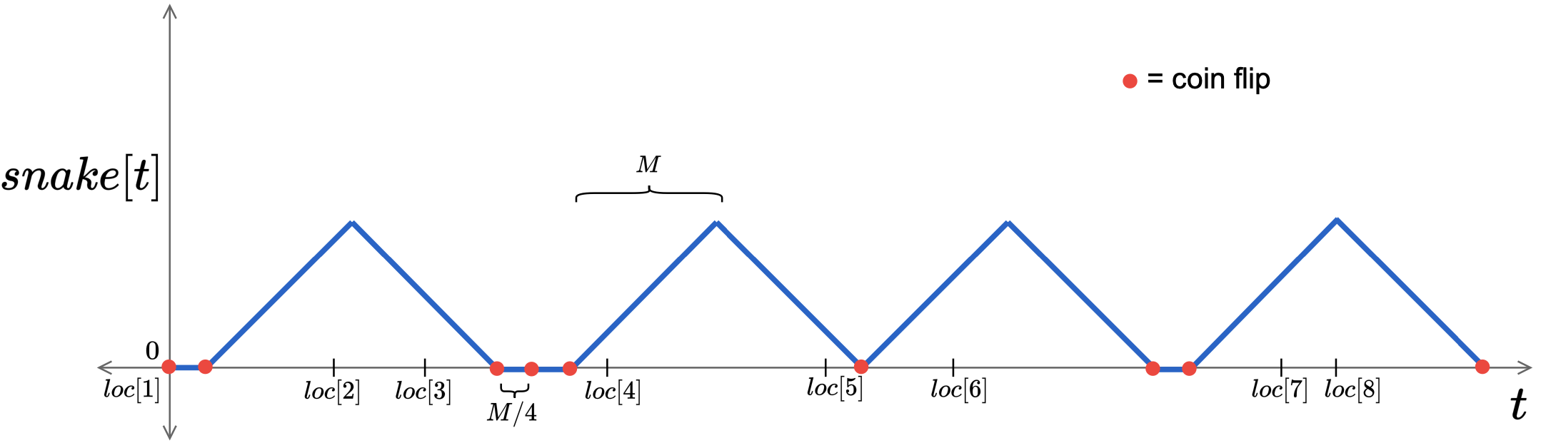
Figure 1: Lazy snaking with fixed cap.

We will require the following claim, which says that for every pair of nodes, lazy snaking does not overestimate their distance, and also covers at least a constant fraction of their distance in expectation.

Claim 4.4.

Let $embedding=\textsc{LazySnake}(loc,M)$. For every fixed pair of nodes $x_{i}$ and $x_{j}$,

$$\text{(1) }\operatorname{{Pr}}\left[|embedding[i]-embedding[j]|\leq d^{{M}}_{\mathrm{cap}}(x_{i},x_{j})\right]=1.$$

$$\text{(2) }\operatorname{{\mathds{E}}}\left[|embedding[i]-embedding[j]|\right]\geq\Omega(1)\cdot d^{{M}}_{\mathrm{cap}}(x_{i},x_{j}).$$

Proof.

The first part of the claim is straightforward, since snaking can only reduce distance between two nodes.
For the second part, let $i<j$ without loss of generality. Let $E_{1}$ be the event that $snake=0$ for some $t\in[\max(0,loc[i]-2M),loc[i]]$. Since the width that we snake over (if at all we are not at rest) is $M$, observe that $\operatorname{{Pr}}[E_{1}]=1$. We have three cases:
Case 1: $1\leq|loc[i]-loc[j]|\leq M.$
In this case, $d^{{M}}_{\mathrm{cap}}(x_{i},x_{j})=|loc[i]-loc[j]|$. Let $E_{2}$ be the event that $snake=0$ for some $t^{\prime}=[loc[i]-M/4,loc[i]]$. Then, $\operatorname{{Pr}}[E_{2}|E_{1}]\geq\left(\frac{1}{2}\right)^{8}=\Omega(1)$. This is because, the time to reach $loc[i]$ from $t$ is at most $2M$, and in this duration, we flip the “rest” coin at most $\frac{2M}{M/4}=8=O(1)$ times to arrive at such a $t^{\prime}$. Now, conditioned on $E_{2}$, we have that with probability $1/2$, we choose to move and snake for a width $M$, and if that happens, we have that that $0\leq embedding[i]\leq M/4$. Then, since $|loc[i]-loc[j]|\leq M$, we will have $embedding[j]-embedding[i]\geq\frac{1}{2}(loc[j]-loc[i])$. This is because, in the worst case, $embedding[i]=M/4$, and $loc[j]=loc[i]+M$, in which case $embedding[j]=3M/4$ after snaking around once. Since we only had to condition on a constant number of coin flips to obtain this,

$$\operatorname{{\mathds{E}}}\left[|embedding[i]-embedding[j]|\right] \geq\operatorname{{Pr}}[E_{1},E_{2}]\cdot\operatorname{{\mathds{E}}}\left[|embedding[i]-embedding[j]|~{}|~{}E_{1},E_{2}\right]$$

$$\geq\Omega(1)\cdot|loc[i]-loc[j]|.$$

Case 2: $M<|loc[i]-loc[j]|\leq 4M.$
In this case, $d^{{M}}_{\mathrm{cap}}(x_{i},x_{j})=M$. Let $E_{2}$ be the event that $embedding[i]=0$ and $snake=0$ for some $t^{\prime}\in[loc[j]-M,loc[j]-3M/4]$. Then, we have that $\operatorname{{Pr}}[E_{2}|E_{1}]\geq\Omega(1)$. This is because, to arrive at such a $t^{\prime}$ starting from $t$ while also ensuring that $embedding[i]=0$, we may flip at most $\frac{2M+3M}{M/4}=O(1)$ “rest” coins from time $t$ — this happens with probability at least $\Omega(1)$. Thereafter, conditioned on $E_{2}$, the coin flips “snake” with probability at least $1/2$, and this ensures that $embedding[j]\geq 3M/4$, which in turn gives $|embedding[i]-embedding[j]|\geq 3M/4$. Again, since we only had conditioned on $O(1)$, we get that

$$\operatorname{{\mathds{E}}}\left[|embedding[i]-embedding[j]|\right] \geq\operatorname{{Pr}}[E_{1},E_{2}]\cdot\operatorname{{\mathds{E}}}\left[|embedding[i]-embedding[j]|~{}|~{}E_{1},E_{2}\right]$$

$$\geq\Omega(1)\cdot M.$$

Case 3: $|loc[i]-loc[j]|>4M.$
Here as well, $d^{{M}}_{\mathrm{cap}}(x_{i},x_{j})=M$. First, just as in Case 1 above, let $E_{2}$ be the event that $snake=0$ for some $t^{\prime}=[loc[i]-M/4,loc[i]]$, for which we saw that $\operatorname{{Pr}}[E_{2}|E_{1}]\geq\Omega(1)$. Note that $E_{1},E_{2}$ together ensure that $embedding[i]\leq M/4$. Now, let $E_{3}$ be the event that $snake=0$ for some $t^{\prime\prime}\in[loc[j]-4M,loc[j]-2M]$. Since $|loc[i]-loc[j]|>4M$, there exists such a $t^{\prime\prime}>t^{\prime}$ with certainty, for which we have not yet assumed any conditioning, i.e., $\operatorname{{Pr}}[E_{3}|E_{2},E_{1}]=1$. Now, following $E_{3}$, with $\frac{3M}{M/4}=O(1)$ “rest” flips (happens with probability at least $\Omega(1)$), we ensure that $snake=0$ up until some $t^{\prime\prime\prime}\in[loc[j]-M,loc[j]-3M/4]$. Thereafter, we may flip a “snake”, ensuring that $embedding[j]\geq 3M/4$. Putting together, we get

$$\operatorname{{\mathds{E}}}\left[|embedding[i]-embedding[j]|\right] \geq\operatorname{{Pr}}[E_{1},E_{2},E_{3}]\cdot\operatorname{{\mathds{E}}}\left[|embedding[i]-embedding[j]|~{}|~{}E_{1},E_{2},E_{3}\right]$$

$$\geq\Omega(1)\cdot M.$$

∎

Using $O(\log n)$ dimensions, we can then boost the in-expectation guarantee of 4.4 to obtain the following theorem.

Theorem 4 (Fixed cap line into $\ell_{1}$).

$(L_{n},d^{{M}}_{\mathrm{cap}})$ can be embedded into $(\mathds{R}^{d},\ell_{1})$ where $d=O(\log n)$ with $\Theta(1)$ distortion.

Proof.

Let us invoke LazySnake$(loc,M)$ $N$ times to obtain $N$ independent copies $embedding_{1},\dots,embedding_{N}$ for all the nodes. Let $X^{(l)}_{ij}=|embedding_{l}[i]-embedding_{l}[j]|$. Then, observe that $0\leq X^{(l)}_{ij}\leq d^{{M}}_{\mathrm{cap}}(x_{i},x_{j})$. Furthermore, 4.4 gives that $\operatorname{{\mathds{E}}}\left[\sum_{k=1}^{N}X^{(l)}_{ij}\right]\geq cNd^{{M}}_{\mathrm{cap}}(x_{i},x_{j})$ for some constant $c>0$. Hoeffding’s inequality then gives us

$$\operatorname{{Pr}}\left[\sum_{l=1}^{N}X^{(l)}_{ij}\leq\frac{cNd^{{M}}_{\mathrm{cap}}(x_{i},x_{j})}{2}\right]\leq 2\exp\left(-\Theta(N)\right),$$

or rather, choosing $N=C\log n$ for an appropriately large constant $C$ gives

$$\operatorname{{Pr}}\left[\frac{1}{N}\sum_{l=1}^{N}X^{(l)}_{ij}\leq\frac{c}{2}\cdot d^{{M}}_{\mathrm{cap}}(x_{i},x_{j})\right]\leq\frac{2}{n^{3}}.$$

Furthermore, since the embedding never overestimates distances, observe that

$$\operatorname{{Pr}}\left[\frac{1}{N}\sum_{l=1}^{N}X^{(l)}_{ij}>d^{{M}}_{\mathrm{cap}}(x_{i},x_{j})\right]=0.$$

We can therefore rescale each $embedding_{k}$ as $embedding_{k}\leftarrow embedding_{k}/N$, and union bound over all the $<n^{2}$ pairs $i,j$ to obtain that

$$\operatorname{{Pr}}\left[\forall i,j:~{}\Omega(1)\cdot d^{{M}}_{\mathrm{cap}}(x_{i},x_{j})\leq\sum_{l=1}^{N}|embedding_{l}[i]-embedding_{l}[j]|\leq d^{{M}}_{\mathrm{cap}}(x_{i},x_{j})\right]>0,$$

which in particular, implies that there exists such an embedding that obtains $\Theta(1)$ distortion with $N=O(\log n)$ dimensions. ∎

4.2.2 Fixed Cap Tree Metrics

Consider now a tree $T_{n}$ on $n$ vertices $x_{1},\dots,x_{n}$, for which recall that the distance is given by $d(x_{i},x_{j})=\sum_{e\in x_{i}\to x_{j}}e$. Again, we consider the (fixed) cap version of the tree metric distance, given by

$$d^{{M}}_{\mathrm{cap}}(x_{i},x_{j})=\min(d(x_{i},x_{j}),M).$$ (10)

We will show that $(T_{n},d^{{M}}_{\mathrm{cap}})$ also embeds into $\ell_{1}$ using $O(\log^{2}n)$ dimensions and constant distortion.

First, let us obtain the caterpillar decomposition (stated in Section 3.5) of $T_{n}$. Let $C_{1},C_{2},\dots,C_{m}$ denote the caterpillars in its caterpillar decomposition, where each $C_{i}=\{e_{i_{1}},\dots,e_{i_{l}}\}$ is a simple path in the tree. The length of $C_{i}$ is the sum of the weights of the edges that it is made up of. We will first quickly see how the caterpillar decomposition yields an isometric embedding of the tree metric into $\ell_{1}$, while possibly using a lot many dimensions. We will have a coordinate in the embedding dedicated for every caterpillar in the decomposition -- thus, the number of dimensions can be as large as the number of edges in the tree, i.e., $\Omega(n)$. For every node $x_{i}$, we walk up from $x_{i}$ to the root, and for every caterpillar that we touch (at most $\log n$ of them), we record the length traversed on that caterpillar at the coordinate dedicated for it. Thus, we will end up with a $\log n$-sparse embedding for every node. We can see that this is an isometric embedding, because for any pair of nodes, the lengths on the caterpillars from their least common ancestor up to root get canceled out when we take the difference of their embeddings, and only the lengths on caterpillars on the path joining them survive.

Now, we describe a slight modification to the above embedding, which possibly increases the dimensions even more, but still ensures that the embedding is isometric, and will be useful for constructing our final low-dimensional embedding for the capped tree metric with cap $M$. For any caterpillar $C_{i}$ whose length is at most $M$, we do nothing. For caterpillars having length larger than $M$, we split it up into snippets of size exactly $M/\log n$, and possibly one left-over snippet of size smaller than $M/\log n$. Having snipped each caterpillar like so, let $S_{1},\dots,S_{s}$ be all the resulting snippets --- we will dedicate a single coordinate in the embedding to each $S_{i}$. As before, for every node, we walk up from the node to the root, and record the length of each snippet we traverse at the corresponding coordinate. Let this embedding be denoted by $\mathrm{SC}$ (short for Snipped Caterpillar) i.e., $\mathrm{SC}(x_{i})$ is a vector of size $s$ for each node $x_{i}$. This embedding is still isometric, however, the number of snippets $s$ can now be huge, if a large number of the caterpillars had length $\gg M$.

We will now make a couple observations on the structure of the vector $\mathrm{SC}(x_{i})-\mathrm{SC}(x_{j})$ for any pair of nodes $x_{i}$ and $x_{j}$.

Claim 4.5.

If $d(x_{i},x_{j})\leq M$, then $\mathrm{SC}(x_{i})-\mathrm{SC}(x_{j})$ has at most $6\log n$ non-zero coordinates, and each of these coordinates is at most $M/\log n$ in magnitude.

Proof.

Let $z=\mathrm{SC}(x_{i})-\mathrm{SC}(x_{j})$. The only non-zero coordinates in $z$ correspond to the caterpillar snippets on the path joining $x_{i}$ and $x_{j}$. First, let us count the number of full $M/\log n$ sized snippets on this path — since $\|z\|_{1}=d(x_{i},x_{j})\leq M$, we can have at most $\log n$ many such snippets. Now, let us count the number of non-zero coordinates contributed by snippets of length $<M/\log n$. These could either be due to caterpillars that were smaller than $M/\log n$, and never got snipped — there could be at most $2\log n$ many of these, since the (unsnipped) caterpillar embeddings of both $x_{i}$ and $x_{j}$ are $\log n$ sparse. Or, these could be due to partial snippets on the path joining $x_{i}$ and $x_{j}$. Observe that we can have at most one partial snippet per whole caterpillar on this path (except possibly an extra at the least common ancestor), and thus, we can again only have $2\log n+1\leq 3\log n$ many of these in total. Together, we get $\log n+2\log n+3\log n=6\log n$ many non-zero coordinates, as claimed. Finally, by construction, each coordinate in both $\mathrm{SC}(x_{i})$ and $\mathrm{SC}(x_{j})$ is at most $M/\log n$, and hence the difference can be at most $M/\log n$ in magnitude. ∎

Claim 4.6.

If $d(x_{i},x_{j})>M$, then $\mathrm{SC}(x_{i})-\mathrm{SC}(x_{j})$ contains a set of $\frac{3}{4}\log n$ non-zero coordinates, each of which is at least $\frac{M}{20\log n}$ and at most $\frac{M}{\log n}$ in magnitude, and the sum of these coordinates is at least $3M/4$.

Proof.

Again, let $z=\mathrm{SC}(x_{i})-\mathrm{SC}(x_{j})$. First, let us count the number of snippets on the path joining $x_{i}$ and $x_{j}$ that are less than $\frac{M}{20\log n}$ in absolute value. Either these arise due to unsnipped-caterpillars of length smaller than $M/\log n$ in the embeddings of $x_{i}$ and $x_{j}$ — there can be at most $2\log n$ many of these; or these arise due to partial snippets on the path joining them — there are again at most $2\log n+1\leq 3\log n$ many of these, as argued above. Thus, there can only be at most $5\log n$ many coordinates having magnitude smaller than $\frac{M}{20\log n}$ in $z$. These coordinates account for length at most $M/4$ out of $\|z\|_{1}$. All the other coordinates necessarily have magnitude at least $\frac{M}{20\log n}$, but also at most $M/\log n$ by construction. Since $\|z\|=d(x_{i},x_{j})>M$, these other coordinates have to account for at least $3M/4$ of the length. Thus, there needs to be a set of at least $\frac{3M}{4}\cdot\frac{\log n}{M}=\frac{3}{4}\log n$ many coordinates, each of which is at least $\frac{M}{20\log n}$, and whose sum is at least $3M/4$ as required. ∎

Now, for $k=6\log n$, consider choosing a uniformly random hash function $h:[s]\to[k]$, where recall that $s$ is the total number of caterpillar snippets. For each node $x_{i}$, let $\mathrm{HSC}(x_{i})$ (short for Hashed Snipped Caterpillar) be a vector of size $6\log n$, defined in the following. This will be the building block of our final $O(\log^{2}n)$ sized embedding.

$$\mathrm{HSC}(x_{i})[p]=\sum_{q\in[s]:h(q)=p}\mathrm{SC}(x_{i})[q]\qquad\text{for }p\in\{1,\dots,k\}.$$ (11)

Now, we interpret each coordinate of $\mathrm{HSC}$ as defining a line metric, over which we will do lazy snaking. Concretely, for each $p\in[k]$, let $loc_{p}[i]=\mathrm{HSC}(x_{i})[p]$ --- note that for the root $x_{1}$, $loc_{p}[1]=0$ for all $p$, since $\mathrm{SC}(x_{i})=0^{s}$. Let $sloc_{p}=\textsc{LazySnake}(loc_{p},M/\log n)$, and consider the representation of each node $x_{i}$ as

$$embedding[i]=(sloc_{1}[i],sloc_{2}[i],\dots,sloc_{k}[i]).$$ (12)

First, we make the following simple claim:

Claim 4.7 (No overestimation).

Fix any pair of nodes $x_{i}$ and $x_{j}$. Then, with probability 1,

$$\|embedding[i]-embedding[j]\|_{1}\leq 6d^{{M}}_{\mathrm{cap}}(x_{i},x_{j}).$$

Proof.

We have two cases:
Case 1: $d(x_{i},x_{j})\leq M.$
In this case, $d^{{M}}_{\mathrm{cap}}(x_{i},x_{j})=d(x_{i},x_{j})$. Observe that

$$\|embedding[i]-embedding[j]\|_{1} =\sum_{p=1}^{k}\left|sloc_{p}[i]-sloc_{p}[j]\right|$$

$$\leq\sum_{p=1}^{k}\left|loc_{p}[i]-loc_{p}[j]\right|\quad\text{(snaking never overestimates distances)}$$

$$=\sum_{p=1}^{k}\left|\sum_{q\in[s]:h(q)=p}(\mathrm{SC}(x_{i})[q]-\mathrm{SC}(x_{j})[q])\right|$$

$$\leq\sum_{p=1}^{k}\sum_{q\in[s]:h(q)=p}\left|\mathrm{SC}(x_{i})[q]-\mathrm{SC}(x_{j})[q]\right|$$

$$=d(x_{i},x_{j}).$$

Case 2: $d(x_{i},x_{j})>M.$
In this case, $d^{{M}}_{\mathrm{cap}}(x_{i},x_{j})=M$. We have

$$\|embedding[i]-embedding[j]\|_{1} =\sum_{p=1}^{k}\left|sloc_{p}[i]-sloc_{p}[j]\right|$$

$$\leq\sum_{p=1}^{k}\frac{M}{\log n}\qquad\left(\text{snaking width is }\frac{M}{\log n}\right)$$

$$\leq 6M.$$

∎

4.7 ensures that the embedding never overestimates distances beyond a constant factor. However, we also have the following nice property, which ensures that in expectation, the embedding captures at least a constant fraction of the distance between any fixed pair of nodes.

Lemma 4.8 (No underestimation).

Fix any pair of nodes $x_{i}$ and $x_{j}$, and fix $p\in[k]$. Then, we have that

$$\operatorname{{\mathds{E}}}\left[\left|sloc_{p}[i]-sloc_{p}[j]\right|\right] =\operatorname{{\mathds{E}}}_{h}\operatorname{{\mathds{E}}}_{\mathrm{snake}}\left[\left|sloc_{p}[i]-sloc_{p}[j]\right|\right]\geq\frac{\Omega(1)}{k}\cdot d^{{M}}_{\mathrm{cap}}(x_{i},x_{j}).$$

Thus, by linearity of expectation,

$$\operatorname{{\mathds{E}}}\left[\|embedding[i]-embedding[j]\|_{1}\right]=\operatorname{{\mathds{E}}}\left[\sum_{p=1}^{k}\left|sloc_{p}[i]-sloc_{p}[j]\right|\right]\geq\Omega(1)\cdot d^{{M}}_{\mathrm{cap}}(x_{i},x_{j}).$$

Proof.

We have two cases:
Case 1: $d(x_{i},x_{j})\leq M.$
In this case, $d^{{M}}_{\mathrm{cap}}(x_{i},x_{j})=d(x_{i},x_{j})$. Recall from 4.5 that $\mathrm{SC}(x_{i})-\mathrm{SC}(x_{j})$ has at most $6\log n$ non-zero coordinates and each of these coordinates is at most $\frac{M}{\log n}$ in magnitude. Let us possibly include some zero coordinates, so that we have exactly $k=6\log n$ of these “special” coordinates $c_{1},\dots,c_{r},\dots,c_{k}$. Observe that $\sum_{r=1}^{k}|\mathrm{SC}(x_{i})[c_{r}]-\mathrm{SC}(x_{j})[c_{r}]|=d(x_{i},x_{j})$, because the snipped-caterpillar embedding is isometric. Let us condition on the realization of the hash function $h$, which is independent of the randomness in the snaking. Conditioned on this realization, for $loc_{p}[i]=\mathrm{HSC}(x_{i})[p]$ and $sloc_{p}=\textsc{LazySnake}(loc_{p},M/\log n)$ we have from 4.4 that

$$\operatorname{{\mathds{E}}}_{\mathrm{snake}}\left[|sloc_{p}[i]-sloc_{p}[j]|\right]\geq\Omega(1)\cdot d^{{M/\log n}}_{\mathrm{cap}}(loc_{p}[i],loc_{p}[j]).$$

Now, taking an expectation with respect to the choice of the hash function, we get

$$\operatorname{{\mathds{E}}}_{h}\operatorname{{\mathds{E}}}_{\mathrm{snake}}\left[|sloc_{p}[i]-sloc_{p}[j]|\right]\geq\Omega(1)\cdot\operatorname{{\mathds{E}}}_{h}\left[d^{{M/\log n}}_{\mathrm{cap}}(loc_{p}[i],loc_{p}[j])\right].$$

Let $A$ be the event that only one of the $k$ special coordinates hashes to $p$. Then, we have that $\operatorname{{Pr}}[A]=\left(1-\frac{1}{k}\right)^{k-1}\geq\frac{1}{e}=\Omega(1)$, yielding

$$\operatorname{{\mathds{E}}}_{h}\left[d^{{M/\log n}}_{\mathrm{cap}}(loc_{p}[i],loc_{p}[j])\right] \geq\Omega(1)\cdot\operatorname{{\mathds{E}}}_{h}\left[d^{{M/\log n}}_{\mathrm{cap}}(loc_{p}[i],loc_{p}[j])~{}|~{}A\right]$$

Furthermore, conditioned on $A$, we have

$$\operatorname{{\mathds{E}}}_{h}\left[d^{{M/\log n}}_{\mathrm{cap}}(loc_{p}[i],loc_{p}[j])~{}|~{}A\right]$$

$$\qquad=\sum_{r=1}^{k}\frac{1}{k}\cdot\operatorname{{\mathds{E}}}_{h}\left[d^{{M/\log n}}_{\mathrm{cap}}(loc_{p}[i],loc_{p}[j])~{}|~{}\text{only $r^{\text{th}}$ special coordinate hashes to $p$}\right].$$

But now, observe that if only the $r^{\text{th}}$ special coordinate hashes to $p$, we have $d^{{M/\log n}}_{\mathrm{cap}}(loc_{p}[i],loc_{p}[j])=|\mathrm{SC}(x_{i})[c_{r}]-\mathrm{SC}(x_{j})[c_{r}]|$. This is because $|\mathrm{SC}(x_{i})[c_{r}]-\mathrm{SC}(x_{j})[c_{r}]|$ is at most $M/\log n$, which is smaller than the cap. Finally, recalling that $\sum_{r=1}^{k}|\mathrm{SC}(x_{i})[c_{r}]-\mathrm{SC}(x_{j})[c_{r}]|=d(x_{i},x_{j})$, we get

$$\operatorname{{\mathds{E}}}_{h}\left[d^{{M/\log n}}_{\mathrm{cap}}(loc_{p}[i],loc_{p}[j])~{}|~{}A\right] =\sum_{r=1}^{k}\frac{1}{k}\left|\mathrm{SC}(x_{i})[c_{r}]-\mathrm{SC}(x_{j})[c_{r}]\right|=\frac{1}{k}\cdot d(x_{i},x_{j}).$$

Putting everything together, we get

$$\operatorname{{\mathds{E}}}_{h}\operatorname{{\mathds{E}}}_{\mathrm{snake}}\left[|sloc_{p}[i]-sloc_{p}[j]|\right] \geq\frac{\Omega(1)}{k}\cdot d(x_{i},x_{j})=\Omega(1)\cdot\frac{d^{{M}}_{\mathrm{cap}}(x_{i},x_{j})}{k}.$$

Case 2: $d(x_{i},x_{j})>M.$
In this case, $d^{{M}}_{\mathrm{cap}}(x_{i},x_{j})=M$. Recall from 4.6 that $\mathrm{SC}(x_{i})-\mathrm{SC}(x_{j})$ has a set of $k^{\prime}=\frac{3}{4}\log n$ non-zero “special” coordinates $c_{1},\dots,c_{r},\dots,c_{k^{\prime}}$, each of which is at least $\frac{M}{20\log n}$ and at most $\frac{M}{\log n}$ in magnitude. Let $A$ be the event that the non-special coordinates that get hashed to $p$ amount for a distance of at least $\frac{M}{100\log n}$. Concretely, under $A$, $\left|\sum_{q\in[s]:q\text{ not special},h(q)=p}(SC(x_{i})[q]-SC(x_{j})[q])\right|\geq\frac{M}{100\log n}$. We have that

$$\operatorname{{\mathds{E}}}\left[|sloc_{p}[i]-sloc_{p}[j]|\right] =\operatorname{{Pr}}[A]\cdot\operatorname{{\mathds{E}}}\left[|sloc_{p}[i]-sloc_{p}[j]|~{}|~{}A\right]$$

$$\quad+\operatorname{{Pr}}[\neg A]\cdot\operatorname{{\mathds{E}}}\left[|sloc_{p}[i]-sloc_{p}[j]|~{}|~{}\neg A\right]$$

Conditioned on $A$, we are happy if none of the special coordinates hash to $p$, which happens with probability $\left(1-\frac{1}{k}\right)^{k^{\prime}}\geq\exp\left(-\frac{k^{\prime}}{\sqrt{k(k-1)}}\right)=\exp\left(-\frac{1}{8}\sqrt{\frac{6\log n}{6\log n-1}}\right)\geq 1/e=\Omega(1)$ for $n\geq 2$. In this case, lazy snaking will capture at least a constant fraction of $\frac{M}{100\log n}$, yielding

$$\operatorname{{\mathds{E}}}\left[|sloc_{p}[i]-sloc_{p}[j]|~{}|~{}A\right] \geq\Omega(1)\cdot\frac{M}{100\log n}.$$

If $A$ does not occur, we have that $\left|\sum_{q\in[s]:q\text{ not special},h(q)=p}(SC(x_{i})[q]-SC(x_{j})[q])\right|<\frac{M}{100\log n}$. In this case, we are happy if exactly one of the special coordinates hashes to $p$, which happens with probability $\left(1-\frac{1}{k}\right)^{k^{\prime}-1}\geq\left(1-\frac{1}{k}\right)^{k^{\prime}}\geq 1/e=\Omega(1)$. This will ensure a distance of at least $\frac{M}{20\log n}-\frac{M}{100\log n}=\frac{M}{25\log n}$, of which lazy snaking will capture at least a constant fraction in expectation, yielding

$$\operatorname{{\mathds{E}}}\left[|sloc_{p}[i]-sloc_{p}[j]|~{}|~{}\neg A\right] \geq\Omega(1)\cdot\frac{M}{25\log n}.$$

In total, we get that

$$\operatorname{{\mathds{E}}}\left[|sloc_{p}[i]-sloc_{p}[j]|\right] \geq\operatorname{{Pr}}[A]\cdot\Omega(1)\cdot\frac{M}{100\log n}+\operatorname{{Pr}}[\neg A]\cdot\Omega(1)\cdot\frac{M}{25\log n}$$

$$\geq\Omega(1)\cdot\frac{M}{100\log n}\left(\operatorname{{Pr}}[A]+\operatorname{{Pr}}[\neg A]\right)$$

$$=\Omega(1)\cdot\frac{M}{100\log n}=\Omega(1)\cdot\frac{M}{k}=\Omega(1)\cdot\frac{d^{{M}}_{\mathrm{cap}}(x_{i},x_{j})}{k}.$$

∎

As in the case of the capped line metric, using $O(\log n)$ independent repetitions of the above, we obtain the following theorem.

Theorem 5 (Fixed cap tree into $\ell_{1}$).

$(T_{n},d^{{M}}_{\mathrm{cap}})$ can be embedded into $(\mathds{R}^{d},\ell_{1})$ where $d=O(\log^{2}n)$ with $\Theta(1)$ distortion.

Proof.

Let us obtain $N$ independent copies $embedding_{1},\dots,embedding_{N}$ of the embedding in Equation 12. Note that each of these is an embedding of size $6\log n$. Let $X^{(l)}_{ij}=\|embedding_{l}[i]-embedding_{l}[j]\|_{1}$. Then, observe that from 4.7, $0\leq X^{(l)}_{ij}\leq 6d^{{M}}_{\mathrm{cap}}(x_{i},x_{j})$. Furthermore, Lemma 4.8 gives that $\operatorname{{\mathds{E}}}\left[\sum_{l=1}^{N}X^{(l)}_{ij}\right]\geq cNd^{{M}}_{\mathrm{cap}}(x_{i},x_{j})$ for some absolute constant $c>0$. Hoeffding’s inequality then gives us

$$\operatorname{{Pr}}\left[\sum_{l=1}^{N}X^{(l)}_{ij}\leq\frac{cNd^{{M}}_{\mathrm{cap}}(x_{i},x_{j})}{2}\right]\leq 2\exp\left(-\Theta(N)\right),$$

or rather, choosing $N=C\log n$ for an appropriately large constant $C$ gives

$$\operatorname{{Pr}}\left[\frac{1}{N}\sum_{l=1}^{N}X^{(l)}_{ij}\leq\frac{c}{2}\cdot d^{{M}}_{\mathrm{cap}}(x_{i},x_{j})\right]\leq\frac{2}{n^{3}}.$$

Furthermore, since the embedding never overestimates distances (4.7), observe that

$$\operatorname{{Pr}}\left[\frac{1}{N}\sum_{l=1}^{N}X^{(l)}_{ij}>6d^{{M}}_{\mathrm{cap}}(x_{i},x_{j})\right]=0.$$

We can therefore rescale each coordinate in $embedding_{k}$ as $embedding_{k}\leftarrow embedding_{k}/N$, and union bound over all the $<n^{2}$ pairs $i,j$ to obtain that

$$\operatorname{{Pr}}\left[\forall i,j:~{}\Omega(1)\cdot d^{{M}}_{\mathrm{cap}}(x_{i},x_{j})\leq\sum_{l=1}^{N}\|embedding_{l}[i]-embedding_{l}[j]\|_{1}\leq O(1)\cdot d^{{M}}_{\mathrm{cap}}(x_{i},x_{j})\right]>0,$$

which in particular, implies that there exists such an embedding that obtains $\Theta(1)$ distortion with $N=O(\log^{2}n)$ dimensions. ∎

5 General Tree Ising Models

We now turn our attention to the more general and challenging case of tree Ising models on $n$ random variables $X_{1},\dots,X_{n}$ where each variable can additionally have a nonzero external field (Equation 2). Recall that these tree Ising models can be uniquely described by specifying marginal probabilities for every $X_{i}$, and joint probabilities for every pair $(X_{i},X_{j})$ that corresponds to an edge in the tree.

To exhaustively capture the probability of disagreement between two variables $X_{i}$ and $X_{j}$, we end up requiring to crucially capture contribution towards this by the ‘‘independence" between the variables. In the typical notion of independence, this could be thought of in terms of being distance that grows with $H(X_{i}|X_{j})$ or $H(X_{j}|X_{i})$, where $H$ is the standard Shannon entropy. However, conditional Shannon entropy $H(X_{i}|X_{j})$ seems at first glance an unwieldy quantity from the perspective of embedding into $\ell_{1}$ (for reasons like, e.g., the behavior of $H(X_{i})$ as $X_{i}\rightarrow 0$). We define an alternative seemingly simpler quantity, which we call ‘‘Bernoulli Randomness", that essentially captures what we are hoping for.

5.1 Bernoulli Randomness

Definition 1 (Bernoulli Randomness).

Any binary random variable $X$ can be written as the mixture of an unbiased random variable and a deterministic (i.e. single state of support) variable. Let $\operatorname{{Br}}(X)$ be the weight of the mixture on the unbiased variable. We can see that $\operatorname{{Br}}(X)=2\cdot\min(\operatorname{{Pr}}[X=0],\operatorname{{Pr}}[X=1])$.

A philosophical interpretation of Bernoulli randomness is that it corresponds to the probability that $X$ is determined by a purely random coin flip, instead of being deterministically chosen. Like Shannon entropy, Bernoulli randomness increases as $X$ becomes less biased.

We similarly define conditional Bernoulli randomness:

Definition 2 (Conditional Bernoulli Randomness).

$\operatorname{{Br}}(X|Y)=\sum_{y\in\{0,1\}}\operatorname{{Pr}}(Y=y)\cdot\operatorname{{Br}}(X|Y=y)=\sum_{y}2\cdot\min(\operatorname{{Pr}}(X=0,Y=y),\operatorname{{Pr}}(X=1,Y=y))$

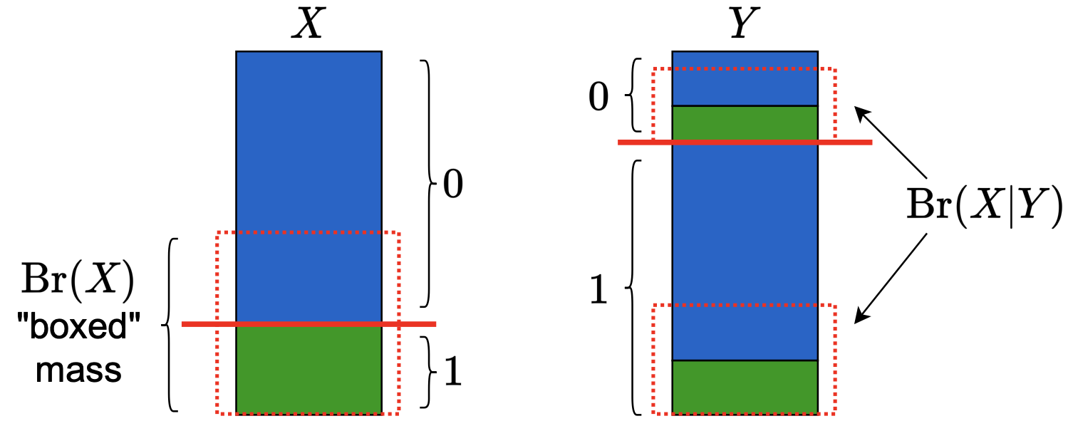
Figure 2: Bernoulli randomness and conditional Bernoulli randomness as ‘‘boxed’’ mass.

It helps a lot to keep Figure 2 in mind when thinking of Bernoulli randomness. The probability mass of $X$ has been divided by the red solid line into blue and green states corresponding to $\operatorname{{Pr}}[X=0]$ and $\operatorname{{Pr}}[X=1]$ respectively. Here, $\operatorname{{Br}}(X)$ is exactly the mass ‘‘boxed’’ by the red dashed line---there is an equal amount of green and blue mass in the box. Similarly, on the right, the blue and green mass of $X$ has been distributed in the states of $Y=0$ and $Y=1$ according to the joint distribution of $X$ and $Y$. The total boxed mass across both the states is precisely $\operatorname{{Br}}(X|Y)$.

We can lower bound the probability of disagreement between $X$ and $Y$ in terms of conditional Bernoulli randomness in a straightforward manner:

Lemma 5.1 ($\operatorname{{Br}}$ lower-bounds distance).

$\operatorname{{Pr}}[X\neq Y]\geq\frac{1}{2}\cdot\operatorname{{Br}}(Y|X),\frac{1}{2}\cdot\operatorname{{Br}}(X|Y)$.

Proof.

This is true because, for example, because if $Y$ is chosen via an unbiased coin from $X$ with probability $\operatorname{{Br}}(Y|X)$, then for each unbiased coin flip there is at least $1/2$ chance $X\neq Y$ and thus $\operatorname{{Pr}}[X\neq Y]\geq\frac{1}{2}\cdot\operatorname{{Br}}(Y|X)$. More formally,

$$\operatorname{{Pr}}[X\neq Y] =\operatorname{{Pr}}[X=0,Y=1]+\operatorname{{Pr}}[X=1,Y=0]$$

$$\geq\min(\operatorname{{Pr}}[X=0,Y=0],\operatorname{{Pr}}[X=0,Y=1])+\min(\operatorname{{Pr}}[X=1,Y=0],\operatorname{{Pr}}[X=1,Y=0])$$

$$=\frac{1}{2}\cdot\operatorname{{Br}}(Y|X).$$

The argument for $\operatorname{{Br}}(X|Y)$ is identical. ∎

The following result also nicely matches the intuition from Shannon entropy:

Claim 5.2 ($\operatorname{{Br}}$ maximized at independence).

Given two variables with fixed marginals $X,Y$, when optimizing over their joints it holds that $\operatorname{{Br}}(X|Y)$ and $\operatorname{{Br}}(Y|X)$ are both maximized when $X,Y$ are independent.

Proof.

We state the proof for $\operatorname{{Br}}(X|Y)$—the proof for $\operatorname{{Br}}(Y|X)$ is identical.

$$\operatorname{{Br}}(X|Y) =2(\min(\operatorname{{Pr}}[X=0,Y=0],\operatorname{{Pr}}[X=1,Y=0])+\min(\operatorname{{Pr}}[X=0,Y=1],\operatorname{{Pr}}[X=1,Y=1]))$$

$$\leq 2(\operatorname{{Pr}}[X=0,Y=0]+\operatorname{{Pr}}[X=0,Y=1])=2\operatorname{{Pr}}[X=0],$$

and similarly,

$$\operatorname{{Br}}(X|Y) =2(\min(\operatorname{{Pr}}[X=0,Y=0],\operatorname{{Pr}}[X=1,Y=0])+\min(\operatorname{{Pr}}[X=0,Y=1],\operatorname{{Pr}}[X=1,Y=1]))$$

$$\leq 2(\operatorname{{Pr}}[X=1,Y=0]+\operatorname{{Pr}}[X=1,Y=1])=2\operatorname{{Pr}}[X=1].$$

This means $\operatorname{{Br}}(X|Y)\leq 2\min(\operatorname{{Pr}}[X=0],\operatorname{{Pr}}[X=1])=\operatorname{{Br}}(X)$. Note that equality is attained when $X$ and $Y$ are independent. ∎

The niceness of the aforementioned claim is that the same statement is classically known to hold when $\operatorname{{Br}}$ terms are replaced with $H$ (Shannon entropy) terms. A key difference, however, is that while the independent joint distribution is the unique maximizer for Shannon entropy, there are often many maximizers for Bernoulli randomness. For example, consider random variables $X,Y$ with $p_{00}=0.1,p_{01}=0.2,p_{10}=0.2,p_{11}=0.5$. Here, $\operatorname{{Br}}(X|Y)=\operatorname{{Br}}(Y|X)=\operatorname{{Br}}(X)=\operatorname{{Br}}(Y)=0.6$, but $X$ and $Y$ are not independent. This indicates that although the notions share similar intuitions, there are key differences.

In our proof for tree Ising models, we will be studying the accumulation of conditional Bernoulli randomness. A simple lemma that may help see the niceness of this property (analogous to the data processing inequality for mutual information) is as follows:

Lemma 5.3 (Data Processing Inequality).

Consider a Bayesian network on a line specified by $X_{1}\to\dots\to X_{n}$. For any $i<j<k$, it must hold that $\operatorname{{Br}}(X_{i}|X_{k})\geq\operatorname{{Br}}(X_{i}|X_{j})$.

Proof.

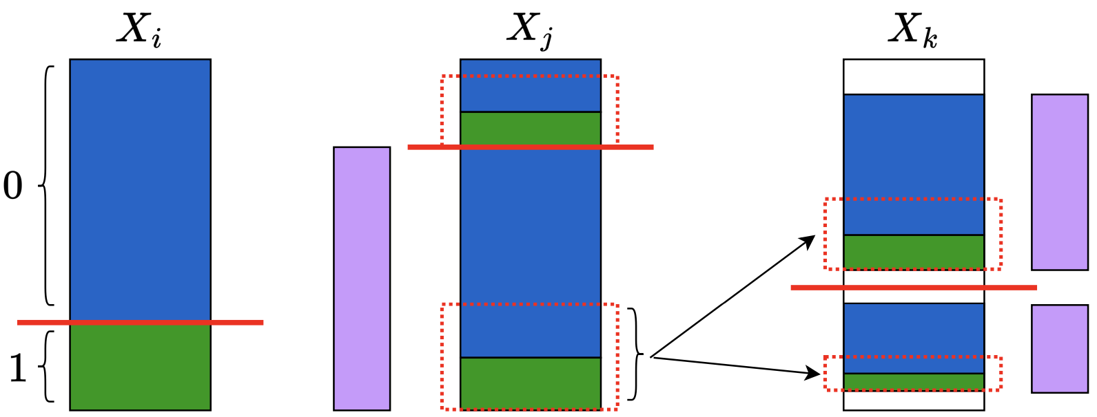
Figure 3: The ratio of blue and green mass within $X_{j}=0$ and $X_{j}=1$ is preserved when it gets distributed between $X_{k}=0$ and $X_{k}=1$. The picture above only shows this for the (purple) mass in state $X_{j}=1$. However, it is also true for the mass within state $X_{j}=0$ that would occupy the leftover white regions in $X_{k}$.

The proof is aided by the pictoral definition of conditional Bernoulli randomness in terms of “boxed” mass that we stated above. In Figure 3, blue mass corresponds to $X_{i}=0$ and green mass corresponds to $X_{i}=1$. The total boxed mass in $X_{j}$ corresponds to $\operatorname{{Br}}(X_{i}|X_{j})$. Observe that because of the Markov property, $\operatorname{{Pr}}[X_{i}|X_{j},X_{k}]=\operatorname{{Pr}}[X_{i}|X_{j}]$. Namely, the mass in the bucket $X_{j}=1$ must get distributed between the buckets $X_{k}=0$ and $X_{k}=1$ in a such a way that the blue-to-green ratio in both these buckets is equal to the ratio in $X_{j}=1$. Put another way, some fraction of the total mass in $X_{j}=1$ goes to the bucket $X_{k}=0$ and the remaining fraction goes to the bucket $X_{k}=1$. The same also happens to the mass in $X_{j}=0$. But observe that this preserves all the boxing of mass in $X_{j}$. Namely, all the boxed mass in $X_{j}$ remains boxed in $X_{k}$, and we can only gain additional boxed mass because of redistribution. Thus, the boxed mass in $X_{k}$ is at least as much as the boxed mass in $X_{j}$, which means that $\operatorname{{Br}}(X_{i}|X_{k})\geq\operatorname{{Br}}(X_{i}|X_{j})$. ∎

5.2 General Tree Ising Models Reduce to Lipschitz Cap Tree Metrics

In this section, we will transform the task of embedding general tree Ising models into $\ell_{1}$ to the task of embedding Lipschitz cap tree metrics into $\ell_{1}$. In what follows, we will reason about $\operatorname{{Pr}}[X_{i}\neq X_{j}]$ for nodes $X_{i}$ and $X_{j}$ in the tree Ising model. For this, we will imagine the tree to be rooted at $X_{i}$, with all edges pointing away from the root. This ensures that all the edges on the path from $X_{i}$ to $X_{j}$ are in the same direction, which will allow us to use convenient independence properties to reason about the evolution of conditional Bernoulli randomness as we traverse the path. Furthermore, this rooting assumption is without loss of generality, by the equivalence of tree Ising models and tree-structured Bayesian networks, as mentioned in Section 3.2.

For a node $X_{i}$ in the tree Ising model, let us define its bias $b(i)=\min(\operatorname{{Pr}}[X_{i}=0],\operatorname{{Pr}}[X_{i}=1])$. The following inequality upper-bounds the absolute difference in the biases of $X_{i}$ and $X_{j}$ in terms of Bernoulli randomness and the probability that they disagree.

Lemma 5.4.

Let $b(i)=\min(\operatorname{{Pr}}[X_{i}=0],\operatorname{{Pr}}[X_{i}=1])$.

1. $b(i)-b(j)\leq\frac{1}{2}\cdot\operatorname{{Br}}(X_{i}|X_{j}).$

2. $|b(i)-b(j)|\leq\operatorname{{Pr}}[X_{i}\neq X_{j}].$

Proof.

Suppose $\operatorname{{Pr}}[X_{i}=0],\operatorname{{Pr}}[X_{j}=0]\geq\frac{1}{2}$ without loss of generality. Then,

$$\operatorname{{Br}}(X_{i}|X_{j}) \geq 2\cdot\min_{x}\operatorname{{Pr}}[X_{i}=x,X_{j}=0]=2\cdot\left(\operatorname{{Pr}}[X_{j}=0]-\max_{x}\operatorname{{Pr}}[X_{i}=x,X_{j}=0]\right)$$

$$\geq 2\cdot\left(\operatorname{{Pr}}[X_{j}=0]-\max_{x}\operatorname{{Pr}}[X_{i}=x]\right)=2\cdot\left((1-b(j))-(1-b(i))\right)=2\cdot\left(b(i)-b(j)\right)$$

Repeating the calculation above with $\operatorname{{Br}}(X_{j}|X_{i})$ yields $\operatorname{{Br}}(X_{j}|X_{i})\geq 2\cdot\left(b(j)-b(i)\right)$. Thus, we get

$$|b(i)-b(j)|\leq\frac{1}{2}\cdot\max\left(\operatorname{{Br}}(X_{i},X_{j}),\operatorname{{Br}}(X_{j}|X_{i})\right)\leq\operatorname{{Pr}}[X_{i}\neq X_{j}]$$

where we used Lemma 5.1 in the last step. ∎

Now, let us define a strange but necessary quantity, that captures a ‘‘surprise" event when we traverse an edge.

Definition 3 (Cross).

We define an edge $e=(X_{u},X_{v})$ as being a “cross” if $\operatorname{{Pr}}[X_{u}=0,X_{v}=1]+\operatorname{{Pr}}[X_{u}=1,X_{v}=0]>\operatorname{{Pr}}[X_{u}=0,X_{v}=0]+\operatorname{{Pr}}[X_{u}=1,X_{v}=1]$, or equivalently $\operatorname{{Pr}}[X_{u}=0,X_{v}=1]+\operatorname{{Pr}}[X_{u}=1,X_{v}=0]>\frac{1}{2}$.

We will show how distance can be related to three sources and how we can embed these sources well.

Lemma 5.5.

Each of the following quantities is upper bounded by $O(\operatorname{{Pr}}[X_{i}\neq X_{j}])$:

1. Difference in marginals: $d_{\mathrm{marg}}(i,j)=|\operatorname{{Pr}}[X_{i}=0]-\operatorname{{Pr}}[X_{j}=0]|$.

2. Bernoulli randomness: $d_{\operatorname{{Br}}}(i,j)=\operatorname{{Br}}(X_{i}|X_{j})$.

3. Negative correlation: $d_{\mathrm{negcor}}(i,j)=\begin{cases}\max(b(i),b(j))&\text{if number of crosses between $i$ and $j$ is odd.}\\ |b(i)-b(j)|&\text{if number of crosses between $i$ and $j$ is even.}\end{cases}$

Proof.

For part (a), observe that

$$|\operatorname{{Pr}}[X_{i}=0]-\operatorname{{Pr}}[X_{j}=0]| =|\operatorname{{Pr}}[X_{i}=0,X_{j}=1]-\operatorname{{Pr}}[X_{i}=1,X_{j}=0]$$

$$\leq\operatorname{{Pr}}[X_{i}=0,X_{j}=1]+\operatorname{{Pr}}[X_{i}=1,X_{j}=0]=\operatorname{{Pr}}[X_{i}\neq X_{j}].$$

Part (b) follows from Lemma 5.1 above. Part (c) is relatively most involved. Note that the “even crosses” case follows from Lemma 5.4. For the “odd crosses” case, we have

Claim 5.6.

If there are an odd number of crosses between $X_{i}$ and $X_{j}$, then $\min(b(i),b(j))=O(\operatorname{{Pr}}[X_{i}\neq X_{j}])$.

Proof.

Case 1: $\operatorname{{Br}}(X_{i}|X_{j})=2\cdot b(i)$. In this case, we use (2) to get

$$\min(b(i),b(j))\leq b(i)=\frac{1}{2}\operatorname{{Br}}(X_{i}|X_{j})=O(\operatorname{{Pr}}[X_{i}\neq X_{j}]).$$

Case 2: $\operatorname{{Br}}(X_{i}|X_{j})\geq\frac{1}{2}$. In this case, again by (2) we know

$$\min(b(i),b(j))\leq\frac{1}{2}\leq\operatorname{{Br}}(X_{i}|X_{j})=O(\operatorname{{Pr}}[X_{i}\neq X_{j}]).$$

Case 3: $\operatorname{{Br}}(X_{i}|X_{j})<2\cdot b(i),\frac{1}{2}$.

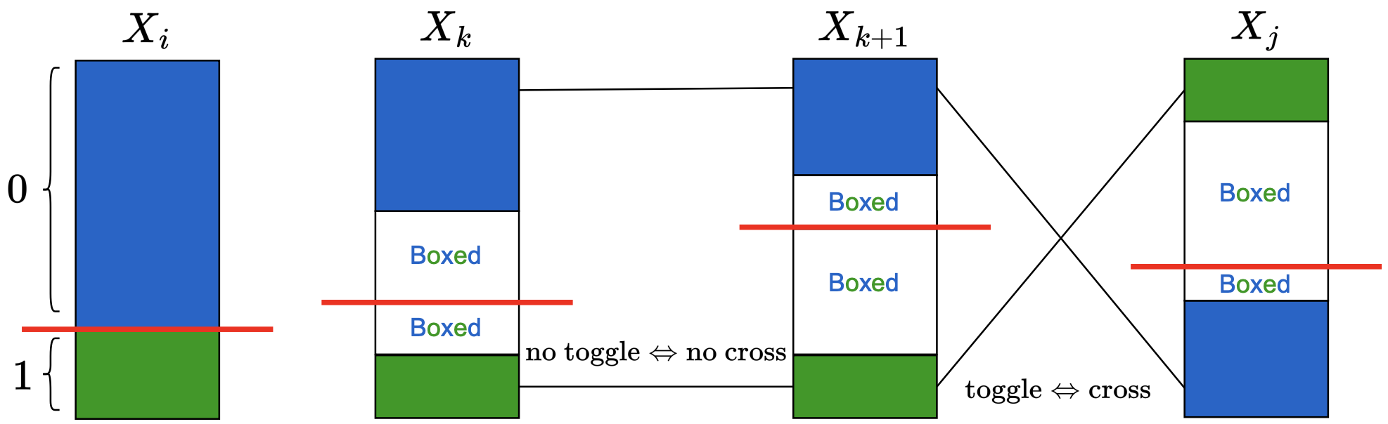
Figure 4: The case where $\operatorname{{Br}}(X_{i}|X_{j})<2\cdot b(i),\frac{1}{2}$. Each $X_{i+1},\dots,X_{j}$ has unmatched blue/green mass in each state, totalling more than $\frac{1}{2}$. The boxed mass in each state has equal green and blue mass. Toggles and crosses are in one-to-one correspondence in this case. In the picture above, we are imagining there to be an odd number of toggles on the path $X_{i}\to X_{j}$. Observe how this results in all of the unmatched mass in $X_{j}$ contributing to $\operatorname{{Pr}}[X_{i}\neq X_{j}]$. In particular, for $X_{j}$ (for which #toggles is odd), $\operatorname{{Pr}}[X_{i}\neq X_{j}]=1-\frac{1}{2}\operatorname{{Br}}[X_{i}|X_{j}]$, while for $X_{k+1}$ (for which #toggles is even), $\operatorname{{Pr}}[X_{i}\neq X_{k+1}]=\frac{1}{2}\operatorname{{Br}}[X_{i}|X_{k+1}]$.

In this case, observe that by Lemma 5.3, for any $X_{k}\in X_{i}\to X_{j}$, $\operatorname{{Br}}(X_{i}|X_{k})<2\cdot b(i),\frac{1}{2}$. In particular, the former inequality means that at every $k$, the two states of $X_{k}$ contain non-zero amounts of different “unmatched” states of $X_{i}$ (refer to Figure 4), and as we move from $X_{k}$ to $X_{k+1}$, the configuration of these unmatched states either toggles (blue-green $\to$ green-blue or green-blue $\to$ blue-green) or stays the same. The latter inequality means that these states further total to $>\frac{1}{2}$ at every $k$. Observe that in this case, the configuration from $X_{k}$ to $X_{k+1}$ toggles if and only if the edge connecting them is a cross. This is because, since the unmatched states amount to a mass $>\frac{1}{2}$, a toggle would mean that $\operatorname{{Pr}}[X_{k}=0,X_{k+1}=1]+\operatorname{{Pr}}[X_{k}=1,X_{k+1}=0]>\frac{1}{2}$, which corresponds to a cross edge. Similarly, a non-toggle would mean that $\operatorname{{Pr}}[X_{k}=0,X_{k+1}=0]+\operatorname{{Pr}}[X_{k}=1,X_{k+1}=1]>\frac{1}{2}$, which is a non-cross edge. Now, if we are given there are an odd number of crosses between $X_{i}$ and $X_{j}$, then that means there are an odd number of toggles, which means that the unmatched states contribute their mass towards $\operatorname{{Pr}}[X_{i}\neq X_{j}]$. Namely, we get $\operatorname{{Pr}}[X_{i}\neq X_{j}]>\frac{1}{2}\geq\min(b(i),b(j))$. ∎

To conclude the proof of the “odd crosses” case, we note that

$$\max(b(i),b(j))=\min(b(i),b(j))+|b(i)-b(j)|=O(\operatorname{{Pr}}[X_{i}\neq X_{j}]),$$

where we used 5.6 and Lemma 5.4. ∎

We aim to show that the sum of the three metrics given in Lemma 5.5 will be an approximation of $\operatorname{{Pr}}[X_{i}\neq X_{j}]$. This would follow from showing:

Lemma 5.7.

Suppose $|\operatorname{{Pr}}[X_{i}=0]-\operatorname{{Pr}}[X_{j}=0]|,\operatorname{{Br}}(X_{i}|X_{j})\leq\frac{1}{100}\cdot\operatorname{{Pr}}[X_{i}\neq X_{j}]$, then it must hold that $b(i),b(j)\in[0.485,0.5]$ and that there are an odd number of crosses between $X_{i}$ and $X_{j}$.

Proof.

Case 1: $\operatorname{{Br}}(X_{i}|X_{j})<2\cdot b(i)$. In this case, as $\operatorname{{Br}}(X_{i}|X_{j})\leq\frac{1}{100}\cdot\operatorname{{Pr}}[X_{i}\neq X_{j}]<\frac{1}{2}$ as well, as depicted in Figure 4, it must hold that $\operatorname{{Pr}}[X_{i}\neq X_{j}]=\frac{1}{2}\cdot\operatorname{{Br}}(X_{i}|X_{j})$ if there are an even number of crosses from $X_{i}$ to $X_{j}$, and $\operatorname{{Pr}}[X_{i}\neq X_{j}]=1-\frac{1}{2}\cdot\operatorname{{Br}}(X_{i}|X_{j})$ if there are an odd number of crosses. In the even case, it would then not hold that $\operatorname{{Br}}(X_{i}|X_{j})\leq\frac{1}{100}\cdot\operatorname{{Pr}}[X_{i}\neq X_{j}]$. Thus, we must be in the odd number of crosses case, and

$$\operatorname{{Pr}}[X_{i}\neq X_{j}]=1-\frac{1}{2}\cdot\operatorname{{Br}}(X_{i}|X_{j})\geq 1-\frac{1}{200}.$$

Without loss of generality, suppose $\operatorname{{Pr}}[X_{i}=0]\geq\operatorname{{Pr}}[X_{i}=1]$ (as in Figure 4 too). Then, we can see that

$$\operatorname{{Pr}}[X_{i}=0,X_{j}=1]\geq\frac{1}{2}\cdot(1-\operatorname{{Br}}(X_{i}|X_{j}))\geq\frac{99}{200}.$$

Accordingly, $\operatorname{{Pr}}[X_{i}=0],\operatorname{{Pr}}[X_{j}=1]\geq\frac{99}{200}$. Moreover, as $|\operatorname{{Pr}}[X_{i}=0]-\operatorname{{Pr}}[X_{j}=0]|\leq\frac{1}{100}$, then

$$\operatorname{{Pr}}[X_{j}=0]\geq\frac{99}{200}-\frac{1}{100}=\frac{97}{200}.$$

Since $\operatorname{{Pr}}[X_{j}=0]\geq\frac{97}{200}$ and $\operatorname{{Pr}}[X_{j}=1]\geq\frac{99}{200}$, it holds that $b(j)\in[0.485,0.5]$. Similarly,

$$\operatorname{{Pr}}[X_{i}=1]\geq\operatorname{{Pr}}[X_{j}=1]-|\operatorname{{Pr}}[X_{i}=0]-\operatorname{{Pr}}[X_{j}=0]|\geq\frac{99}{200}-\frac{1}{100}=0.485.$$

So, $b(i)\in[0.485,0.5]$ too.

Case 2: $\operatorname{{Br}}(X_{i}|X_{j})=2\cdot b(i)$.

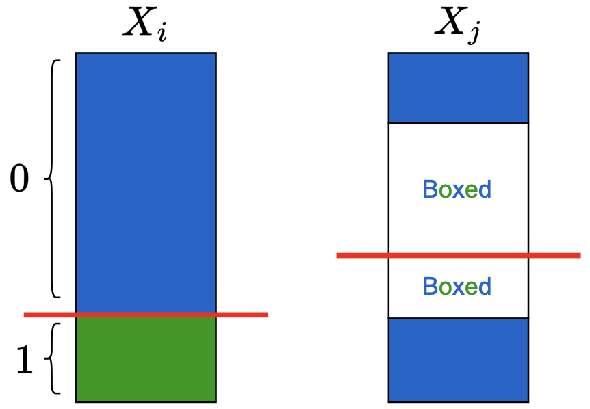
Figure 5: The case where $\operatorname{{Br}}(X_{i}|X_{j})=2\cdot b(i).$ The mass corresponding to the smaller state in $X_{i}$ (green mass) should all be in a box in $X_{j}$.

Without loss of generality assume $\operatorname{{Pr}}[X_{i}=0]\geq\operatorname{{Pr}}[X_{i}=1]$. Since $\operatorname{{Br}}(X_{i}|X_{j})=2\cdot b(i)$, the mass corresponding to the smaller state in $X_{i}$ (Figure 5) must all be in a box in $X_{j}$. This means that

$$\operatorname{{Pr}}[X_{i}\neq X_{j}] \in[\operatorname{{Pr}}[X_{i}=0,X_{j}=1],\operatorname{{Pr}}[X_{i}=1,X_{j}=0]]$$

$$\in\left[\operatorname{{Pr}}[X_{i}=0,X_{j}=1],\frac{1}{2}\cdot\operatorname{{Br}}(X_{i}|X_{j})+\operatorname{{Pr}}[X_{i}=0,X_{j}=1]\right].$$ (13)

Since by assumption, $b(i)=\operatorname{{Pr}}[X_{i}=1]$,

$$\operatorname{{Pr}}[X_{j}=1] \leq\operatorname{{Pr}}[X_{i}=1]+|\operatorname{{Pr}}[X_{i}=1]-\operatorname{{Pr}}[X_{j}=1]|$$

$$=b(i)+|\operatorname{{Pr}}[X_{i}=1]-\operatorname{{Pr}}[X_{j}=1]|$$

$$=b(i)+|\operatorname{{Pr}}[X_{i}=0]-\operatorname{{Pr}}[X_{j}=0]|$$

$$=\frac{1}{2}\cdot\operatorname{{Br}}(X_{i}|X_{j})+|\operatorname{{Pr}}[X_{i}=0]-\operatorname{{Pr}}[X_{j}=0]|$$

$$\leq\frac{2}{100}\cdot\operatorname{{Pr}}[X_{i}\neq X_{j}].$$

But then combining with (5.2), this gives

$$\operatorname{{Pr}}[X_{i}\neq X_{j}] \leq\frac{1}{2}\cdot\operatorname{{Br}}(X_{i}|X_{j})+\operatorname{{Pr}}[X_{i}=0,X_{j}=1]$$

$$\leq\frac{1}{2}\cdot\operatorname{{Br}}(X_{i}|X_{j})+\operatorname{{Pr}}[X_{j}=1]$$

$$\leq\frac{1}{200}\operatorname{{Pr}}[X_{i}\neq X_{j}]+\frac{2}{200}\operatorname{{Pr}}[X_{i}\neq X_{j}]=\frac{3}{200}\operatorname{{Pr}}[X_{i}\neq X_{j}]<\operatorname{{Pr}}[X_{i}\neq X_{j}],$$

which is a contradiction. ∎

Corollary 5.8.

The sum of the three metrics in Lemma 5.5 i.e., $d_{\mathrm{marg}}+d_{\operatorname{{Br}}}+d_{\mathrm{negcor}}$ is a $\Theta(1)$-distortion embedding for $\operatorname{{Pr}}[X_{i}\neq X_{j}]$.

Proof.

By Lemma 5.5, we know that the metrics do not individually overestimate (upto constant factors). Now, we just want to show that their sum does not sufficiently underestimate. If the sum of the metrics was to underestimate under $\frac{1}{100}\cdot\operatorname{{Pr}}[X_{i}\neq X_{j}]$, then the conditions of Lemma 5.7 must hold. However, the result of Lemma 5.7 then implies that the third metric will yield distance $\geq 0.485$, causing a contradiction as the distance of any $\operatorname{{Pr}}[X_{i}\neq X_{j}]\leq 1<100\cdot 0.485$. ∎

Now all that remains is to show that each of the three metrics in Lemma 5.5 can be embedded efficiently into $\ell_{1}$ with constant distortion. The first metric can be embedded exactly into $\ell_{1}$ simply with one coordinate having value $\operatorname{{Pr}}[X_{i}=0]$. The third metric also easily embeds into $\ell_{1}$ by having a single coordinate for each $X_{i}$ which is $b(i)$ if there is an even number of crosses from the root to $X_{i}$, and $-b(i)$ if there is an odd number of crosses from the root to $X_{i}$. For any two nodes $X_{i}$ and $X_{j}$, note that this coordinate measures a distance $|b(i)-b(j)|$ iff there is an even number of crosses on the path between $X_{i}$ and $X_{j}$, and distance $|b(i)+b(j)|\in[\max(b(i),b(j)),2\cdot\max(b(i)+b(j))]$ iff there is an odd number of crosses.

The second metric is the most complicated to embed into $\ell_{1}$. To do so, we once again seek to reduce the task at hand to embedding a capped-tree metric. Recall that in the case of symmetric tree Ising models, we were able to reduce the task to a tree metric with a fixed cap. The more general asymmetric case requires us to be able to embed a tree metric with a Lipschitz cap instead, where the Lipschitzness in the caps is with respect to the tree distance between nodes. More concretely, we consider a tree with the same tree structure as the tree Ising model. We specify edge weights for every edge $e=(X_{u},X_{v})$ in the tree, via a quantity that we call ‘‘forced randomness".

Definition 4 (Forced randomness).

For an edge $e=(X_{u},X_{v})$, its forced randomness $\mathcal{F}_{e}$ is defined as follows: $\mathcal{F}_{e}=\max(\operatorname{{Br}}(X_{u}|X_{v}),\operatorname{{Br}}(X_{v}|X_{u}))$.

Now, we define the following Lipschitz capped-tree metric:

Definition 5 (Forced randomness Lipschitz-capped tree metric).

Every node $X_{i}$ in the tree is associated with a cap $b(i)$. The edge weights are given by $\mathcal{F}_{e}$. The distance is defined as

$$d_{\mathcal{F}}(i,j)=\min\left(\sum_{e\in(i\to j)}\mathcal{F}_{e},\max(b(i),b(j))\right).$$ (14)

Note that the caps respect Lipschitzness with respect to the tree distance.

Claim 5.9.

The forced randomness Lipschitz-capped tree distance is a valid Lipschitz capping because for every $e=(X_{u},X_{v})$ it holds that $|b(u)-b(v)|\leq\mathcal{F}_{e}$.

Proof.

This follows directly from the proof of Lemma 5.4, which asserts that $|b(u)-b(v)|\leq\frac{1}{2}\cdot\mathcal{F}_{e}$. ∎

We show that it suffices to be able to efficiently embed this Lipschitz-cap tree metric into $\ell_{1}$ in order to embed $\operatorname{{Br}}(X_{i}|X_{j})$. First, we show that $d_{\mathcal{F}}(i,j)$ does not vastly underestimate the quantities that we are interested in.

Lemma 5.10 (No underestimation).

Let $d_{\mathcal{F}}(i,j)$ denote the forced randomness Lipschitz-capped tree distance between $X_{i}$ and $X_{j}$. Then, $d_{\mathcal{F}}(i,j)\geq\min(\max(b(i),b(j)),\operatorname{{Br}}(X_{i}|X_{j}))$.

Proof.

Note how this immediately holds if we show that the uncapped distance i.e., $\sum_{e\in(i\to j)}\mathcal{F}_{e}$ is at least $\operatorname{{Br}}(X_{i}|X_{j})$. Recall that

$$\sum_{e=(X_{k},X_{k+1})\in(i\to j)}\mathcal{F}_{e}=\sum_{(X_{k},X_{k+1})\in(i\to j)}\max(\operatorname{{Br}}(X_{k}|X_{k+1}),\operatorname{{Br}}(X_{k+1}|X_{k}))\geq\sum_{(X_{k},X_{k+1})\in(i\to j)}\operatorname{{Br}}(X_{k}|X_{k+1}).$$

Thus, it is sufficient to show:

Claim 5.11.

$\sum_{k:i\rightarrow j}\operatorname{{Br}}(X_{k}|X_{k+1})\geq\operatorname{{Br}}(X_{i}|X_{j})$

Proof.

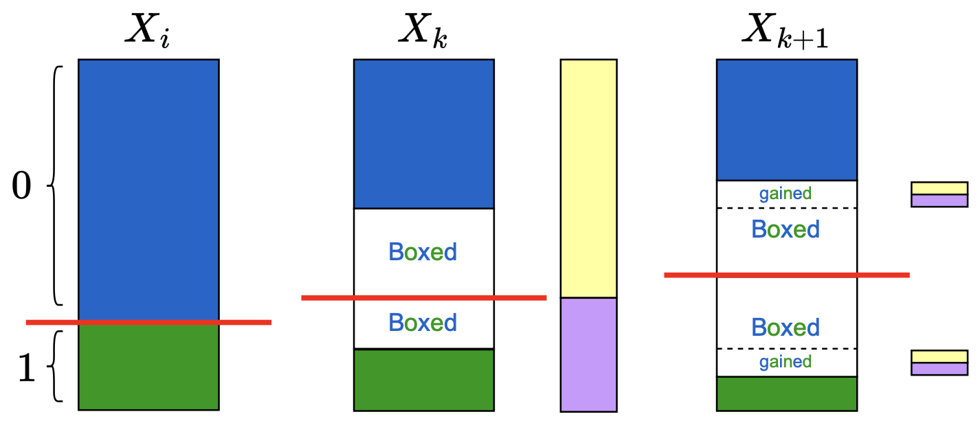
Figure 6: The “blue-green” boxed mass in $X_{k}$ corresponds to $\operatorname{{Br}}[X_{i}|X_{k}]$. The gained blue-green boxed mass in $X_{k+1}$ must come from the unboxed mass from different states in $X_{k}$. Reinterpreting mass in the different states of $X_{k}$ as yellow and purple, we can see that the gained blue-green boxed mass certainly also constitutes yellow-purple boxed mass in $X_{k+1}$, meaning that it forms part of $\operatorname{{Br}}[X_{k}|X_{k+1}]$.

Let the mass in $X_{i}=0$ and $X_{i}=1$ be colored blue and green respectively, as in Figure 6. For any $k:i\to j$, the “blue-green” boxed mass is non-decreasing as we go from $X_{k}$ to $X_{k+1}$ (Lemma 5.3), and $\operatorname{{Br}}[X_{i}|X_{k+1}]-\operatorname{{Br}}[X_{i}|X_{k}]$ is exactly the increase in boxed mass. Observe that any increase in boxed mass at $X_{k+1}$ must come from mass that was unboxed and separate at $X_{k}$. Since this new boxed mass in either state of $X_{k+1}$ was from separate states in $X_{k}$, it also forms part of $\operatorname{{Br}}[X_{k}|X_{k+1}]$. This is made clear if we think of all the mass under $\operatorname{{Pr}}[X_{k}=0]$ as yellow, and all the mass under $\operatorname{{Pr}}[X_{k}=1]$ as purple, so that any additional blue-green boxed mass in $X_{k+1}$ is in fact also yellow-purple boxed mass. Thus, we have argued that $\operatorname{{Br}}[X_{i}|X_{k+1}]-\operatorname{{Br}}[X_{i}|X_{k}]\leq\operatorname{{Br}}[X_{k}|X_{k+1}]$. Since this holds for every $k=i,i+1,\dots,j-1$, we can add up the inequalities to obtain a telescoping sum as follows:

$$\sum_{k:i\to j}\left(\operatorname{{Br}}[X_{i}|X_{k+1}]-\operatorname{{Br}}[X_{i}|X_{k}]\right)=\operatorname{{Br}}[X_{i}|X_{j}]-\operatorname{{Br}}[X_{i}|X_{i}]=\operatorname{{Br}}[X_{i}|X_{j}]\leq\sum_{k:i\to j}\operatorname{{Br}}[X_{k}|X_{k+1}].$$

∎

∎

Second, and finally, we will show that this metric does not overestimate above $O(\operatorname{{Pr}}[X_{i}\neq X_{j}])$.

Lemma 5.12 (No overestimation).

Let $d_{\mathcal{F}}(i,j)$ denote the forced randomness Lipschitz-capped tree distance between $X_{i}$ and $X_{j}$. Then, $d_{\mathcal{F}}(i,j)\leq 200\cdot\operatorname{{Pr}}[X_{i}\neq X_{j}]$.

Proof.

Let $\mathcal{S}_{ij}$ be the set of edges $(X_{k},X_{k+1})$ on the path from $i$ to $j$ for which $\operatorname{{Br}}(X_{k}|X_{k+1})\geq\operatorname{{Br}}(X_{k+1}|X_{k})$, and let $S_{ji}$ be the set of edges for which $\operatorname{{Br}}(X_{k}|X_{k+1})<\operatorname{{Br}}(X_{k+1}|X_{k})$.

Let us first process edges in $S_{ij}$. Suppose $\max(b(i),b(j))>100\cdot\operatorname{{Pr}}[X_{i}\neq X_{j}]$ and $\sum_{e\in S_{ij}}\mathcal{F}_{e}>100\cdot\operatorname{{Pr}}[X_{i}\neq X_{j}]$.
Case 1: $\operatorname{{Br}}(X_{i}|X_{k})<\min\left(\frac{99}{100}b(i),\frac{1}{2}b(k)\right)$ for every $e=(X_{k},X_{k+1})\in S_{ij}.$

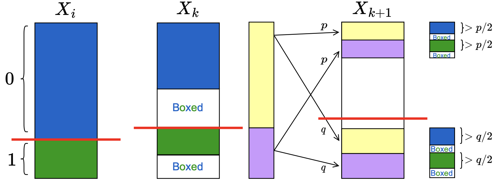
Figure 7: We reinterpret mass in the different states of $X_{k}$ as yellow and purple. The total “yellow-purple” boxed mass in both states of $X_{k+1}$ constitutes $\operatorname{{Br}}[X_{k}|X_{k+1}]$. The gained blue-green boxed mass in $X_{k+1}$ must come from unboxed mass from different states in $X_{k}$. Under the assumption that $\operatorname{{Br}}(X_{i}|X_{k})<\min\left(\frac{99}{100}b(i),\frac{1}{2}b(k)\right)$, at least half of $\operatorname{{Br}}[X_{k}|X_{k+1}]$ is derived from unboxed blue-green mass in $X_{k}$.

Consider any $e=(X_{k},X_{k+1})\in S_{ij}$. Refer to Figure 7. Since $\operatorname{{Br}}(X_{i}|X_{k})<\frac{99}{100}b(i)<2b(i)$, there must be different-colored unboxed mass overflowing in each state of $X_{k}$. As mentioned previously in the proof of 5.11, $\operatorname{{Br}}[X_{i}|X_{k+1}]-\operatorname{{Br}}[X_{i}|X_{k}]$ is exactly the increase in “blue-green” boxed mass as we go from $X_{k}$ to $X_{k+1}$, and this increase in boxed mass must come from mass that was unboxed and separate at $X_{k}$. With a view to reason about $\operatorname{{Br}}[X_{k}|X_{k+1}]$, let us reinterpret the mass in state 0 at $X_{k}$ as yellow and that in state 1 as purple. Then, $\operatorname{{Br}}[X_{k}|X_{k+1}]$ is precisely the total “yellow-purple” boxed mass across both states of $X_{k+1}$. In the figure, $\operatorname{{Br}}[X_{k}|X_{k+1}]=2p+2q$, corresponding to a $p$ amount of mass coming from each state of $X_{k}$ into state 0 of $X_{k+1}$, and a $q$ amount of mass coming from each state of $X_{k}$ into state 1 of $X_{k+1}$. But recall that because of the Markov property, the proportion of blue and green mass in, say the $p$ amount of yellow mass coming from state $``X_{k}=0"$ into state $``X_{k+1}=0"$ is the same as it was in all of state $``X_{k}=0"$. Since we are also assuming that $\operatorname{{Br}}[X_{i}|X_{k}]<\frac{1}{2}b(k)$, this means that at least one half of the yellow mass constituting $\operatorname{{Br}}[X_{k}|X_{k+1}]$ in state $``X_{k+1}=0"$ corresponds to unboxed blue mass. Similarly, at least one half of the purple mass constituting $\operatorname{{Br}}[X_{k}|X_{k+1}]$ in state $``X_{k+1}=0"$ corresponds to unboxed green mass. This means that we have at least $\frac{p}{2}+\frac{p}{2}=p$ new boxed blue-green mass in state 0 of $X_{k+1}$ arising out of previously unboxed blue-green mass in $X_{k}$. The same holds true for the state $X_{k+1}$, where we have at least $\frac{q}{2}+\frac{q}{2}=q$ new boxed blue-green mass arising out of unboxed mass in $X_{k}$. In total, we have at least $p+q\geq\frac{1}{2}\operatorname{{Br}}[X_{k}|X_{k+1}]$ new boxed blue-green mass in $X_{k+1}$ arising out of unboxed mass in $X_{k}$, meaning, from our earlier reasoning and the definition of $\mathcal{F}_{e}$ for $e\in S_{ij}$, that

$$\operatorname{{Br}}[X_{i}|X_{k+1}]-\operatorname{{Br}}[X_{i}|X_{k}]\geq\frac{1}{2}\operatorname{{Br}}[X_{k}|X_{k+1}]=\frac{1}{2}\mathcal{F}_{e}.$$

Under the current case, this logic holds for every $e=(X_{k},X_{k+1})\in S_{ij}$, which means that

$$\frac{1}{2}\sum_{e\in S_{ij}}\mathcal{F}_{e} \leq\sum_{e=(X_{k},X_{k+1})\in S_{ij}}\operatorname{{Br}}(X_{i}|X_{k+1})-\operatorname{{Br}}(X_{i}|X_{k})$$

$$\leq\sum_{k:i\to j}\operatorname{{Br}}(X_{i}|X_{k+1})-\operatorname{{Br}}(X_{i}|X_{k})$$

$$=\operatorname{{Br}}[X_{i}|X_{j}]$$

$$\leq 2\operatorname{{Pr}}[X_{i}\neq X_{j}]$$

$$<\frac{1}{50}\sum_{e\in S_{ij}}\mathcal{F}_{e}$$

which is a contradiction.

Thus, it must be the case that $\operatorname{{Br}}(X_{i}|X_{k})\geq\min\left(\frac{99}{100}b(i),\frac{1}{2}b(k)\right)$ for some $e=(X_{k},X_{k+1})\in S_{ij}.$ Now, observe that under our assumptions and by Lemma 5.4,

$$|b(i)-b(j)|\leq\operatorname{{Pr}}[X_{i}\neq X_{j}]<\frac{1}{100}\max(b(i),b(j)).$$ (15)

Therefore,

$$b(i)\geq\max(b(i),b(j))-|b(i)-b(j)|>\frac{99}{100}\max(b(i),b(j)).$$ (16)

Case 2: $\operatorname{{Br}}(X_{i}|X_{k})\geq\frac{99}{100}b(i)$ for some $e=(X_{k},X_{k+1})\in S_{ij}$.

If $\operatorname{{Br}}(X_{i}|X_{k})\geq\frac{99}{100}b(i)$, we would have

$$\operatorname{{Pr}}[X_{i}\neq X_{j}] \geq\frac{1}{2}\operatorname{{Br}}[X_{i}|X_{j}]$$

$$\geq\frac{1}{2}\operatorname{{Br}}[X_{i}|X_{k}]\qquad(\text{\lx@cref{creftypecap~refnum}{lemma:data-processing-inequality}})$$

$$\geq\frac{1}{2}\cdot\frac{99}{100}b(i)$$

$$>\frac{1}{2}\cdot\left(\frac{99}{100}\right)^{2}\max(b(i),b(j))\qquad(\text{from }\eqref{eqn:bi-bound})$$

$$>\operatorname{{Pr}}[X_{i}\neq X_{j}],$$

which is a contradiction.

Case 3: $\operatorname{{Br}}(X_{i}|X_{k})\geq\frac{1}{2}b(k)$ but $\operatorname{{Br}}(X_{i}|X_{k})<\frac{99}{100}b(i)$ for some $e=(X_{k},X_{k+1})\in S_{ij}$.
If $b(k)\geq\frac{1}{5}b(i)$, then we would have

$$\operatorname{{Pr}}[X_{i}\neq X_{j}] \geq\frac{1}{2}\operatorname{{Br}}[X_{i}|X_{k}]\geq\frac{1}{4}b(k)\geq\frac{1}{20}b(i)>\frac{1}{20}\cdot\frac{99}{100}\max(b(i),b(j))>\operatorname{{Pr}}[X_{i}\neq X_{j}],$$

which is a contradiction.
On the other hand, if $b(k)<\frac{1}{5}b(i)$, we would have

$$\operatorname{{Pr}}[X_{i}\neq X_{j}] \geq\frac{1}{2}\operatorname{{Br}}[X_{i}|X_{k}]$$

$$\geq b(i)-b(k)\qquad(\text{\lx@cref{creftypecap~refnum}{lemma:br-bound}})$$

$$>\frac{4}{5}b(i)>\frac{4}{5}\cdot\frac{99}{100}\max(b(i),b(j))>\operatorname{{Pr}}[X_{i}\neq X_{j}],$$

which is again contradiction.

Thus, we have shown that if both $\max(b(i),b(j))>100\cdot\operatorname{{Pr}}[X_{i}\neq X_{j}]$ and $\sum_{e\in S_{ij}}\mathcal{F}_{e}>100\cdot\operatorname{{Pr}}[X_{i}\neq X_{j}]$, every possible case leads to a contradiction. Consequently, it must be true that

$$\min\left(\max(b(i),b(j)),\sum_{e\in S_{ij}}\mathcal{F}_{e}\right)\leq 100\cdot\operatorname{{Pr}}[X_{i}\neq X_{j}].$$ (17)

Repeating the argument above for edges $e\in S_{ji}$ gives

$$\min\left(\max(b(i),b(j)),\sum_{e\in S_{ji}}\mathcal{F}_{e}\right)\leq 100\cdot\operatorname{{Pr}}[X_{i}\neq X_{j}].$$ (18)

The lemma follows by putting (17) and (18) together, and using

$$d_{\mathcal{F}}(i,j) =\min\left(\max(b(i),b(j)),\sum_{e\in(i\to j)}\mathcal{F}_{e}\right)$$

$$=\min\left(\max(b(i),b(j)),\sum_{e\in S_{ij}}\mathcal{F}_{e}+\sum_{e\in S_{ji}}\mathcal{F}_{e}\right)$$

$$\leq\min\left(\max(b(i),b(j)),\sum_{e\in S_{ij}}\mathcal{F}_{e}\right)+\min\left(\max(b(i),b(j)),\sum_{e\in S_{ji}}\mathcal{F}_{e}\right)$$

$$\leq 200\cdot\operatorname{{Pr}}[X_{i}\neq X_{j}].$$

∎

Therefore, we have shown that the forced randomness Lipschitz cap tree metric neither grossly underestimates nor overestimates. This lets us substitute $d_{\mathcal{F}}$ for $d_{\operatorname{{Br}}}$ in Corollary 5.8.

Corollary 5.13.

The sum $d_{\mathrm{marg}}+d_{\mathcal{F}}+d_{\mathrm{negcor}}$ is a $\Theta(1)$-distortion embedding for $\operatorname{{Pr}}[X_{i}\neq X_{j}]$.

Proof.

Fix nodes $X_{i}$ and $X_{j}$. From Corollary 5.8, we know that

$$\Theta(1)\cdot\operatorname{{Pr}}[X_{i}\neq X_{j}]\leq d_{\mathrm{marg}}(i,j)+d_{\operatorname{{Br}}}(i,j)+d_{\mathrm{negcor}}(i,j)\leq\Theta(1)\cdot\operatorname{{Pr}}[X_{i}\neq X_{j}].$$ (19)

This gives

$$d_{\mathrm{marg}}(i,j)+d_{\mathcal{F}}(i,j)+d_{\mathrm{negcor}}(i,j) \leq d_{\mathrm{marg}}(i,j)+100\cdot\operatorname{{Pr}}[X_{i}\neq X_{j}]+d_{\mathrm{negcor}}(i,j)\qquad(\text{\lx@cref{creftypecap~refnum}{lemma:forced-radomness-no-overestimate}})$$

$$\leq\Theta(1)\cdot(d_{\mathrm{marg}}(i,j)+d_{\operatorname{{Br}}}(i,j)+d_{\mathrm{negcor}}(i,j))\qquad(\text{lower bound in \eqref{eqn:good-metrics-to-modified-good-metrics}})$$

$$\leq\Theta(1)\cdot\operatorname{{Pr}}[X_{i}\neq X_{j}]\qquad(\text{upper bound in \eqref{eqn:good-metrics-to-modified-good-metrics}}).$$

Next, from Lemma 5.10, we know that

$$d_{\mathcal{F}}(i,j)\geq\min(\max(b(i),b(j)),\operatorname{{Br}}[X_{i}|X_{j}]).$$

But notice that

$$\max(b(i),b(j)) \geq b(i)\geq\frac{1}{2}\operatorname{{Br}}[X_{i}|X_{j}],$$

and hence

$$d_{\mathcal{F}}(i,j)\geq\min(\max(b(i),b(j)),\operatorname{{Br}}[X_{i}|X_{j}])\geq\frac{1}{2}\operatorname{{Br}}[X_{i}|X_{j}]=\frac{1}{2}d_{\operatorname{{Br}}}(i,j).$$

Finally,

$$d_{\mathrm{marg}}(i,j)+d_{\mathcal{F}}(i,j)+d_{\mathrm{negcor}}(i,j) \geq d_{\mathrm{marg}}(i,j)+\frac{1}{2}d_{\operatorname{{Br}}}(i,j)+d_{\mathrm{negcor}}(i,j)$$

$$\geq\frac{1}{2}\left(d_{\mathrm{marg}}(i,j)+d_{\operatorname{{Br}}}(i,j)+d_{\mathrm{negcor}}(i,j)\right)$$

$$\geq\Theta(1)\cdot\operatorname{{Pr}}[X_{i}\neq X_{j}]\qquad(\text{lower bound in \eqref{eqn:good-metrics-to-modified-good-metrics}}).$$

∎

In summary, we have shown that if we are able to efficiently embed the forced randomness Lipschitz cap tree metric $d_{\mathcal{F}}$ efficiently into $\ell_{1}$ with constant distortion, we will have achieved our goal of embedding $\operatorname{{Pr}}[X_{i}\neq X_{j}]$ into $\ell_{1}$ (recall that $d_{\mathrm{marg}}$ and $d_{\mathrm{negcor}}$ embed into $\ell_{1}$ in a very simple manner). In the following section, we show that Lipschitz cap tree metrics embed into $\ell_{1}$ with only $O(\log^{2}(n))$ dimensions.

5.3 Lipschitz Cap Metrics

As before, we begin our journey on Lipschitz cap metrics with the basic case of a line graph metric. As it turns out, the technique of lazy snaking that we used for the fixed cap line ends up being sufficient for the Lipschitz cap case, with a slight modification.

5.3.1 Lipschitz Cap Line Metrics

Let $L_{n}$ be the line graph on $n$ vertices $x_{1},\dots,x_{n}$, where each pair of consecutive vertices $x_{i},x_{i+1}$ is connected by an edge of length $e_{i}\in\mathds{Z}_{>0}$, and $d(x_{i},x_{j})=\sum_{k=i}^{j-1}e_{i}$. Let $loc[i]=d(x_{i},x_{1})$. Throughout what follows, we will identify every vertex $x_{i}$ with $loc[i]$ instead. Every vertex has associated with it a cap, given by the cap function $M:\mathds{R}\to\mathds{Z}_{\geq 0}$, so that the cap at vertex $x_{i}$ is $M(loc[i])$. The cap function $M$ satisfies the Lipschitz property in the graph distance, i.e., for any $i,j$, $|M(loc[i])-M(loc[j])|\leq|loc[i]-loc[j]|$. Let $loc[0]=-2M(0)$, and for any $i\geq 0$, $t\in[loc[i],loc[i+1]]$, let us additionally define $M(t)$ to be the linear interpolation of $M(loc[i])$ and $M(loc[i+1])$ i.e., $M(t)=M(loc[i])+\left(\frac{M(loc[i+1])-M(loc[i])}{loc[i+1]-loc[i]}\right)\cdot(t-loc[i])$. Consider the metric space $(L_{n},d^{{M}}_{\mathrm{lipcap}})$ equipped with the Lipschitz cap line metric, defined as

$$d^{{M}}_{\mathrm{lipcap}}(x_{i},x_{j})=\min(d(x_{i},x_{j}),\max(M(loc[i]),M(loc[j])).$$ (20)

Given that we have a different cap value at every node, a natural idea, and intuitive generalization of the lazy snaking procedure in Algorithm 1 would be to snake around with varying widths depending on the cap function. In fact, this modification is sufficient for our purposes, and is described in Algorithm 2.

Algorithm 2 Lazy Snaking for Lipschitz-cap line metric

Input: List of $n$ node locations $loc[]$, Lipschitz cap function $M$

Output: List of embeddings for the nodes $embedding[]$

1:procedure LipschitzLazySnake($loc,M$):

2:      $t\leftarrow-2M(0)$

3:     while $t\leq loc[n]$ do

4:         $\Delta\sim\mathrm{Uniform}\{0,1\}$

5:         if $\Delta=0$ then $\triangleright$ Rest for a duration $\frac{M(t)}{300}$

6:              $snake[t^{\prime}]\leftarrow 0$ for $t^{\prime}\in\left[t,t+\frac{M(t)}{300}\right]$

7:              $t\leftarrow t+\frac{M(t)}{300}$

8:         end if

9:         if $\Delta=1$ then $\triangleright$ Snake with a width $\frac{M(t)}{100}$

10:              $snake[t^{\prime}]=t^{\prime}-t$ for $t^{\prime}\in\left[t,t+\frac{M(t)}{100}\right]$

11:              $snake[t^{\prime}]=\frac{2M(t)}{100}-(t^{\prime}-t)$ for $t^{\prime}\in\left[t+\frac{M(t)}{100},t+\frac{2M(t)}{100}\right]$

12:              $t\leftarrow t+\frac{2M(t)}{100}$

13:         end if

14:     end while

15:     for $i\leftarrow 1$ to $n$ do

16:         $embedding[i]=snake[loc[i]]$

17:     end for

18:     return $embedding[]$

19:end procedure

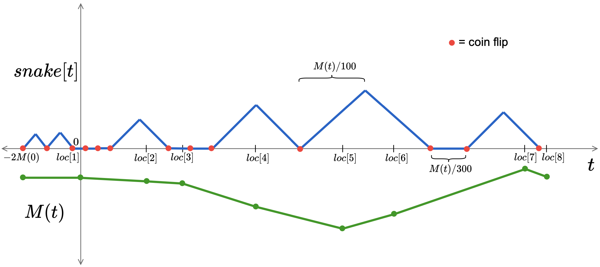
Figure 8: Lazy snaking with Lipschitz cap.

We remark that Algorithm 1 and Algorithm 2 are nearly identical, except for constants and initialization. The modified initialization is necessary for algorithm correctness when the cap is non-constant, for a technical reason.

Just like 4.4, we have the guarantee that for every pair of nodes, Algorithm 2 does not overestimate their distance, and also covers at least a constant fraction of it in expectation.

Lemma 5.14.

Let $M$ be a strictly positive function, and let $embedding=\textsc{LipschitzLazySnake}(loc,M)$. For every fixed pair of nodes $x_{i}$ and $x_{j}$,

$$\text{(1) }\operatorname{{Pr}}\left[\|embedding[i]-embedding[j]\|_{1}\leq d^{{M}}_{\mathrm{lipcap}}(x_{i},x_{j})\right]=1.$$

$$\text{(2) }\operatorname{{\mathds{E}}}\left[\|embedding[i]-embedding[j]\|_{1}\right]\geq\Omega(1)\cdot d^{{M}}_{\mathrm{lipcap}}(x_{i},x_{j}).$$

Proof.

The proof mirrors the proof of 4.4 stepwise (although with slightly messier calculations), and is given in Appendix A. ∎

Boosting the above in-expectation guarantee using logarithmically many dimensions then yields the following theorem:

Theorem 6 (Lipschitz cap line into $\ell_{1}$).

$(L_{n},d^{{M}}_{\mathrm{lipcap}})$ can be embedded into $(\mathds{R}^{d},\ell_{1})$ where $d=O(\log n)$ with $\Theta(1)$ distortion.

5.3.2 Lipschitz Cap Tree Metrics

We will now consider how to obtain the analogous result for Lipschitz cap tree metrics. It is tp tempting to try and combine our techniques from the fixed cap tree metric and our Lipschitz cap line metric. Recall how our main technique for the fixed cap tree metric was to obtain a modified ‘‘snipped" version of the tree’s caterpillar decomposition and to reduce (by hashing) the embedding problem to a collection of fixed cap line metric problems. However, we cannot reduce the Lipschitz cap tree metric to a collection of Lipschitz cap line metrics in an obvious manner. Crucially, a direct modification of the prior approach would not work for Lipschitz cap tree metrics, primarily because segments that are hashed to a line metric instance are not contiguous segments of the tree, and thus the caps on these segments need no longer satisfy the necessary Lipschitz condition. Consequently, we must design a new algorithm for this task.

Algorithm Intuition. First, we observe that the primary issue in extending our prior techniques was how tree edges hashed to the same line metrics potentially have very different caps. If we view the algorithm hierarchically (considering how the embedding evolves as we progress downwards in the tree), it would be desirable to ‘‘clean’’/zero out the embedding somehow. If we clean the embedding frequently enough, we may expect that the only edges affecting some $embedding[x_{i}]$ would be parts of the tree very close to $x_{i}$, and thus by the Lipschitz property, all the relevant edges would have roughly the same cap. Ultimately, we obtain an algorithm that is less directly similar to the previous approaches, but is conducive towards this notion of periodic cleaning.

Build-Clean-Tree Algorithm. We now define our ‘‘Build-Clean-Tree" algorithm.

Tree decomposition. We will again consider a modified caterpillar decomposition. Abusing notation slightly, we will refer to the caterpillars/segments given by the caterpillar decomposition as edges themselves. For any edge $e$ in the tree decomposition, we will denote $s(e)$ to be the location of the ‘‘start’’ (or top) of the edge, $\ell(e)$ the length of the edge, and $a(e)$ will store an auxiliary value for the edge we will later define. After obtaining the original caterpillar decomposition, we will split up any overly long edges. More concretely, we chop off any edge $e$ having length larger than $\frac{M(s(e))}{100\log(n)}$ at $\frac{M(s(e))}{100\log(n)}$, and then recursively continue chopping the remaining part of the edge. This process ensures that the length of every (potentially chopped) edge $e$ is at most $\frac{M(s(e))}{100\log(n)}$. From this decomposition, we will create the embedding. All embeddings will be of length $|H|=8\log(n)$. Consider building the embedding from the top to bottom, in a way such that we will only process an edge $e$ after its parent has been processed. We will then determine the embedding for everything along the edge $e$ as purely a function of: $embedding(s(e))$ (this is already calculated because the embedding has been calculated for everything along the parent edge), the length $\ell(e)$, and auxiliary information $a(e)$. Our algorithm will work in stages that we call ‘‘building’’ and ‘‘cleaning’’, and the auxiliary information $a(e)$ will store what determines the current stage.

Building. One stage of our algorithm is building. If we process an edge $e$ while the auxiliary information $a(e)$ indicates it is the building stage, we will then uniformly at random determine a hash for the edge $h(e)\in[8\log(n)]$. Let $embedding[i](k)$ denote the $k^{\text{th}}$ coordinate of the embedding at location $i$. Then, we will proceed as follows:

• If $embedding[s(e)](h(e))=0$, then we will walk in the positive direction for the coordinate $h(e)$ as traversing the edge. More formally, suppose $embedding[s(e)+v]$ denotes the embedding at $v$ below $s(e)$ for $v\in[0,\ell(e)]$. Then, we set $embedding[s(e)+v](h(e))=v$. All other coordinates remain the same as $embedding[s(e)]$.

• Otherwise, if $embedding[s(e)](h(e))\neq 0$, then we do nothing and keep the embedding entirely the same as $embedding[s(e)]$.

Note how this process is Lipschitz in how the embedding changes while moving along the tree, and is designed in a way such that we are trying to keep coordinates of the embedding to be at most $O(\frac{M(s(e))}{\log(n)})$ by leveraging properties of our tree decomposition that limits the sizes of edges.

Cleaning. The other stage of our algorithm is cleaning. When we are in a cleaning stage, it is our hope to try make the state closer to $0$, but we must do so in a Lipschitz manner. Accordingly, our algorithm will be to use the edge to walk a coordinate negatively towards $0$. We proceed by:

• If $embedding[s(e)](k)=0$ for all $k$, then do nothing and keep the embedding the same as $embedding[s(e)]$.

• Otherwise, let $k^{*}$ denote the smallest $k$ such that $embedding[s(e)](k^{*})>0$. Then, we will walk negatively for a length of $\min(embedding[s(e)](k^{*}),\ell(e))$. More formally, we set $embedding[s(e)+v](k^{*})=embedding[s(e)](k^{*})-v$ for $v\in[0,\min(embedding[s(e)](k^{*}),\ell(e))]$

Controlling stages. We will design our stages such that build stages process $L_{\textrm{build}}=4\log(n)$ edges, and clean stages process $L_{\textrm{clean}}=9\log(n)$ edges, and we alternate between building and cleaning. Our auxiliary information $a(e)$ will actually be an integer counter $\in\{0,\dots,L_{\textrm{build}}+L_{\textrm{clean}}-1\}$, such that the edge will be processed in the build stage if $a(e)\in\{0,\dots,L_{\textrm{build}}-1\}$ and otherwise in the clean stage if $a(e)\in\{L_{\textrm{build}},\dots,L_{\textrm{build}}+L_{\textrm{clean}}-1\}$. Moreover, $a(e)$ will simply be $a(par(e))+1\mod(L_{\textrm{build}}+L_{\textrm{clean}})$.

Initialization. For technical reasons similar to those of the Lipschitz cap line metric, we will modify the tree so that the root $r$ of the original tree actually has a parent that is a new node $r_{0}$, where $M(r_{0})=M(r)$ and the length of the edge $(r_{0},r)$ is $2M(r)$. We initialize $embedding[r_{0}]=0^{|H|}$. The auxiliary information of the topmost edge in the tree which contains the extra node $r_{0}$ is initialized uniformly at random in $\{0,\dots,L_{\textrm{build}}+L_{\textrm{clean}}-1\}$.

These are the main components of our algorithm.

Analysis intuition. Recall how our tree composition will limit the length of an edge to be $O(\frac{M(s(e))}{\log(n)})$. We will set the length of our stages $L_{\textrm{build}},L_{\textrm{clean}}=\Theta(\log(n))$. With correctly chosen parameters, we can ensure properties such as the following:

• At the end of every clean stage, the embedding is exactly $0$ for every coordinate.

• Leveraging how often we clean, we can show that for any location $x$ it must hold $embedding[x](k)=O\left(\frac{M(x)}{\log(n)}\right)$ for all indices $k$.

• Moreover, using how the embedding is always updated in a Lipschitz manner, and how $\|embedding[x]\|_{1}$
  $=O(M(x))$ by the previous fact, the embeddings never overestimate distances by more than a constant factor, or more formally $\|embedding[x_{i}]-embedding[x_{j}]\|_{1}\leq d^{{M}}_{\mathrm{lipcap}}(x_{i},x_{j})$.

• By analyzing casework, we can also show how this embedding captures at least a constant fraction of the correct distance in expectation.

The main thrust of our proof will focus on a special case where all caps are strictly positive, and then we will reduce the general case to the special case. For what follows, let us assume that $M(x)>0$ at all locations $x$ in the tree. Here again, we have linearly interpolated the cap function $M$ to assign cap values at all points across any edge $(x_{i},x_{j})$ based on cap values at the endpoints $M(x_{i})$ and $M(x_{j})$.

We begin by proving a useful property for our Lipschitz cap trees, that the caps of nearby parts of the tree must have similar caps. For the simplest version of this, we claim about the similarity between points on an edge:

Claim 5.15 (Caps on an edge are close by).

For any edge $e=(u,w)$ in the decomposition with $u=s(e)$ and location $v$ along $e$, it must hold that $\frac{M(u)}{M(v)},\frac{M(v)}{M(u)}\leq 1+\frac{1}{50\log(n)}$.

Proof.

By Lipschitzness, we have that

$$|M(u)-M(v)|\leq\ell(e)\leq\frac{M(u)}{100\log(n)}$$ (21)

$$\implies\left(1-\frac{1}{100\log(n)}\right)M(u)\leq M(v)\leq\left(1+\frac{1}{100\log(n)}\right)M(u)$$ (22)

$$\implies\frac{M(u)}{M(v)},\frac{M(v)}{M(u)}\leq\max\left(1+\frac{1}{100\log(n)},\frac{1}{1-\frac{1}{100\log(n)}}\right)$$ (23)

$$=\max\left(1+\frac{1}{100\log(n)},1+\frac{1}{100\log(n)\left(1-\frac{1}{100\log(n)}\right)}\right)$$ (24)

$$=1+\frac{1}{100\log(n)\left(1-\frac{1}{100\log(n)}\right)}\leq 1+\frac{1}{50\log(n)}.$$ (25)

The last line holds when $\frac{1}{100\log(n)}\leq\frac{1}{2}$, which holds for $n\geq 2$. ∎

This similarly lets us prove claims about the similarity in the caps at starts of edges that are somewhat close:

Claim 5.16 (Caps on a path are close by).

Consider a sequence of edges $e_{1},\dots,e_{k}$, such that each $e_{i},e_{i+1}$ is adjacent (meaning they share a vertex), and $x_{1}$ is on $e_{1}$ and $x_{k}$ is on $e_{k}$. Then, it must hold that $\frac{M(x_{k})}{M(x_{1})}\leq e^{\frac{k}{50\log(n)}}$. As a special case, $\frac{M(s(e_{k}))}{M(s(e_{1}))}\leq e^{\frac{k}{50\log(n)}}$.

Proof.

Note how the adjacency condition in the sequence $e_{1},\dots,e_{k}$ implies that it is possible to traverse from $x_{1}$ to $x_{k}$ by crossing at most $k$ edges. Thus, by 5.15 it holds that:

$$\frac{M(x_{k})}{M(x_{1})} =\frac{M(x_{k})}{M(s(e_{k}))}\cdot\frac{M(s(e_{k}))}{M(s(e_{k-1}))}\cdot\dots\cdot\frac{M(s(e_{3}))}{M(s(e_{2}))}\cdot\frac{M(s(e_{2}))}{M(x_{1})}$$ (26)

$$\leq\left(1+\frac{1}{50\log(n)}\right)^{k}$$ (27)

$$\leq e^{\frac{k}{50\log(n)}},$$ (28)

where in the last step, we used $1+x\leq e^{x}$ for all real $x$. ∎

Intuitively, this claim will enable us to relate the lengths of almost all nearby edges, as on any root-to-leaf path, it will hold that all but $\leq\log(n)$ edges satisfy $\ell(e)=\frac{M(s(e))}{100\log(n)}$. This is because every edge $e$ on a root-to-leaf path that has length smaller than $\frac{M(s(e))}{100\log(n)}$ must either correspond to a whole short caterpillar, or be the last piece of a caterpillar, and there are at most $\log(n)$ caterpillars on any root-to-leaf path.

Next, we will prove a useful property about the cleaning stage---after an entire clean stage, the embedding is exactly $0^{|H|}$:

Claim 5.17 (Complete cleaning).

At time $x$ immediately after processing an entire clean stage (i.e., the last $L_{\textrm{clean}}$ edges were “clean” edges), $embedding[x]=0^{|H|}$.

Proof.

Suppose this invariant holds at the end of every complete clean stage before the clean stage we are currently considering (or at initialization, if there is none.) Then, at the start of this clean stage, any coordinate that is nonzero must be exactly $\ell(e_{\mathcal{B}})$ for one of the at most $L_{\textrm{build}}$ “build” edges $e_{\mathcal{B}}$ in the immediately preceding build stage—namely, there are at most $L_{\textrm{build}}$ such nonzero coordinates. We aim to show that there are at least $2L_{\textrm{build}}$ edges with weight $\geq\max_{e_{\mathcal{B}}}\frac{\ell(e_{\mathcal{B}})}{2}$ in the clean stage, as this would immediately imply that all coordinates were cleaned. To show this, note how, by definition of the modified tree decomposition and the caterpillar property, all but $\log(n)$ of the edges $e_{\mathcal{C}}$ in the clean stage must exactly satisfy $\ell(e_{\mathcal{C}})=\frac{M(s(e_{\mathcal{C}}))}{100\log(n)}$. Moreover, for any $e_{\mathcal{B}}$, $\ell(e_{\mathcal{B}})\leq\frac{M(s(e_{\mathcal{B}}))}{100\log(n)}$. Then, note how any build edge $e_{\mathcal{B}}$ is within a path of length $L_{\textrm{build}}+L_{\textrm{clean}}$ of each clean edge $e_{\mathcal{C}}$, and so by 5.16,

$$\frac{M(s(e_{\mathcal{B}}))}{M(s(e_{\mathcal{C}}))}\leq e^{\frac{L_{\textrm{build}}+L_{\textrm{clean}}}{50\log(n)}}\leq e^{13/50}\leq 2.$$

Thus, at least $L_{\textrm{clean}}-\log(n)=8\log(n)\geq 2L_{\textrm{build}}$ many “clean” edges have length that is at least half of every build edge $e_{\mathcal{B}}$. ∎

As the embedding is regularly cleaned, we use this to show that the $\ell_{1}$ norm of the embedding at any location $x$ is not too large:

Claim 5.18 (Embedding has small norm).

At any location $x$, $\|embedding[x]\|_{1}\leq\frac{M(x)}{2}.$

Proof.

By 5.17, any nonzero coordinate of $embedding[x]$ must correspond to one of the $L_{\textrm{build}}$ build edges among the previous $L_{\textrm{build}}+L_{\textrm{clean}}$ edges processed. Any of the at most $L_{\textrm{build}}$ build edges $e$ must satisfy:

$$\ell(e) \leq\frac{M(s(e))}{100\log(n)}$$ (29)

$$=\frac{M(x)}{100\log(n)}\cdot\frac{M(s(e)}{M(x)}$$ (30)

$$\leq\frac{M(x)}{100\log(n)}\cdot e^{\frac{L_{\textrm{build}}+L_{\textrm{clean}}}{50\log(n)}}$$ (31)

$$\leq\frac{M(x)}{100\log(n)}\cdot e^{13/50}$$ (32)

$$\leq\frac{M(x)}{50\log(n)}$$ (33)

Here, Equation 31 uses 5.16. Accordingly, each of the $\leq L_{\textrm{build}}$ nonzero coordinates of $embedding[x]$ is at most $\frac{M(x)}{50\log(n)}$, and so,

$$\|embedding[x]\|_{1} \leq L_{\textrm{build}}\cdot\frac{M(x)}{50\log(n)}$$ (34)

$$\leq\frac{M(x)}{2}.$$ (35)

∎

Now, we show how paths in the tree relate to distances, in terms of distances to least common ancestors. For any locations $x$ and $y$ in the tree, let $P_{x\rightarrow y}$ denote the path from location $x$ to $y$, and let $\ell(P_{x\rightarrow y})$ denote the total length of the path.

Subclaim 5.19.

Fix any two locations $x$ and $y$, and let $L=$LCA$(x,y)$ be the least common ancestor of $x$ and $y$. Then,

$$\operatorname{{\mathds{E}}}[\|embedding[x]-embedding[y]\|_{1}]\geq\Omega(1)\cdot\min(\ell(P_{L\rightarrow x}),M(x)).$$

Proof.

If $x=L$, then $\ell(P_{L\rightarrow x})=0$, and the bound holds. Otherwise, consider the last $3\log(n)$ edges along the path $P_{L\rightarrow x}$ (or consider all the edges if there are less than $3\log(n)$). Now, consider the event that all these edges are “build” edges. Over the randomness of initializing $a(r_{0})$, this must happen with probability at least $\frac{L_{\textrm{build}}-3\log(n)}{L_{\textrm{build}}+L_{\textrm{clean}}}=\Omega(1)$. Let us just consider the expected difference in embeddings conditioned on this constant-probability event.

Let $\ell_{P}(e)$ denote the length of the edge that lies on the path $P_{L\rightarrow x}$ (this may be different than $\ell(e)$ if only a fraction of $e$ lies along $P_{L\rightarrow x}$). Observe that

$$\operatorname{{\mathds{E}}}[\|embedding[x]-embedding[y]\|_{1}] =\sum_{i=1}^{H}\operatorname{{\mathds{E}}}[|embedding[x](i)-embedding[y](i)|]$$

Now, for any fixed index $i\in\{1,\dots,H\}$, let $A_{i}$ be the event that exactly one of the last $k\leq 3\log(n)$ edges $e_{1},\dots,e_{k}$ along $P_{L\rightarrow x}$ hash to index $i$, but none of the other edges in the build stages immediately preceding both $x$ and $y$ hash to index $i$. Observe that

$$\operatorname{{Pr}}[A_{i}] \geq\sum_{j=1}^{k}\frac{1}{H}\left(1-\frac{1}{H}\right)^{2L_{\textrm{build}}}=\frac{k}{H}\left(1-\frac{1}{H}\right)^{2L_{\textrm{build}}}=\frac{k}{H}\left(1-\frac{1}{8\log n}\right)^{8\log n}\geq\Omega(1)\cdot\frac{k}{H}.$$

Furthermore, conditioned on $A_{i}$, observe that

$$\operatorname{{\mathds{E}}}\left[|embedding[x](i)-embedding[y](i)|~{}\bigg{|}~{}A_{i}\right] =\frac{1}{k}\sum_{j=1}^{k}\ell_{P}(e_{j}),$$

and thus,

$$\operatorname{{\mathds{E}}}[|embedding[x](i)-embedding[y](i)|] \geq\operatorname{{Pr}}[A_{i}]\cdot\operatorname{{\mathds{E}}}\left[|embedding[x](i)-embedding[y](i)|~{}\bigg{|}~{}A_{i}\right]$$

$$\geq\Omega(1)\cdot\frac{k}{H}\cdot\frac{1}{k}\sum_{j=1}^{k}\ell_{P}(e_{j})=\Omega(1)\cdot\frac{1}{H}\sum_{j=1}^{k}\ell_{P}(e_{j}).$$

Finally,

$$\operatorname{{\mathds{E}}}[\|embedding[x]-embedding[y]\|_{1}] =\sum_{i=1}^{H}\operatorname{{\mathds{E}}}[|embedding[x](i)-embedding[y](i)|]\geq\Omega(1)\cdot\sum_{j=1}^{k}\ell_{P}(e_{j}).$$

Thus, the claim is already proven by the above argument if there at most $k\leq 3\log(n)$ edges on $P_{L\rightarrow x}$. If not, there are $>3\log(n)$ edges on $P_{L\rightarrow x}$, and if we look at the last $k=3\log(n)$ of them, then there is at most one fractional edge (close to $x$) amongst these—all the rest are fully on $P$ i.e., $\ell_{P}(e)=\ell(e)$. Furthermore, by the caterpillar property, all but $\log(n)$ of these edges have length

$$\ell_{P}(e_{j}) =\frac{M(s(e))}{100\log(n)}$$ (36)

$$=\frac{M(x)}{100\log(n)}\cdot\frac{M(s(e))}{M(x)}$$ (37)

$$\geq\frac{M(x)}{100\log(n)}\cdot e^{-2/50}$$ (38)

$$\geq\frac{M(x)}{200\log(n)}$$ (39)

Equation 38 uses 5.16. To conclude,

$$\sum_{j=1}^{k}\ell_{P}(e)\geq(3\log(n)-1-\log(n))\cdot\frac{M(x)}{200\log(n)}=M(x)\left(\frac{1}{100}-\frac{1}{200\log(n)}\right)=\Omega(M(x))$$

for $n\geq 2$. In any case, we have shown

$$\operatorname{{\mathds{E}}}[\|embedding[x]-embedding[y]\|_{1}]\geq\Omega(1)\cdot\min(\ell(P_{L\rightarrow x}),M(x)).$$

∎

We are now ready to show a guarantee that in the special case that all caps are strictly positive, for every pair of nodes, the Build-Clean-Tree algorithm does not overestimate their distance, and also covers at least a constant fraction of it in expectation:

Lemma 5.20 (Strictly positive caps).

Let $embedding$ be the output of the Build-Clean-Tree algorithm, with $embedding$ of length $|H|=8\log(n)$, where all $M(x)>0$. For every fixed pair of nodes $x_{i}$ and $x_{j}$,

$$\text{(1) }\operatorname{{Pr}}\left[\|embedding[i]-embedding[j]\|_{1}\leq d^{{M}}_{\mathrm{lipcap}}(x_{i},x_{j})\right]=1.$$

$$\text{(2) }\operatorname{{\mathds{E}}}\left[\|embedding[i]-embedding[j]\|_{1}\right]\geq\Omega(1)\cdot d^{{M}}_{\mathrm{lipcap}}(x_{i},x_{j}).$$

Proof.

We first prove part(1). Because of the way the build-clean procedure works, the embeddings as we move continuously along the tree are coordinate-wise Lipschitz, and only ever capture distance in one coordinate along adjacent locations. This immediately gives us that $\|embedding[i]-embedding[j]\|_{1}\leq d(x_{i},x_{j})$. What remains is to show that $\|embedding[i]-embedding[j]\|_{1}\leq\max\left(M(x_{i}),M(x_{j})\right)$. This follows from 5.18, because

$$\|embedding[x]-embedding[y]\|_{1} \leq\|embedding[x]\|_{1}+\|embedding[y]\|_{1}$$

$$\leq\frac{M(x)+M(y)}{2}\leq\max(M(x),M(y)).$$

Next, we turn our attention towards proving part (2). Without loss of generality, let us assume $M(i)\geq M(j)$—if this is not the case, we simply swap $x_{i}$ and $x_{j}$.

Case 1: $\frac{M(i)}{M(j)}\leq 2$. In this case, the caps of $x_{i}$ and $x_{j}$ are similar. Note how then:

$$d^{{M}}_{\mathrm{lipcap}}(x_{i},x_{j}) =\min(\ell(P_{i\rightarrow L})+\ell(P_{L\rightarrow j}),\max(M(i),M(j)))$$ (40)

$$=\min(\ell(P_{i\rightarrow L})+\ell(P_{L\rightarrow j}),M(i))$$ (41)

$$\leq\min(\ell(P_{i\rightarrow L}),M(i))+\min(\ell(P_{L\rightarrow j}),M(i))$$ (42)

$$\leq\min(\ell(P_{i\rightarrow L}),M(i))+\min(\ell(P_{L\rightarrow j}),2\cdot M(j))$$ (43)

$$\leq\min(\ell(P_{i\rightarrow L}),M(i))+2\min(\ell(P_{L\rightarrow j}),M(j)).$$ (44)

In Equation 43, we used the assumption that $M(i)\leq 2M(j)$ under the present case. Accordingly then, we can just show that $E[\|embedding[i]-embedding[j]\|_{1}]\geq\Omega(1)\cdot\min(\ell(P_{i\rightarrow L}),\cdot M(i)),\Omega(1)\cdot\min(\ell(P_{L\rightarrow j}),\cdot M(j))$. This immediately follows from 5.19.

Case 2: $\ell(P_{L\rightarrow i})\geq\frac{M(i)}{100}$. In this case, by 5.19, we know

$$E[\|embedding[i]-embedding[j]\|_{1}]\geq\Omega(1)\cdot\min(\ell(P_{L\rightarrow i}),M(i))\geq\Omega(1)\cdot\frac{M(i)}{100}\geq\Omega(1)\cdot d^{{M}}_{\mathrm{lipcap}}(x_{i},x_{j}),$$

where in the last inequality, we used that $M(i)\geq d^{{M}}_{\mathrm{lipcap}}(x_{i},x_{j}).$

Case 3: $\frac{M(i)}{M(j)}>2$ and $\ell(P_{L\rightarrow i})<\frac{M(i)}{100}$. This is the only case that remains. Our proof for this case will focus on showing (i) there must be the the end of a clean stage within $P_{L\rightarrow j}$, (ii) given that there is a clean stage that ends in $P_{L\rightarrow j}$, $\operatorname{{\mathds{E}}}[\|embedding[i]-embedding[j]\|_{1}]\geq\Omega(1)\cdot\operatorname{{\mathds{E}}}[\|embedding[i]\|_{1}]$, and finally, (iii) $\operatorname{{\mathds{E}}}[\|embedding[i]\|_{1}]=\Omega(1)\cdot M(i)$—together these imply that $\operatorname{{\mathds{E}}}[\|embedding[i]-embedding[j]\|_{1}]=\Omega(1)\cdot M(i)=\Omega(1)\cdot d^{{M}}_{\mathrm{lipcap}}(i,j)$, as required.

For (i):

Subclaim 5.21.

$P_{L\rightarrow j}$ contains at least $L_{\textrm{build}}+L_{\textrm{clean}}$ edges, and hence, the end of a clean stage.

Proof.

Note how

$$\ell(P_{L\rightarrow j}) =\ell(P_{i\rightarrow j})-\ell(P_{L\rightarrow i})$$

$$\geq|M(i)-M(j)|-\ell(P_{L\rightarrow i})$$

$$\geq\frac{M(i)}{2}-\frac{M(i)}{100}=\frac{49M(i)}{100}$$

$$>\frac{49M(j)}{50}.$$

Now, there must be the end of a clean stage in $P_{L\rightarrow j}$ if $P_{L\rightarrow j}$ contains at least $L_{\textrm{build}}+L_{\textrm{clean}}$ edges. We will show that if the number of edges in $P_{L\rightarrow j}$ is smaller than $L_{\textrm{build}}+L_{\textrm{clean}}$, then such a small number of edges could not possibly produce such a large $\ell(P_{L\rightarrow j})$. In particular, if so, by 5.16, each edge $e$ of the $<L_{\textrm{build}}+L_{\textrm{clean}}$ edges nearest to $x_{j}$ in the direction of $L$ must be of length

$$\ell(e)\leq\frac{M(j)}{100\log(n)}\cdot\frac{M(s(e))}{M(j)}\leq\frac{M(j)}{100\log(n)}\cdot e^{\frac{L_{\textrm{build}}+L_{\textrm{clean}}}{50\log(n)}}\leq\frac{M(j)}{100\log(n)}\cdot e^{13/50}\leq\frac{M(j)}{50}.$$

The total length of $<L_{\textrm{build}}+L_{\textrm{clean}}$ such edges on $P_{L\rightarrow j}$ would then be bounded as

$$\ell(P_{L\rightarrow j})<(L_{\textrm{build}}+L_{\textrm{clean}})\cdot\ell(e)\leq 13\log(n)\cdot\frac{M(j)}{50\log(n)}\leq\frac{13}{50}\cdot M(j)<\frac{49}{50}\cdot M(j)<\ell(P_{L\rightarrow j}),$$

causing a contradiction. ∎

For (ii):

Subclaim 5.22.

If $P_{L\rightarrow j}$ contains the end of a clean stage, then

$$\operatorname{{\mathds{E}}}[\|embedding[i]-embedding[j]\|_{1}]\geq\Omega(1)\cdot\operatorname{{\mathds{E}}}[\|embedding[i]\|_{1}].$$

Proof.

Note how, because there is a clean stage ending in $P_{L\rightarrow j}$, the only nonzero coordinates of $embedding[j]$ must be coordinates hashed into by one of the $\leq L_{\textrm{build}}$ build edges after the last clean. Note also that these hash values are independent of $embedding[i]$, and there are at most $L_{\textrm{build}}=4\log(n)\leq\frac{|H|}{2}$ such coordinates. Let $Z_{k}$ denote the event that none of these build edges hash into the $k^{\text{th}}$ coordinate. Observe that by the union bound, $\operatorname{{Pr}}[Z_{k}]\geq\frac{1}{2}$. Conditioned on $Z_{k}$, observe that $embedding[i](k)-embedding[j](k)=embedding[i](k)$. Accordingly,

$$\operatorname{{\mathds{E}}}[\|embedding[i]-embedding[j]\|_{1}] =\sum_{k=1}^{H}\operatorname{{\mathds{E}}}[|embedding[i](k)-embedding[j](k)|]$$ (45)

$$\geq\sum_{k=1}^{H}\operatorname{{Pr}}(Z_{k})\cdot\operatorname{{\mathds{E}}}\left[|embedding[i](k)-embedding[j](k)|~{}\bigg{|}~{}Z_{k}\right]$$ (46)

$$=\sum_{k=1}^{H}\operatorname{{Pr}}(Z_{k})\cdot\operatorname{{\mathds{E}}}\left[|embedding[i](k)|~{}\bigg{|}~{}Z_{k}\right]$$ (47)

$$=\sum_{k=1}^{H}\operatorname{{Pr}}(Z_{k})\cdot\operatorname{{\mathds{E}}}[\|embedding[i](k)\|_{1}]\qquad(\text{independence})$$ (48)

$$\geq\sum_{k=1}^{H}\frac{1}{2}\cdot E[|embedding[i](k)|]$$ (49)

$$=\frac{1}{2}\cdot\operatorname{{\mathds{E}}}[\|embedding[i]\|_{1}].$$ (50)

∎

For (iii), the following lets us say that the expected norm of any node’s embedding is within a constant factor of its cap. Note how this would not be true for the root $r$ if it had a nonzero cap and we had just initialized the root’s embedding as all zeros. This is the reason behind our initialization with an extra $r_{0}$ node.

Subclaim 5.23.

$\operatorname{{\mathds{E}}}[\|embedding[i]\|_{1}]=\Omega(1)\cdot M(i)$.

Proof.

This follows from invoking 5.19 with $x=x_{i}$ and $y=r_{0}$ (and thus, $L=LCA(x_{i},r_{0})=r_{0}$), and recalling that $embedding[r_{0}]=0^{|H|}$:

$$\operatorname{{\mathds{E}}}[\|embedding[i]\|_{1}] =\operatorname{{\mathds{E}}}[\|embedding[i]-embedding[r_{0}]\|_{1}]$$ (51)

$$\geq\Omega(1)\cdot\min(d(r_{0},x),M(x))$$ (52)

$$=\Omega(1)\cdot\min(2M(r)+d(r,x_{i}),M(x))$$ (53)

$$\geq\Omega(1)\cdot\min(2M(r)+|M(r)-M(x)|,M(x))\qquad(\text{by Lipschitzness})$$ (54)

$$\geq\Omega(1)\cdot M(x),$$ (55)

where the last inequality follows because $2M(r)+|M(r)-M(x)|\geq\frac{M(x)}{2}$, which can be seen by considering two cases $M(r)\geq\frac{M(x)}{2}$ and $M(r)<\frac{M(x)}{2}$. ∎

Thus, as 5.21 implies the condition required by 5.22, combining with 5.23 yields $\operatorname{{\mathds{E}}}[\|embedding[i]-embedding[j]\|_{1}]\geq\Omega(1)\cdot M(i)\geq\Omega(1)\cdot d^{{M}}_{\mathrm{lipcap}}(i,j)$. Thus, we have proven part(2) of Lemma 5.20 in its entirety. ∎

Finally, we obtain the general result for the setting which allows for $M(x)$ to be zero as well.

Lemma 5.24.

There exists an embedding of dimension $O(\log(n))$ where for every fixed pair of nodes $x_{i}$ and $x_{j}$,

$$\text{(1) }\operatorname{{Pr}}\left[\|embedding[i]-embedding[j]\|_{1}\leq d^{{M}}_{\mathrm{lipcap}}(x_{i},x_{j})\right]=1.$$

$$\text{(2) }\operatorname{{\mathds{E}}}\left[\|embedding[i]-embedding[j]\|_{1}\right]\geq\Omega(1)\cdot d^{{M}}_{\mathrm{lipcap}}(x_{i},x_{j}).$$

Proof.

Note how this immediately follows from Lemma 5.20 if all $M(x)>0$. Otherwise, there are some locations $x$ in the tree where $M(x)=0$. We will define an embedding $embedding[i]$ as the concatenation of two embeddings $embedding_{\textrm{nonzero}}[i]$ and $embedding_{\textrm{single-cord}}[i]$. We define the embedding as follows:

• For each $x_{i}$ where $M(x_{i})=0$ , set $embedding_{\textrm{nonzero}}[i]=0^{|H|}$ and $embedding_{\textrm{single-cord}}[i]=0$.

• Now, consider the tree where we delete all $x_{i}$ satisfying $M(x_{i})=0$. With the remaining forest, run the special-case embedding algorithm proven in Lemma 5.20 for each resulting connected component $T_{k}$, and use this embedding with each coordinate divided by $2$ for each $embedding_{\textrm{nonzero}}[i]$. Also, for each connected component, define a Rademacher random variable $C_{k}$ (that is $+1$ with probability $\frac{1}{2}$ and $-1$ with probability $\frac{1}{2}$). For each $x_{i}$ in a connected component, set $embedding_{\textrm{single-cord}}[i]=C_{k}\cdot\frac{M(i)}{4}$.

To show (1), we first show that the norm of $embedding[i]$ is bounded:

$$\|embedding[i]\|_{1} =\|embedding_{\textrm{nonzero}}\|_{1}+\|embedding_{\textrm{single-cord}}\|_{1}$$ (56)

$$\leq\frac{1}{2}\cdot\frac{M(i)}{2}+\frac{M(i)}{4}$$ (57)

$$=\frac{M(i)}{2}.$$ (58)

Equation 57 uses Lemma 5.20 which shows that the nonzero embedding of $x_{i}$ satisfies that its norm is at most $\frac{M(i)}{2}$. Accordingly,

$$\|embedding[i]-embedding[j]\|_{1}\leq\|embedding[i]\|_{1}+\|embedding[j]\|_{1}\leq\frac{M(i)+M(j)}{2}\leq\max(M(i),M(j)).$$

What remains is to show $\|embedding[i]-embedding[j]\|_{1}\leq d(i,j)$:

Case 1: $x_{i},x_{j}$ are in the same connected component and $M(i)>0,M(j)>0$.

$$\|embedding[i]-embedding[j]\|_{1}$$ (59)

$$=\|embedding_{\textrm{nonzero}}[i]-embedding_{\textrm{nonzero}}[j]\|_{1}+\|embedding_{\textrm{single-cord}}[i]-embedding_{\textrm{single-cord}}[j]\|_{1}$$ (60)

$$\leq\frac{1}{2}d(i,j)+\frac{1}{4}\cdot|M(i)-M(j)|$$ (61)

$$\leq\frac{1}{2}d(i,j)+\frac{1}{4}\cdot d(i,j)$$ (62)

$$\leq d(i,j).$$ (63)

Equation 61 used the fact that $embedding_{\textrm{single-cord}}[i]$ and $embedding_{\textrm{single-cord}}[j]$ have the same sign by virtue of being in the same component, and Equation 62 used Lipschitzness of the cap.

Case 2: $x_{i},x_{j}$ are in different connected components and $M(i)>0,M(j)>0$.

$$\|embedding[i]-embedding[j]\|_{1}$$ (64)

$$=\|embedding_{\textrm{nonzero}}[i]-embedding_{\textrm{nonzero}}[j]\|_{1}+\|embedding_{\textrm{single-cord}}[i]-embedding_{\textrm{single-cord}}[j]\|_{1}$$ (65)

$$\leq\|embedding_{\textrm{nonzero}}[i]\|_{1}+\|embedding_{\textrm{nonzero}}[j]\|_{1}+\|embedding_{\textrm{single-cord}}[i]\|_{1}+\|embedding_{\textrm{single-cord}}[j]\|_{1}$$ (66)

$$\leq\frac{1}{4}\cdot(M(i)+M(j))+\frac{1}{4}\cdot(M(i)+M(j))$$ (67)

$$\leq\frac{1}{4}\cdot d(i,j)+\frac{1}{4}\cdot d(i,j)$$ (68)

$$\leq d(i,j).$$ (69)

Equation 68 follows from $x_{i}$ and $x_{j}$ being in different components meaning that there must be a node $x_{k}$ such that $M(k)=0$ and $x_{k}$ is on the path from $x_{i}$ to $x_{j}$, and so $d(i,j)=d(i,k)+d(k,j)\geq|M(i)-M(k)|+|M(k)-M(j)|=M(i)+M(j)$.

Case 3: Either $M(i)=0$ or $M(j)=0$.

If both $M(i)=0$ and $M(j)=0$, $\|embedding[i]-embedding[j]\|_{1}=0\leq d(i,j).$ Else say $M(i)>0$ and $M(j)=0$. Then,

$$\|embedding[i]-embedding[j]\|_{1} =\|embedding[i]\|_{1}$$

$$\leq\frac{M(i)}{2}\qquad(\text{using \eqref{eqn:total-embedding-norm-bound}})$$

$$=\frac{M(i)-M(j)}{2}$$

$$\leq d(i,j)\qquad(\text{by Lipschitzness}).$$

This concludes the proof of (1).

To prove (2), we must show that the expected difference in the embeddings is at least a constant factor of the true capped distance. This immediately holds for any $x_{i},x_{j}$ in the same component (and having nonzero caps) by Lemma 5.20 just from their coordinates in $embedding_{\textrm{nonzero}}$. For any $x_{i},x_{j}$ in different components, and having $M(i),M(j)>0$, note how we argued above that $d(i,j)\geq M(i)+M(j)\geq\max(M(i),M(j))$, and hence $d^{{M}}_{\mathrm{lipcap}}(x_{i},x_{j})=\max(M(i),M(j))$. Thus, the expected difference

$$\operatorname{{\mathds{E}}}[\|embedding[i]-embedding[j]\|_{1}] \geq\operatorname{{\mathds{E}}}[\|embedding_{\textrm{nonzero}}[i]-embedding_{\textrm{nonzero}}[j]\|_{1}]$$

$$\geq\frac{1}{2}\cdot\frac{1}{4}\cdot(M(i)+M(j)))$$

$$=\Omega(1)\cdot\max(M(i),M(j)).$$

If exactly one of the caps is nonzero—say $M(i)>0$ and $M(j)=0$, then again, we have $d(i,j)\geq M(i)-M(j)=M(i)=\max(M(i),M(j))$, and hence $d^{{M}}_{\mathrm{lipcap}}(i,j)=M(i)$, giving

$$\operatorname{{\mathds{E}}}[\|embedding[i]-embedding[j]\|_{1}] =\operatorname{{\mathds{E}}}[\|embedding[i]\|_{1}\geq\operatorname{{\mathds{E}}}[\|embedding_{\textrm{nonzero}}[i]\|_{1}]=\frac{M(i)}{4}.$$

Finally, if both $M(i)=0$ and $M(j)=0$, then $d^{{M}}_{\mathrm{lipcap}}(i,j)=0$, but $\operatorname{{\mathds{E}}}[\|embedding[i]-embedding[j]\|_{1}]=0$ as well. This concludes the proof of (2). ∎

Boosting the above in-expectation guarantee of Lemma 5.24 using logarithmically many copies then yields Theorem 2.

See 2

6 General Capped $\ell_{1}$ Metrics

The Build-Clean-Tree algorithm from above has some nice properties that lend themselves to constructing embeddings for capped $\ell_{1}$ metrics more generally. Concretely, the task here is the following: we are given a set of $n$ points in $\mathds{R}^{d}$ with the distance being the $\ell_{1}$ metric. For a fixed cap $M>0$, we want to construct an embedding of these points which captures the $\ell_{1}$ distance between these points capped at $M$. Concretely, we want to construct $embedding[x_{1}],\dots,embedding[x_{n}]$ such that for any $x_{i},x_{j}$,

$$\Omega(1)\cdot\min(\|x_{i}-x_{j}\|_{1},M)\leq\|embedding[x_{i}]-embedding[x_{j}]\|_{1}\leq O(1)\cdot\min(\|x_{i}-x_{j}\|_{1},M).$$

We can use the Build-Clean-Algorithm as a subroutine to construct such an embedding. See 3

The first step towards this is interpreting each coordinate of the points as a line metric, and embedding that line metric with the cap $M$ using the Build-Clean-Algorithm.

Lemma 6.1 (Coordinate-wise build-clean).

Let $x_{1},\dots,x_{n}$ be points embedded in $(\mathds{R}^{d},\ell_{1})$. Fix any coordinate $q\in\{1,\dots,d\}$, and consider the corresponding coordinates $x_{1}[q],\dots,x_{n}[q]$. Then, there exists an embedding $v^{(q)}_{1},\dots,v^{(q)}_{n}\in\mathds{R}^{8d}$ of these coordinates, such that for any $i,j$,

$$\text{(1) }\operatorname{{Pr}}\left[\|v^{(q)}_{i}-v^{(q)}_{j}\|_{1}\leq\min(|x_{i}[q]-x_{j}[q]|,M)\right]=1.$$

$$\text{(2) }\operatorname{{\mathds{E}}}\left[\|v^{(q)}_{i}-v^{(q)}_{j}\|_{1}\right]\geq\Omega(1)\cdot\min(|x_{i}[q]-x_{j}[q]|,M).$$

Furthermore, every $v^{(q)}_{i}$ has the property that all its coordinates are exactly $0$ or $\frac{M}{100d}$, except at most one coordinate which is contained in $\left[0,\frac{M}{100d}\right]$.

Proof sketch.

Consider say the first coordinate of each of the $n$ points. If we map this coordinate to the line, this corresponds to a line graph metric. We will split up this line metric into segments of size $\frac{M}{100d}$ and embed it with a fixed cap of $M$ into $8d$ dimensions using the build-clean framework described in Section 5.3.2. The special properties of the building and cleaning processes ensure that for every point, at most one coordinate of the embedding is not either exactly 0 or $\frac{M}{100d}$. Furthermore, we are guaranteed to never overestimate the capped distance, and also capture a constant fraction of it in expectation, following similar reasoning as in the proof of Lemma 5.20. Complete details about the proof are given in Section B.1. ∎

For each $x_{i}$, we can then concatenate the coordinate-wise embeddings given by Lemma 6.1 independently to obtain an embedding $z_{i}=(v^{(1)}_{i},\dots,v^{(d)}_{i})\in\mathds{R}^{8d^{2}}$. For the $z_{i}$ vectors thus constructed, we have the following convenient lemma:

Lemma 6.2 ($z_{i}$’s capture distance).

For each $i\in\{1,\dots,n\}$, let $z_{i}$ be the concatenation of the coordinate-wise build-clean embeddings of $x_{i}$. Then, for any fixed $i,j$,

$$\operatorname{{Pr}}\left[\|z_{i}-z_{j}\|_{1}>\Omega(1)\cdot d^{{M}}_{\mathrm{cap}}(x_{i},x_{j})\right]=\Omega(1).$$

Additionally, $z_{i}$ has the special property that all its coordinates are exactly $0$ or $\frac{M}{100d}$, except at most $d$ coordinates which are contained in $\left[0,\frac{M}{100d}\right]$.

Proof sketch.

From Lemma 6.1, we know that the embedding for each individual coordinate, in expectation, captures a constant fraction of the distance in that coordinate. Furthermore, the embeddings for the different coordinates are constructed independently of each other. We use these two facts and apply an argument that is morally Markov’s inequality in reverse, to obtain that with at least a constant probability, the $z_{i}$ vectors faithfully capture a constant factor of the capped distance. Complete details about the proof are given in Section B.2. ∎

The $z_{i}$ vectors enjoy similar structural properties like those in 4.5 and 4.6. These allow us to use similar hashing+snaking techniques that we used in the proofs of 4.7. and Lemma 4.8. More concretely, let $k=C\cdot d$ for an appropriately chosen constant $C$, and consider choosing a uniformly random hash function $h:[8d^{2}]\to[k]$ to hash the coordinates of the $z_{i}$’s into $k$ buckets. That is, for each $z_{i}$, $H(z_{i})$ is a vector of size $Cd$, whose coordinates are defined in the following:

$$H(z_{i})[p]=\sum_{q\in[8d^{2}]:h(q)=p}z_{i}[q]\qquad\text{for }p\in\{1,\dots,k\}.$$ (70)

Now, we interpret each coordinate of $H(z_{i})$ as defining a line metric, over which we will do lazy snaking (Algorithm 1). Concretely, for each $p\in[k]$, let $loc_{p}[i]=H(z_{i})[p]$. Let $sloc_{p}=\textsc{LazySnake}(loc_{p},M/d)$, and consider the final embedding of each point $z_{i}$ as

$$embedding[i]=(sloc_{1}[i],sloc_{2}[i],\dots,sloc_{k}[i]).$$ (71)

We can show that the embedding constructed as above does not overestimate and underestimate distances upto constant factors.

Claim 6.3 (No overestimation).

Fix any pair $x_{i}$ and $x_{j}$. Then, with probability 1,

$$\|embedding[i]-embedding[j]\|_{1}\leq\Omega(1)\cdot d^{{M}}_{\mathrm{cap}}(x_{i},x_{j}).$$

Proof.

We have two cases:
Case 1: $\|x_{i}-x_{j}\|_{1}\leq M.$
In this case, $d^{{M}}_{\mathrm{cap}}(x_{i},x_{j})=\|x_{i}-x_{j}\|_{1}$. Furthermore, for any $q\in\{1,\dots,d\}$, $|x_{i}[q]-x_{j}[q]|\leq M$. Thus, from Lemma 6.1, $\|v^{(q)}_{i}-v^{(q)}_{j}\|_{1}\leq|x_{i}[q]-x_{j}[q]|$ with probability 1. This means that

$$\|z_{i}-z_{j}\|_{1} =\sum_{q=1}^{d}\|v^{(q)}_{i}-v^{(q)}_{j}\|_{1}\leq\sum_{q=1}^{d}|x_{i}[q]-x_{j}[q]|=\|x_{i}-x_{j}\|_{1}.$$ (72)

Observe that

$$\|embedding[i]-embedding[j]\|_{1} =\sum_{p=1}^{k}\left|sloc_{p}[i]-sloc_{p}[j]\right|$$

$$\leq\sum_{p=1}^{k}\left|loc_{p}[i]-loc_{p}[j]\right|\quad\text{(snaking never overestimates distances)}$$

$$=\sum_{p=1}^{k}\left|\sum_{q\in[8d^{2}]:h(q)=p}(z_{i}[q]-z_{j}[q])\right|$$

$$\leq\sum_{p=1}^{k}\sum_{q\in[8d^{2}]:h(q)=p}\left|z_{i}[q]-z_{j}[q]\right|$$

$$=\sum_{q=1}^{8d^{2}}\left|z_{i}[q]-z_{j}[q]\right|$$

$$=\|z_{i}-z_{j}\|_{1}$$

$$\leq\|x_{i}-x_{j}\|_{1}.\qquad(\text{\lx@cref{creftypecap~refnum}{eqn:zi-bound}})$$

Case 2: $\|x_{i}-x_{j}\|_{1}>M.$
In this case, $d^{{M}}_{\mathrm{cap}}(x_{i},x_{j})=M$. We have

$$\|embedding[i]-embedding[j]\|_{1} =\sum_{p=1}^{k}\left|sloc_{p}[i]-sloc_{p}[j]\right|$$

$$\leq\sum_{p=1}^{k}\frac{M}{d}\qquad\left(\text{snaking width is }\frac{M}{d}\right)$$

$$\leq CM.$$

∎

Lemma 6.4 (No underestimation).

Fix any pair $x_{i}$ and $x_{j}$, and fix $p\in[k]$. Then, we have that

$$\operatorname{{\mathds{E}}}\left[\left|sloc_{p}[i]-sloc_{p}[j]\right|\right] =\operatorname{{\mathds{E}}}_{\mathrm{build-clean}}\operatorname{{\mathds{E}}}_{h}\operatorname{{\mathds{E}}}_{\mathrm{snake}}\left[\left|sloc_{p}[i]-sloc_{p}[j]\right|\right]\geq\Omega(1)\cdot\frac{d^{{M}}_{\mathrm{cap}}(x_{i},x_{j})}{k}.$$

Thus, by linearity of expectation,

$$\operatorname{{\mathds{E}}}\left[\|embedding[i]-embedding[j]\|_{1}\right]=\operatorname{{\mathds{E}}}\left[\sum_{p=1}^{k}\left|sloc_{p}[i]-sloc_{p}[j]\right|\right]\geq\Omega(1)\cdot d^{{M}}_{\mathrm{cap}}(x_{i},x_{j}).$$

Proof.

We have two cases:
Case 1: $\|x_{i}-x_{j}\|_{1}\leq M.$
In this case, $d^{{M}}_{\mathrm{cap}}(x_{i},x_{j})=\|x_{i}-x_{j}\|_{1}$. Furthermore, from Equation 72, we know that with probability 1,

$$\|z_{i}-z_{j}\|_{1}\leq\|x_{i}-x_{j}\|_{1}\leq M.$$

This implies that $z_{i}-z_{j}$ has at most $102d$ nonzero coordinates, and each of these coordinates is at most $\frac{M}{100d}$. To see this, observe that by the structural properties of each $z_{i}$ (Lemma 6.2), $z_{j}-z_{j}$ has at most $2d$ coordinates that are contained in $\left[0,\frac{M}{100d}\right]$—the rest of the coordinates are either exactly $0$ or $\frac{M}{100d}$. But note also that since $\|z_{i}-z_{j}\|_{1}\leq M$, there can only be at most $100d$ coordinates that are equal to $\frac{M}{100d}$, and the rest must be 0.

Thus, under this case, we have argued that $z_{i}-z_{j}$ has a set of at most $k^{\prime}=102d$ nonzero coordinates and each of these coordinates is at most $\frac{M}{100d}$ in magnitude. Let us possibly include some zero coordinates, so that we have exactly $k^{\prime}=102d$ of these “special” coordinates $c_{1},\dots,c_{r},\dots,c_{k^{\prime}}$. By Lemma 6.2, we have that with constant probability over the build-clean process,

$$\|z_{i}-z_{j}\|_{1}=\sum_{r=1}^{k^{\prime}}|z_{i}[c_{r}]-z_{j}[c_{r}]|>\Omega(1)\cdot\|x_{i}-x_{j}\|_{1}$$ (73)

Let us first condition on this constant-probability event over the build-clean process. Next, let us condition on the realization of the hash function $h$, which is independent of the randomness in the snaking. Conditioned on this realization, for $loc_{p}[i]=H(z_{i})[p]$ and $sloc_{p}=\textsc{LazySnake}(loc_{p},M/d)$ we have from 4.4 that

$$\operatorname{{\mathds{E}}}_{\mathrm{snake}}\left[|sloc_{p}[i]-sloc_{p}[j]|\right]\geq\Omega(1)\cdot d^{{M/d}}_{\mathrm{cap}}(loc_{p}[i],loc_{p}[j]).$$

Now, taking an expectation with respect to the choice of the hash function, we get

$$\operatorname{{\mathds{E}}}_{h}\operatorname{{\mathds{E}}}_{\mathrm{snake}}\left[|sloc_{p}[i]-sloc_{p}[j]|\right]\geq\Omega(1)\cdot\operatorname{{\mathds{E}}}_{h}\left[d^{{M/d}}_{\mathrm{cap}}(loc_{p}[i],loc_{p}[j])\right].$$

Let $A$ be the event that only one of the $k^{\prime}$ special coordinates hashes to $p$. Then, we have that $\operatorname{{Pr}}[A]=\left(1-\frac{1}{k}\right)^{k^{\prime}-1}\geq\Omega(1)$, yielding

$$\operatorname{{\mathds{E}}}_{h}\left[d^{{M/d}}_{\mathrm{cap}}(loc_{p}[i],loc_{p}[j])\right] \geq\Omega(1)\cdot\operatorname{{\mathds{E}}}_{h}\left[d^{{M/d}}_{\mathrm{cap}}(loc_{p}[i],loc_{p}[j])~{}|~{}A\right]$$

Furthermore, conditioned on $A$, we have

$$\operatorname{{\mathds{E}}}_{h}\left[d^{{M/d}}_{\mathrm{cap}}(loc_{p}[i],loc_{p}[j])~{}|~{}A\right]$$

$$\qquad=\sum_{r=1}^{k^{\prime}}\frac{1}{k^{\prime}}\cdot\operatorname{{\mathds{E}}}_{h}\left[d^{{M/d}}_{\mathrm{cap}}(loc_{p}[i],loc_{p}[j])~{}|~{}\text{only $r^{\text{th}}$ special coordinate hashes to $p$}\right].$$

But now, observe that if only the $r^{\text{th}}$ special coordinate hashes to $p$, we have $d^{{M/d}}_{\mathrm{cap}}(loc_{p}[i],loc_{p}[j])=|z_{i}[c_{r}]-z_{j}[c_{r}]|$. This is because $|z_{i}[c_{r}]-z_{j}[c_{r}]|$ is at most $M/100d$, which is smaller than the cap $\frac{M}{d}$. Finally, recalling Equation 73,

$$\operatorname{{\mathds{E}}}_{h}\left[d^{{M/d}}_{\mathrm{cap}}(loc_{p}[i],loc_{p}[j])~{}|~{}A\right] =\sum_{r=1}^{k^{\prime}}\frac{1}{k^{\prime}}\left|z_{i}[c_{r}]-z_{j}[c_{r}]\right|\geq\Omega(1)\cdot\frac{1}{k^{\prime}}\cdot\|x_{i}-x_{j}\|_{1}\geq\Omega(1)\cdot\frac{1}{k}\cdot\|x_{i}-x_{j}\|_{1}.$$

Putting everything together, we get

$$\operatorname{{\mathds{E}}}_{\mathrm{build-clean}}\operatorname{{\mathds{E}}}_{h}\operatorname{{\mathds{E}}}_{\mathrm{snake}}\left[|sloc_{p}[i]-sloc_{p}[j]|\right] \geq\Omega(1)\cdot\frac{\|x_{i}-x_{j}\|_{1}}{k}.$$

Case 2: $\|x_{i}-x_{j}\|_{1}>M.$
In this case, $d^{{M}}_{\mathrm{cap}}(x_{i},x_{j})=M$. First, by Lemma 6.2, we have that with constant probability over the build-clean process, $\|z_{i}-z_{j}\|_{1}>cM$ for some constant $c$. We condition on this constant probability event. Given that this event holds, let us count the number of coordinates in $z_{i}-z_{j}$ that have magnitude smaller than $\frac{cM}{100d}$. Recall that by the properties of the build-clean algorithm (Lemma 6.2), there are at most $2d$ “not-full” coordinates in $z_{i}-z_{j}$ that are neither exactly 0 or $\frac{M}{100d}$, and are in $\left[0,\frac{M}{100d}\right]$. Thus, coordinates that are smaller than $\frac{cM}{100d}$ must lie in this set of at most $2d$ not-full coordinates, and their contribution to $\|z_{i}-z_{j}\|_{1}$ is no more than $2d\cdot\frac{cM}{100d}=\frac{cM}{50}$. Since $\|z_{i}-z_{j}\|_{1}$ is at least $cM$, there is at least $\frac{49cM}{50}$ distance left, and this must be contributed to by the set of “full” coordinates that is exactly $\frac{M}{100d}$ and the not-full coordinates that are at least $\frac{cM}{100d}$. The total number of these coordinates is at the very lest $\frac{49cM}{50}\cdot\frac{100d}{M}=98cd=\Omega(d)$, and their sum is at least $\frac{49cM}{50}=\Omega(M)$.

Thus, under the conditioned event, we know that $z_{i}-z_{j}$ has a set of $k^{\prime}=\Omega(d)$ “special” coordinates $c_{1},\dots,c_{r},\dots,c_{k^{\prime}}$ such that the sum of their absolute values is $\Omega(M)$. Fix $p\in\{1,\dots,k\}$, and let $A$ be the event that the non-special coordinates that get hashed to $p$ amount for a distance of at least $\frac{M}{C_{1}d}$ for a suitable constant $C_{1}$. Concretely, under $A$, $\left|\sum_{q\in[8d^{2}]:q\text{ not special},h(q)=p}(z_{i}[q]-z_{j}[q])\right|\geq\frac{M}{C_{1}d}$. We have that

$$\operatorname{{\mathds{E}}}\left[|sloc_{p}[i]-sloc_{p}[j]|\right] =\operatorname{{Pr}}[A]\cdot\operatorname{{\mathds{E}}}\left[|sloc_{p}[i]-sloc_{p}[j]|~{}|~{}A\right]$$

$$\quad+\operatorname{{Pr}}[\neg A]\cdot\operatorname{{\mathds{E}}}\left[|sloc_{p}[i]-sloc_{p}[j]|~{}|~{}\neg A\right]$$

Conditioned on $A$, we are happy even if none of the special coordinates hash to $p$, which happens with probability $\left(1-\frac{1}{k}\right)^{k^{\prime}}\geq\Omega(1)$. In this case, by 4.4, lazy snaking will capture at least a constant fraction of $\frac{M}{C_{1}d}$, yielding

$$\operatorname{{\mathds{E}}}\left[|sloc_{p}[i]-sloc_{p}[j]|~{}|~{}A\right] \geq\Omega(1)\cdot\frac{M}{d}.$$

If $A$ does not occur, we have that $\left|\sum_{q\in[8d^{2}]:q\text{ not special},h(q)=p}(z_{i}[q]-z_{j}[q])\right|<\frac{M}{C_{1}d}$. In this case, we are happy if exactly one of the special coordinates hashes to $p$, which happens with probability $\left(1-\frac{1}{k}\right)^{k^{\prime}-1}\geq\left(1-\frac{1}{k}\right)^{k^{\prime}}\geq\Omega(1)$. This will ensure a distance of at least $\frac{cM}{100d}-\frac{M}{C_{1}d}=\Omega(1)\cdot\frac{M}{d}$. Lazy snaking will yet again capture at least a constant fraction of this distance in expectation, yielding

$$\operatorname{{\mathds{E}}}\left[|sloc_{p}[i]-sloc_{p}[j]|~{}|~{}\neg A\right] \geq\Omega(1)\cdot\frac{M}{d}.$$

In total, we get that

$$\operatorname{{\mathds{E}}}\left[|sloc_{p}[i]-sloc_{p}[j]|\right] \geq\operatorname{{Pr}}[A]\cdot\Omega(1)\cdot\frac{M}{d}+\operatorname{{Pr}}[\neg A]\cdot\Omega(1)\cdot\frac{M}{d}$$

$$\geq\Omega(1)\cdot\frac{M}{d}$$

$$=\Omega(1)\cdot\frac{d^{{M}}_{\mathrm{cap}}(x_{i},x_{j})}{k}.$$

∎

Finally, boosting with $O(\log(n))$ copies of the $O(d)$-sized embeddings gives us Theorem 3.

We note that Theorem 3 provides a tool potentially of general interest. For example, in Theorem 5, we provided a novel proof for embedding fixed cap tree metrics into $\mathrm{polylog}(n)$ dimensions. However, note how we can also instead obtain this result as a direct corollary of Theorem 3, and Theorem 3 of [CS02] that embeds tree metrics into $\ell_{1}$.

7 Discussion and Open Problems

Our results show that $\ell_{1}$ metrics that can be derived by Tree Ising Models allow for low-dimensional embeddings into $\ell_{1}$ with constant distortion. Recall that Tree Ising Models are the class of undirected graphical models on trees, or equivalently, the class of Bayesian networks where the underlying graph is a directed tree with all edges pointing away from a designated root. It is natural to wonder if we can obtain low-dimensional $\ell_{1}$ embeddings for more general classes of Bayesian networks. Tree-structured Bayesian networks are especially convenient because they allow for an efficient top-down sampling procedure. For general Bayesian networks that are not trees, the treewidth of the underlying graph is a relevant quantity that is known to characterize the difficulty of sampling from the model [PCdG⁺19]. The treewidth of a graph measures how ‘‘tree-like" a graph is, and given that sampling from tree-structured Bayesian networks is easy, it seems natural that the difficulty of sampling from general graphical models scales with its treewidth.

Because trees have treewidth 1, our result can be stated as the following---of the class of Bayesian networks on $N$ variables whose underlying undirected graph has treewidth 1, the sub-class that has the special property that all the directed edges point away from the root allow for embedding into $\ell_{1}$ with $\mathrm{polylog}(N)$ dimensions and constant distortion. However, the question about general Bayesian networks with treewidth 1 still remains open. This class consists of directed trees where a single node can have multiple parents (also known as polytrees) [Das13, CV22, CYBC23], and is known to be structurally very different from trees where all edges point away from a single root. In particular, our techniques don’t readily generalize to this class, because of the more complicated nature of dependencies in these models.

Open Problem 1.

Let $D$ be a joint distribution on $N$ binary random variables $X_{1},\dots,X_{N}$ given by a Bayesian network whose underlying undirected graph is a tree (has treewidth 1). Consider the metric $d_{D}(X_{i},X_{j})=\operatorname{{Pr}}_{D}[X_{i}\neq X_{j}]$. Does this metric embed into $\ell_{1}$ with constant distortion and with $N^{o(1)}$ dimensions?

The next natural direction is to see how far this agenda can be pushed---how about Bayesian networks having treewidth $>1$? As it turns out, we cannot even hope to obtain a low-dimensional $\ell_{1}$ embedding for all metrics dictated by treewidth-3 Bayesian networks.

Claim 7.1.

There exists a Bayesian network $D$ on $N$ binary random variables $X_{1},\dots,X_{N}$ whose underlying undirected graph has treewidth 3, such that embedding the metric $d_{D}(X_{i},X_{j})=\operatorname{{Pr}}_{D}[X_{i}\neq X_{j}]$ into $\ell_{1}$ with $O(1)$ distortion requires $N^{\Omega(1)}$ dimensions.

Proof sketch.

We instantiate the lower bound instance based on the recursive diamond graph from [CS02] in the form of a graphical model. [CS02] obtain their lower bound via recursive construction in Hamming space shown in Figure 9.

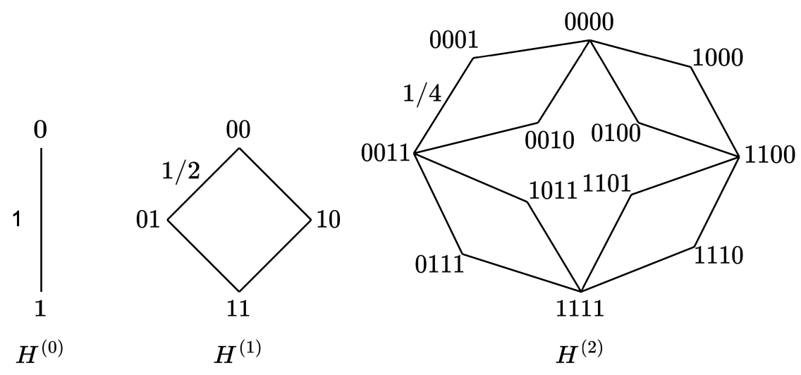
Figure 9: The recursive diamond graph in Hamming space.

The $n^{\text{th}}$ level of this recursive construction $H^{(n)}$ has $M=\frac{2}{3}\cdot 4^{n}+\frac{4}{3}$ many Hamming vectors. To obtain $H^{(n+1)}$ from $H^{(n)}$, any edge connecting two vectors at a (normalized) Hamming distance of $1/2^{n}$ is split up, and two new vectors that are at a distance of $1/2^{n+1}$ from each of the these are introduced. [CS02, Theorem 2.1] asserts that embedding these vectors into $\ell_{1}$ with $O(1)$ distortion requires $M^{\Omega(1)}$ dimensions.

We construct a Bayesian network that has the same distances as the diamond graph above. Refer to Figure 10.

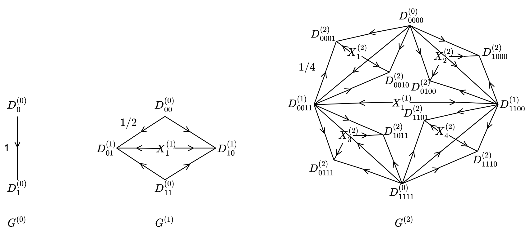
Figure 10: A Bayesian network based on the recursive diamond graph.

Each level $G^{(n)}$ of the instance consists of some $D$ nodes and some $X$ nodes. The $D$ nodes correspond to the points in Hamming space from Figure 9, while the $X$ nodes simulate 50-50 coin flips. The $(n+1)^{\text{th}}$ level $G^{(n+1)}$ of the instance is constructed from $G^{(n)}$ by splitting every edge connecting two $D^{(n)}$ nodes at a distance of $1/2^{n}$, introducing two new $D^{(n+1)}$ nodes and an $X^{(n+1)}$ node in the process. Table 1 summarizes the properties of this recursive construction:

Level	$G^{(0)}$	$G^{(1)}$	$G^{(2)}$	$G^{(3)}$	…	$G^{(n)}$
#splittable edges	1	4	16	64	…	$4^{n}$
#$D$ nodes	2	4	12	44	…	$\frac{2}{3}\cdot 4^{n}+\frac{4}{3}$
#$X$ nodes	0	1	5	21	…	$\frac{1}{3}\cdot 4^{n}-\frac{1}{3}$

Table 1: Properties of $G^{(n)}$.

To obtain a sample from the Bayesian network, we first independently sample a 50-50 coin flip for every $X$ node in the network. The $D$ nodes can then be sampled in a hierarchical manner. First, the $D$ nodes in the $0^{\text{th}}$ level are deterministically set: $D^{(0)}_{0\dots 0}=0$ and $D^{(0)}_{1\dots 1}=1$ with probability 1. Then, for $n=1,2,\dots$, we inductively realize $D^{(n)}$ nodes as follows: let $D^{(n)}_{x}$ and $D^{(n)}_{y}$ be nodes that arise from splitting an edge $(D^{(n-1)}_{u},D^{(n-1)}_{v})$ with node $X^{(n)}_{i}$, and let $x<y$ and $u<v$ lexicographically. Recall that $D^{(n-1)}_{u},D^{(n-1)}_{v}$ and $X^{(n)}_{i}$ have already been realized. Then,

$$D^{(n)}_{x}\leftarrow D^{(n-1)}_{u},D^{(n)}_{y}\leftarrow D^{(n-1)}_{v},\qquad\text{if }X^{(n)}_{i}=0$$

$$D^{(n)}_{x}\leftarrow D^{(n-1)}_{v},D^{(n)}_{y}\leftarrow D^{(n-1)}_{u},\qquad\text{if }X^{(n)}_{i}=1.$$

In other words, $X^{(n)}_{i}$ acts as a “switch” node. We can verify that the distances between the $D$ nodes mimic the distances between the corresponding Hamming vectors. Concretely,

$$\operatorname{{Pr}}[D^{(n)}_{x}\neq D^{(n)}_{y}]=\|x-y\|_{1}.$$

Furthermore, the marginal probability of a $D$ node being equal to 1 is exactly equal to the fraction of $1$’s in the Hamming vector representing it.

Observe that $G^{(n)}$ has $N<2M$ many $D$+$X$ nodes in total, where $M=\frac{2}{3}\cdot 4^{n}+\frac{4}{3}$ is the number of Hamming vectors in $H^{(n)}$ above. If we were able to embed the nodes of $G^{(n)}$ into $\ell_{1}$ with constant distortion in $N^{o(1)}=M^{o(1)}$ dimensions, we can use the embeddings of the $D$ nodes as the embeddings of the Hamming vectors in the lower bound instance from [CS02] (i.e., Figure 9 above), and this will give us an $M^{o(1)}$ dimensional embedding of the recursive diamond graph, which we know is not possible. Thus, any constant-distortion embedding of $G^{(n)}$—a Bayesian network on $N$ nodes—into $\ell_{1}$, necessarily requires $N^{\Omega(1)}$ many dimensions.

We will now argue that the undirected graph underlying $G^{(n)}$ for any $n\geq 1$ has treewidth equal to 3. We will slightly abuse notation and refer to the undirected graph underlying $G^{(n)}$ by $G^{(n)}$.

To see that the treewidth is at least 3, we note that the treewidth of a graph is at least the treewidth of any subgraph of the graph. For $n\geq 1$, observe that $G^{(n)}$ contains the subgraph underlying $G^{(1)}$, and we can verify, e.g., by brute-force, that this small subgraph has treewidth equal to 3.

We will now show that the treewidth of $G^{(n)}$ is at most 3. For this, we appeal to the definition of the treewidth based on elimination orderings of the nodes [PCdG⁺19, Definition 1]. This definition is especially well-suited in the context of inference via variable elimination in graphical models. An equivalent form of this definition is as follows: first, we specify an ordering over the nodes in the graph. Then, we eliminate nodes in the graph in this order. Whenever we eliminate a node, we add an edge (if there isn’t one already) between every pair of its neighbors that are still surviving. Before we eliminate a node, we record the count of nodes it is connected to. The maximum count that we see until we eliminate all nodes is the treewidth with respect to this ordering, and the smallest maximum count over all orderings is the graph’s treewidth.

Thus, to show that the treewidth of $G^{(n)}$ is at most 3, we only need to come up with an ordering that witnesses treewidth to be at most $3$. Given the hierarchical structure of $G^{(n)}$, this ordering is natural—we start eliminating nodes from the highest level to the lowest level. Concretely, we first eliminate all the $D^{(n)}$ nodes, in say lexicographical order. Then, we eliminate all the $X^{(n)}$ nodes (again, in say lexicographical order). We then eliminate all the $D^{(n-1)}$ nodes, followed by all the $X^{(n-1)}$ nodes, and so on, all the way until we empty the graph.

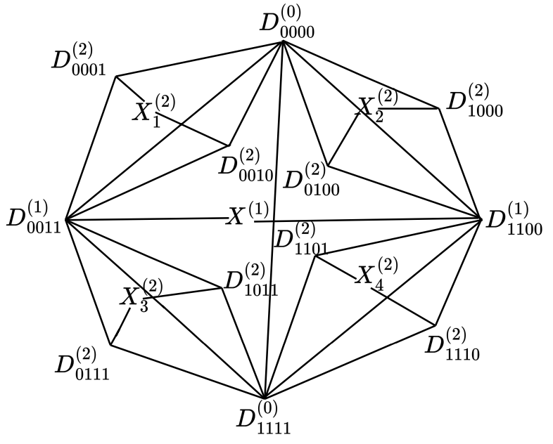
(a) $G^{(2)}$

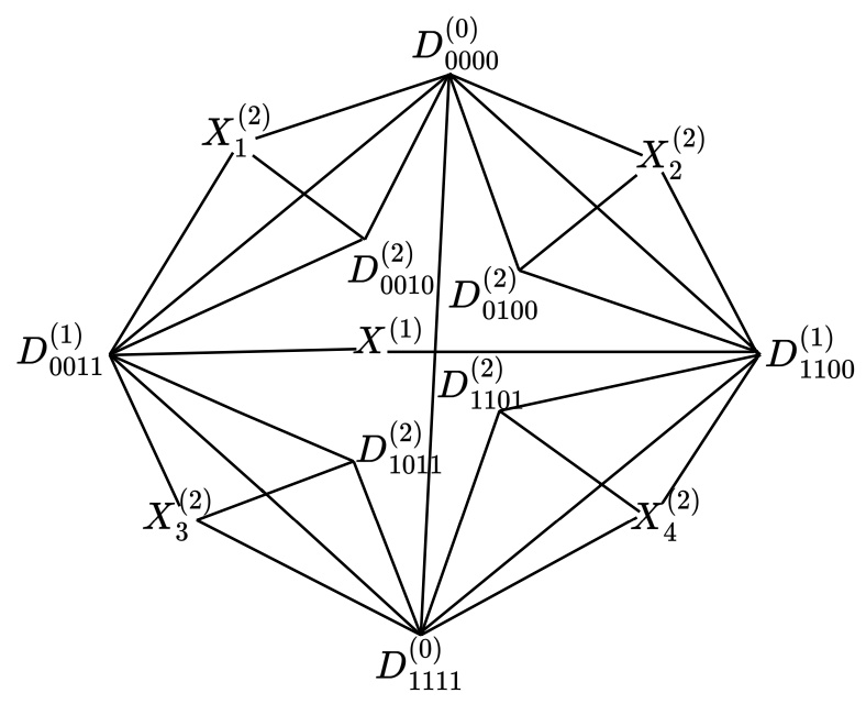
(b) Half the $D^{(2)}$ nodes eliminated.

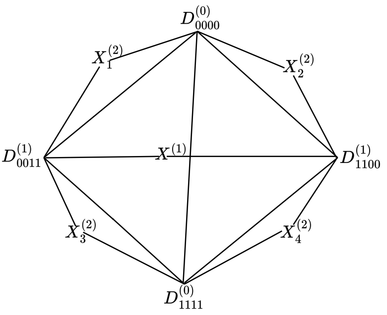
(c) All $D^{(2)}$ nodes eliminated.

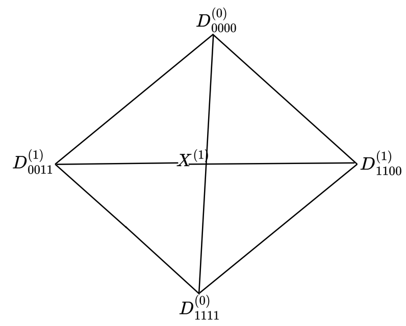
(d) $X^{(2)}$ nodes eliminated. This is $G^{(1)}$.

Figure 11: Level-wise elimination of nodes in $G^{(n)}$.

To see that the maximum degree of any node that is about to be eliminated is at most 3, consider what happens in the example in Figure 11, where we start with $G^{(2)}$. First, we eliminate $D^{(2)}$ nodes, followed by $X^{(2)}$ nodes. Observe that the degree of any $D^{(2)}$ node prior to elimination is exactly 3—this corresponds to the two $D^{(1)}$ nodes and $X^{(1)}$ node generating it. After we eliminate a $D^{(2)}$ node, we must introduce pairwise edges between its neighbors—since there is already an edge between its parent $D^{(1)}$ nodes, we only need to add edges between the $X^{(1)}$ and $D^{(1)}$ nodes. Next, when it comes to eliminating the $X^{(2)}$ nodes, observe that the degree of these nodes prior to elimination is exactly 2—this corresponds to the two $D^{(1)}$ nodes that it split. Finally, when we eliminate these nodes, we don’t need to introduce any new edges, because the $D^{(1)}$ nodes that they are adjacent to were already connected by an edge. More importantly, observe that after this round of eliminating $D^{(2)}$ and $X^{(2)}$ nodes, we end up exactly with the graph underlying $G^{(1)}$! Thus, the same argument carries forward. More generally, for any $n$, when we eliminate $D^{(n)}$ and $X^{(n)}$ nodes, we end up with the graph underlying $G^{(n-1)}$, and the maximum degree of any node prior to elimination is at most 3. Thus, this ordering witnesses that the treewidth of $G^{(n)}$ is at most 3, as required. ∎

Given that we have a (partial) positive answer for the treewidth-1 case, and that there isn’t hope for a general result in the treewidth-3 case, this leaves the treewidth-2 case wide open (in addition to the open treewidth-1 case mentioned in 1).

Open Problem 2.

Let $D$ be a joint distribution on $N$ binary random variables $X_{1},\dots,X_{N}$ given by a Bayesian network whose underlying undirected graph has treewidth 2. Consider the metric $d_{D}(X_{i},X_{j})=\operatorname{{Pr}}_{D}[X_{i}\neq X_{j}]$. Does this metric embed into $\ell_{1}$ with constant distortion and with $N^{o(1)}$ dimensions?

Finally, our lower bound for treewidth-3 is not an Ising model, so it remains open whether more general classes of Ising models permit low dimension embeddings. For example, it is simple to embed an Ising model whose underlying graph is a cycle.

Open Problem 3.

Let $D$ be a joint distribution on $N$ binary random variables $X_{1},\dots,X_{n}$ given by an Ising model. Consider the metric $d_{D}(X_{i},X_{j})=\operatorname{{Pr}}_{D}[X_{i}\neq X_{j}]$. For what classes of graphs (e.g. bounded treewidth, general graphs) does this metric embed into $\ell_{1}$ with constant distortion and with $N^{o(1)}$ dimensions?

Appendix A Lazy Snaking for Lipschitz Cap Line Metrics

We restate and prove Lemma 5.14: See 5.14

Proof.

The first part of the claim is straightforward, since snaking can only reduce distance between two nodes.
For the second part, we will instead show that $\operatorname{{\mathds{E}}}[|embedding(i)-embedding(j)|]\geq\Omega(1)\cdot d^{{M^{\prime}}}_{\mathrm{lipcap}}(x_{i},x_{j})$, where $M^{\prime}(t)=\frac{47}{7447}M(t)$. This is sufficient, because $d^{{M^{\prime}}}_{\mathrm{lipcap}}(x_{i},x_{j})\geq\frac{47}{7447}d^{{M}}_{\mathrm{lipcap}}(x_{i},x_{j})$. Fix some $i<j$. Before reaching $loc[i]$, let $t_{1}$ be the last time we were at the origin and decided to either rest/snake, such that $t_{1}\leq loc[i]$. Then, it must have been the case that either (i) we decided to snake at $t_{1}$, and returned back to the origin at a time $t_{2}>loc[i]$, or (ii) we decided to rest but there was not another decision before $t_{2}>loc[i]$. Namely, we have

$$\frac{M(t_{1})}{300}\leq t_{2}-t_{1}\leq\max\left(\frac{M(t_{1})}{300},\frac{2M(t_{1})}{100}\right)=\frac{M(t_{1})}{50}.$$ (74)

$$t_{2}>loc[i]\implies t_{1}+\frac{M(t_{1})}{50}>loc[i]\implies loc[i]-t_{1}<\frac{M(t_{1})}{50}.$$ (75)

From Lipschitzness, we have,

$$|M(loc[i])-M(t_{1}))|\leq|loc[i]-t_{1}|\leq|t_{2}-t_{1}|\leq\frac{M(t_{1})}{50}$$

$$\implies\qquad \frac{49}{50}M(t_{1})\leq M(loc[i])\leq\frac{51}{50}M(t_{1}).$$ (76)

Combining with Equation 75, we get

$$loc[i]-t_{1}<\frac{M(loc[i])}{49}.$$ (77)

Observe also that by Lipschitzness, for every $t\in[t_{1},t_{2}]$, we have

$$|M(loc[i])-M(t)|\leq|loc[i]-t|\leq|t_{2}-t_{1}|\leq\frac{M(t_{1})}{50}\leq\frac{M(loc[i])}{49}$$ (78)

$$\implies\qquad \frac{48M(loc[i])}{49}\leq M(t)\leq\frac{50M(loc[i])}{49}.$$ (79)

Let $E$ be the event that $snake[t_{1}]=0$ for some $t_{1}\in\left[loc[i]-\frac{M(loc[i])}{49},loc[i]\right]$, such that we are ready to flip a coin at $t_{1}$. Then, Equation 77 implies that $\operatorname{{Pr}}[E]=1$. Repeating the same argument as above, but from the perspective of $t_{1}$, we get that there also exists a $t_{0}\in\left[loc[i]-\frac{M(loc[i])}{49}-\frac{50}{49}\frac{M(loc[i])}{49},loc[i]-\left(\frac{50}{51}\right)^{2}\frac{M(loc[i])}{300}\right]$ such that with probability 1, $snake[t_{0}]=0$ and we about to flip at $t_{0}$. We note here that $t$ was initialized to $-2M(0)$ in Step 1 of Algorithm 2 precisely to ensure that such a $t_{0}$ always exists. Initializing in this manner ensures that there is always a distance of $\frac{M(loc[i])}{49}+\frac{50}{49}\frac{M(loc[i])}{49}$ before every $loc[i]$—if there wasn’t, Lipschitzness would be violated.

We will first do the analysis for the setting where $M(loc[i])\geq M(loc[j])$, so that $\max(M(loc[i]),M(loc[j]))$ $=M(loc[i])$. The analysis for $M(loc[i])<M(loc[j])$ is very similar, and is presented afterwards. We have three cases:

Case 1a: $0<|loc[i]-loc[j]|\leq\frac{47}{7447}M(loc[i]).$
Here, $d^{{M^{\prime}}}_{\mathrm{lipcap}}(x_{i},x_{j})=|loc[i]-loc[j]|$. First, we invoke Equation 77 and condition on arriving at $t_{1}\in\left[loc[i]-\frac{M(loc[i])}{49},loc[i]\right]$, where $snake[t_{1}]=0$ and we are about to flip a coin. Starting at $t_{1}$, observe that with at most $\frac{M(loc[i])}{49}\cdot\frac{49\cdot 300}{48M(loc[i])}=\Theta(1)$ “rest” flips, we get to a $t\in\left[loc[i]-\frac{50M(loc[i])}{49\cdot 300},loc[i]\right]$ such that $snake[t]=0$. This is because $t_{1}$ is at most $\frac{M(loc[i])}{49}$ away from $loc[i]$, and the each resting period is at least $\frac{48M(loc[i])}{49\cdot 300}$ and at most $\frac{50M(loc[i])}{49\cdot 300}$. Now, at $t$, we can flip a “snake”, for which the snaking width is at least $\frac{48M(loc[i])}{49\cdot 100}$. Observe that 1) $loc[i]$ is at most $\frac{50M(loc[i])}{49\cdot 300}$ from $t$, 2) $loc[j]$ is at most $\frac{47}{7447}M(loc[i])$ away from $loc[i]$ and 3) $\frac{50M(loc[i])}{49\cdot 300}+\frac{47}{7447}M(loc[i])\leq\frac{48M(loc[i])}{49\cdot 100}$. Together, this ensures that both $loc[i]$ and $loc[j]$ are encountered going forward from $t$ within one snaking width, i.e., $snake[loc[j]]-snake[loc[i]]=loc[j]-loc[i]=d^{{M^{\prime}}}_{\mathrm{lipcap}}(x_{i},x_{j})$.

Case 2a: $\frac{47}{7447}M(loc[i])<|loc[i]-loc[j]|\leq\frac{99}{2401}M(loc[i]).$
In this case, $d^{{M^{\prime}}}_{\mathrm{lipcap}}(x_{i},x_{j})=\frac{47}{7447}M(loc[i])$. Repeating the same reasoning as above, we start at $t_{1}$, and then get to a $t\in\left[loc[i]-\frac{50M(loc[i])}{49\cdot 300},loc[i]\right]$ such that $snake[t]=0$ with a constant number of “rest” flips. Now, we flip another “rest”, which ensures that $snake[loc[i]]=0$, and gets us to a $t\in\left[loc[i],loc[i]+\frac{50M(loc[i])}{49\cdot 300}\right]$. Note that since $|loc[i]-loc[j]|>\frac{47}{7447}M(loc[i])>\frac{50M(loc[i])}{49\cdot 300}$ we know $t<loc[j]$ and that there is still some distance left to get to $loc[j]$. Now, for any $t\in[loc[i],loc[j]]$, by Lipschitzness, we have

$$|M(t)-M(loc[i])|\leq|loc[i]-loc[j]|\leq\frac{99}{2401}M(loc[i]),$$

which means that $M(t)\in\left[\frac{2392}{2401}M(loc[i]),\frac{2500}{2401}M(loc[i])\right]$. Therefore, with at most $\frac{99M(loc[i])}{2401}\cdot\frac{2401\cdot 300}{2392M(loc[i])}=\Theta(1)$ “rest” flips, we get to a $t$ which is in $\left[loc[j]-\frac{50M(loc[i])}{49\cdot 300\cdot 2}-\frac{2500M(loc[i])}{2401\cdot 300},loc[j]-\frac{50M(loc[i])}{49\cdot 300\cdot 2}\right]$. Once here, we can flip a “snake”—noting that 1) the snaking width is at least $\frac{2392}{2401\cdot 100}M(loc[i])$ 2) the distance to $loc[j]$ is at most $\frac{50M(loc[i])}{49\cdot 300\cdot 2}+\frac{2500M(loc[i])}{2401\cdot 300}$ and 3) the quantity in 2) is smaller than the quantity in 1), we get that $snake[loc[j]]$ is at least $\frac{50M(loc[i])}{49\cdot 300\cdot 2}$, which is at least a constant fraction of $d^{{M^{\prime}}}_{\mathrm{lipcap}}(x_{i},x_{j})$.

Case 3a: $\frac{99}{2401}M(loc[i])<|loc[i]-loc[j]|.$
In this case, $d^{{M^{\prime}}}_{\mathrm{lipcap}}(x_{i},x_{j})=\frac{47}{7447}M(loc[i])$. We argued above that with probability 1, there exists a $t_{0}\in\left[loc[i]-\frac{M(t_{1})}{50}-\frac{M(t_{0})}{50},loc[i]-\frac{M(t_{0})}{300}\right]\in\left[loc[i]-\frac{99M(loc[i])}{2401},loc[i]-\left(\frac{50}{51}\right)^{2}\frac{M(loc[i])}{300}\right]$ such that $snake[t_{0}]=0$ and we are about to flip a coin. Observe that by Lipschitzness, for any $t\in[t_{0},loc[i]]$,

$$M(t)\in\left[\frac{2392}{2401}M(loc[i]),\frac{2500}{2401}M(loc[i])\right].$$

Therefore, with at most $\frac{99M(loc[i])}{2401}\cdot\frac{2401\cdot 300}{2392M(loc[i])}=\Theta(1)$ “rest” flips, we get to a $t$ which is in

$$\left[loc[i]-\left(\frac{50}{51}\right)^{2}\frac{M(loc[i])}{300}-\frac{2500M(loc[i])}{2401\cdot 300},loc[i]-\left(\frac{50}{51}\right)^{2}\frac{M(loc[i])}{300}\right].$$

Now, we may flip a “snake”—noting that 1) the snaking width is at least $\frac{2392M(loc[i])}{2401\cdot 100}$ and 2) the distance to $loc[i]$ is at least $\left(\frac{50}{51}\right)^{2}\frac{M(loc[i])}{300}$ and at most $\left(\frac{50}{51}\right)^{2}\frac{M(loc[i])}{300}+\frac{2500M(loc[i])}{2401\cdot 300}<\frac{2392M(loc[i])}{2401\cdot 100}$, we can conclude that by the time we get to $loc[i]$, $snake[loc[i]]$ will at least be $\left(\frac{50}{51}\right)^{2}\frac{M(loc[i])}{300}=\Omega(1)\cdot d^{{M^{\prime}}}_{\mathrm{lipcap}}(x_{i},x_{j})$. Next, we know that with probability 1, there exists a $t^{\prime}\in\left[loc[j]-\frac{M(loc[j])}{49},loc[j]\right]$ such that $snake[t^{\prime}]=0$ and we are about flip a coin. Further, this $t^{\prime}$ is larger than $loc[i]$, because $loc[j]-\frac{M(loc[j])}{49}$ needs to be larger than $loc[i]$ under the case we are studying. We catch hold of this $t^{\prime}$, and with a constant number of “rest” flips, we ensure that $snake[loc[j]]=0$. Thus, we obtain that $|snake[loc[i]]-snake[loc[j]]|\geq\Omega(1)\cdot d^{{M^{\prime}}}_{\mathrm{lipcap}}(x_{i},x_{j})$.

Now, we will do the analysis for when $M(loc[i])<M(loc[j])$, so that $\max(M(loc[i]),M(loc[j]))$ $=M(loc[j])$. Again, we have three cases:

Case 1b: $0<|loc[i]-loc[j]|\leq\frac{47}{7447}M(loc[j]).$
Here, $d^{{M^{\prime}}}_{\mathrm{lipcap}}(x_{i},x_{j})=|loc[i]-loc[j]|$. By Lipschitzness, we have $M(loc[i])\in\left[\frac{7400}{7447}M(loc[j]),\frac{7494}{7447}M(loc[j])\right]$. First, we condition on arriving at $t_{1}$, where $snake[t_{1}]=0$ and we are about to flip a coin. Starting at $t_{1}$, observe that with at most $\frac{M(loc[i])}{49}\cdot\frac{49\cdot 300}{48M(loc[i])}=\Theta(1)$ “rest” flips, we get to a $t\in\left[loc[i]-\frac{50M(loc[i])}{49\cdot 300},loc[i]\right]$ such that $snake[t]=0$ and we are about to flip a coin. Now, at $t$, we can flip a “snake”, for which the snaking width is at least $\frac{48M(loc[i])}{49\cdot 100}\geq\frac{7400\cdot 48M(loc[j])}{7447\cdot 49\cdot 100}$. Observe that 1) $loc[i]$ is at most $\frac{50M(loc[i])}{49\cdot 300}\leq\frac{7494\cdot 50M(loc[j])}{7447\cdot 49\cdot 300}$ from $t$, 2) $loc[j]$ is at most $\frac{47}{7447}M(loc[j])$ away from $loc[i]$ and 3) $\frac{7494\cdot 50M(loc[j])}{7447\cdot 49\cdot 300}+\frac{47}{7447}M(loc[j])\leq\frac{7400\cdot 48M(loc[j])}{7447\cdot 49\cdot 100}$. Together, this ensures that both $loc[i]$ and $loc[j]$ are encountered going forward from $t$ within one snaking width, i.e., $snake[loc[j]]-snake[loc[i]]=loc[j]-loc[i]=d^{{M^{\prime}}}_{\mathrm{lipcap}}(x_{i},x_{j})$.

Case 2b: $\frac{47}{7447}M(loc[j])<|loc[i]-loc[j]|\leq\frac{99}{2401}M(loc[j]).$
In this case, $d^{{M^{\prime}}}_{\mathrm{lipcap}}(x_{i},x_{j})=\frac{47}{7447}M(loc[j])$. Repeating the same reasoning as above, we start at $t_{1}$, and then get to a $t\in\left[loc[i]-\frac{50M(loc[i])}{49\cdot 300},loc[i]\right]$ such that $snake[t]=0$ with a constant number of “rest” flips. Now, we flip another “rest”, which ensures that $snake[loc[i]]=0$, and gets us to a $t\in\left[loc[i],loc[i]+\frac{50M(loc[i])}{49\cdot 300}\right]$. Since, $M[loc[i]]<M[loc[j]]$, $t\in\left[loc[i],loc[i]+\frac{50M(loc[j])}{49\cdot 300}\right]$. Note that since $|loc[i]-loc[j]|>\frac{47}{7447}M(loc[j])>\frac{50M(loc[j])}{49\cdot 300}$ we know $t<loc[j]$ and there is still some distance left to reach $loc[j]$. Now, for any $t\in[loc[i],loc[j]]$, by Lipschitzness, we have

$$|M(t)-M(loc[j])|\leq|loc[i]-loc[j]|\leq\frac{99}{2401}M(loc[j]),$$

which means that $M(t)\in\left[\frac{2392}{2401}M(loc[j]),\frac{2500}{2401}M(loc[j])\right]$. Therefore, with at most $\frac{99M(loc[j])}{2401}\cdot\frac{2401\cdot 300}{2392M(loc[j])}=\Theta(1)$ “rest” flips, we get to a $t$ which is in $\left[loc[j]-\frac{50M(loc[j])}{49\cdot 300\cdot 2}-\frac{2500M(loc[j])}{2401\cdot 300},loc[j]-\frac{50M(loc[j])}{49\cdot 300\cdot 2}\right]$. Once here, we can flip a “snake”—noting that 1) the snaking width is at least $\frac{2392}{2401\cdot 100}M(loc[j])$ and 2) the distance to $loc[j]$ is at most $\frac{50M(loc[j])}{49\cdot 300\cdot 2}+\frac{2500M(loc[j])}{2401\cdot 300}$, and 3) the quantity in 2) is smaller than the quantity in 1), we get that $snake[loc[j]]$ is at least $\frac{50M(loc[j])}{49\cdot 300\cdot 2}$, which is at least a constant fraction of $d^{{M^{\prime}}}_{\mathrm{lipcap}}(x_{i},x_{j})$.

Case 3b: $\frac{99}{2401}M(loc[j])<|loc[i]-loc[j]|.$
In this case, $d^{{M^{\prime}}}_{\mathrm{lipcap}}(x_{i},x_{j})=\frac{47}{7447}M(loc[j])$. We know that with probability 1, there exists a

$$t^{\prime}\in\left[loc[i]-\frac{M(loc[i])}{49},loc[i]\right]$$

such that $snake[t^{\prime}]=0$ and we are about flip a coin. We catch hold of $t^{\prime}$, and with a constant number of “rest” flips, we ensure that $snake[loc[i]]=0$. Next, we argued above that with probability 1, there exists a $t_{0}\in\left[loc[j]-\frac{M(t_{0})}{50}-\frac{M(t_{1})}{50}\right]\in\left[loc[j]-\frac{99M(loc[j])}{2401},loc[j]-\left(\frac{50}{51}\right)^{2}\frac{M(loc[j])}{300}\right]$ such that $snake[t_{0}]=0$ and we are about to flip a coin. Observe that by Lipschitzness, for any $t\in[t_{0},loc[j]]$, $M(t_{0})\in\left[\frac{2392}{2401}M(loc[j]),\frac{2500}{2401}M(loc[j])\right]$. Therefore, with at most $\frac{99M(loc[j])}{2401}\cdot\frac{2401\cdot 300}{2392M(loc[j])}=\Theta(1)$ “rest” flips, we get to a $t$ which is in $\left[loc[j]-\left(\frac{50}{51}\right)^{2}\frac{M(loc[j])}{300}-\frac{2500M(loc[j])}{2401\cdot 300},loc[j]-\left(\frac{50}{51}\right)^{2}\frac{M(loc[j])}{300}\right]$. Now, we may flip a “snake”—noting that 1) the snaking width is at least $\frac{2392M(loc[j])}{2401\cdot 100}$ and 2) the distance to $loc[j]$ is at least $\left(\frac{50}{51}\right)^{2}\frac{M(loc[j])}{300}$ and at most $\left(\frac{50}{51}\right)^{2}\frac{M(loc[j])}{300}+\frac{2500M(loc[j])}{2401\cdot 300}<\frac{2392M(loc[j])}{2401\cdot 100}$, we can conclude that by the time we get to $loc[j]$, $snake[loc[j]]$ will at least be $\left(\frac{50}{51}\right)^{2}\frac{M(loc[j])}{300}=\Omega(1)\cdot d^{{M^{\prime}}}_{\mathrm{lipcap}}(x_{i},x_{j})$.

Finally, note that in every case, we showed that, conditioned on the outcomes of at most a constant number of coin flips, $|snake[loc[i]]-snake[loc[j]]|=|embedding[i]-embedding[j]|\geq\Omega(1)\cdot d^{{M^{\prime}}}_{\mathrm{lipcap}}(x_{i},x_{j})$. This immediately gives that $\operatorname{{\mathds{E}}}[|embedding[i]-embedding[j]|]\geq\Omega(1)\cdot d^{{M^{\prime}}}_{\mathrm{lipcap}}(x_{i},x_{j})$, completing the proof. ∎

Appendix B Proofs for General Capped $\ell_{1}$ Metrics

B.1 Coordinate-wise Embeddings are Good

In this section, we will essentially reuse the analysis of the build-clean procedure from Section 5.3.2 in order to prove Lemma 6.1. We restate the lemma here for convenience. See 6.1

Proof.

The proof is constructive. Without loss of generality, consider say the first coordinate of each of the $n$ points. We overload notation here and identify this coordinate of each point with $x_{1},\dots,x_{n}$. If we map these coordinates to the line, we obtain a line graph metric. Our goal is to embed this line metric with a fixed cap $M$—we will do so using the build-clean framework from Section 5.3.2. We will root the line at the leftmost point on the line (say this is $r$). For technical reasons again, we add an additional node $r_{0}$ at a distance $2M$ to the left of $r$. We will split up the line into edges of length $\frac{M}{100d}$—these edges correspond to the “shortened” caterpillar edges from the tree decomposition in Section 5.3.2. We group edges into build and clean stages. As before, each edge $e$ has auxiliary information $a(e)$ associated with it which determines whether it is processed in the build/clean stage. We set $L_{\textrm{build}}=4d$ and $L_{\textrm{clean}}=9d$. The auxiliary information for the leftmost/first edge is chosen uniformly at random from $\{0,\dots,L_{\textrm{build}}+L_{\textrm{clean}}-1\}$. Thereafter, for every edge $e$, $a(e)=a(par(e))+1\mod(L_{\textrm{build}}+L_{\textrm{clean}})$, where $par(e)$ is simply the adjacent edge to the left of $e$. If $a(e)\in\{0,\dots,L_{\textrm{build}}-1\}$, $e$ is processed in the build stage, else it is processed in the clean stage. After processing all the edges, all the points on the line will be mapped to an embedding of size $|H|=8d$. We construct this $|H|$-sized embedding for every location on the line metric in the same way as described in Section 5.3.2 for Lipschitz-cap trees. In the language of the analysis there, let $embedding[1],\dots,embedding[n]$ denote the embeddings thus obtained (these correspond to the vectors $v^{(1)}_{1},\dots,v^{(1)}_{n}$ in the language of Lemma 6.1). To avoid simply rewriting the entire analysis from Section 5.3.2, we will walk through the claims therein in a stepwise manner, and only specify the parts relevant to the special case we are in, i.e., a line graph with a fixed cap.

Since the cap at every location is equal to $M$, we do not need to relate the caps of points on nearby edges, as we did in 5.15 and 5.16.

Next, 5.17 holds too—at any location $x$ immediately after processing an entire clean stage, all the coordinates of $embedding[x]$ are identically 0. While the same proof in 4.2 works, we can also see this more directly here. The build stage, by virtue of processing only at most $4d$ edges, fills in only at most $4d$ coordinates to a value $\frac{M}{100d}$, while a complete clean stage comprises of $9d$ edges of length $\frac{M}{100d}$, and hence definitely zeros out all the nonzero coordinates.

Because of complete cleaning, the proof in 5.18 would similarly give us that for any location $x$, $\|embedding[x]\|_{1}\leq\frac{M}{2}$ (actually, we would obtain a stronger bound of $\frac{M}{25}$, but the weaker bound suffices).

At this point, we have already proved part (1) of Lemma 6.1. Because of the way the build-clean procedure works, the embeddings as we move continuously along the line are coordinate-wise Lipschitz, and only ever capture distance in one coordinate along adjacent locations. This already gives us that $\|embedding[i]-embedding[j]\|_{1}\leq|x_{i}-x_{j}|$. From the norm bound on the embedding, we also have that

$$\|embedding[i]-embedding[j]\|_{1}\leq\|embedding[i]\|_{1}+\|embedding[j]\|_{1}\leq M.$$

Hence, we have that $\|embedding[i]-embedding[j]\|_{1}\leq\min(|x_{i}-x_{j}|,M)$.

Next, we turn our attention towards proving part (2) of the lemma. Consider the guarantee given by 5.19. Let $x_{i}$ be to the left of $x_{j}$ without loss of generality. Then, the LCA of $x_{i}$ and $x_{j}$ on the line would simply be $x_{i}$. The same proof, with “$\log(n)$” replaced with “$d$” would yield that

$$\operatorname{{\mathds{E}}}\left[\|embedding[x_{i}]-embedding[x_{j}]\|_{1}\right]\geq\Omega(1)\cdot\min(|x_{i}-x_{j}|,M),$$ (80)

and this is precisely what we wanted to prove for the purposes of part(2) in Lemma 6.1. ∎

B.2 Concatenations of Coordinate-wise Embeddings are Good

First, we state a reverse application of Markov’s inequality:

Proposition B.1 (Reverse Markov).

Let $F$ be a random variable such that $F\in[0,M]$ with probability 1, and $\operatorname{{\mathds{E}}}[F]\geq c_{1}M$, for $c_{1}\leq 1$. Then, for any $C_{2}\geq 1$,

$$\operatorname{{Pr}}\left[F\geq\frac{c_{1}}{C_{2}}\cdot M\right]\geq 1-\frac{1-c_{1}}{1-\frac{c_{1}}{C_{2}}}.$$

Proof.

Define $G=M-F$, so that $G\in[0,M]$. Then $\operatorname{{\mathds{E}}}[G]=M-\operatorname{{\mathds{E}}}[F]\leq M-c_{1}M$. Applying Markov’s inequality,

$$\operatorname{{Pr}}\left[F<\frac{c_{1}}{C_{2}}\cdot M\right]=\operatorname{{Pr}}\left[G>\left(1-\frac{c_{1}}{C_{2}}\right)\cdot M\right]\leq\frac{1-c_{1}}{1-\frac{c_{1}}{C_{2}}}$$

$$\implies\qquad \operatorname{{Pr}}\left[F\geq\frac{c_{1}}{C_{2}}\cdot M\right]\geq 1-\frac{1-c_{1}}{1-\frac{c_{1}}{C_{2}}}.$$

∎

We can now use Proposition B.1 to prove the following general result which we can directly use to prove that the $z_{i}$ vectors constructed in Section 6 capture the capped distance well.

Lemma B.2.

Suppose $R_{1},\dots,R_{d}$ are independent random variables such that each $R_{i}\in[0,M]$ with probability 1, and $\operatorname{{\mathds{E}}}[\sum_{i=1}^{d}R_{i}]\geq c\cdot M$ for a constant $c\leq 1$. Then,

$$\operatorname{{Pr}}\left[\sum_{i=1}^{d}R_{i}\geq\frac{c^{2}}{100}\cdot M\right]\geq\Omega(1).$$

Proof.

Assume for the sake of contradiction that

$$\operatorname{{Pr}}\left[\sum_{i=1}^{d}R_{i}\geq\frac{c^{2}}{100}\cdot M\right]<\min\left(\frac{1}{100},1-\frac{1-\left(\frac{99c}{100}\right)^{2}}{1-\frac{c^{2}}{100}}\right).$$

In particular, since the $R_{i}$s are non-negative, this implies that

$$\operatorname{{Pr}}\left[\sum_{i=1}^{j}R_{i}\geq\frac{c^{2}}{100}\cdot M\right]<\min\left(\frac{1}{100},1-\frac{1-\left(\frac{99c}{100}\right)^{2}}{1-\frac{c^{2}}{100}}\right)\quad\text{for all $j\in\{1,\dots,d\}$}.$$ (81)

We will reason about the random variable

$$\min\left(\sum_{i=1}^{d}R_{i},cM\right)=\sum_{i=1}^{d}\min\left[R_{i},\max\left(0,cM-\sum_{j=1}^{i-1}R_{j}\right)\right].$$

Let $A_{i}$ be the event that $\sum_{j=1}^{i}R_{j}<\frac{c}{100}\cdot M$ and $B_{i}$ be the event that $\sum_{j=1}^{i}R_{j}<\frac{c^{2}}{100}\cdot M$. Further, let $\mathds{1}[A_{i}]$ and $\mathds{1}[B_{i}]$ be their indicators. Note that $\operatorname{{Pr}}[B_{i}]\leq\operatorname{{Pr}}[A_{i}]$, since $c\leq 1$. Then, observe that

$$\min\left[R_{i},\max\left(0,cM-\sum_{j=1}^{i-1}R_{j}\right)\right] \geq\mathds{1}[A_{i-1}]\cdot\min\left(R_{i},\frac{99c}{100}\cdot M\right)$$

$$\geq\mathds{1}[A_{i-1}]\cdot\frac{99c}{100}\cdot R_{i}.$$

Here, the last inequality follows because $\frac{99c}{100}\cdot R_{i}\leq\frac{99c}{100}\cdot M$ as well as $\frac{99c}{100}\cdot R_{i}\leq R_{i}$, since $c\leq 1$. Thus, we obtain that

$$\operatorname{{\mathds{E}}}\left[\min\left(\sum_{i=1}^{d}R_{i},cM\right)\right] =\operatorname{{\mathds{E}}}\left[\sum_{i=1}^{d}\min\left[R_{i},\max\left(0,cM-\sum_{j=1}^{i-1}R_{j}\right)\right]\right]$$

$$\geq\operatorname{{\mathds{E}}}\left[\sum_{i=1}^{d}\mathds{1}[A_{i-1}]\cdot\frac{99c}{100}\cdot R_{i}\right]$$

$$=\sum_{i=1}^{d}\operatorname{{\mathds{E}}}\left[\mathds{1}[A_{i-1}]\cdot\frac{99c}{100}\cdot R_{i}\right]\qquad(\text{linearity of expectation})$$

$$=\frac{99c}{100}\cdot\sum_{i=1}^{d}\operatorname{{\mathds{E}}}\left[\mathds{1}[A_{i-1}]\right]\cdot\operatorname{{\mathds{E}}}\left[R_{i}\right]\qquad\text{(independence of $R_{i}$s)}$$

$$=\frac{99c}{100}\cdot\sum_{i=1}^{d}\operatorname{{Pr}}\left[A_{i-1}\right]\cdot\operatorname{{\mathds{E}}}\left[R_{i}\right]$$

$$\geq\frac{99c}{100}\cdot\sum_{i=1}^{d}\operatorname{{Pr}}\left[B_{i-1}\right]\cdot\operatorname{{\mathds{E}}}\left[R_{i}\right]\qquad\left(\text{since $\operatorname{{Pr}}[B_{i-1}]\leq\operatorname{{Pr}}[A_{i-1}]$}\right)$$

$$\geq\frac{99c}{100}\cdot\frac{99}{100}\cdot\sum_{i=1}^{d}\operatorname{{\mathds{E}}}\left[R_{i}\right]\qquad\text{(\lx@cref{creftypecap~refnum}{eqn:reverse-markovish-contradiction})}$$

$$\geq\left(\frac{99c}{100}\right)^{2}M.$$

Now, we invoke Proposition B.1 with $F=\min\left(\sum_{i=1}^{d}R_{i},cM\right)$. Note that $F\in[0,M]$ with probability 1, and $\operatorname{{\mathds{E}}}[F]\geq\left(\frac{99c}{100}\right)^{2}\cdot M$ — thus, for $C_{2}=100\cdot\left(\frac{99}{100}\right)^{2}$, we get

$$\operatorname{{Pr}}\left[\min\left(\sum_{i=1}^{d}R_{i},cM\right)\geq\frac{c^{2}}{100}\cdot M\right] \geq 1-\frac{1-\left(\frac{99c}{100}\right)^{2}}{1-\frac{c^{2}}{100}}.$$

Notice that we have ended up showing

$$\operatorname{{Pr}}\left[\sum_{i=1}^{d}R_{i}\geq\frac{c^{2}}{100}\cdot M\right]\geq\operatorname{{Pr}}\left[\min\left(\sum_{i=1}^{d}R_{i},cM\right)\geq\frac{c^{2}}{100}\cdot M\right] \geq 1-\frac{1-\left(\frac{99c}{100}\right)^{2}}{1-\frac{c^{2}}{100}},$$

which contradicts Equation 81. Hence, it must be true that

$$\operatorname{{Pr}}\left[\sum_{i=1}^{d}R_{i}\geq\frac{c^{2}}{100}\cdot M\right]\geq\min\left(\frac{1}{100},1-\frac{1-\left(\frac{99c}{100}\right)^{2}}{1-\frac{c^{2}}{100}}\right)=\Omega(1).$$

∎

We are now ready to prove Lemma 6.2, which we resatate here for convenience. See 6.2

Proof.

Recall that $z_{i}$ is the concatenation of independently constructed vectors $v^{(q)}_{i}$ for $q\in\{1,\dots,d\}$. Let $R_{q}$ be the random variable $\|v^{q}_{i}-v^{(q)}_{j}\|_{1}$. Observe that the $R_{q}$’s are independent of each other, and that $\|z_{i}-z_{j}\|_{1}=\sum_{q=1}^{d}R_{q}$.
Case 1: $\|x_{i}-x_{j}\|_{1}\leq M.$
In this case, $d^{{M}}_{\mathrm{cap}}(x_{i},x_{j})=\|x_{i}-x_{j}\|_{1}$. Furthermore, for every $q$, $|x_{i}[q]-x_{j}[q]|\leq\|x_{i}-x_{j}\|_{1}$. From part (1) of Lemma 6.1, this means that for every $q$, $R_{q}=\|v^{q}_{i}-v^{(q)}_{j}\|_{1}\in[0,\|x_{i}-x_{j}\|_{1}]$ with probability 1. Furthermore, from part (2) of Lemma 6.1, $\operatorname{{\mathds{E}}}[R_{q}]\geq\Omega(1)\cdot|x_{i}[q]-x_{j}[q]|$. Thus,

$$\operatorname{{\mathds{E}}}\left[\sum_{q=1}^{d}R_{q}\right]\geq\Omega(1)\cdot\sum_{q=1}^{d}|x_{i}[q]-x_{j}[q]|=\Omega(1)\cdot\|x_{i}-x_{j}\|_{1}.$$

Instantiating Lemma B.2 with these $R_{q}$ variables, we get

$$\operatorname{{Pr}}\left[\sum_{q=1}^{d}R_{q}\geq\Omega(1)\cdot\|x_{i}-x_{j}\|_{1}\right]\geq\Omega(1)$$

$$\implies\qquad \operatorname{{Pr}}\left[\|z_{i}-z_{j}\|_{1}\geq\Omega(1)\cdot\|x_{i}-x_{j}\|_{1}\right]\geq\Omega(1).$$

Case 2: $\|x_{i}-x_{j}\|_{1}>M.$
In this case, $d^{{M}}_{\mathrm{cap}}(x_{i},x_{j})=M$. Observe first that for any $q\in\{1,\dots,d\}$, by part 1 of Lemma 6.1, $R_{q}\in[0,M]$ with probability 1. Next, observe also that $\operatorname{{\mathds{E}}}\left[\sum_{q=1}^{d}R_{q}\right]\geq\Omega(1)\cdot M$. To see this, consider two cases. In one case, there exists a coordinate $q$ such that $|x_{i}[q]-x_{j}[q]|>M$. In this case, part (2) of Lemma 6.1 already promises us that for this $q$, $\operatorname{{\mathds{E}}}[R_{q}]\geq\Omega(1)\cdot M$, and since the $R_{q}$’s are non-negative, we have the same lower bound on $\operatorname{{\mathds{E}}}\left[\sum_{q=1}^{d}R_{q}\right]$. In the remaining case, $|x_{i}[q]-x_{j}[q]|\leq M$ for all $q$. In this case, we can still apply part (2) of Lemma 6.1, to say that

$$\operatorname{{\mathds{E}}}\left[\sum_{q=1}^{d}R_{q}\right] =\sum_{q=1}^{d}\operatorname{{\mathds{E}}}\left[R_{q}\right]$$

$$\geq\sum_{q=1}^{d}\Omega(1)\cdot|x_{i}[q]-x_{j}[q]|$$

$$=\Omega(1)\cdot\|x_{i}-x_{j}\|_{1}$$

$$\geq\Omega(1)\cdot M,$$

where the last inequality follows because $\|x_{i}-x_{j}\|_{1}>M$ in the present case. Thus, we have shown that every $R_{q}$ is in $[0,M]$, and $\operatorname{{\mathds{E}}}\left[\sum_{q=1}^{d}R_{q}\right]\geq\Omega(1)\cdot M$. Instantiating Lemma B.2 gives

$$\operatorname{{Pr}}\left[\sum_{q=1}^{d}R_{q}\geq\Omega(1)\cdot M\right]\geq\Omega(1)$$

$$\implies\qquad \operatorname{{Pr}}\left[\|z_{i}-z_{j}\|_{1}\geq\Omega(1)\cdot M\right]\geq\Omega(1).$$

∎

References

- [ACNN11] Alexandr Andoni, Moses S Charikar, Ofer Neiman, and Huy L Nguyen. Near linear lower bound for dimension reduction in . In 2011 IEEE 52nd Annual Symposium on Foundations of Computer Science, pages 315--323. IEEE, 2011.
- [AKM+16] Amirali Abdullah, Ravi Kumar, Andrew McGregor, Sergei Vassilvitskii, and Suresh Venkatasubramanian. Sketching, embedding and dimensionality reduction in information theoretic spaces. In Artificial Intelligence and Statistics, pages 948--956. PMLR, 2016.
- [AORP10] Gonzalo R Arce, Daniel Otero, Ana B Ramirez, and Jose-Luis Paredes. Reconstruction of sparse signals from dimensionality-reduced cauchy random-projections. In 2010 IEEE International Conference on Acoustics, Speech and Signal Processing, pages 4014--4017. IEEE, 2010.
- [B+10] Christopher JC Burges et al. Dimension reduction: A guided tour. Foundations and Trends® in Machine Learning, 2(4):275--365, 2010.
- [BABK22] Enric Boix-Adsera, Guy Bresler, and Frederic Koehler. Chow-liu++: Optimal prediction-centric learning of tree ising models. In 2021 IEEE 62nd Annual Symposium on Foundations of Computer Science (FOCS), pages 417--426. IEEE, 2022.
- [BC05] Bo Brinkman and Moses Charikar. On the impossibility of dimension reduction in l1. Journal of the ACM (JACM), 52(5):766--788, 2005.
- [BFN19] Yair Bartal, Nova Fandina, and Ofer Neiman. Dimensionality reduction: theoretical perspective on practical measures. Advances in Neural Information Processing Systems, 32, 2019.
- [BGI+08] Radu Berinde, Anna C Gilbert, Piotr Indyk, Howard Karloff, and Martin J Strauss. Combining geometry and combinatorics: A unified approach to sparse signal recovery. In 2008 46th Annual Allerton Conference on Communication, Control, and Computing, pages 798--805. IEEE, 2008.
- [BGN15] Yair Bartal, Lee-Ad Gottlieb, and Ofer Neiman. On the impossibility of dimension reduction for doubling subsets of . SIAM Journal on Discrete Mathematics, 29(3):1207--1222, 2015.
- [BGPV21] Arnab Bhattacharyya, Sutanu Gayen, Eric Price, and NV Vinodchandran. Near-optimal learning of tree-structured distributions by chow-liu. In Proceedings of the 53rd annual acm SIGACT symposium on theory of computing, pages 147--160, 2021.
- [BK20] Guy Bresler and Mina Karzand. Learning a tree-structured ising model in order to make predictions. 2020.
- [BKR23] Zsolt Bartha, Júlia Komjáthy, and Järvi Raes. Sharp bound on the truncated metric dimension of trees. Discrete Mathematics, 346(8):113410, 2023.
- [BRV16] Alan F Beardon and Juan Alberto Rodríguez-Velázquez. On the k-metric dimension of metric spaces. arXiv preprint arXiv:1603.04049, 2016.
- [BSS21] Florent Baudier, Krzysztof Swieçicki, and Andrew Swift. No dimension reduction for doubling subsets of when revisited. Journal of Mathematical Analysis and Applications, 504(2):125407, 2021.
- [BVZ98] Yuri Boykov, Olga Veksler, and Ramin Zabih. Markov random fields with efficient approximations. In Proceedings. 1998 IEEE Computer Society Conference on Computer Vision and Pattern Recognition (Cat. No. 98CB36231), pages 648--655. IEEE, 1998.
- [CG15] John P Cunningham and Zoubin Ghahramani. Linear dimensionality reduction: Survey, insights, and generalizations. The Journal of Machine Learning Research, 16(1):2859--2900, 2015.
- [CGN+06] Chandra Chekuri, Anupam Gupta, Ilan Newman, Yuri Rabinovich, and Alistair Sinclair. Embedding -outerplanar graphs into . SIAM Journal on Discrete Mathematics, 20(1):119--136, 2006.
- [CGV16] Ferdinando Cicalese, Luisa Gargano, and Ugo Vaccaro. Approximating probability distributions with short vectors, via information theoretic distance measures. In 2016 IEEE International Symposium on Information Theory (ISIT), pages 1138--1142. IEEE, 2016.
- [CKNZ04] Chandra Chekuri, Sanjeev Khanna, Joseph Naor, and Leonid Zosin. A linear programming formulation and approximation algorithms for the metric labeling problem. SIAM Journal on Discrete Mathematics, 18(3):608--625, 2004.
- [CL68] CKCN Chow and Cong Liu. Approximating discrete probability distributions with dependence trees. IEEE transactions on Information Theory, 14(3):462--467, 1968.
- [CS02] Moses Charikar and Amit Sahai. Dimension reduction in the norm. In The 43rd Annual IEEE Symposium on Foundations of Computer Science, 2002. Proceedings., pages 551--560. IEEE, 2002.
- [CV22] Sourav Chatterjee and Mathukumalli Vidyasagar. Estimating large causal polytree skeletons from small samples. arXiv preprint arXiv:2209.07028, 2022.
- [CYBC23] Davin Choo, Joy Qiping Yang, Arnab Bhattacharyya, and Clément L Canonne. Learning bounded-degree polytrees with known skeleton. arXiv preprint arXiv:2310.06333, 2023.
- [Das13] Sanjoy Dasgupta. Learning polytrees. arXiv preprint arXiv:1301.6688, 2013.
- [DHK+21] Erik Demaine, Adam Hesterberg, Frederic Koehler, Jayson Lynch, and John Urschel. Multidimensional scaling: Approximation and complexity. In International Conference on Machine Learning, pages 2568--2578. PMLR, 2021.
- [DP21] Constantinos Daskalakis and Qinxuan Pan. Sample-optimal and efficient learning of tree ising models. In Proceedings of the 53rd Annual ACM SIGACT Symposium on Theory of Computing, pages 133--146, 2021.
- [EMP19] Ioannis Z Emiris, Vasilis Margonis, and Ioannis Psarros. Near neighbor preserving dimension reduction for doubling subsets of . arXiv preprint arXiv:1902.08815, 2019.
- [Fil20] Arnold Filtser. A face cover perspective to embeddings of planar graphs. In Proceedings of the Fourteenth Annual ACM-SIAM Symposium on Discrete Algorithms, pages 1945--1954. SIAM, 2020.
- [GKL03] Anupam Gupta, Robert Krauthgamer, and James R Lee. Bounded geometries, fractals, and low-distortion embeddings. In 44th Annual IEEE Symposium on Foundations of Computer Science, 2003. Proceedings., pages 534--543. IEEE, 2003.
- [GNRS04] Anupam Gupta, Ilan Newman, Yuri Rabinovich, and Alistair Sinclair. Cuts, trees and -embeddings of graphs. Combinatorica, 24(2):233--269, 2004.
- [GT00] Anupam Gupta and Éva Tardos. A constant factor approximation algorithm for a class of classification problems. In Proceedings of the thirty-second annual ACM symposium on Theory of computing, pages 652--658, 2000.
- [GY23] Paul Gutkovich and Zi Song Yeoh. Computing truncated metric dimension of trees. arXiv preprint arXiv:2302.05960, 2023.
- [IG98] Hiroshi Ishikawa and Davi Geiger. Segmentation by grouping junctions. In Proceedings. 1998 IEEE Computer Society Conference on Computer Vision and Pattern Recognition (Cat. No. 98CB36231), pages 125--131. IEEE, 1998.
- [IN07] Piotr Indyk and Assaf Naor. Nearest-neighbor-preserving embeddings. ACM Transactions on Algorithms (TALG), 3(3):31--es, 2007.
- [Jac17] Laurent Jacques. Small width, low distortions: quantized random embeddings of low-complexity sets. IEEE Transactions on information theory, 63(9):5477--5495, 2017.
- [JO12] Mohsen Jannesari and Behnaz Omoomi. The metric dimension of the lexicographic product of graphs. Discrete mathematics, 312(22):3349--3356, 2012.
- [KD16] M Kumar and Puneet Dokania. Rounding-based moves for semi-metric labeling. Journal of Machine Learning Research, 2016.
- [KDDC23] Vardis Kandiros, Constantinos Daskalakis, Yuval Dagan, and Davin Choo. Learning and testing latent-tree ising models efficiently. In Gergely Neu and Lorenzo Rosasco, editors, Proceedings of Thirty Sixth Conference on Learning Theory, volume 195 of Proceedings of Machine Learning Research, pages 1666--1729. PMLR, 12--15 Jul 2023.
- [KKMR06] Howard Karloff, Subhash Khot, Aranyak Mehta, and Yuval Rabani. On earthmover distance, metric labeling, and 0-extension. In Proceedings of the thirty-eighth annual ACM symposium on Theory of computing, pages 547--556, 2006.
- [KLR19] Robert Krauthgamer, James R Lee, and Havana Rika. Flow-cut gaps and face covers in planar graphs. In Proceedings of the Thirtieth Annual ACM-SIAM Symposium on Discrete Algorithms, pages 525--534. SIAM, 2019.
- [Kum14] M Pawan Kumar. Rounding-based moves for metric labeling. Advances in Neural Information Processing Systems, 27, 2014.
- [Kum22] Nikhil Kumar. An approximate generalization of the okamura-seymour theorem. In 2022 IEEE 63rd Annual Symposium on Foundations of Computer Science (FOCS), pages 1093--1101. IEEE, 2022.
- [KVT11] M Pawan Kumar, Olga Veksler, and Philip HS Torr. Improved moves for truncated convex models. The Journal of Machine Learning Research, 12:31--67, 2011.
- [KW16] Felix Krahmer and Rachel Ward. A unified framework for linear dimensionality reduction in l1. Results in Mathematics, 70:209--231, 2016.
- [LdMM13] James R Lee, Arnaud de Mesmay, and Mohammad Moharrami. Dimension reduction for finite trees in . Discrete & Computational Geometry, 50:977--1032, 2013.
- [LDRW18] Enrico Le Donne, Tapio Rajala, and Erik Walsberg. Isometric embeddings of snowflakes into finite-dimensional banach spaces. Proceedings of the American Mathematical Society, 146(2):685--693, 2018.
- [LM13] James R Lee and Mohammad Moharrami. A lower bound on dimension reduction for trees in . arXiv preprint arXiv:1302.6542, 2013.
- [LN04] James R Lee and Assaf Naor. Embedding the diamond graph in and dimension reduction in . Geometric & Functional Analysis GAFA, 14(4):745--747, 2004.
- [LN14] Vincent Lafforgue and Assaf Naor. A doubling subset of for that is inherently infinite dimensional. Geometriae Dedicata, 172:387--398, 2014.
- [Lot19] Martin Lotz. Persistent homology for low-complexity models. Proceedings of the Royal Society A, 475(2230):20190081, 2019.
- [LP01] Urs Lang and Conrad Plaut. Bilipschitz embeddings of metric spaces into space forms. Geometriae Dedicata, 87:285--307, 2001.
- [LS09] James R Lee and Anastasios Sidiropoulos. On the geometry of graphs with a forbidden minor. In Proceedings of the forty-first annual ACM symposium on Theory of computing, pages 245--254, 2009.
- [LS13] James R Lee and Anastasios Sidiropoulos. Pathwidth, trees, and random embeddings. Combinatorica, 33(3):349--374, 2013.
- [Mel19] Massimo Melucci. A brief survey on probability distribution approximation. Computer Science Review, 33:91--97, 2019.
- [Nao18] Assaf Naor. Metric dimension reduction: a snapshot of the ribe program. In Proceedings of the International Congress of Mathematicians: Rio de Janeiro 2018, pages 759--837. World Scientific, 2018.
- [NPS20] Assaf Naor, Gilles Pisier, and Gideon Schechtman. Impossibility of dimension reduction in the nuclear norm. Discrete & Computational Geometry, 63(2):319--345, 2020.
- [PCdG+19] Nathalie Peyrard, M-J Cros, Simon de Givry, Alain Franc, Stephane Robin, Regis Sabbadin, Thomas Schiex, and Matthieu Vignes. Exact or approximate inference in graphical models: why the choice is dictated by the treewidth, and how variable elimination can be exploited. Australian & New Zealand Journal of Statistics, 61(2):89--133, 2019.
- [PPK17] Pankaj Pansari and M Pawan Kumar. Truncated max-of-convex models. In Proceedings of the IEEE Conference on Computer Vision and Pattern Recognition, pages 2368--2376, 2017.
- [Rac16] DA Rachkovskij. Real-valued embeddings and sketches for fast distance and similarity estimation. Cybernetics and Systems Analysis, 52(6):967--988, 2016.
- [Rao99] Satish Rao. Small distortion and volume preserving embeddings for planar and euclidean metrics. In Proceedings of the fifteenth annual symposium on Computational geometry, pages 300--306, 1999.
- [Reg13] Oded Regev. Entropy-based bounds on dimension reduction in . Israel Journal of Mathematics, 195(2):825--832, 2013.
- [RV20] Oded Regev and Thomas Vidick. Bounds on dimension reduction in the nuclear norm. In Geometric Aspects of Functional Analysis: Israel Seminar (GAFA) 2017-2019 Volume II, pages 279--299. Springer, 2020.
- [Sid13] Anastasios Sidiropoulos. Non-positive curvature and the planar embedding conjecture. In 2013 IEEE 54th Annual Symposium on Foundations of Computer Science, pages 177--186. IEEE, 2013.
- [Tao20] Terence Tao. Embedding the heisenberg group into a bounded-dimensional euclidean space with optimal distortion. Revista Matemática Iberoamericana, 37(1):1--44, 2020.
- [TFL21] Richard C Tillquist, Rafael M Frongillo, and Manuel E Lladser. Truncated metric dimension for finite graphs. arXiv preprint arXiv:2106.14314, 2021.
- [TFL23] Richard C Tillquist, Rafael M Frongillo, and Manuel E Lladser. Getting the lay of the land in discrete space: A survey of metric dimension and its applications. SIAM Review, 65(4):919--962, 2023.