Kernel Diffusion: An Alternate Approach to Blind Deconvolution

Abstract

Blind deconvolution problems are severely ill-posed because neither the underlying signal nor the forward operator are not known exactly. Conventionally, these problems are solved by alternating between estimation of the image and kernel while keeping the other fixed. In this paper, we show that this framework is flawed because of its tendency to get trapped in local minima and, instead, suggest the use of a kernel estimation strategy with a non-blind solver. This framework is employed by a diffusion method which is trained to sample the blur kernel from the conditional distribution with guidance from a pre-trained non-blind solver. The proposed diffusion method leads to state-of-the-art results on both synthetic and real blur datasets.

1 Introduction

Images taken by a hand-held camera under long exposure suffer from motion blur. Assuming this blur is spatially invariant, the captured image $\mathbf{y}$ and the underlying sharp image $\mathbf{x}$ are related as follows:

$$\mathbf{y}=\mathbf{k}\circledast\mathbf{x}+\mathbf{n},$$ (1)

where $\mathbf{k}$, $\mathbf{n}$ refer to the blur kernel corresponding to the camera motion and noise, respectively, and the operator $\circledast$ is convolution. The inverse problem of estimating $\mathbf{x}$ given $\mathbf{y}$ is called deconvolution, which can be classified into non-blind and blind.

In the non-blind case, the blur kernel $\mathbf{k}$ is known. There are plenty of iterative methods which have been successfully applied to various image restoration tasks. Usually, these approaches, such as Plug-and-Play [71, 57, 33, 68, 8, 1] and Regularization by Denoising (RED) [56, 53, 19], use a pre-trained image denoiser as a substitute for a complex image prior. Recent deep learning counterparts to these approaches involve unrolling the iterative methods followed by end-to-end training [44, 85, 81, 48].

In blind deconvolution, the blur kernel $\mathbf{k}$ is not known. A natural strategy for the blind inverse problem is to jointly estimate the blur kernel $\mathbf{k}$, and the image $\mathbf{x}$ by maximizing the posterior probability:

$$\begin{split}{\hat{\mathbf{x}},\hat{\mathbf{k}}}&=\underset{\mathbf{x},\mathbf{k}}{\text{arg}\max}\Big{[}p(\mathbf{x},\mathbf{k}|\mathbf{y})\Big{]}\\ &=\underset{\mathbf{x},\mathbf{k}}{\text{arg}\max}\Big{[}p(\mathbf{y}|\mathbf{x},\mathbf{k})p(\mathbf{x})p(\mathbf{k})\Big{]}\\ &=\underset{\mathbf{x},\mathbf{k}}{\text{arg}\max}\Big{[}\log p(\mathbf{y}|\mathbf{k},\mathbf{x})+\log p(\mathbf{x})+\log p(\mathbf{k})\Big{]}.\end{split}$$ (2)

The Maximum-A-Posteriori (MAP) for the pair $(\mathbf{x},\mathbf{k})$, i.e. $\text{MAP}_{\mathbf{x},\mathbf{k}}$, can be obtained by an iterative scheme which alternates between the following minimization steps:

$$\mathbf{x}^{i+1} =\text{arg}\min\limits_{\mathbf{x}}\Big{[}\|\mathbf{y}-\mathbf{x}\circledast\mathbf{k}^{i}\|^{2}+\phi(\mathbf{x})\Big{]},$$ (3)

$$\mathbf{k}^{i+1} =\text{arg}\min\limits_{\mathbf{k}}\Big{[}\|\mathbf{y}-\mathbf{x}^{i+1}\circledast\mathbf{k}\|^{2}+\psi(\mathbf{k})\Big{]},$$ (4)

where $\phi(\cdot)$, $\psi(\cdot)$ represent the image and kernel priors. Many classical deconvolution techniques can be framed as variations of this framework [9, 79, 2, 63]. Even neural network based iterative methods such as Self-Deblur [54] and diffusion models [16, 49] have achieved state-of-the-art performance in blind deconvolution using the stated framework.

Despite recent success of diffusion methods, they are based on $\text{MAP}_{\mathbf{x},\mathbf{k}}$ approach, which was first brought into question by Levin et al. [40] They argued that the number of variables to be estimated, i.e., $\{\mathbf{x},\mathbf{k}\}$, are much larger than the number of known variables, i.e., $\mathbf{y}$, and as a result, (2) favors the no-blur solution ${\hat{\mathbf{x}},\hat{\mathbf{k}}}=(\mathbf{y},\mathbf{I})$. [40] proposed an alternate strategy of solving the kernel$\mathbf{k}$ first to exploit the inherent symmetry in the problem. This is achieved by marginalizing out the image space as follows:

$$\hat{\mathbf{k}}=\underset{\mathbf{k}}{\text{arg}\max}\Big{[}p(\mathbf{k}|\mathbf{y})\Big{]}=\underset{\mathbf{k}}{\text{arg}\max}\Big{[}\int p(\mathbf{k},\mathbf{x}|\mathbf{y})d\mathbf{x}\Big{]}.$$ (5)

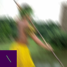
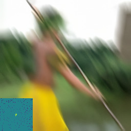
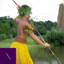
(a) Blurred image Inset: true kernel	(b) Blind-DPS [16], based on alternating minimization Inset: estimated kernel	(c) Kernel-Diff (ours), based on kernel estimation strategy Inset: estimated kernel	(d) Ground Truth

Figure 1: In this paper, we present a novel diffusion-based approach to the blind deconvolution problem. The conventional approaches, such as Blind-DPS, iterate between between kernel and image space minimization. Our approach uses a kernel-first estimation strategy in the context of diffusion models to sample kernels from the conditional distribution $p(\mathbf{k}|\mathbf{y})$.

Although $\text{MAP}_{\mathbf{k}}$ optimization can lead to significantly improved reconstruction (as shown in Figure 1(c) ) it has not been adopted in blind deconvolution solutions, which we surmise because of the intrinsic computational difficulty of the integration in (5).

1.1 Contributions

In this paper, we address the problem with a kernel estimation approach, and we demonstrate that this strategy can be implemented in practice. Our contribution in this paper can be summarized as follows:

1. Using a simple 1D deconvolution example, we demonstrate how the $\text{MAP}_{\mathbf{x},\mathbf{k}}$ framework can be susceptible to local minima while the suggested strategy of $\text{MAP}_{\mathbf{k}}$ does not. Using this example, we show how the marginalization in (5) can be achieved in practice using a non-blind solver.

2. Next, we propose a novel diffusion method, called Kernel-Diffusion (Kernel-Diff) which is based on the design principles outline dabove and is trained to sample from the conditional distribution $p(\mathbf{k}|\mathbf{y})$. This diffusion method coupled with a differentiable non-blind solver achieves state-of-the-art deconvolution performance. We show with numerical experiments on real and synthetic data that the proposed approach creates significant performance improvement.

2 Background

2.1 Diffusion Methods

Diffusion models [64, 28, 72, 65] are a popular generative method which can be used to sample any target diffusion $p_{data}(\mathbf{x})$. The diffusion models begin with a forward process, which starts from $\mathbf{x}_{0}\sim p_{data}(\mathbf{x})$ and gradually adds noise according to variance schedule $\{\beta_{1},\beta_{2},...\beta_{T}\}$, formulated as

$$\mathbf{x}_{t}\sim\mathcal{N}(\sqrt{1-\beta_{t}}\mathbf{x}_{t-1},\beta_{t}\mathbf{I})$$ (6)

at time steps $t\in\{1,2,\dots,T\}$. This forward process converges to $\mathbf{x}_{T}\sim\mathcal{N}(0,\mathbf{I})$. Next, the reverse diffusion process is used to sample from the distribution of $p_{data}$ by starting with $\mathbf{x}_{T}\sim\mathcal{N}(0,\mathbf{I})$ and performing the iterative updates

$$\begin{split}\mathbf{x}_{t-1}=\frac{1}{\sqrt{\alpha_{t}}}\Big{(}\mathbf{x}_{t}-\frac{1-\alpha_{t}}{\sqrt{1-\bar{\alpha_{t}}}}\epsilon_{\theta^{*}}(\mathbf{x}_{t},t)\Big{)}+\sigma_{t}\mathbf{z}_{t},\\ \mathbf{z}_{t}\sim\mathcal{N}(0,\mathbf{I}),\end{split}$$ (7)

where $\alpha_{t}\overset{\text{def}}{=}1-\beta_{t}$, $\bar{\alpha_{t}}\overset{\text{def}}{=}\prod\limits_{i=1}^{t}\alpha_{i}$, and $\epsilon_{\theta^{*}}(\mathbf{x}_{t},t)$ is the trained diffusion network used to learn to denoise $\mathbf{x}_{t}$ at any given time step, trained by minimizing the following loss function.

$$\begin{split}\mathcal{L}(\theta)\overset{\text{def}}{=}\mathbb{E}_{t,\mathbf{x}_{0},\epsilon}\Big{[}\|\epsilon-\epsilon_{\theta}(\sqrt{\bar{\alpha}_{t}}\mathbf{x}_{0}+\sqrt{1-\bar{\alpha_{t}}}\epsilon,t)\|^{2}\Big{]}.\end{split}$$ (8)

Inverse Problems and Diffusion Models. Score based diffusion methods have been extensively used in solving inverse problems [36, 18, 88, 34, 20, 35, 32] by sampling from the posterior $p(\mathbf{x}|\mathbf{y})$ and the corresponding score is calculated using the Bayes’ formula

$$\nabla_{\mathbf{x}_{t}}\log p(\mathbf{x}_{t}|\mathbf{y})=\nabla_{\mathbf{x}_{t}}\log p(\mathbf{x}_{t})+\nabla_{\mathbf{x}_{t}}\log p(\mathbf{y}|\mathbf{x}_{t}).$$ (9)

For example, [30] uses an approximation to the posterior score in (9) and used the Langevin dynamics to sample from the distribution $p(\mathbf{x}|\mathbf{y})$ for the MRI compressed sensing problem; [15, 14] solve the inpainting and super-resolution inverse problems with a modified reverse diffusion scheme which includes a projection step to reduce the consistency metric $\|\mathbf{y}-\mathbf{A}\mathbf{x}\|$ in each iteration; diffusion Posterior Sampling (DPS) [17] solves the noisy inverse problem with alternating diffusion and gradient descent steps.

Image Restoration and Diffusion Models Diffusion models sample from a target distribution while MMSE estimators average over them [35]. As a result, the former has been widely used in image restoration tasks such as deblurring [76], super-resolution [58, 42], and low-light enhancement [74, 31]. For an exhaustive review, we refer the reader to [43].

Guidance in Diffusion Models. Pre-trained diffusion models are often guided at each iteration to produce desired results. This is first proposed in [21] where a classifier gradient is added to each iteration for the final output to belong to the given class. ILVR [13] guides the image diffusion process by constraining the low-frequency information of an image. In the same spirit, [73] guides the diffusion process by refining only the null-space of the corresponding inverse problem. [76] guides a deblurring diffusion model using a pretrained structure module.

2.2 Blind Deconvolution

Traditional blind deconvolution methods can be categorized under the $\text{MAP}_{\mathbf{x},\mathbf{k}}$ framework [9, 79, 2, 63, 52, 45, 80, 67, 10]. For example, [12] uses salient edges for the kernel estimation and then performs image estimation using a Total Variation (TV) prior. [78] refines the kernel estimation process by iterative support detection. [27] performs alternating image and kernel minimization but uses a motion density representation for the blur kernel instead of for pixels. Self-Deblur [54] uses an alternating minimization scheme where a latent deep image prior [70] is used to represent the kernel and image space.

Deep learning methods have replaced the optimization-based approaches and usually involve end-to-end training of image restoration networks [62, 66, 69, 38, 84, 82, 75, 83] using large datasets of pairs of sharp and blurry images, e.g., GoPro [50] and RealBlur [55] datasets. For a more exhaustive review of deep learning based approaches, we refer the readers to [86].

A few methods have utilized the $\text{MAP}_{\mathbf{k}}$ approach, even though not always explicitly stated by the authors. [7] uses a fully convolutional network to predict the Fourier coefficients of the underlying kernel which are used to deconvolve the blurry image in Fourier space. [6, 5] train a Kernel-Prediction Network for all pixels in the image to deal with spatially varying blur. [60] leverages the differentiablity of a non-blind solver [59] to frame the blind deconvolution problem entirely in terms of kernel estimation problems. This strategy is improved by [61] using a key-points based representation to further reduce the dimensionality of the problem.

Toy 1D Deconvolution: Estimate image space $\{a,w\}$ and blur $\sigma$ from $\mathbf{y}(t)$	Loss surface - $\text{MAP}_{a,w,\sigma}$
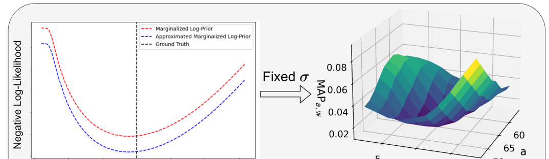
Kernel Estimation from $p(\mathbf{k}|\mathbf{y})$ followed by image estimation

Figure 2: Perils of Alternating Minimization: (Top-Left) Example blind deconvolution setup. Given the blurred signal $y(t)$, we need to recover the underlying latent signal $x(t)$, characterized by $\{a,w\}$, blurred by Gaussian kernel of width $\sigma$ (Top-Right) Loss function for conventional image-kernel minimization, projected in 2D. Alternating minimization of image and kernel can be easily trapped in multiple local minima leading to convergence to false solutions. (Bottom) $\log p(\sigma|y)$ and our suggested approximation from (15). The suggested strategy is to first estimate the kernel by estimating the maximum from $p(\mathbf{k}|\mathbf{y})$ followed by estimation of the image space parameters using the estimated kernel. In this case, we get two convex surfaces and hence the overall scheme is less likely to get trapped in the local minima.

3 Method

3.1 Deconvolution Scheme Analysis

We motivate the proposed method by analyzing a simple 1D deconvolution problem to demonstrate the inherent difficulties of optimization in the alternating minimization framework. We show that minimizing the cost function in (2) is very likely to converge to false minima. We also show the benefits of the $\text{MAP}_{\mathbf{k}}$ strategy.

Simple deconvolution problem. Assume an unknown pulse function $\mathbf{x}_{a,w}(t)$ where $a$ represents the beginning of the pulse and $w$ represents its width. The signal is blurred by a Gaussian pulse $\mathbf{k}_{\sigma}(t)$ where $\sigma$ represents its standard deviation. The resulting signal $\mathbf{y}(t)$ is obtained by blurring the signal $\mathbf{x}(t)$ followed by additive Gaussian noise, i.e.,

$$\mathbf{y}=\mathbf{k}_{\sigma}\circledast\mathbf{x}_{a,w}+\mathcal{N}(0,\beta\mathbf{I}).$$ (10)

Note that that in this setup the image $\mathbf{x}$ and kernel $\mathbf{k}$ are characterized completely be scalars $\{a,w\}$ and $\sigma$, respectively. Therefore, the blind deconvolution problem can be considered as an estimation of the three variables $\{a,w,\sigma\}$.

Alternating Methods versus Kernel Minimization. For the stated example, the conventional alternating minimization approach of $\text{MAP}_{\mathbf{x},\mathbf{k}}$ can be formulated as

$$\begin{split}\hat{a},\hat{w},\hat{\sigma}&=\underset{a,w,\sigma\geq 0}{\text{arg}\max}\Big{[}p(a,w,\sigma|\mathbf{y})\Big{]}\\ &=\underset{a,w,\sigma\geq 0}{\text{arg}\max}\Big{[}\exp\big{(}-\frac{1}{2\beta}\|\mathbf{y}-\mathbf{x}_{a,w}\circledast\mathbf{k}_{\sigma}\|^{2}\big{)}\Big{]}.\end{split}$$ (11)

The equivalent $\text{MAP}_{\mathbf{k}}$ would be first estimating the kernel width $\sigma$ as

$$\begin{split}\hat{\sigma}&=\underset{\sigma\geq 0}{\text{arg}\max}\Big{[}p(\sigma|\mathbf{y})\Big{]}\\ &=\underset{\sigma\geq 0}{\text{arg}\max}\Big{[}\int p(a,w,\sigma|\mathbf{y})da\;dw\Big{]}\\ &=\underset{\sigma\geq 0}{\text{arg}\min}\Big{[}\sum\limits_{a,w\geq 0}\exp\big{[}-\frac{1}{2\beta}\|\mathbf{y}-\mathbf{x}_{a,w}\circledast\mathbf{k}_{\sigma}\|^{2}\big{]}\Big{]},\end{split}$$ (12)

followed by the estimation of $\{a,w\}$:

$$\{\hat{a},\hat{w}\} =\underset{a,w\geq 0}{\text{arg}\min}\Big{[}\|\mathbf{y}-\mathbf{k}_{\hat{\sigma}}\circledast\mathbf{x}_{a,w}\|^{2}\big{]}\Big{]}.$$ (13)

Analysis. In Figure 2, we plot the loss functions corresponding to the two schemes outlined in (11) and (12). We have the following observations according to the loss functions. First, for the joint alternating minimization scheme, the loss function contains many local minima. Even though the global minimum is close to the ground-truth, it is very difficult for a gradient-descent based solver to converge to it unless the random initialization is already very close. Second, for the kernel-based minimization scheme which reduces the search space of the optimization to kernel only, the corresponding loss function has only one minimum, which is also close to the ground-truth. It is very likely that the estimated $\mathbf{x}$, i.e., $\{a,w\}$, will converge to this minimum. Therefore, the kernel-based minimization scheme can consistently produce significantly better results with much lower prediction error than the alternating scheme.

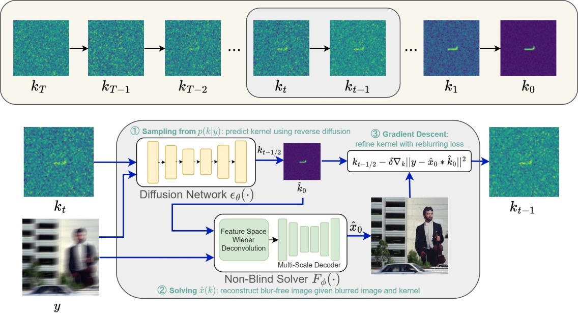
Figure 3: Proposed Kernel-Diff. Each iteration of the proposed kernel-based diffusion contains two sub-steps. First, we perform a reverse diffusion step using the trained diffusion model $\epsilon_{\theta}(\mathbf{k}_{t},\mathbf{y},t)$. Next we plug the temporary kernel estimate $\hat{\mathbf{k}}_{0}$ in the differentiable non-blind solver $F(\cdot)$ and perform a gradient descent update to guide the diffusion process to minimizing the reblurring loss $\|\mathbf{y}-\hat{\mathbf{k}}_{0}\circledast\hat{\mathbf{x}}_{0}\|^{2}$.

3.2 Marginalization of Image Space

In practice, the estimation of $p(\mathbf{k}|\mathbf{y})$ can be difficult because the marginalization in (5) requires a weighted average over all images. We surmise that due to lack of a feasible method to evaluate the likelihood, the approach from [40] was not explored by the imaging community for the blind deconvolution. To mitigate the computational issue, we propose an approximation to the marginalization using a non-blind solver.

Before stating the approximation, we explicitly define a non-blind solver. Given a blurred image $\mathbf{y}$ and the corresponding blur kernel $\mathbf{k}$, we can easily estimate the latent image using a non-blind solver which performs the following image estimation:

$$\hat{\mathbf{x}}(\mathbf{k})=\text{arg}\max\limits_{\mathbf{x}}\Big{[}p(\mathbf{x}|\mathbf{k},\mathbf{y})\Big{]}\overset{\text{def}}{=}F(\mathbf{y},\mathbf{k}).$$ (14)

Traditionally, these non-blind solvers are implemented using an iterative method where the corresponding cost function for MAP estimation in (14) is minimized using gradient descent or proximal updates. Convolutional neural networks with Wiener-deconvolution processing have been used with great success also [23, 59, 22, 51, 11]. The latter provides us with $F(\cdot)$ as a differentiable function with respect to $\mathbf{k}$. The significance of this property will become obvious to the reader in the next subsection.

Now, given our definition of a non-blind solver, we approximate the conditional probability $p(\mathbf{k}|\mathbf{y})$ as follows:

$$\begin{split}p(\mathbf{k}|\mathbf{y})=\int p(\mathbf{x},\mathbf{k}|\mathbf{y})d\mathbf{x}\approx\frac{1}{Z}p(\hat{\mathbf{x}}(\mathbf{k}),\mathbf{k}|\mathbf{y}),\end{split}$$ (15)

where the integration is performed using the Laplace approximation around the mode of the conditional distribution $p(\mathbf{x},\mathbf{k}|\mathbf{y})$ and $Z$ is the constant scaling factor. For a more detailed explanation of this approximation, we refer the readers to Section C of the supplementary document.

For the problem in Section 3.1, $p(\sigma|\mathbf{y})$ can be approximated as

$$p(\sigma|\mathbf{y})\approx\frac{1}{Z^{\prime}}\exp\Big{[}-\frac{1}{2\beta^{2}}\|\mathbf{y}-\mathbf{x}_{a(\sigma),w(\sigma)}\circledast\mathbf{k}_{\sigma}\|^{2}\Big{]},$$ (16)

where $\{a(\sigma),w(\sigma)\}$ represents the best estimate of the image space parameters given $\sigma$ according to (14) and $Z^{\prime}$ is a constant scalar.

Through the approximation in (15), we can now estimate the kernel by maximizing $p(\mathbf{k}|\mathbf{y})$. Firstly, (15) removes the intractable marginalization of the image space making to easier to evaluate the likelihood. Secondly, using the non-blind solver i.e. $\hat{\mathbf{x}}(\mathbf{k})$ allows us to convert the an image-kernel optimization problem to an purely kernel-estimation problem.

3.3 Kernel-Based Diffusion

To sample from $p(\mathbf{k}|\mathbf{y})$, we propose to use a kernel-based diffusion network. This is different from existing methods using diffusion models, e.g., Blind-DPS [16], that resemble the alternating minimization approach, aiming to sample $\{\mathbf{x},\mathbf{k}\}$ from the conditional distribution $p(\mathbf{x},\mathbf{k}|\mathbf{y})$ using implicit score models for image and kernel spaces.

Diffusion Network. We use a modified version of the U-Net architecture as opposed to the one described in [21]. Since we are sampling from a conditional distribution, the diffusion model $\epsilon_{\theta}(\mathbf{k},\mathbf{y},t)$ takes as input both the current kernel estimate $\mathbf{k}_{t}$ and the blurred image $\mathbf{y}$. This is achieved in a similar fashion as [58]. Specifically, our U-Net architecture has two encoders, one for the image $\mathbf{y}$ and the other for the kernel $\mathbf{k}$. In our implementation, we use images of size $256\times 256$ and kernels of size $64\times 64$. At the end of the encoders, the encoded features of the kernel branch are upscaled by a factor of 4 and concatenated to the encoded features of the image branch. The concatenated features are then passed through a common U-Net decoder stage to predict the kernel at the next time step.

The diffusion model $\epsilon_{\theta}(\cdot)$ is trained by minimizing the following loss function:

$$\begin{split}\mathcal{L}_{\text{kernel}}(\theta)&\overset{\text{def}}{=}\mathbb{E}_{t,\mathbf{k},\mathbf{y},\epsilon}\Big{[}\|\epsilon-\epsilon_{\theta}(\sqrt{\bar{\alpha}_{t}}\mathbf{k}+\sqrt{1-\bar{\alpha_{t}}}\epsilon,\mathbf{y},t)\|_{2}^{2}\Big{]}\end{split}$$ (17)

where the expectation is taken over all timesteps $t$, blurred images $\mathbf{y}$ and corresponding blur kernels $\mathbf{k}$. With trained parameters $\theta^{*}$, we sample $p(\mathbf{k}|\mathbf{y})$ using a series of reverse diffusion steps starting from $\mathbf{k}_{T}\sim\mathcal{N}(0,\mathbf{I})$ and the following reverse-diffusion iteration:

$$\mathbf{k}_{t-1}=\frac{1}{\sqrt{\alpha_{t}}}\bigg{(}\mathbf{k}_{t}-\frac{1-\alpha_{t}}{\sqrt{1-\bar{\alpha_{t}}}}\epsilon_{\theta^{*}}(\mathbf{k}_{t},\mathbf{y},t)\bigg{)}+\bar{\sigma}_{t}\mathbf{z}_{t}$$ (18)

Guidance using Non-Blind Solver. Once we have sampled the kernel $\mathbf{k}_{0}$, we estimate the latent image as $\mathbf{x}_{0}=F_{\phi}(\mathbf{y},\mathbf{k}_{0})$, where $F_{\phi}(\cdot)$ is a neural network non-blind solver. There is a vast selection of candidate non-blind solver, including many network-based methods proposed recently [23, 25, 26, 24, 59, 87]. These networks usually convert the blurred images to features space, apply Wiener deconvolution using the kernel followed by converting the deconvolved features into a single image using a decoder.

While diffusion processes are effective in generating samples from the conditional distribution $p(\mathbf{k}|\mathbf{y})$, they do not guarantee minimization of the reblurring loss, i.e., $\|\mathbf{y}-\mathbf{k}\circledast\mathbf{x}\|^{2}$. To minimize reblurring loss while also generating a plausible sample $p(\mathbf{k}|\mathbf{y})$, we guide the reverse diffusion process using the pre-trained non-blind solver as follows.

At step $t$ of the reverse diffusion process, the kernel estimate is given as $\mathbf{k}_{t}$. Using the trained diffusion model $\epsilon_{\theta^{*}}(\mathbf{k}_{t},\mathbf{y},t)$ and $\mathbf{k}_{t}$, we can compute a temporary estimate of the sampled kernel $\mathbf{k}_{0}$ as follows:

$$\hat{\mathbf{k}}_{0}=\frac{1}{\sqrt{\bar{\alpha_{t}}}}\big{(}\mathbf{k}_{t}-\sqrt{1-\bar{\alpha}_{t}}\epsilon_{\theta^{*}}(\mathbf{k}_{t},\mathbf{y},t)\big{)}.$$ (19)

We then estimate the image using this kernel estimate $\hat{\mathbf{k}}_{0}$ by $\hat{\mathbf{x}}_{0}\overset{\text{def}}{=}F(\mathbf{y},\hat{\mathbf{k}}_{0})$, plug into the reblurring loss, and perform gradient descent by

$$\mathbf{k}_{t}\leftarrow\mathbf{k}_{t}-\delta\nabla_{\mathbf{k}_{t}}\|\mathbf{y}-\hat{\mathbf{k}}_{0}\circledast F(\mathbf{y},\hat{\mathbf{k}}_{0})\|^{2}.$$ (20)

1:Input: Blurred Image $\mathbf{y}$, Diffusion UNet $\epsilon_{\theta}(.)$, Non-Blind Solver $F_{\phi}(.)$.

2:// Stage I: Reverse Diffusion

3:$\mathbf{k}_{T}\sim\mathcal{N}(\mathbf{0},\mathbf{I})$

4:for $t=T,\cdot\cdot\cdot,1$ do

5:     $\mathbf{z}_{t}\sim\mathcal{N}(\mathbf{0},\mathbf{I})$

6:     $\mathbf{k}_{t-1/2}=\frac{1}{\sqrt{\alpha_{t}}}\bigg{(}\mathbf{k}_{t}-\frac{1-\alpha_{t}}{\sqrt{1-\bar{\alpha_{t}}}}\epsilon_{\theta}(\mathbf{k}_{t},\mathbf{y},t)\bigg{)}+\sigma_{t}\mathbf{z}_{t}$

7:     $\hat{\mathbf{k}}_{0}=\frac{1}{\sqrt{\bar{\alpha_{t}}}}\big{(}\mathbf{k}_{t}-\sqrt{1-\bar{\alpha}_{t}}\epsilon_{\theta}(\mathbf{k}_{t},\mathbf{y},t)\big{)}$

8:     $\hat{\mathbf{x}}_{0}=F_{\phi}(\mathbf{y},\hat{\mathbf{k}}_{0})$

9:     $\mathbf{k}_{t-1}=\mathbf{k}_{t-1/2}-\delta\nabla_{\mathbf{k}_{t}}(\|\mathbf{y}-\hat{\mathbf{k}}_{0}\circledast\hat{\mathbf{x}}_{0}\|^{2})$

10:end for

11:// Stage II: Refinement

12:for $j=1,\cdot\cdot\cdot,J$ do

13:     $\mathbf{k}_{0}\leftarrow\mathbf{k}_{0}-\delta\nabla_{\mathbf{k}_{0}}(\|\mathbf{y}-\mathbf{k}_{0}\circledast F_{\phi}(\mathbf{y},\mathbf{k}_{0})\|^{2})$

14:end for

15:return $\mathbf{k}_{0}$ and $\mathbf{x}_{0}=F_{\phi}(\mathbf{y},\mathbf{k}_{0})$

Algorithm 1 Kernel-Diff

Overall procedure. We summarize the overall procedure in Algorithm 1 and pictorially represent it in Figure 3. At any given iteration $t$, we first perform reverse diffusion process using the denoising network $\epsilon_{\theta}(\cdot)$ to output $\mathbf{k}_{t-1/2}$ (Step 5). Next, we perform a gradient descent update on $\mathbf{k}_{t-1/2}$ the reblurring loss $\|\mathbf{y}-\hat{\mathbf{k}}_{0}\circledast\hat{\mathbf{x}}_{0}\|^{2}$ (Step 7-9). For further performance boost, once the reverse diffusion process is over, we repeat the gradient descent steps (Step 13) to refine the kernel, similar to Stage II in [61].

4 Experiments

4.1 Experiment Setup

Implementation of Kernel-Diff. The diffusion network we use is a modified U-Net [21]. To train the diffusion model $\epsilon_{\theta}(\mathbf{k}_{t},\mathbf{y},t)$, we generate blurred data using synthetic motion blur kernels, with details of data synthesis to be elaborated in the next section. We assume symmetric boundary conditions during the convolution process. We train the diffusion U-Net architecture for 500,000 iterations with a batch size of 16. For the non-blind solver, we use the pre-trained network Deep Wiener Deconvolution (DWDN) [23] provided by the authors and use it in our scheme without any fine-tuning.

Training Dataset. The diffusion U-Net in Kernel-Diff as well as all methods we compare in our experiments are trained using the same set of blurred and clean image data. We synthesize the blurred images by applying random blur kernels from a kernel database on clean images, similar to [16]. The kernel database consists of 60,000 $64\times 64$ blur kernels generated using an open-sourced motion blur model [4]. For clean images, we use the full-resolution images of Flickr2K [46]. To train the diffusion U-Net for Kernel-Diff, we additionally randomly crop the images to $128\times 128$ patches and augment the data by random horizontal flipping.

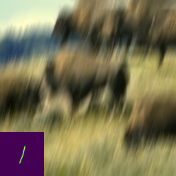
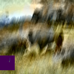
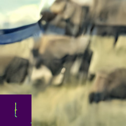
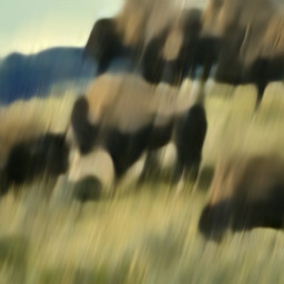
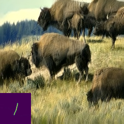
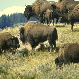
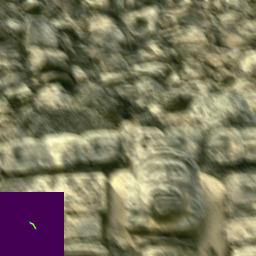
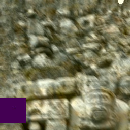
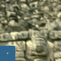
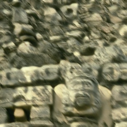
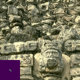
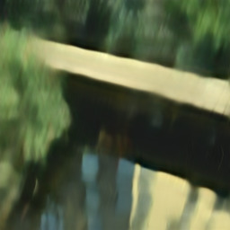
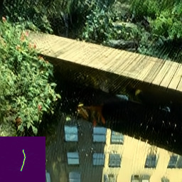
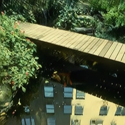
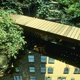
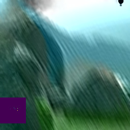
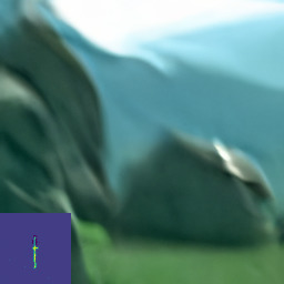
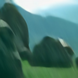
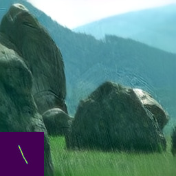
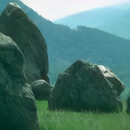
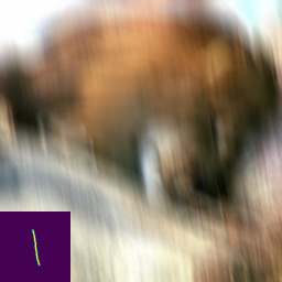
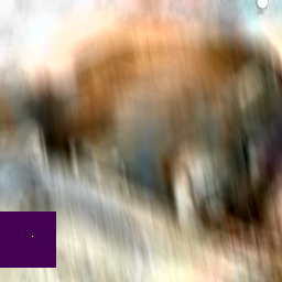
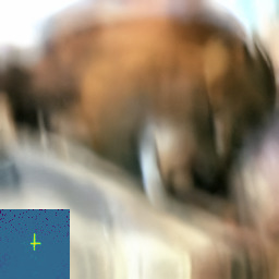
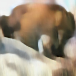
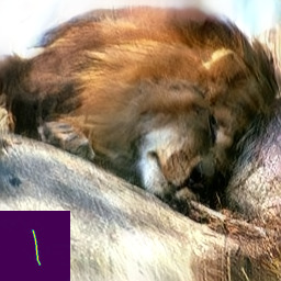
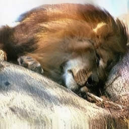
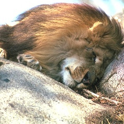
Blurred image Inset: true kernel	Self-Deblur [54]	Blind-DPS [16]	MPR-Net [82]	Kernel-Diff (Ours)	DWDN-Oracle† [23]	Ground Truth

Figure 4: Qualitative Results: Reconstruction results on synthetically blurred images from the BSD100 dataset. For Self-Deblur, Blind-DPS and Kernel-Diff, we show the estimated kernels in inset. ^†DWDN is a non-blind deconvolution method assuming knowledge of the ground-truth kernel; its results are provided for reference only.

4.2 Quantitative Comparison

In this section, we evaluate the proposed method Kernel-Diff on synthetic and real blurred images and compare the performance with other state-of-the-art deconvolution methods. We evaluate our method on the BSD100 and RealBlur datasets as described below along with the following deconvolution/deblurrring methods – Deep Hierarchical Multi-Patch Network (DHMPN) [84], Self-Deblur [54], Blind-DPS [16], MPR-Net [82], and DeblurGANv2 [39]. We use these methods as a representative set of contemporary deconvolution methods which include both iterative and end-to-end trained solutions. For the sake of a fair comparison, we retrain the end-to-end methods using synthetically blurred datasets with details provided in Section D of the supplementary document.

BSD100 Dataset. We first evaluate our method on 100 synthetically blurred images from the BSD dataset [47]. Specifically, we crop out random patches of size $256\times 256$ and then blur them with synthetic motion blur kernels using symmetric boundary conditions. The performance of Kernel-Diff and other deblurring methods is shown in Table 1 along with some qualitative examples in Figure 4. We also compare estimated kernels from Self-Deblur, Blind-DPS and Kernel-Diff in Table 2 using maximum of normalized convolution (MNC) [29].

Method $\rightarrow$ Metric $\downarrow$	DeblurGAN-v2 [39]	Self-Deblur [54]	Blind-DPS [16]	DMPHN [84]	MPR-Net [82]	Kernel-Diff (Ours)	DWDN [23]
PSNR $\uparrow$	15.44	13.53	17.56	18.73	18.49	18.95	22.95
SSIM $\uparrow$	0.396	0.227	0.387	0.427	0.435	0.492	0.810
LPIPS $\downarrow$	0.563	0.665	0.670	0.617	0.632	0.335	0.169
FID $\downarrow$	287.44	259.40	280.53	265.05	265.60	172.33	79.11

Table 1: Performance on BSD100 dataset with synthetic blur. Bold and underline refer to overall and second best blind deconvolution method respectively. DWDN is a non-blind method which knows the ground-truth kernel and is provided as an empirical upper bound only.

Method	Self-Deblur	Blind-DPS	Kernel-Diff
MNC $\uparrow$	0.206	0.283	0.698

Table 2: Kernel Evaluation. Maximum of normalized correlation (MNC) for estimated kernels for iterative blind deconvolution methods.

RealBlur-50. To evaluate our blind deconvolution method on real blurred images, we use the the RealBlur-J dataset [55]. However, since the focus of this paper is only spatially invariant blur and not other forms of blur, we crop random patches of size $256\times 256$ from 50 blurred images in the dataset to reduce the possibility of violating the spatially invarying blur assumption. The results of this comparison are shown in Table 3.

Metric $\rightarrow$ Method $\downarrow$	PSNR $\uparrow$	SSIM $\uparrow$	LPIPS $\downarrow$	FID $\downarrow$
DeblurGAN-v2	14.98	0.583	0.289	129.06
Self-Deblur	16.15	0.483	0.459	172.32
Blind-DPS	19.82	0.607	0.320	175.95
MPR-Net	23.63	0.715	0.213	113.11
Kernel-Diff	25.21	0.779	0.187	116.61

Table 3: Performance on RealBlur-50. Bold and underline refer to overall and second best blind deconvolution method respectively.

4.3 Ablation Study

Effect of Non-Blind Solver Guidance Each iteration of the diffusion consists of two sub-steps: (1) reverse diffusion using the trained dennoiser $\epsilon_{\theta}(\cdot)$ and (2) gradient descent on $\|\mathbf{y}-\hat{\mathbf{k}}_{0}\circledast\hat{\mathbf{x}}_{0}\|^{2}$ using the non-blind solver. In Table 4, we show the effect on performance of the second sub-step. Through the giant gap in performance with and without the guidance, we find that reverse diffusion is insufficient to converge to a good kernel estimate and hence, the experiment justifies the extra complexity required to guide the diffusion process to minimize the reblurring loss.

Metric $\rightarrow$ Method $\downarrow$	PSNR $\uparrow$	SSIM $\uparrow$	LPIPS $\downarrow$	FID $\downarrow$
w/o DWDN	17.83	0.414	0.387	194.58
with DWDN	18.95	0.492	0.335	172.33

w/o non-blind solver guidance	with non-blind solver guidance	DWDN + True kernel

Table 4: Effect of Non-Blind Solver Guidance. Through this ablation study, we examine the effect of the second sub-step in the diffusion process which guides the diffusion process to minimize the reblurring loss using the non-blind solver DWDN [23].

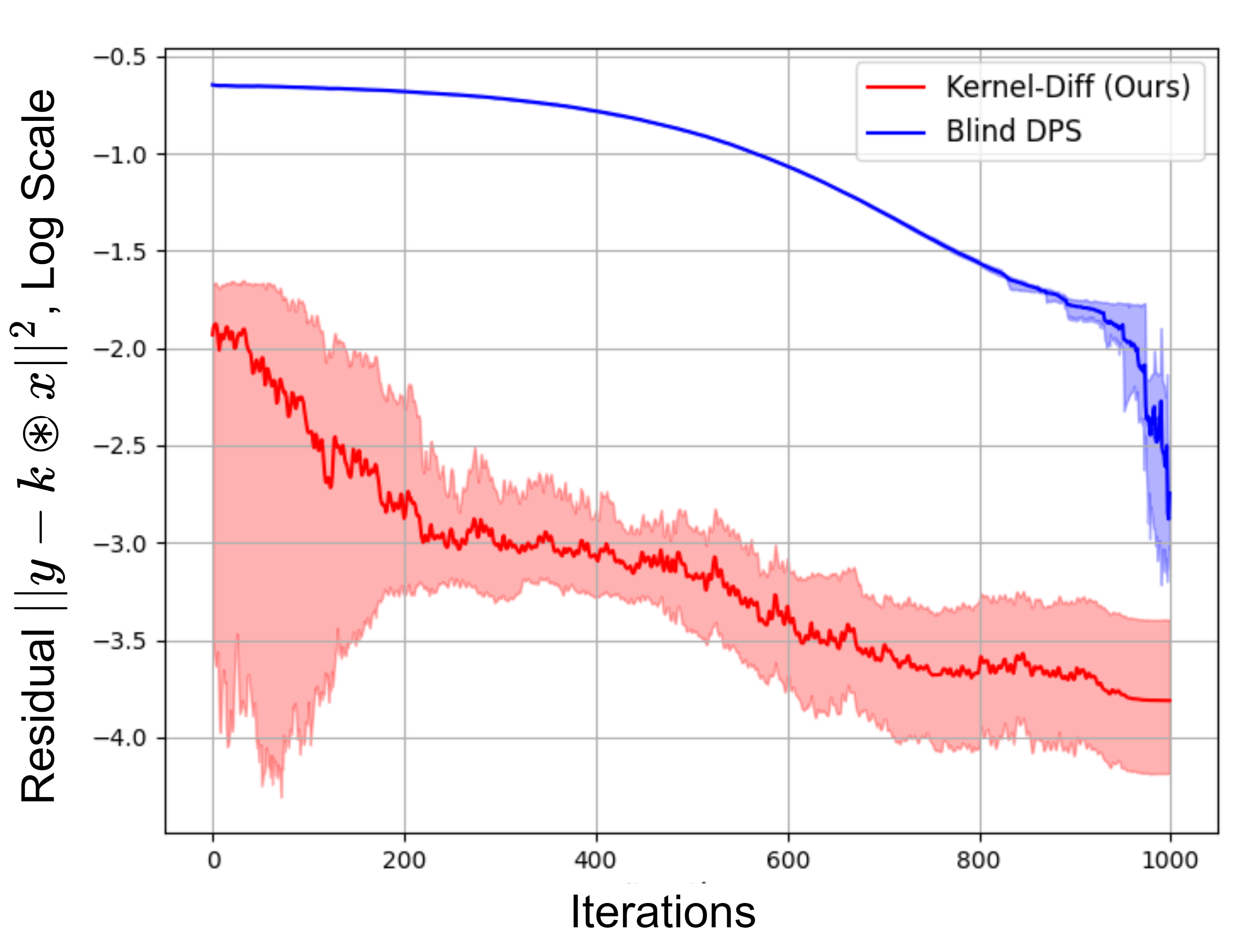
Figure 5: Residual $\|\mathbf{y}-\hat{\mathbf{k}}_{0}\circledast\hat{\mathbf{x}}_{0}\|^{2}$ for Blind-DPS and Kernel-Diff . This experiments confirms our hypothesis that the proposed kernel estimation scheme converges to a better local minimum. The shaded region shows the range of the residual over 50 trials of each scheme.

Reblurring Loss during Diffusion In Section 3.1, we show using a toy example why a alternate minimization approach is more likely to end up in a false local minima. We empirically demonstrate this by comparing the residual across the iterations, i.e., $\|\mathbf{y}-\hat{\mathbf{k}}_{0}\circledast\hat{\mathbf{x}}_{0}\|$ with Blind-DPS [16] in Figure 5. From the figure we observe that the residual in our proposed kernel estimation scheme converges to a solution with a much lower residual value. Assuming the kernel and image likelihoods to be approximately equal for both solutions, we conclude that our method leads to solutions with a higher log-likelihood, and hence, better quality results.

5 Conclusion

In this paper, we proposed Kernel-Diff, a blind deconvolution solution in the tradition of Levin et. al [40]. We first show the pitfalls of conventional minimization using a 1D example and then show how the kernel minimization approach can be implemented in practice using a pre-trained non-blind solver. Using the principles outlined, we propose a guided diffusion method that samples from $p(\mathbf{k}|\mathbf{y})$ to solve the blind deconvolution problem and show extensive numerical experiments on blurred images.

For future work, the method can be refined to deblur images with spatially varying and motion blur i.e. degradation which do not fit the single-blur convolutional model. Alternately, the non-blind solver can be modified to be robust to inaccuracies in kernel estimation.

Supplementary Material

A. Toy Example - Implementation Details

For the toy example proposed in Section 3.1 of the main document, we use the following parameters to generate the loss function plots. The vectors $\mathbf{x}$, $\mathbf{k}$, and $\mathbf{y}$ are assumed to be of length $N=128$. Given this length, we can assume the following bounds on image space parameters $0\leq a\leq 96$ and $0\leq w\leq 32$. We limit the blur kernel width to $0<\sigma\leq 3$. the ground-truth parameters for the experiment are set as $a_{true}=64,w_{true}=10,\sigma_{true}=1.5$

For visualizing the 3-dimensional cost function in Figure 2, we use a modified version of the random projection technique [41] used for the visualization of loss functions in neural networks. Specifically, we take two random normal directions $\mathbf{z}_{1},\mathbf{z}_{2}\sim\mathcal{N}(0,\mathbf{I}_{3})$ corresponding to $\{a,w,\sigma\}$ space . Next we scale the two directions corresponding to the respective scales i.e.

$$\mathbf{t}_{i}=\Big{[}64\mathbf{z}_{i}^{(1)},32\mathbf{z}_{i}^{(2)},\mathbf{z}_{i}^{(3)}\Big{]}\;\;\;i=1,2$$ (21)

Given the random choice of the directions $\mathbf{t}_{1}$ and $\mathbf{t}_{2}$, we need to make sure they are orthogonal, which we achieve by the following operation on $\mathbf{t}_{2}$

$$\mathbf{t}_{2}\leftarrow\mathbf{t}_{2}-\frac{\mathbf{t}_{2}^{T}\mathbf{t}_{1}}{||\mathbf{t}_{1}||^{2}}\mathbf{t}_{1}$$ (22)

Next, we visualize the loss function along the random directions starting from the ground truth parameters $[a_{true},w_{true},\sigma_{true}]$ along the directions $\mathbf{t}_{1},\mathbf{t}_{2}$.

B. Comparison with Levin et. al

In this paper, we show why the kernel estimation strategy from [40] is superior compared to alternating minimization followed by a diffusion-based method incorporating it. Despite the similarities, we come to slightly different conclusions from the original paper which are outlined here.

1. The toy example from [40], presented in Fig. 1 in the paper, depends on the choice of the sparse prior. However, one can argue that $\text{MAP}_{\mathbf{x},\mathbf{k}}$ framework can be useful by a better choice of prior - which is easily possible given deep learning based solutions, which did not exist in 2011. Compared to that, the conclusions arrived in this paper do not depend on the choice of prior since we boil down the optimization problem to the smallest possible subspace i.e. $a,w,\sigma$.

2. While [40] arrives at the conclusion that that the $\text{MAP}_{\mathbf{x},\mathbf{k}}$ strategy favours the no-blur solution, our conclusion is slightly different. Through our choice of the toy-problem, we find that the while the no-blur solution is not favoured, a gradient descent based scheme is still likely to get stuck in false minima, suggesting use of of the $\text{MAP}_{\mathbf{k}}$ framework.

C. Marginalization Approximation

In this section, we describe approximation in Eq. 15 from the main document in detail. We start with the conditional kernel distribution $p(\mathbf{k}|\mathbf{y})$ as a marginalized distribution as follows:

$$p(\mathbf{k}|\mathbf{y})=\int p(\mathbf{x},\mathbf{k}|\mathbf{y})d\mathbf{x}$$ (23)

We approximate the integrand $p(\mathbf{x},\mathbf{k}|\mathbf{y})$ using the Laplace approximation

$$p(\mathbf{x},\mathbf{k}|\mathbf{y})\approx p(\hat{\mathbf{x}},\mathbf{k}|\mathbf{y})\exp\Big{[}-\frac{1}{2}(\mathbf{x}-\hat{\mathbf{x}})^{T}\mathbf{S}^{-1}(\mathbf{x}-\hat{\mathbf{x}})\Big{]}$$ (24)

where

$$\hat{\mathbf{x}}\overset{\text{def}}{=}\underset{\mathbf{x}}{\text{arg}\max}\Big{[}p(\mathbf{x},\mathbf{k}|\mathbf{y})\Big{]}$$ (25)

and

$$\hat{\mathbf{S}}\overset{\text{def}}{=}\Big{[}\frac{\partial^{2}}{\partial\mathbf{x}^{2}}\log p(\mathbf{x},\mathbf{k}|\mathbf{y})\Big{]}_{\mathbf{x}=\hat{\mathbf{x}}}$$ (26)

Applying this approximation to (23),

$$p(\mathbf{k}|\mathbf{y}) \approx\int p(\hat{\mathbf{x}},\mathbf{k}|\mathbf{y})\exp\Big{[}-\frac{1}{2}(\mathbf{x}-\hat{\mathbf{x}})^{T}\mathbf{S}^{-1}(\mathbf{x}-\hat{\mathbf{x}})\Big{]}d\mathbf{x}$$ (27)

$$=p(\hat{\mathbf{x}},\mathbf{k}|\mathbf{y})\int\exp\Big{[}-\frac{1}{2}(\mathbf{x}-\hat{\mathbf{x}})^{T}\mathbf{S}^{-1}(\mathbf{x}-\hat{\mathbf{x}})\Big{]}d\mathbf{x}$$ (28)

$$=p(\hat{\mathbf{x}},\mathbf{k}|\mathbf{y})((2\pi)^{n}|\mathbf{S}|)^{1/2}$$ (29)

here $n$ represents the dimension of the image space $\mathbf{x}$. We further approximate $\mathbf{S}$ to be independent of $\mathbf{x}$, and hence a constant $C$, for sake of computational simplicity. However, future work can focus on providing a better approximation for $|S|$ and include it in the marginalization.

Next we examine the $\hat{\mathbf{x}}$ and its relation to the non-blind solver.

$$\hat{\mathbf{x}} \overset{\text{def}}{=}\underset{\mathbf{x}}{\text{arg}\max}\Big{[}p(\mathbf{x},\mathbf{k}|\mathbf{y})\Big{]}$$ (30)

$$=\underset{\mathbf{x}}{\text{arg}\max}\Big{[}\frac{p(\mathbf{y}|\mathbf{k},\mathbf{x})p(\mathbf{x})p(\mathbf{k})}{p(\mathbf{y})}\Big{]}$$ (31)

$$=\underset{\mathbf{x}}{\text{arg}\max}\Big{[}\frac{p(\mathbf{y}|\mathbf{k},\mathbf{x})p(\mathbf{x})}{p(\mathbf{y})}\Big{]}=\underset{\mathbf{x}}{\text{arg}\max}\Big{[}p(\mathbf{x}|\mathbf{k},\mathbf{y})\Big{]}$$ (32)

Therefore, we have shown that $\hat{\mathbf{x}}$ is the Maximum-A-Posteriori estimate for the non-blind problem problem i.e. estimating $\mathbf{x}$ once the kernel $\mathbf{k}$ is known.

D. Experimental Details

We describe the configurations we use to train the methods for comparison as follows.

DeblurGAN-v2 [39]. We train the DeblurGAN-v2 using the official implementation available with the default configurations, parameters, and loss function. We use the same training scheme as stated in [16] for the majority. The backbone of the generator is a pretrained Inception-ResNet-v2, and we fine-tuned the generator 1.5 million iterations per epoch for 10 epochs. The batch size is 1.

MPR-Net [82], DHMPN [84]: We adopt the official implementations available . We apply the default configurations and their proposed loss function. Again following [16], we use the training scheme to train the model for 30k iterations with a batch size of 3.

E. Kernel-Diff Hyperparameters

Diffusion Hyperparameters For the reverse diffusion process, we use a total of $T=1000$ steps and linear schedule for the noise variance $\{\beta_{t}\}$ as defined in [21]. For training the denoising network $\epsilon_{\theta}(\cdot)$, we use the $\ell_{2}$ norm, instead of the usual $\ell_{1}$ norm, because we empirically observe that training with the latter converges to kernels smaller than the target. This leads to ringing artifacts in the corresponding image output from the non-blind solver $F_{\phi}(\mathbf{y},\mathbf{k})$.

Gradient Step Size: For the reverse diffusion scheme, $\delta$ in Step 9 of Algorithm 1 is chosen similar to the heuristic from Blind-DPS i.e.

$$\delta\overset{\text{def}}{=}\frac{0.1}{\|\mathbf{y}-\hat{\mathbf{k}_{0}}\circledast\hat{\mathbf{x}}_{0}\|^{2}}$$ (33)

This ensure that the gradient descent becomes only aggressive in later stages of the diffusion when we’re closer to the true solution. Conversely, gradient descent is relatively negligible in earlier stages of diffusion.

F. More Qualitative Results

In Figure 6 and 7, we provide more qualitative examples on synthetic and real blurred images reconstructed using our and contemporary methods. For the real blurred images in latter, we use $256\times 256$ patches from the RealBlur [55] and Kohler [37] dataset.

For real-blurred images, we observe that the diffusion model as described in the main document is biased towards kernels generated in . Therefore, to account for the domain gap, we retrain our method Kernel-Diff using motion blur kernels generated from [3] and the corresponding results are shown in Figure 7. Despite the retraining, results from Table 3 of the main document are provided using the original Kernel-Diff. Note that blur in images may not necessarily be spatially invariant due to in-plane camera motion during exposure [77]. This may lead to artifacts caused by deblurring using a single estimated kernel.

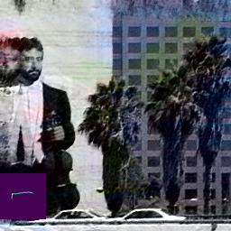
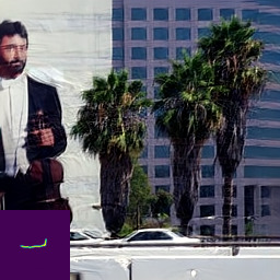
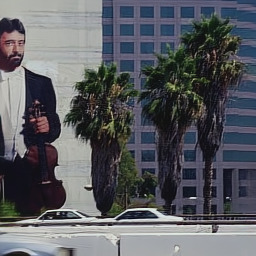
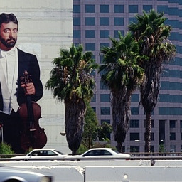
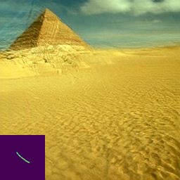
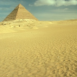
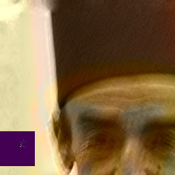
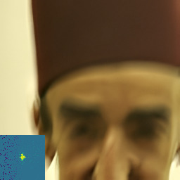
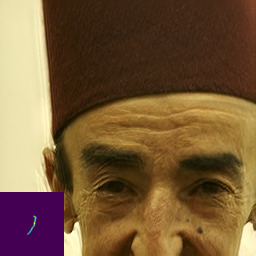
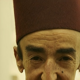
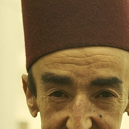
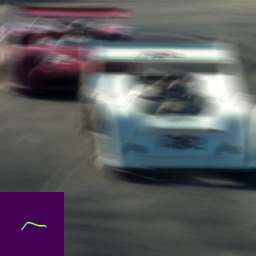
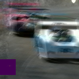
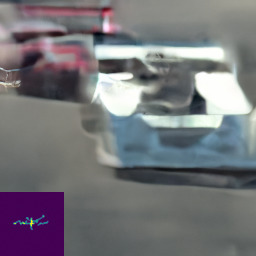
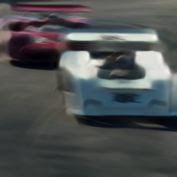
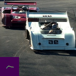
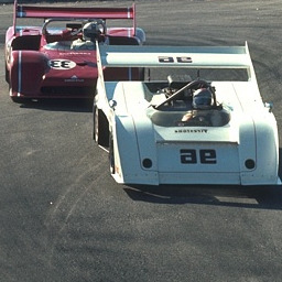
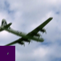
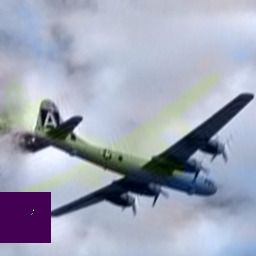
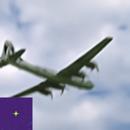
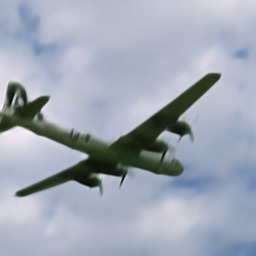
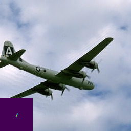
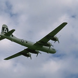
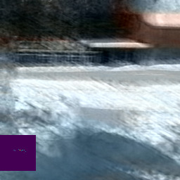
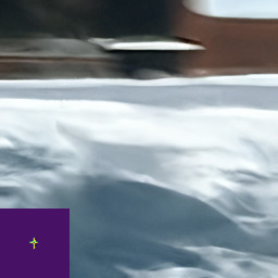
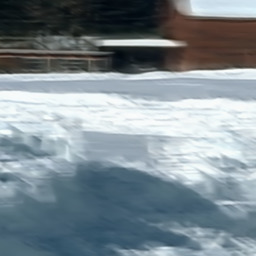
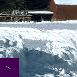
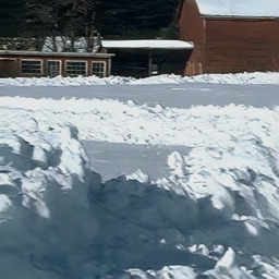
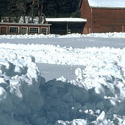
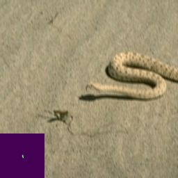
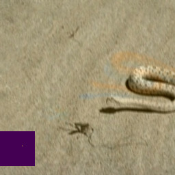
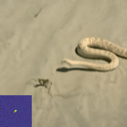
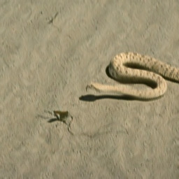
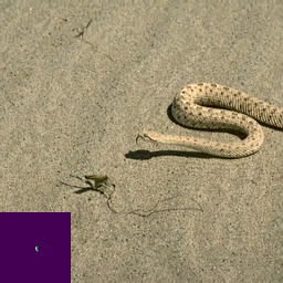
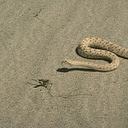
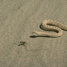
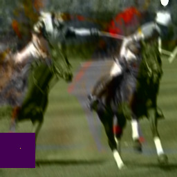
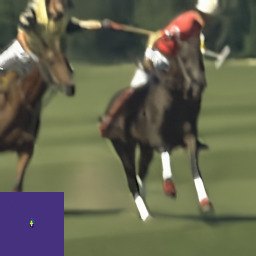
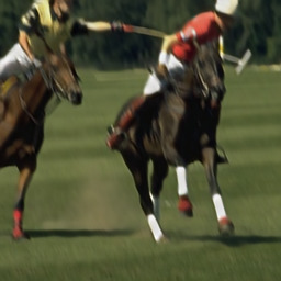
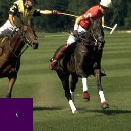
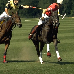
Blurred image Inset: true kernel	Self-Deblur [54]	Blind-DPS [16]	MPR-Net [82]	Kernel-Diff (Ours)	DWDN-Oracle† [23]	Ground Truth

Figure 6: More Qualitative Results from BSD100: Reconstruction results on synthetically blurred images from the BSD100 dataset.

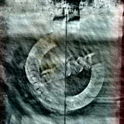
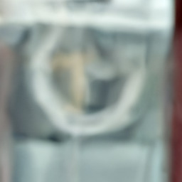
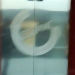
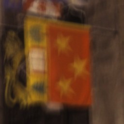
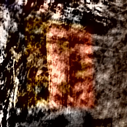
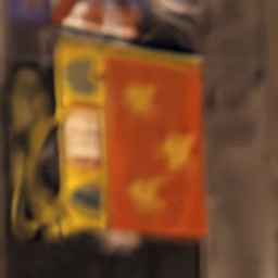
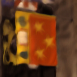
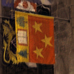
Blurred image	Self-Deblur [54]	Blind-DPS [16]	MPR-Net [82]	Kernel-Diff (Ours)	Ground Truth

Figure 7: Qualitative Results on Real Blurred Images Comparison on real blurred images from the RealBlur [55] and Kohler [37]. We would like to stress that real camera motion is not spatially invariant due to in-plane rotation during exposure. [77]. This may lead to artifacts while deblurring a single blur kernel. Note that even under this model mismatch, our method is able to obtain a relatively good blur kernel estimate for deblurring.

References

- Ahmad et al. [2020] Rizwan Ahmad, Charles A Bouman, Gregery T Buzzard, Stanley Chan, Sizhuo Liu, Edward T Reehorst, and Philip Schniter. Plug-and-play methods for magnetic resonance imaging: Using denoisers for image recovery. IEEE signal processing magazine, 37(1):105–116, 2020.
- Anger et al. [2019] Jérémy Anger, Gabriele Facciolo, and Mauricio Delbracio. Blind image deblurring using the l0 gradient prior. Image processing on line, 9:124–142, 2019.
- Boracchi and Foi [2012] G. Boracchi and A. Foi. Modeling the performance of image restoration from motion blur. Image Processing, IEEE Transactions on, 21(8):3502 –3517, 2012.
- Borodenko [2020] Levi Borodenko. Motion blur, 2020.
- Carbajal et al. [2021] Guillermo Carbajal, Patricia Vitoria, Mauricio Delbracio, Pablo Musé, and José Lezama. Non-uniform blur kernel estimation via adaptive basis decomposition. arXiv preprint arXiv:2102.01026, 2021.
- Carbajal et al. [2023] Guillermo Carbajal, Patricia Vitoria, José Lezama, and Pablo Musé. Blind motion deblurring with pixel-wise kernel estimation via kernel prediction networks. IEEE Transactions on Computational Imaging, 2023.
- Chakrabarti [2016] Ayan Chakrabarti. A neural approach to blind motion deblurring. In Computer Vision–ECCV 2016: 14th European Conference, Amsterdam, The Netherlands, October 11-14, 2016, Proceedings, Part III 14, pages 221–235. Springer, 2016.
- Chan et al. [2016] Stanley H Chan, Xiran Wang, and Omar A Elgendy. Plug-and-play admm for image restoration: Fixed-point convergence and applications. IEEE Transactions on Computational Imaging, 3(1):84–98, 2016.
- Chan and Wong [1998] Tony F Chan and Chiu-Kwong Wong. Total variation blind deconvolution. IEEE transactions on Image Processing, 7(3):370–375, 1998.
- Chen et al. [2019] Liang Chen, Faming Fang, Tingting Wang, and Guixu Zhang. Blind image deblurring with local maximum gradient prior. In Proceedings of the IEEE/CVF Conference on Computer Vision and Pattern Recognition, pages 1742–1750, 2019.
- Chen et al. [2023] Liang Chen, Jiawei Zhang, Zhenhua Li, Yunxuan Wei, Faming Fang, Jimmy Ren, and Jinshan Pan. Deep richardson–lucy deconvolution for low-light image deblurring. International Journal of Computer Vision, pages 1–18, 2023.
- Cho and Lee [2009] Sunghyun Cho and Seungyong Lee. Fast motion deblurring. ACM Transactions on Graphics, pages 1–8, 2009.
- Choi et al. [2021] Jooyoung Choi, Sungwon Kim, Yonghyun Jeong, Youngjune Gwon, and Sungroh Yoon. Ilvr: Conditioning method for denoising diffusion probabilistic models. In Proceedings of the IEEE/CVF International Conference on Computer Vision (ICCV), pages 14367–14376, 2021.
- Chung et al. [2022a] Hyungjin Chung, Byeongsu Sim, Dohoon Ryu, and Jong Chul Ye. Improving diffusion models for inverse problems using manifold constraints. Advances in Neural Information Processing Systems, 35:25683–25696, 2022a.
- Chung et al. [2022b] Hyungjin Chung, Byeongsu Sim, and Jong Chul Ye. Come-closer-diffuse-faster: Accelerating conditional diffusion models for inverse problems through stochastic contraction. In Proceedings of the IEEE/CVF Conference on Computer Vision and Pattern Recognition, pages 12413–12422, 2022b.
- Chung et al. [2023a] Hyungjin Chung, Jeongsol Kim, Sehui Kim, and Jong Chul Ye. Parallel diffusion models of operator and image for blind inverse problems. In Proceedings of the IEEE/CVF Conference on Computer Vision and Pattern Recognition, pages 6059–6069, 2023a.
- Chung et al. [2023b] Hyungjin Chung, Jeongsol Kim, Michael Thompson Mccann, Marc Louis Klasky, and Jong Chul Ye. Diffusion posterior sampling for general noisy inverse problems. In The Eleventh International Conference on Learning Representations, 2023b.
- Chung et al. [2023c] Hyungjin Chung, Dohoon Ryu, Michael T McCann, Marc L Klasky, and Jong Chul Ye. Solving 3d inverse problems using pre-trained 2d diffusion models. In Proceedings of the IEEE/CVF Conference on Computer Vision and Pattern Recognition, pages 22542–22551, 2023c.
- Cohen et al. [2021] Regev Cohen, Michael Elad, and Peyman Milanfar. Regularization by denoising via fixed-point projection (red-pro). SIAM Journal on Imaging Sciences, 14(3):1374–1406, 2021.
- Daras et al. [2023] Giannis Daras, Mauricio Delbracio, Hossein Talebi, Alex Dimakis, and Peyman Milanfar. Soft diffusion: Score matching with general corruptions. Transactions on Machine Learning Research, 2023.
- Dhariwal and Nichol [2021] Prafulla Dhariwal and Alexander Nichol. Diffusion models beat gans on image synthesis. Advances in neural information processing systems, 34:8780–8794, 2021.
- Dong et al. [2018] Jiangxin Dong, Jinshan Pan, Deqing Sun, Zhixun Su, and Ming-Hsuan Yang. Learning data terms for non-blind deblurring. In Proceedings of the European Conference on Computer Vision (ECCV), pages 748–763, 2018.
- Dong et al. [2020] Jiangxin Dong, Stefan Roth, and Bernt Schiele. Deep wiener deconvolution: Wiener meets deep learning for image deblurring. Advances in Neural Information Processing Systems, 33:1048–1059, 2020.
- Dong et al. [2021] Jiangxin Dong, Stefan Roth, and Bernt Schiele. Learning spatially-variant map models for non-blind image deblurring. In Proceedings of the IEEE/CVF conference on computer vision and pattern recognition, pages 4886–4895, 2021.
- Eboli et al. [2020] Thomas Eboli, Jian Sun, and Jean Ponce. End-to-end interpretable learning of non-blind image deblurring. In Computer Vision–ECCV 2020: 16th European Conference, Glasgow, UK, August 23–28, 2020, Proceedings, Part XVII 16, pages 314–331. Springer, 2020.
- Gong et al. [2020] Dong Gong, Zhen Zhang, Qinfeng Shi, Anton van den Hengel, Chunhua Shen, and Yanning Zhang. Learning deep gradient descent optimization for image deconvolution. IEEE transactions on neural networks and learning systems, 31(12):5468–5482, 2020.
- Gupta et al. [2010] Ankit Gupta, Neel Joshi, C Lawrence Zitnick, Michael Cohen, and Brian Curless. Single image deblurring using motion density functions. In Computer Vision–ECCV 2010: 11th European Conference on Computer Vision, Heraklion, Crete, Greece, September 5-11, 2010, Proceedings, Part I 11, pages 171–184. Springer, 2010.
- Ho et al. [2020] Jonathan Ho, Ajay Jain, and Pieter Abbeel. Denoising diffusion probabilistic models. Advances in neural information processing systems, 33:6840–6851, 2020.
- Hu and Yang [2012] Zhe Hu and Ming-Hsuan Yang. Good regions to deblur. In Computer Vision–ECCV 2012: 12th European Conference on Computer Vision, Florence, Italy, October 7-13, 2012, Proceedings, Part V 12, pages 59–72. Springer, 2012.
- Jalal et al. [2021] Ajil Jalal, Marius Arvinte, Giannis Daras, Eric Price, Alexandros G Dimakis, and Jon Tamir. Robust compressed sensing mri with deep generative priors. Advances in Neural Information Processing Systems, 34:14938–14954, 2021.
- Jiang et al. [2023] Hai Jiang, Ao Luo, Songchen Han, Haoqiang Fan, and Shuaicheng Liu. Low-light image enhancement with wavelet-based diffusion models. arXiv preprint arXiv:2306.00306, 2023.
- Kadkhodaie and Simoncelli [2021] Zahra Kadkhodaie and Eero Simoncelli. Stochastic solutions for linear inverse problems using the prior implicit in a denoiser. Advances in Neural Information Processing Systems, 34:13242–13254, 2021.
- Kamilov et al. [2017] Ulugbek S Kamilov, Hassan Mansour, and Brendt Wohlberg. A plug-and-play priors approach for solving nonlinear imaging inverse problems. IEEE Signal Processing Letters, 24(12):1872–1876, 2017.
- Kawar et al. [2021a] Bahjat Kawar, Gregory Vaksman, and Michael Elad. Snips: Solving noisy inverse problems stochastically. Advances in Neural Information Processing Systems, 34:21757–21769, 2021a.
- Kawar et al. [2021b] Bahjat Kawar, Gregory Vaksman, and Michael Elad. Stochastic image denoising by sampling from the posterior distribution. In Proceedings of the IEEE/CVF International Conference on Computer Vision, pages 1866–1875, 2021b.
- Kawar et al. [2022] Bahjat Kawar, Michael Elad, Stefano Ermon, and Jiaming Song. Denoising diffusion restoration models. Advances in Neural Information Processing Systems, 35:23593–23606, 2022.
- Köhler et al. [2012] Rolf Köhler, Michael Hirsch, Betty Mohler, Bernhard Schölkopf, and Stefan Harmeling. Recording and playback of camera shake: Benchmarking blind deconvolution with a real-world database. In Computer Vision–ECCV 2012: 12th European Conference on Computer Vision, Florence, Italy, October 7-13, 2012, Proceedings, Part VII 12, pages 27–40. Springer, 2012.
- Kupyn et al. [2018] Orest Kupyn, Volodymyr Budzan, Mykola Mykhailych, Dmytro Mishkin, and Jiri Matas. Deblurgan: Blind motion deblurring using conditional adversarial networks. In 2018 IEEE/CVF Conference on Computer Vision and Pattern Recognition, pages 8183–8192, 2018.
- Kupyn et al. [2019] Orest Kupyn, Tetiana Martyniuk, Junru Wu, and Zhangyang Wang. Deblurgan-v2: Deblurring (orders-of-magnitude) faster and better. In The IEEE International Conference on Computer Vision (ICCV), 2019.
- Levin et al. [2011] Anat Levin, Yair Weiss, Fredo Durand, and William T Freeman. Understanding blind deconvolution algorithms. IEEE Transactions on Pattern Analysis and Machine Intelligence, 33(12):2354–2367, 2011.
- Li et al. [2018] Hao Li, Zheng Xu, Gavin Taylor, Christoph Studer, and Tom Goldstein. Visualizing the loss landscape of neural nets. Advances in neural information processing systems, 31, 2018.
- Li et al. [2022] Haoying Li, Yifan Yang, Meng Chang, Shiqi Chen, Huajun Feng, Zhihai Xu, Qi Li, and Yueting Chen. Srdiff: Single image super-resolution with diffusion probabilistic models. Neurocomputing, 479:47–59, 2022.
- Li et al. [2023] Xin Li, Yulin Ren, Xin Jin, Cuiling Lan, Xingrui Wang, Wenjun Zeng, Xinchao Wang, and Zhibo Chen. Diffusion models for image restoration and enhancement–a comprehensive survey. arXiv preprint arXiv:2308.09388, 2023.
- Li et al. [2019] Yuelong Li, Mohammad Tofighi, Vishal Monga, and Yonina C Eldar. An algorithm unrolling approach to deep image deblurring. In ICASSP 2019-2019 IEEE International Conference on Acoustics, Speech and Signal Processing (ICASSP), pages 7675–7679. IEEE, 2019.
- Li et al. [2020] Yuelong Li, Mohammad Tofighi, Junyi Geng, Vishal Monga, and Yonina C Eldar. Efficient and interpretable deep blind image deblurring via algorithm unrolling. IEEE Transactions on Computational Imaging, 6:666–681, 2020.
- Lim et al. [2017] Bee Lim, Sanghyun Son, Heewon Kim, Seungjun Nah, and Kyoung Mu Lee. Enhanced deep residual networks for single image super-resolution. In Proceedings of the IEEE/CVF Conference on Computer Vision and Pattern Recognition (CVPR) Workshops, 2017.
- Martin et al. [2001] D. Martin, C. Fowlkes, D. Tal, and J. Malik. A database of human segmented natural images and its application to evaluating segmentation algorithms and measuring ecological statistics. In Proc. 8th Int’l Conf. Computer Vision, pages 416–423, 2001.
- Monga et al. [2021] Vishal Monga, Yuelong Li, and Yonina C Eldar. Algorithm unrolling: Interpretable, efficient deep learning for signal and image processing. IEEE Signal Processing Magazine, 38(2):18–44, 2021.
- Murata et al. [2023] Naoki Murata, Koichi Saito, Chieh-Hsin Lai, Yuhta Takida, Toshimitsu Uesaka, Yuki Mitsufuji, and Stefano Ermon. Gibbsddrm: A partially collapsed gibbs sampler for solving blind inverse problems with denoising diffusion restoration. arXiv preprint arXiv:2301.12686, 2023.
- Nah et al. [2017] Seungjun Nah, Tae Hyun Kim, and Kyoung Mu Lee. Deep multi-scale convolutional neural network for dynamic scene deblurring. In Proceedings of the IEEE conference on computer vision and pattern recognition, pages 3883–3891, 2017.
- Nan and Ji [2020] Yuesong Nan and Hui Ji. Deep learning for handling kernel/model uncertainty in image deconvolution. In Proceedings of the IEEE/CVF conference on computer vision and pattern recognition, pages 2388–2397, 2020.
- Pan et al. [2016] Jinshan Pan, Deqing Sun, Hanspeter Pfister, and Ming-Hsuan Yang. Blind image deblurring using dark channel prior. In Proceedings of the IEEE conference on computer vision and pattern recognition, pages 1628–1636, 2016.
- Reehorst and Schniter [2018] Edward T Reehorst and Philip Schniter. Regularization by denoising: Clarifications and new interpretations. IEEE transactions on computational imaging, 5(1):52–67, 2018.
- Ren et al. [2020] Dongwei Ren, Kai Zhang, Qilong Wang, Qinghua Hu, and Wangmeng Zuo. Neural blind deconvolution using deep priors. In Proceedings of the IEEE/CVF Conference on Computer Vision and Pattern Recognition, pages 3341–3350, 2020.
- Rim et al. [2020] Jaesung Rim, Haeyun Lee, Jucheol Won, and Sunghyun Cho. Real-world blur dataset for learning and benchmarking deblurring algorithms. In Proceedings of the European Conference on Computer Vision (ECCV), 2020.
- Romano et al. [2017] Yaniv Romano, Michael Elad, and Peyman Milanfar. The little engine that could: Regularization by denoising (red). SIAM Journal on Imaging Sciences, 10(4):1804–1844, 2017.
- Rond et al. [2016] Arie Rond, Raja Giryes, and Michael Elad. Poisson inverse problems by the plug-and-play scheme. Journal of Visual Communication and Image Representation, 41:96–108, 2016.
- Saharia et al. [2021] Chitwan Saharia, Jonathan Ho, William Chan, Tim Salimans, David J Fleet, and Mohammad Norouzi. Image super-resolution via iterative refinement. arXiv:2104.07636, 2021.
- Sanghvi et al. [2022a] Yash Sanghvi, Abhiram Gnanasambandam, and Stanley H Chan. Photon limited non-blind deblurring using algorithm unrolling. IEEE Transactions on Computational Imaging, 8:851–864, 2022a.
- Sanghvi et al. [2022b] Yash Sanghvi, Abhiram Gnanasambandam, Zhiyuan Mao, and Stanley H Chan. Photon-limited blind deconvolution using unsupervised iterative kernel estimation. IEEE Transactions on Computational Imaging, 8:1051–1062, 2022b.
- Sanghvi et al. [2023] Yash Sanghvi, Zhiyuan Mao, and Stanley H Chan. Structured kernel estimation for photon-limited deconvolution. In Proceedings of the IEEE/CVF Conference on Computer Vision and Pattern Recognition, pages 9863–9872, 2023.
- Schuler et al. [2015] Christian J Schuler, Michael Hirsch, Stefan Harmeling, and Bernhard Schölkopf. Learning to deblur. IEEE transactions on pattern analysis and machine intelligence, 38(7):1439–1451, 2015.
- Shan et al. [2008] Qi Shan, Jiaya Jia, and Aseem Agarwala. High-quality motion deblurring from a single image. ACM Transactions on Graphics, 27(3):1–10, 2008.
- Sohl-Dickstein et al. [2015] Jascha Sohl-Dickstein, Eric Weiss, Niru Maheswaranathan, and Surya Ganguli. Deep unsupervised learning using nonequilibrium thermodynamics. In International conference on machine learning, pages 2256–2265. PMLR, 2015.
- Song et al. [2021] Yang Song, Jascha Sohl-Dickstein, Diederik P Kingma, Abhishek Kumar, Stefano Ermon, and Ben Poole. Score-based generative modeling through stochastic differential equations. In International Conference on Learning Representations, 2021.
- Sun et al. [2015] Jian Sun, Wenfei Cao, Zongben Xu, and Jean Ponce. Learning a convolutional neural network for non-uniform motion blur removal. In Proceedings of the IEEE conference on computer vision and pattern recognition, pages 769–777, 2015.
- Sun et al. [2013] Libin Sun, Sunghyun Cho, Jue Wang, and James Hays. Edge-based blur kernel estimation using patch priors. In IEEE international conference on computational photography (ICCP), pages 1–8. IEEE, 2013.
- Sun et al. [2019] Yu Sun, Brendt Wohlberg, and Ulugbek S Kamilov. An online plug-and-play algorithm for regularized image reconstruction. IEEE Transactions on Computational Imaging, 5(3):395–408, 2019.
- Tao et al. [2018] Xin Tao, Hongyun Gao, Xiaoyong Shen, Jue Wang, and Jiaya Jia. Scale-recurrent network for deep image deblurring. In Proceedings of the IEEE conference on computer vision and pattern recognition, pages 8174–8182, 2018.
- Ulyanov et al. [2018] Dmitry Ulyanov, Andrea Vedaldi, and Victor Lempitsky. Deep image prior. In Proceedings of the IEEE conference on computer vision and pattern recognition, pages 9446–9454, 2018.
- Venkatakrishnan et al. [2013] Singanallur V Venkatakrishnan, Charles A Bouman, and Brendt Wohlberg. Plug-and-play priors for model based reconstruction. In 2013 IEEE global conference on signal and information processing, pages 945–948. IEEE, 2013.
- Vincent [2011] Pascal Vincent. A connection between score matching and denoising autoencoders. Neural computation, 23(7):1661–1674, 2011.
- Wang et al. [2023a] Yinhuai Wang, Jiwen Yu, and Jian Zhang. Zero-shot image restoration using denoising diffusion null-space model. The Eleventh International Conference on Learning Representations, 2023a.
- Wang et al. [2023b] Yufei Wang, Yi Yu, Wenhan Yang, Lanqing Guo, Lap-Pui Chau, Alex C Kot, and Bihan Wen. Exposurediffusion: Learning to expose for low-light image enhancement. In Proceedings of the IEEE/CVF International Conference on Computer Vision, pages 12438–12448, 2023b.
- Wang et al. [2021] Zhendong Wang, Xiaodong Cun, Jianmin Bao, and Jianzhuang Liu. Uformer: A general u-shaped transformer for image restoration. in 2022 ieee. In CVF Conference on Computer Vision and Pattern Recognition (CVPR), pages 17662–17672, 2021.
- Whang et al. [2022] Jay Whang, Mauricio Delbracio, Hossein Talebi, Chitwan Saharia, Alexandros G Dimakis, and Peyman Milanfar. Deblurring via stochastic refinement. In Proceedings of the IEEE/CVF Conference on Computer Vision and Pattern Recognition, pages 16293–16303, 2022.
- Whyte et al. [2012] Oliver Whyte, Josef Sivic, Andrew Zisserman, and Jean Ponce. Non-uniform deblurring for shaken images. International journal of computer vision, 98:168–186, 2012.
- Xu and Jia [2010] Li Xu and Jiaya Jia. Two-phase kernel estimation for robust motion deblurring. In European Conference on Computer Vision, pages 157–170. Springer, 2010.
- Xu et al. [2013] Li Xu, Shicheng Zheng, and Jiaya Jia. Unnatural l0 sparse representation for natural image deblurring. In Proceedings of the IEEE conference on computer vision and pattern recognition, pages 1107–1114, 2013.
- Yan et al. [2017] Yanyang Yan, Wenqi Ren, Yuanfang Guo, Rui Wang, and Xiaochun Cao. Image deblurring via extreme channels prior. In Proceedings of the IEEE Conference on Computer Vision and Pattern Recognition, pages 4003–4011, 2017.
- yang et al. [2016] yan yang, Jian Sun, Huibin Li, and Zongben Xu. Deep admm-net for compressive sensing mri. In Advances in Neural Information Processing Systems. Curran Associates, Inc., 2016.
- Zamir et al. [2021] Syed Waqas Zamir, Aditya Arora, Salman Khan, Munawar Hayat, Fahad Shahbaz Khan, Ming-Hsuan Yang, and Ling Shao. Multi-stage progressive image restoration. In Proceedings of the IEEE/CVF conference on computer vision and pattern recognition, pages 14821–14831, 2021.
- Zamir et al. [2022] Syed Waqas Zamir, Aditya Arora, Salman Khan, Munawar Hayat, Fahad Shahbaz Khan, and Ming-Hsuan Yang. Restormer: Efficient transformer for high-resolution image restoration. In Proceedings of the IEEE/CVF conference on computer vision and pattern recognition, pages 5728–5739, 2022.
- Zhang et al. [2019] Hongguang Zhang, Yuchao Dai, Hongdong Li, and Piotr Koniusz. Deep stacked hierarchical multi-patch network for image deblurring. In Proceedings of the IEEE/CVF Conference on Computer Vision and Pattern Recognition, pages 5978–5986, 2019.
- Zhang et al. [2017] Kai Zhang, Wangmeng Zuo, Shuhang Gu, and Lei Zhang. Learning deep cnn denoiser prior for image restoration. In Proceedings of the IEEE conference on computer vision and pattern recognition, pages 3929–3938, 2017.
- Zhang et al. [2022] Kaihao Zhang, Wenqi Ren, Wenhan Luo, Wei-Sheng Lai, Björn Stenger, Ming-Hsuan Yang, and Hongdong Li. Deep image deblurring: A survey. International Journal of Computer Vision, 130(9):2103–2130, 2022.
- Zhang et al. [2023] Zhihong Zhang, Yuxiao Cheng, Jinli Suo, Liheng Bian, and Qionghai Dai. Infwide: Image and feature space wiener deconvolution network for non-blind image deblurring in low-light conditions. IEEE Transactions on Image Processing, 32:1390–1402, 2023.
- Zhu et al. [2023] Yuanzhi Zhu, Kai Zhang, Jingyun Liang, Jiezhang Cao, Bihan Wen, Radu Timofte, and Luc Van Gool. Denoising diffusion models for plug-and-play image restoration. In Proceedings of the IEEE/CVF Conference on Computer Vision and Pattern Recognition, pages 1219–1229, 2023.