Pulse vaccination in a modified SIR model:
global dynamics, bifurcations and seasonality

Abstract.

We analyze a periodically-forced dynamical system inspired by the SIR model with pulse vaccination. We fully characterize its dynamics according to the proportion $p$ of vaccinated individuals and the time $T$ between doses. If the basic reproduction number is less than 1 (i.e. $\mathcal{R}_{p}<1$), then we obtain precise conditions for the existence and global stability of a disease-free $T$-periodic solution. Otherwise, if $\mathcal{R}_{p}>1$, then a globally stable $T$-periodic solution emerges with positive coordinates. We draw a bifurcation diagram $(T,p)$ and we describe the associated bifurcations. We also find analytically and numerically chaotic dynamics by adding seasonality to the disease transmission rate. In a realistic context, low vaccination coverage and intense seasonality may result in unpredictable dynamics. Previous experiments have suggested chaos in periodically-forced biological impulsive models, but no analytic proof has been given.

1. Introduction

Mathematical models have proved to be a useful tool in epidemiology, providing insights into the dynamics of infectious diseases and giving insights to improve strategies to combat their spread [1, 2]. In particular, the SIR model, which classifies individuals into Susceptibles ($S$), Infectious ($I$) and Recovered ($R$), has been extensively used [3, 4].

A prompt response is crucial once a disease emerges in a population. A range of approaches have been explored [5, 6, 7], with vaccination being one of the most effective ways to stop the progression [8, 9].

Among the vaccination strategies in SIR models, we can point out three types:

1. constant vaccination, where a fixed proportion of the population is vaccinated [10, 11, 12], as in the administration of the BCG vaccine against tuberculosis to newborns;

2. pulse vaccination, which involves vaccinating a percentage of the Susceptible individuals periodically [12, 13, 14, 15], similar to mass vaccination campaigns using oral polio vaccine in areas with polio outbreaks; and

3. mixed vaccination [12], as the hepatitis B vaccination program, which starts with one shot immediately after birth, followed by subsequent shots.

Identifying the most suitable vaccination strategy represents a challenge, requiring considerations of effectiveness and costs associated with public health policies. Although considerable literature considers the logistic growth of the susceptible population, seasonality, and the effect of vaccination, the combination of them remains unexplored.

Pulse vaccination over a proportion $p$ of the population may be a strategy to stop the progression of an infectious disease [12, 15, 16, 17]. The effective strategy must be in a way that the proportion $p$ of vaccination is at the target level needed for the disease eradication, and the time $T$ between doses must be suitable. Finding the most appropriate pair $(T,p)$ for specific models is an open problem.

Some authors highlight the presence of seasonal forces in epidemic models such as school holidays, climate change, and political decisions [18]. While the seasonal impact is negligible for some diseases, for others such as childhood illnesses and influenza, it may have dramatic consequences in the dynamics of the models [19]. Differential equations adjust transmission rates using periodic functions [20], making them more complex than standard models but also more realistic [21, 22].

This work focuses on the application of a modified SIR model with pulse vaccination and subject to seasonality, a promising unexplored field.

State of the art

An optimal design of a vaccination program requires, apart from financial and logistical considerations, subtle results in epidemiology that are currently not available in the literature. Several works focus on the study of epidemiological models with pulse vaccination.

In 2002, Lu et al. [15] explored constant and pulse vaccination strategies in an SIR model with vertical and horizontal transmission. Authors showed that the effectiveness of the vaccination strategy depended on the interval between boosters. They observed that the high susceptibility in the offspring of infected parents accelerates stabilisation, emphasising the importance of parental health. Numerical simulations supported their findings.

Wang [23] studied the periodic oscillation of seasonally forced epidemiological models with pulse vaccination. Using Mawhin’s coincidence degree method, the author confirmed the existence of positive periodic solutions for these SIR models with pulse vaccination. The effectiveness of this vaccination strategy was supported by numerical simulations. For further investigation using Mawhin’s degree of coincidence method, we address the reader to [24, 25, 26, 27] for a more in-depth understanding.

Meng and Chen [16] analyzed a SIR epidemic model with vertical and horizontal disease transmission. The authors also revealed that under some conditions, the system is permanent. Moreover, for $\mathcal{R}_{0}>1$ (basic reproduction number), the system under consideration exhibits positive periodic solutions.

In 2022, authors of [19] investigated a periodically-forced dynamical system inspired by the SIR model. They provided a rigorous proof of the existence of observable chaos, expressed as persistent strange attractors on subsets of parameters for $\mathcal{R}_{0}<1$, where $\mathcal{R}_{0}$ stands for the basic reproduction number. Their results are in line with the empirical belief that intense seasonality can induce chaotic behavior in biological systems.

Achieviements

The present work provides insights into the interplay between seasonality, impulsive differential equations and the presence of horseshoes in periodically-forced epidemic models. The main goals of this article are the rigorous proof of the following assertions:

1. in the absence of seasonality, the model goes through five scenarios when varying the parameters of the period $T$ of the vaccine, and the proportion of Susceptible individuals vaccinated $p$;

2. in the absence of seasonality, we design an optimum vaccination program as a function of the period $T$ of pulse vaccination and the proportion $p$ of Susceptible individuals that need to be vaccinated to control the disease;

3. under the presence of seasonality in the rate transmission rate of the disease, the system may behave chaotically and exhibits topological horseshoes.

The bifurcations between the different scenarios have been identified and explored. All the results are illustrated with numerical simulations.

Structure

In this paper, we analyze a modified SIR model to study the impact of the pulse vaccination strategy with and without seasonality. Section 2 provides fundamental insights into impulsive differential equations and the important concepts of periodic solutions and stability. Section 3 introduces our model (with and without vaccination and with and without seasonality) and outlines our hypotheses and motivations. Also, in this section, we present our two main results. From Section 4 to Section 7, we analyze our model from a mathematical point of view: we find the fixed points of the associated stroboscopic maps, compute the basic reproduction number, and evaluate the local stability of the disease-free periodic solution. From Section 8 to Section 14, we prove all items of the main results. In Section 15, we provide some numerical simulations that support our theoretical results and, finally, in Section 16, we relate our findings with others in the literature.

2. Preliminaries

For the sake of self-containedness of the paper, we present the basic definitions and notation of the theory of impulsive dynamical systems we need. We also include some fundamental results which are necessary for understanding the theory. This information can be found in [28, 29] and Chapter 1 of [30].

2.1. Instantaneous impulsive differential equations

An impulsive differential equation is given by an ordinary differential equation coupled with a discrete map defining the “jump” condition. The law of evolution of the process is described by the differential equation

$$\frac{dx}{dt}=f(t,x)$$

where $t\in\mathbb{R}_{0}^{+}$, $x\in\Lambda\subset\mathbb{R}^{n}$ and $f:\mathbb{R}\times\Lambda\rightarrow\Lambda$ is $C^{1}$. The instantaneous impulse at time $t$ is defined by the jump map $J(t,x):\mathbb{R}\times\Lambda\rightarrow\Lambda$ given by

$$(t,x)\mapsto x+J(t,x).$$

Throughout this article, we focus on the Initial Value Problem (IVP):

$$\frac{dx}{dt} = f(t,x)\qquad t\neq T_{k}$$ (1)

$$\Delta x(T_{k}) = J_{k}(x)\qquad\,\,t=T_{k},\quad k\in{\mathbb{N}}_{0}$$

$$x(0) = x_{0},$$

where $x\in\Lambda\subset\mathbb{R}$, the impulse is fixed at the sequence $(T_{k})_{k\in{\mathbb{N}}_{0}}$ such that $T_{0}=0$ and

$$\forall k\in{\mathbb{N}},\quad T_{k}<T_{k+1}\qquad\text{and }\qquad\lim_{k\in{\mathbb{N}}}T_{k}=+\infty.$$

The instantaneous “jump” $\Delta x(T_{k})=J(T_{k},x)\equiv J_{k}(x)$ of (1) is defined by

$$\Delta x(T_{k}):=\lim_{t\rightarrow T_{k}^{+}}\varphi(t,x)-\lim_{t\rightarrow T_{k}^{-}}\varphi(t,x).$$

For $k\in{\mathbb{N}}$ and $t\in[T_{k},T_{k+1})$ the solution $\varphi(t,x)$ of equation (1) satisfies the equation $\displaystyle\frac{dx}{dt}=f(t,x)$ and for $t\geq T_{k}$, $\varphi(t,x)$ satisfies the equality

$$\lim_{t\rightarrow T_{k}^{+}}\varphi(t,x)=\lim_{t\rightarrow T_{k}^{-}}\varphi(t,x)+J_{k}\left(\lim_{t\rightarrow T_{k}^{-}}\varphi(t,x)\right),$$

where $x\in\Lambda$. The next result concerns the existence of a unique solution for (1).

Proposition 1 ([29, 31], adapted).

Let the function $f:\mathbb{R}\times\Lambda\rightarrow\Lambda$ be continuous in the sets $[T_{k},T_{k+1}[\times\Lambda$, where $k\in{\mathbb{N}}$. For each $k\in{\mathbb{N}}$ and $x\in\Lambda$, suppose there exists (and is finite) the limit of $f(t,y)$ as $(t,y)\rightarrow(T_{k},x)$, where $t>T_{k}$. Then, for each $(t_{0},x_{0})\in\mathbb{R}\times\Lambda$ there exist $\beta>t_{0}$ and a solution $\varphi:\,]t_{0},\beta[\rightarrow\mathbb{R}^{n}$ of the IVP (1). If $f$ is $C^{1}$ with respect to $x$ in $\mathbb{R}\times\Lambda$, then the solution is unique.

The following result imposes conditions where the solution $\varphi$ may be extendable.

Proposition 2 ([29, 31], adapted).

Let the function $f:\mathbb{R}\times\Lambda\rightarrow\mathbb{R}^{n}$ be continuous in the sets $[T_{k},T_{k+1}[\times\Lambda$, where $k\in{\mathbb{N}}$. For each $k\in{\mathbb{N}}$ and $x\in\Lambda$, suppose there exists (and is finite) the limit of $f(t,y)$ as $(t,y)\rightarrow(T_{k},x)$, where $t>T_{k}$. If  $\varphi:\,]\alpha,\beta[\rightarrow\mathbb{R}^{n}$ is a solution of (1), then the solution is extendable to the right of $\beta$ if and only if

$$\lim_{t\rightarrow\beta^{-}}\varphi(t,x)=\eta,$$

and one of the following conditions holds:

1. $\beta\neq T_{k}$, for any $k\in{\mathbb{N}}_{0}$ and $\eta\in\Lambda$;

2. $\beta=T_{k}$, for some $k\in{\mathbb{N}}_{0}$ and $\eta+J(T_{k},\eta)\in\Lambda$.

Under the conditions of Proposition 2, for each $(t_{0},x_{0})\in\mathbb{R}\times\Lambda$, there exists a unique solution $\varphi(t,x_{0})$ of (1) defined in $\mathbb{R}$ ([29, 31]) which may be written as

$$\varphi(t,x_{0})=\left\{\begin{array}[]{l}\displaystyle x_{0}+\int_{t_{0}}^{t}f(s,\varphi(s,x_{0}))\text{ds}+\sum_{t_{0}\leq T_{k}<t}J(\varphi(T_{k},x_{0}))\quad{\text{for}}\quad t\geq t_{0}\\ \\ \displaystyle x_{0}+\int_{t_{0}}^{t}f(s,\varphi(s,x_{0}))\text{ds}+\sum_{t\leq T_{k}<t_{0}}J(\varphi(T_{k},x_{0}))\quad{\text{for}}\quad t\leq t_{0}.\\ \\ \end{array}\right.$$

Definition 1.

We say that $\mathcal{K}\subset(\mathbb{R}^{+}_{0})^{2}$ is a positively flow-invariant set for (1) if for all $x\in\mathcal{K}$ the trajectory of $\varphi(t,x)$ is contained in $\mathcal{K}$ for $t\geq 0$.

For a solution of (1) passing through $x\in\mathbb{R}^{n}$, the set of its accumulation points, as $t$ goes to $+\infty$, is the $\omega$-limit set of $x$. More formally, if $\overline{A}$ is the topological closure of $A\subset\mathbb{R}^{n}$, then:

Definition 2.

If $x\in\mathbb{R}^{n}$, then the $\omega$-limit of $x$ is

$$\omega(x)=\bigcap_{T=0}^{+\infty}\overline{\left(\bigcup_{t>T}\varphi(t,x)\right)}.$$

It is well known that $\omega(x)$ is closed and flow-invariant, and if the trajectory of $x$ is contained in a compact set, then $\omega(x)$ is non-empty. If $E$ is an invariant set of (1), we say that $E$ is a global attractor if $\omega(x)\subset E$, for Lebesgue almost all points $x$ in $\mathbb{R}^{n}$.

2.2. Periodic solutions and stability

The following definitions have been adapted from [32, 33, 34]. For $T>0$, we say that $\varphi$ is a $T$-periodic solution of (1) if and only if there exists $x_{0}\in\Lambda$ such that

$$\forall t\in\mathbb{R},\quad\varphi(t,x_{0})=\varphi(t+T,x_{0}).$$ (2)

We disregard constant solutions and we consider $T$ the smallest positive value for which (2) holds. Let $x_{0}\in\Lambda$ be such that $\varphi(t,x_{0})$ is a $T$-periodic solution of (1). We say that $\varphi(t,x_{0})$ is:

1. stable if, for any neighborhood $V$ of $x_{0}$, there is a neighborhood $W\subset V$ of $x_{0}$ such that for all $y_{0}\in W$ and for all $k\in{\mathbb{N}}$, $\varphi(kT,y_{0})\in V$;

2. asymptotically stable if, it is stable and there exists a neighborhood $V$ of $x_{0}$ such that for any $y_{0}\in V$ and $\displaystyle\lim_{k\rightarrow+\infty}\varphi(kT,y_{0})=x_{0}$;

3. unstable if it is not stable.

3. Model

Similarly to the classical SIR model [35], the population of our model is divided into three subpopulations:

• Susceptibles: individuals that are currently not infected but can contract the disease;

• Infectious: individuals who are currently infected and can actively transmit the disease to a susceptible individual until their recovery;

• Recovered: individuals who currently can neither be infected nor infect susceptible individuals. This comprises individuals with permanent immunity because they have recovered from a recent infection or have been vaccinated.

Let $S$, $I$, and $R$ denote the proportion of individuals within the compartment of Susceptible, Infectious, and Recovered individuals (within the whole population). Susceptible individuals are those who have never had contact with the disease. Once they have contact with the disease, they become Infectious. They are “transferred” to the Recovered class if they do not die. Those who recover from the disease get lifelong immunity. We add effective pulse vaccination to a proportion $p\in[0,1]$ of the Susceptible Individuals, providing lifelong immunity.

We propose the following nonlinear system of Ordinary Differential Equations in variables $S$, $I$, and $R$ (depending on time $t\in\mathbb{R}_{0}^{+}$):

$$\begin{array}[]{lcl}\dot{X}=\mathcal{F}_{\gamma}(X)\quad\Leftrightarrow\quad\begin{cases}\vskip 6.0pt plus 2.0pt minus 2.0pt&\dot{S}=S(A-S)-\beta_{\gamma}IS\\ \vskip 6.0pt plus 2.0pt minus 2.0pt&\dot{I}=\beta_{\gamma}IS-\left(\mu+d+g\right)I\qquad\qquad\quad t\neq nT\\ \vskip 12.0pt plus 4.0pt minus 4.0pt&\dot{R}=gI-\mu R\\ \vskip 6.0pt plus 2.0pt minus 2.0pt&S(nT)=(1-p)S(nT^{-})\\ \vskip 6.0pt plus 2.0pt minus 2.0pt&I(nT)=I(nT^{-})\qquad\qquad\qquad\quad\quad\,\,\,\,t=nT,\\ \vskip 6.0pt plus 2.0pt minus 2.0pt&R(nT)=R(nT^{-})+pS(nT^{-})\end{cases}\end{array}$$ (3)

where $n\in{\mathbb{N}}$, $p\in[0,1]$,

$$\begin{array}[]{rcl}X(t)&=&\left(S(t),I(t),R(t)\right),\\ \\ X(t_{0})&\coloneqq&X_{0}\,\,\,\text{is the initial condition (in general $t_{0}=0$)},\\ \\ \dot{X}&=&\left(\dot{S},\dot{I},\dot{R}\right)\,\,\,=\,\,\,\displaystyle\left(\frac{\mathrm{d}S}{\mathrm{d}t},\frac{\mathrm{d}I}{\mathrm{d}t},\frac{\mathrm{d}R}{\mathrm{d}t}\right),\\ \\ \beta_{\gamma}(t)&=&\beta_{0}\left(1+\gamma\Psi(\omega t)\right),\\ \\ X(nT^{-})&=&\displaystyle\lim_{t\,\rightarrow\,nT^{-}}X(t),\end{array}$$

and $A\in(0,1]$, $\gamma\geq 0$, $\omega>0$ and $\Psi$ is $\tau$-periodic. The number $S(nT^{-})=\displaystyle\lim_{t\,\rightarrow\,nT^{-}}S(t),$ is the number of the Susceptibles at the instant immediately before being vaccinated for the $n^{th}$ time. The model without vaccination corresponds to $p=0$. Figure 1 represents the dynamics of (3).

Figure 1. Schematic diagram of model (3). Boxes represent the subpopulations $S,I$, and $R$, and arrows indicate the flow between the compartments.

3.1. Description of the parameters

We can describe the parameters of (3) as:

$A$:

carrying capacity of the Susceptible for $\beta_{0}=0$, i.e. in the absence of disease;

$\gamma$:

amplitude of the seasonal variation that oscillates between $\displaystyle\beta_{0}\Big{(}1+\gamma\min_{t\in[0,\tau]}\Psi(t)\Big{)}>0$ in the low season, and $\displaystyle\beta_{0}\Big{(}1+\gamma\max_{t\in[0,\tau]}\Psi(t)\Big{)}$ in the high season, for some $\tau>0$;

$\Psi(\omega t)$:

effects of periodic seasonality over the time with frequency $\omega>0$;

$\beta_{0}$:

disease transmission rate in the absence of seasonality (when $\gamma=0$). The parameter $\gamma$ “measures the deformation” of the transmission rate forced by the seasonality;

$\mu$:

natural death rate of infected and recovered individuals;

$d$:

death rate of infected individuals due to the disease;

$p$:

proportion of the Susceptibles periodically vaccinated;

$g$:

cure rate;

$T$:

positive period at which a proportion $p$ of the Susceptible individuals is vaccinated.

In order to simplify the notation, we denote $\mu+d$ by $\sigma$.

3.2. Hypotheses and motivation

Regarding (3), we also assume:

• All parameters are non-negative;

• For all $t\in\mathbb{R}^{+}_{0}$, $S(t)\leq A$;

• $S(t)$, $I(t)$, and $R(t)$ are proportion over the whose population. In particular, we have $S(t)+I(t)+R(t)=1$, for all $t\in\mathbb{R}_{0}^{+}$;

• For $\tau>0$ and $\gamma>0$, the map $\Psi:\mathbb{R}\rightarrow\mathbb{R}^{+}$ is $\tau$-periodic, $\displaystyle\dfrac{1}{\tau}\int_{0}^{\tau}\beta_{\gamma}(t)\,\mathrm{d}t>0$ and has (at least) two nondegenerate critical points.

From (C2) and (C3), since $A$ is the carrying capacity of $S$, then $A\in(0,1]$. The phase space of (3) is a subset of $(\mathbb{R}_{0}^{+})^{3}$, endowed with the usual Euclidean distance ${dist}$, and the set of parameters is described as follows (for $\varepsilon>0$ small):

$${{\Omega}\subset\left\{(A,\beta_{0},p,\sigma,g)\in(\mathbb{R}^{+}_{0})^{5}\right\},\qquad T\in\mathbb{R}_{0}^{+},\quad\gamma\in[0,\varepsilon]\quad\text{and}\quad\omega\in\mathbb{R}^{+}}.$$

System (3) has been motivated by the classical SIR model [3] with the following modifications:

• We analyze the growth of the Susceptible individuals as a result of crowding and natural competition for resources [19, 36, 37] instead of assuming linear or exponential growth;

• The model includes a pulse-vaccination strategy to fight the disease where the Susceptible individuals are $T$-periodically vaccinated [12, 13].

The first two equations of (3), $\dot{S}$ and $\dot{I}$, are independent of $R$. Therefore we may reduce (3) to

$$\begin{array}[]{lcl}\dot{x}=f_{\gamma}(x)\quad\Leftrightarrow\quad\begin{cases}\vskip 6.0pt plus 2.0pt minus 2.0pt&\dot{S}=S(A-S)-\beta_{\gamma}IS\\ \vskip 12.0pt plus 4.0pt minus 4.0pt&\dot{I}=\beta_{\gamma}IS-\left(\sigma+g\right)I,\,\qquad\qquad\qquad t\neq nT\\ \vskip 6.0pt plus 2.0pt minus 2.0pt&S(nT)=(1-p)S(nT^{-})\\ \vskip 6.0pt plus 2.0pt minus 2.0pt&I(nT)=I(nT^{-}),\qquad\qquad\qquad\qquad t=nT,\end{cases}\end{array}$$ (4)

with $x=(S,I)\in(\mathbb{R}_{0}^{+})^{2}$.

3.3. No vaccination and no seasonality

If we do not consider neither vaccination nor seasonality in (4) ($\Leftrightarrow\,\,p=0$ and $\gamma=0$), then (4) may be rewritten as

$$\begin{cases}\vskip 6.0pt plus 2.0pt minus 2.0pt&\dot{S}=S(A-S)-\beta_{0}IS\\ &\dot{I}=\beta_{0}IS-\left(\sigma+g\right)I,\end{cases}$$ (5)

and the basic reproduction number $\mathcal{R}_{0}$ ([10, 38]) may be explicitly computed as:

$$\begin{array}[]{lcl}\mathcal{R}_{0}=\displaystyle\lim_{\tau\rightarrow+\infty}\frac{1}{\tau}\int_{0}^{\tau}\dfrac{A\beta_{\gamma}(t)}{\sigma+g}\,\mathrm{d}t\overset{\gamma=0}{=}\dfrac{A\beta_{0}}{\sigma+g}>0.\\ \end{array}$$ (6)

The basic reproduction number $\mathcal{R}_{0}$ is an epidemiological measure that indicates the average number of new infections caused by a single infected individual in a completely susceptible population.

If $A$, $\beta_{0}$, $\sigma$, and $g$ are such that $\mathcal{R}_{0}<1$, the dynamics of (5) is quite simple: Lebesgue almost solutions converge to $(S,I)=(A,0)$ (cf. [10]). Otherwise, if $\mathcal{R}_{0}>1$, then Lebesgue almost solutions converge to the endemic equilibrium

$$(\mathcal{S},\mathcal{I})=\left(\frac{\sigma+g}{\beta_{0}},\frac{A\beta_{0}-(\sigma+g)}{\beta_{0}^{2}}\right)=\left(\frac{A}{\mathcal{R}_{0}},\frac{A}{\beta_{0}}\left(1-\frac{1}{\mathcal{R}_{0}}\right)\right).$$ (7)

From now on, we analyze the model with pulse vaccination and no seasonality, i.e. $p\neq 0$ and $\gamma=0$.

3.4. Pulse vaccination and no seasonality

In the absence of seasonality ($\gamma=0$), the model (4) may be recast into the form

$$\begin{array}[]{lcl}\dot{x}=f_{0}(x)\quad\Leftrightarrow\quad\begin{cases}\vskip 6.0pt plus 2.0pt minus 2.0pt&\dot{S}=S(A-S)-\beta_{0}IS\\ \vskip 12.0pt plus 4.0pt minus 4.0pt&\dot{I}=\beta_{0}IS-\left(\sigma+g\right)I,\qquad\qquad\qquad t\neq nT\\ \vskip 6.0pt plus 2.0pt minus 2.0pt&S(nT)=(1-p)S(nT^{-})\\ \vskip 6.0pt plus 2.0pt minus 2.0pt&I(nT)=I(nT^{-}),\qquad\qquad\qquad\qquad t=nT,\end{cases}\end{array}$$ (8)

whose flow is given by

$$\varphi_{0}\left(t,(S_{0},I_{0})\right)=[S(\left(t,(S_{0},I_{0})\right),I\left(t,(S_{0},I_{0})\right)]\,,\quad t\in\mathbb{R}_{0}^{+}\,,\quad(S_{0},I_{0})\in\left(\mathbb{R}_{0}^{+}\right)^{2}.\\$$ (9)

We denote by $S_{c}$ the epidemic threshold associated to (8):

$$S_{c}=\frac{\sigma+g}{\beta_{0}}>0.\\$$ (10)

The meaning of $S_{c}$ will be explained immediately after Lemma 2. Before stating the main results, we provide two definitions adapted from [39]:

Definition 3.

System (8) is said to be:

1. uniformly persistent  if there are constants $c_{1},c_{2},T_{0}>0$ such that for all solutions $\left(S(t),I(t)\right)$ with initial conditions $S_{0}>0$ and $I_{0}>0$, we have

   $$c_{1}\leq S(t)\quad\text{and}\quad c_{2}\leq I(t),$$

   for all $t\geq T_{0}$;

2. permanent  if it is uniformly persistent and bounded, that is, there are constants $c_{1},c_{2}$, $C_{1},C_{2},T_{0}>0$ such that for all solutions $\left(S(t),I(t)\right)$ with initial conditions $S_{0}>0$ and $I_{0}>0$, we have

   $$c_{1}\leq S(t)\leq C_{1}\quad\text{and}\quad c_{2}\leq I(t)\leq C_{2},$$

   for all $t\geq T_{0}$.
   

Our main result provides a complete description of the dynamics of (8) through a bifurcation diagram. We also exhibit an explicit expression for the basic reproduction number $\mathcal{R}_{p}$ for the system with vaccination.

Theorem A.

For $\gamma=0$ and $A>S_{c}$, in the bifurcation diagram $(T,p)\in(\mathbb{R}_{0}^{+})^{2}$ associated to (8), we may define the maps $p_{1},p_{2}:\mathbb{R}_{0}^{+}\rightarrow[0,1]$ given by

$$p_{1}(T)=1-e^{-AT}\quad\text{and}\quad p_{2}(T)=1-e^{-(A-S_{c})T}$$

such that:

1. if $p=1$, then the $\omega$-limit of all solutions of (8) is the disease-free periodic solution associated to $(S,I)=(0,0)$;
   

2. if $p\in(p_{1}(T),1)$, then the $\omega$-limit of all solutions of (8) is the disease-free periodic solution associated to $(S,I)=(0,0)$;
   

3. if $p\in(p_{2}(T),p_{1}(T))$, then the $\omega$-limit of Lebesgue almost solutions of (8) is a disease-free (non-trivial) periodic solution $(\mathcal{S},0)$;
   

4. if $p\in(0,p_{2}(T))$, then system (8) is permanent and the $\omega$-limit of Lebesgue almost solutions of (8) is an endemic periodic solution $(\mathcal{S},\mathcal{I})$;
   

5. if $p=0$, then the $\omega$-limit of Lebesgue almost solutions of (8) is the endemic equilibrium defined in (7);
   

6. The curves $p_{1}$ and $p_{2}$ correspond to saddle-node and transcritical bifurcations, respectively;

7. The basic reproduction number associated to (8) is $\displaystyle\mathcal{R}_{p}=\mathcal{R}_{0}\left[\dfrac{\ln{(1-p)}}{AT}+1\right]$ and $R_{p}>1$ if and only if $p<p_{2}$.
   

The five scenarios ①–⑤ of Theorem A are represented in the bifurcation diagram $(T,p)$ in Figure 2. Its proof is performed in several sections throughout the present article. Its location is indicated in Table 1.

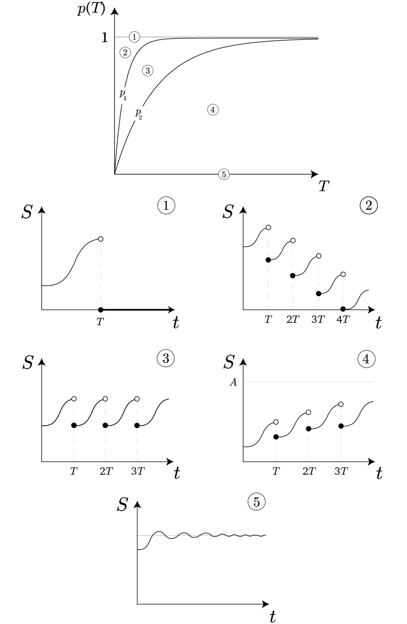
Figure 2. Bifurcation diagram $(T,p)$ associated to (8). In ①, all solutions converge to $(0,0)$; in ②, all solutions converge to $(0,0)$; in ③, almost all solutions tend towards the disease-free (non-trivial) periodic solution $(\mathcal{S},0)$; in ④, almost all solutions tend towards the endemic periodic solution $(\mathcal{S},\mathcal{I})$; in ⑤, almost all solutions tend towards the endemic equilibrium $(\mathcal{S},\mathcal{I})$. Compare with the numerical simulation of these five scenarios in Figure 9.

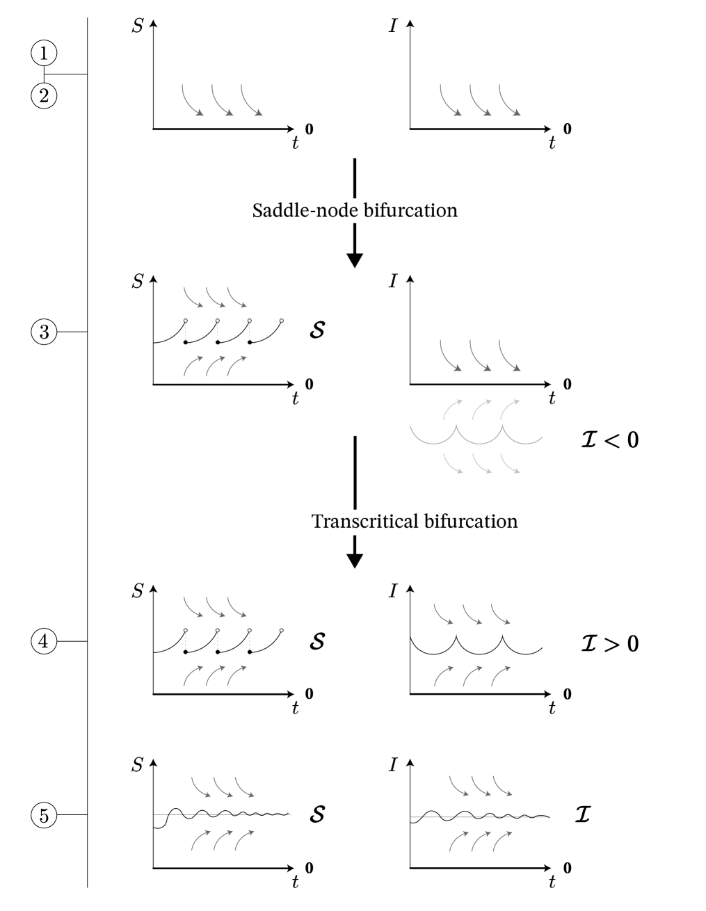
Figure 3. Bifurcations associated to the diagram $(T,p)$ associated to (8). From ② to ③: saddle-node associated to the solution $(0,0)$; From ③ to ④: transcritical bifurcation associated to $(\mathcal{S},0)$. For the numeration ① to ⑤, see Theorem A and Figure 2.

Items of Theorem A	Reference / Section
(1)	Trivial
(2)	Section 8
(3)	Sections 7 and 9
(4)	Section 10
(5)	See reference [10]
(6)	Section 11
(7)	Section 6

Table 1. Structure of the proof of Theorem A and the location of the items throughout the present article.

3.5. Pulse vaccination and seasonality

Seasonal variations may be captured by introducing periodically-perturbed terms into a deterministic differential equation [14, 16]. The periodically-perturbed term $\Psi(t)$ in $\beta_{\gamma}(t)$ may be seen as a natural periodic map over time with two global extrema (governing the high and lower seasons defined by weather conditions). Corollary 1, proved in Section 13, confirms the numerical results suggested by Choisy et al. [40]: neglecting the effect of the amplitude of the seasonal transmission can lead to somewhat overoptimistic values of the optimal pulse period.

Corollary 1.

For $\gamma,\omega>0$ small and $A>S_{c}$, the $T$-periodic solution $(\mathcal{S},0)$ is asymptotically stable if and only if $p_{2}^{\text{seas}}(T)<p<p_{1}(T)$ where

$$p_{1}(T)=1-e^{-AT}\quad\text{and}\quad{p_{2}^{\text{seas}}(T)=1-e^{-\left[(A-S_{c})T+\gamma\displaystyle\int_{0}^{T}\Psi(\omega t)\mathcal{S}(t)\,\mathrm{d}t\right]}}.$$

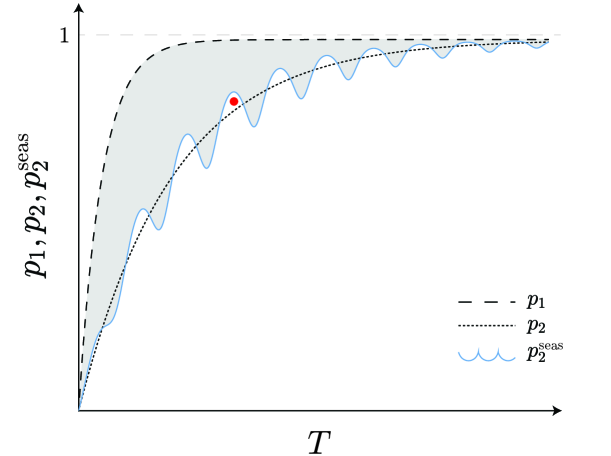
Figure 4. Illustration of Corollary 1: the $T$-periodic solution $(\mathcal{S},0)$ is asymptotically stable if and only if $p_{2}^{\text{seas}}(T)<p<p_{1}(T)$. The red dot corresponds to a point in the bifurcation diagram where $(\mathcal{S},0)$ is stable (without seasonality) and unstable (with seasonality).

One aspect that contributes to the complexity of (8) is the existence of chaos. Let $\mathcal{U}\subset\Omega$ such that $0<p<p_{2}(T)$ ($\Rightarrow\mathcal{R}_{p}>1$). Under the condition that $T=k\tau/\omega$, $k\in{\mathbb{N}}$, there is an endemic $T$-periodic solution for (8) (see Item (5) of Theorem A). In what follows, we assume that $M$ is diffeomorphic to a circloid.

Definition 4.

An embedding $F:M\rightarrow M$ is said to have a horseshoe if for some $N,n\in{\mathbb{N}}$, the map $F^{N}$ has a uniformly hyperbolic invariant set $\Upsilon\subset M$ such that $F^{N}|_{\Upsilon}$ is topologically conjugate to the full shift on $n$ symbols $(\Sigma_{n},\sigma)$ where $\sigma$ is the usual shift operator.

A vector field possesses a (suspended) horseshoe if the first return map to a cross-section does. The existence of a horseshoe for the embedding $F$ is equivalent to the notion of topological chaos ($\Leftrightarrow$ $F$ has positive topological entropy).

Theorem B.

For $0<p<p_{2}(T)$, $T=k\tau/\omega$, $k\in{\mathbb{N}}$ and $\omega\in\mathbb{R}^{+}$, if $\gamma$ is sufficiently large then ${f}_{\gamma}$ has a (suspended) topological horseshoe.

The shift dynamics obtained for (4) differ from those considered in [45], as discussed in Section 16. The proof of Theorem B is performed in Section 14.

3.6. Biological consequences

As suggested by Theorem A, the global eradication of an epidemic by means of pulse vaccination is always possible, provided the vaccination coverage is large enough.

Based on experimental data, the World Health Organization recommends that the time between successive pulses should be as short as possible. For a specific vaccination coverage $p\in(0,1)$, there exists a pulse interval $(0,T_{2})$ where $T_{2}=\dfrac{\left|\ln{(1-p)}\right|}{A-S_{c}}$ that ensures the effective implementation of this campaign ($\Leftrightarrow\mathcal{R}_{p}<1$); that is, the $T$-periodic administration of doses with $T\in(0,T_{2})$ leads to the global eradication of the disease, and $T_{2}$ is the optimal time that determines the fastest eradication. For a specific vaccination coverage $p>0$, if $T>T_{2}$ then $\mathcal{R}_{p}>1$.

Adding seasonality to our model, the epidemic threshold $S_{c}$ also depends on $\beta_{\gamma}$. Corollary 1 stresses that neglecting the effect of the amplitude of the seasonal transmission can lead to overoptimistic values of the optimal pulse period $T_{2}$. It also stresses that the best moment for vaccination corresponds to the local minimizers of $\beta_{\gamma}$. Theorem B says that the number of Susceptible individuals and Infectious in the presence of seasonal variations could be unpredictable.

4. Preparatory section

In this section, we collect useful lemmas needed for the proof of Theorems  A, B and Corollary 1. We start by proving the existence of a compact region where the dynamics lies.

Lemma 1.

The region defined by

$$\mathcal{M}=\left\{(S,I)\in(\mathbb{R}_{0}^{+})^{2}:\quad 0\leq S\leq A,\quad 0\leq S+I\leq\dfrac{A(\sigma+g+A)}{\sigma+g},\quad S,I\geq 0\right\}$$

is positively flow-invariant for (8).

Proof.

We can easily to check that $(\mathbb{R}_{0}^{+})^{2}$ is flow-invariant. Now, we show that if $(S_{0},I_{0})\in\mathcal{M}$, then $\varphi_{0}\left(t,(S_{0},I_{0})\right)$, $t\in\mathbb{R}_{0}^{+}$, is contained in $\mathcal{M}$. Let us define

$$\nu(t)=S(t)+I(t)\geq 0$$

associated to the trajectory $\varphi_{0}\left(t,(S_{0},I_{0})\right)$. Omitting the variables’ dependence on $t$, one knows that

$$\begin{array}[]{lcl}\dot{\nu}&=&\dot{S}+\dot{I}\\ \\ &=&S(A-S)-\beta_{0}IS+\beta_{0}IS-(\sigma+g)I\\ \\ &=&S(A-S)-(\sigma+g)I,\\ \end{array}$$

from which we deduce that

$$\begin{array}[]{lcl}\dot{\nu}+(\sigma+g)\nu&=&S(A-S)-(\sigma+g)I+(\sigma+g)S+(\sigma+g)I\\ \\ &=&S(A-S)+(\sigma+g)S\\ \\ &\leq&(\sigma+g+A)S.\\ \end{array}$$

If $\beta_{0}=p=0$, the first component of equation (8) would represent logistic growth. Thus, its solution would have an upper bound of $A$ (by (C2)). This property is also verified for $\beta_{0},p\in\mathbb{R}^{+}$, even if $p$ is applied periodically (note that $p\in[0,1]$). In particular, we have

$$\begin{array}[]{lcl}\dot{\nu}+(\sigma+g)\nu\leq(\sigma+g+A)A.\end{array}$$

The classical differential version of the Gronwall’s Lemma says that for all $t\in\mathbb{R}^{+}_{0}$, we have

$$\nu(t)\leq\nu_{0}e^{-(\sigma+g)t}-\frac{(\sigma+g+A)A}{(\sigma+g)}\left(e^{-(\sigma+g)t}-1\right),$$

where $\nu(0)\coloneqq\nu_{0}=S(0)+I(0)\geq 0$. Taking the limit when $t\rightarrow+\infty$, we get:

$$0\leq\lim_{t\rightarrow+\infty}\nu(t) \leq \lim_{t\rightarrow+\infty}\left[\nu_{0}e^{-(\sigma+g)t}-\frac{(\sigma+g+A)A}{(\sigma+g)}\left(e^{-(\sigma+g)t}-1\right)\right]$$

$$= \frac{(\sigma+g+A)A}{(\sigma+g)}.$$

Since $\displaystyle\lim_{t\rightarrow+\infty}\nu(t)=\displaystyle\lim_{t\rightarrow+\infty}\left(S(t)+I(t)\right)$, the result is proved. ∎

In the following result, let $D$ be an open subinterval of $\mathbb{R}^{+}_{0}$.

Lemma 2.

With respect to (8), the following assertions hold $p\geq 0$:

1. $S(t)<S_{c}$ for all $t\in D$ if and only if $I$ is decreasing in $D$;

2. $S(t)=S_{c}$ for all $t\in D$ if and only if $I$ is constant;

3. $S(t)>S_{c}$ for all $t\in D$ if and only if $I$ is increasing in $D$.

Proof.

We just show (1). The proof of (2) and (3) follows from the same reasoning. We know that the Infectious is decreasing if and only if $\dot{I}(t)<0$, where $t\in D$. Indeed,

$$\dot{I}(t)<0$$

$$\overset{\eqref{modelo3}}{\Leftrightarrow} \beta_{0}S(t)I(t)-\left(\sigma+g\right)I(t)<0$$

$$\Leftrightarrow \beta_{0}S(t)<\sigma+g$$

$$\Leftrightarrow S(t)<\dfrac{\sigma+g}{\beta_{0}}=S_{c},$$ (11)

and the result is proved. ∎

Remark.

The constant $S_{c}$ defined in (10) will be called the epidemic threshold and is the critical limit of the Susceptible individuals that defines whether the epidemic spreads or not [13]. When $\gamma=0$, the most intriguing dynamical scenario is when $S(t)-S_{c}$ takes different signs in $D\subset\mathbb{R}_{0}^{+}$ (See Figure 5).

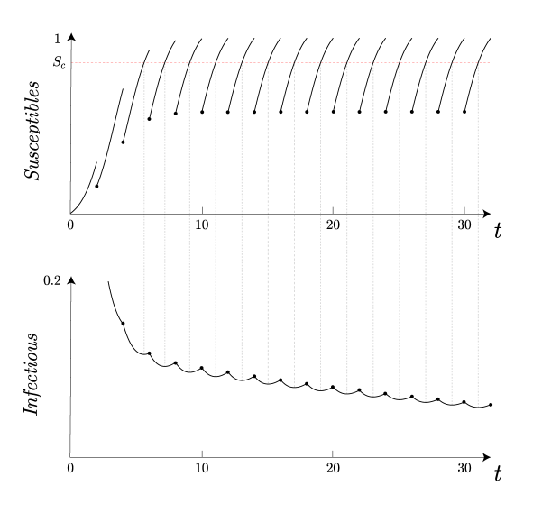
Figure 5. Illustration of Lemma 2 for $D=\mathbb{R}^{+}$: evolution of $S$ and $I$ as $t\in\mathbb{R}^{+}$ evolves.

Lemma 3.

With respect to (8), the following equivalence holds:

$$A>S_{c}\quad\Leftrightarrow\quad\mathcal{R}_{0}>1.$$

Proof.

The proof follows from simple calculations:

$$A>S_{c}\qquad\overset{\eqref{S_c(def)}}{\Leftrightarrow}\qquad A>\dfrac{\sigma+g}{\beta_{0}}\qquad\Leftrightarrow\qquad\dfrac{A\beta_{0}}{\sigma+g}>1\qquad\overset{\eqref{R0}}{\Leftrightarrow}\qquad\mathcal{R}_{0}>1.$$

∎

5. Stroboscopic maps and their fixed points

In this section, we study the existence of fixed points associated with the stroboscopic maps (time $T>0$) of the Susceptible and Infectious for system (8). We also analyze their stability in the sense of Subsection 2.2. For $n\in{\mathbb{N}}$ and $T>0$, using (9), define the sequences:

$$S_{n}=S\left(nT,(S_{0},I_{0})\right)\quad\text{and}\quad I_{n}=I\left(nT,(S_{0},I_{0})\right),$$

which may be seen as the stroboscopic $T$-maps associated to the trajectory of $(S_{0},I_{0})\in(\mathbb{R}_{0}^{+})^{2}$.

Lemma 4.

With respect to (8), the following assertions hold:

1. There exists $F_{I}:\mathbb{R}_{0}^{+}\rightarrow\mathbb{R}^{+}_{0}$ such that $I_{n+1}=F_{I}(I_{n})$ and

   $$F_{I}(y)=y\exp{\left\{\beta_{0}\displaystyle\int_{nT}^{(n+1)T}S(t)\,\mathrm{d}t\right\}}e^{-\left(\sigma+g\right)T};$$

2. The fixed point of $F_{I}$ is:

   1. $y=0$ if  $\displaystyle\dfrac{1}{T}\int_{0}^{T}\mathcal{S}(t)\,\mathrm{d}t\neq S_{c}$;

   2. (any) $y\in\mathbb{R}_{0}^{+}$ if  $\displaystyle\dfrac{1}{T}\int_{0}^{T}\mathcal{S}(t)\,\mathrm{d}t=S_{c}$.

Proof.

1. From (8), for $I(t)>0$ for all $t\in\mathbb{R}_{0}^{+}$, we have

   $$\dot{I}(t)=\beta_{0}S(t)I(t)-(\sigma+g)I(t)$$

   $$\Rightarrow \displaystyle\int_{t_{0}}^{t}\dfrac{\mathrm{d}I(\tau)}{I(\tau)}=\beta_{0}\displaystyle\int_{t_{0}}^{t}S(\tau)\mathrm{d}\tau-(m+g)\displaystyle\int_{t_{0}}^{t}\,\mathrm{d}\tau$$

   $$\Leftrightarrow \ln{I(t)}-\ln{I(t_{0})}=\beta_{0}\displaystyle\int_{t_{0}}^{t}S(\tau)\,\mathrm{d}\tau-(m+g)(t-t_{0})$$

   $$\Leftrightarrow I(t)=I_{0}\exp{\left\{\beta_{0}\displaystyle\int_{t_{0}}^{t}S(\tau)\,\mathrm{d}\tau\right\}}e^{-\left(\sigma+g\right)\left(t-t_{0}\right)},$$

   where $I(t_{0})\coloneqq I_{0}>0$. The sequence $I_{n+1}=I\left((n+1)T,(S_{0},I_{0})\right)$ is then computed as

   $$I_{n+1}\coloneqq I_{n}\exp{\left\{\beta_{0}\displaystyle\int_{nT}^{(n+1)T}S(t)\,\mathrm{d}t\right\}}e^{-\left(\sigma+g\right)T}$$

   $$\Leftrightarrow I_{n+1}=F_{I}(I_{n}),$$

   where $F_{I}(y)=y\exp{\left\{\beta_{0}\displaystyle\int_{nT}^{(n+1)T}S(t)\,\mathrm{d}t\right\}}e^{-\left(\sigma+g\right)T}$.

2. The fixed points of $F_{I}$ can be found by solving the equation $F_{I}(y^{\star})=y^{\star}$ which is equivalent to

   $$y^{\star}\exp{\left\{\beta_{0}\displaystyle\int_{nT}^{(n+1)T}S(t)\,\mathrm{d}t\right\}}e^{-\left(\sigma+g\right)T}=y^{\star}$$

   $$\Leftrightarrow y^{\star}\exp\left(\displaystyle\dfrac{1}{T}\int_{0}^{T}\mathcal{S}(t)\,\mathrm{d}t-S_{c}\right)=y^{\star}.$$

   In other words, if  $\displaystyle\dfrac{1}{T}\int_{0}^{T}\mathcal{S}(t)\,\mathrm{d}t\neq S_{c}$, then the fixed point of $F_{I}$ is given by $y^{\star}=0$. Otherwise any $y\in\mathbb{R}_{0}^{+}$ is a solution of $F_{I}(y)=y$.

∎

If  $\displaystyle\dfrac{1}{T}\int_{0}^{T}\mathcal{S}(t)\,\mathrm{d}t\neq S_{c}$, then the unique fixed point of $F_{I}$ is $y^{\star}=0$. Therefore, we focus the analysis on this fixed point. We remind the definition of $p_{1}$ from the statement of Theorem A: $p_{1}\equiv p_{1}(T)=1-e^{-AT}$, $T>0$.

Lemma 5.

With respect to (8), the following assertions hold when $I=0$:

1. There exists $F_{S}:\mathbb{R}_{0}^{+}\rightarrow\mathbb{R}_{0}^{+}$ such that $S_{n+1}=F_{S}(S_{n})$ and

   $$F_{S}(x)=\displaystyle\dfrac{A\,x\left(1-p\right)e^{AT}}{x\left(e^{AT}-1\right)+A};$$

2. The map $F_{S}(x)$ has two fixed points:

   $$x_{1}^{\star}=A\left(1-\dfrac{pe^{AT}}{e^{AT}-1}\right)\quad\text{and}\quad x_{2}^{\star}=0.$$

   For $T>0$, if $p>p_{1}(T)$, then $x_{1}^{\star}<0$.

Proof.

1. We study system (8) assuming $I=0$ (the unique fixed point of $F_{I}$ if $\displaystyle\dfrac{1}{T}\int_{0}^{T}\mathcal{S}(t)\,\mathrm{d}t\neq S_{c}$ (cf. Lemma 4). The growth of $S$ for $t_{0}=nT\leq t<(n+1)T$ is given by

   $$\begin{cases}\vskip 6.0pt plus 2.0pt minus 2.0pt&\dot{S}(t)=S(t)\left(A-S(t)\right)\,\,\,\,\,\,\,,\quad\,t\neq nT\\ &S(nT)=(1-p)S(nT^{-})\,\,\,,\quad\,t=nT.\end{cases}$$ (12)

   Integrating (12) between pulses, and assuming that $S(t)(A-S(t))$ does not vanish, we obtain

   $$\dot{S}(t)=S(t)\left(A-S(t)\right)$$

   $$\Leftrightarrow \displaystyle\int_{t_{0}}^{t}\dfrac{\mathrm{d}S(\tau)}{S(\tau)\left(A-S(\tau)\right)}=\displaystyle\int_{t_{0}}^{t}\,\mathrm{d}\tau$$

   $$\Leftrightarrow \displaystyle\int_{t_{0}}^{t}\dfrac{\mathrm{d}S(\tau)}{S(\tau)\left(A-S(\tau)\right)}=t-t_{0}.$$ (13)

   
   

   From (13) we get the following explicit expression for $S(t)$:

   $$S(t)=\displaystyle\dfrac{A\,S_{0}}{S_{0}+\left(A-S_{0}\right)e^{-A\left(t-t_{0}\right)}}\quad,\qquad t\geq t_{0}\geq 0,$$ (14)

   where $S(t_{0})\coloneqq S_{0}$ and $A>S_{0}$. Notice that (14) holds between pulses. Now, we find a general expression that gives the number of the Susceptible between two consecutive vaccination shots, $nT$ and $(n+1)T$, bearing in mind that

   $$S(nT^{-})=\displaystyle\lim_{t\rightarrow nT^{-}}S(t)\,\,,\quad S(nT)=(1-p)S(nT^{-})\,\,,\quad n\in\mathbb{N}.$$ (15)

   Indeed, for $0\leq t<T$ (no vaccination yet), we get

   $$S(t)=\displaystyle\dfrac{A\,S(0)}{S(0)+\left(A-S(0)\right)e^{-At}}$$

   and for $T\leq t<2T$, one may write

   $$S(t)=\displaystyle\dfrac{A\left(1-p\right)S(T^{-})}{\left(1-p\right)S(T^{-})+\left[A-(1-p)S(T^{-})\right]e^{-A\left(t-T\right)}}$$

   Analogously, for $2T\leq t<3T$, one has

   $$S(t)=\displaystyle\dfrac{A\left(1-p\right)S(2T^{-})}{\left(1-p\right)S(2T^{-})+\left[A-\left(1-p\right)S(2T^{-})\right]e^{-A\left(t-2T\right)}}.$$

   By induction over $n\in{\mathbb{N}}$, for $nT\leq t<(n+1)T$, it is easy to show that the general expression for $S(t)$ is given by

   $$S(t)=\displaystyle\dfrac{A\left(1-p\right)S(nT^{-})}{\left(1-p\right)S(nT^{-})+\left[A-\left(1-p\right)S(nT^{-})\right]e^{-A\left(t-nT\right)}}.$$

   Using (15) and considering $S_{n}=S\left(nT,(S_{0},I_{0})\right)$ we get

   $$S(t)=\displaystyle\dfrac{A\,S_{n}}{S_{n}+\left(A-S_{n}\right)e^{-A\left(t-nT\right)}}\quad,$$ (16)

   where $nT\leq t<(n+1)T$. In particular, this leads to

   $$S((n+1)T^{-})=\displaystyle\dfrac{A\left(1-p\right)S(nT^{-})}{\left(1-p\right)S(nT^{-})+\left[A-\left(1-p\right)S(nT^{-})\right]e^{-AT}}$$

   $$\overset{\eqref{notions}}{\Leftrightarrow} \dfrac{S((n+1)T)}{1-p}=\displaystyle\dfrac{A\left(1-p\right)S(nT^{-})}{\left(1-p\right)S(nT^{-})+\left[A-\left(1-p\right)S(nT^{-})\right]e^{-AT}}$$

   $$\Leftrightarrow S_{n+1}=\displaystyle\dfrac{A\,S_{n}\left(1-p\right)}{S_{n}+\left(A-S_{n}\right)e^{-AT}}$$

   $$\Leftrightarrow S_{n+1}=\displaystyle\dfrac{A\,S_{n}\left(1-p\right)}{S_{n}\left(1-e^{-AT}\right)+Ae^{-AT}}.$$ (17)

   Multiplying both the numerator and the denominator of (17) by $e^{AT}>0$, we get

   $$S_{n+1}\coloneqq\displaystyle\dfrac{A\,S_{n}\left(1-p\right)e^{AT}}{S_{n}\left(e^{AT}-1\right)+A}\qquad\Leftrightarrow\qquad S_{n+1}=F_{S}(S_{n}),$$

   where

   $$F_{S}(x)=\displaystyle\dfrac{A\,x\left(1-p\right)e^{AT}}{x\left(e^{AT}-1\right)+A}.$$

2. Let $x^{\star}$ be a fixed point of $F$, i.e. $F_{S}(x^{\star})=x^{\star}.$ Then

   $$\displaystyle\dfrac{A\,x^{\star}\left(1-p\right)e^{AT}}{x^{\star}\left(e^{AT}-1\right)+A}=x^{\star}$$

   $$\Leftrightarrow \displaystyle\dfrac{A\,\left(1-p\right)e^{AT}}{x^{\star}\left(e^{AT}-1\right)+A}=1\qquad\qquad\qquad\qquad\quad\,\vee\quad x^{\star}=0$$

   $$\Leftrightarrow A\left(1-p\right)e^{AT}=x^{\star}\left(e^{AT}-1\right)+A\qquad\qquad\vee\quad x^{\star}=0$$

   $$\Leftrightarrow x^{\star}\left(e^{AT}-1\right)=A\left(e^{AT}-1\right)-Ape^{AT}\quad\quad\,\,\vee\quad x^{\star}=0$$

   $$\Leftrightarrow x^{\star}=A\left(1-\dfrac{pe^{AT}}{e^{AT}-1}\right)\qquad\qquad\qquad\qquad\,\,\,\vee\quad x^{\star}=0.$$

   Hence $F_{S}$ has two fixed points:

   $$x_{1}^{\star} = A\left(1-\dfrac{pe^{AT}}{e^{AT}-1}\right)$$

   $$x_{2}^{\star} = 0,$$

   where $x_{1}^{\star}>0$ if and only if

   $$A\left(1-\dfrac{pe^{AT}}{e^{AT}-1}\right)>0\quad\Leftrightarrow\quad 1-\dfrac{pe^{AT}}{e^{AT}-1}>0\quad\Leftrightarrow\quad p<1-e^{-AT}\quad\Leftrightarrow\quad p<p_{1}(T).$$

∎

Combining Lemmas 4 and 5, we know that if  $\displaystyle\dfrac{1}{T}\int_{0}^{T}\mathcal{S}(t)\,\mathrm{d}t\neq S_{c}$, then $(F_{S},F_{I})$ has two fixed non-negative points: $(0,0)$ and $(x_{1}^{\star},0)$. In the flow of (8), they are denoted by $(0,0)$ (stationary trivial equilibrium) and $(\mathcal{S},0)$ (periodic non-trivial disease solution).

Lemma 6.

For $T>0$, the non-trivial $T$-periodic solution of (8) associated to $(x_{1}^{\star},0)$ is parametrised by

$$(\mathcal{S}(t),0)=\left(\dfrac{A\left[e^{AT}\left(1-p\right)-1\right]}{e^{AT}\left(1-p\right)-1+pe^{A\left(T-(t-t_{0})\right)}},0\right),$$

where $t_{0}=nT\leq t<(n+1)T$ and $n\in{\mathbb{N}}$.

Remark.

The expression of $(\mathcal{S}(t),0)$ does not depend on the transmission rate $\beta$.

Proof.

Replacing $S_{0}$ by $x_{1}^{\star}$ in (14), we obtain

$$\mathcal{S}(t) = \displaystyle\dfrac{A\,x_{1}^{\star}}{x_{1}^{\star}+\left(A-x_{1}^{\star}\right)e^{-A(t-t_{0})}}$$ (18)

$$= \displaystyle\dfrac{A^{2}\left(1-\dfrac{pe^{AT}}{e^{AT}-1}\right)}{A\left(1-\dfrac{pe^{AT}}{e^{AT}-1}\right)+\left(A-A\left(1-\dfrac{pe^{AT}}{e^{AT}-1}\right)\right)e^{-A(t-t_{0})}}$$

$$= \displaystyle\dfrac{A\left[\dfrac{e^{AT}-1-pe^{AT}}{e^{AT}-1}\right]}{\dfrac{e^{AT}-1-pe^{AT}+pe^{AT}e^{-A(t-t_{0})}}{e^{AT}-1}}$$

$$= \displaystyle\dfrac{A\left[e^{AT}\left(1-p\right)-1\right]}{e^{AT}\left(1-p\right)-1+pe^{A\left(T-(t-t_{0})\right)}},$$

where $t_{0}=nT\leq t<(n+1)T$ and $n\in{\mathbb{N}}$. By construction, this solution is $T$-periodic (a consequence of Lemmas 4 and 5). ∎

6. Basic reproduction number $\mathcal{R}_{p}$ for (8)

For $T>0$, following [15, Eq. (3.15)], we may define the basic reproduction number $\mathcal{R}_{p}$ in the absence of seasonality for system (8) as

$$\mathcal{R}_{p}(T):=\displaystyle\dfrac{\beta_{0}}{\sigma+g}\dfrac{1}{T}\int_{0}^{T}\mathcal{S}(t)\,\mathrm{d}t=\dfrac{1}{S_{c}T}\int_{0}^{T}\mathcal{S}(t)\,\mathrm{d}t,$$ (19)

based on the disease-free periodic solution $\mathcal{S}(t)$ given explicitly in Lemma 6. The quantity $\mathcal{R}_{p}$ (when less than 1) can be used to measure the velocity at which the disease is eradicated. For clarity, we omit the dependence of $\mathcal{R}_{p}$ on $T>0$. In the sequel, we present a series of properties of $\mathcal{R}_{p}$.

Lemma 7.

With respect to (8), the following assertions hold for $p\in[0,1)$ and $T>0$:

1. $\mathcal{R}_{p}=\displaystyle\mathcal{R}_{0}\left[\dfrac{\ln{(1-p)}}{AT}+1\right]$;

2. if $\mathcal{R}_{p}=1$, then $F_{I}$ has infinitely many fixed points;

3. for $T>0$ and $p>0$, we have $\frac{\partial\mathcal{R}_{p}}{\partial T}(T)>0$ and  $\frac{\partial\mathcal{R}_{p}}{\partial p}(T)<0$;

4. $\displaystyle\lim_{T\rightarrow+\infty}\mathcal{R}_{p}=\mathcal{R}_{0}$();

5. If $p=0$, then $\mathcal{R}_{p}=\mathcal{R}_{0}$.
   

Proof.

1. For the sake of simplicity, let us assume $t_{0}=0$. Then we have

   $$\int_{0}^{T}\mathcal{S}(t)\,\mathrm{d}t\overset{\eqref{S_infect_free}}{=}\int_{0}^{T}\dfrac{A\left[e^{AT}\left(1-p\right)-1\right]}{e^{AT}\left(1-p\right)-1+pe^{A\left(T-t\right)}}\,\mathrm{d}t.$$

   Using Maple, we get

   $$\int_{0}^{T}\mathcal{S}(t)\,\mathrm{d}t=\ln{\left(1-p\right)}+AT$$ (20)

   and then:

   $$\mathcal{R}_{p} = \displaystyle\dfrac{\beta_{0}}{\sigma+g}\dfrac{1}{T}\int_{0}^{T}\mathcal{S}(t)\,\mathrm{d}t$$

   $$\overset{\eqref{integral_S_til}}{=} \dfrac{\beta_{0}}{\sigma+g}\dfrac{1}{T}\big{[}\ln{(1-p)}+AT\big{]}$$

   $$\overset{\eqref{R0Sc}}{=} \dfrac{1}{S_{c}T}\big{[}\ln{(1-p)}+AT\big{]}$$

   $$\overset{\eqref{R0},\eqref{R0Sc}}{=} \displaystyle\mathcal{R}_{0}\left[\dfrac{\ln{(1-p)}}{AT}+1\right].$$

2. Using the following chain of equivalences:

   $$\mathcal{R}_{p}=1 \Leftrightarrow \displaystyle\dfrac{1}{T}\int_{0}^{T}\mathcal{S}(t)\,\mathrm{d}t=S_{c}$$

   $$\Leftrightarrow \exp{\left\{\beta_{0}\displaystyle\int_{nT}^{(n+1)T}\mathcal{S}(t)\,\mathrm{d}t\right\}}e^{-\left(\sigma+g\right)T}=1,$$

   the result follows by observing the analytic expression of $F_{I}$ in Lemma 4.

3. From the proof of item (1), one knows that $\mathcal{R}_{p}=\mathcal{R}_{0}\left[\frac{\ln{(1-p)}}{AT}+1\right]$. If $p>0$, then

   $$\frac{\partial\mathcal{R}_{p}}{\partial T}(T)=-\dfrac{\mathcal{R}_{0}\ln{\left(1-p\right)}}{AT^{2}}>0\qquad\text{and}\qquad\frac{\partial\mathcal{R}_{p}}{\partial p}(T)=-\dfrac{\mathcal{R}_{0}}{AT\left(1-p\right)}<0.$$

Items (4) and (5) are straightforward using the formula of $\mathcal{R}_{p}$ of item (1). ∎

The following useful result relates the stability of the impulsive periodic solution of Lemma 6 with the basic reproduction number $\mathcal{R}_{p}$ for (8).

Lemma 8.

With respect to system (8), if  $A>S_{c}$ (), then  $\mathcal{R}_{p}<1\,\,\Leftrightarrow\,\,p>p_{2}.$

Proof.

The proof follows from the following chain of equivalences:

$$\mathcal{R}_{p}<1$$

$$\Leftrightarrow \dfrac{1}{S_{c}T}\big{[}\ln{(1-p)}+AT\big{]}<1$$

$$\Leftrightarrow \big{[}\ln{(1-p)}+AT\big{]}<S_{c}T$$

$$\Leftrightarrow 1-p<e^{(S_{c}-A)T}$$

$$\Leftrightarrow p>1-e^{-(A-S_{c})T}$$

$$\Leftrightarrow p>p_{2}.$$

∎

7. Local stability of the disease-free solutions

The next result proves the local asymptotic stability of the disease-free periodic solutions of (8) using Floquet multipliers, say $(0,0)$ and $(\mathcal{S},0)$.

Proposition 3.

With respect to (8), the following assertions hold for $T>0$:

1. the disease-free trivial solution $(0,0)$ is locally asymptotically stable provided $p>p_{1}(T)$;

2. the disease-free periodic solution $(\mathcal{S},0)$ is locally asymptotically stable provided $p_{2}(T)<p<p_{1}(T)$.

Proof.

The stability of the disease-free periodic solution is found by analyzing the behavior of initial conditions close to it. This is achievable by computing the monodromy matrix (see [31, Chapter II, pp. 28]). If the absolute value of the eigenvalues (Floquet multipliers) of the monodromy matrix is less than one, then the periodic solution $(\mathcal{S},0)$ is asymptotically stable [31, Theorem 3.5, pp. 30].

We exhibit the computations near the $T$-periodic solution $(\mathcal{S},0)$. For $t\geq 0$, we set

$$S(t) = \mathcal{S}(t)+s(t)$$

$$I(t) = \mathcal{I}(t)+i(t)\quad\Leftrightarrow\quad I(t)\,\,\,\,=\,\,\,\,i(t),$$

where $s(t)$ and $i(t)$ are small terms close to 0. We will show that they vanish when $t$ increases. Omitting the dependence of the variables on $t$, from (8) and (7), one may write

$$\dfrac{\mathrm{d}s}{\mathrm{d}t} = \dfrac{\mathrm{d}S}{\mathrm{d}t}-\dfrac{\mathrm{d}\mathcal{S}}{\mathrm{d}t}$$

$$= S(A-S)-\beta_{0}SI-\big{[}\mathcal{S}(A-\mathcal{S})-\beta_{0}\mathcal{S}\mathcal{I}\big{]}$$

$$\overset{\mathcal{I}=0}{=} SA-S^{2}-\beta_{0}SI-\mathcal{S}A+\mathcal{S}^{2}$$

$$= -\mathcal{S}A+\mathcal{S}^{2}+A(\mathcal{S}+s)-(\mathcal{S}+s)^{2}-\beta_{0}(\mathcal{S}+s)i$$

$$= -\mathcal{S}A+\mathcal{S}^{2}+\mathcal{S}A+sA-\mathcal{S}^{2}-2s\mathcal{S}-s^{2}-\beta_{0}\mathcal{S}i-\beta_{0}si$$

$$= As-2s\mathcal{S}-\beta_{0}\mathcal{S}i-\beta_{0}si-s^{2}$$

$$= (A-2\mathcal{S}-\beta_{0}i)s-\beta_{0}\mathcal{S}i-s^{2}$$

and

$$\dfrac{\mathrm{d}i}{\mathrm{d}t} = \dfrac{\mathrm{d}I}{\mathrm{d}t}-\dfrac{\mathrm{d}\mathcal{I}}{\mathrm{d}t}$$

$$= \dfrac{\mathrm{d}I}{\mathrm{d}t}$$

$$= \beta_{0}\mathcal{S}i-(\sigma+g)i$$

$$= \big{[}\beta_{0}\mathcal{S}-(\sigma+g)\big{]}i.$$

Hence, we model the evolution of $(s,i)$ as

$$\begin{array}[]{lcl}\begin{cases}\vskip 12.0pt plus 4.0pt minus 4.0pt&\dfrac{\mathrm{d}s}{\mathrm{d}t}=(A-2\mathcal{S}-\beta_{0}i)s-\beta_{0}\mathcal{S}i\\ \vskip 12.0pt plus 4.0pt minus 4.0pt\vskip 12.0pt plus 4.0pt minus 4.0pt&\dfrac{\mathrm{d}i}{\mathrm{d}t}=\big{[}\beta_{0}\mathcal{S}-(\sigma+g)\big{]}i\,,\qquad\qquad\qquad\qquad t\neq nT,\\ \vskip 6.0pt plus 2.0pt minus 2.0pt&s(nT)=(1-p)s(nT^{-})\\ \vskip 6.0pt plus 2.0pt minus 2.0pt&i(nT)=i(nT^{-})\,,\,\,\,\,\,\qquad\qquad\qquad\qquad\qquad t=nT.\end{cases}\end{array}$$ (23)

Note that $\mathcal{S}(t)$ is known explicitly (Lemma 6) and may be written as the periodic coefficient of $s(t)$ and $i(t)$. Lyapunov’s theory neglects quadratic terms to compute the stability of hyperbolic fixed points [42, §I6, p. 6]. The solutions of (23) may be written as

$$\begin{array}[]{lcl}\left(\begin{array}[]{c}s(t)\\ \\ i(t)\end{array}\right)=\Phi(t)\left(\begin{array}[]{c}s(0)\\ \\ i(0)\end{array}\right),\end{array}$$

where

$$\begin{array}[]{lcl}\Phi(t)=\left(\begin{array}[]{cc}\varphi_{1,1}(t)&\varphi_{1,2}(t)\\ \\ \varphi_{2,1}(t)&\varphi_{2,2}(t)\end{array}\right)\end{array}$$

is the fundamental matrix whose columns are the components of linearly independent solutions of (23), and $\Phi(0)$ is the identity matrix. According to Floquet theory [42, §VII.6.2, p. 146], $\Phi(t)$ satisfies

$$\begin{array}[]{lcl}\dfrac{\mathrm{d}\Phi}{\mathrm{d}t}\Big{|}_{(s^{\star},i^{\star})}&=&\mathcal{J}(t)\Phi(t)\\ \\ &=&\left(\begin{array}[]{cc}A-2\mathcal{S}(t)-\beta_{0}i^{\star}&-\beta_{0}s^{\star}-\beta_{0}\mathcal{S}(t)\\ \\ \\ 0&\beta_{0}\mathcal{S}(t)-\left(\sigma+g\right)\end{array}\right)\Phi(t)\\ \\ \\ &\overset{(s^{\star},i^{\star})\,=\,(0,0)}{=}&\left(\begin{array}[]{cc}A-2\mathcal{S}(t)&-\beta_{0}\mathcal{S}(t)\\ \\ \\ 0&\beta_{0}\mathcal{S}(t)-\left(\sigma+g\right)\end{array}\right)\Phi(t),\end{array}$$

where $\mathcal{J}(t)$ is the Jacobian matrix of (23) around the equilibrium point $(s^{\star},i^{\star})=(0,0)$. The fundamental matrix $\Phi(t)$ may be written as

$$\Phi(t) = \left(\begin{array}[]{cc}\exp{\left\{\displaystyle\int_{0}^{T}\left(A-2\mathcal{S}(t)\right)\,\mathrm{d}t\right\}}&\varphi_{1,2}(t)\\ \\ \\ 0&\exp{\left\{\displaystyle\int_{0}^{T}\left[\beta_{0}\mathcal{S}(t)-\left(\sigma+g\right)\right]\,\mathrm{d}t\right\}}\end{array}\right)$$

$$= \left(\begin{array}[]{cc}\exp{\left\{AT-2\displaystyle\int_{0}^{T}\mathcal{S}(t)\,\mathrm{d}t\right\}}&\varphi_{1,2}(t)\\ \\ \\ 0&\exp{\left\{\beta_{0}\displaystyle\int_{0}^{T}\mathcal{S}(t)\,\mathrm{d}t-\left(\sigma+g\right)T\right\}}\end{array}\right).$$

Computing the exact form of $\varphi_{1,2}(t)$ is not necessary since it is not needed in the subsequent analysis. Since the linearisation of the third and fourth equations of (23) results in

$$\begin{array}[]{lcl}\left(\begin{array}[]{c}s(nT)\\ \\ i(nT)\end{array}\right)=\left(\begin{array}[]{cc}1-p&0\\ \\ 0&1\end{array}\right)\left(\begin{array}[]{c}s(nT^{-})\\ \\ i(nT^{-})\end{array}\right),\end{array}$$

then the Floquet multipliers of $(\mathcal{S},0)$ are the roots of

$$\small\det{\left[\begin{array}[]{cc}(1-p)\,\exp{\left\{AT-2\displaystyle\int_{0}^{T}\mathcal{S}(t)\,\mathrm{d}t\right\}}-\lambda&\varphi_{1,2}(t)\\ \\ \\ 0&\exp{\left\{\beta_{0}\displaystyle\int_{0}^{T}\mathcal{S}(t)\,\mathrm{d}t-\left(\sigma+g\right)T\right\}}-\lambda\end{array}\right]} = 0.$$

They are given by

$$\lambda_{1} = (1-p)\,\exp{\left\{AT-2\displaystyle\int_{0}^{T}\mathcal{S}(t)\,\mathrm{d}t\right\}}>0$$ (29)

$$\lambda_{2} = \exp{\left\{\beta_{0}\displaystyle\int_{0}^{T}\mathcal{S}(t)\,\mathrm{d}t-\left(\sigma+g\right)T\right\}}>0$$ (30)

Floquet multipliers near $(\mathcal{S},0)$: From (29) we get

$$\lambda_{1}<1$$

$$\Leftrightarrow (1-p)\,\exp{\left\{AT-2\displaystyle\int_{0}^{T}\mathcal{S}(t)\,\mathrm{d}t\right\}}<1$$

$$\overset{\eqref{integral_S_til}}{\Leftrightarrow} (1-p)<\exp{\left\{-AT+2\ln{(1-p)}+2AT\right\}}$$

$$\Leftrightarrow \ln{(1-p)}+AT>0$$

$$\Leftrightarrow p<p_{1},$$

and from (30) we deduce that

$$\lambda_{2}<1$$

$$\Leftrightarrow \exp{\left\{\beta_{0}\displaystyle\int_{0}^{T}\mathcal{S}(t)\,\mathrm{d}t-\left(\sigma+g\right)T\right\}}<1$$

$$\Leftrightarrow \beta_{0}\displaystyle\int_{0}^{T}\mathcal{S}(t)\,\mathrm{d}t-\left(\sigma+g\right)T<0$$

$$\Leftrightarrow \dfrac{1}{T}\int_{0}^{T}\mathcal{S}(t)\,\mathrm{d}t<\dfrac{\sigma+g}{\beta_{0}}\overset{\eqref{R0Sc}}{=}S_{c}$$

$$\Leftrightarrow \dfrac{\beta_{0}}{\sigma+g}\frac{1}{T}\int_{0}^{T}\mathcal{S}(t)\,\mathrm{d}t<1$$

$$\overset{\eqref{RpAND_Sc}}{\Leftrightarrow} \mathcal{R}_{p}<1.$$

Floquet multipliers near $(0,0)$:

$$\lambda_{1} = (1-p)\,e^{AT}$$

$$\lambda_{2} = e^{-\left(\sigma+g\right)T}.$$

It is easy to check that $\lambda_{1}<1$ if and only if $p>p_{1}(T)$ and $\lambda_{2}<1$. The result is then shown. ∎

The maps $p_{1}$ and $p_{2}$ given in Theorem A admit inverse. Let us denote them by $T_{1}$ and $T_{2}$, respectively, which may be explicitly given by

$$T_{1}(p)\coloneqq\dfrac{\left|\ln{(1-p)}\right|}{A}\quad\text{and}\quad T_{\text{2}}(p)\coloneqq\dfrac{\left|\ln{(1-p)}\right|}{A-S_{c}}\,\,,\qquad\text{for}\,\,\,A>S_{c}.$$

Omitting the dependence of $T_{1}$ and $T_{2}$ on $p$, the following result is equivalent to Proposition 3 . It characterizes the stability of the stability of $(0,0)$ and $(\mathcal{S},0)$ as function of the variable $T$ (cf. Figure 2).

Corollary 2.

With respect to (8), the following assertions hold for $p>0$:

1. If  $T<T_{1}(p)$, then there are no non-trivial periodic solutions; the trivial equilibrium $(0,0)$ is stable;

2. If  $T_{1}(p)<T<T_{2}(p)$, then the disease-free periodic solution $(\mathcal{S},0)$ is stable and the trivial equilibrium $(0,0)$ is unstable;

3. If  $T>T_{2}(p)$, then both the periodic solution $(\mathcal{S},0)$ and the trivial equilibrium $(0,0)$ are unstable.

8. Proof of (2) of Theorem A

For $T>0$, if $p>p_{1}$, the unique compact and invariant set for the stroboscopic map $(F_{S},F_{I})$ is $(0,0)$. This is the unique candidate for the $\omega$-limit of a trajectory of a planar differential equation (cf. [46])

9. Proof of (3) of Theorem A

We prove the global stability of the disease-free periodic solution $(\mathcal{S},0)$ given in Lemma 6. By Proposition 3, we know already that if $p\in(p_{2}(T),p_{1}(T))$, then the (non-trivial) periodic solution $(\mathcal{S},0)$ is locally asymptotically stable. Suppose that $(S(t),I(t))$, $t\in\mathbb{R}_{0}^{+}$ is a solution of (8) with positive initial conditions in $\mathcal{M}$ (given in Lemma 1).

Lemma 9.

If  $\mathcal{R}_{p}<1$ then $\displaystyle\lim_{t\rightarrow+\infty}I(t)=0$.

Proof.

According to Lemma 5 we know that $x_{1}^{\star}>0$ if and only if  $p<p_{1}$. From the first and third equations of (8), we see that, for any $0<\varepsilon\ll 1$ there exists $T^{\dagger}\gg 1$, such that

$$S(t)<\mathcal{S}(t)+\varepsilon,$$ (31)

for all $t>T^{\dagger}$. By substituting (31) into second equation of (8), we obtain

$$\dfrac{\mathrm{d}I(t)}{\mathrm{d}t} \leq \beta_{0}\left(\mathcal{S}(t)+\varepsilon\right)I(t)-\left(\sigma+g\right)I(t).$$

Since $I(nT)=I(nT^{-})$, for $t\in[T^{\dagger}+nT,T^{\dagger}+(n+1)T)$, we have

$$\dfrac{\mathrm{d}I(t)}{\mathrm{d}t}\leq\left[\beta_{0}\left(\mathcal{S}(t)+\varepsilon\right)-\left(\sigma+g\right)\right]I(t)$$ (32)

$$\Rightarrow \int_{T^{\dagger}}^{t}\dfrac{\mathrm{d}I(\tau)}{I(\tau)}\leq\int_{T^{\dagger}}^{t}\left[\beta_{0}\left(\mathcal{S}(\tau)+\varepsilon\right)-\left(\sigma+g\right)\right]\mathrm{d}\tau$$

$$\Leftrightarrow \ln{I(t)}-\ln{I(T^{\dagger})}\leq\beta_{0}\int_{T^{\dagger}}^{t}\left(\mathcal{S}(\tau)+\varepsilon\right)\mathrm{d}\tau-\left(\sigma+g\right)\left(t-T^{\dagger}\right)$$

$$\Leftrightarrow I(t)\leq I(T^{\dagger})\exp{\left\{\beta_{0}\int_{T^{\dagger}}^{t}\left(\mathcal{S}(\tau)+\varepsilon\right)\mathrm{d}\tau-\left(\sigma+g\right)\left(t-T^{\dagger}\right)\right\}}.$$

By hypothesis, one knows that $\mathcal{R}_{p}<1$. Since

$$\mathcal{R}_{p}<1$$

$$\overset{\varepsilon>0\,\,\text{suf. small}}{\Leftrightarrow} \dfrac{\beta_{0}}{\left(\sigma+g\right)}\dfrac{1}{\left(t-T^{\dagger}\right)}\int_{T^{\dagger}}^{t}\left(\mathcal{S}(\tau)+\varepsilon\right)\mathrm{d}\tau<1$$

$$\Leftrightarrow \beta_{0}\int_{T^{\dagger}}^{t}\left(\mathcal{S}(\tau)+\varepsilon\right)\mathrm{d}\tau-\left(\sigma+g\right)\left(t-T^{\dagger}\right)<0,$$

and $I(T^{\dagger})\geq 0$, then from (32) we conclude that $\displaystyle\lim_{t\rightarrow\infty}I(t)=0$. ∎

Auxiliary variable

Since $S(t)>0$ and $\mathcal{S}(t)>0$, for all $t\in\mathbb{R}_{0}^{+}$, we set the following auxiliary variable:

$$x(t)=\ln\left({\dfrac{S(t)}{\mathcal{S}(t)}}\right)\quad\Leftrightarrow\quad S(t)=e^{x(t)}\mathcal{S}(t).$$ (33)

Lemma 10.

The following equality holds:

$$x^{\prime}(t)=-\mathcal{S}(t)\left(e^{x(t)}-1\right)-\beta_{0}I(t).$$

Proof.

The proof follows from folklore derivation computations. Indeed,

$$x^{\prime}(t) = \dfrac{\left(\dfrac{S(t)}{\mathcal{S}(t)}\right)^{\prime}}{\dfrac{S(t)}{\mathcal{S}(t)}}$$

$$= \dfrac{\left[S^{\prime}(t)\mathcal{S}(t)-S(t)\mathcal{S}^{\prime}(t)\right]\mathcal{S}(t)}{\left(\mathcal{S}(t)\right)^{2}S(t)}$$

$$= \dfrac{S^{\prime}(t)}{S(t)}-\dfrac{\mathcal{S}^{\prime}(t)}{\mathcal{S}(t)}$$

$$\overset{\mathcal{I}(t)=0}{=} \dfrac{S(t)\left(A-S(t)\right)-\beta_{0}S(t)I(t)}{S(t)}-\dfrac{\mathcal{S}(t)\left(A-\mathcal{S}(t)\right)}{\mathcal{S}(t)}$$

$$= A-S(t)-\beta_{0}I(t)-A+\mathcal{S}(t)$$

$$\overset{\eqref{mud_var_ln}}{=} -e^{x(t)}\mathcal{S}(t)-\beta_{0}I(t)+\mathcal{S}(t)$$

$$= -\mathcal{S}(t)\left(e^{x(t)}-1\right)-\beta_{0}I(t).$$

∎

Lemma 9 states that all solutions approach a disease free state ($I(t)=0$). Evaluating the equality of Lemma 10 when $I=0$, we get: $x^{\prime}(t)\leq-\mathcal{S}(t)\left(e^{x(t)}-1\right).$

Lemma 11.

The following conditions hold:

1. $$\int_{T^{\dagger}}^{t}\dfrac{\mathrm{d}x(\tau)}{e^{x(\tau)}-1}\leq-\int_{T^{\dagger}}^{t}\mathcal{S}(\tau)\mathrm{d}\tau;$$

2. $$\int_{T^{\dagger}}^{t}\dfrac{\mathrm{d}x(\tau)}{e^{x(\tau)}-1}=-\left[\left(x(t)-x(T^{\dagger})\right)-\left(\ln{|e^{x(t)}-1|}-\ln{|e^{x(T^{\dagger})}-1|}\right)\right].$$

Proof.

1. From Lemma 10, since $\beta_{0}I(t)\geq 0$, one knows that

   $$x^{\prime}(t)\leq-\mathcal{S}(t)\left(e^{x(t)}-1\right),$$

   for $t\in[T^{\dagger}+nT,T^{\dagger}+(n+1)T)$, which implies:

   $$\int_{T^{\dagger}}^{t}\dfrac{\mathrm{d}x(\tau)}{e^{x(\tau)}-1}\leq-\int_{T^{\dagger}}^{t}\mathcal{S}(\tau)\mathrm{d}\tau.$$

2. $$\int_{T^{\dagger}}^{t}\dfrac{\mathrm{d}x(\tau)}{e^{x(\tau)}-1} = -\int_{T^{\dagger}}^{t}\dfrac{e^{x(\tau)}-1-e^{x(\tau)}}{e^{x(\tau)}-1}\,\mathrm{d}x(\tau)$$

   $$= -\left[\int_{T^{\dagger}}^{t}\mathrm{d}x(\tau)-\int_{T^{\dagger}}^{t}\dfrac{e^{x(\tau)}}{e^{x(\tau)}-1}\mathrm{d}x(\tau)\right]$$

   $$= -\left[\left(x(t)-x(T^{\dagger})\right)-\left(\ln{|e^{x(t)}-1|}-\ln{|e^{x(T^{\dagger})}-1|}\right)\right].$$

∎

For $T^{\dagger}\gg 1$ of the proof of Lemma 9, define the map $h:[T^{\dagger},+\infty)\rightarrow\mathbb{R}$ given by

$$h(t)=\left(e^{x(T^{\dagger})}-1\right)\exp{\left\{-\left(x(T^{\dagger})+\displaystyle\int_{T^{\dagger}}^{t}\mathcal{S}(\tau)\mathrm{d}\tau\right)\right\}}.$$

Lemma 12.

The following assertions hold:

1. $\displaystyle\lim_{t\rightarrow+\infty}h(t)=0$;

2. For all $t>T^{\dagger}$, we get $x(t)\leq-\ln{\left(1-h(t)\right)}$.
   

Proof.

1. Using Maple, since

   $$\displaystyle\lim_{t\rightarrow+\infty}\displaystyle\int_{T^{\dagger}}^{t}\mathcal{S}(\tau)\mathrm{d}\tau$$

   $$= \displaystyle\lim_{t\rightarrow+\infty}\Big{(}-\ln{\big{(}pe^{A(T-T^{\dagger})}-pe^{AT}+e^{AT}-1\big{)}}+\ln{\big{(}pe^{A(T-t)}+e^{AT}(1-p)-1\big{)}}$$

   $$+A(t-T^{\dagger})\Big{)}=+\infty,$$

   then it is easy to conclude that $\displaystyle\lim_{t\rightarrow+\infty}h(t)=0$.

2. Using Lemma 11, one gets

   $$\int_{T^{\dagger}}^{t}\dfrac{\mathrm{d}x(\tau)}{e^{x(\tau)}-1}\leq-\int_{T^{\dagger}}^{t}\mathcal{S}(\tau)\mathrm{d}\tau$$

   $$\overset{\text{Lemma \ref{lema12}}}{\Leftrightarrow} -\left[\left(x(t)-x(T^{\dagger})\right)-\left(\ln{|e^{x(t)}-1|}-\ln{|e^{x(T^{\dagger})}-1|}\right)\right]\leq-\int_{T^{\dagger}}^{t}\mathcal{S}(\tau)\mathrm{d}\tau$$

   $$\Leftrightarrow \ln{|e^{x(t)}-1|}\leq\ln{|e^{x(T^{\dagger})}-1|}+\left(x(t)-x(T^{\dagger})\right)-\int_{T^{\dagger}}^{t}\mathcal{S}(\tau)\mathrm{d}\tau$$

   $$\Leftrightarrow \displaystyle e^{x(t)}-1\leq\left(e^{x(T^{\dagger})}-1\right)e^{x(t)}e^{-x(T^{\dagger})}e^{-\int_{T^{\dagger}}^{t}\mathcal{S}(\tau)\mathrm{d}\tau}$$

   $$\Leftrightarrow \displaystyle 1-\dfrac{1}{e^{x(t)}}\leq\left(e^{x(T^{\dagger})}-1\right)\exp{\left\{-\left(x(T^{\dagger})+\int_{T^{\dagger}}^{t}\mathcal{S}(\tau)\mathrm{d}\tau\right)\right\}}$$

   $$\Leftrightarrow -x(t)\geq\ln{\left(1-\left(e^{x(T^{\dagger})}-1\right)\exp{\left\{-\left(x(T^{\dagger})+\int_{T^{\dagger}}^{t}\mathcal{S}(\tau)\mathrm{d}\tau\right)\right\}}\right)}$$

   $$\Leftrightarrow x(t)\leq-\ln{\left(1-h(t)\right)}.$$

∎

On the other hand, since $\displaystyle\lim_{t\rightarrow\infty}I(t)=0$, for any $0<\varepsilon\ll 1$, there exist $T^{\dagger}>0$, such that $I(t)\leq\varepsilon$ for $t>T^{\dagger}$. From Lemma 10 we conclude that

$$x^{\prime}(t)\geq-\mathcal{S}(t)\left(e^{x(t)}-1+\varepsilon\right),$$

and hence

$$\int_{T^{\dagger}}^{t}\dfrac{\mathrm{d}x(\tau)}{e^{x(\tau)}-1+\varepsilon}\geq-\int_{T^{\dagger}}^{t}\mathcal{S}(\tau)\mathrm{d}\tau.$$ (34)

In the next lemma, we evaluate the integral of the left hand side of (34).

Lemma 13.

The following equality holds:

$$\int_{T^{\dagger}}^{t}\dfrac{\mathrm{d}x(\tau)}{e^{x(\tau)}-1+\varepsilon}=-\left[\left(x(t)-x(T^{\dagger})\right)-\left(\ln{|e^{x(t)}-1+\varepsilon|}-\ln{|e^{x(T^{\dagger})}-1+\varepsilon|}\right)\right].$$

The proof follows the same lines as item (2) of Lemma 11. For $\varepsilon\gtrsim 0$ and $T^{\dagger}\gg 1$ found in the proof of Lemma 9, define the map $h_{\varepsilon}:[T^{\dagger},+\infty)\rightarrow\mathbb{R}$ given by

$$h_{\varepsilon}(t)=\left(e^{x(T^{\dagger})}-1+\varepsilon\right)\exp{\left\{-\left(x(T^{\dagger})+\int_{T^{\dagger}}^{t}\mathcal{S}(\tau)\mathrm{d}\tau\right)\right\}}.$$

Lemma 14.

The following conditions hold:

1. $\displaystyle\lim_{t\rightarrow+\infty}h_{\varepsilon}(t)=0$;

2. The following inequalities are equivalent:

   1. $\displaystyle\int_{T^{\dagger}}^{t}\dfrac{\mathrm{d}x(\tau)}{e^{x(\tau)}-1+\varepsilon}\geq-\int_{T^{\dagger}}^{t}\mathcal{S}(\tau)\mathrm{d}\tau$;

   2. $\displaystyle x(t)\geq\ln{\left(\dfrac{1-\varepsilon}{1-h_{\varepsilon}(t)}\right)}$.

Proof.

1. The proof is done in the same way as Lemma 11 (1).
   

2. The proof is a consequence of the following chain of equivalences (for $t>T^{\dagger}$):

   $$\int_{T^{\dagger}}^{t}\dfrac{\mathrm{d}x(\tau)}{e^{x(\tau)}-1+\varepsilon}\geq-\int_{T^{\dagger}}^{t}\mathcal{S}(\tau)\mathrm{d}\tau$$

   $$\Leftrightarrow -\left[\left(x(t)-x(T^{\dagger})\right)-\left(\ln{|e^{x(t)}-1+\varepsilon|}-\ln{|e^{x(T^{\dagger})}-1+\varepsilon|}\right)\right]\geq-\int_{T^{\dagger}}^{t}\mathcal{S}(\tau)\mathrm{d}\tau$$

   $$\Leftrightarrow \ln{|e^{x(t)}-1+\varepsilon|}\geq\ln{|e^{x(T^{\dagger})}-1+\varepsilon|}+\left(x(t)-x(T^{\dagger})\right)-\int_{T^{\dagger}}^{t}\mathcal{S}(\tau)\mathrm{d}\tau$$

   $$\Leftrightarrow 1-\dfrac{1-\varepsilon}{e^{x(t)}}\geq\left(e^{x(T^{\dagger})}-1+\varepsilon\right)\exp{\left\{-\left(x(T^{\dagger})+\int_{T^{\dagger}}^{t}\mathcal{S}(\tau)\mathrm{d}\tau\right)\right\}}$$

   $$\Leftrightarrow e^{-x(t)}\leq\dfrac{1-\left(e^{x(T^{\dagger})}-1+\varepsilon\right)\exp{\left\{-\left(x(T^{\dagger})+\int_{T^{\dagger}}^{t}\mathcal{S}(\tau)\mathrm{d}\tau\right)\right\}}}{1-\varepsilon}$$

   $$\Leftrightarrow \displaystyle x(t)\geq\ln{\left(\dfrac{1-\varepsilon}{1-h_{\varepsilon}(t)}\right)}.$$

∎

For a fixed $\varepsilon>0$, combining Lemmas 12 and 14, there exists $t>T^{\dagger}(\varepsilon)$ such that

$$\ln{\left(\dfrac{1-\varepsilon}{1-h_{\varepsilon}(t)}\right)}\leq x(t)\leq-\ln{\left(1-h(t)\right)}.$$

Since

$$\lim_{t\rightarrow+\infty}\ln{\left(\dfrac{1-\varepsilon}{1-h_{\varepsilon}(t)}\right)}=\ln(1-\varepsilon)\qquad\text{and}\qquad\lim_{t\rightarrow+\infty}-\ln{\left(1-h(t)\right)}=0,$$

then (using the Squeezing Theorem to compute limits)

$$\lim_{\varepsilon\rightarrow 0}\lim_{t\rightarrow+\infty}x(t)=\displaystyle\lim_{\varepsilon\rightarrow 0}\ln(1-\varepsilon)=0.$$

Using the change of variable (33), we conclude that $S(t)\rightarrow\mathcal{S}$ as $t\rightarrow\infty$, in the topology of pointwise convergence, i.e. ${\displaystyle\lim_{t\to+\infty}\sup{\{dist(S(t),\mathcal{S}(t)):t>T^{\dagger}\}}=0}$. The proof of (3) of Theorem A is now complete.

10. Proof of (4) of Theorem A

In this section, we prove that system (8) is permanent, that is, there are positive constants $c_{1},c_{2}$, $C_{1},C_{2},T_{0}>0$ such that for all solutions $\left(S(t),I(t)\right)$ with initial conditions $S_{0}>0$, $I_{0}>0$, we have

$$c_{1}\leq S(t)\leq C_{1}\quad\text{and}\quad c_{2}\leq I(t)\leq C_{2},$$

for all $t\geq T_{0}$. Constants $C_{1}$ and $C_{2}$ come from Lemma 1. Then we may take (for instance)

$$C_{1}=C_{2}=\dfrac{A(\sigma+g+A)}{\sigma+g}>0.$$

In the region ④ defined by $R_{p}>1$, the constant $c_{1}$ comes from the time average (19)

$$1<\mathcal{R}_{p}=\displaystyle\dfrac{\beta_{0}}{\sigma+g}\dfrac{1}{T}\int_{0}^{T}\mathcal{S}(t)\,\mathrm{d}t.$$

We only need to prove that there exists a constant $c_{2}>0$ such that $I(t)\geq c_{2}$ for $t$ large enough. This assumption will be proved by contradiction, i.e. we assume that for all $c_{2}>0$, we have (see Figure 6)

1. $I(t)<c_{2}$ for all $t\geq t_{1}$ or

2. $I(t)<c_{2}$ at infinitely many subintervals of $[t_{1},+\infty)$. Let $t^{\star}=\inf_{t>t_{1}}\{I(t)<c_{2}\}$. There are two possibilities for such a $t^{\star}$:

   1. $t^{\star}=n_{1}T$, for $n_{1}\in{\mathbb{N}}$ and

   2. $t^{\star}\neq n_{1}T$, for $n_{1}\in{\mathbb{N}}$.

   

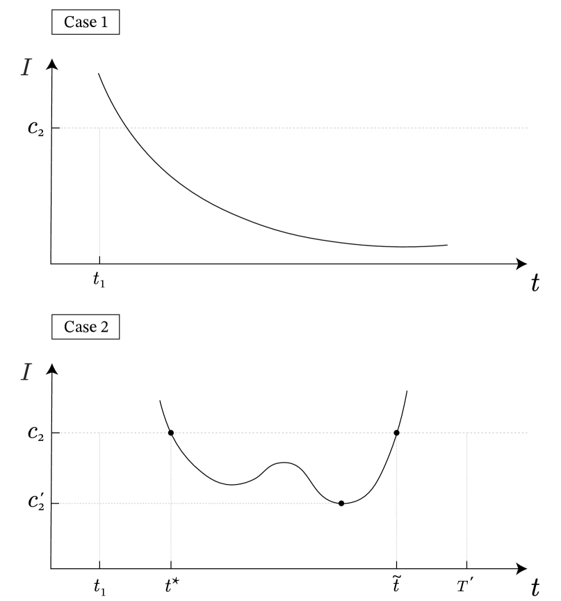
   Figure 6. Illustration of Cases 1 and (2a).

Case (1) Assuming that $I(t)<c_{2}$ for all $t\geq t_{1}$, by including the $-\beta_{0}c_{2}S(t)<0$ in (12) we get:

$$\begin{array}[]{lcl}\begin{cases}\vskip 12.0pt plus 4.0pt minus 4.0pt&\dot{S}\geq S(t)(A-S(t))-\beta_{0}c_{2}S(t)\quad\,,\qquad t\neq nT\\ &S(t^{+})\geq(1-p)S(t)\qquad\qquad\quad\,\,\,\,\,,\qquad t=nT.\end{cases}\end{array}$$

Now, let $z(t)$ be the solution of the following system:

$$\begin{array}[]{lcl}\begin{cases}\vskip 12.0pt plus 4.0pt minus 4.0pt&\dot{z}(t)=z(t)(A-z(t))-\beta_{0}c_{2}z(t)\qquad\,,\qquad t\neq nT\\ &z(t^{+})=(1-p)z(t)\qquad\qquad\qquad\quad\,\,\,\,,\qquad t=nT.\end{cases}\end{array}$$ (35)

Solving (35) as in (12), for $c_{2}>0$ arbitrarily small, we conclude that it has a periodic solution given explicitly by

$$\mathcal{Z}(t) = \dfrac{K}{1+\dfrac{p}{K\Big{(}(1-p)-e^{-KT}\Big{)}}Ke^{-K(t-nT)}}$$

$$= \dfrac{K}{1+\dfrac{p}{(1-p)-e^{-KT}}e^{-K(t-nT)}}$$

$$= \dfrac{K\Big{(}(1-p)-e^{-KT}\Big{)}}{(1-p)-e^{-KT}+pe^{-K(t-nT)}},$$

where $nT\leq t<(n+1)T$, $t>t_{1}$, $n\in{\mathbb{N}}$ and

$$K\coloneqq-\beta_{0}c_{2}+A.$$

Now it is easy to conclude that $S(t)\geq z(t)$, $S(0^{+})\geq z(0^{+})$, and $z(t)\longrightarrow\mathcal{Z}(t)$, in the pointwise convergence topology, where $\mathcal{Z}$ is the periodic solution of (35). Therefore there exist $\varepsilon_{1}>0$ (arbitrarily small) and $t_{2}>t_{1}$ such that $S(t)\geq z(t)>\mathcal{Z}(t)-\varepsilon_{1}$; from (8) and for $t>t_{2}$ we may write

$$\begin{array}[]{lcl}\begin{cases}\vskip 12.0pt plus 4.0pt minus 4.0pt&\dot{I}(t)\geq\Big{[}\beta_{0}\left(\mathcal{Z}(t)-\varepsilon_{1}\right)-(\sigma+g)\Big{]}I(t)\quad\,,\qquad t\neq nT\\ &I(nT^{+})=I(nT)\qquad\qquad\qquad\qquad\qquad,\qquad t=nT.\end{cases}\end{array}$$ (36)

Let $N\in{\mathbb{N}}$ and $NT\geq t_{2}$. Integrating (36) between $(nT,(n+1)T]$, $n\geq N$, we have

$$\int_{nT}^{(n+1)T}\dfrac{\mathrm{d}I(t)}{I(t)}\geq\int_{nT}^{(n+1)T}\Big{(}\beta_{0}\mathcal{Z}(t)-\beta_{0}\varepsilon_{1}-(\sigma+g)\Big{)}\,\mathrm{d}t$$

$$\Rightarrow \ln{\left(\dfrac{I\big{(}(n+1)T\big{)}}{I(nT)}\right)}\geq\int_{nT}^{(n+1)T}\beta_{0}\mathcal{Z}(t)\,\mathrm{d}t-\big{(}\beta_{0}\varepsilon_{1}+(\sigma+g)\big{)}T$$

$$\Leftrightarrow I\big{(}(n+1)T\big{)}\geq I(nT)\exp{\Big{\{}\int_{nT}^{(n+1)T}\beta_{0}\mathcal{Z}(t)\,\mathrm{d}t-\big{(}\beta_{0}\varepsilon_{1}+(\sigma+g)\big{)}T\Big{\}}}$$

$$\Leftrightarrow I\big{(}(n+1)T\big{)}\geq I(nT)\gamma,$$

where

$$\gamma=\exp{\left\{\int_{nT}^{(n+1)T}\beta_{0}\mathcal{Z}(t)\,\mathrm{d}t-\big{(}\beta_{0}\varepsilon_{1}+(\sigma+g)\big{)}T\right\}}.$$

Using induction over $N\in{\mathbb{N}}$ we get

$$I\big{(}(N+n)T\big{)}\geq I(NT)\,\gamma^{n}.$$ (37)

Claim: If $\mathcal{R}_{p}>1$, then $\gamma>1$.

Proof.

The proof follows from the chain of equivalences:

$$\mathcal{R}_{p}>1$$

$$\overset{\eqref{RpAND_Sc}\,\text{and}\,\varepsilon_{1}\gtrsim 0}{\Leftrightarrow} \dfrac{\beta_{0}}{\sigma+g}\dfrac{1}{T}\int_{nT}^{(n+1)T}(\mathcal{Z}(t)-\varepsilon_{1})\,\mathrm{d}t>1$$

$$\Leftrightarrow \beta_{0}\int_{nT}^{(n+1)T}(\mathcal{Z}(t)-\varepsilon_{1})\,\mathrm{d}t-(\sigma+g)T>0$$

$$\Leftrightarrow \exp{\Big{\{}\int_{nT}^{(n+1)T}\beta_{0}\mathcal{Z}(t)\,\mathrm{d}t-\big{(}\beta_{0}\varepsilon_{1}+(\sigma+g)\big{)}T\Big{\}}}>1$$

$$\Leftrightarrow \gamma>1.$$

∎

Since $\gamma>1$, we see that $0<I(NT)\,\gamma^{n}\longrightarrow\infty$ as $n\longrightarrow\infty$, which is a contradiction by Lemma 1. So, there exist $c_{2},T_{0}>0$ such that $I(t)>c_{2}$ for all $t\geq T_{0}$.

Case (2a) Let $t^{\star}=n_{1}T$, $n_{1}\in{\mathbb{N}}$. Then, $I(t)\geq c_{2}$ for $t\in[t_{1},t^{\star}]$ and $I({t^{\star}})=c_{2}$ and $I$ is decreasing. By Lemma 2, we have

$$\dot{I}(t)<0$$

$$\Leftrightarrow \beta_{0}(t)S(t)<\sigma+g$$

$$\overset{0<c_{1}\leq S(t)}{\Rightarrow} \beta_{0}(t)c_{1}<\sigma+g.$$

Hence, we can choose $n_{2},n_{3}\in{\mathbb{N}}$ such that $t^{\star}+n_{2}T>t_{1}$ and

$$\gamma^{n_{3}}\exp{\Big{\{}(\beta_{0}c_{1}-\sigma-g)n_{2}T\Big{\}}}>\gamma^{n_{3}}\exp{\Big{\{}(\beta_{0}c_{1}-\sigma-g)(n_{2}+1)T\Big{\}}}>1.$$

and define $T^{\prime}=n_{2}T+n_{3}T$.

Claim: There exists $t_{2}\in(t^{\star},t^{\star}+T^{\prime}]$ such that $I(t_{2})>c_{2}$.

Proof.

Let us assume that this is not true, i.e. that there is no such $t_{2}$.

Since $z(t)\longrightarrow\mathcal{Z}(t)$ as $t\longrightarrow\infty$ (in the pointwise convergence topology), as above, we may write $\mathcal{Z}(t)-\varepsilon_{1}<z(t)\leq S(t)$, for $t^{\star}+n_{2}T\leq t\leq t^{\star}+T^{\prime}$. From (36) and for $t^{\star}+n_{2}T\leq t\leq t^{\star}+T^{\prime}$, we have (see equation (37))

$$I(t^{\star}+T^{\prime})\geq I(t^{\star}+n_{2}T)\gamma^{n_{3}}.$$

From system (8), we get

$$\begin{array}[]{lcl}\begin{cases}\vskip 12.0pt plus 4.0pt minus 4.0pt&\dot{I}(t)\geq\left((\beta_{0}c_{1}-(\sigma+g)\right)I(t)\quad\quad\,\,\,\,,\qquad t\neq nT,\,\,\,\,n\in{\mathbb{N}}\\ &I(t^{+})=I(t)\qquad\qquad\qquad\qquad\quad\,\,\,,\qquad t=nT,\,\,\,\,n\in{\mathbb{N}}.\end{cases}\end{array}$$ (38)

for $t\in[t^{\star},t^{\star}+n_{2}T]$. Integrating (38) between $t^{\star}$ and $t^{\star}+n_{2}T$, we have:

$$\int_{t^{\star}}^{t^{\star}+n_{2}T}\dfrac{\mathrm{d}I(t)}{I(t)} \geq \int_{t^{\star}}^{t^{\star}+n_{2}T}\big{(}\beta_{0}c_{1}-(\sigma+g)\big{)}\,\mathrm{d}t$$

$$\Leftrightarrow I(t^{\star}+n_{2}T) \geq I(t^{\star})\exp{\big{\{}\big{(}\beta_{0}c_{1}-(\sigma+g)\big{)}n_{2}T\big{\}}}$$

$$\Leftrightarrow I(t^{\star}+n_{2}T) \geq c_{2}\exp{\big{\{}\left[\beta_{0}c_{1}-(\sigma+g)\right]n_{2}T\big{\}}},$$

leading to

$$I(t^{\star}+T^{\prime})\geq c_{2}\exp{\big{\{}\left[\beta_{0}c_{1}-(\sigma+g)\right]n_{2}T\big{\}}}\gamma^{n_{3}}>c_{2},$$

which is a contradiction, since we have assumed that no $t\in(t^{\star},t^{\star}+T^{\prime}]$ exists such that $I(t)>c_{2}$. ∎

Let $\tilde{t}=\inf_{t>t^{\star}}\{I(t)>c_{2}\}$. Then, for $t\in(t^{\star},\tilde{t})$, $I(t)\leq c_{2}$ and $I(\tilde{t})=c_{2}$, since $I(t)$ is continuous and $I(t^{+})=I(t)$ when $t=nT$. For $t\in(t^{\star},\tilde{t})$, suppose

$$t\in(t^{\star}+(k-1)T,t^{\star}+kT],\quad k\in{\mathbb{N}}\quad\text{and}\quad k\leq n_{2}+n_{3}.$$

Therefore, from (38) we have

$$I(t) \geq I(t^{\star})\exp{\big{\{}(k-1)\left(\beta_{0}c_{1}-(\sigma+g)\right)T\big{\}}}\exp{\big{\{}\left(\beta_{0}c_{1}-(\sigma+g)\right)\left(t-(t^{\star}+(k-1)T)\right)\big{\}}}$$

$$\geq c_{2}\exp{\big{\{}k\left(\beta_{0}c_{1}-(\sigma+g)\right)T\big{\}}}$$

$$\geq c_{2}\exp{\big{\{}(n_{2}+n_{3})\left(\beta_{0}c_{1}-(\sigma+g)\right)T\big{\}}}.$$

Let $c_{2}^{\prime}=c_{2}\exp{\{(n_{2}+n_{3})(\beta_{0}c_{1}-(\sigma+g))T\}}<c_{2}$. This lower bound does not depend either on $t^{\star}$ or $\tilde{t}$. Hence, we have $I(t)\geq c_{2}^{\prime}$ for $t\in(t^{\star},\tilde{t})$ and then for all $t>t_{1}$. For $t>\tilde{t}$, the same argument can be extended to $+\infty$ since $I(\tilde{t})\geq c_{2}$ and $c_{2}^{\prime}$ does not depend on the interval. This is a contradiction. Hence, there exist $c_{2},T_{0}>0$ such that $I(t)>c_{2}$ for all $t\geq T_{0}$. The proof of Case (2b) is entirely analogous and it is left to the reader.

The Poincaré-Bendixson theorem for Impulsive planar flows [46, Theorem 3.9] says that the $\omega$–limit of (8) is either an equilibrium, a periodic solution or a union of saddles that are heteroclinically connected. The only equilibrium of (8) is the origin. In order to allow endemic $T$-periodic solutions for $F_{I}$, then $\displaystyle\dfrac{1}{T}\int_{0}^{T}\mathcal{S}(t)\,\mathrm{d}t=S_{c}$. In this case, we know that there is an implicit (positive) map  $\mathcal{I}\equiv\mathcal{I}(t)$, where $t\in\mathbb{R}_{0}^{+}$. Since there are no more candidates for $\omega$–limit sets, we have in the topological closure of the first quadrant the following limit sets:

$$(0,0),\,\,{(0,\mathcal{I})}\,\,\text{and}\,\,(\mathcal{S},\mathcal{I}).$$

Since $(0,0)$ is repulsive (by Proposition 3), $(\mathcal{S},0)$ is a saddle (attracting in the first component and repelling in the second), the solutions should converge to the endemic periodic solution $(\mathcal{S},\mathcal{I})$ whose explicit solution is not known.

Figure 7. Illustration of the existence of a degenerate saddle-node bifurcation at $p=p_{1}(T)$, for $T>0$ fixed.

11. Proof of (6) of Theorem A

For $x\geq 0$, it is easy to check that $\displaystyle F_{S}^{\prime}(x)=\frac{P(x)}{Q^{2}(x)}$, where

$$P(x)=A(1-p)e^{AT}(x(e^{AT}-1)+A)-Ax(1-p)e^{AT}(e^{AT}-1)$$

and

$$Q(x)=x(e^{AT}-1)+A.$$

In particular, we have $F^{\prime}_{S}(0)=(1-p)e^{AT}$. Since

$$(1-p)e^{AT}=1\quad\Leftrightarrow\quad p=p_{1}(T),$$

then we conclude that $p_{1}$ corresponds to a saddle-node bifurcation of $F_{S}$ at $x=0$. Indeed, if $p>p_{1}$, then the map $F_{S}$ does not have fixed points besides $x=0$; if $p<p_{1}$, then one extra fixed point emerges, as shown in Figure 7. In terms of $p_{2}$, if $p>p_{2}$, then the periodic solution $(\mathcal{S},0)$ changes its stability because the Floquet multiplier $\lambda_{2}$ (cf. (30)) crosses the unit circle; this is why we have a transcritical bifurcation at $p=p_{2}$.

12. Proof of (7) of Theorem A

Item (7) is proved in Lemmas 7 and 8 of Section 6.

13. Proof of Corollary 1

For $\gamma,\omega>0$ and $A>S_{c}$, there is a hyperbolic $T$-periodic solution $(\mathcal{S},0)$ whose existence does not depend on $\beta_{\gamma}$. Therefore, it exists if $p>p_{1}(T)$ by Lemma 5. However, the region of the phase space where it is stable depends on $\gamma$. Indeed,

$$\lambda_{2}<1$$

$$\overset{\eqref{eigenvalue2},\text{ adapted}}{\Leftrightarrow} \exp{\left\{\displaystyle\int_{0}^{T}\beta_{\gamma}(t)\mathcal{S}(t)\,\mathrm{d}t-\left(\sigma+g\right)T\right\}}<1$$

$$\Leftrightarrow \displaystyle\int_{0}^{T}\beta_{0}\left(1+\gamma\Psi(\omega t)\right)\mathcal{S}(t)\,\mathrm{d}t-\left(\sigma+g\right)T<0$$

$$\Leftrightarrow \displaystyle\int_{0}^{T}\beta_{0}\mathcal{S}(t)\,\mathrm{d}t+\int_{0}^{T}\beta_{0}\gamma\Psi(\omega t)\mathcal{S}(t)\,\mathrm{d}t<\left(\sigma+g\right)T$$

$$\overset{\eqref{S_c(def)}}{\Leftrightarrow} \displaystyle\frac{1}{S_{c}T}\int_{0}^{T}\mathcal{S}(t)\,\mathrm{d}t+\frac{1}{S_{c}T}\int_{0}^{T}\gamma\Psi(\omega t)\mathcal{S}(t)\,\mathrm{d}t<1$$

$$\overset{\eqref{integral_S_til}}{\Leftrightarrow} \displaystyle\frac{1}{S_{c}T}\left[\ln{(1-p)}+AT\right]+\frac{1}{S_{c}T}\int_{0}^{T}\gamma\Psi(\omega t)\mathcal{S}(t)\,\mathrm{d}t<1$$

$$\Leftrightarrow \displaystyle\left[\ln{(1-p)}+AT\right]+\gamma\int_{0}^{T}\Psi(\omega t)\mathcal{S}(t)\,\mathrm{d}t<S_{c}T$$

$$\Leftrightarrow p>1-\exp{\left\{-\left[(A-S_{c})T+\gamma\int_{0}^{T}\Psi(\omega t)\mathcal{S}(t)\,\mathrm{d}t\right]\right\}}$$

$$\Leftrightarrow p>p_{2}^{\text{seas}}(T).$$

14. Proof of Theorem B

The proof follows from the item (4) of Theorem A combined with [41, Theorems 1 and 2], taking into account the following considerations:

• $\omega\in\mathbb{R}^{+}$ plays the role of “shear” of [41];

• the term $\beta_{\gamma}(t)=\beta_{0}\left(1+\gamma\Psi(\omega t)\right)>0$ may be seen as the radial “kick” of (8) that is periodic in time;

• the non-autonomous periodic forcing of (8) has nondegenerate critical points (by (C4)) – this avoids constant maps;

• the endemic periodic solution $(\mathcal{S},\mathcal{I})$ of (4) of Theorem A is globally attracting for (8).
  

For $\gamma>0$, equation (3) is equivalent to

$$\begin{array}[]{lcl}\dot{x}=f_{\gamma}(x)\quad\Leftrightarrow\quad\begin{cases}\vskip 6.0pt plus 2.0pt minus 2.0pt&\dot{S}=S(A-S)-\beta_{\gamma}IS\\ \vskip 6.0pt plus 2.0pt minus 2.0pt&\dot{I}=\beta_{\gamma}IS-\left(\sigma+g\right)I,\qquad\qquad\qquad t\neq nT\\ \vskip 12.0pt plus 4.0pt minus 4.0pt&\dot{\theta}=\omega\pmod{2\pi}\\ \vskip 6.0pt plus 2.0pt minus 2.0pt&S(nT)=(1-p)S(nT^{-})\\ \vskip 6.0pt plus 2.0pt minus 2.0pt&I(nT)=I(nT^{-}),\qquad\qquad\qquad\qquad t=nT,\end{cases}\end{array}$$ (39)

whose flow lies in $(\mathbb{R}_{0}^{+})^{2}\times\mathbf{S}^{1}$, where $\mathbf{S}^{1}\equiv\mathbb{R}\mod{\pi/\omega}$. Since the kicks are radial, they do not affect the $\theta$–coordinate. The following argument follows from [51, 52] and Section 3.2 of [47].

Using item (4) of Theorem A applied to the amplitude component of (39), one knows that the $\omega$-limit of Lebesgue almost all solutions of (39) is a strict subset of a two-dimensional attracting torus $\mathcal{T}_{0}$ (normally hyperbolic manifold). The torus is born ergodic when $T$ is not commensurable with $\omega/\tau$. Furthermore, for a dense set $\Delta$ of pairs $(T,\omega)\in[T_{2},+\infty)\times\mathbb{R}^{+}$ such that $T=k\tau/\omega$, one knows that this normally hyperbolic manifold is foliated by periodic solutions, as depicted on the left-hand side of Figure 8. In the terminology of Herman [48], the set $\Delta$ corresponds to orbits with rational rotation number.

Let $\Sigma$ be a cross-section to $\mathcal{T}_{0}$ where the first return is well defined. It is easy to observe that the set $\Sigma\cap\mathcal{T}_{0}$ is part of a circle. If $(T,\omega)\in\Delta$ and $\gamma=0$, there is at least one pair of periodic solutions in $\mathcal{T}_{0}$ which are heteroclinically connected, say $q_{1}$ (saddle) and $q_{2}$ (sink). The rotation number remains constant within a synchronization zone (valid for $\gamma>0$), also known as Arnold’s tongue [49].

Since $\mathcal{T}_{0}$ is a normally hyperbolic manifold, then for $\gamma\gtrsim 0$, there is a manifold $\mathcal{T}_{\gamma}$ diffeomorphic to $\mathcal{T}_{0}$, which is still attracting; as $\gamma$ increases further, the set $\Sigma\cap\mathcal{T}_{\gamma}$ becomes “non-smooth” and three generic scenarios may occur:

• the circle loses its smoothness (near $q_{2}$) when a pair of multipliers of the cycle becomes complex (non-real) or one of the multipliers is negative. At the moment of bifurcation, the length of an invariant circle becomes infinite and the torus is destroyed. The transition to chaos can come either from a period-doubling bifurcation cascade or via the breakdown of a torus occurring near $q_{2}$ (route A of [52, pp.124]);
  

• homo or heteroclinic tangle of the dissipative saddle $q_{1}$ (route B of [52, pp.124]);
  

• distortion of the unstable manifold near a non-hyperbolic saddle-node; the torus becomes non-smooth (route C of [52, pp.124]).
  

Following [52], the three mechanisms of torus destruction leads to a (non-hyperbolic) topological horseshoe-type map with a smooth bend. They do not cause the absorbing area to change abruptly and thus represent the bifurcation mechanism of a soft transition to chaos. The torus destruction line in the two control parameter plane $(\omega,\gamma)$ is characterised by a complex structure [51, 52]. There are small regions (in terms of measure) inside the resonance wedges where chaotic trajectories are observable: they correspond to strange attractors of Hénon type and are associated with historic behavior. Other stable points with large period exist as a consequence of the Newhouse phenomena. For a better understanding of Route (B), see Figure 8. Compare also with Figure 2.10 of [52].

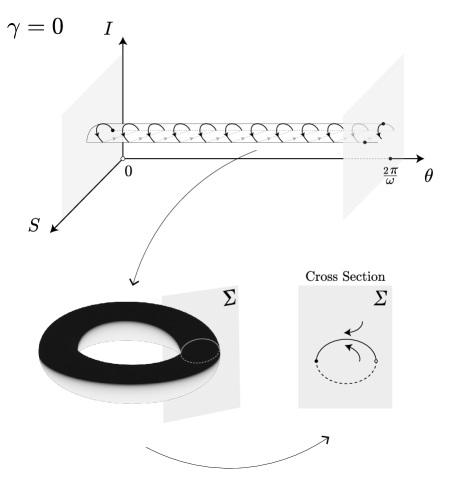
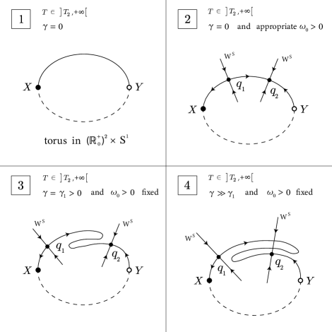
Figure 8. Sketch for the proof of Theorem B: (1). Torus bifurcation for $\gamma=0$. (2). For $\gamma=0$ and an appropriate $\omega\in\mathbb{R}^{+}$, we observe the emergence of periodic solutions represented by $q_{1}$ and $q_{2}$ on $\mathcal{T}_{0}$. (3 and 4). As $\gamma$ increases, the intersection $\Sigma\cap\mathcal{T}_{0}$ starts to lose its smoothness. In (4), the unstable manifold $W^{u}(q_{1})$ intersects the stable manifold $W^{s}(q_{2})$, leading to the formation of homoclinic tangles that indicate the emergence of horseshoes (chaos) – compare with Figure 2.10 of [51].

15. Numerics

In this section we perform some numerical simulations to illustrate the contents of Theorems A and B. All simulations were performed via MATLAB_R2018a software.

Figure 9: Numerical simulation of the five scenarios of system (8) illustrated in the bifurcation diagram $(T,p)$ in Figure 2 with initial condition $(S_{0},I_{0})=(0.5,0.4)$ described by Theorem A. The figure shows the behavior of the Susceptible and Infectious over time for different values of $p$ and corresponding phase space. Parameter values: $A=1$, $\beta_{0}=0.9$, $\sigma=0.2$, $g=0.5$, $T=4$ and $p\in[0,1]$. The green line represents the disease-free non-trivial periodic solution $(\mathcal{S},0)$, and the red line represents the endemic periodic solution $(\mathcal{S},\mathcal{I})$.

Figure 10: Projection of the solution of (39) with initial condition $(S_{0},I_{0},\theta_{0})=(0.5,0.4,0)$ for different values of $\gamma$. The parameter values are strategically chosen in order to have the dynamics of Region ③ of Figure 2: $A=1$, $\beta_{0}=0.2$, $\sigma=0.05$, $g=0.02$, $T=1$, $\omega=0.1$ and $p=0.5$. The dynamics of $S$ and $I$ show that the system tends towards the disease-free periodic solution $(\mathcal{S},0)$. As the amplitude of the seasonal variation $\gamma$ increases, the disease-free periodic solution starts to deform.

Figure 11: Numerical simulation of the phase space $(S,I)$, $(S,I,\theta)$, and respective cross-section ($\theta=2$) for three different values of $\gamma$ of (39). Parameter values used in this simulation: $A=1$, $T=4$, $\beta_{0}=2$, $\omega=6$, $\sigma=0.2$, $g=0.5$ and $p=0.4$ with initial condition $(S_{0},I_{0},\theta_{0})=(0.4074,0.2645,0)$. This simulation corresponds to Region ④, where $\mathcal{R}_{p}>1$. For this initial condition and $\gamma=4.89$, there is a positive Lyapunov exponent (0.13).

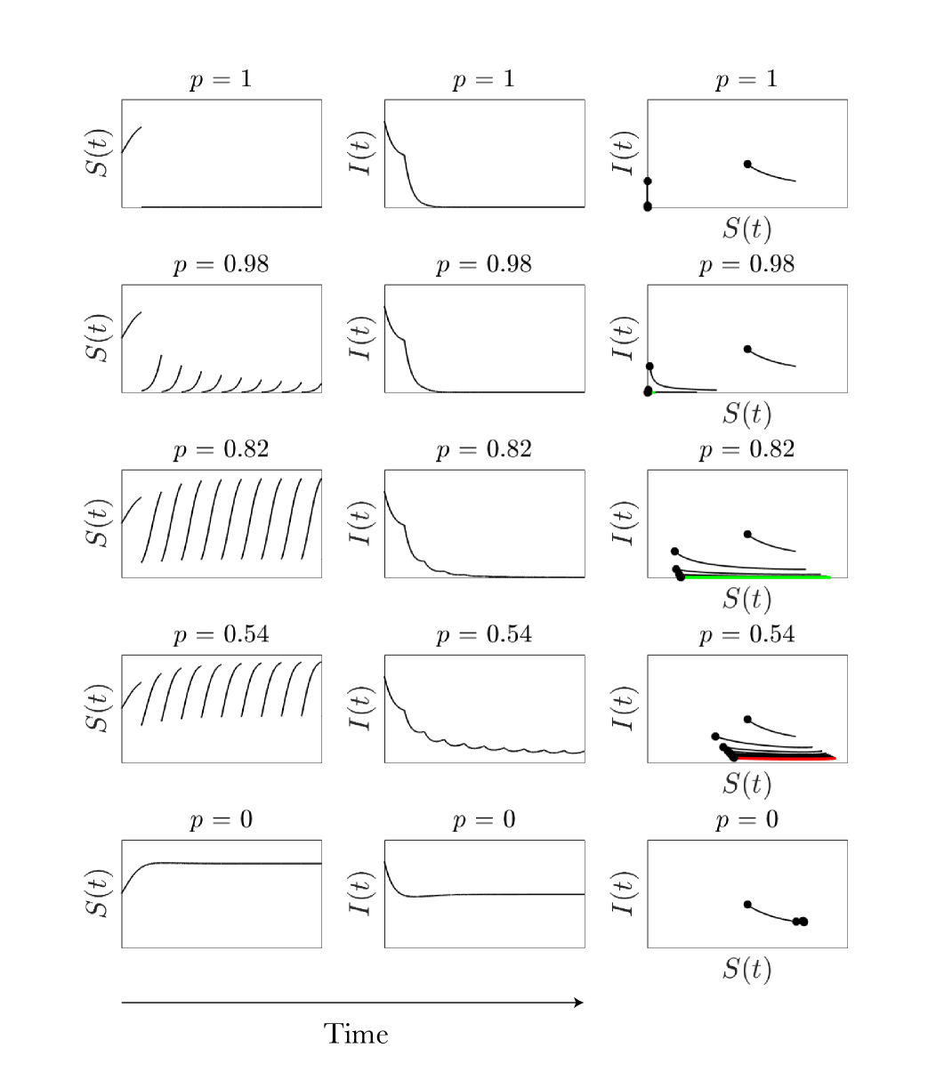
Figure 9. Numerical simulation of the five scenarios of system (8) illustrated in the bifurcation diagram $(T,p)$ of Figure 2 with initial condition $(S_{0},I_{0})=(0.5,0.4)$. The figure shows the behavior of the Susceptible and Infectious over time for different values of $p$ and corresponding phase space. Parameter values: $A=1$, $\beta_{0}=0.9$, $\sigma=0.2$, $g=0.5$, $T=4$ and $p\in[0,1]$. The green line represents the disease-free non-trivial periodic solution $(\mathcal{S},0)$, and the red line represents the endemic periodic solution $(\mathcal{S},\mathcal{I})$.

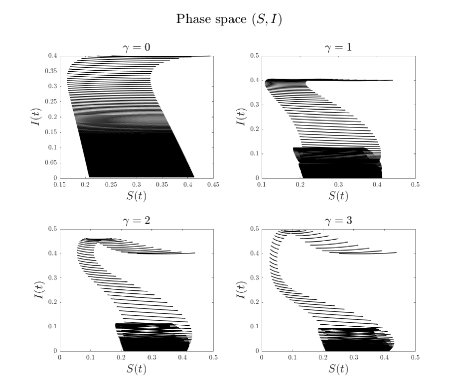
Figure 10. Projection of the solution of (39) with initial condition $(S_{0},I_{0},\theta_{0})=(0.5,0.4,0)$ for different values of $\gamma$. The parameter values are strategically chosen in order to have the dynamics of Region ③ of Figure 2: $A=1$, $\beta_{0}=0.2$, $\sigma=0.05$, $g=0.02$, $T=1$, $\omega=0.1$ and $p=0.5$. The dynamics of $S$ and $I$ show that the system tends towards the disease-free periodic solution $(\mathcal{S},0)$.

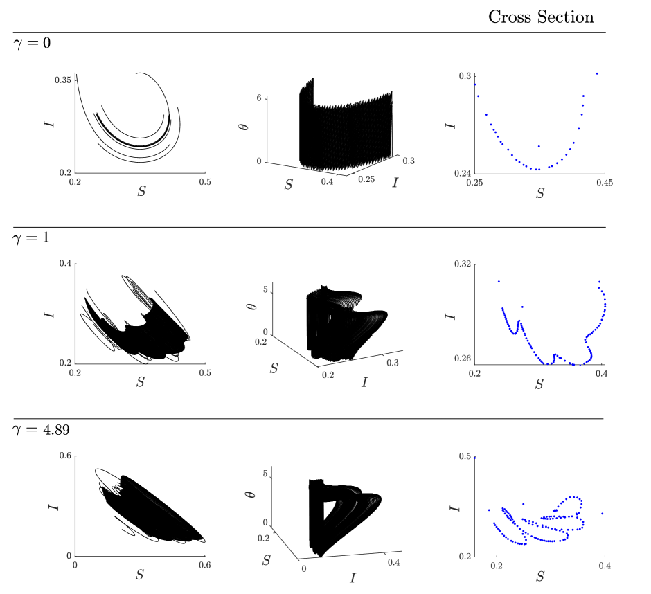
Figure 11. Numerical simulation of the phase space $(S,I)$, $(S,I,\theta)$, and respective cross-section ($\theta=2$) for three different values of $\gamma$ of (39). Parameter values used in this simulation: $A=1$, $T=4$, $\beta_{0}=2$, $\omega=6$, $\sigma=0.2$, $g=0.5$ and $p=0.4$ with initial condition $(S_{0},I_{0},\theta_{0})=(0.4074,0.2645,0)$. This simulation corresponds to Region ④, where $\mathcal{R}_{p}>1$. The system exhibits chaos if $\gamma=4.89$ with a positive Lyapunov exponent $0.13$.

16. Discussion and Final Remarks

In this work, we have studied a modified SIR model, introducing logistic growth to the population of the Susceptible individuals and incorporating pulse vaccination (Susceptible individuals are $T$-periodically vaccinated), conferring immunity to a proportion $p$ of the Susceptible population. Additionally, we have explored the model with and without seasonality into the disease transmission rate.

Results

Regarding our first main result (Theorem A), in the absence of seasonality in the disease transmission rate ($\gamma=0$), the analysis of the model reveals five stationary scenarios, depicted in the $(T,p)$ bifurcation diagram of Figures 2 and 9. All periodic $\omega$-limit sets have the same period as the initial pulse.

For $p=0$, the outcomes align with those of [10]: the $\omega$-limit of Lebesgue almost solutions is the endemic equilibrium. For $T>0$ fixed and values of $p$ between $\mathrm{𝟎}$ and $p_{2}(T)$, our model is permanent. In this case, the associated basic reproduction number is greater than 1. This agrees well with the findings of [16, 43, 44]. Our contribution goes further in this direction; using the Poincaré-Bendixson for impulsive flows, we have proved the existence of an endemic $T$-periodic solution.

For $p\in(p_{2}(T),p_{1}(T))$, system (3) exhibits a disease-free non-trivial periodic solution, where the curves $p=p_{1}(T)$ and $p=p_{2}(T)$ correspond to bifurcation thresholds (saddle-node and transcritical, respectively).

Under the effect of seasonality in the disease transmission rate, if $p<p_{2}(T)$,  $k\tau/\omega=T$ (within a resonance wedge), and $\gamma\gg 0$ (large), Theorem B indicates that the flow of (3) exhibits a suspended topological horseshoe. Consequently, the number of the Infectious persists and is more difficult to control the disease. The proof of this result follows the same lines of [52]. Our results stress that insufficient vaccination coverage combined with seasonality can generate chaotic dynamics.

We have presented numerical simulations to demonstrate that the periodic nature of pulse vaccination combined with seasonality might spread of the disease. Corollary 1 and Figure 4 warn that neglecting the effect of the amplitude of the seasonal transmission, the optimal pulse period could be an over-optimistic approximation [40].

Literature

In a recent study of a SIR model with pulse vaccination, the author of [45] pointed out two mechanisms that lead a classical SIR model to chaotic dynamics with low vaccine coverage. The first mechanism arises from the interaction of low birth and death rates combined with a high contact rate between individuals. The second mechanism results from high birth and low contact rates.

In our paper, we have analytically proved the emergence of chaos through a different technique: modulating the contact rate of the disease through a periodic function (seasonality), system (3) may exhibit chaos under generic assumptions. Mathematically, the author of [45] proved chaos via the Zanolin’s method [50] (stretching rectangles along paths); in our paper, chaos emerges via Torus-breakdown theory ([51] and [52, §2.1.4]).

Pulse vs. constant vaccination

We compare the findings of [10, 12] with the present work. Pulse vaccination requires a smaller percentage of people vaccinated to prevent a possible epidemic outbreak. Since pulse vaccination is periodic, it is enough to vaccinate a proportion $p$ of the population to keep the number of Susceptible individuals below prescribed epidemic limits. On the other hand, constant vaccination requires a high rate of Susceptible individuals to be vaccinated to avoid spreading the disease.

While constant vaccination offers constant and stable protection to the population, pulse vaccination can lead to poorly planned epidemic outbreaks, especially if the number of Susceptible individuals exceeds epidemic limits.

Open problem

Since $C^{2}$-hyperbolic horseshoes have zero Lebesgue measure, it is possible for a map to have a horseshoe, and at the same time, the orbit of Lebesgue-almost every point tends to a sink. Adapting the proof of [41] we conjecture that (concerning system (4)) if $\omega$ is large enough, then

$$\liminf_{\varepsilon\rightarrow 0^{+}}\,\,\frac{Leb\left\{\gamma\in[0,\varepsilon]:{f}_{\gamma}\text{ exhibits a strange attractor in the sense of \cite[cite]{[\@@bibref{}{WangYoung2003}{}{}]}}\right\}}{\varepsilon}>0,$$

where Leb denotes the one-dimensional Lebesgue measure. Inside the strange attractor, orbits jump around in a seemingly random fashion, and the future of individual orbits appears entirely unpredictable. For these chaotic attractors, however, there are laws of statistics that control the asymptotic distributions of Lebesgue almost all orbits in the basin of attraction of the attractor.

Final remarks and Future work

Our study suggests that the effective strategy for controlling an infectious disease governed by (3) must be in a way that the proportion $p$ of vaccination is at the target level needed for the disease eradication, and the time $T$ between doses must be appropriate. The results suggest that maintaining a high proportion $p$ of vaccination and optimizing the period $T$ for two doses of vaccine shall increase the effectiveness of the vaccination strategy. The inclusion of seasonality has dramatic impacts on the dynamics.

One of the main challenges of the World Health Organization is the global eradication of certain diseases in countries with low incomes and high birth rates. From an applied perspective, our results could be helpful for the optimal design of vaccination programs.

Further refinements of the pulse vaccination strategy need to take seasonal disease dynamics into full account. From a theoretical perspective, there is a need to develop analytical epidemiological models that incorporate information such as the natural period of the disease under analysis (resonance dynamics of [40]).

References

- [1] Hethcote HW (2000) The Mathematics of Infectious Diseases. SIAM Rev. 42: 599–653
- [2] Cobey S (2020) Modeling infectious disease dynamics. Science 368:713–714
- [3] Kermack WO, McKendrick AG (1932) Contributions to the mathematical theory of epidemics. II. The problem of endemicity. Proc. R. Soc. Lond. 138: 55–83
- [4] Brauer F, Castillo-Chavez C (2012). Mathematical Models in Population Biology and Epidemiology. New York. Springer
- [5] Diekmann O, Heesterbeek JA, Britton T (2012) Mathematical Tools for Understanding Infectious Disease Dynamics. Princeton University Press.
- [6] van den Driessche P, Watmough J (2002) Reproduction numbers and sub-threshold endemic equilibria for compartmental models of disease transmission. Math. Biosci. 180: 29–48
- [7] Maurício de Carvalho JPS, Moreira-Pinto B (2021) A fractional-order model for CoViD-19 dynamics with reinfection and the importance of quarantine. Chaos Solitons Fractals 151: 111275
- [8] Plotkin SA (2005) Vaccines: past, present and future. Nat. Med. 11: S5–S11
- [9] Plotkin SA, Plotkin SL (2011) The development of vaccines: how the past led to the future. Nat. Rev. Microbiol. 9: 889–893
- [10] Maurício de Carvalho JPS, Rodrigues AA (2023) SIR Model with Vaccination: Bifurcation Analysis. Qual. Theory Dyn. Syst. 22: 32 pages
- [11] Makinde OD (2007) A domian decomposition approach to a SIR epidemic model with constant vaccination strategy. Appl. Math. Comput. 184: 842–848
- [12] Shulgin B, Stone L, Agur Z (1998) Pulse vaccination strategy in the SIR epidemic model. Bull. Math. Biol. 60: 1123–1148
- [13] Agur Z, Cojocaru L, Mazor G, Anderson RM, Danon YL (1993) Pulse mass measles vaccination across age cohorts. Proc. Natl. Acad. Sci. USA. 90: 11698–11702
- [14] Stone L, Shulgin B, Agur Z (2000) Theoretical examination of the pulse vaccination policy in the SIR epidemic model. Math. Comput. Model. 31: 207–215
- [15] Lu Z, Chi X, Chen L (2002) The Effect of Constant and Pulse Vaccination on SIR Epidemic Model with Horizontal and Vertical Transmission. Math. Comput. Model. 36: 1039-1057
- [16] Meng X, Chen L (2008) The dynamics of a new SIR epidemic model concerning pulse vaccination strategy. App. Math. Comput. 197: 582–597
- [17] Jin Z, Haque M (2007) The SIS Epidemic Model with Impulsive Effects. Eighth ACIS International Conference on Software Engineering, Artificial Intelligence, Networking, and Parallel/Distributed Computing (SNPD 2007), Qingdao, China, 2007, pp. 505–507
- [18] Buonomo B, Chitnis N, d’Onofrio A (2018) Seasonality in epidemic models: a literature review. Ric. Di Mat. 67: 7–25
- [19] Maurício de Carvalho JPS, Rodrigues AAP (2022) Strange attractors in a dynamical system inspired by a seasonally forced SIR model. Phys. D 434: 12 pages
- [20] Keeling MJ, Rohani P, Grenfell BT (2001) Seasonally forced disease dynamics explored as switching between attractors, Physica D. 148: 317–335
- [21] Barrientos PG, Rodríguez JA, Ruiz-Herrera A (2017) Chaotic dynamics in the seasonally forced SIR epidemic model. J. Math. Biol. 75: 1655–1668
- [22] Duarte J, Januário C, Martins N, Rogovchenko S, Rogovchenko Y (2019) Chaos analysis and explicit series solutions to the seasonally forced SIR epidemic model. J. Math. Biol. 78: 2235–2258
- [23] Wang L (2015) Existence of periodic solutions of seasonally forced SIR models with impulse vaccination. Taiwan. J. Math. 19: 1713–1729
- [24] Feltrin G (2018). Mawhin’s Coincidence Degree. In: Positive Solutions to Indefinite Problems. Frontiers in Mathematics. Birkhäuser, Cham.
- [25] Wang L (2020) Existence of Periodic Solutions of Seasonally Forced SEIR Models with Pulse Vaccination. Discrete Dyn. Nat. Soc. 2020: 11 pages
- [26] Jódar L, Villanueva RJ, Arenas A (2008) Modeling the spread of seasonal epidemiological diseases: Theory and applications
- [27] Zu J, Wang L (2015) Periodic solutions for a seasonally forced SIR model with impact of media coverage. Adv. Differ. Equ. 2015: 10 pages
- [28] Dishliev A, Dishlieva K, Nenov S (2012) Specific asymptotic properties of the solutions of impulsive differential equations. Methods and applications. Academic Publication, 2012
- [29] Lakshmikantham V, Bainov DD, Simeonov PS (1989) Theory of Impulsive Differential Equations. Series in Modern Applied Mathematics: Vol. 6. World Scientific
- [30] Agarwal R, Snezhana H, O’Regan D (2017) Non-instantaneous impulses in differential equations Springer, Cham. 1–72, 2017
- [31] Bainov D, Simeonov P (1993) Impulsive differential equations: periodic solutions and applications. Vol. 66. CRC Press, 1993
- [32] Milev N, Bainov D (1990) Stability of linear impulsive differential equations. Comput. Math. Appl. 21: 2217–2224
- [33] Simeonov P, Bainov D (1988) Orbital stability of periodic solutions of autonomous systems with impulse effect. Int. J. Systems Sci. 19: 2561–2585
- [34] Hirsch MW, Smale S (1974) Differential Equations, Dynamical Systems and Linear Algebra. Academic Press: New York.
- [35] Dietz K (1976) The incidence of infectious diseases under the influence of seasonal fluctuations. In: Mathematical models in medicine. Springer Berlin Heidelberg, pp 1–15
- [36] Li J, Teng Z, Wang G, Zhang L, Hu C (2017) Stability and bifurcation analysis of an SIR epidemic model with logistic growth and saturated treatment. Chaos Solitons Fractals 99: 63–71
- [37] Zhang XA, Chen L (1999) The periodic solution of a class of epidemic models. Comput. Math. Appl. 38: 61–71
- [38] Li J, Blakeley D, Smith RJ. The failure of (2011) Comput. Math. Methods Med. 2011: 17 pages
- [39] Tang S, Chen L (2001) A discrete predator-prey system with age-structure for predator and natural barriers for prey. Math. Model. Numer. Anal. 35: 675–690
- [40] Choisy M, Guégan J-F, Rohani P (2006) Dynamics of infectious diseases and pulse vaccination: Teasing apart the embedded resonance effects. Phys. D 223: 26–35
- [41] Wang Q, Young LS (2003) Strange Attractors in Periodically-Kicked Limit Cycles and Hopf Bifurcations. Commun. Math. Phys. 240: 509–529
- [42] Iooss G, Joseph D (1980) Elementary Stability and Bifurcation Theory. New York. Springer
- [43] Yongzhen P, Shuping L, Changguo L, Chen S (2011) The effect of constant and pulse vaccination on an SIR epidemic model with infectious period. Appl. Math. Model. 35: 3866–3878
- [44] Zou Q, Gao S, Zhong Q (2009) Pulse Vaccination Strategy in an Epidemic Model with Time Delays and Nonlinear Incidence. Adv. Stud. Biol. 1: 307–321
- [45] Herrera AR (2023) Paradoxical phenomena and chaotic dynamics in epidemic models subject to vaccination. Commun. Pure Appl. Anal. 19: 2533–2548
- [46] Bonotto EM, Federson M (2008) Limit sets and the Poincaré-Bendixson Theorem in impulsive semidynamical systems. J. Differ. Equ. 244: 2334–2349
- [47] Wang Q, Young LS (2002) From Invariant Curves to Strange Attractors. Commun. Math. Phys. 225:275–304
- [48] Herman MR (1997) Mesure de Lebesgue et Nombre de Rotation. Lecture Notes in Mathematics. 597: 271–293, Springer, Berlin
- [49] Shilnikov A, Shilnikov L, Turaev D (2004) On some mathematical topics in classical synchronization: A tutorial. Int. J. Bifurc. Chaos Appl. 14: 2143–2160
- [50] Margheri A, Rebelo C, Zanolin F (2010) Chaos in periodically perturbed planar Hamiltonian systems using linked twist maps. J. Differ. Equ. 249: 3233–3257
- [51] Anishchenko VS, Safonova MA, Chua LO (1993) Confirmation of the Afraimovich-Shilnikov torus-breakdown theorem via a torus circuit. IEEE Trans. Circuits Syst. I Fundam. Theory Appl. 40: 792–800
- [52] Anishchenko VS, Astakhov V, Neiman A, Vadivasova T, Schimansky-Geier L (2007) Nonlinear dynamics of chaotic and stochastic systems. Springer Series in Synergetics (second). Springer, Berlin