Higher Memory Effects in Numerical Simulations of Binary Black Hole Mergers

Abstract

Gravitational memory effects are predictions of general relativity that are characterized by an observable effect that persists after the passage of gravitational waves. In recent years, they have garnered particular interest, both due to their connection to asymptotic symmetries and soft theorems and because their observation would serve as a unique test of the nonlinear nature of general relativity. Apart from the more commonly known displacement and spin memories, however, there are other memory effects predicted by Einstein’s equations that are associated with more subleading terms in the asymptotic expansion of the Bondi-Sachs metric. In this paper, we write explicit expressions for these higher memory effects in terms of their charge and flux contributions. Further, by using a numerical relativity simulation of a binary black hole merger, we compute the magnitude and morphology of these terms and compare them to those of the displacement and spin memory. We find that, although these terms are interesting from a theoretical perspective, due to their small magnitude they will be particularly challenging to observe with current and future detectors.

I Introduction

The “displacement” gravitational wave memory effect arises as a permanent change in the separation of two observers due to the passage of gravitational waves. This effect was first postulated in the linearized regime Zel’dovich and Polnarev (1974), but for bound systems, the predominant effect is sourced by nonlinear effects in the propagation of gravitational waves Christodoulou (1991); Thorne (1992). This effect is difficult to detect both because of its low-frequency nature and that it is simply smaller in amplitude than the predominantly oscillatory part of the gravitational wave signal. However, there have been numerous proposals to measure it using both ground-based detectors (by stacking multiple signals in current detectors Lasky et al. (2016); Boersma et al. (2020); Grant and Nichols (2023), which has been performed explicitly in Refs. Hübner et al. (2020, 2021)) or from single events in future detectors Johnson et al. (2019); Grant and Nichols (2023). It should also be seen by space-based detectors Islo et al. (2019); Ghosh et al. (2023) and pulsar timing arrays, and the latter currently provide upper bounds on the memory coming from the stochastic background Agazie et al. (2023).

In addition to the displacement memory, a variety of other effects appearing as permanent changes in some idealized detector have been considered. These effects all fall under the class of so-called “persistent observables” Flanagan et al. (2019), the simplest subset of which forms the so-called “curve deviation”. In Ref. Grant and Nichols (2022), it was found that the curve deviation could be written in terms of a set of quantities at null infinity that are temporal moments of the Bondi news: a tensor which characterizes the presence of radiation at null infinity. For the zeroth moment (that is, a single integral) of the news, this relationship was already known, and reflects the fact that integrating the news between early and late times gives the value of the displacement memory effect. However, the curve deviation observable depends on higher moments of the news as well. For example, the “drift” memory (previously called “subleading displacement memory” Flanagan et al. (2019): see Ref. Grant for an explanation for the change in terminology), which described the separation of two observers with a nonzero initial relative velocity, was related to the first and zeroth moments of the news. Similarly, higher moments of the news could be used to determine the dependence of the final separation on the initial relative acceleration and higher derivatives. Collectively, we refer to these higher moments of the news as “higher memory effects”.

Furthermore, an important result of Ref. Grant and Nichols (2022) was that these moments of the news could be written in terms of a “charge” contribution and a “flux” contribution, which generalizes the usual linear/nonlinear or ordinary/null Bieri and Garfinkle (2014) splittings of the displacement memory. For the first moment, such a decomposition was already known as well, as it was shown for spin Pasterski et al. (2016); Nichols (2017) and center-of-mass Nichols (2018) memories, which form the magnetic and electric parts of the drift memory. That such a splitting could be achieved for all higher memory effects, however, was a novel result, and follows from the asymptotic form of the Einstein equations.

There is another, useful formulation of the displacement memory in terms of asymptotic symmetries. Here, for each spherical harmonic mode, the charge contribution can be thought of as the change in a charge constructed from a member of the supertranslation subalgebra of the Bondi-Metzner-Sachs (BMS) algebra—the symmetry algebra at null infinity. Understanding the drift memory in this way, however, requires an extension of the BMS algebra into either of the “extended” Barnich and Troessaert (2010) or “generalized” Campiglia and Laddha (2014) BMS algebras, and many issues with these extensions have been pointed out in the literature Flanagan and Nichols (2017); Flanagan et al. (2020); Elhashash and Nichols (2021). Recently, an infinite set of charges were also defined which form a representation of the algebra $Lw_{1+\infty}$ Freidel et al. (2022a), and at linear order these charges can be shown Compère et al. (2022) to be equivalent to those in Ref. Grant and Nichols (2022). While these connections to symmetry algebras are interesting, we do not discuss them further in this paper, as everything that we present can be straightforwardly derived from the Einstein equations.

An important question remains about the status of this split into charge and flux contributions: for a given system, which is larger? This is important for observing the memory effect, by the following argument Grant and Nichols (2023). For simplicity, we restrict to a discussion of the displacement memory, although similar arguments for higher moments also apply. First, note that by “detecting the displacement memory”, one does not mean “measuring some finite offset in the detector”, as current ground-based detectors are only sensitive in some frequency range that does not include zero. Instead, one should try to detect a part of the signal which contributes to this finite offset, which one could call the time-dependent “memory signal”. In the case of the displacement memory, it happens to be the case that, for binary mergers, it is the flux contribution which makes the largest contribution (for the $m=0$ modes) to the zeroth moment of the news (see, for example, Ref. Mitman et al. (2020)). Moreover, since this contribution as a function of time is non-oscillatory and looks like a smoothed out step function, it is a reasonable choice for the time-dependent “displacement memory signal”.

When considering higher moments of the news, one is faced with another issue: current ground-based gravitational wave detectors are sensitive to the shear, and not any particular integrals of the news. If one is given the $n$th moment of the news as a function of time, one can obtain the shear as a function of time (up to an arbitrary constant) by differentiating $n$ times. As such, the question of which is the larger contribution should be asked of the $n$th derivative of the charge or flux. For the case of the spin memory (the magnetic part of the first moment of the news), it is once again the flux contribution that is larger. Furthermore, this contribution is again non-oscillatory Mitman et al. (2020) (in the $m=0$ modes) and resembles a single bump, i.e., a smoothed-out delta function.

Motivated by these considerations, we seek to answer the following questions for the higher memory effects:

1. Which contribution to the shear, charge or flux, is more important?

2. Is it always the case that the charge contributions are primarily oscillatory, and the flux contributions are primarily non-oscillatory?

3. What is the general morphology of these non-oscillatory contributions?

As there are an infinite number of these higher memory effects, we restrict our attention to the displacement memory (zeroth moment), drift memory (first moment), and the second moment of the news. To explore these inquiries, we will examine the waveforms produced by numerical relativity simulations of binary black hole mergers that have been run using the Simulating eXtreme Spacetimes (SXS) Collaboration’s SpEC code (to perform the Cauchy evolution) and SpECTRE code [to extract the asymptotic data via a Cauchy-characteristic evolution (CCE)] Deppe et al. (2023); Moxon et al. (2020, 2023).

The structure of this paper is the following. In Sec. II, we review the necessary material for this paper: Bondi-Sachs coordinates, the tetrad variables that we will work with (the shear $\sigma$ and modified Weyl scalars $\psi_{i}$), and the moments of the news. In Sec. III, we then show how one can (non-uniquely) define charges whose evolution gives these moments of the news, adapting the procedure in Ref. Grant and Nichols (2022) to be in terms of tetrad variables, instead of tensorial quantities. We also discuss the procedure for inverting the moments of the news in order to recover the shear. Finally, in Sec. IV, we discuss our numerical results for binary black hole mergers, showing the hierarchy of the various contributions to the shear, as well as their morphology. We present our conclusions in Sec. V.

In this paper, we set $G=c=1$ and adopt the mostly plus metric signature. We use Latin characters from the beginning of the alphabet ($a$, $b$, etc.) for abstract indices and Latin characters from the middle of the alphabet ($i$, $j$, etc.) in order to denote angular indices on the two-sphere.

II Background

II.1 Bondi-Sachs coordinates

In this paper, we work with asymptotic quantities defined with respect to a tetrad, and using the Geroch-Held-Penrose (GHP) formalism Geroch et al. (1973). For concreteness, though, we begin with the form of the metric in Bondi-Sachs coordinates, which we denote with $u$, $r$, and two arbitrary angular coordinates $\theta^{i}$. In vacuum general relativity, this metric takes the form (see, for example, Grant and Nichols (2022))

$$\mathrm{d}s^{2}=-\left(1-\frac{2V}{r}\right)e^{2\beta/r^{2}}\mathrm{d}u^{2}-2e^{2\beta/r^{2}}\mathrm{d}u\mathrm{d}r+r^{2}\left(\gamma h_{ij}+\frac{1}{r}\mathcal{C}_{ij}\right)\left(\mathrm{d}\theta^{i}-\frac{\mathcal{U}^{i}}{r^{2}}\mathrm{d}u\right)\left(\mathrm{d}\theta^{j}-\frac{\mathcal{U}^{j}}{r^{2}}\mathrm{d}u\right),$$ (1)

where $h_{ij}$ is the metric on the two-sphere (which we use to raise and lower $\theta^{i}$ indices). The scalar $\gamma$ is given by

$$\gamma=\sqrt{1+\frac{\mathcal{C}_{ij}\mathcal{C}^{ij}}{2r^{2}}},$$ (2)

which enforces the Bondi condition that the determinant of the angular part of the metric is constant in $r$. There are six remaining metric functions that arise through $V$, $\beta$, $\mathcal{U}^{i}$, and $\mathcal{C}_{ij}$ (which is trace-free with respect to $h_{ij}$). For this paper, $\beta$ is unimportant, but the remaining five have the following expansions:

$$V =m+\mathcal{M}/r,$$ (3a)

$$\mathcal{C}_{ij} =C_{ij}+\frac{1}{r^{2}}\mathcal{E}_{ij},$$ (3b)

$$\mathcal{U}^{i} =-\frac{1}{2}\mathscr{D}_{j}C^{ij}-\frac{1}{r}\bigg{[}\frac{2}{3}N^{i}-\frac{1}{16}\mathscr{D}^{i}(C_{jk}C^{jk})$$

$$\hskip 80.00012pt-\frac{1}{2}C^{ij}\mathscr{D}^{k}C_{jk}\bigg{]}+\frac{1}{r^{2}}\Upsilon^{i},$$ (3c)

where $\mathscr{D}_{i}$ is the derivative on the sphere compatible with $h_{ij}$. Note that, in terms of their $r$ dependence, $\mathcal{M}$, $\mathcal{E}_{ij}$, and $\Upsilon^{i}$ are all $O(1)$ functions of $r$, but $m$, $C_{ij}$, and $N^{i}$ are all constants. Again, $\mathcal{M}$ and $\Upsilon^{i}$ are unimportant for the discussion in this paper, but we write $\mathcal{E}_{ij}$ explicitly as a power series in $r$:

$$\mathcal{E}_{ij}=\sum_{n=0}^{\infty}\frac{1}{r^{n}}\underset{{}^{(n)}}{\mathcal{E}}{}_{ij}.$$ (4)

As a consequence of Einstein’s equations, the free data at null infinity in vacuum general relativity are the initial values of $m$, $N^{i}$, and each $\underset{{}^{(n)}}{\mathcal{E}}{}_{ij}$, together with the value of $C_{ij}$ at all times. Due to their importance, these quantities all have names:

• $m$ is the mass aspect, a generalization of the mass that is angle-dependent;

• $N^{i}$ is the angular momentum aspect, with a similarly intuitive explanation for its name;

• $C_{ij}$ is the shear, since (as we discuss later, in Sec. II.2) it is related to the shear in the GHP formalism; and

• $\underset{{}^{(n)}}{\mathcal{E}}{}_{ij}$ are the “higher Bondi aspects” Compère et al. (2022).

Moreover, the shear $C_{ij}$, being the $1/r$, traceless and transverse part of the metric, is related to the usual transverse-traceless metric that an observer will measure at large distances from a source. Finally, a quantity of great interest in these spacetimes is the news $N_{ij}$:

$$N_{ij}\equiv\partial_{u}C_{ij}.$$ (5)

This is the quantity which characterizes the presence of radiation in these spacetimes (see, for example, Refs. Geroch (1977); Wald and Zoupas (2000); Grant et al. (2022)).

II.2 GHP formalism

The GHP formalism involves writing the metric in terms of a null tetrad $\{l^{a},n^{a},m^{a},\bar{m}^{a}\}$, satisfying

$$l^{a}n_{a}=-1,\qquad m^{a}\bar{m}_{a}=1,$$ (6)

with all other contractions vanishing. The metric can then be written as

$$g_{ab}=-2l_{(a}n_{b)}+2m_{(a}\bar{m}_{b)}.$$ (7)

The main quantities of interest are the Weyl scalars $\Psi_{i}$, for $0\leq i\leq 4$, defined by

$$\Psi_{0} \equiv C_{abcd}l^{a}m^{b}l^{c}m^{d},$$ (8a)

$$\Psi_{1} \equiv C_{abcd}l^{a}n^{b}l^{c}m^{d},$$ (8b)

$$\Psi_{2} \equiv C_{abcd}l^{a}m^{b}\bar{m}^{c}n^{d},$$ (8c)

$$\Psi_{3} \equiv C_{abcd}l^{a}n^{b}\bar{m}^{c}n^{d},$$ (8d)

$$\Psi_{4} \equiv C_{abcd}n^{a}\bar{m}^{b}n^{c}\bar{m}^{d}.$$ (8e)

The conventions for these quantities are taken from Ref. Iozzo et al. (2021).

In terms of Bondi coordinates, the tetrad that is used by the SpECTRE code’s implementation of CCE is given by Eqs. (81) of Refs. Deppe et al. (2023); Moxon et al. (2020):

$$l^{a} \equiv\frac{1}{\sqrt{2}}(\partial_{r})^{a},$$ (10a)

$$n^{a} \equiv\sqrt{2}e^{-2\beta/r}\bigg{[}(\partial_{u})^{a}+\frac{1}{r^{2}}\mathcal{U}^{i}(\partial_{i})^{a}$$

$$\hskip 65.00009pt-\frac{1}{2}\left(1-\frac{2V}{r}\right)(\partial_{r})^{a}\bigg{]},$$ (10b)

$$m^{a} \equiv-\frac{1}{\sqrt{2}r}(\partial_{i})^{a}q_{j}\left(\sqrt{1+\gamma}h^{ij}-\frac{1}{r\sqrt{1+\gamma}}\mathcal{C}^{ij}\right).$$ (10c)

This tetrad is defined in terms of a complex dyad $q^{i}$ on the sphere, defined (in spherical coordinates) by

$$q^{i}\equiv-\frac{1}{\sqrt{2}}\left[(\partial_{\theta})^{i}+\frac{i}{\sin\theta}(\partial_{\phi})^{i}\right].$$ (11)

Note that this differs by a factor of $\sqrt{2}$ from the conventions in Ref. Moxon et al. (2020).

This dyad is also used to construct the spin-raising and -lowering operators $\eth$ and $\bar{\eth}$, as follows: suppose that one has a tensor $v_{i_{1}\cdots i_{p+q}}$ on the sphere. One can then define a complex scalar $v$ by

$$v\equiv v_{i_{1}\cdot i_{p}j_{1}\cdots j_{q}}q^{i_{1}}\cdots q^{i_{p}}\bar{q}^{j_{1}}\cdots q^{j_{q}};$$ (12)

under a dyad rotation $q^{i}\to e^{i\psi}q^{i}$, $v\to e^{is\psi}v$, where $s=p-q$ is the spin weight of $v$. The operator $\eth$ is then defined by

$$\eth v\equiv q^{i}q^{j_{1}}\cdots q^{j_{p}}\bar{q}^{k_{1}}\cdots\bar{q}^{k_{q}}\mathscr{D}_{i}v_{j_{1}\cdots j_{p}k_{1}\cdots k_{q}},$$ (13)

while $\bar{\eth}$ is defined by $\bar{\eth}v=\overline{\eth\bar{v}}$.

Note that, if $v$ has spin weight $s$, then $\eth v$ has spin weight $s+1$ and $\bar{\eth}v$ has spin weight $s-1$. As such, we can consider the eigenfunctions of $\eth\bar{\eth}$ (or, equivalently, $\bar{\eth}\eth$), which are the spin-weighted spherical harmonics ${}_{s}Y_{\ell m}$. In this paper, we will only need the following properties (using the conventions of the scri package Boyle et al. (2023)):

$$\eth{}_{s}Y_{\ell m} =\sqrt{\frac{(\ell-s)(\ell+s+1)}{2}}{}_{s+1}Y_{\ell m},$$ (14a)

$$\bar{\eth}{}_{s}Y_{\ell m} =-\sqrt{\frac{(\ell+s)(\ell-s+1)}{2}}{}_{s-1}Y_{\ell m},$$ (14b)

from which it follows that

$$\eth\bar{\eth}{}_{s}Y_{\ell m} =-\frac{(\ell+s)(\ell-s+1)}{2}{}_{s}Y_{\ell m},$$ (15a)

$$\bar{\eth}\eth{}_{s}Y_{\ell m} =-\frac{(\ell-s)(\ell+s+1)}{2}{}_{s}Y_{\ell m}.$$ (15b)

As such, we can invert the action of $\eth$ or $\bar{\eth}$ on an individual spin-weighted spherical harmonic through a combination of applying $\bar{\eth}$ or $\eth$ (respectively) and dividing by an appropriate $\ell$- and $s$-dependent coefficient:

$$\eth^{-1}{}_{s}Y_{\ell m} =-\frac{2}{(\ell+s)(\ell-s+1)}\bar{\eth}{}_{s}Y_{\ell m},$$ (16a)

$$\bar{\eth}^{-1}{}_{s}Y_{\ell m} =-\frac{2}{(\ell-s)(\ell+s+1)}\eth{}_{s}Y_{\ell m}.$$ (16b)

Note that these equations only provide an expression for $\eth^{-1}$ and $\bar{\eth}^{-1}$ acting on individual spin-weighted spherical harmonics. As such, whenever we are inverting $\eth$ or $\bar{\eth}$, we will first expand on a basis of these functions.

Finally, this dyad can be used to define the strain $h$ Mitman et al. (2020):

$$h\equiv r\bar{q}^{i}\bar{q}^{j}\mathcal{C}_{ij}.$$ (17)

This quantity is important, since the leading order piece of $h$, together with the leading order pieces of the Weyl scalars $\Psi_{i}$, form the output of the CCE code. In contrast, the quantities that are output by the scri package Boyle et al. (2023); Boyle (2013); Boyle et al. (2014); Boyle (2016), which we use throughout the remainder of this paper, are $\psi_{i}$ and $\sigma$, which are defined in terms of these quantities by

$$\psi_{i}\equiv\lim_{r\to\infty}r^{5-i}(-\sqrt{2})^{2-i}\Psi_{i},$$ (18)

$$\sigma\equiv\lim_{r\to\infty}\frac{\bar{h}}{2r}.$$ (19)

Note that these could be defined as (coefficients in an expansion in $1/r$ of) the Weyl scalars (for $\psi_{i}$) and shear (for $\sigma$), defined as in Ref. Geroch et al. (1973) with respect to some tetrad, but this is not important for the discussion of this paper.

There are simple relationships between the $\psi_{i}$ and $\sigma$ and the functions appearing in the metric in Eq. (1). These are given by

$$\sigma=\frac{1}{2}q^{i}q^{j}C_{ij},$$ (20)

and using Eq. (94) of Ref. Moxon et al. (2020), we find that

$$\psi_{0} =-3\left(\underset{{}^{(0)}}{\mathcal{E}}{}_{ij}q^{i}q^{j}-2\sigma|\sigma|^{2}\right),$$ (21a)

$$\psi_{1} =-\frac{1}{2}q^{i}N_{i},$$ (21b)

$$\psi_{2} =-m-\left(\operatorname{Im}[\eth^{2}\bar{\sigma}]+\sigma\dot{\bar{\sigma}}\right),$$ (21c)

where dots denote partial derivatives with respect to $u$.

II.3 Bianchi identities

In Ref. Grant and Nichols (2022), the evolution equations were given for $m$, $N_{i}$, and all of the $\underset{{}^{(n)}}{\mathcal{E}}{}_{ij}$ (at least schematically, for $n>1$). These evolution equations arose through considering the vacuum Einstein equations. In contrast, here, these same equations (for each of the $\psi_{i}$) are naturally derived from the differential Bianchi identity for $R^{a}{}_{bcd}$, which implies a differential equation for $C^{a}{}_{bcd}$ and therefore each of the $\Psi_{i}$, from which one can derive differential equations for each of the $\psi_{i}$. These take the form of the following six equations (see, for example, the equations at the end of Sec. 9.8 of Ref. Penrose and Rindler (1988); we are explicitly using the conventions here of Ref. Boyle et al. (2023)):

$$\dot{\psi}_{0} =\eth\psi_{1}+3\sigma\psi_{2},$$ (22a)

$$\dot{\psi}_{1} =\eth\psi_{2}+2\sigma\psi_{3},$$ (22b)

$$\dot{\psi}_{2} =\eth\psi_{3}+\sigma\psi_{4},$$ (22c)

$$\operatorname{Im}[\psi_{2}] =-\operatorname{Im}[\eth^{2}\bar{\sigma}+\sigma\dot{\bar{\sigma}}],$$ (22d)

$$\psi_{3} =-\eth\dot{\bar{\sigma}},$$ (22e)

$$\psi_{4} =-\ddot{\bar{\sigma}}.$$ (22f)

It is also natural to write these equations in terms of a shifted version of $\psi_{2}$, defined in terms of the mass aspect by

$$\tilde{\psi}_{2}\equiv-m-i\operatorname{Im}[\eth^{2}\bar{\sigma}]=\psi_{2}+\sigma\dot{\bar{\sigma}},$$ (23)

since then Eq. (22d) becomes

$$\operatorname{Im}[\tilde{\psi}_{2}]=-\operatorname{Im}[\eth^{2}\bar{\sigma}],$$ (24)

Combining Eqs. (22c), (22e), and (22f), we find that

$$\dot{\tilde{\psi}}_{2}=-\eth^{2}\dot{\bar{\sigma}}+\dot{\sigma}\dot{\bar{\sigma}}.$$ (25)

Note that, as $\dot{\sigma}\dot{\bar{\sigma}}$ is purely real, the imaginary part of this equation contains no new information, and the real part is simply

$$\dot{m}=\operatorname{Re}[\eth^{2}\dot{\bar{\sigma}}]-\dot{\sigma}\dot{\bar{\sigma}}.$$ (26)

II.4 Definition of our observables

In Ref. Grant and Nichols (2022), it was shown that the so-called “curve deviation observable” of Ref. Flanagan et al. (2019), an observable that a pair of observers could measure that was a natural generalization of the displacement memory effect, could be written in terms of (temporal) moments of the Bondi news. Here, we adopt the following notation in terms of $\dot{\bar{\sigma}}$:

$$\mathcal{N}_{n}(u_{1},u_{0};\tilde{u})\equiv\frac{1}{n!}\int_{u_{0}}^{u_{1}}(\tilde{u}-u)^{n}\dot{\bar{\sigma}}(u)\mathrm{d}u.$$ (27)

Here, we explicitly keep the “reference time” $\tilde{u}$ unspecified. In Ref. Grant and Nichols (2022), these moments of the news could be related to pieces of the curve deviation observable if $\tilde{u}=u_{0}$. We call such moments the “Mellin moments”, since (for $u_{0}=0$ and $u_{1}=\infty$), these moments are related to the Mellin transform $\mathcal{M}$ of $\dot{\bar{\sigma}}$, which is defined by

$$\mathcal{M}_{n}\{f\}\equiv\int_{0}^{\infty}u^{n-1}f(u)\mathrm{d}u$$ (28)

(for some arbitrary function $f$). The exact relation is

$$\mathcal{N}_{n}(\infty,0;0)=(-1)^{n}\mathcal{M}_{n+1}\{\dot{\bar{\sigma}}\},$$ (29)

where the factor of $(-1)^{n}$ was absorbed into the definition of $\mathcal{N}_{n}$ in Ref. Grant and Nichols (2022). This interpretation in terms of the Mellin transform arises in discussions of celestial holography Freidel et al. (2022b).

However, as it is more convenient for this paper, we use the convention for the moments that $\tilde{u}=u_{1}$, and for brevity simply write

$$\mathcal{N}_{n}(u_{1},u_{0})\equiv\mathcal{N}_{n}(u_{1},u_{0};u_{1}).$$ (30)

These we call the “Cauchy moments”, as they appear naturally in Cauchy’s formula for multiple integration:

$$\begin{split}\mathcal{N}_{n}(u_{1},u_{0})&=\int_{u_{0}}^{u_{1}}\mathrm{d}u_{2}\mathcal{N}_{n-1}(u_{2},u_{0})\\ &=\int_{u_{0}}^{u_{1}}\mathrm{d}u_{2}\int_{u_{0}}^{u_{2}}\mathrm{d}u_{3}\cdots\int_{u_{0}}^{u_{n+1}}\mathrm{d}u\;\dot{\bar{\sigma}}(u).\end{split}$$ (31)

In Sec. III, all results hold regardless of the chosen value of $\tilde{u}$, and so we adopt the “generic” definition of moments above, for an arbitrary $\tilde{u}$. For our results in Sec. IV, however, we choose to use the Cauchy moments explicitly.

III “Charge” and “Flux” Decomposition

In this section, we review the results of Ref. Grant and Nichols (2022), which showed that one could write these moments of the news $\mathcal{N}_{n}(u_{1},u_{0};\tilde{u})$ in terms of two contributions: a change in a “charge” and an integral of a “flux”. This is analogous to the split into “linear” and “nonlinear” memory of Ref. Zel’dovich and Polnarev (1974) and Ref. Christodoulou (1991), or of “ordinary” and “null” of Ref. Bieri and Garfinkle (2014), in the case where one is considering vacuum general relativity.

The general definition of a “charge” which we use here is that a charge is a quantity, such as the mass aspect $m$, which is constant in regions where the news vanishes. In this sense, these are quasi-conserved quantities near null infinity. There are a variety of prescriptions to define charges near null infinity, in the sense of quasi-conserved quantities which are conjugate to some symmetry Wald and Zoupas (2000); Compère et al. (2020); Grant et al. (2022); Elhashash and Nichols (2021); however, following Ref. Grant and Nichols (2022), we merely provide a procedure by which one could construct these charges, and do not consider their relationship to (potential) symmetries at null infinity.

III.1 First three moments of the news

Obtaining the zeroth moment of the news is the simplest case, as one can simply integrate Eq. (26) once in time and rearrange terms to obtain:

$$\operatorname{Re}\left[\eth^{2}\mathcal{N}_{0}(u_{1},u_{0};\tilde{u})\right]=\Delta m(u_{1},u_{0})+\int_{u_{0}}^{u_{1}}\mathcal{F}_{0}(u)\mathrm{d}u,$$ (32)

where

$$\mathcal{F}_{0}\equiv\dot{\sigma}\dot{\bar{\sigma}},$$ (33)

and, for any function $f$,

$$\Delta f(u_{1},u_{0})\equiv f(u_{1})-f(u_{0}).$$ (34)

Note that Eq. (32) does not give the entire zeroth moment of the news: we are missing $\operatorname{Im}[\eth^{2}\mathcal{N}_{0}(u_{1},u_{0};\tilde{u})]$, and there is no equation analogous to Eq. (32) from which this quantity can be derived. For reasons discussed further in Refs. Flanagan and Nichols (2017); Mädler and Winicour (2016), it is expected to be small, which is consistent with Fig. 4, as well as the results of Sec. IIID of Ref. Mitman et al. (2020).

For the first moment, we instead consider equation (22b), which we write (in terms of $\tilde{\psi}_{2}$) as

$$\dot{\psi}_{1}=\eth\tilde{\psi}_{2}-\dot{\bar{\sigma}}\eth\sigma-3\sigma\eth\dot{\bar{\sigma}}.$$ (35)

Note that $\tilde{\psi}_{2}$ is non-zero even when $\dot{\sigma}=0$. As such, $\psi_{1}$ is not a charge; to obtain a charge, we shift $\psi_{1}$ by a quantity coming from $\tilde{\psi}_{2}$:

$$\tilde{\psi}_{1}\equiv\psi_{1}+(\tilde{u}-u)\eth\tilde{\psi}_{2},$$ (36)

where (for brevity) we do not explicitly denote the dependence of tilded quantities on $\tilde{u}$, and all quantities on the right-hand side are evaluated at $u$. This quantity $\tilde{\psi}_{1}$ is a charge, since

$$\dot{\tilde{\psi}}_{1}=-(\tilde{u}-u)\eth^{3}\dot{\bar{\sigma}}+(\tilde{u}-u)\eth\mathcal{F}_{0}+\mathcal{F}_{1},$$ (37)

and

$$\mathcal{F}_{1}\equiv-\dot{\bar{\sigma}}\eth\sigma-3\sigma\eth\dot{\bar{\sigma}}.$$ (38)

Integrating as before, we find that

$$\begin{split}\eth^{3}\mathcal{N}_{1}(u_{1},u_{0};\tilde{u})&=-\Delta\tilde{\psi}_{1}(u_{1},u_{0};\tilde{u})+\int_{u_{0}}^{u_{1}}\mathcal{F}_{1}(u)\mathrm{d}u\\ &\hskip 11.00008pt+\eth\int_{u_{0}}^{u_{1}}(\tilde{u}-u)\mathcal{F}_{0}(u)\mathrm{d}u,\end{split}$$ (39)

where we write (for any function $\tilde{f}$ of $u$ and $\tilde{u}$)

$$\Delta\tilde{f}(u_{1},u_{0};\tilde{u})\equiv\tilde{f}(u_{1},\tilde{u})-\tilde{f}(u_{0},\tilde{u}).$$ (40)

On the right-hand side of Eq. (39) we have three terms instead of the two terms which appear in Eq. (32). By an integration by parts, however, it can be shown that the term involving $\mathcal{F}_{0}$ is (up to an integral) the same as the term involving $\mathcal{F}_{0}$ in Eq. (32); as such, we do not consider it to be “new” information for determining the first moment of the news.

Finally, for the second moment, we consider equation (22a), which we write in terms of $\tilde{\psi}_{2}$ and $\tilde{\psi}_{1}$ as

$$\dot{\psi}_{0}=\eth\tilde{\psi}_{1}+3\sigma\tilde{\psi}_{2}-(\tilde{u}-u)\eth^{2}\tilde{\psi}_{2}-3\sigma^{2}\dot{\bar{\sigma}}.$$ (41)

Since none of the first three terms vanish when $\dot{\sigma}=0$, $\psi_{0}$ is not, by itself, a charge; the procedure we applied above for defining $\tilde{\psi}_{1}$ shows that one should define the true charge $\tilde{\psi}_{0}$ by

$$\tilde{\psi}_{0}\equiv\psi_{0}+(\tilde{u}-u)(\eth\tilde{\psi}_{1}+3\sigma\tilde{\psi}_{2})-\frac{1}{2}(\tilde{u}-u)^{2}\eth^{2}\tilde{\psi}_{2}.$$ (42)

Again, this quantity is a charge: since

$$\dot{\tilde{\psi}}_{1}-\frac{1}{2}(\tilde{u}-u)\eth\dot{\tilde{\psi}}_{2} =-\frac{1}{2}(\tilde{u}-u)\eth^{3}\dot{\bar{\sigma}}$$ (43)

$$\hskip 11.00008pt+\frac{1}{2}(\tilde{u}-u)\eth\mathcal{F}_{0}+\mathcal{F}_{1},$$

which implies

$$\begin{split}\dot{\tilde{\psi}}_{0}&=-\frac{1}{2}(\tilde{u}-u)^{2}\eth^{4}\dot{\bar{\sigma}}+\frac{1}{2}(\tilde{u}-u)^{2}\eth^{2}\mathcal{F}_{0}\\ &\hskip 11.00008pt+(\tilde{u}-u)(\eth\mathcal{F}_{1}+\mathcal{F}^{\rm rad.}_{2,1}+\mathcal{F}^{\rm nonrad.}_{2,1})+\mathcal{F}_{2,0},\end{split}$$ (44)

where

$$\mathcal{F}^{\rm nonrad.}_{2,1} \equiv-3\frac{\mathrm{d}}{\mathrm{d}u}(m\sigma),$$ (45)

$$\mathcal{F}^{\rm rad.}_{2,1} \equiv-3i\frac{\mathrm{d}}{\mathrm{d}u}(\sigma\operatorname{Im}[\eth^{2}\bar{\sigma}]),$$ (46)

$$\mathcal{F}_{2,0} \equiv-3\sigma^{2}\dot{\bar{\sigma}}.$$ (47)

This notation, with two subscripted numbers, is reminiscent of that in Eqs. (4.29) and (4.30) of Ref. Grant and Nichols (2022). Here, the first number indicates the moment of the news in question. The second number reflects how the term arises in the equations of motion: if the second number is a zero (like for $\mathcal{F}_{2,0}$), then it comes entirely from the evolution equation. If the second number takes on some non-zero value $n$, then it indicates that there needed to be a correction to the function (in this case $\psi_{0}$) in order to make it a charge, and that the flux term involves $n$ derivatives with respect to $u$ of a term that came from the original evolution equation. In the case of $\mathcal{F}_{2,1}^{\rm rad./nonrad.}$, this can be seen in Eqs. (45) and (46) The distinction between $\mathcal{F}^{\rm rad.}_{2,1}$ and $\mathcal{F}^{\rm nonrad.}_{2,1}$ is that the former contains only radiative data (that is, the shear $\sigma$), whereas the latter also contains some nonradiative data (in this case, the mass aspect $m$).

Finally, we integrate Eq. (44) to obtain an equation for the second moment of the news:

$$\begin{split}\eth^{4}\mathcal{N}_{2}(u_{1},u_{0};\tilde{u})&=-\Delta\tilde{\psi}_{0}(u_{0},u_{1})+\frac{1}{2}\int_{u_{0}}^{u_{1}}(\tilde{u}-u)^{2}\eth^{2}\mathcal{F}_{0}(u)\mathrm{d}u+\int_{u_{0}}^{u_{1}}(\tilde{u}-u)\eth\mathcal{F}_{1}(u)\mathrm{d}u\\ &\hskip 11.00008pt+\int_{u_{0}}^{u_{1}}\left\{(\tilde{u}-u)[\mathcal{F}^{\rm rad.}_{2,1}(u)+\mathcal{F}^{\rm nonrad.}_{2,1}(u)]+\mathcal{F}_{2,0}(u)\right]\mathrm{d}u.\end{split}$$ (48)

III.2 Ambiguities

Note that there exist non-trivial modifications of the “charges” $m$, $\tilde{\psi}_{1}$, and $\tilde{\psi}_{0}$, that still satisfy the requirements given above. First, by “non-trivial”, we mean that these modifications modify the charges in regions where $\dot{\sigma}=0$. As such, they can only depend on $\tilde{\psi}_{2}$, $\tilde{\psi}_{1}$, $\tilde{\psi}_{0}$, and $\sigma$; these are the only choices which satisfy the requirement that their derivatives with respect to time vanish when $\dot{\sigma}=0$.

Next, note that any modifications need to have the correct dimensions, and the proper spin weights. The quantities of interest have the following dimensions:

$$[\sigma]=[u]$$ (49)

and

$$[\psi_{i}]=[u^{3-i}].$$ (50)

The spin weight of $\sigma$ is 2, and $\eth$ raises the spin weight by 1. In addition, we have that action of complex conjugation flips the sign of the spin weight. Finally, we have that $\psi_{i}$ has spin weight $2-i$.

Finally, we note that we only allow quadratic and higher modifications—this follows from the fact that any linear modifications just change how the moments of $\dot{\sigma}$ are recovered. Similarly, we do not allow any fractional or non-positive powers. As such, for $m$, we see that there are no possible non-trivial modifications that can arise, as any possible modifications will necessarily have higher dimensions. For $\tilde{\psi}_{1}$, the possible modifications can involve two factors of either $\sigma$, $\tilde{\psi}_{2}$, or a mixture of the two. In order to get the correct spin weight, one needs to apply $\eth$ and $\bar{\eth}$ appropriately, or to use a $\bar{\sigma}$ instead of a $\sigma$. Similarly, for $\tilde{\psi}_{0}$, the possible modifications involve either some cubic term involving $\sigma$ and $\tilde{\psi}_{2}$, or a quadratic term involving one factor of $\tilde{\psi}_{1}$ and one factor of either $\sigma$ or $\tilde{\psi}_{2}$.

The particular choice which we adopt for $\tilde{\psi}_{1}$ is as follows: consider instead

$$\hat{\psi}_{1}\equiv\tilde{\psi}_{1}+\frac{1}{2}(\bar{\sigma}\eth\sigma+3\sigma\eth\bar{\sigma}).$$ (51)

This is the so-called “Wald-Zoupas” choice for this charge Wald and Zoupas (2000); Flanagan and Nichols (2017); Grant et al. (2022). From Eq. (37), this quantity has the property that

$$\dot{\hat{\psi}}_{1}=-(\tilde{u}-u)\eth^{3}\dot{\bar{\sigma}}+(\tilde{u}-u)\eth\mathcal{F}_{0}+\hat{\mathcal{F}}_{1},$$ (52)

where

$$\hat{\mathcal{F}}_{1}=\frac{1}{2}\left(\bar{\sigma}\eth\dot{\sigma}+3\dot{\sigma}\eth\bar{\sigma}\right)-(\sigma\longleftrightarrow\dot{\sigma}).$$ (53)

As in Eq. (39), we can use this “modified” definition in order to write down an equation for the first moment of the news: the only change is that $\tilde{\psi}_{1}$ is replaced with $\hat{\psi}_{1}$ and $\mathcal{F}_{1}$ is replaced with $\hat{\mathcal{F}}_{1}$. Finally, when we modify $\tilde{\psi}_{1}$ into $\hat{\psi}_{1}$, it makes sense to also modify $\tilde{\psi}_{0}$ into $\hat{\psi}_{0}$, which is defined as in Eq. (42), but with $\hat{\psi}_{1}$ instead of $\tilde{\psi}_{1}$. Once this modification is performed, it follows that Eq. (48) can be written in the same form, but with $\tilde{\psi}_{0}$ replaced with $\hat{\psi}_{0}$ and $\mathcal{F}_{1}$ replaced by $\hat{\mathcal{F}}_{1}$: there are no modifications to the other flux terms.

To allow for easier comparison to the literature, we adopt the Wald-Zoupas convention for the charges and fluxes for the remainder of the paper.

III.3 The shear contributing to a moment

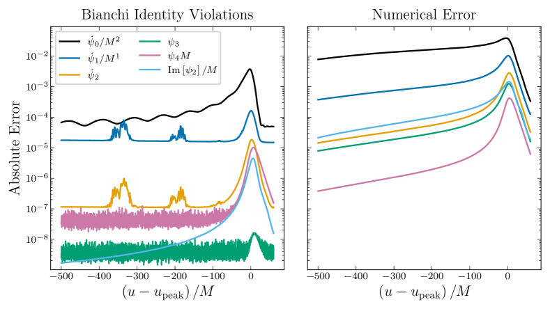
Figure 1: The absolute error of the Bianchi identity violations (left) and a conservative estimate of the numerical error (right). The violation of the Bianchi identities is computed by taking the difference of the terms on the left- and right-hand sides of Eqs. (22), while the numerical error is computed by taking the difference of the two highest-resolution simulations.

So far, we have considered Eqs. (32), (39), and (48) to be equations for the moments of the news in terms of $\psi_{0}$, $\psi_{1}$, $\psi_{2}$, and $\sigma$. However, they are best thought of as consistency conditions that must be satisfied by $\sigma$ directly, as it appears on both sides of the equation (as it appears in the definition of the moments of the news). In the case where one could determine the shear from the moment, one could then ask the following question: in each of these equations, which parts of the shear come from which terms on the right-hand side? These are what we call the “shear contributing to a moment”.

The simplest relation between the moment of the news $\mathcal{N}_{n}$ and the shear $\sigma$ is given by the case where we use the “Cauchy moments” defined above in Eq. (30). From Eq. (31), it is apparent that

$$\mathcal{N}_{n-1}(u_{1},u_{0})=\partial_{u_{1}}\mathcal{N}_{n}(u_{1},u_{0}).$$ (54)

Finally, we have that

$$\bar{\sigma}(u_{1})-\bar{\sigma}(u_{0})=\mathcal{N}_{0}(u_{1},u_{0});$$ (55)

note that, since the moments of the news depend on the derivative of $\sigma$, one cannot recover the entire $\sigma$. As such, we simply define the “shear contribution” from each term by the $n$th derivative of the corresponding term in the moment of the news.

We now consider each moment: for the zeroth moment of the news, the charge and flux contributions are the change in the mass aspect $\Delta m$ and the integral of the flux $\mathcal{F}_{0}$:

$$\begin{split}\operatorname{Re}\{\eth^{2}[\bar{\sigma}(u_{1})-\bar{\sigma}(u_{0})]\}&=\Delta m(u_{1},u_{0})\\ &\hskip 11.00008pt+\int_{u_{0}}^{u_{1}}\mathcal{F}_{0}(u)\mathrm{d}u.\end{split}$$ (56)

In contrast, for the first moment, the charge contribution to the shear is the derivative of $\Delta\hat{\psi}_{1}$, and the flux contribution is $\hat{\mathcal{F}}_{1}$ (not its integral):

$$\begin{split}\eth^{3}[\bar{\sigma}(u_{1})-\bar{\sigma}(u_{0})]&=-\frac{\partial}{\partial u_{1}}\Delta\hat{\psi}_{1}(u_{1},u_{0};u_{1})+\hat{\mathcal{F}}_{1}(u_{1})\\ &\hskip 11.00008pt+\eth\int_{u_{0}}^{u_{1}}\mathcal{F}_{0}(u)\mathrm{d}u.\end{split}$$ (57)

For the second moment, the charge contribution to the shear is the second derivative of $\Delta\hat{\psi}_{0}$, and the flux contributions are $\mathcal{F}^{\rm rad./nonrad.}_{2,1}$ and $\dot{\mathcal{F}}_{2,0}$:

$$\begin{split}\eth^{4}[\bar{\sigma}(u_{1})-\bar{\sigma}(u_{0})]&=-\frac{\partial^{2}}{\partial u_{1}^{2}}\Delta\hat{\psi}_{0}(u_{1},u_{0};u_{1})+\dot{\mathcal{F}}_{2,0}(u_{1})\\ &\hskip 11.00008pt+\mathcal{F}_{2,1}^{\rm rad.}(u_{1})+\mathcal{F}_{2,1}^{\rm nonrad.}(u_{1})\\ &\hskip 11.00008pt+\eth\hat{\mathcal{F}}_{1}(u_{1})+\eth^{2}\int_{u_{0}}^{u_{1}}\mathcal{F}_{0}(u)\mathrm{d}u.\end{split}$$ (58)

These are the quantities which we plot in Sec. IV.

Note that, in order to determine the contributions to the shear, one must invert the angular operators that act on the left-hand sides of Eqs. (32), (39), and (48), which can be easily done mode-by-mode on a basis of spin-weighted spherical harmonics using Eq. (16).

IV Results

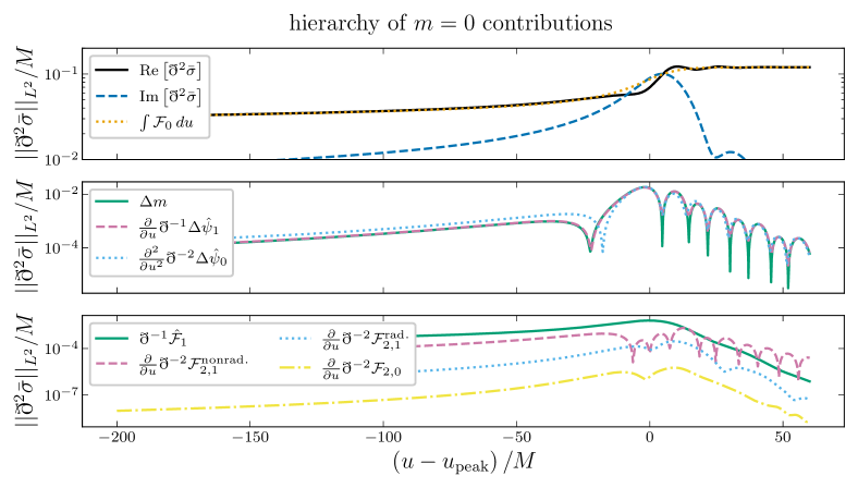
Figure 2: The $L^{2}$ norm of the $m=0$ modes of each charge and flux term’s contribution to $\eth^{2}\bar{\sigma}$, the spin-weight $0$ version of the shear. The curves are sorted by the magnitude of the time integral of their $L^{2}$ norm, that is, Eq. (60), with the largest being first. We also include the real and imaginary parts of $\eth^{2}\bar{\sigma}$ for comparison.

IV.1 Numerical Data

For our numerical analysis of the moments of the news, we examine a simulation of an equal-mass, non-spinning binary black hole system. This simulation comes from the SXS catalog and is identified by the ID SXS:BBH_ExtCCE:0001 Boyle et al. (2019). Because we are interested in not only the strain, but also the Weyl scalars at future null infinity, to perform our computations we use the waveforms that are produced by SpECTRE’s CCE module Moxon et al. (2020, 2023); Deppe et al. (2023). Last, before using the waveform and the Weyl scalars that are output by CCE, we first map this asymptotic waveform data to the post-Newtonian (PN) BMS frame using a 3PN waveform, the routine outlined in Ref. Mitman et al. (2022), and the python code scri Boyle et al. (2023); Boyle (2013); Boyle et al. (2014); Boyle (2016).

To illustrate the success of CCE at extracting the asymptotic data for this system, in Fig. 1 we show the Bianchi identity violations and an estimate of the numerical error for the asymptotic data of this system. More specifically, in the left panel we plot the $L^{2}$ norm of the difference in the right- and left-hand sides of Eqs. (22). Meanwhile, in the right panel we plot the $L^{2}$ norm of the difference of the two highest-resolution simulations, after we map the lower-resolution simulation to the BMS frame of the higher-resolution simulation Mitman et al. (2022). We define the $L^{2}$ norm of a function $f$ (over the two-sphere) as

$$||f||_{L^{2}}=\sqrt{\int f^{2}\,d\Omega}.$$ (59)

We stress that the numerical error estimate that we provide is more an error estimate on the lower-resolution simulation, and that the errors for the simulation that we examine will be smaller than what is shown. With this in mind, we find that the violation of the Bianchi identities and the numerical error for the Weyl scalars $\psi_{2}$, $\psi_{3}$, and $\psi_{4}$ are particularly low with absolute errors of $\lesssim 0.001\%$, whereas for the Weyl scalars $\psi_{0}$ and $\psi_{1}$ the Bianchi violations are noticeably larger. We attribute this to the fact that both $\psi_{0}$ and $\psi_{1}$ are more influenced by backscattering physics, that is, the fact that information should be traveling back and forth between the Cauchy evolution and CCE, than the other Weyl scalars. In fact, this notion has even been confirmed by the recent implementation of SpECTRE’s Cauchy-characteristic matching code, which shows the violation of the $\psi_{0}$ and $\psi_{1}$ Bianchi identities to be much smaller than what CCE usually yields Ma et al. (2023). Nonetheless, because the violations of the $\psi_{0}$ and $\psi_{1}$ Bianchi identities still correspond to absolute errors of $\lesssim 1\%$, the results of Fig. 1 indicate that the errors on our asymptotic data are reasonable enough to perform the following analysis. Furthermore, we find that the results drawn from the following analysis are unchanged if one uses the lower-resolution simulation instead of the higher-resolution simulation.

IV.2 Evaluation of Charges and Fluxes

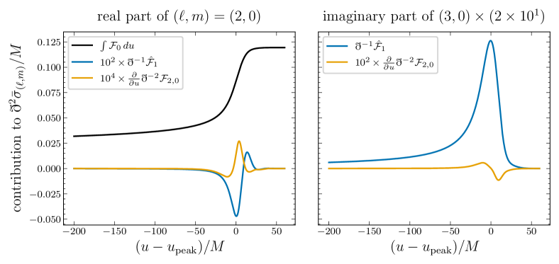
Figure 3: The flux term contributions to the real part of the $(2,0)$ mode (left) and the imaginary part of the $(3,0)$ mode (right), which represent the dominant modes for the displacement and spin memories. In these plots, we scale the $(3,0)$ mode as well as the individual flux terms by varying amounts to make their shapes easier to compare.

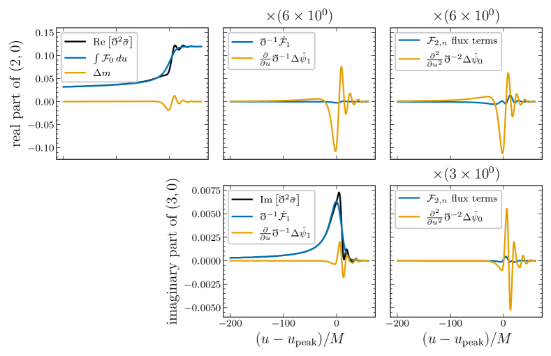
Figure 4: Contribution from the fluxes and the charges to the real part of the $(2,0)$ mode (top row) and the imaginary part of the $(3,0)$ mode (bottom row) of $\eth^{2}\bar{\sigma}$. Each column corresponds to the contribution from terms appearing in that moment of the news, e.g., the first column shows terms that appear in the balance law for the zeroth moment of the news. Certain panels are scaled by certain factors to make the comparison of each term more straightforward. For the second moment of the news, we show the sum of the $\mathcal{F}_{2,n}$ fluxes, for $n\in\{0,1\}$, since the individual fluxes are notably small.

We now illustrate the hierarchy of the various charge and flux terms in terms of their contribution to the shear for our binary black hole simulation. In Fig. 2 we show the $L^{2}$ norm of the $m=0$ modes of each term’s contribution to $\eth^{2}\bar{\sigma}$. We organize the curves that are shown in descending order with respect to the magnitude of the retarded time integral of their $L^{2}$ norms:

$$\sqrt{\int||\cdot||_{L^{2}}^{2}\mathrm{d}u}.$$ (60)

As can be seen, $\mathcal{F}_{0}$ is the largest contribution to the shear, followed by the various charge terms, and then the other flux terms, with $\hat{\mathcal{F}}_{1}$ being the second largest flux term. Note that we restrict our analysis of these terms to the $m=0$ modes because these modes are the modes which typically are the most non-oscillatory Mitman et al. (2020). Therefore, by focusing on these modes we have a better understanding of the hierarchy of the non-oscillatory contributions to the shear.

With the hierarchy of these terms understood, we now turn to examining the contributions of the flux terms to the primary non-oscillatory modes: the real part of the $(2,0)$ mode and the imaginary part of the $(3,0)$ mode. We focus on the flux terms because, for binary systems, these terms should contribute more to net changes in the various moments of the news than the charge terms, which will dominate for unbound systems. In Fig. 3 we show the contributions from $\mathcal{F}_{0}$, $\hat{\mathcal{F}}_{1}$, and $\mathcal{F}_{2,0}$ to the real part of the $(2,0)$ mode and the imaginary part of the $(3,0)$ mode of the shear. As can be seen, the $\mathcal{F}_{0}$, $\mathrm{Im}[\hat{\mathcal{F}}_{1}]$, and $\mathrm{Im}[\mathcal{F}_{2,0}]$ curves, i.e., the curves corresponding to the displacement, spin, and magnetic-parity first higher memories, exhibit morphologies that one would expect based on the moment of the news that they appear in: a step-like function, a delta-like function, and the derivative of a delta-like function. The $\mathrm{Re}[\hat{\mathcal{F}}_{1}]$ and the $\mathrm{Re}[\mathcal{F}_{2,0}]$ curves, i.e., the curves corresponding to the center-of-mass and the electric-parity first higher memory, however, instead appear to break from this “derivatives of step functions”-like behavior. We believe that the reason these terms do not exhibit the expected behavior is because of one of the following reasons. First, it could be that one simply needs to perform a correction—like the Wald-Zoupas correction discussed in Sec. III.2. Or, and perhaps more likely, it may be that there are quasi-normal mode (QNM) oscillations that are obscuring the morphology. In particular, because these flux terms are second- and third-order combinations of the shear, there could be nonlinear combinations of co-rotating and counter-rotating QNMs that yield a nontrivial, oscillatory contribution to these terms which would otherwise look like derivatives of step functions Mitman et al. (2023); Cheung et al. (2023).

Finally, in Fig. 4 we show how the nonradiative fluxes and the charges contribute to these modes. As is shown, the main observation is that beyond the curves that correspond to the displacement and the spin memories, which exhibit dominant contributions from the fluxes, the remaining curves are dominated by contributions from the charges. This is expected because of the following heuristic argument.

First, note that the total signal in Fig. 4 is predominantly non-oscillatory, for both the electric and magnetic parts of the shear. Flux contributions, similarly, seem to mostly be non-oscillatory, whereas charge contributions appear to mostly be oscillatory. By comparing Eqs. (56), (57), and (58), it is apparent that (up to angular operators) the contribution to the shear from the order $n$ charge can be written as the sum of the order $n+1$ charge and flux contributions (for a similar discussion, see Ref. Siddhant et al. ). Except for the case when these two contributions sum to the total (mostly non-oscillatory) signal, they are therefore summing to a piece which is mostly oscillatory. As such, the mostly oscillatory charge contribution of order $n+1$ must be dominant over the order $n+1$ flux contribution, and this pattern should persist for all of the higher memory effects.

V Discussion

In this work we provide straightforward expressions for the first three moments of the news (that is, the displacement, drift, and first higher memories) in terms of charges and radiative and non-radiative fluxes as well as the first numerical calculation of these terms in the context of a binary black hole merger. Besides providing a hierarchy for these terms in terms of how much they contribute to the various memory effects, we also explore how much the morphology of these contributions match “derivatives of step functions”, which is what they should resemble if one assumes that they predominantly source non-oscillatory memory effects. In particular, we find that while the $\mathcal{F}_{0}$ and $\mathcal{F}_{1}$ flux contributions to the displacement and spin memory effects resemble step- and delta-like functions, the other fluxes break from this expected behavior. A possible explanation for this, however, could simply be that to make these terms exhibit this behavior, then one must perform a correction like the Wald-Zoupas correction that is used for the first moment of the news or remove the nontrivial QNM contributions that are sourced during the ringdown phase Wald and Zoupas (2000); Flanagan and Nichols (2017); Grant et al. (2022); Mitman et al. (2023); Cheung et al. (2023).

Apart from this, we also find that these higher memory contributions are particularly small, relative to their displacement and spin memory counterparts. Specifically, the contributions to the second moment of the news tend to be roughly two orders of magnitude smaller than the contributions to the zeroth moment of the news. Consequently, while these terms are interesting from a theoretical perspective because they represent certain nonlinear features of Einstein’s equations, this means that there is little hope to observe these effects until future detectors, like LISA, come online.