Kaluza-Klein monopole with scalar hair

Abstract

We construct a new family of rotating black holes with scalar hair and a regular horizon of spherical topology, within five dimensional ($d=5$) Einstein’s gravity minimally coupled to a complex, massive scalar field doublet. These solutions represent generalizations of the Kaluza-Klein monopole found by Gross, Perry and Sorkin, with a twisted $S^{1}$ bundle over a four dimensional Minkowski spacetime being approached in the far field. The black holes are described by their mass, angular momentum, tension and a conserved Noether charge measuring the hairiness of the configurations. They are supported by rotation and have no static limit, while for vanishing horizon size, they reduce to boson stars. When performing a Kaluza-Klein reduction, the $d=5$ solutions yield a family of $d=4$ spherically symmetric dyonic black holes with gauged scalar hair. This provides a link between two seemingly unrelated mechanisms to endow a black hole with scalar hair: the $d=5$ synchronization condition between the scalar field frequency and the event horizon angular velocity results in the $d=4$ resonance condition between the scalar field frequency and the electrostatic chemical potential.

1 Introduction

The five dimensional ($d=5$) extension of Einstein’s theory of General Relativity (GR) was introduced around one century ago by Kaluza kaluza and Klein Klein:1926tv in an early attempt to unify the (then) known interactions, namely gravity and electromagnetism. In the Kaluza-Klein (KK) framework, the Universe has three non-compact spatial dimensions; one extra dimension is compact, topologically a circle and sufficiently small as to remain unobservable.

This simple idea has proven to be one of the most fruitful in theoretical physics, and the original KK model has been extended in various directions, such as including more (than one) compact extra-dimensions and starting from higher dimensional theories that are not vacuum GR, including, $e.g.$, gauge and scalar fields - see ACF for a review and a large set of original literature.

In the context of this work, a feature of the (initial) KK model is of particular interest: the existence of gravitational solitons, $i.e.$ non-singular, horizonless solutions of the vacuum Einstein field equations. While no such solutions exist in four spacetime dimensions Einstein:1943ixi ; Lichnerowicz ; Lichnerowicz1 , gravitational solitons exist in KK theory, as found in the ’80s by Gross and Perry Gross:1983hb and Sorkin Sorkin:1983ns . In the simplest case, this corresponds to a regular solution, which, from a four-dimensional perspective, describes a (gravitating) Abelian magnetic monopole, a feature which has attracted much interest.

The Gross-Perry-Sorkin (GPS) soliton is the product between the $d=4$ NUT-instanton Hawking:1976jb and a time coordinate, being asymptotically locally flat only. This defines a special type of squashed KK asymptotics, with a twisted $S^{1}$ bundle over a four dimensional Minkowski spacetime being approached in the far field. As expected, the vacuum GPS soliton possesses Black Hole (BHs) generalizations Chodos:1980df ; Dobiasch:1981vh ; Pollard:1982gj ; Gibbons:1985ac ; Wang:2006nw , with an event horizon of $S^{3}$ topology, geometrically being a squashed (rather thand round) sphere. Such solutions are essentially higher dimensional near the event horizon, but look like four-dimensional - with a compactified extra-dimension -, at large distances.

An interesting question which arises in this context concerns the validity of the ’no-hair’ conjecture Bekenstein:1996pn . In particular, do the BHs with squashed KK asymptotics allow for scalar hair? In the last decade it became clear that, at least for asymptotically flat Herdeiro:2014goa or anti-de Sitter Dias:2011at BHs, there is a generic mechanism allowing for complex scalar hair around rotating horizons. This mechanism relies on a synchronization condition Herdeiro:2014goa ; Herdeiro:2014ima which guarantees that there is no scalar energy flux crossing the horizon. Mathematically, this results in the following relation between the scalar field frequency $\omega$ and the event horizon angular velocity $\Omega_{H}$:

$$\omega=m\Omega_{H}~{},$$ (1.1)

where $m$ is the winding number which enters the scalar ansatz and $m\in\mathbb{Z}^{+}$ for the $d=4$ BHs in Herdeiro:2014goa ; Herdeiro:2014ima . Eq. (1.1) means that the scalar field phase angular velocity matches the horizon’s angular velocity; hence the name ’synchronization’. This mechanism appears to possess a certain degree of universality, applying to both asymptotically flat ($d=4$) neutral Herdeiro:2014goa and electrically charged Delgado:2016jxq rotating BHs, as well as to BHs in $d>4$ dimensions Brihaye:2014nba ; Herdeiro:2015kha , toroidal horizon topology Herdeiro:2017oyt , or AdS asymptotics Dias:2011at , and even to other spin fields Herdeiro:2016tmi ; Santos:2020pmh .

One of the main results of this work is to provide evidence that the same mechanism holds as well for BHs with the same squashed KK asymptotics as the GPS soliton. To do so, we consider $d=5$ Einstein’s gravity minimally coupled to a massive complex scalar field doublet, with a special ansatz, originally introduced in Hartmann:2010pm , which factorizes the angular dependence and reduces the problem to solving a set of ordinary differential equations (ODEs). By numerically solving the Einstein-Klein-Gordon (EKG) equations, we find a four parameter family of regular (on and outside the horizon) BHs with scalar hair and squashed KK asymptotics. The four continuous parameters are the mass $M$, the angular momentum $J$, the tension ${\cal T}$ and the Noether charge $Q$, which measures the scalar field outside the horizon. For vanishing horizon size, the solutions reduce to solitonic Boson Stars (BSs). Interestingly, some basic properties of these configurations are akin to those of the $d=4$ BSs and BHs with scalar hair Liebling:2012fv ; Herdeiro:2015gia , rather than those of the known $d=5$ asymptotically Minkowski EKG solutions Hartmann:2010pm ; Brihaye:2014nba .

We also consider the equivalent $d=4$ picture, obtained after performing a standard KK reduction for both the metric and the scalar field, as discussed $e.g.$ in Gross:1983hb . While the BSs result in $d=4$ singular configurations - similarly to the dimensional reduction of the (vacuum) GPS monopole -, the $d=5$ BHs correspond to asymptotically flat solutions of a specific $d=4$ Einstein-dilaton-Maxwell-(gauged) scalar (EdMgs) field model. They are spherically symmetric and describe gravitating dyonic BHs with scalar hair. Remarkably, the synchronization condition (1.1) in $d=5$ translates into the $d=4$ resonance condition:

$$\omega=q_{s}{\cal V},$$ (1.2)

which has been found in the study of charged (non-spinning) BHs with gauged scalar hair Hong:2019mcj ; Herdeiro:2020xmb ; Hong:2020miv ; Brihaye:2022afz . In (1.2) $q_{s}$ is the gauge coupling constant, while ${\cal V}$ is the electrostatic chemical potential, which, in the $d=5$ picture, corresponds to the event horizon angular velocity.

This paper is organized as follows. In Section 2 we present the EKG model together with a general framework, the ansatz taken - complemented by the equations in Appendix A -, and discuss the computation of global charges, together with the solutions of the Klein-Gordon equation in the probe limit. The EKG solutions with squashed KK asymptotics are discussed in Section 3, where we consider both the case of BSs and BHs. Section 4 is motivated by the observation that the GPS soliton can be taken as an intermediate state between the five dimensional Minkowski spacetime and the ’standard’ KK vacuum, $i.e.$ the direct product of four dimensional Minkowski spacetime and a circle. Therefore, in Section 4 we consider a comparison between the EKG solutions in Section 3 and those found for the other two spacetime asymptotics mentioned above. In particular, the basic properties of the KK vortices in EKG model are also discussed there for the first time in the literature. Section 5 reconsiders the results from a $d=4$ perspective and shows how the $synchronized$ $d=5$ spinning hairy BHs (HBHs) become $d=4$ $resonant$ spherically symmetric BHs with gauged scalar hair. We conclude in Section 6 with a discussion and some further remarks. A brief review of the vacuum spinning BH solution with squashed KK asymptotics Dobiasch:1981vh ; Wang:2006nw is presented in Appendix B, as well as an exact solution of the KG equation on an extremal (vacuum) BH background.

2 The framework

2.1 Action and field equations

We consider the $d=5$ Einstein’s gravity minimally coupled to a massive complex scalar field doublet $\Psi$, with action

$$\mathcal{S}=\frac{1}{4\pi G_{5}}\int_{\mathcal{M}}d^{5}x\sqrt{-g}\left[\frac{1}{4}R-\frac{1}{2}g^{ab}\left(\Psi_{,\,a}^{\dagger}\Psi_{,\,b}+\Psi_{,\,b}^{\dagger}\Psi_{,\,a}\right)-\mu^{2}\Psi^{\dagger}\Psi\right]-\frac{1}{8\pi G_{5}}\int_{\partial\mathcal{M}}d^{4}x\sqrt{-h}K,$$ (2.1)

where $\dagger$ denotes the complex transpose, $G_{5}$ is the five dimensional Newton’s constant, which will be set to unity in the numerics, $\mu$ is the scalar field mass, $h_{ij}$ is the induced metric on the boundary $\partial\mathcal{M}$ of the spacetime $\mathcal{M}$, and $K_{ij}$ is the extrinsic curvature of this boundary, with $K=K_{ij}h^{ij}$.

Variation of this action with respect to the metric and scalar field gives the EKG equations:

$$R_{ab}-\frac{1}{2}g_{ab}R=2~{}T_{ab}\,,~{}~{}\left(\Box-\mu^{2}\right)\Psi=0~{},$$ (2.2)

where

$$T_{ab}=\Psi_{,a}^{\dagger}\Psi_{,b}+\Psi_{,b}^{\dagger}\Psi_{,a}-g_{ab}\left[\frac{1}{2}g^{cd}\left(\Psi_{,c}^{\dagger}\Psi_{,d}+\Psi_{,d}^{\dagger}\Psi_{,c}\right)+\mu^{2}\Psi^{\dagger}\Psi\right]~{},$$ (2.3)

is the stress-energy tensor of the scalar field.

2.2 The vacuum Gross-Perry-Sorkin solution

We start by introducing the squashed Kaluza-Klein (KK) geometry found in Gross:1983hb ; Sorkin:1983ns , which captures some of the basic features of the solutions constructed in this work. This metric solves the vacuum Einstein equations, $\Psi=0$, and is the product between the $d=4$ (self-dual) Euclidean Taub-NUT instanton Hawking:1976jb and a time coordinate,

$$ds^{2}=-dt^{2}+ds_{4}^{2}\ .$$ (2.4)

The instanton metric $ds_{4}^{2}$ possesses an intrinsic length scale $N\geqslant 0$, which is an input parameter: the NUT charge. The geometry can be written with several different choices of the radial coordinate $r$, which make more transparent various limits of interest.

The first form for the instanton metric we shall consider is

$$ds_{4}^{2}=\frac{r+N}{r-N}dr^{2}+(r^{2}-N^{2})(d\theta^{2}+\sin^{2}\theta d\varphi^{2})+\frac{r-N}{r+N}4N^{2}(d\psi+\cos\theta d\varphi)^{2}.$$ (2.5)

The range of the radial coordinate is $N\leqslant r<\infty$, while $\theta,\,\varphi$ and $\psi$ are the usual Euler angles with ranges $0\leqslant\theta\leqslant\pi$, $0\leqslant\varphi<2\pi$, $0\leqslant\psi<4\pi$. This metric is asymptotically locally flat, in the sense that the curvature goes to zero as $r\to\infty$. The surfaces of constant $r$ are topologically $S^{3}$, although their metric is a deformed 3-sphere, with an $S^{1}$ fiber over $S^{2}$. Also, $r=N$ corresponds to the origin of the coordinates, on $\mathbb{R}^{4}$, with the size of $S^{3}$ shrinking to zero.

The coordinate transformation

$$r\to r-N$$ (2.6)

leads to an equivalent form of (2.5),

$$ds_{4}^{2}=\left(1+\frac{2N}{r}\right)\left[dr^{2}+r^{2}(d\theta^{2}+\sin^{2}\theta d\varphi^{2})\right]+\frac{4N^{2}}{1+\frac{2N}{r}}(d\psi+\cos\theta d\varphi)^{2},$$ (2.7)

but now with the usual range of the new radial coordinate, $0\leqslant r<\infty$.

The $N\to 0$ limit of the $d=4$ NUT instanton corresponds to the flat $\mathbb{R}^{3}\times S^{1}$ space. To take this limit, one defines a new coordinate

$$\psi=\frac{z}{2N}\,.$$ (2.8)

Then, as $N\to 0$, one finds the line element

$$ds^{2}=-dt^{2}+dr^{2}+r^{2}(d\theta^{2}+\sin^{2}\theta d\varphi^{2})+dz^{2}\ ,$$ (2.9)

which is the $\mathbb{M}^{1,3}\times S^{1}$ metric, with an arbitrary periodicity $L$ for the coordinate $z$.

An alternative form of the instanton metric, which shall later be employed in the construction of BSs, is obtained by taking the following coordinate transformation in (2.5)

$$r\to N+\frac{r^{2}}{8N}\,,$$ (2.10)

with the new radial coordinate ranging from zero to infinity. This result in the line element

$$ds_{4}^{2}=\left(1+\frac{r^{2}}{16N^{2}}\right)\left[dr^{2}+\frac{r^{2}}{4}(d\theta^{2}+\sin^{2}\theta d\varphi^{2})\right]+\frac{1}{4}\left(\frac{r^{2}}{1+\frac{r^{2}}{16N^{2}}}\right)(d\psi+\cos\theta d\varphi)^{2}.$$ (2.11)

Then the limit $N\to\infty$ corresponds to

$$ds=-dt^{2}+dr^{2}+\frac{r^{2}}{4}\left[d\theta^{2}+\sin^{2}d\varphi^{2}+(d\psi+\cos\theta d\varphi)^{2}\right]\ ,$$ (2.12)

which is the $d=5$ Minkowski spacetime $\mathbb{M}^{1,4}$.

As such, when varying the parameter $N$, one can consider the $d=5$ metric (2.4) as interpolating between the ’standard’ KK vacuum, $i.e.$ the direct product of $d=4$ Minkowski spacetime and a circle – the limit $N\to 0$ –, and the $d=5$ Minkowski spacetime – the limit $N\to\infty$.

As expected, the GPS soliton possesses BH generalizations, with a squashed horizon of $S^{3}$ topology and nonzero size, whose basic properties are reviewed in Appendix A.

2.3 A general ansatz

The geometries studied in this work are described by a generic line element

$$ds^{2} = -{\cal F}_{0}(r)dt^{2}+{\cal F}_{1}(r)dr^{2}+{\cal F}_{2}(r)\left(\sigma_{1}^{2}+\sigma_{2}^{2}\right)+{\cal F}_{3}(r)(\sigma_{3}-2W(r)dt)^{2}\ ,$$ (2.13)

with the left-invariant 1-forms $\sigma_{i}$ on $S^{3}$,

$$\sigma_{1}=\cos\psi d\theta+\sin\psi\sin\theta d\varphi,$$

$$\sigma_{2}=-\sin\psi d\theta+\cos\psi\sin\theta d\varphi,$$ (2.14)

$$\sigma_{3}=d\psi+\cos\theta d\varphi,$$

and $(\theta,\varphi,\psi)$ the usual Euler angles defined above, while $r$ and $t$ denote the radial and time coordinates, respectively. Apart from the Killing vector $K_{0}=\partial_{\psi}$, the line element (2.13) possesses three additional Killing vectors

$$K_{1}=\sin\varphi\partial_{\theta}\,,\quad K_{2}=-\cos\varphi\partial_{\theta}+\sin\varphi\cot\theta\partial_{\varphi}-\frac{\sin\varphi}{\sin\theta}\partial_{\psi}\,,\quad K_{3}=\partial_{\varphi}\,,$$

which obey an $SU(2)$ algebra.

Concerning the scalar sector, we shall consider a general ansatz, with

$$\Psi=\phi\left(r\right)e^{-i\omega t}\hat{\Psi}_{s}\,,\quad{\rm with}~{}~{}~{}s=0,1\,,$$ (2.16)

where

$$\hat{\Psi}_{0}=\left(\begin{array}[]{c}1\\ 0\end{array}\right)\,,\quad\hat{\Psi}_{1}=\left(\begin{array}[]{c}~{}\sin\frac{\theta}{2}~{}e^{-i\frac{\varphi}{2}}\\ \cos\frac{\theta}{2}~{}e^{i\frac{\varphi}{2}}\end{array}\right)e^{i\frac{\psi}{2}}\,.$$ (2.21)

The case $s=0$ is only compatible with a static line-element, in which case similar results are found when considering a singlet scalar field, $i.e.$ $\Psi=\phi(r)e^{-i\omega t}$. In the rotating case, we shall use instead the $s=1$ scalar ansatz, which was originally proposed in Hartmann:2010pm , albeit for a parametrization of the 3-sphere in terms of $\{\Theta,\varphi_{1},\varphi_{2}\}$ - see Eq. (2.15).

Both solitons and BHs, can be studied by using the general metric form (2.13) together with the scalar ansatz (2.16), (2.21). The corresponding expressions of the Einstein and energy-momentum tensors are given in Appendix A; the resulting EKG equations depend only on the radial variable $r$. The BHs have a regular horizon located at some $r_{H}>0$, with ${\cal F}_{0}(r_{H})=0$. For solitons, the horizon is replaced with a regular origin $r=0$, where both ${\cal F}_{2}$ and ${\cal F}_{3}$ vanish, while ${\cal F}_{0}$ and ${\cal F}_{1}$ are finite and nonzero. In both cases, the solutions share the far field asymptotics with the GPS metric (2.4), (2.5), with ${\cal F}_{0}\to 1$, ${\cal F}_{1}\to 1$, ${\cal F}_{2}\to r^{2}$, ${\cal F}_{3}\to 4N^{2}$, $W\to 0$ (and also $\phi\to 0$) as $r\to\infty$.

Finally, let us mention that the action (2.1) is invariant under the global  $U(1)$ transformation $\Psi\rightarrow e^{i\alpha}\Psi$, where $\alpha$ is a constant. This implies that the current $j^{a}=-i(\Psi^{*}\partial^{a}\Psi-\Psi\partial^{a}\Psi^{*})$ is conserved, $i.e.$ $j^{a}_{\ ;a}=0$. Therefore integrating the timelike component of this current on a spacelike slice $\Sigma$ yields a conserved quantity – the Noether charge:

$$Q=\int_{\Sigma}~{}j^{t}=32\pi^{2}\int_{r_{0}}^{\infty}dr~{}F_{2}\sqrt{\frac{F_{1}F_{3}}{F_{0}}}(\omega-W)\phi^{2},$$ (2.22)

where $r_{0}=\{0,r_{H}\}$ for solitons and BHs respectively.

2.4 The computation of global changes

Apart from the Noether charge, the solutions possess three more conserved quantities: mass $M$, angular momentum $J$ and tension ${\cal T}$, whose values are encoded in the far field form of the metric functions. Given the non-standard asymptotics of the solutions in this work, one way to compute their charges is to use the quasilocal tensor of Brown and York Brown:1992br , augmented by the counterterm formalism Kraus:1999di ; Lau:1999dp ; Mann:1999pc ; Astefanesei:2005ad . This technique, inspired by the holographic renormalization method in spacetimes with anti-de Sitter (AdS) asymptotics Henningson:1998gx ; Balasubramanian:1999re consists in adding a suitable boundary counterterm $\mathcal{S}_{\rm ct}$ to the action of the theory; thus the bulk equations of motion are not altered. $\mathcal{S}_{\rm ct}$ is built up with curvature invariants of the induced metric on the boundary, which is sent to spatial infinity after the integration. Unlike the background substraction method (see below), this procedure is intrinsic to the spacetime of interest and it is unambiguous once the counterterm is specified. In our case, however, differently from the AdS case, this method has the drawback that there is no rigorous justification for the choice of the counterterm.

In this work we shall use the counterterm proposed in Mann:2005cx to compute the mass of the KK monopole, with

$$\mathcal{S}_{\rm ct}=\frac{1}{8\pi G_{5}}\int_{\partial\mathcal{M}}d^{4}x\sqrt{-h}\sqrt{2\mathsf{R}}\,,$$ (2.23)

where $\mathsf{R}$ is the Ricci scalar of the induced metric on the boundary. The variation of this action $w.r.t.$ $h_{ij}$ results in the boundary stress-energy tensor

$$T_{ij}=\frac{1}{8\pi G_{5}}\left(K_{ij}-Kh_{ij}-\Phi(\mathsf{R}_{ij}-\mathsf{R}h_{ij})-h_{ij}h^{kl}\Phi_{;kl}+\Phi_{;ij}\right)\,,$$ (2.24)

where we defined $\Phi=\sqrt{2/{\mathsf{R}}}$. If the boundary geometry has an isometry generated by a Killing vector $\xi^{i}$, then $T_{ij}\xi^{j}$ is divergence free, from which it follows that the quantity

$$\mathcal{Q}=\int_{\Sigma}d\Sigma_{i}T^{i}{}_{j}\xi^{j},$$ (2.25)

associated with a closed surface $\Sigma$, is conserved. Physically, this means that the observers on the boundary with the induced metric $h_{ij}$ measure the same value of $\mathcal{Q}$. For the considered framework, the mass $M$, tension ${\cal T}$ and angular momentum $J$ are computed as the integrals of the boundary stress-energy tensor components $T_{t}^{t}$, $T_{\psi}^{\psi}$ and $T_{\psi}^{t}$, respectively. Interestingly, as found in Mann:2005cx , this approach predicts a non-zero value for the mass and tension of the GPS soliton (2.4), respectively

$$M=M_{0}=\frac{4\pi N^{2}}{G_{5}},~{}~{}{\cal T}={\cal T}_{0}=-\frac{N}{G_{5}}~{},$$ (2.26)

while the angular momentum is zero, as expected. When considering solutions of the EKG equations with the same asymptotics, $M$ and ${\cal T}$ will contain the above background contributions.

Apart from the boundary counterterm method, we have also computed $M,{\cal T}$ and $J$ by using the Abbott-Deser approach Abbott:1981ff . This was initially proposed to address the issue of conserved charges of asymptotically (anti-)de Sitter spacetime, but has also proved useful for other asymptotic behaviors. In this approach, conserved charges are associated with isometries of some background geometry and can be summarized as follows. First, the following decomposition of the metric is introduced

$$g_{ab}=\bar{g}_{ab}+\bar{h}_{ab}\,,$$ (2.27)

where $\bar{g}_{ab}$ corresponds to the background metric and $\bar{h}_{ab}$ is a perturbation. Assuming that $\bar{g}_{ab}$ is a vacuum solution, then the field equations can be written as:

$$R^{ab}_{L}-\frac{1}{2}\bar{g}^{ab}R_{L}=\tilde{T}^{ab}\,,$$ (2.28)

where the subscript $L$ denotes terms that are linear in the perturbation and $\tilde{T}^{ab}$ collects all higher order terms in $\bar{h}$ (the tilde serves to distinguish it from the boundary stress-energy tensor defined above for the counterterm method). It can be shown that the left-hand side of the above equation satisfies the Bianchi identity $w.r.t.$ the background metric - see $e.g.$ chap. 6 of Ortin:2004ms ; then the field equations imply:

$$\bar{\nabla}_{a}\tilde{T}^{ab}=0\,,$$ (2.29)

where the bar indicates that the covariant derivative is taken $w.r.t.$ the background metric. If $\chi$ is a Killing vector of the background geometry, the following conservation law holds:

$$\bar{\nabla}_{a}\left(\tilde{T}^{ab}\chi_{b}\right)=0\,,$$ (2.30)

which allows to define the associated conserved charge:

$$\tilde{\mathcal{Q}}=\int_{\Sigma}d\Sigma_{i}\tilde{T}^{ij}\chi_{j}\,,$$ (2.31)

where $\Sigma$ is a closed surface.

The Abbott-Deser method has been extensively used to compute conserved charges on some non-asymptotically flat spacetimes, see $e.g.$ Cai:2006td ; Wang:2006nw ; Peng:2017bjo for the case of KK asymptotics. One should, however, mention that the choice of the background metric $\bar{g}$ requires special care. It is sometimes common to consider the asymptotic metric as the background; however this is not always a solution to Einstein’s equations, in which case the effective energy-momentum tensor $\tilde{T}^{\mu\nu}$ has contributions not only from the perturbation, but also from the background. For asymptotically squashed KK spacetimes, this issue has been explored in Peng:2017bjo . The results there show that, when choosing the asymptotic form of the metric (2.4), (2.5), as the background, the mass and tension of the GPS soliton take the same (nonzero) values (2.26) as found for the counterterm approach.

The global charges of the solutions in this work were computed using both methods described above. We have found that the values of $M$, ${\cal T}$ and $J$ obtained within the counterterm approach and Abbott-Deser approach - with the asymptotic metric (2.32) taken as the reference background -, agree. But in order to simplify the picture, and in particular to make clear the limit of a vanishing scalar field, we have subtracted the $M_{0}$-term in all figures where the mass of solutions with squashed KK asymptotics is displayed, which is nonetheless in the corresponding equations.

2.5 The probe limit: no scalar clouds

Before discussing the solutions of the full system (2.2), it is of interest to consider the solutions of the KG equation in the probe-limit case, $i.e.$ ignoring the backreaction on the spacetime geometry.

Starting with the case of a GPS background as given by (2.4) and (2.5), the KG equation reads (where a prime denotes the derivative $w.r.t.$ the radial coordinate $r$):

$$\phi^{\prime\prime}+\frac{2\phi^{\prime}(r)}{r-N}+\frac{r+N}{r-N}\left(\omega^{2}-\mu_{\rm eff}^{2}\right)\phi-\frac{s(r+5N)}{8N(r-N)^{2}}\phi=0,$$ (2.33)

with $s=0,1$ for the scalar ansatz (2.16), (2.21). Also, in the above expression we define

$$\mu_{\rm eff}=\sqrt{\mu^{2}+\frac{s}{16N^{2}}}\,.$$ (2.34)

That is, for $s=1$, the scalar field acquires a contribution to the mass coming from the dependence on the $\psi$-direction, giving rise to an effective mass, a features shared also by the gravitating solutions. The bound state condition then needs to consider this effective mass, $i.e.$ $\omega^{2}\leqslant\mu_{\rm eff}^{2}$.

For the scalar Ansatz (2.16), (2.21) with $s=0$, the general solution of the equation (2.33) reads $\phi(r)=c_{1}\phi_{1}(r)+c_{2}\phi_{2}(r)$ where $c_{1},c_{2}$ are arbitrary constants, and

$$\phi_{1}(r)=\frac{N}{r-N}\mbox{e}^{-\left(r-N\right)}U\left(N\sqrt{\mu^{2}-\omega^{2}},0,2(r-N)\sqrt{\mu^{2}-\omega^{2}}\right)$$ (2.35)

$$\phi_{2}(r)=\frac{N}{r-N}\mbox{e}^{-\left(r-N\right)}L_{-N\sqrt{\mu^{2}-\omega^{2}}}^{-1}\left(2(r-N)\sqrt{\mu^{2}-\omega^{2}}\right)$$

Here $U$ is the confluent hypergeometric function and $L$ is the generalized Laguerre polynomial. For solutions satisfying the bound state condition, the function $\phi_{1}(r)$ diverges at $r=N$ while $\phi_{2}(r)$ diverges at infinity.

For the scalar ansatz (2.16), (2.21) with an explicit dependence of angular coordinates ($i.e.$ $s=1$), the general solution is $\phi(r)=c_{1}\phi_{1}(r)+c_{2}\phi_{2}(r)$ , where

$$\phi_{1}(r) =\sqrt{\frac{r}{N}-1}e^{-(r-N)\sqrt{\mu_{\rm eff}^{2}-\omega^{2}}}U\left(\frac{c}{2}3,2(r-N)\sqrt{\mu_{\rm eff}^{2}-\omega^{2}}\right)\,,$$ (2.36)

$$\phi_{2}(r) =\sqrt{\frac{r}{N}-1}e^{-(r-N)\sqrt{\mu_{\rm eff}^{2}-\omega^{2}}}L_{-\frac{c}{2}}^{2}\left(2(r-H)\sqrt{\mu_{\rm eff}^{2}-\omega^{2}}\right)$$

with $c=3+1/{(8N\sqrt{\mu_{\rm eff}^{2}-\omega^{2}})}+2N\sqrt{\mu_{\rm eff}^{2}-\omega^{2}}$, which is again divergent at $r=N$ or at infinity. Therefore we conclude that there are no scalar clouds on a GPS soliton background, a situation also found for the $\mathbb{M}^{1,3}\times S^{1}$ or $\mathbb{M}^{1,4}$ cases.

In $d=4$, (real frequency) bound states are found for a particular set of Kerr BHs. These configurations are at the threshold of the superradiant instability, the scalar field satisfying the synchronization condition (1.1) Hod:2012px ; Hod:2013zza . Inspired by this result, we have looked for scalar clouds on a spinning vacuum BH with squashed KK asymptotics, whose metric is presented in Appendix B.2, the scalar field ansatz being the case $s=1$ in (2.21). Unfortunately, in the generic, non-extremal case, the resulting equation for the scalar amplitude $\phi(r)$ could not be solved analytically. Therefore we have considered a numerical approach, employing similar methods as the ones described $e.g.$ in Benone:2014ssa . After imposing the synchronization condition, Eq. (1.1), we looked for scalar configurations which are regular on and outside the horizon and vanish at infinity. We found no indication that such solution exist, despite not being able to provide a non-existence proof. This result is also supported by the exact solutions (B.13) found for the extremal (spinning) BH background, which is displayed in Appendix B.2. Unlike the case of an extremal Kerr background in $d=4$ Hod:2012px , this solution is singular at the horizon or at infinity.

This non-existence result implies the absence of an existence line for the HBHs with squashed KK asymptotics, which would be given by the set of vacuum BH configurations allowing for scalar clouds. We mention that a similar result Cardoso:2005vk ; Kunduri:2006qa is found for for a test massive scalar field on the background of an asymptotically $\mathbb{M}^{1,4}$ Myers-Perry BHs Myers:1986un .

3 The solutions

3.1 The numerical approach

The numerical methods employed here are similar to those used in Brihaye:2014nba to study $d=5$ EKG solutions with equal-magnitude angular momenta and $\mathbb{M}^{1,4}$ asymptotics. The BH problem possesses four input parameters (we recall that $G_{5}=1$): two of them belong to a specific model – the scalar field mass $\mu$ and the NUT parameter $N$; and two specify a solution – the field frequency $\omega$ and the horizon radius $r_{H}$ (with $r_{H}=0$ for solitons). In practice, dimensionless variables and global quantities are introduced by using natural units set by the scalar field mass $\mu$, $e.g.$ $r\to r/\mu$, $\omega\to\omega/\mu$ and $N\to N\mu$, which reduce to taking $\mu=1$ in the input of the numerical code. As such, we are left with three (two) input parameters for BHs (solitons).

The system of five non-linear coupled ODEs for the metric functions and the scalar amplitude, subject to the boundary conditions described below, was solved using two different solvers. The BH solutions and a part of the BS sets were found by using a professional package based on the Newton-Raphson method schoen . In this case we have introduced a compactified coordinate $x$, where $0\leqslant x\leqslant 1$; the relation between the usual radial coordinate $r$ and $x$ being $r=(r_{H}+cx)/(1-x)$, with $c$ a suitable chosen constant, usually of order one. Typical grids used have around $800$ points, distributed equidistantly in $x$.

Most of the BSs solutions were found by using another package, which employs a collocation method for boundary-value ordinary differential equations and a damped Newton method of quasi-linearization COLSYS . The meshes here are non-equidistant and use around 300 points in the interval $0\leqslant r<r_{\rm max}$, with $r_{\rm max}$ around $10^{4}$.

We have compared a number of BS solutions constructed with these two different methods and found a very good agreement between them. In both cases, the constraint Einstein equation and the Smarr relation (3.14) have been used to test the accuracy of the results. Based on that, we estimate a typical relative error $<10^{-5}$ for the solutions reported herein. The numerical accuracy, however, decreases close to the maximal value of the frequency and also for solutions close to the center of the $(\omega,M)$-spiral - see below.

Finally, let us mention that in this work we report results for a nodeless scalar field amplitude only, although solutions with nodes exist as well.

3.2 Boson Stars

Before discussing the BH solutions, it is useful to first describe the properties of their solitonic limit, $i.e.$ of the BSs. In the numerical construction of these horizonless solutions, we have found useful to use the following metric ansatz

Figure 1: The profile of a typical static (left panel) and spinning (right panel) BS with the same input parameters.

- which can be viewed as a deformation of (2.11) -, in terms of four unknown functions $(F_{0},F_{1},F_{2},W)$:

$$ds^{2}=-e^{2F_{0}(r)}dt^{2} +e^{2F_{1}(r)}\left(1+\frac{r^{2}}{16N^{2}}\right)\bigg{[}dr^{2}+\frac{1}{4}r^{2}\left(\sigma_{1}^{2}+\sigma_{2}^{2}\right)\bigg{]}$$

$$+\frac{e^{2F_{2}(r)}}{4}\left(\frac{r^{2}}{1+\frac{r^{2}}{16N^{2}}}\right)\left(\sigma_{3}-2W(r)dt\right)^{2}\,.$$ (3.1)

Near the origin ($r=0$), the solutions possess a formal power series expansion, whose first terms are given by

$$F_{0}(r)=f_{00}^{(0)}+f_{02}^{(0)}r^{2}+\dots,~{}~{}F_{1}(r)=f_{10}^{(0)}+f_{12}^{(0)}r^{2}+\dots,~{}~{}$$ (3.2)

$$F_{2}(r)=f_{10}^{(0)}+f_{22}^{(0)}r^{2}+\dots,~{}~{}W(r)=w_{0}+w_{2}^{(0)}r^{2}+\dots,~{}~{}\phi(r)=\phi_{1}r+\phi_{3}r^{3}+\dots,~{}~{}$$

with all coefficients fixed by $f_{00}^{(0)}$, $f_{10}^{(0)}$, $f_{22}^{(0)}$, $w_{0}$ and $\phi_{1}$, $e.g.$ $f_{12}^{(0)}=-f_{22}^{(0)}-2\phi_{1}^{2}/3$.

For the far field expansion of the solutions, one finds

$$F_{0}(r)=\frac{f_{02}}{r^{2}}+\dots,~{}~{}F_{1}(r)=\frac{f_{12}}{r^{2}}+\dots,~{}~{}F_{2}(r)=-\frac{(f_{02}+f_{12})}{r^{2}}+\dots,~{}~{}$$

$$W(r)=\frac{w_{2}}{r^{2}}+\dots,~{}~{}\phi(r)=c_{1}\frac{e^{-r^{2}\sqrt{\mu^{2}_{\rm eff}-\omega^{2}}}}{r^{2}}+\dots,~{}~{}$$ (3.3)

with the parameters $f_{02}$, $f_{12}$, $w_{2}$ and $c_{1}$ being fixed by numerics.

The mass, tension and angular momentum are defined in terms of the asymptotic coefficients by (note the presence of the background terms (2.26) in $M,{\cal T}$)

$$M=\frac{4\pi}{G_{5}}\left[N^{2}+\frac{1}{8}(f_{12}-f_{02})\right],~{}{\cal T}=-\frac{1}{G}_{5}\left[N+\frac{1}{4N}(f_{12}+\frac{1}{2}f_{02})\right],~{}~{}J=\frac{2\pi N^{2}w_{2}}{G_{5}}\,.~{}~{}{~{}~{}~{}}$$ (3.4)

One can easily show that, as with BSs with other asymptotics, the Noether charge and the angular momenta of the spinning BSs are not independent quantities, with

$$Q=2J\,.$$ (3.5)

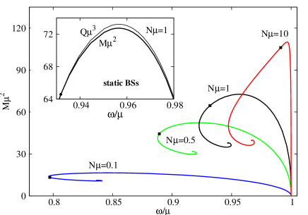
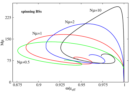
Figure 2: The frequency-mass diagram is shown for static (left panel) and spinning (right panel) families of BSs with several values of the parameter $N$. In all plots for solutions with squashed KK asymptotics shown in this work, the background contribution $M_{0}$ - $cf.$ Eq. (2.26) - is subtracted from the mass $M$, such that $M=0$ for horizonless, vacuum solutions.

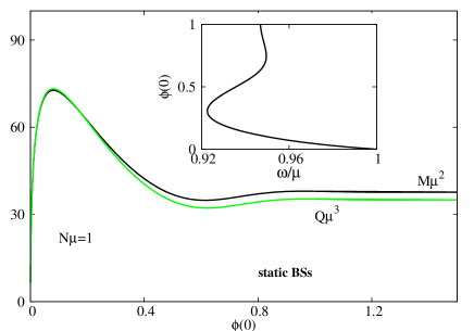
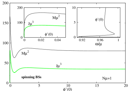
Figure 3: The mass $M$ and Noether charge $Q$ (angular momentum $J$) are shown as a function of the central value of the scalar field $\phi(0)$ (left panel, static solutions) and as a function of the first derivative of the scalar field at the origin $\phi^{\prime}(0)$ (right panel, spinning solutions). The insets shows how $\phi(0)$ (or $\phi^{\prime}(0)$) is related to the frequency parameter $\omega$.

The static solutions are constructed for a version of (3.1) with $W=0$ and $s=0$ in the scalar field ansatz (2.21). While their far field behavior is still given by (3.3), with $\mu_{\rm eff}=\mu$, the scalar field does not vanish at $r=0$, with $\phi(r)=\phi_{0}+{\cal O}(r).$

The profile of typical static and spinning BS solutions, with the same values of the input parameters $N,\mu$ and $\omega$, are shown in Figure 1. One remarks that the metric functions $F_{0},F_{1},F_{2}$ (and $W$ in the rotating case) interpolate monotonically between some constant value at the origin and zero at infinity, without presenting a local extremum.

Taking $\omega$ as a control parameter, the numerical results show that both static and spinning BSs exist for a limited range of frequencies, $\omega_{\rm min}<\omega<\mu_{\rm eff}$, with $\omega_{\rm min}$ depending on the value of the NUT parameter $N$. In the limit $\omega\rightarrow\mu_{\rm eff}$, the mass, tension and the Noether charge go to zero. One remarks that this is the behavior also found in the $d=4$ asymptotically flat case Liebling:2012fv .

As can be seen in Figure 2, the BS mass first increases as $\omega$ is decreased from $\mu_{\rm eff}$ approaching a maximal value, $M_{\rm max}$, for some $\omega_{0}$ (with both $M_{\rm max}$ and $\omega_{0}$ increasing with $N$). Then, the mass decreases, and, after some $\omega_{\rm min}$, a backbending is observed in the $M(\omega)$-diagram. Further following the curve, there is an inspiralling behaviour, towards a limiting configuration at the center of the spiral, which occurs for a frequency $\omega_{\rm cr}$ (which is also a function of $N$). This central inspiralling behaviour appears to be generic for BS solutions in EKG model, being also found in $d=4$ dimensions, or for $d=5$ solutions with $\mathbb{M}^{1,4}$ or even AdS asymptotics. A similar diagram is recovered for the curve $Q(\omega)$; for static BSs, one finds $M<\mu Q$ for a range of frequencies between $\mu$ and a critical value marked with a black dot in Figure 2 (left) (see also the inset). Rather unexpectedly, we have found that $M>\mu Q$ for all considered spinning configurations, which suggests that these solutions are unstable.

Further insights on the properties of the BSs can be taken from Figure 3, where we plot the mass $M$ and Noether charge $Q$ as a function of the central value of the scalar field $\phi(0)$ (static case) and $\phi^{\prime}(0)$ (spinning BSs). Again, one notices a rather similar picture to that found for static BSs in $d=4$ Kaup:1968zz ; Ruffini:1969qy .

3.3 Synchronized hairy Black Holes

The BH solutions are constructed for a slightly more complicated metric ansatz, which fixes the behaviour at the horizon and at infinity, and also can be taken as a deformation of the static vacuum BH (B.2), namely

$$ds^{2}=-e^{2F_{0}(r)}\frac{\left(1-\frac{r_{H}}{r}\right)^{4}}{\left(1+\frac{r_{H}}{r}\right)^{2}}dt^{2} +e^{2F_{1}(r)}H(r)\left(1+\frac{r_{H}}{r}\right)^{4}\bigg{[}dr^{2}+r^{2}\left(\sigma_{1}^{2}+\sigma_{2}^{2}\right)\bigg{]}$$

$$+e^{2F_{2}(r)}\frac{4N^{2}}{H(r)}[\sigma_{3}-2W(r)dt]^{2}\,,$$ (3.6)

with $F_{0},F_{1},F_{2}$ and $W$ resulting from numerics, and the background function

$$H(r)=1+\frac{2\left(\sqrt{N^{2}+r_{H}^{2}}-r_{H}\right)r}{(r+r_{H})^{2}}.$$ (3.7)

As with the BSs, one can write an approximate form of the solutions at the limits of the $r$-interval. The essential coefficients in these expansions determine most of the quantities of interest, either horizon quantities ($r=r_{H}$) or global quantities ($r\to\infty$). At the horizon, the Killing vector $\xi=\partial_{t}+\Omega_{H}\partial_{\psi}$ becomes null, with $\Omega_{H}=2W(r_{H})$ the event horizon angular velocity.

Figure 4: (Left panel) The metric functions $(F_{i},W)$ and the scalar field amplitude $\phi$ of a HBH solution are shown as a function of the radial coordinate. (Right panel) The metric functions $g_{tt}(r)$ and $g_{\psi\psi}(r)$ are shown for the same solution. One notices the existence of two ergo-regions ($g_{tt}>0$); also the metric function $g_{\psi\psi}(r)$ interpolates smoothly between the horizon value $g_{\psi\psi}(r_{H})=0.0076$ and the asymptotic value $g_{\psi\psi}(\infty)=4N^{2}$.

The following (formal) power series holds there (where $i=0,1,2$):

$$F_{i}(r)=f_{i0}^{(H)}+f_{i2}^{(H)}(r-r_{H})^{2}+\dots,$$

$$W(r)=\frac{1}{2}\Omega_{H}+w_{2}^{(H)}(r-r_{H})^{2}+\dots,~{}\phi(r)=\phi_{0}^{(H)}+\phi_{2}^{(H)}(r-r_{H})^{2}+\dots,~{}~{}$$ (3.8)

with the following relation between frequency and event horizon angular velocity

$$\omega=W\big{|}_{r_{H}}=\frac{1}{2}\Omega_{H}~{},$$ (3.9)

which is just the condition (1.1) with $m=1/2$, as implied by the employed scalar ansatz.

The shape of the event horizon can be read off from the induced horizon metric

$$d\Sigma_{H}^{2}=8e^{2f_{10}^{(H)}}r_{H}^{2}\Bigg{(}1+\sqrt{1+\frac{N^{2}}{r_{H}^{2}}}\,\Bigg{)}\left(\sigma_{1}^{2}+\sigma_{2}^{2}\right)+\frac{8N^{2}e^{2f_{20}^{(H)}}}{1+\sqrt{1+\frac{N^{2}}{r_{H}^{2}}}}\sigma_{3}^{2}\,,$$ (3.10)

which describes a squashed $S^{3}$ geometry. The expansions at the horizon, (3.8), can be used to compute the event horizon’s area $A_{H}$ and Hawking temperature $T_{H}$, which are given by

$$A_{H}=256\sqrt{2}\pi^{2}Nr_{H}^{2}e^{2f_{10}^{(H)}+f_{20}^{(H)}}\sqrt{1+\sqrt{1+\frac{N^{2}}{r_{H}^{2}}}}\,,~{}~{}T_{H}=\frac{1}{16\pi r_{H}}\frac{\sqrt{2}~{}e^{f_{00}^{(H)}-f_{10}^{(H)}}}{\sqrt{1+\sqrt{1+\frac{N^{2}}{r_{H}^{2}}}}}\,.\ \ \$$ (3.11)

An approximate solution can also be constructed for large $r$, with

$$F_{0}(r)=\frac{f_{01}}{r}+\dots,~{}~{}F_{1}(r)=\frac{f_{11}}{r}+\dots,~{}~{}F_{2}(r)=-\frac{f_{11}+f_{01}}{r}+\dots,~{}~{}$$

$$W(r)=\frac{w_{1}}{r}+\dots,~{}~{}~{}~{}\phi(r)=c_{1}\frac{e^{-r\sqrt{\mu^{2}_{\rm eff}-\omega^{2}}}}{r}+\dots.$$ (3.12)

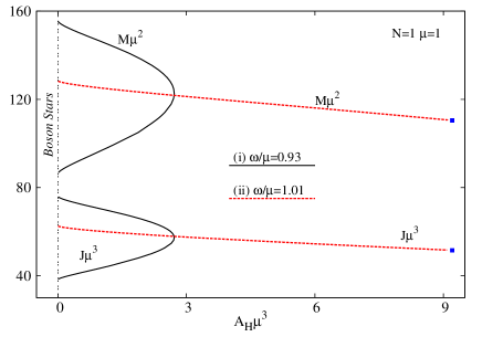
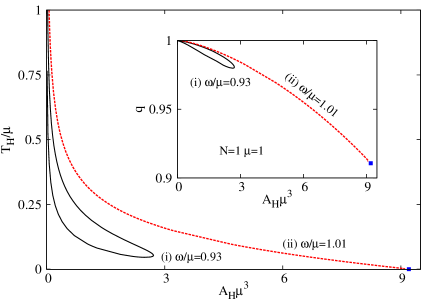
Figure 5: The mass $M$, angular momentum $J$, Hawking temperature $T_{H}$ and hairiness parameter $q=Q/(2J)$ are shown as a function of event horizon area $A_{H}$ for two sets of solutions with field frequency $\omega$ (or, equivalently, constant angular velocity $\Omega_{H}$ ). In the two cases the HBHs interpolate between a BS and $(i)$ another BS or, $(ii)$ an extremal HBH.

With these expressions, the computation of the mass, tension and angular momentum is straightforward, with

$$M=\frac{4\pi}{G_{5}}N\left(\sqrt{N^{2}+r_{H}^{2}}+3r_{H}+f_{11}-f_{01}\right),~{}~{}~{}J=\frac{16\pi N^{3}w_{1}}{G_{5}},$$ (3.13)

$${\cal T}=\frac{1}{G_{5}}\left(\sqrt{N^{2}+r_{H}^{2}}+f_{11}+\frac{1}{2}f_{01}\right).$$

As usual in BH mechanics (without a cosmological term), the temperature, horizon area and the global charges are related through a Smarr mass formula Smarr:1972kt ; Bardeen:1973gs , whose general form for the squashed KK asymptotics reads

$$M=\frac{1}{2}{\cal T}L+\frac{3}{2}T_{H}\frac{A_{H}}{4G_{5}}+\frac{3}{2}\Omega_{H}\left(J-\frac{1}{2}Q\right)+M^{(\Psi)},$$ (3.14)

where $L=8\pi N$ is the length of the twisted $S^{1}$ fiber at infinity, and

$$M^{(\Psi)}=-\frac{3}{2}\int_{\Sigma}\sqrt{-g}d^{4}x\left(T_{t}^{t}-\frac{1}{3}T_{a}^{a}\right),$$ (3.15)

is the mass stored in the matter field(s) outside the horizon.

As with other BHs with synchronized hair, to measure the ’hairiness’ of the solutions, we introduce a $normalized$ Noether charge $q$, with $q=0$ for a vanishing scalar field and $q=1$ for BSs:

$$q=\frac{Q}{2J}~{}.$$ (3.16)

The complete classification of the solutions in the space of input parameters $\{N;\omega,r_{H}\}$ is a considerable task which is beyond the scope of this paper.

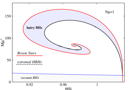
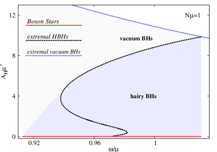
Figure 6: The domain of existence (shaded area) of HBHs is shown in a mass $vs.$ frequency (left panel) and horizon area $vs.$ frequency (right panel) plot. The vacuum, spinning BHs exist below the blue dotted line (in which case one takes $\Omega_{H}=2\omega$).

In what follows we show results for $N=1$, while a very similar phase diagram has been found for $N=0.5$, these being the only values of $N$ for which we have attempted for a systematic investigation of the solutions. However, we have also constructed HBHs with $N=0.1,~{}2$ and $5$, and the displayed picture for $N=1$ appears to be generic.

The profile of a BH solution which smoothly interpolates between the asymptotic expansions (3.8), (3.12) is shown in Figure 4. An interesting feature there is the existence of two distinct ergo-regions ($i.e.$ with $g_{tt}>0$), a feature which is found also for $d=4$ BHs with synchronized scalar hair Herdeiro:2014jaa . This is not, however, the generic behaviour, since a single ergo-region is found for a large part of the parameter space.

Given $N\neq 0$, the domain of existence of solutions is obtained by considering sequences of solutions at constant $\omega=\Omega_{H}/2$ and varying the event horizon radius $r_{H}$. As expected, a (small) BH can be added at the center of any spinning BS with a given $\omega$; this is the starting point for any aforementioned sequence. However, the end point depends on the value the frequency parameter (see Figure 5). For $\omega_{\rm min}<\omega<\omega_{i}$, the sequence ends in another BS with the same frequency (case $(i)$ in Figure 5), where we introduced $\omega_{i}$ to denote the minimum frequency possible for extremal hairy BHs, $i.e.$ the zero temperature configurations, see the black dotted curve in Figure 6. A different picture is found for $\omega_{i}<\omega<\mu_{\rm eff}$ (case $(ii)$), the sequences ending on extremal BHs with a nonvanishing horizon area and hairiness parameter $q$.

In Figure 6 (left panel), we exhibit the domain of existence of the HBHs (shaded region), in a $M(\omega)$ diagram, based on around two thousands of solution points, a similar diagram being found for $J(\omega)$. The picture possesses some similarities with the one found for spinning BHs with scalar hair in $d=4$ Herdeiro:2014goa ; Herdeiro:2015gia . As with that case, the BS curve (red solid line in Figure 6) forms a boundary of the domain; in particular the BSs set the maximal value of the BHs’ mass.

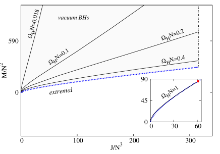
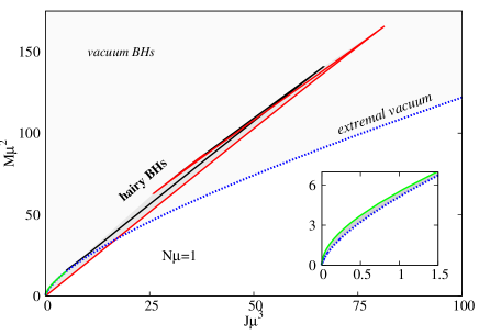
Figure 7: The mass-angular momentum diagram is shown for vacuum BHs (left panel) and for HBHs (right panel).

There is also a curve of extremal HBs (black line), which appears to inspiral towards a central value, where, we conjecture, it meets the endpoint of the BS spiral. In $d=4$, the extremal BHs curve ends in a particular vacuum Kerr solution, where it joins the existence line – a particular set of Kerr BHs allowing for scalar clouds Herdeiro:2014goa ; Herdeiro:2015gia . However, in the absence of an existence line for $d=5$ - no scalar clouds on a vacuum BH backgound -, the extremal HBH curve continues all the way to the maximal frequency, $\omega=\mu_{\rm eff}$.

Now consider the horizon area $vs.$ frequency diagram, see Figure 6 (right panel). Differently from the $d=4$ case Herdeiro:2015gia , one notices the existence there of a vertical line segment with $\omega=\mu_{\rm eff}$ and nonzero horizon area. That is, these solutions exist for a given range of $r_{H}\geqslant 0$; there the scalar field spreads and tends to zero as $\omega$ increases towards $\mu_{\rm eff}$, and also the values of the Noether charge $Q$ and of the mass stored in the field $M^{(\Psi)}$ both tend to zero. At the same time, the geometry does not trivialize, becoming that of a vacuum (spinning) KK BH, with the input parameters $\Omega_{H}=2\mu_{\rm eff}$ and $r_{H}$ (and nonzero global charges $M,{\cal T}$ and $J$).

Further insight can be found in Figure 7 (right panel), where we plot the domain of existence of HBHs in the ($J,M$)-plane Again, despite the absence of an existence line, the overall picture is rather similar to that found in Herdeiro:2015gia for the $d=4$ HBHs counterparts. Observe, however, the existence in Figure 7 (also in the inset) of a green line, which corresponds to the limiting solutions with $\omega=\mu_{\rm eff}$; this line starts at vacuum and ends in an extremal vacuum BH with (for $N\mu=1$) $M=15.0334$ and $J=4.9348$.

4 Boson stars and Black Holes with squashed Kaluza-Klein asymptotics $vs.$ solutions with $\mathbb{M}^{1,4}$ and $\mathbb{M}^{1,3}\times S^{1}$ asymptotics

One of the main goals of this work is to identify the effects of considering squashed KK asymptotics on the properties of BSs and hairy BHs solutions of the EKG system. Here we recall that, as discussed in Section 2.2, the GPS soliton - whose asymptotics provide the background of our solutions - can be seen as a vacuum state interpolating between the $\mathbb{M}^{1,4}$ and the (standard) $\mathbb{M}^{1,3}\times S^{1}$ vacua, which are approached in the limit of an infinite $N$ and vanishing $N$, respectively. As such, it is of interest to contrast the picture found above for EKG solutions with $N\neq 0$, with that for BSs and BHs solutions of the same model (2.1), which, however, approach at infinity a background given by (2.12) or (2.9). This comparison will be the main subject of this Section.

4.1 Solutions with $\mathbb{M}^{1,4}$ asymptotics

The case of EKG solutions with $\mathbb{M}^{1,4}$ asymptotics is better understood, being the subject of several studies. Starting with static, spherically symmetric solutions, we consider the scalar ansatz (2.16) and the following metric form with two functions $U(r)$ and $\delta(r)$

$$ds=-e^{-2\delta(r)}U(r)dt^{2}+\frac{dr^{2}}{U(r)}+\frac{r^{2}}{4}\left[d\theta^{2}+\sin^{2}\theta d\varphi^{2}+(d\psi+\cos\theta d\varphi)^{2}\right],$$ (4.1)

the line-element (2.12) being approached asymptotically. The horizonless solitonic solutions have been discussed in Hartmann:2010pm , describing spherically symmetric BSs, and share all basic properties of the spinning stars discussed below.

By adapting a general theorem put forward in Pena:1997cy , one can show that, as with the $d=4$ case and $\mathbb{M}^{1,3}$ asymptotics, there are no static, spherically symmetric BHs with scalar hair (here we assume the existence of an horizon with $U(r_{H})=0$ and $\delta(r_{H})$ finite). The starting point is the conservation of the energy-momentum tensor of the scalar field

$$\nabla_{a}T^{a}_{b}=0~{},$$ (4.2)

which, for $b\equiv r$ and the considered ansatz (note that we take $s=0$ in (2.21)), results in

$$e^{\delta}(e^{-\delta}T_{r}^{r})^{\prime}=-\frac{3}{r}T_{r}^{r}+\frac{1}{2}\frac{dg_{ab}}{dr}T^{ab},$$ (4.3)

with

$$T_{r}^{r}=U\phi^{\prime 2}+\left(\frac{e^{2\delta}\omega^{2}}{U}-\mu^{2}\right)\phi^{2},$$ (4.4)

and

$$\frac{1}{2}\frac{dg_{ab}}{dr}T^{ab} =$$ (4.5)

$$-\frac{3U\phi^{\prime 2}}{r} + \left(\frac{e^{2\delta}\omega^{2}}{U}-\mu^{2}\right)\frac{3\phi^{2}}{r}+\left[U\phi^{\prime 2}+\left(\mu^{2}+\frac{e^{2\delta}\omega^{2}}{U}\right)\phi^{2}\right]\delta^{\prime}-\left(\phi^{\prime 2}+\frac{e^{2\delta}\omega^{2}\phi^{2}}{U^{2}}\right)U^{\prime}.$$

However, $U^{\prime}$ and $\delta^{\prime}$ can be eliminated from the above relation by using a suitable combination of the Einstein equations, which results in the following form of Eq. (4.3)

$$e^{\delta}(e^{-\delta}T_{r}^{r})^{\prime}=-\frac{2e^{2\delta}w^{2}(1-U)\phi^{2}}{rU^{2}}-\frac{2(1+2U)\phi^{\prime 2}}{r}.$$ (4.7)

One notices that, since the $U$-equation in (4.6) implies $U<1$, the $r.h.s.$ of the above relation is a strictly negative quantity. Therefore $e^{-\delta}T_{r}^{r}$ is a strictly decreasing function. Moreover, the equation (4.7) implies the following relation (where we use the fact that the scalar field decay exponentially at infinity and thus $T^{r}_{r}\left(\infty\right)=0$):

$$T^{r}_{r}(r_{H})=e^{\delta}(r_{H})\intop_{r_{H}}^{\infty}\mathrm{d}\bar{r}\;e^{-\delta}\left(\frac{2e^{2\delta}w^{2}(1-U)\phi^{2}}{\bar{r}U^{2}}+\frac{2(1+2U)\phi^{\prime 2}}{\bar{r}}\right)\geqslant 0~{}.$$ (4.8)

To analyze the near horizon limit of Eq. (4.7), one introduces a proper radial distance $x$, which is regular at the horizon, with $dx=\frac{dr}{\sqrt{U}}$. In terms of this coordinate, the Eq. (4.7) becomes:

$$e^{\delta}\frac{d(e^{-\delta}T_{r}^{r})}{dx}=-\frac{2e^{2\delta}w^{2}(1-U)\phi^{2}}{rU^{3/2}}-\frac{2\sqrt{U}}{r}(1+2U)\phi^{\prime 2}~{}.$$ (4.9)

For regular solutions, the $r.h.s.$ of this equation should remain finite as $U\rightarrow 0$. It follows that the quantity $\frac{2e^{2\delta}w^{2}\phi^{2}}{rU^{3/2}}$ must remain finite as $r\to r_{H}$. Thus the term $\frac{e^{2\delta}\omega^{2}}{U}\phi^{2}$ will vanish in the same limit, which, from (4.4), implies $T_{r}^{r}(r_{H})\leqslant 0$. However, this would contradicts the Eq. (4.8) unless $T_{r}^{r}(r_{H})=0$. Moreover, since the integrand of the $r.h.s.$ in (4.8) has a negative sign, it follows that $\phi=0$, $i.e.$ the absence of scalar hair.

Turning to the case of the scalar field with dependence on the coordinates on the three-sphere, $i.e.$ the ansatz (2.21) with $s=1$, the corresponding spinning BSs have been discussed in Hartmann:2010pm . Their most striking property is that they do not trivialize as the maximal frequency is reached, $\omega\to\mu$ (note that this also holds for static BSs). While in this limit the scalar field spreads and tends to zero point-wise and the geometry becomes arbitrarily close to that of $\mathbb{M}^{1,4}$, the BS mass (and Noether charge/angular momentum) remains finite and nonzero in that limit, see the red curve in Fig. 8 (left panel). This implies the existence of a gap between the $\omega\to\mu$ limiting configurations and the $\phi=0$ (vacuum) $\mathbb{M}^{1,4}$ ground state. This is very different from the case of a $\mathbb{M}^{1,3}$ background, where all BS charges vanish as $\omega\to\mu$, both in the static and in the spinning cases. An analytical argument which helps to understand this different behavior was presented in Hartmann:2010pm , which we shall briefly review here. This relies on the special scaling properties of the EKG system, which are dimension dependent. Basically, as $\omega\to\mu$, the radial coordinate and the scalar field scale as $r=\tilde{r}/\xi$, $\phi=\xi^{2}\tilde{\phi}$ where $\mu^{2}=\omega^{2}+\xi^{2}\hat{w}_{c}^{2}$, with $\xi$ a small parameter and $\hat{w}_{c}$ a constant. Then, in $d=4$ the integral $\int_{0}^{\infty}dr~{}r^{2}\phi^{2}$ (which determines the Noether charge) vanishes as $\xi\to 0$, while the $d=5$ corresponding expression $\int_{0}^{\infty}dr~{}r^{3}\phi^{2}$ remains finite and nonzero. The same reasoning explains the different behavior of the scalar field mass-integral for $d=4,~{}5.$

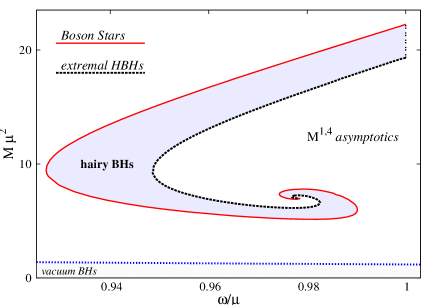
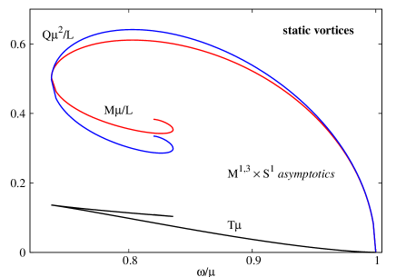
Figure 8: Left: The (frequency-mass) domain of existence of hairy BHs with $\mathbb{M}^{1,4}$ (adapted from Brihaye:2014nba ). Right: The mass, Noether charge and tension are shown as a function of frequency for EKG static vortices with $\mathbb{M}^{1,3}\times S^{1}$ asymptotics.

This argument also helps to partially understand the behavior we have found above for the BSs with squashed KK asymptotics. Since the size of $S^{3}$ in the generic ansatz (2.13) becomes proportional in the far field with $r^{2}$ only, the solutions are effectively four dimensional and thus the Noether charge integral (or the integral for the mass stored in the field) vanishes as $\omega\to\mu_{\rm eff}$.

Differently from the spherically symmetric case, the scalar field ansatz (2.21) with $s=1$ allows for hairy spinning BH solutions Brihaye:2014nba , which are found for the same ansatz employed in this work, and also obey the synchronization condition (3.9). As with the BH solutions in Section 3, the hair of the asymptotically $\mathbb{M}^{1,4}$ is intrinsically non-linear, without the existence of scalar clouds on a vacuum Myers-Perry BH background Myers:1986un ($i.e.$ of an existence line). Additionally, and naturally, the asymptotically $\mathbb{M}^{1,4}$ BH solutions inherit from the solitonic limit a gap for the mass, angular momentum and Noether charge - Fig. 8 (left panel).

4.2 The $\mathbb{M}^{1,3}\times S^{1}$ case: EKG vortices and no hairy Black Strings

To our best knowledge, the case of EKG solutions with $\mathbb{M}^{1,3}\times S^{1}$ asymptotics (see Eq. (2.9)), has not yet been considered in the literature. Such solutions, if they exist, describe EKG vortices and Black Strings.

To study them, we consider the scalar ansatz (2.16) together with the following line element

$$ds^{2}=e^{-a\psi(r)}\left(-\mbox{e}^{-2\delta(r)}U(r)dt^{2}+\frac{dr^{2}}{U(r)}+r^{2}d\Omega_{2}^{2}\right)+e^{2a\psi(r)}dz^{2}~{},$$ (4.10)

which makes contact with the $d=4$ picture discussed in the next Section, with $a=2/\sqrt{3}$ and an arbitrary periodicity $L$ for the $z$-coordinate. The metric functions $\psi(r)$, $\delta(r)$, $U(r)$, and the scalar amplitude $\phi(r)$ are solutions of the equations

$$(e^{-\delta}r^{2}U\psi^{\prime})^{\prime}+2ae^{-a\psi-\delta}\mu^{2}r^{2}\phi^{2}=0\;,~{}~{}\delta^{\prime}+r\psi^{\prime 2}+2r\left(\phi^{\prime 2}+\frac{e^{2\delta}\omega^{2}\phi^{2}}{U^{2}}\right)=0,$$

$$[r(1-U)]^{\prime}-2r^{2}\left(U\phi^{\prime 2}+(\mu^{2}e^{-a\psi})+\frac{e^{2\delta}\omega^{2}}{U}\right)\phi^{2}-r^{2}U\psi^{\prime 2}=0,$$ (4.11)

$$(e^{-\delta}r^{2}U\phi^{\prime})^{\prime}+r^{2}\left(\frac{e^{-\delta}\omega^{2}}{U}-e^{-a\psi-\delta}\mu^{2}\right)\psi=0~{}.$$

The vortices have no horizon, the size of the $S^{2}$ sector in (4.10) shrinking to zero as $r\to 0$, while the size of the $z$-circle remains finite, with $\psi(r)=\psi_{0}+{\cal O}(r^{2})$, $U(r)=1+{\cal O}(r^{2})$, $\delta(r)=\delta_{0}+{\cal O}(r^{2})$ and $\phi(r)=\phi_{0}+{\cal O}(r^{2})$ close to $r=0$ (where $\psi_{0}$, $\delta_{0}$, $\phi_{0}$ are parameters fixed by numerics). The behaviour for large-$r$ is

$$\psi=\frac{\psi_{1}}{r}+\dots,~{}U=1+\frac{h_{1}}{r}+\dots,~{}\delta=\frac{\psi_{1}^{2}}{2r^{2}}+\dots,~{}\phi=c_{1}\frac{e^{-r\sqrt{\mu^{2}-\omega^{2}}}}{r}+\dots,~{}$$ (4.12)

with the free parameters $\psi_{1}$, $h_{1}$ and $c_{1}$.

The vortices posses a nonvanishing mass, tension and Noether charge, with

$$M=-\frac{h_{1}L}{2G_{5}},~{}~{}{\cal T}=-\frac{h_{1}+3a\psi_{1}}{4G_{5}},~{}~{}Q=8\pi\omega L\int_{0}^{\infty}dr\frac{r^{2}e^{\delta}\phi^{2}}{U}~{}.$$ (4.13)

The frequency-mass diagram of these solutions is shown in Figure 8 (right panel). The picture there strongly resembles that for $d=4$ spherically symmetric BSs in the (pure) EKG model Liebling:2012fv . This can be understood by noticing that, when performing a KK reduction $w.r.t.$ the $z$-direction, these EKG vortices become $d=4$ BSs in a EKG-dilaton model - see Section 5.

As expected, no Black Strings with complex scalar hair exist in this case. This can be shown following the same Pẽna-Sudarsky-type argument Pena:1997cy as in the previous subsection. It is straightforward to show that the conservation of the stress-energy tensor together with the Einstein equations implies the following relation

$$e^{\delta+a\psi}(e^{-\delta-a\psi}T_{r}^{r})^{\prime}=-\frac{e^{2\delta+a\psi}\omega^{2}(1-U)\phi^{2}}{rU^{2}}-\frac{e^{a\psi}(1+3U)\phi^{\prime 2}}{r}-\mu^{2}r\phi^{2}\psi^{\prime 2}+a\mu^{2}\phi^{2}\psi^{\prime}.~{}~{}~{}~{}{~{}~{}~{}~{}}$$ (4.14)

Since the $\psi$-equation in (4.11) implies that $\psi^{\prime}<0$, we conclude that $T_{r}^{r}$ is a strictly decreasing function, with $T_{r}^{r}(r_{H})\geqslant 0$. However, by using similar arguments as employed above to rule out the existence of (spherically symmetric) BHs with $\mathbb{M}^{1,4}$ asymptotics, that is, by rewriting the eq. (4.14 in terms of the proper radial distance $dx=\frac{dr}{\sqrt{U}}$), one finds that $T_{r}^{r}(r_{H})\leqslant 0$. This leads to a contradiction, and we conclude that the scalar field necessarily vanishes.

The case of solutions with the $s=1$ scalar field ansatz (2.21) and $\mathbb{M}^{1,3}\times S^{1}$ asymptotics is unclear and we leave it for future studies.

5 The Kaluza-Klein reduction and the four dimensional picture

The solutions with squashed KK asymptotics in Section 3 and also the above discussed vortices can be considered from a $d=4$ perspective, upon KK reduction on a circle. Following Gross:1983hb , let us consider a generic KK metric ansatz

$$ds_{5}^{2} =e^{-a\psi(x)}ds_{4}^{2}+e^{2a\psi(x)}(dz+2A_{i}(x)dx^{i})^{2}\,,$$ (5.1)

$$\quad{\rm with}~{}~{}ds_{4}^{2}=g_{ij}^{(4)}(x)dx^{i}dx^{j}~{}~{}{\rm and}~{}~{}a=\frac{2}{\sqrt{3}},~{}{~{}~{}}$$ (5.2)

where in this section $x^{i}$ denote $d=4$ coordinates, with time $t$ being one of them, and $z$ is the (compact) fifth-dimension, which has some periodicity $L$.

For the scalar field (which can be a multiplet), one only assumes that it has a specific $z$-dependence, which disappears at the level of energy-momentum tensor and equations of motion, a single mode being excited,

$$\Psi=\Phi(x)e^{ikz},$$ (5.3)

where the function $\Phi$ can be complex, and $k=2\pi m/L$ ($m=0,\pm 1,\pm 2,\dots$).

As such, the $d=5$ EKG system admits an equivalent four dimensional description, the function $g_{zz}$ determining the dilaton $\psi$, while the metric components $g_{iz}$ resulting in a U(1) field, with the field strength tensor $F_{ij}=\partial_{i}A_{j}-\partial_{j}A_{i}$. That is, after integrating over the $z-$coordinate and dropping a boundary term, the resulting four dimensional action reads

$$\mathcal{S}_{4}=\frac{1}{4\pi G_{4}}\int_{\mathcal{M}}d^{4}x\sqrt{-g^{(4)}}\bigg{[}\frac{1}{4}R^{(4)}-\frac{1}{4}e^{3a\psi}F_{ij}F^{ij}-\frac{1}{2}\partial_{i}\psi\partial^{i}\psi$$ (5.4)

$${~{}~{}~{}~{}~{}~{}~{}~{}~{}~{}~{}~{}~{}~{}~{}~{}~{}}-\frac{1}{2}g^{ij(4)}\left(D_{i}\Phi^{\dagger}D_{j}\Phi+D_{j}\Phi^{\dagger}D_{i}\Phi\right)-U(|\Phi|,\psi\big{)}\bigg{]}~{},$$

with $G_{4}=G_{5}/L$. Observe that the $d=4$ scalar field $\Phi$ is $gauged$ $w.r.t.$ the U(1) field $A_{i}$, with the gauged derivative

$$D_{j}\Phi=(\partial_{j}-iq_{s}A_{j})\Phi,~{}~{}$$ (5.5)

the gauge coupling constant being $q_{s}=2k$ and a potential

$$U(|\Phi|,\psi)=\mu^{2}|\Phi|^{2}e^{-a\psi}+k^{2}e^{-3a\psi}|\Phi|^{2},$$ (5.6)

which depends on both $\Phi$ and $\psi$. This EdMgs model reduces to the standard KK Einstein-dilaton-Maxwell (EdM) model for $\Phi=0$. For vanishing gauge potential, $A_{i}=0$, it reduces to an Einstein-dilaton-Klein-Gordon (EdKG) model.

5.1 Static, dyonic Black Holes with gauged scalar hair

Starting with the vacuum case $(\Psi=0)$, and the squashed KK asymptotics, let us remark that, since $g_{zz}$ shrinks to zero as $r\to 0$, the dilaton diverges there and the five-dimensional GPS soliton is singular from a four dimensional perspective Gross:1983hb ; Sorkin:1983ns . However, the situation is different with BHs; for example, the spinning solution in Section B results in spherically symmetric dyonic BHs in a specific Einstein-Maxwell-dilaton model discussed $e.g.$ in Gibbons:1985ac .

Turning now to the EKG solution in Section 3, the situation with the BSs is similar to that of (vacuum) KK monopoles, being singular at $r=0$ in the $d=4$ picture. The spinning HBHs, on the other hand, result in a family of $d=4$ solutions of the model (5.4) which describe static spherically symmetric BHs with resonant gauged scalar hair and a dyonic U(1) field. All properties of these solutions follow from those of the $d=5$ EKG BHs. To make explicit this correspondence, we have found useful to consider an (equivalent) version of the $d=5$ line element with the following form of the last term in Eq. (3.6)

$$e^{2F_{2}(r)}\frac{1}{H(r)}(dz+2N\cos\theta d\varphi-4NW(r)dt)^{2},~{}~{}{\rm with}~{}~{}~{}z=2N\psi~{},$$ (5.7)

such that the dilaton $\psi(r)={F_{3}(r)}/{a}$ vanishes asymptotically. The $d=4$ gauge field describes a dyon, with $A=V(r)dt+Q_{m}\cos\theta d\varphi$, the $N$-parameter becoming in the $d=4$ perspective the magnetic charge, $Q_{m}=N$, while the $W(r)$-function associated with rotation determines the electric potential, $V(r)=-2NW(r)$. The $d=4$ BH metric reads

$$ds_{4}^{2}=-S_{0}(r)dt^{2}+S_{1}(r)\big{[}dr^{2}+r^{2}(d\theta^{2}+\sin^{2}\theta d\varphi^{2})\big{]},~{}~{}{~{}~{}}$$ (5.8)

$${\rm where}~{}~{}S_{0}(r)=e^{2F_{0}(r)+aF_{3}(r)}\frac{\left(1-\frac{r_{H}}{r}\right)^{4}}{\left(1+\frac{r_{H}}{r}\right)^{2}},~{}~{}S_{1}(r)=e^{2F_{1}(r)+aF_{3}(r)}H(r)\left(1+\frac{r_{H}}{r}\right)^{4},$$

and $H(r)$ is given by Eq. (3.7). The expression of the $d=4$ scalar field reads

$$\Phi=\phi(r)\left(\begin{array}[]{c}~{}\sin\frac{\theta}{2}~{}e^{-i\frac{\varphi}{2}}\\ \cos\frac{\theta}{2}~{}e^{i\frac{\varphi}{2}}\end{array}\right)e^{-i\omega t}.$$

The gauged coupling constant is fixed by the $N$-parameters, with $q_{s}=1/(2N)$ (and $k=1/(4N)$. Then one can easily see that $d=5$ synchronization condition (1.1) translates into the $d=4$ resonance condition (1.2), that is

$$\omega=m\Omega_{H}=W\big{|}_{r_{H}}=-\frac{1}{2N}V\big{|}_{r_{H}}=q_{s}{\cal V},$$ (5.9)

with ${\cal V}=V(\infty)-V(r_{H})$ the electrostatic chemical potential.

There is a simple map between the all quantities of interest of the $d=5$ BHs and those of the $d=4$ solutions, with $e.g.$

$$LG_{4}M^{(d=4)}=G_{5}M^{(d=5)},~{}LG_{4}Q_{e}^{(d=4)}=2G_{5}J^{(d=5)},~{}A_{H}^{(d=4)}=\frac{1}{L}A_{H}^{(d=5)},~{}T_{H}^{(d=4)}=T_{H}^{(d=5)},~{}~{}{~{}~{}~{}}$$

where $Q_{e}$ is the electric charge.

Differently from the other BHs with resonant hair discussed in the literature Hong:2019mcj ; Herdeiro:2020xmb ; Hong:2020miv ; Brihaye:2022afz , these $d=4$ solutions exist without self-interaction terms in $\Psi$, in the scalar potential (5.6). Finally, we remark that the absence of an existence line for the $d=5$ vacuum spinning BHs corresponds to the absence of charged scalar bound states on the background of a dyonic BH in a KK Einstein-dilaton-Maxwell (EdM) model, although this result should not perhaps be a surprise, given the similar findings in Hod:2012wmy ; Hod:2013nn for the Reissner-Nordström BH case.

5.2 Other cases

The case of EKG vortices with $\mathbb{M}^{1,3}\times S^{1}$ asymptotics in Section 4.2 is simpler, since the direct KK reduction leads to an (ungauged) EdKG model, $i.e.$ with $A_{i}=0$ in (5.4), while the $d=4$ metric form and dilaton are read directly from (4.10). We remark that, for the employed $s=0$ ansatz (2.16), (2.21), it is more natural to interpret the results as for a model with a single scalar field, which has the same expression (and also field mass $\mu$) in both $d=4,~{}5$.

$d=4$ solutions with a gauged scalar field can, nonetheless, be generated by using the $d=5$ EKG vortices as seeds. The basic procedure is well known in the literature - however, without also considering a complex scalar field - and works as follows. Starting with any EKG vortex, we perform a boost in the $(t,z)$-plane, with

$$\begin{cases}t=\cosh\alpha~{}T-\sinh\alpha~{}Z\\ z=\cosh\alpha~{}Z-\sinh\alpha~{}T\\ \end{cases}\,,~{}~{}{\rm where}~{}~{}\alpha\in\mathbb{R}\,.$$ (5.10)

Then a KK reduction $w.r.t.$ the direction $Z$ results in the following solution of the $d=4$ model (5.4)

$$ds_{4}^{2}=-\frac{e^{-2\delta(r)}N(r)}{\sqrt{S(r)}}dT^{2}+\sqrt{S(r)}\left(\frac{dr^{2}}{N(r)}+r^{2}d\Omega_{2}^{2}\right),~{}~{}A=V(r)dt,$$ (5.11)

where

$$S(r)=\cosh^{2}\alpha-~{}e^{-\delta(r)-3a\psi(r)}N(r)\sinh^{2}\alpha,~{}~{}V(r)=\left(e^{-2\delta(r)-3a\psi(r)}N(r)-1\right)\frac{\sinh\alpha\cosh\alpha}{2S(r)}~{},$$

while the $d=4$ dilaton field is $\psi(r)=\psi_{i}(r)+\frac{\log S(r)}{2a},$ with $\psi_{i}(r)$ the function which enters the seed $d=5$ solution, denoted by $\psi$ in the metric (4.10). The $d=4$ scalar field $\Phi$ is

$$\Phi=\phi(r)e^{-i\tilde{\omega}T},~{}~{}{\rm with}~{}~{}\tilde{\omega}=\omega\cosh\alpha,$$ (5.12)

while the gauge coupling constant is $g_{s}=2\omega\sinh\alpha$.

These solutions describe static, electrically charged, spherically symmetric gauged BSs, which are a generalisation of the usual (uncharged) EKG BSs Jetzer:1989av ; Jetzer:1992tog ; Pugliese:2013gsa , with an extra-dilaton field, $cf.$ eq. (5.4). Again, it is straightforward to derive the map between the quantities of interest of the $d=5$ and $d=4$ configurations.

Finally, we mention that the same setup can be used to construct a generalization of the known $d=4$ spherically symmetric (ungauged) BSs by including the effects of a background $U(1)$ magnetic field. In this case, one starts again with the $d=5$ EKG vortices in Section 4.2; however, the resulting $d=4$ configurations have axial symmetry only, and describe (unguged) BSs which approach asymptotically a dilatonic Melvin Universe background. The way to introduce a $d=4$ magnetic field in a KK setup involves twisting the $z$-direction Dowker:1994up ; Dowker:1995gb , that is by taking $\varphi\to\varphi+B_{0}z$ in the metric (4.10), with $B_{0}$ an arbitrary real constant, and reidentifying points appropriately. Upon reduction, the resulting $d=4$ solutions have a line element

$$ds_{4}^{2}=\sqrt{\Lambda(r,\theta)}\left(\frac{dr^{2}}{N(r)}+r^{2}d\theta^{2}-N(r)e^{-2\delta(r)}dt^{2}\right)+\frac{r^{2}\sin^{2}\theta d\varphi^{2}}{\sqrt{\Lambda(r,\theta)}},$$ (5.13)

with $\Lambda(r,\theta)=1+e^{-3a\psi(r)}B_{0}^{2}r^{2}\sin^{2}\theta$. The U(1)-potential and the $d=4$ dilaton are

$$A=\frac{e^{-3a\psi(r)}B_{0}r^{2}\sin^{2}\theta}{2\Lambda(r,\theta)}d\varphi,~{}~{}\psi(r,\theta)=\psi_{i}(r)+\frac{1}{2a}\log\Lambda(r,\theta),$$ (5.14)

while the scalar $\Phi$ has the same expression as $\Psi$ in five dimensions, and remains $ungauged$.

6 Conclusions and remarks

The study of solitons and BH solutions in more than $d=4$ dimensions is a subject of long standing interest in General Relativity, the case of a KK theory with only one (compact) extra-dimension providing the simplest model. Although the original proposal in kaluza ; Klein:1926tv does not result in a realistic theory of Nature, it still continues to provide insight into more sophisticated theories, such as supergravity and string/M-theory.

In the context of this work, we were mainly interested in KK solutions of the $d=5$ Einstein equations with a squashed sphere at infinity, the simplest case being the vacuum soliton found by Gross and Perry Gross:1983hb and Sorkin Sorkin:1983ns (GPS). As discussed by various authors, an horizon can be added also for these asymptotics, which results in BHs with a squashed horizon of $S^{3}$ topology Chodos:1980df ; Dobiasch:1981vh ; Pollard:1982gj ; Gibbons:1985ac ; Wang:2006nw .

The main purpose of this paper was to extend the solutions in Gross:1983hb ; Sorkin:1983ns ; Chodos:1980df ; Dobiasch:1981vh ; Pollard:1982gj ; Gibbons:1985ac ; Wang:2006nw by including a scalar field doublet, with a special ansatz, originally proposed in Hartmann:2010pm , in the action of the model; both solitons (BSs) and BHs were considered.

Our main results can be summarized as follows:

• We have provided evidence for the existence of BHs with scalar hair, with the same far field squashed KK asymptotics as the GPS soliton. These solutions provide further evidence for the universality of the hair synchronization mechanism. They satisfy the same specific condition between the scalar field frequency and event horizon velocity known to hold for a variety of other BHs with (complex) scalar hair, see $e.g.$ Herdeiro:2014goa -Herdeiro:2017oyt . Moreover, similar to other cases, the BHs do not trivialize in the limit of a vanishing horizon area, and become BS solutions with squashed KK asymptotics.

• The basic properties of the considered BSs and BHs are a combination between those of the known $d=4$ and $d=5$ solutions with Minkowski spacetime asymptotics. For example, as with the $d=4$ case Liebling:2012fv , the global charges of the BSs vanish as the maximal frequency is approached. On the other hand, for BHs, there is no existence line, $i.e.$ of scalar clouds on a vacuum, spinning BH background, a feature shared with the $d=5$ solutions in Ref. Brihaye:2014nba .

• As a new feature induced by the squashed KK asymptotics, the scalar field possesses (in the spinning case) an effective mass $\mu_{\rm eff}^{2}=\mu^{2}+\frac{1}{16N^{2}}$, where the second term is a geometric contribution - $N$ is related to the size of the twisted $S^{1}$ fiber at infinity. The bound state condition for the scalar field frequency is $\omega\leqslant\mu_{\rm eff}$.

• These $d=5$ solutions of the EKG equations possesses an equivalent $d=4$ description. While, as with the vacuum GPS case Gross:1983hb , the solitons corresponds to $d=4$ singular configurations, the KK reduction of the BHs result in static spherically symmetric dyonic BHs with gauged scalar hair, in a specific EdMgs model.

As a byproduct of this study, we have also investigated EKG solutions with standard $\mathbb{M}^{1,3}\times S^{1}$ asymptotics and established first the absence of static Black Strings with scalar hair. However, horizonless solutions do exist, corresponding to EKG vortices. After boosting and considering a KK reduction, these configurations result in spherically symmetric, charged BSs, generalizing for an extra-dilaton field the known gauged BSs Jetzer:1989av ; Jetzer:1992tog ; Pugliese:2013gsa . Figure 9 provides an overview of the solutions studied in this paper and their relations.

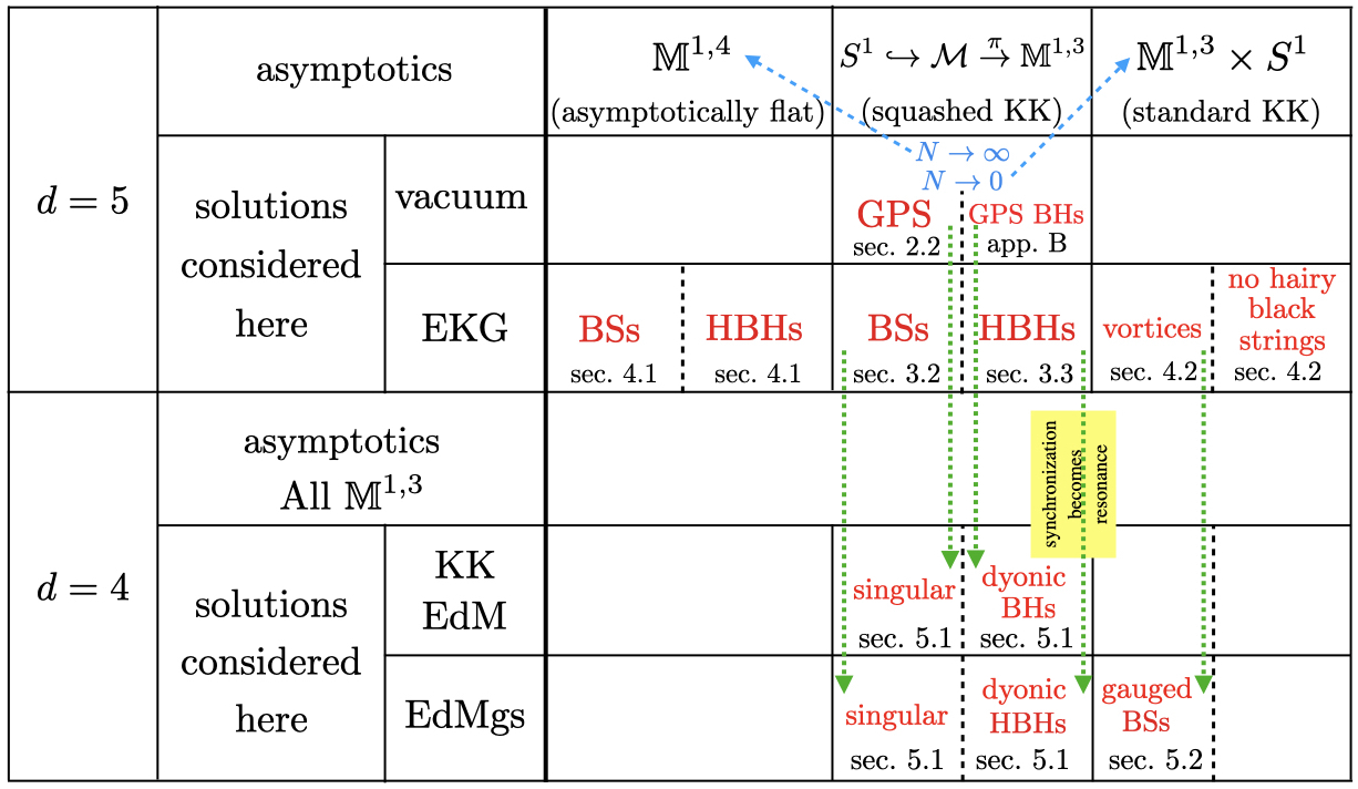
Figure 9: Overview of the solutions used or constructed in this paper and their inter-relations. The vertical green dashed arrows represent KK reduction. The sections where the solutions are discussed in this paper are also given.

As possible avenues for future research, we mention first the more systematic investigation of the $d=5$ squashed BHs solutions, such as the study of geodesic motion, their lensing properties or their thermodynamics, together with a detailed study of the resulting $d=4$ configurations. It would be interesting to investigate solutions with the same squashed KK asymptotics, but which rotate also in $\varphi$-direction, for the coordinates in the metric ansatz (2.13). This would result in EKG generalization of the vacuum BHs discussed in Rasheed:1995zv ; Matos:1996km ; Larsen:1999pp ; their study, however, requires solving a set of partial differential equations. Moreover, the KK reduction of these HBHs would result in a generalization of the $d=4$ Kerr-Newman BHs with scalar hair studied in Delgado:2016jxq , with an extra-dilaton field in the action and also with a nonzero magnetic charge.

Finally, we mention the case of KK dipolar asymptotics instead of monopolar, as in this work. In the vacuum case, such a configuration has been considered in Gross:1983hb , being again of the form (2.4), with $ds_{4}^{2}$ there corresponding to the Kerr instanton metric. We anticipate the existence of similar configurations in an EKG model with a single complex scalar field. Differently from the vacuum case, which necessarily possess a ’bolt’ - $i.e.$ a minimal nonzero size of the $S^{2}$ part in $ds_{4}^{2}$ metric -, the EKG system would allow also also for ’nutty’ solitons - that is, with the $S^{3}$ part in the $ds_{4}^{2}$ metric shrinking to zero at $r=0$, as with the BSs in this work. We hope to return elsewhere with a study of these aspects.

Appendix A The Einstein and energy-momentum tensors

To get an idea about the equations solved in practice, we display here the expression of the non-vanishing components of the Einstein tensor $E_{a}^{b}=R_{a}^{b}-\frac{1}{2}R\delta_{a}^{b}$ and of energy-momentum tensor $T_{a}^{b}$ for the generic metric ansatz (2.13) and the scalar ansatz (2.16), (2.21). For the Einstein tensor, one finds

$$E^{t}_{t} =\frac{1}{{\cal F}_{2}}\left(\frac{{\cal F}_{3}}{4{\cal F}_{2}}-1\right)+\frac{1}{{\cal F}_{1}}\left(\frac{{\cal F}_{2}^{\prime}{}^{2}}{4{\cal F}_{2}^{2}}+\frac{{\cal F}_{3}^{\prime}{}^{2}}{4{\cal F}_{3}^{2}}+\frac{{\cal F}_{1}^{\prime}{\cal F}_{2}^{\prime}}{{\cal F}_{1}F_{2}}-\frac{{\cal F}_{3}^{\prime}{\cal F}_{2}^{\prime}}{{\cal F}_{2}F_{3}}+\frac{{\cal F}_{1}^{\prime}{\cal F}_{3}^{\prime}}{2{\cal F}_{1}{\cal F}_{3}}\right)$$

$$-\frac{1}{{\cal F}_{1}}\left(\frac{2{\cal F}_{3}WW^{\prime\prime}}{{\cal F}_{0}}+\frac{{\cal F}_{2}^{\prime\prime}}{{\cal F}_{2}}+\frac{{\cal F}_{3}^{\prime\prime}}{2{\cal F}_{3}}+\frac{{\cal F}_{3}W^{\prime 2}}{{\cal F}_{0}}\right)-\frac{{\cal F}_{3}WW^{\prime}}{{\cal F}_{0}{\cal F}_{1}}\left(\frac{{\cal F}_{0}^{\prime}}{{\cal F}_{0}}+\frac{{\cal F}_{1}^{\prime}}{{\cal F}_{1}}-\frac{2{\cal F}_{2}^{\prime}}{{\cal F}_{2}}-\frac{3{\cal F}_{3}^{\prime}}{{\cal F}_{3}}\right)\,,$$

$$E_{r}^{r} =\frac{{\cal F}_{3}W^{\prime 2}}{{\cal F}_{0}{\cal F}_{1}}+\frac{1}{2{\cal F}_{1}}\left(\frac{{\cal F}_{2}^{\prime 2}}{2{\cal F}_{2}^{2}}+\frac{{\cal F}_{0}^{\prime}{\cal F}_{2}^{\prime}}{{\cal F}_{0}{\cal F}_{2}}+\frac{{\cal F}_{3}^{\prime}{\cal F}_{2}^{\prime}}{{\cal F}_{2}{\cal F}_{3}}+\frac{{\cal F}_{0}^{\prime}{\cal F}_{3}^{\prime}}{2{\cal F}_{0}{\cal F}_{3}}\right)+\frac{1}{{\cal F}_{2}}\left(\frac{F_{3}}{4{\cal F}_{2}}-1\right)\,,$$ (A.1)

$$E_{\theta}^{\theta} =E_{\varphi}^{\varphi}=(\frac{{\cal F}_{0}^{\prime\prime}}{{\cal F}_{0}}+\frac{{\cal F}_{2}^{\prime\prime}}{{\cal F}_{2}}+\frac{{\cal F}_{3}^{\prime\prime}}{{\cal F}_{3}})\frac{1}{2{\cal F}_{1}}-(\frac{{\cal F}_{0}^{\prime 2}}{{\cal F}_{0}^{2}}+\frac{{\cal F}_{2}^{\prime 2}}{{\cal F}_{2}^{2}}+\frac{{\cal F}_{3}^{\prime 2}}{{\cal F}_{3}^{2}})\frac{1}{4{\cal F}_{1}}-\frac{{\cal F}_{3}W^{\prime 2}}{{\cal F}_{0}{\cal F}_{1}}-\frac{{\cal F}_{3}}{4{\cal F}_{2}^{2}}$$

$$\qquad\qquad+(-\frac{{\cal F}_{0}^{\prime}{\cal F}_{1}^{\prime}}{{\cal F}_{0}{\cal F}_{1}}+\frac{{\cal F}_{0}^{\prime}{\cal F}_{2}^{\prime}}{{\cal F}_{0}{\cal F}_{2}}+\frac{{\cal F}_{0}^{\prime}{\cal F}_{3}^{\prime}}{{\cal F}_{0}{\cal F}_{3}}-\frac{{\cal F}_{1}^{\prime}{\cal F}_{2}^{\prime}}{{\cal F}_{1}{\cal F}_{2}}-\frac{{\cal F}_{1}^{\prime}{\cal F}_{3}^{\prime}}{{\cal F}_{1}{\cal F}_{3}}+-\frac{{\cal F}_{2}^{\prime}{\cal F}_{3}^{\prime}}{{\cal F}_{2}{\cal F}_{3}})\frac{1}{4{\cal F}_{1}},$$

$$E^{\psi}_{\psi} =\frac{1}{{\cal F}_{1}}\left(-\frac{2{\cal F}_{3}WW^{\prime\prime}}{{\cal F}_{0}}+\frac{{\cal F}_{0}^{\prime\prime}}{2{\cal F}_{0}}+\frac{{\cal F}_{2}^{\prime\prime}}{{\cal F}_{2}}\right)-\frac{1}{{\cal F}_{1}}\left(\frac{3{\cal F}_{3}W^{\prime 2}}{{\cal F}_{0}}+\frac{{\cal F}_{0}^{\prime}{}^{2}}{4{\cal F}_{0}^{2}}+\frac{{\cal F}_{2}^{\prime}{}^{2}}{4{\cal F}_{2}^{2}}\right)$$

$$\qquad+\frac{{\cal F}_{3}WW^{\prime}}{{\cal F}_{0}{\cal F}_{1}}\left(\frac{{\cal F}_{0}^{\prime}}{{\cal F}_{0}}+\frac{{\cal F}_{1}^{\prime}}{{\cal F}_{1}}-\frac{2{\cal F}_{2}^{\prime}}{{\cal F}_{2}}-\frac{3{\cal F}_{3}^{\prime}}{{\cal F}_{3}}\right)-\frac{1}{2{\cal F}_{1}}\left(\frac{{\cal F}_{0}^{\prime}{\cal F}_{1}^{\prime}}{2{\cal F}_{0}{\cal F}_{1}}+\frac{{\cal F}_{2}^{\prime}{\cal F}_{1}^{\prime}}{{\cal F}_{1}{\cal F}_{2}}-\frac{{\cal F}_{0}^{\prime}{\cal F}_{2}^{\prime}}{{\cal F}_{0}{\cal F}_{2}}\right)$$

$$\qquad+\frac{1}{{\cal F}_{2}}\left(\frac{3{\cal F}_{3}}{4{\cal F}_{2}}-1\right),$$

$$E^{t}_{\psi} =\frac{1}{\cos\theta}E^{t}_{\varphi}=\frac{W^{\prime}}{{\cal F}_{1}}\left(\frac{{\cal F}_{3}{\cal F}_{0}^{\prime}}{2{\cal F}_{0}^{2}}+\frac{{\cal F}_{3}{\cal F}_{1}^{\prime}}{2{\cal F}_{0}{\cal F}_{1}}-\frac{{\cal F}_{3}{\cal F}_{2}^{\prime}}{{\cal F}_{0}{\cal F}_{2}}-\frac{3{\cal F}_{3}^{\prime}}{2{\cal F}_{0}}\right)-\frac{{\cal F}_{3}W^{\prime\prime}}{{\cal F}_{0}{\cal F}_{1}},$$

$$E_{\varphi}^{\psi} =\cos\theta\left[\frac{1}{2{\cal F}_{1}}\left(-\frac{4{\cal F}_{3}WW^{\prime\prime}}{{\cal F}_{0}}+\frac{{\cal F}_{2}^{\prime\prime}}{F_{2}}-\frac{{\cal F}_{3}^{\prime\prime}}{{\cal F}_{3}}\right)+\frac{1}{{\cal F}_{2}}\left(\frac{{\cal F}_{3}}{{\cal F}_{2}}-1\right)\right.$$

$$\qquad\qquad\qquad+\frac{{\cal F}_{3}W^{\prime}}{{\cal F}_{1}}\left(\frac{W}{{\cal F}_{0}}\left(\frac{{\cal F}_{0}^{\prime}}{{\cal F}_{0}}+\frac{{\cal F}_{1}^{\prime}}{{\cal F}_{1}}-\frac{2{\cal F}_{2}^{\prime}}{{\cal F}_{2}}-\frac{3{\cal F}_{3}^{\prime}}{{\cal F}_{3}}\right)-\frac{2W^{\prime}}{{\cal F}_{0}}\right)$$

$$\left.\qquad\qquad\qquad+\frac{1}{4{\cal F}_{1}}\left(\frac{{\cal F}_{3}^{\prime}{}^{2}}{{\cal F}_{3}^{2}}-\frac{{\cal F}_{0}^{\prime}{\cal F}_{3}^{\prime}}{{\cal F}_{0}{\cal F}_{3}}+\frac{{\cal F}_{1}^{\prime}{\cal F}_{3}^{\prime}}{{\cal F}_{1}{\cal F}_{3}}-\frac{{\cal F}_{2}^{\prime}{\cal F}_{3}^{\prime}}{{\cal F}_{2}{\cal F}_{3}}+\frac{{\cal F}_{0}^{\prime}{\cal F}_{2}^{\prime}}{{\cal F}_{0}{\cal F}_{2}}-\frac{{\cal F}_{1}^{\prime}{\cal F}_{2}^{\prime}}{{\cal F}_{1}{\cal F}_{2}}\right)\right],$$

while the non-vanishing components of the energy momentum tensor are

$$T^{t}_{t}=-\mu^{2}\phi^{2}-\frac{\omega^{2}-sW^{2}}{{\cal F}_{0}}\phi^{2}-\frac{s}{4}\left(\frac{1}{{\cal F}_{3}}+\frac{2}{{\cal F}_{2}}\right)\phi^{2}-\frac{\phi^{\prime 2}}{F_{1}},$$

$$T_{r}^{r}=\frac{\phi^{\prime 2}}{{\cal F}_{1}}-s\frac{1}{2}(\frac{1}{{\cal F}_{2}}+\frac{1}{2{\cal F}_{3}})\phi^{2}+\frac{(\omega-sW)^{2}}{{\cal F}_{0}}\phi^{2}-\mu^{2}\phi^{2},$$

$$T_{\theta}^{\theta}=T_{\varphi}^{\varphi}=-\frac{\phi^{\prime 2}}{{\cal F}_{1}}-s\frac{1}{4{\cal F}_{3}}\phi^{2}+\frac{(\omega-sW)^{2}}{{\cal F}_{0}}\phi^{2}-\mu^{2}\phi^{2},$$

$$T_{\psi}^{\psi}=\frac{\left(\omega^{2}-pW^{2}\right)}{{\cal F}_{0}}\phi^{2}-\mu^{2}\phi^{2}+\frac{s}{4}\phi^{2}\left(\frac{1}{{\cal F}_{3}}-\frac{2}{{\cal F}_{2}}\right)-\frac{\phi^{\prime 2}}{F_{1}},$$

$$T^{t}_{\psi}=s\frac{(\omega-W)}{{\cal F}_{0}}\phi^{2},~{}~{}T^{t}_{\varphi}=T^{t}_{\psi}\cos\theta,$$ (A.2)

$$T^{\psi}_{\varphi}=s\left(\frac{2W(\omega-W)}{{\cal F}_{0}}-\frac{1}{2{\cal F}_{2}}+\frac{1}{2{\cal F}_{3}}\right)\cos\theta\;\phi^{2},$$

where $s=0,1$ – $cf.$ the scalar ansatz (2.16), (2.21).

In the numerics, we choose a metric gauge with ${\cal F}_{2}=\lambda{\cal F}_{1}r^{2}$ with $\lambda=1/4,1$ for solitons and BHs, respectively. Then $E_{\theta}^{\theta}$ is a linear combination of $E_{\psi}^{\psi}$ and $E_{\varphi}^{\psi}$ (and also for the corresponding $T_{a}^{b}$) and we are left with five Einstein equations for four metric functions. However, the $(r,r)$-Einstein equation is treated as a constraint, being satisfied once the remaining equations are zero. Therefore we conclude that the considered ansatz is consistent.

For completeness, we include here also the general equation satisfied by the scalar amplitude:

$$\phi^{\prime\prime} +\frac{1}{2}\left(\frac{{\cal F}_{0}^{\prime}}{{\cal F}_{0}}-\frac{{\cal F}_{1}^{\prime}}{{\cal F}_{1}}+\frac{2{\cal F}_{2}^{\prime}}{{\cal F}_{2}}+\frac{{\cal F}_{3}^{\prime}}{{\cal F}_{3}}\right)\phi^{\prime}$$ (A.3)

$$+\left[\frac{(\omega-sW)^{2}}{{\cal F}_{0}}-\mu^{2}-\frac{s}{2}\left(\frac{1}{{\cal F}_{2}}+\frac{1}{2{\cal F}_{3}}\right)\right]{\cal F}_{1}\phi=0.$$

Appendix B The vacuum Black Hole solution

B.1 The static Black Hole

The GPS solution allows for BH generalizations Chodos:1980df ; Dobiasch:1981vh ; Pollard:1982gj ; Gibbons:1985ac ; Wang:2006nw . The static case has a particularly simple form, with

$$ds=-\bigg{(}1-\frac{r_{h}}{r}\bigg{)}dt^{2}+\left(1+\frac{2\bar{N}}{r}\right)\left[\frac{dr^{2}}{1-\frac{r_{h}}{r}}+r^{2}(d\theta^{2}+\sin^{2}\theta d\varphi^{2})\right]+\frac{4N^{2}}{1+\frac{2\bar{N}}{r}}(d\psi+\cos\theta d\varphi)^{2}$$

with $\bar{N}=\sqrt{N^{2}+\frac{1}{16}r_{h}^{2}}-\frac{1}{4}r_{h}.$ The coordinate transformation (with $r_{h}=4r_{H})$

$$r\to r\left(1+\frac{r_{H}}{r}\right)^{2}\ ,$$ (B.1)

leads to the following equivalent form of (B.1) in isotropic coordinates, which was used as the background for the non-extremal HBH solutions reported in Section 3.3:

$$ds^{2}=-\frac{\left(1-\frac{r_{H}}{r}\right)^{4}}{\left(1+\frac{r_{H}}{r}\right)^{2}}dt^{2}+\left(1+\frac{r_{H}}{r}\right)^{4}\bigg{[}dr^{2}+r^{2}(d\theta^{2}+\sin^{2}\theta d\varphi^{2})\bigg{]}+\frac{4N^{2}}{H(r)}(d\psi+\cos\theta d\varphi)^{2}\ ,~{}~{}{~{}~{}~{}}$$ (B.2)

with the function $H(r)$ given by (3.7) and $r_{H}>0$ the event horizon radius. Note that the Schwarzschild Black String is recovered as $N\to 0$, while $r_{H}=0$ results in the GPS solution with the form (2.7) of $ds_{4}^{2}$ part of the metric. The corresponding expressions of various quantities of interest results straightforwardly from those of the spinning BHs displayed below.

B.2 The rotating Black Hole

B.2.1 The general case

The rotating generalization of the static line element (B.2) has been derived in Dobiasch:1981vh ; Wang:2006nw . It can be written in the generic form (2.13), where we have found useful to use a form of the metric functions with

$${\cal F}_{0}=\frac{(1+u^{2}(1-y))}{y}\frac{1-\frac{(1-y)P_{1}(r)}{P_{2}^{2}(r)}}{1+\frac{u^{2}(1-y)P_{1}^{2}(r)}{P_{2}^{2}(r)}}\,,\qquad{\cal F}_{1}=\frac{P_{1}(r)}{P_{2}(r)}\frac{y}{1-(1-y)\frac{P_{1}(r)}{P_{2}^{2}(r)}},~{}~{}$$

$${\cal F}_{2}=r^{2}P_{1}(r)P_{2}(r)\,,\quad{\cal F}_{3}=\frac{r_{0}^{2}\left(1+u^{2}(1-y)\frac{P_{1}^{2}(r)}{P_{2}^{2}(r)}\right)P_{2}(r)}{(1+u^{2})^{2}yP_{1}(r)}\,,$$ (B.3)

$$W(r)=\frac{(1+u^{2})^{3/2}(y-1)u}{2r_{0}\sqrt{1+(1-y)u^{2}}}\frac{1-\frac{P_{2}^{2}(r)}{P_{1}^{2}(r)}}{(y-1)u^{2}-\frac{P_{2}^{2}(r)}{P_{1}^{2}(r)}},$$

where

$$P_{1}(r)=1+\frac{r_{0}}{r},~{}~{}P_{2}(r)=1+\frac{r_{0}}{r}\frac{u^{2}}{1+u^{2}},~{}~{}$$ (B.4)

$\{r_{0},u,y\}$ being three parameters. The static limit is recovered for $u=0$, resulting in the metric form (B.1) (with $r_{h}=r_{0}(1-y)/y$ and $N=r_{0}/(2\sqrt{y})$).

Returning to the spinning case, we notice first the absence of a rotating generalization of the horizonless (vacuum) GPS soliton. To better understand the BH properties, we express the $y$-parameter in terms of the horizon radius $r_{H}$, with

$$y=\frac{r_{0}(r_{H}-(r_{0}+r_{H})u^{4})}{r_{H}(r_{0}+r_{H})(1+u^{2})^{2}}~{},$$ (B.5)

and define

$$r_{0}=sr_{H}~{}.$$ (B.6)

As such, the input parameters become $u,s$ and $r_{H}>0$, with $0\leqslant u\leqslant 1$ and $1-(1+s)u^{2}\geqslant 0$.

One can easily verify that metric has the right asymptotics, with $W\to 0$ as $r\to\infty$, while the following relation holds between the horizon radius and the NUT-parameter:

$$r_{H}=2N\left(1+u^{2}\right)\sqrt{\frac{1-(1+s)u^{4}}{s(1+s+(3+2s)u^{2}+3(1+s)u^{4}+(1+s)^{2}u^{6})}}~{}.$$ (B.7)

The computation of various quantities which enter the thermodynamic description of this rotating BH solution is straightforward, with

$$M= \frac{4\pi N^{2}}{G_{5}}\frac{\left(2+s+2(1+s)u^{2}\right)\left(1+2u^{2}+(1+s)u^{4}\right)}{\left(1+s+(3+2s)u^{2}+3(1+s)u^{4}+(1+s)^{2}u^{6}\right)^{3/2}\sqrt{s(1-(1+s)u^{4})}\ }$$

$$\times\left(1+s+(1+2s)u^{2}-(1+s)u^{4}-(1+s)^{2}u^{6}\right)\,,$$

$$J= \frac{16\pi N^{3}}{G_{5}}\sqrt{1+s}u(1+(1+s)u^{2})^{2}$$

$$\times\left(\frac{1+u^{2}}{1+s+(3+2s)u^{2}+3(1+s)u^{4}+(1+s)^{2}u^{6})}\right)^{3/2},$$

$${\cal T}= \frac{N}{2G_{5}}\frac{\left(1+s+(1+2s)u^{2}-(1+s)u^{4}-(1+s)^{2}u^{6}\right)}{\sqrt{s(1-(1+s)u^{4})}(1+s+(3+2s)u^{2}+3(1+s)u^{4}+(1+s)^{2}u^{4})^{3/2}}$$

$$\times\left(s^{2}u^{4}(u^{2}-1)+(1+u^{2})^{3}+2s(1+u^{2})(1+u^{4})\right)\,,$$

$$A_{H}= 128\pi^{2}N^{3}(1+\frac{1}{s})(1+(1+s)u^{2})^{2}(1-(1+s)u^{4})$$ (B.8)

$$\times\left(\frac{1+u^{2}}{1+s+(3+2s)u^{2}+3(1+s)u^{4}+(1+s)^{2}u^{6})}\right)^{3/2}\,,$$

$$T_{H}= \frac{1}{8\pi N}\frac{s(1-(1+s)u^{2})(1+s+(3+2s)u^{2}+3(1+s)u^{4}+(1+s)^{2}u^{6})}{(1+s)\sqrt{s(1+u^{2})}(1+(1+s)u^{2})(1-(1+s)u^{4})^{3/2}}\,,$$

$$\Omega_{H}= \frac{1}{2N}\frac{u(2+s+2(1+s)u^{2}}{1+(1+s)u^{2}}\frac{\sqrt{s}}{\sqrt{(1+s)(1+u^{2})(1-(1+s)u^{4})}}\,.$$

This solution has a variety of interesting properties, some of them different from the case of asymptotically $\mathbb{M}^{1,4}$ Myers-Perry BHs (with the same symmetries). Here we mention only the existence, for a given value of the $N$, of an upper bound of the spinning parameter $J$, with $J_{\rm max}=\frac{8\pi N^{3}}{G_{5}}$. For $J=J_{\rm max}$, the mass can take an arbitrary value $M>M_{c}=\frac{8\pi\sqrt{2}N^{2}}{G_{5}}$, see Figure 7 (left panel). Note that the solution with $M=M_{c}$, $J=J_{\rm max}$ corresponds to an extremal BH. Also, in the context of this work, it is interesting to consider the issue of solutions with constant $\Omega_{H}$. These sequences start at the horizonless GPS soliton limit; however, their end point can be different. For $0<\Omega_{H}\leqslant 1/(\sqrt{2}N)$ they reach an extremal BH solution ($T_{H}=0$) - see the inset in Figure 7 (left panel); the extremal BH is marked there with a red dot. The situation is different for larger angular velocities, and a sequence of BHs at constant $\Omega_{H}$ ends on the set of critical solutions with $J=J_{\rm max}$ and $M>M_{c}$.

B.2.2 The extremal limit and an exact solution of the Klein-Gordon equation

The extremal BH limit ($T_{H}=0$) is found for

$$s=\frac{1}{u^{2}}-1~{},$$ (B.9)

in which case the solution takes a much simpler form. One finds

$${\cal F}_{1}=\frac{\left(1-\left(1-\frac{1}{u^{2}}\right)\frac{r_{H}}{r}\right)\left(1+\frac{1-u^{2}}{1+u^{2}}\frac{r_{H}}{r}\right)}{\left(1-\frac{r_{H}}{r}\right)^{2}},~{}~{}{\cal F}_{2}=r^{2}\left(1-\left(1-\frac{1}{u^{2}}\right)\frac{r_{H}}{r}\right)\left(1+\frac{1-u^{2}}{1+u^{2}}\frac{r_{H}}{r}\right)),$$

$${\cal F}_{3}=\frac{r_{H}^{2}\left(1+\frac{2r_{H}}{r}+\frac{5r_{H}^{2}}{r^{2}}+2\left(1-\frac{r_{H}}{r}\right)\left(1+\frac{5r_{H}}{r}\right)u^{2}+5\left(1-\frac{r_{H}}{r}\right)^{2}u^{4}\right)}{u^{4}\left(1+u^{2}\right)^{2}\left(1+\frac{1-u^{2}}{1+u^{2}}\frac{r_{H}}{r}\right)\left(1-(1-\frac{1}{u^{2}}\right)\frac{r_{H}}{r})},$$ (B.10)

$$W=\frac{2u}{r}\sqrt{\frac{1+u^{2}}{1+2u^{2}+5u^{4}}}\frac{2u^{2}\left(1+u^{2}\right)+\left(1-u^{2}\right)\left(1+2u^{2}\right)\frac{r_{H}}{r}}{1+\frac{2r_{H}}{r}+\frac{5r_{H}^{2}}{r^{2}}+2\left(1-\frac{r_{H}}{r}\right)\left(1+\frac{5r_{H}}{r}\right)u^{2}+5\left(1-\frac{r_{H}}{r}\right)^{2}u^{4}}~{},$$

for the metric functions, with the main quantities of interest are

$$M=\frac{4\pi N^{2}}{G_{5}}\frac{\left(1+3u^{2}\right)^{3}}{\left(1_{2}u^{2}+5u^{4}\right)^{3/2}}\,,~{}~{}~{}J=\frac{64\pi N^{3}u^{3}}{G_{5}}\left(\frac{1+u^{2}}{1+2u^{2}+5u^{4}}\right)^{3/2}\,,$$

$$A_{H}=512\pi^{2}N^{2}u^{3}\left(\frac{1+u^{2}}{1+2u^{2}+5u^{4}}\right)^{3/2},~{}~{}~{}\Omega_{H}=\frac{1}{4N}\frac{1+3u^{2}}{u\sqrt{1+u^{2}}},$$ (B.11)

$${\cal T}=\frac{N}{G_{5}}\frac{\left(1+3u^{2}\right)\left(1+3u^{4}\right)}{\left(1+2u^{2}+5u^{4}\right)^{3/2}}.$$

The Klein-Gordon equation (A.3) (with $s=1$) takes a relatively simple form for the above (extremal) background

$$\left((r-r_{H})^{2}\phi^{\prime}\right)^{\prime}-\left(s_{2}(r-r_{H})^{2}+s_{1}(r-r_{H})+s_{0}\right)\phi=0$$ (B.12)

where we note

$$s_{0}=\frac{3}{8}+\frac{2\mu^{2}r_{H}^{2}}{u^{2}(1+u^{2})}\,,\quad s_{1}=\left(\frac{\mu^{2}r_{H}}{u^{2}(1+u^{2})}-\frac{1}{16r_{H}}\right)\left(1+3u^{2}\right)\,,~{}~{}s_{2}=\mu^{2}-\frac{u^{2}\left(1+u^{2}\right)}{16r_{H}^{2}}\,.$$

The general solution of the above equation reads

$$\phi(r)= \mbox{e}^{-\sqrt{s_{2}}(r-r_{H})}(r-r_{H})^{\frac{1}{2}\left(\sqrt{1+4s_{0}}-1\right)}$$

$$\times\bigg{[}c_{1}L_{-\kappa}^{\sqrt{4s_{0}+1}}\left(2\sqrt{s_{2}}(r-r_{H})\right)$$

$$\quad+c_{2}U\left(\kappa,1+\sqrt{1+4s_{0}},2\sqrt{s_{2}}(r-r_{H})\right)\bigg{]}$$ (B.13)

where $U$ and $L$ are the confluent hypergeometric function and the generalized Laguerre polynomial, respectively, and $\kappa=\frac{1}{2}\left(1+\sqrt{1+4s_{0}}+\frac{s_{1}}{\sqrt{s_{2}}}\right)$ ($c_{1},c_{2}$ arbitrary constants). This solution diverges either at spatial infinity or at the horizon.

References

- (1) T. Kaluza, Zum Unitätsproblem der Physik, Sitzungsber. Preuss. Akad. Wiss. Berlin (Math. Phys. ) 1921 (1921) 966 [1803.08616].
- (2) O. Klein, Quantum Theory and Five-Dimensional Theory of Relativity. (In German and English), Z. Phys. 37 (1926) 895.
- (3) T. Appelquist, A. Chodos and P.G.O. Freund, eds., Modern Kaluza-Klein theories, Frontiers in Physics, Addison-Wesley (1987).
- (4) A. Einstein and W. Pauli, On the Non-Existence of Regular Stationary Solutions of Relativistic Field Equations, Annals Math. 44 (1943) 131.
- (5) A. Lichnerowicz, Sur le charactère euclidien d’espaces-temps extérieurs statiques partout réguliers, C. R. Hebd. Seanc. Acad. Sci. 222 (1946) 432.
- (6) A. Lichnerowicz, Théories relativistes de la gravitation et de l’Eelectromagnétisme, Paris, Masson (1955).
- (7) D.J. Gross and M.J. Perry, Magnetic Monopoles in Kaluza-Klein Theories, Nucl. Phys. B 226 (1983) 29.
- (8) R.D. Sorkin, Kaluza-Klein Monopole, Phys. Rev. Lett. 51 (1983) 87.
- (9) S.W. Hawking, Gravitational Instantons, Phys. Lett. A 60 (1977) 81.
- (10) H. Ishihara and K. Matsuno, Kaluza-Klein black holes with squashed horizons, Prog. Theor. Phys. 116 (2006) 417 [hep-th/0510094].
- (11) S.S. Yazadjiev, Dilaton black holes with squashed horizons and their thermodynamics, Phys. Rev. D 74 (2006) 024022 [hep-th/0605271].
- (12) Y. Brihaye and E. Radu, Kaluza-Klein black holes with squashed horizons and d=4 superposed monopoles, Phys. Lett. B 641 (2006) 212 [hep-th/0606228].
- (13) T. Nakagawa, H. Ishihara, K. Matsuno and S. Tomizawa, Charged Rotating Kaluza-Klein Black Holes in Five Dimensions, Phys. Rev. D 77 (2008) 044040 [0801.0164].
- (14) P.G. Nedkova and S.S. Yazadjiev, New Magnetized Squashed Black Holes – Thermodynamics and Hawking Radiation, Eur. Phys. J. C 73 (2013) 2377 [1211.5249].
- (15) A. Chodos and S.L. Detweiler, Spherically Symmetric Solutions in Five-dimensional General Relativity, Gen. Rel. Grav. 14 (1982) 879.
- (16) P. Dobiasch and D. Maison, Stationary, Spherically Symmetric Solutions of Jordan’s Unified Theory of Gravity and Electromagnetism, Gen. Rel. Grav. 14 (1982) 231.
- (17) D. Pollard, Antigravity and Classical Solutions of Five-dimensional Kaluza-Klein Theory, J. Phys. A 16 (1983) 565.
- (18) G.W. Gibbons and D.L. Wiltshire, Black Holes in Kaluza-Klein Theory, Annals Phys. 167 (1986) 201.
- (19) T. Wang, A Rotating Kaluza-Klein black hole with squashed horizons, Nucl. Phys. B 756 (2006) 86 [hep-th/0605048].
- (20) J.D. Bekenstein, Black hole hair: 25 - years after, in 2nd International Sakharov Conference on Physics, pp. 216–219, 5, 1996 [gr-qc/9605059].
- (21) C.A.R. Herdeiro and E. Radu, Kerr black holes with scalar hair, Phys. Rev. Lett. 112 (2014) 221101 [1403.2757].
- (22) O.J.C. Dias, G.T. Horowitz and J.E. Santos, Black holes with only one Killing field, JHEP 07 (2011) 115 [1105.4167].
- (23) C.A.R. Herdeiro and E. Radu, A new spin on black hole hair, Int. J. Mod. Phys. D 23 (2014) 1442014 [1405.3696].
- (24) J.F.M. Delgado, C.A.R. Herdeiro, E. Radu and H. Runarsson, Kerr–Newman black holes with scalar hair, Phys. Lett. B 761 (2016) 234 [1608.00631].
- (25) Y. Brihaye, C. Herdeiro and E. Radu, Myers–Perry black holes with scalar hair and a mass gap, Phys. Lett. B 739 (2014) 1 [1408.5581].
- (26) C. Herdeiro, J. Kunz, E. Radu and B. Subagyo, Myers–Perry black holes with scalar hair and a mass gap: Unequal spins, Phys. Lett. B 748 (2015) 30 [1505.02407].
- (27) C. Herdeiro, J. Kunz, E. Radu and B. Subagyo, Probing the universality of synchronised hair around rotating black holes with Q-clouds, Phys. Lett. B 779 (2018) 151 [1712.04286].
- (28) C. Herdeiro, E. Radu and H. Rúnarsson, Kerr black holes with Proca hair, Class. Quant. Grav. 33 (2016) 154001 [1603.02687].
- (29) N.M. Santos, C.L. Benone, L.C.B. Crispino, C.A.R. Herdeiro and E. Radu, Black holes with synchronised Proca hair: linear clouds and fundamental non-linear solutions, JHEP 07 (2020) 010 [2004.09536].
- (30) B. Hartmann, B. Kleihaus, J. Kunz and M. List, Rotating Boson Stars in 5 Dimensions, Phys. Rev. D 82 (2010) 084022 [1008.3137].
- (31) S.L. Liebling and C. Palenzuela, Dynamical boson stars, Living Rev. Rel. 26 (2023) 1 [1202.5809].
- (32) C. Herdeiro and E. Radu, Construction and physical properties of Kerr black holes with scalar hair, Class. Quant. Grav. 32 (2015) 144001 [1501.04319].
- (33) J.-P. Hong, M. Suzuki and M. Yamada, Charged black holes in non-linear Q-clouds with O(3) symmetry, Phys. Lett. B 803 (2020) 135324 [1907.04982].
- (34) C.A.R. Herdeiro and E. Radu, Spherical electro-vacuum black holes with resonant, scalar -hair, Eur. Phys. J. C 80 (2020) 390 [2004.00336].
- (35) J.-P. Hong, M. Suzuki and M. Yamada, Spherically Symmetric Scalar Hair for Charged Black Holes, Phys. Rev. Lett. 125 (2020) 111104 [2004.03148].
- (36) Y. Brihaye, C. Herdeiro and E. Radu, static, charged black holes, strings and rings with resonant, scalar Q-hair, JHEP 10 (2022) 153 [2207.13114].
- (37) J.H. Traschen and D. Fox, Tension perturbations of black brane space-times, Class. Quant. Grav. 21 (2004) 289 [gr-qc/0103106].
- (38) P.K. Townsend and M. Zamaklar, The First law of black brane mechanics, Class. Quant. Grav. 18 (2001) 5269 [hep-th/0107228].
- (39) J.D. Brown and J.W. York, Jr., Quasilocal energy and conserved charges derived from the gravitational action, Phys. Rev. D 47 (1993) 1407 [gr-qc/9209012].
- (40) P. Kraus, F. Larsen and R. Siebelink, The gravitational action in asymptotically AdS and flat space-times, Nucl. Phys. B 563 (1999) 259 [hep-th/9906127].
- (41) S.R. Lau, Light cone reference for total gravitational energy, Phys. Rev. D 60 (1999) 104034 [gr-qc/9903038].
- (42) R.B. Mann, Misner string entropy, Phys. Rev. D 60 (1999) 104047 [hep-th/9903229].
- (43) D. Astefanesei and E. Radu, Quasilocal formalism and black ring thermodynamics, Phys. Rev. D 73 (2006) 044014 [hep-th/0509144].
- (44) M. Henningson and K. Skenderis, The Holographic Weyl anomaly, JHEP 07 (1998) 023 [hep-th/9806087].
- (45) V. Balasubramanian and P. Kraus, A Stress tensor for Anti-de Sitter gravity, Commun. Math. Phys. 208 (1999) 413 [hep-th/9902121].
- (46) R.B. Mann and C. Stelea, On the gravitational energy of the Kaluza Klein monopole, Phys. Lett. B 634 (2006) 531 [hep-th/0511180].
- (47) L.F. Abbott and S. Deser, Stability of Gravity with a Cosmological Constant, Nucl. Phys. B 195 (1982) 76.
- (48) T. Ortin, Gravity and strings, Cambridge Monographs on Mathematical Physics, Cambridge Univ. Press (3, 2004), 10.1017/CBO9780511616563.
- (49) R.-G. Cai, L.-M. Cao and N. Ohta, Mass and thermodynamics of Kaluza-Klein black holes with squashed horizons, Phys. Lett. B 639 (2006) 354 [hep-th/0603197].
- (50) J.-J. Peng, Revisiting the ADT mass of the five-dimensional rotating black holes with squashed horizons, Eur. Phys. J. C 77 (2017) 706.
- (51) S. Hod, Stationary Scalar Clouds Around Rotating Black Holes, Phys. Rev. D 86 (2012) 104026 [1211.3202].
- (52) S. Hod, Stationary resonances of rapidly-rotating Kerr black holes, Eur. Phys. J. C 73 (2013) 2378 [1311.5298].
- (53) C.L. Benone, L.C.B. Crispino, C. Herdeiro and E. Radu, Kerr-Newman scalar clouds, Phys. Rev. D 90 (2014) 104024 [1409.1593].
- (54) V. Cardoso and S. Yoshida, Superradiant instabilities of rotating black branes and strings, JHEP 07 (2005) 009 [hep-th/0502206].
- (55) H.K. Kunduri, J. Lucietti and H.S. Reall, Gravitational perturbations of higher dimensional rotating black holes: Tensor perturbations, Phys. Rev. D 74 (2006) 084021 [hep-th/0606076].
- (56) R.C. Myers and M.J. Perry, Black Holes in Higher Dimensional Space-Times, Annals Phys. 172 (1986) 304.
- (57) W. Schönauer and R. Weiß, The CADSOL Program Package, Universität Karlsruhe, Interner Bericht Nr. 46/92 (1992), J. Comput. Appl. Math. 27 (1989) 279.
- (58) U. Ascher, J. Christiansen and R.D. Russel, A collocation solver for mixed order systems of boundary value problems, Math. of Comp. 33 (1979) 659.
- (59) D.J. Kaup, Klein-Gordon Geon, Phys. Rev. 172 (1968) 1331.
- (60) R. Ruffini and S. Bonazzola, Systems of selfgravitating particles in general relativity and the concept of an equation of state, Phys. Rev. 187 (1969) 1767.
- (61) L. Smarr, Mass formula for Kerr black holes, Phys. Rev. Lett. 30 (1973) 71.
- (62) J.M. Bardeen, B. Carter and S.W. Hawking, The Four laws of black hole mechanics, Commun. Math. Phys. 31 (1973) 161.
- (63) C. Herdeiro and E. Radu, Ergosurfaces for Kerr black holes with scalar hair, Phys. Rev. D 89 (2014) 124018 [1406.1225].
- (64) I. Pena and D. Sudarsky, Do collapsed boson stars result in new types of black holes?, Class. Quant. Grav. 14 (1997) 3131.
- (65) C.A.R. Herdeiro, J. Kunz, I. Perapechka, E. Radu and Y. Shnir, Multipolar boson stars: macroscopic Bose-Einstein condensates akin to hydrogen orbitals, Phys. Lett. B 812 (2021) 136027 [2008.10608].
- (66) T. Harmark and N.A. Obers, New phase diagram for black holes and strings on cylinders, Class. Quant. Grav. 21 (2004) 1709 [hep-th/0309116].
- (67) T. Harmark and N.A. Obers, General definition of gravitational tension, JHEP 05 (2004) 043 [hep-th/0403103].
- (68) R. Gervalle and M.S. Volkov, Electroweak monopoles and their stability, Nucl. Phys. B 984 (2022) 115937 [2203.16590].
- (69) R. Gervalle and M.S. Volkov, Electroweak multi-monopoles, Nucl. Phys. B 987 (2023) 116112 [2211.04875].
- (70) S. Hod, Stability of the extremal Reissner-Nordstroem black hole to charged scalar perturbations, Phys. Lett. B 713 (2012) 505 [1304.6474].
- (71) S. Hod, No-bomb theorem for charged Reissner-Nordstroem black holes, Phys. Lett. B 718 (2013) 1489.
- (72) P. Jetzer and J.J. van der Bij, CHARGED BOSON STARS, Phys. Lett. B 227 (1989) 341.
- (73) P. Jetzer, P. Liljenberg and B.S. Skagerstam, Charged boson stars and vacuum instabilities, Astropart. Phys. 1 (1993) 429 [astro-ph/9305014].
- (74) D. Pugliese, H. Quevedo, J.A. Rueda H. and R. Ruffini, On charged boson stars, Phys. Rev. D 88 (2013) 024053 [1305.4241].
- (75) F. Dowker, J.P. Gauntlett, S.B. Giddings and G.T. Horowitz, On pair creation of extremal black holes and Kaluza-Klein monopoles, Phys. Rev. D 50 (1994) 2662 [hep-th/9312172].
- (76) F. Dowker, J.P. Gauntlett, G.W. Gibbons and G.T. Horowitz, The Decay of magnetic fields in Kaluza-Klein theory, Phys. Rev. D 52 (1995) 6929 [hep-th/9507143].
- (77) D. Rasheed, The Rotating dyonic black holes of Kaluza-Klein theory, Nucl. Phys. B 454 (1995) 379 [hep-th/9505038].
- (78) T. Matos and C. Mora, Stationary dilatons with arbitrary electromagnetic field, Class. Quant. Grav. 14 (1997) 2331 [hep-th/9610013].
- (79) F. Larsen, Rotating Kaluza-Klein black holes, Nucl. Phys. B 575 (2000) 211 [hep-th/9909102].
- (80) S. Tomizawa and A. Ishibashi, Charged Black Holes in a Rotating Gross-Perry-Sorkin Monopole Background, Class. Quant. Grav. 25 (2008) 245007 [0807.1564].