Wormholes and surface defects in rational ensemble holography

Abstract

We study wormhole contributions to the bulk path integral in holographic models which are dual to ensembles of rational free boson conformal field theories. We focus on the path integral on a geometry connecting two toroidal boundaries, which should capture the variance of the ensemble distribution. We show that this requirement leads to a nontrivial set of constraints which generically picks out the uniform, maximum entropy, ensemble distribution. Furthermore, we show that the two-boundary path integral should receive contributions from ‘exotic’ wormholes, which arise from the inclusion of topological surface defects.

1 Introduction and summary

Recent developments have led to a revived interest in the role of wormhole geometries contributing to the Euclidean path integral in gravity. On one hand, inclusion of replica wormholes in the path integral for the entanglement entropy of black hole radiation have shed light on the information puzzle Penington:2019kki ; Almheiri:2019qdq . On the other hand, contributions from wormholes connecting different asymptotic boundaries lead to non-factorizing observables and are a sign that the path integral computes an average over an ensemble of CFTs.

Perhaps the most clear-cut instance of such ensemble holography is that of JT gravity, where the contribution of the ‘double-trumpet’ wormhole and its generalizations are directly related to the fact that the model is dual to an ensemble of quantum mechanical theories Saad:2019lba . These insights from two-dimensional gravity have also led to a tentative reinterpretation of Maloney and Witten’s result Maloney:2007ud for the partition function of pure three dimensional anti-de Sitter gravity, which displays features of an ensemble average. For one, the resulting continuous spectrum is most naturally interpreted as describing an average of theories with discrete spectra. Furthermore, Cotler and Jensen found an explicit bulk wormhole contributing to the two-boundary partition function Cotler:2020ugk . The putative ensemble interpretation of the Maloney-Witten result for the gravity path integral on a solid torus with boundary complex structure $\tau$ would imply an identity of the form

$$\sum_{\gamma\in\Gamma/\Gamma_{f}}\left|\chi_{\rm 0}(\gamma\tau)\right|^{2}\stackrel{{\scriptstyle\mathclap{\mbox{?}}}}{{=}}\langle Z[\tau]\rangle$$ (1)

Here, the left hand side is a so-called Poincaré sum with $\chi_{\rm 0}$ Virasoro vacuum character, $\Gamma=PSL(2,\mathbb{Z})$ is the modular group and $\Gamma_{f}$ is the subgroup leaving $|\chi_{0}|^{2}$ invariant. The expectation value of the CFT partition function $Z[\tau]$ on the right-hand side stands for an ensemble average over all Virasoro CFTs. Since we have at present no control over this ensemble (nor how to define an integration measure to average over it), making (1) more precise remains a daunting task.

It is encouraging however that relations of the type (1) do turn out to hold in situations with enhanced symmetry. That is, if we replace $\chi_{\rm 0}$ by the vacuum character of an extended chiral algebra for which we have control over the moduli space of CFTs, (1) can often be turned into a mathematical identity. The candidate bulk theory giving rise to (1) is then an ‘exotic Chern-Simons gravity’, where one starts from a Chern-Simons theory realizing the appropriate chiral algebra, and supplements it with a prescription to sum over certain topologies in the path integral.

A prime example is the case where $\chi_{0}$ is taken to be the vacuum character of a $u(1)^{D}$ current algebra Afkhami-Jeddi:2020ezh ; Maloney:2020nni . Here, the Siegel-Weyl formula is an identity of the form (1) where the right hand side is an average over Narain moduli space of free boson CFTs with respect to a natural measure. Further studies and extensions of Narain holography include Perez:2020klz ; Dymarsky:2020pzc ; Datta:2021ftn ; Benjamin:2021wzr ; Ashwinkumar:2021kav ; Dong:2021wot ; Collier:2021rsn ; Benjamin:2021ygh ; Dymarsky:2021xfc ; Chakraborty:2021gzh ; Henriksson:2022dnu ; Kawabata:2022jxt ; Kames-King:2023fpa ; Alam:2023qac ; Kawabata:2023usr ; Kawabata:2023iss ; Aharony:2023zit ; Ashwinkumar:2023ctt .

As we already mentioned, the lack of factorization of ensemble-averaged two-boundary CFT partition function can be interpreted in the bulk in terms of wormhole contributions to the path integral where the boundaries are connected through the bulk. The wormhole contribution $Z_{\rm wh}[\tau_{1},\tau_{2}]$ is the connected part of the expectation value of the product of two partition functions

$$Z_{\rm conn}^{(2)}[\tau_{1},\tau_{2}] = \langle Z[\tau_{1}]Z[\tau_{2}]\rangle-\langle Z[\tau_{1}]\rangle\langle Z[\tau_{2}]\rangle$$ (2)

$$= \langle\left(Z[\tau_{1}]-\langle Z[\tau_{1}]\rangle\right)\left(Z[\tau_{2}]-\langle Z[\tau_{2}]\rangle\right)\rangle,$$

and, as rewritten in the second line, measures the variance of the ensemble distribution. The bulk interpretation of this expression however leads to a puzzle which was pointed out in Collier:2021rsn and which inspired our investigations. The authors of Collier:2021rsn computed the right hand side of (2) in the Narain ensemble and compared it to Cotler and Jensen’s direct computation Cotler:2020ugk from the path integral on a wormhole geometry. While this direct computation captures part of the result, other terms in the ensemble expression are not accounted for. It therefore appears that the bulk dual to the ensemble requires extra contributions from as yet unknown sectors which we will refer to as ‘exotic wormholes’.

Our goal in this note is to clarify the holographic interpretation of the two-boundary partition function, including a version of the exotic wormhole puzzle, in a simpler setting where the dual ensemble consists of rational CFTs. The study of identities of the type (1) in generic rational CFTs was recently undertaken in Meruliya:2021utr and, in the case of ensembles of Virasoro minimal models, goes back to Castro:2011zq . Further studies of rational ensemble holography include Meruliya:2021lul ; Romaidis:2023zpx ; Henriksson:2021qkt ; Buican:2021uyp ; Benini:2022hzx ; Henriksson:2022dml . These models provide discrete analogs to Narain holography, since both sides of the relation (1) contain only a finite number of terms. In particular, the right hand side of (1) becomes a sum over a finite set of modular invariant partition functions

$$\langle Z[\tau]\rangle=\sum_{I=1}^{\cal M}\rho_{I}Z_{I}[\tau].$$ (3)

Although the ensemble weights $\rho^{I}$ can be computed from eq. (1) on a case-by-case basis, a general expression for them in terms of the CFT data is currently not known.

In this note we will restrict attention to what is arguably the simplest class of rational CFT ensembles, consisting of free compact boson CFTs where the radius squared is a rational number. These ensembles may be viewed as measure zero subsets of the Narain moduli space on which the chiral algebra is enhanced and the CFT becomes rational, and were studied by one of us in the context of ensemble holography in Raeymaekers:2021ypf . The candidate bulk theory is in this case an exotic Chern-Simons gravity with compact $U(1)_{k}\times U(1)_{-k}$ gauge group. It was shown in Raeymaekers:2021ypf that, when the integer level $k$ does not contain any square divisors, the bulk theory describes the maximum entropy ensemble where the weights $\rho_{I}$ in (3) are all equal.

Our main object of study is the connected two-boundary partition function $Z_{\rm conn}^{(2)}$ (2) in this class of models. In the bulk description, it can be expressed as a Poincaré sum of the form Cotler:2020ugk

$$Z_{\rm conn}^{(2)}[\tau_{1},\tau_{2}]=\sum_{\gamma\in\Gamma/\Gamma_{f}}Z_{\rm seed}^{(2)}[\tau_{1},\gamma\tau_{2}]$$ (4)

where $Z_{\rm seed}^{(2)}$ is a seed amplitude representing a functional integral on a wormhole geometry connecting two toroidal boundaries with complex structure moduli $\tau_{1}$ and $\tau_{2}$. As pointed out in Cotler:2020hgz , the form of $Z_{\rm seed}^{(2)}$ is constrained due to its three-dimensional origin. Taking these constraints into account, we point out that matching (4) with its proposed dual (2) leads in general to an overconstrained system, restricting not only the form of $Z_{\rm seed}^{(2)}$ but also the ensemble weights $\rho_{I}$. When the level $k$ is non-prime and free of square divisors, our analysis shows that the only consistent solution is in fact the maximum entropy distribution with equal $\rho_{I}$. This can be viewed as a nontrivial consistency check on the proposed ensemble-holographic models with starting point (1), and actually rules out many other putative models where one would replace the vacuum character $|\chi_{0}|^{2}$ in (1) by a more general combination of characters.

We also compare our expression for $Z_{\rm seed}^{(2)}[\tau_{1},\tau_{2}]$ with a direct bulk computation of the modulus square of a $U(1)_{k}$ Chern-Simons partition function on a wormhole geometry connecting two toroidal boundaries. The latter partition function $Z^{\rm CS}_{T^{2}\times I}(\tau_{1},\tau_{2})$ is known from the work Elitzur:1989nr on the canonical quantization on the annulus and can be viewed as the equivalent of the Cotler-Jensen wormhole partition function Cotler:2018zff ; Cotler:2020hgz in rational CFTs. As it turns out, $Z^{\rm CS}_{T^{2}\times I}$ captures only one of the terms in our expression for the two-boundary seed amplitude $Z_{\rm seed}^{(2)}$. Similar to what happens in Narain holography, we appear to miss a number of contributions from ‘exotic’ wormholes, in this case labelled by nondiagonal modular invariants. However, in the present context, these have a clear bulk interpretation as arising from a Chern-Simons path integral in the presence of a topological surface defect. This follows in straightforward manner from the relation between surface operators in 3D Chern-Simons theory and modular invariants in rational CFT established by Kapustin and Saulina Kapustin:2010if (see also Fuchs:2002cm ). Therefore, surface defects appear to play a crucial role in ensemble-holographic duality.

This paper is organized as follows. In Section 2 we summarize the holographic paradigm for ensembles of rational CFTs, and derive general formulas for the ensemble weights and the two-boundary wormhole amplitude. In Section 3 we introduce the ensembles of rational free boson CFTs which will be the focus of our analysis. In Section 4 we analyze the solutions to the consistency constraints imposed by the holographic interpretation of the two-boundary wormhole amplitude, both in simple examples and in general ensembles at square-free level $k$. Based on these results we point out in Section 5 that ensemble holography requires the inclusion of topological surface defects in the path integral. In the Discussion we summarize some lessons to be learned form our findings and point out remaining puzzles and possible generalizations.

2 Rational ensemble holography

In this Section we review some aspects of holography for ensembles of rational CFTs, and derive general expressions for the ensemble weights and the two-boundary wormhole amplitude which will be analyzed in a class of examples in the rest of the paper.

2.1 Ensembles of rational CFTs

In a rational conformal field theory (RCFT), the spectrum contains only a finite number ${\cal N}$ of irreducible representations of the chiral algebra, which we will denote as ${\cal A}$. We label these representations as ${\cal R}_{i},i=0,\ldots,{\cal N}-1$, and the corresponding characters as $\chi_{i}(\tau),i=0,\ldots,{\cal N}-1$, with the convention that ${\cal R}_{0}$ and $\chi_{0}$ denote the vacuum representation and the vacuum character. Combining left- and right-moving sectors, RCFTs allow for a finite number ${\cal M}$ of independent modular invariant partition functions which we label as $Z_{I}[\tau],I=1,\ldots,{\cal M}$. The coefficients in an expansion in ${\cal A}\times\overline{{\cal A}}$ characters form ${\cal N}\times{\cal N}$ matrices $M_{I}$ such that

$$Z_{I}[\tau]=\chi(\tau)^{\dagger}M_{I}\chi(\tau).$$ (5)

The matrices $M_{I}$ are modular invariant in the sense that they commute with the unitary matrices representing the action of the modular group on the space of characters. We will use the convention that $M_{1}$ is the identity matrix, giving rise to the diagonal modular invariant. We restrict our attention to the situation where all modular invariants are physical, meaning that all matrix components of the $M_{I}$ are integer, and that the vacuum representation appears only once, i.e.

$$M_{I}^{00}=1.$$ (6)

Furthermore, we consider here only parity-invariant theories, in which the $M_{I}$ matrices are in addition symmetric.

An ensemble of RCFTs with chiral algebra ${\cal A}\times\overline{{\cal A}}$ is specified by assigning a weight (or probability) $\rho_{I}$ to each of the modular invariant theories. These should be positive and sum up to one,

$$0\leq\rho_{I}\leq 1,\qquad\sum_{I=1}^{\cal M}\rho_{I}=1.$$ (7)

The ensemble-averaged partition function is given by (cfr. (3))

$$\langle Z[\tau]\rangle=\sum_{I=1}^{\cal M}\rho_{I}Z_{I}[\tau].$$ (8)

One can associate an entropy to the ensemble distribution,

$$S=-\sum_{I}\rho_{I}\ln\rho_{I}.$$ (9)

This entropy reaches a maximum for a uniform distribution where all CFTs are equally likely,

$$S_{\rm max}=\ln{\cal M}\qquad{\rm for\ }\rho_{I}=\frac{1}{{\cal M}}\ \forall I.$$ (10)

Similarly, we can consider the ensemble-averaged $n$-fold product of partition functions of the form $\langle\prod_{a=1}^{n}Z[\tau_{a}]\rangle$. Of special interest is the connected part of these $n$-point averages. For $n=2,3$ one finds

$$Z_{\rm conn}^{(2)}[\tau_{1},\tau_{2}] = \langle Z[\tau_{1}]Z[\tau_{2}]\rangle-\langle Z[\tau_{1}]\rangle\langle Z[\tau_{2}]\rangle$$

$$= \langle\left(Z[\tau_{1}]-\langle Z[\tau_{1}]\rangle\right)\left(Z[\tau_{2}]-\langle Z[\tau_{2}]\rangle\right)\rangle,$$

$${}Z_{\rm conn}^{(3)}[\tau_{1},\tau_{2},\tau_{3}] = \langle Z[\tau_{1}]Z[\tau_{2}]Z[\tau_{3}]\rangle-\left(Z_{\rm conn}^{(2)}[\tau_{1},\tau_{2}]\langle Z[\tau_{3}]\rangle+{\rm cyclic}\right)-\langle Z[\tau_{1}]\rangle\langle Z[\tau_{2}]\rangle\langle Z[\tau_{3}]\rangle$$

$$= \langle\prod_{a=1}^{3}\left(Z[\tau_{a}]-\langle Z[\tau_{a}]\rangle\right)\rangle.$$

More generally, standard generating function methods show that the connected $n$-point partition function measures $n$-th cumulant of the ensemble distribution. These can be formally introduced as

$$Z_{\rm conn}^{(n)}[\tau_{1},\ldots,\tau_{n}]=\left.\frac{\delta}{\delta\mathcal{J}[\tau_{1}]}\cdots\frac{\delta}{\delta\mathcal{J}[\tau_{n}]}\right|_{\mathcal{J}=0}\log\left\langle e^{\int d\tau\mathcal{J}[\tau]Z[\tau]}\right\rangle.$$ (13)

2.2 Exotic Chern-Simons gravity in the bulk

Tentative bulk duals to ensembles of RCFTs have been proposed in the form of ‘exotic Chern-Simons gravities’. These are constructed from a standard 3D Chern-Simons theory supplemented with a prescription to sum over certain topologies in the path integral, as one would in a theory of gravity.

Through the correspondence between 3D Chern Simons theories and 2D RCFTs Moore:1989yh ; Elitzur:1989nr , a RCFT with chiral algebra ${\cal A}\times\overline{{\cal A}}$ can be realized in terms of the edge modes of a Chern-Simons theory on a three-dimensional manifold with boundary, with appropriate boundary conditions. For example, if ${\cal A}$ is the Kac-Moody algebra $g_{k}$ associated to a semisimple Lie algebra $g$, we would start from a $G_{k}\times G_{-k}$ Cherns-Simons theory, while if we want to describe Virasoro or W_N minimal models, we would start from an $SL(2,\mathbb{R})\times SL(2,\mathbb{R})$ resp. $SL(N,\mathbb{R})\times SL(N,\mathbb{R})$ theory at appropriate values of the level, supplemented with boundary conditions which implement a Drinfeld-Sokolov reduction of the chiral algebra. In this work we will focus on $U(1)_{k}\times U(1)_{-k}$ Chern-Simons theory, which realizes the chiral algebra of a rational compact boson (or ‘rational torus’ in the terminology of Moore:1988ss ) as we will review in more detail in Section 3.

These Chern-Simons theories contain in some sense a gravitational sector, since they all give rise to a boundary stress tensor generating left- and right- moving Virasoro subalgebras. It is then natural to attempt to make gravity fully dynamical by supplementing the bulk theory with a prescription to sum over topologies in the path integral. The ad-hoc prescription which is most commonly used in the literature, and which we will adopt also here, includes, for a CFT ensemble defined on a Riemann surface $\Sigma$, a sum over handlebody topologies whose boundary is $\Sigma$.

For example, when $\Sigma$ is a torus with complex structure parameter $\tau$, this prescription tells us to sum over the $SL(2,\mathbb{Z})$ family Maldacena:1998bw of handlebodies corresponding to the inequivalent ways of ‘filling in’ the boundary torus. This leads to the bulk expression for the ensemble-averaged partition function (cfr. (1)) as a Poincaré sum

$$\langle Z[\tau]\rangle=\sum_{\gamma\in\Gamma/\Gamma_{f}}Z^{(1)}_{\rm seed}[\gamma\tau].$$ (14)

Here, the 1-boundary seed amplitude arises from a Chern-Simons path integral on a specific solid torus, and $\Gamma_{f}$ is the subgroup of the modular group $\Gamma$ which leaves $Z^{(1)}_{\rm seed}[\tau]$ invariant. We note that this expression is sensible, as the RHS is modular invariant by construction, and expanding it in a basis (5) of modular invariants determines the ensemble weights $\rho_{I}$.

Note that, once the weights $\rho_{I}$ are determined, so are all the connected $n$-point functions (13) in the ensemble. On the bulk side, the latter should come from path integrals on geometries connecting $n$ boundary tori. The above prescription expresses them also in terms of Poincaré sums of seed amplitudes of the form

$$Z_{\rm conn}^{(n)}[\tau_{1},\ldots,\tau_{n}]=\sum_{(\gamma_{1},\ldots,\gamma_{n})\in\Gamma^{n}/\Gamma_{f}}Z^{(n)}_{\rm seed}[\gamma_{1}\tau_{1},\ldots,\gamma_{n}\tau_{n}],\qquad n\geq 2.$$ (15)

Here, the seed amplitude $Z^{(n)}_{\rm seed}$ arises from a Chern-Simons path integral on a specific 3D geometry connecting the $n$ boundary tori, and the Poincaré sums arise from performing relative Dehn twists between the boundaries. As we shall illustrate below, the seed amplitudes satisfy certain geometric constraints, and the RHS of (15) is not arbitrarily adjustable. Therefore, nontrivial consistency conditions arise from equating (15) with the boundary ensemble expression (13).

In this work we will focus on the constraints imposed by the ensemble interpretation of the two-boundary ($n=2$) amplitude. Besides strongly constraining the allowed 1-boundary seed amplitude $Z^{(1)}_{\rm seed}$ and the ensemble weights, the solution will also instruct us to include contributions from topological surface defects in the 2-boundary seed $Z^{(n)}_{\rm seed}$.

2.3 Ensemble weights

Let us make the above general statements more concrete, starting from the calculation of the ensemble weights from the relation (14), following Castro:2011zq ; Meruliya:2021utr . The seed amplitude $Z^{(1)}_{\rm seed}$ arises from a Chern-Simons path integral on a solid torus. The most natural choice is to perform this path integral on the pure solid torus, without any Wilson line insertions. Viewing this geometry as a disk times a circle representing Euclidean time, one can obtain $Z_{\mathrm{seed}}^{(1)}\propto|Z_{D_{2}\times S^{1}}^{CS}|^{2}$ from canonical quantization of two copies of $U(1)_{k}$ Chern-Simons theory on the disk. Each copy leads to a chiral algebra $\mathcal{A}$ on the boundary and a Hilbert space given by its vacuum irreducible representation ${\cal R}_{0}$ Elitzur:1989nr . Consequently the seed amplitude is proportional to the square of the vacuum character

$$Z^{(1)}_{\mathrm{seed}}=\tilde{n}|\chi_{0}|^{2},$$ (16)

where $\tilde{n}$ is an as yet undetermined normalization. A possible generalization Meruliya:2021utr of (16) is to take as a starting point a more general combination of characters determined by a seed matrix $M_{\rm seed}$:

$$Z^{(1)}_{\rm seed}=\tilde{n}\chi(\tau)^{\dagger}M_{\rm seed}\chi(\tau).$$ (17)

Since the quantization of the $U(1)_{k}$ theory on the disk pierced by a Wilson line of charge $j\in\mathbb{Z}_{2k}$ produces the representation ${\cal R}_{j}$, the seed amplitude (17) can be realized as a path integral on a solid torus with a formal combination of Wilson lines inserted along the noncontractible circle. However, we will see that not every seed matrix will lead to sensible ensemble weights satisfying (7). Note that the vacuum seed (16) is the special case where

$$M_{\rm seed}^{ij}=\delta^{i}_{0}\delta^{j}_{0}.$$ (18)

Given a seed amplitude, the corresponding ensemble weights $\rho_{I}$ are determined by combining eqs. (8,14). The result can be written as a matrix equation

$$\tilde{n}\sum_{\gamma\in\Gamma/\Gamma_{f}}U_{\gamma}^{-1}M_{\rm seed}U_{\gamma}=\sum_{I}\rho_{I}M_{I},$$ (19)

Multiplying by $M_{J}$, taking the trace and using modular invariance of the $M_{J}$ matrices one finds

$$\rho_{I}=n\sum_{J}(D^{-1})_{IJ}V^{\rm seed}_{J},$$ (20)

where $n=|\Gamma/\Gamma_{f}|\tilde{n}$ and we have defined the ‘seed vector’

$$V^{\rm seed}_{I}={\rm tr}M_{\rm seed}M_{I}$$ (21)

and the ${\cal M}\times{\cal M}$ matrix

$$D_{IJ}={\rm tr}M_{I}M_{J}.$$ (22)

The normalization factor $n$ should ensure that (7) holds, in particular

$$n=\left(\sum_{K,L}(D^{-1})_{KL}V^{\rm seed}_{L}\right)^{-1}.$$ (23)

One obvious constraint on the allowed seed matrices (17) is that this expression is finite. In the theory based on the vacuum seed (18) we have, due to (6),

$$V^{\rm seed}_{I}=(M_{I})^{00}=1,\qquad\forall I.$$ (24)

2.4 Two-boundary consistency conditions

Having discussed the bulk partition function in the presence a single torus boundary and the determination of the ensemble weights, let us now move on to the situation with two toroidal boundaries and study the implications of the equality of the bulk (15) and boundary (13) expressions for this connected 2-point amplitude. In (15) with $n=2$, the 2-boundary seed amplitude $Z_{\mathrm{seed}}^{(2)}$ should arise from a $U(1)_{k}\times U(1)_{-k}$ Chern-Simons path integral on a 3-geometry with the topology of a torus times an interval. Therefore, we will assume that it takes a holomorphically factorized form, i.e.

$$Z_{\mathrm{seed}}^{(2)}\propto|Z_{T^{2}\times I}|^{2}.$$ (25)

Furthermore, it was argued on general grounds in Cotler:2020ugk (see also Collier:2021rsn ) that $Z_{T^{2}\times I}(\tau_{1},\tau_{2})$ should be invariant under a simultaneous modular transformation of the arguments in the sense that

$$Z_{T^{2}\times I}(\gamma\tau_{1},\Sigma\gamma\Sigma\tau_{2})=Z_{T^{2}\times I}(\tau_{1},\tau_{2}),$$ (26)

where

$$\Sigma=\left(\begin{array}[]{cc}-1&0\\ 0&1\end{array}\right)$$ (27)

implements a sign reversal of $\tau$. The argument goes as follows (see Figure 1):

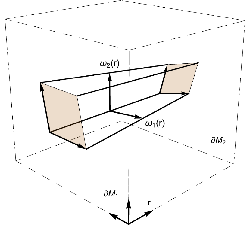
(a)

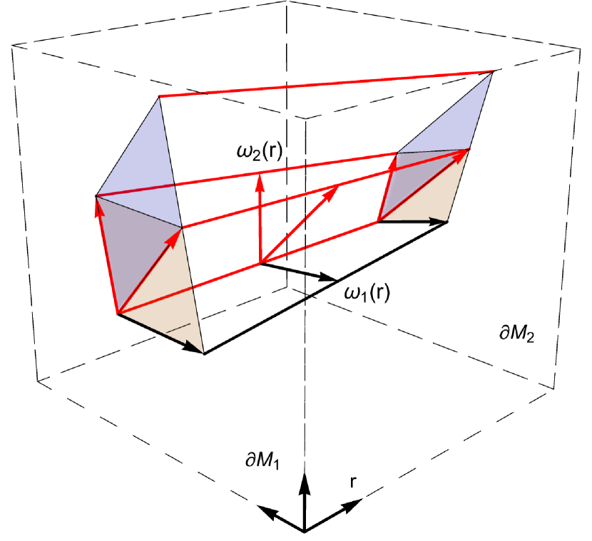
(b)

Figure 1: (a) The two boundaries of $M=T^{2}\times I$ have complex structures induced by choices of lattice bases $\omega_{1,2}(r=0)$ and $\omega_{1,2}(r=1)$ ($r$ is the coordinate on the ‘radial’ direction $I$). (b) A simultaneous modular transformation on the two boundaries is induced by the same change of basis on the two lattices and can be smoothly transported as a large diffeomorphism through the bulk (the transformed bases are colored in red).

a modular transformation on one boundary torus stems from a different choice of basis for the lattice defining it, and this new basis is transported smoothly through the bulk to induce the same change of basis in the second boundary. Therefore the Chern-Simons path-integral $\tilde{Z}_{T^{2}\times I}(\tau_{1},\bar{\tau}_{2})={\rm tr}q_{1}^{L_{0}^{(1)}}\bar{q}_{2}^{L_{0}^{(2)}}$ should be invariant under simultaneous modular transformations

$$\tilde{Z}_{T^{2}\times I}(\gamma\tau_{1},\gamma\bar{\tau}_{2})=\tilde{Z}_{T^{2}\times I}(\tau_{1},\bar{\tau}_{2}).$$ (28)

In this path integral, the two boundaries are oppositely oriented as induced from the bulk. To obtain the partition function for boundary tori with the same orientation, we replace $\tau_{2}\rightarrow-\bar{\tau}_{2}$, leading to

$$Z_{T^{2}\times I}(\tau_{1},\tau_{2})=\tilde{Z}_{T^{2}\times I}(\tau_{1},-\tau_{2}).$$ (29)

It is straightforward to check that the property (28) translates into (26).

The property (26) implies that we can expand the seed amplitude in terms of ${\cal M}$ unknown ‘wormhole coefficients’ $c_{I}$ as follows:

$$Z_{T^{2}\times I}(\tau_{1},\tau_{2})=\sum_{I}c_{I}\chi(\tau_{1})^{T}M_{I}\chi(\tau_{2}).$$ (30)

The equality of the expressions (13) and (15) can once again be expressed as a matrix identity, which can be reduced to

$$\rho_{I}\delta_{IJ}-\rho_{I}\rho_{J}=\sum_{M,N,K,L}\bar{c}_{M}c_{N}(D^{-1})_{IK}(D^{-1})_{JL}D_{MKNL},$$ (31)

where we defined

$$D_{IJKL}={\rm tr}M_{I}M_{J}M_{K}M_{L}.$$ (32)

To derive (31) we have used our assumption (see below (6)) that the $M_{I}$ are real and symmetric matrices.

We should note that (31) is in general an overdetermined system for the ${\cal M}$ complex coefficients $c_{I}$, and it is therefore to be expected that the existence of solutions will also impose constraints on the $\rho_{I}$ and therefore the 1-boundary seed amplitude $Z^{(1)}_{\rm seed}$.

2.5 Wormhole amplitude from canonical quantization

Naively one might expect that the 2-boundary seed amplitude $Z^{(2)}_{\rm seed}$ should be given by the pure Chern-Simons path integral on the $T^{2}\times I$ wormhole geometry. This path integral is the RCFT equivalent of the wormhole partition function computed by Cotler and Jensen for pure gravity and noncompact $U(1)$ Chern-Simons theories Cotler:2020ugk ; Cotler:2020hgz . However, as we shall see, this Chern-Simons path integral, which we will denote as $Z_{T^{2}\times I}^{\rm CS}(\tau_{1},\tau_{2})$, gives only part of the required answer and needs to be supplemented with additional ‘exotic’ wormhole contributions which it will be our task to identify.

Let us first recall the result for the pure Chern-Simons path integral $Z_{T^{2}\times I}^{\rm CS}(\tau_{1},\tau_{2})$ from the standard Chern-Simons/RCFT correspondence. Viewing $T^{2}\times I$ as an annulus $S^{1}\times I$ times a circle representing Euclidean time, we can obtain $Z_{T^{2}\times I}^{\rm CS}(\tau_{1},\tau_{2})$ from the canonical quantization of the theory on the annulus. In this case there are chiral algebras ${\cal A}$ and $\overline{\cal A}$ associated to the two boundary circles of the annulus, and Elitzur:1989nr obtained the following result for the Hilbert space:

$${\cal H}_{S^{1}\times I}=\sum_{i=0}^{{\cal N}-1}{\cal R}_{i}\otimes\overline{{\cal R}_{i}},$$ (33)

where we recall that the ${\cal R}_{i}$ are the irreducible representations of the chiral algebra. Correspondingly, the path intregral is given by (allowing for an undetermined normalization factor $n$)

$$Z_{T^{2}\times I}^{\rm CS}(\tau_{1},\tau_{2})=n\sum_{i=0}^{{\cal N}-1}\chi_{i}(\tau_{1})\chi_{i}(\tau_{2}).$$ (34)

Here, we have followed the steps below (28) to account for boundaries with the same orientation. As a consistency check, we see that this is indeed of the general form (30): it is the particular case where only the diagonal modular invariant $M_{1}^{ij}=\delta^{ij}$ appears. In other words, if the pure Chern-Simons partition function were the full answer, the coefficients $c_{I}$ would be of the form

$$c_{I}^{\rm CS}=n\delta_{I}^{1}.$$ (35)

One remark is in order before we continue to discuss a particular class of RCFT ensembles. For simplicity, we have in this section considered CFT partition functions and characters which only keep track of the Virasoro conformal weights $L_{0}$ and $\bar{L}_{0}$. However, when the chiral algebra is extended, it can be desirable to work with refined partition functions and characters which keep track of further quantum numbers (commuting with $L_{0},\bar{L}_{0}$) and depend on additional chemical potentials. The formulas in this section readily generalize to this setting, provided we assign the proper modular transformation law to the chemical potentials, as we will illustrate in the examples below.

3 Rational boson ensembles and their bulk duals

In what follows we will make the general considerations of the previous Section explicit in a simple class of ensemble holographic theories. In these, the exotic gravity theory is based on a compact $U(1)_{k}\times U(1)_{-k}$ Chern-Simons theory with action

$$S[A,\tilde{A}]=-{k\over 2\pi}\int_{\cal M}(A\wedge dA-\tilde{A}\wedge d\tilde{A}),$$ (36)

where the level $k$ should be an integer in order for the path integral to be well-defined. As shown in Raeymaekers:2021ypf , a large subset of these remains under analytic control even when the size of the ensemble goes to infinity. This will allow us to find explicit expressions for the ensemble weights (20) and to investigate the 2-boundary consistency conditions (31).

3.1 Chiral algebra and representations

The chiral algebra of the models of interest, which we denote as ${\cal A}_{k}$, arises in free boson CFTs at rational values of the radius squared. Indeed, let us consider a compact free boson at radius $R^{2}=p/q$ with $p$ and $q$ relatively prime and positive integers. Setting $k=pq$ this theory has chiral currents

$$J=\partial X(z),\qquad W_{\pm}=:e^{\pm 2i\sqrt{k}X(z)}:$$ (37)

with conformal weights 1 and $k$ respectively. These generate the chiral algebra ${\cal A}_{k}$.

This algebra has $2k$ inequivalent irreducible representations ${\cal R}_{j},j=0,\ldots,2k-1$ Moore:1988ss (for a review, see DiFrancesco:1997nk ). To fully characterize these, we should not only keep track of their weights under the Virasoro generator $L_{0}$ but also under the $u(1)$ generator $J_{0}$. That is, we will work with refined characters defined as

$$\chi_{j}(\tau,z) := {\rm tr}q^{L_{0}}\zeta^{J_{0}}$$ (38)

$$= {1\over\eta(\tau)}\sum_{n\in\mathbb{Z}}q^{(2nk+j)^{2}\over 4k}\zeta^{2nk+j\over 2}$$ (39)

where $q=e^{2\pi i\tau},\zeta=e^{-2\pi iz}$, and $\eta=q^{1\over 24}\prod_{m=1}^{\infty}(1-q^{m})$ is Dedekind’s eta function. The characters satisfy

$$\chi_{2k+j}=\chi_{j}$$ (40)

so we can take $j$ in the range $j=0,\ldots,2k-1$. Charge conjugation sends $j\rightarrow-j$:

$$\chi_{j*}(\tau,z)=\chi_{-j}(\tau,z).$$ (41)

We note that the representations ${\cal R}_{0}$ and ${\cal R}_{k}$ are self-conjugate, while the remaining ${\cal R}_{j}$ with $j\notin k\mathbb{Z}$ are not, since $\chi_{j*}(\tau,z)\neq\chi_{j}(\tau,z)$. However, the specialized characters evaluated at $z=0$ cannot distinguish conjugate representations:

$$\chi_{j*}(\tau,0)=\chi_{j}(\tau,0).$$ (42)

Therefore, in order to keep track of the full ${\cal A}_{k}$ representation content we need to work with refined characters rather than specialized ones.

Under modular transformations $\gamma=\tiny{\left(\begin{array}[]{cc}a&b\\ c&d\end{array}\right)}\in SL(2,\mathbb{Z})$, the characters transform as

$$\chi\left({a\tau+b\over c\tau+d},{z\over c\tau+d}\right)=e^{\frac{i\pi k}{2}\frac{cz^{2}}{c\tau+d}}U_{\gamma}\cdot\chi(\tau,z).$$ (43)

Here, the $U_{\gamma}$ furnish a $2k$-dimensional unitary representation of $SL(2,\mathbb{Z})$. In particular, the modular $S$ and $T$ transformations are represented as

$$T: \chi_{j}(\tau+1,z)= e^{2i\pi\left({j^{2}\over 4k}-{1\over 24}\right)}\chi_{j}(\tau,z)\equiv({\cal T}\chi)_{j},$$ (44)

$$S: \chi_{j}\left(-{1\over\tau},{z\over\tau}\right)= e^{\frac{i\pi kz^{2}}{2\tau}}{1\over\sqrt{2k}}\sum_{j^{\prime}=0}^{2k-1}e^{-2i\pi{jj^{\prime}\over 2k}}\chi_{j^{\prime},k}(\tau,z)\equiv({\cal S}\chi)_{j}.$$ (45)

One checks that the following group relations hold:

$$({\cal S}{\cal T})^{3}={\cal S}^{2}={\cal C},\qquad{\cal C}^{2}=1.$$ (46)

Since the charge conjugation matrix ${\cal C}$ is not the identity, the matrices $U_{\gamma}$ furnish a representation of $SL(2,\mathbb{Z})$ rather than $PSL(2,\mathbb{Z})$.

Due to the $z$-dependent prefactor in (45), the refined characters do not transform in a matrix representation of $SL(2,\mathbb{Z})$ under modular transformations. This can be remedied by multiplying the characters by an extra factor whose transformation offsets the anomalous part. Indeed, one checks that

$$\tilde{\chi}_{j}(\tau,z)=e^{\pi k{z^{2}\over 4\tau_{2}}}\chi_{j}(\tau,z)$$ (47)

transforms in the unitary matrix representation of $SL(2,\mathbb{Z})$ furnished by the matrices $U_{\gamma}$.

We should also note that the rescaled characters $\tilde{\chi}(\tau,z)$ are the ones that naturally appear in expressions obtained from a covariant path integral formulation Kraus:2006nb . In the 2D free boson theory, the chemical potential $z$ is introduced in the Lagrangian by adding a term of the form ${\cal A}_{\bar{w}}\partial_{w}X+{\cal A}_{w}\partial_{\bar{w}}X$, where ${\cal A}_{\bar{w}}\propto z$ . In converting to Hamiltonian form one gets a cross term proportional to ${\cal A}_{w}{\cal A}_{\bar{w}}$ which is precisely the prefactor in (48). The argument extends to 3D Chern-Simons path integrals, e.g. the path integral on the solid torus with appropriate boundary conditions is proportional to $|\tilde{\chi}_{0}(\tau,z)|^{2}$ Datta:2021ftn .

3.2 Modular invariants

Let us now discuss the modular invariant combinations of ${\cal A}_{k}\times\overline{{\cal A}}_{k}$ characters. From the construction above we note that, for each divisor $\delta$ of $k$ (which we will write as $\delta|k$ in what follows), the compact boson at radius $R^{2}=k/\delta^{2}$ yields a realization of the algebra ${\cal A}_{k}\times\overline{{\cal A}}_{k}$. The refined and rescaled partition function

$$Z_{R}[\tau,z]=e^{\pi k{z^{2}+\bar{z}^{2}\over 4\tau_{2}}}{\rm tr}_{{\cal H}_{R}}q^{L_{0}}\bar{q}^{\tilde{L}_{0}}\zeta^{J_{0}}\bar{\zeta}^{\tilde{J}_{0}}$$ (48)

therefore furnishes a modular invariant. Furthermore, a full analysis of the commutant of the ${\cal S}$- and ${\cal T}$-matrices Cappelli:1986hf ; Cappelli:1987xt shows that the modular invariants obtained in this way form a complete basis. It follows that in these theories, the number of independent modular invariants is ${\cal M}=d(k)$, the number of distinct divisors of $k$.

It will be convenient to introduce a specific labelling of the modular invariant partition functions. For this we first label the divisors of $k$ with an index $I$ running from 1 to $d(k)$ in increasing order

$$1=\delta_{1}<\delta_{2}\ldots<\delta_{d(k)}.$$ (49)

We will use the same label to indicate the modular invariant partition function associated to $\delta_{I}$, i.e.

$$Z_{I}[\tau,z]\equiv Z_{R={\sqrt{k}\over\delta_{I}}}[\tau,z].$$ (50)

As before we associate to $Z_{I}$ a modular invariant $2k\times 2k$ matrix $M_{I}$ through decomposition in (rescaled) characters

$$Z_{I}[\tau,z]=\tilde{\chi}(\tau,z)^{\dagger}M_{I}\tilde{\chi}(\tau,z).$$ (51)

Let us now give an explicit expression for these matrices $M_{I}$.

It will be useful to introduce the symbol $\alpha_{I}$ to denote the greatest common denominator of $\delta_{I}$ and $k/\delta_{I}$:

$$\alpha_{I}:=\gcd\left(\delta_{I},{k\over\delta_{I}}\right).$$ (52)

Note that $\alpha_{I}$ is a quadratic divisor of $k$, $\alpha_{I}^{2}|k$. The definition (52) and Bezout’s lemma imply that there exist integers $r_{I},s_{I}$ such that

$$r_{I}{\delta_{I}\over\alpha_{I}}-s_{I}{k\over\alpha_{I}\delta_{I}}=1.$$ (53)

From these we define the quantity $\omega_{I}$ as follows

$$\omega_{I}=\left[r_{I}{\delta_{I}\over\alpha_{I}}+s_{I}{k\over\alpha_{I}\delta_{I}}\right]_{2k\over\alpha_{I}^{2}},$$ (54)

where we introduced the notation $[x]_{n}:=x\mod n$. We note that $\omega_{I}$ is defined modulo $2k/\alpha_{I}^{2}$, and it is straightforward to check that a different choice of $r_{I}$ and $s_{I}$ leads to the same $\omega_{I}$. Furthermore, $\omega_{I}$ are roots of unity modulo $4k/\alpha_{I}^{2}$,

$$\omega_{I}^{2}:=1\mod{{4k\over\alpha_{I}^{2}}}.$$ (55)

With these definitions, the components of the modular invariant matrices $M_{I}$ in (51) are Raeymaekers:2021ypf

$$M_{I}^{ij}=\left\{\begin{array}[]{ll}{1\over\alpha_{I}}\delta_{[i-\omega_{I}j]_{2k\over\alpha_{I}}}&{\ \rm if\ }\alpha_{I}|i{\rm\ and\ }\alpha_{I}|j\\ 0&{\ \rm otherwise}\end{array}\right.,\qquad 0\leq i,j<2k.$$ (56)

Here, the quantity $\delta_{[x]_{n}}$ is defined to be one if $x\equiv 0\ ({\rm mod\ }n)$ and zero otherwise. We note that all these modular invariants are physical in the sense of Section 2: the coefficients in the character decomposition are positive integers and the vacuum representation occurs precisely once, $M_{I}^{00}=1,\forall I$. We note that the uniqueness of the vacuum fixes the normalization of the modular matrices, preventing us from multiplying them by some positive natural number.

We close this subsection with a remark on T-duality. Since, in our labelling (49), $\omega_{1}=1$ and $\omega_{d(k)}=-1$, the corresponding modular invariant matrices are

$$M_{1}=1,\qquad M_{d(k)}={\cal C}.$$ (57)

These cases correspond to the diagonal and to the charge conjugation modular invariant respectively. More generally, the root of unity associated to $k/\delta_{I}$ is $-\omega_{I}$ and their modular matrices are related as

$$M_{\delta_{I}}={\cal C}M_{k\over\delta_{I}}.$$ (58)

Therefore, due to (42), at vanishing chemical potential their partition functions are the same,

$$Z_{\sqrt{k}\over\delta_{I}}[\tau,0]=Z_{\delta_{I}\over\sqrt{k}}[\tau,0]$$ (59)

which expresses the standard T-duality invariance of the compact boson partition function.

3.3 Monoidal multiplicative structure

Before proceeding, let us comment on the further structure on the space of the modular invariant matrices. From the component form (56) one can deduce that multiplying two modular invariant matrices gives again a modular invariant matrix. Concretely (see Raeymaekers:2021ypf for details) one finds

$$M(\omega_{I})M(\omega_{J})=\gcd(\alpha_{I},\alpha_{J})M\left(\omega_{I}\bullet\omega_{J}\right)$$ (60)

where $\bullet$ stands for the following multiplication rule

$$\omega_{I}\bullet\omega_{J}=[\omega_{I}\omega_{J}]_{2k\over{\rm lcm}(\alpha_{I},\alpha_{J})^{2}}.$$ (61)

The prefactor on the RHS could, at the cost of working with non-physical modular matrices, be absorbed in a rescaling of the $M_{I}$ by a factor $\alpha_{I}^{-1}$; one then sees that the rescaled matrices form a monoid under multiplication. This is consistent with the fact that modular invariants are in one-to-one correspondence with topological surface operators in the Chern-Simons theory. As we shall show in detail in Section 5, the multiplication rule (60) agrees with the fusion rule for these defects, which define a monoidal two-category.

This additional structure becomes even more restrictive in the case where $k$ is square-free, meaning that it has no non-trivial square divisors $\beta^{2}|k,\beta>1$, so that the numbers $\alpha_{I}$ defined above are all equal to one. In this case the monoidal structure simplifies to an actual group structure. More precisely, the modular matrices form a representation of the multiplicative group $G_{k}$ of roots of unity modulo $2k$,

$$G_{k}=\{[\omega]_{2k};\omega^{2}\equiv 1\ ({\rm mod\ }2k)\}.$$ (62)

To show this, we first note that, for the modular invariant associated to the divisor $\delta_{I}$, the quantity $\omega_{I}$ defined in (54) with $\alpha_{I}=1$ is an element of $G_{k}$ due to (55). Conversely, to every element $\omega\in G_{k}$ one can associate the divisor

$$\delta(\omega):=\gcd\left(\frac{\omega+1}{2},k\right).$$ (63)

Notice that, by definition, $\omega$ is its own multiplicative inverse modulo $2k$ hence it must be coprime with $2k$. So every $\omega\in G_{k}$ is in particular odd and the quantity $\frac{\omega+1}{2}$ is an integer. Moreover $\delta(\omega)$ is well defined even if $\omega$ is defined modulo $2k$, because of the property $\gcd(a+mk,k)=\gcd(a,k)$. One can check that the definitions (54) and (63) are each others inverse, providing a one-to-one correspondence between the set of divisors of $k$ and the elements of $G_{k}$. In this special case, from the component expression (56) we see that the modular invariant matrices $M_{I}$ furnish the $2k$-dimensional representation corresponding simply to the multiplication by $\omega_{I}$ in $\mathbb{Z}_{2k}$.

For generic $k$, the multiplication rules (60) show that the modular matrices form a representation of a commutative monoid with unit element. It can be seen to possess the following structure

$$G_{k}=\bigcup_{\alpha\in\mathrm{SqDiv}(k)}G^{\alpha}_{k},\qquad G_{k}^{\alpha}:=\{[\omega]_{2k/\alpha^{2}};\omega^{2}\equiv 1\ ({\rm mod\ }4k/\alpha^{2})\}.$$ (64)

Here, corresponding to each square-divisor $\alpha$ there is a maximal subgroup $G^{\alpha}_{k}$ which is one-to-one with the subset of divisors of $k$ satisfying $\gcd(\delta,k/\delta)=\alpha$. This can be shown similarly to above, generalizing (63) to

$$\omega\in G^{\alpha}_{k}:\qquad\delta(\omega):=\alpha\gcd\left(\frac{\omega+1}{2},\frac{k}{\alpha^{2}}\right)$$ (65)

which inverts (54) in the general case. This provides a one-to-one correspondence between the set of divisors of $k$ and $G_{k}$ in full generality.

4 Analysis of the two-boundary constraints

Having set the stage, we will in the rest of this work explore the solutions to the equations (20) determining the ensemble weights and the two-boundary consistency conditions (31).

4.1 Examples for small $k$

It will prove instructive to first consider the problem for a few simple cases at low values of $k$ as we shall do presently; in the next subsection we will then find the general solution for square-free $k$.

4.1.1 $k=1$

In this simplest example, there are two irreducible representations $({\cal N}=2$) and only one possible modular invariant $({\cal M}=1)$, the diagonal one. Hence there is no ensemble to average over and (31) indeed tells us that the wormhole coefficient $c_{1}$ should vanish.

4.1.2 $k=2$

In this example there are four representations $({\cal N}=4$) and two modular invariants $({\cal M}=2$). In our labelling convention we have

$$\delta_{I}=(1,2),\qquad\alpha_{I}=(1,1),\qquad\omega_{I}=\left([1]_{4},[-1]_{4}\right),$$ (66)

and the modular invariant matrices are the identity and the charge conjugation matrix ${\cal C}$

$$M_{1}=1,\qquad M_{2}={\cal C}={\small\left(\begin{array}[]{cccc}1&0&0&0\\ 0&0&0&1\\ 0&0&1&0\\ 0&1&0&0\end{array}\right)}.$$ (67)

Since ${\cal C}^{2}=1$ the group they form under multiplication is isomorphic to $\mathbb{Z}_{2}$. The matrix $D_{IJ}$ defined in (22) is equal to

$$D_{IJ}={\small\left(\begin{array}[]{cc}4&2\\ 2&4\end{array}\right)}.$$ (68)

Starting from a general seed vector

$$V^{\rm seed}_{I}=(v_{1},v_{2})$$ (69)

we find from (20) the ensemble weights

$$\rho_{I}=\left({2v_{1}-v_{2}\over v_{1}+v_{2}},{2v_{2}-v_{1}\over v_{1}+v_{2}}\right).$$ (70)

In order for the weights to take values between zero and one the seed vector needs to satisfy

$${1\over 2}\leq{v_{1}\over v_{2}}\leq 2.$$ (71)

The special case of the vacuum seed vector $V^{\rm seed}=(1,1)$ (cfr. (24)) leads to equal ensemble weights, $\rho_{I}={1\over 2}(1,1)$.

Next we turn to the equations (31) for the wormhole coefficients $c_{I}$. In this example the system is solvable for general ensemble weights, and the solution is only determined up to an overall phase $\theta_{2}$:

$$c_{I}=\sqrt{\rho_{1}\rho_{2}}e^{i\theta_{2}}(1,-1).$$ (72)

This example generalizes to the situation where $k$ is a prime number in a straightforward way.

The examples with only 1 or 2 modular invariants considered so far are special; for a greater number of modular invariants (31) also places constraints on the ensemble weights $\rho_{I}$, as the two following examples show.

4.1.3 $k=6$

In this case, ${\cal N}=12,{\cal M}=4$ and we have

$$\delta_{I}=(1,2,3,6),\qquad\alpha_{I}=1,\qquad\omega_{I}=\left([1]_{12},[7]_{12},[5]_{12},[11]_{12}\right).$$ (73)

Working out the modular invariant matrices from (56) one finds that they form a group isomorphic to $(\mathbb{Z}_{2})^{2}$, more precisely

$$M_{1}\simeq(1,1),\qquad M_{2}\simeq(-1,1),\qquad M_{3}\simeq(1,-1)\qquad M_{4}\simeq(-1,-1).$$ (74)

The matrix $D_{IJ}$ is found to be

$$D_{IJ}={\small\left(\begin{array}[]{cccc}12&6&4&2\\ 6&12&2&4\\ 4&2&12&6\\ 2&4&6&12\\ \end{array}\right)},$$ (75)

and a general 1-boundary seed vector $V^{\rm seed}_{I}=(v_{1},v_{2},v_{3},v_{4})$ leads to the ensemble weights

$$\rho_{I}=\left(\frac{6{v_{1}}-3{v_{2}}-2{v_{3}}+{v_{4}}}{2({v_{1}}+{v_{2}}+{v_{3}}+{v_{4}})},\frac{-3{v_{1}}+6{v_{2}}+{v_{3}}-2{v_{4}}}{2({v_{1}}+{v_{2}}+{v_{3}}+{v_{4}})},\frac{-2{v_{1}}+{v_{2}}+6{v_{3}}-3{v_{4}}}{2({v_{1}}+{v_{2}}+{v_{3}}+{v_{4}})},\frac{{v_{1}}-2{v_{2}}-3{v_{3}}+6{v_{4}}}{2({v_{1}}+{v_{2}}+{v_{3}}+{v_{4}})}\right).$$ (76)

Positivity of the $\rho_{I}$ again restricts the allowed ranges of the $v_{I}$.

Next we turn to the 2-boundary consistency constraints (31). We first convert to a basis in which the RHS of (31) is diagonal. In order for solutions to exist, the LHS must also be diagonal in this basis, which places restrictions on the allowed seed vector $V^{\rm seed}$. One finds that these lead to two classes of admissible seed vectors. Either it is (up to an overall rescaling) of the form $v_{I}={\rm tr}M_{I}M_{J}$, for some $J$. In this case, the 1-boundary seed amplitude is already modular invariant and given by $M_{J}$. This picks out a single CFT theory, $\rho_{I}=\delta_{IJ}$, rather than an ensemble, and the wormhole coefficients $c_{I}$ consequently vanish.

The second consistent possibility, and the only one leading to an ensemble of theories, is that seed vector is (up to rescaling) $v_{I}=(1,1,1,1)$. This arises most naturally from the vacuum seed amplitude (18), but it could also come from starting with the charge-$k$ excited state $Z^{(1)}_{\rm seed}=\tilde{n}|\tilde{\chi}_{k}|^{2}$. We see from (76) that the seed vector $v_{I}=(1,1,1,1)$ leads to a maximal entropy ensemble with

$$\rho_{I}=\frac{1}{4}(1,1,1,1).$$ (77)

The solution for the corresponding wormhole coefficients is determined up to 3 phases, which for later comparison we label as $\theta_{2,3,4}$; one finds

$$c_{I} = \frac{1}{4}\left(e^{i\theta_{2}}+\sqrt{2}e^{i\theta_{3}}+\sqrt{3}e^{i\theta_{4}},-e^{i\theta_{2}}-\sqrt{2}e^{i\theta_{3}}+\sqrt{3}e^{i\theta_{4}},\right.$$ (78)

$$\left.-e^{i\theta_{2}}+\sqrt{2}e^{i\theta_{3}}-\sqrt{3}e^{i\theta_{4}},e^{i\theta_{2}}-\sqrt{2}e^{i\theta_{3}}-\sqrt{3}e^{i\theta_{4}}\right).$$

4.1.4 $k=9$

In this example, $k$ is not square-free. We have ${\cal N}=18,{\cal M}=3$ and

$$\delta_{I}=(1,3,9),\qquad\alpha_{I}=(1,3,1),\qquad\omega_{I}=(1,1,17).$$ (79)

The modular matrices form a monoid under multiplication, with $M_{1}$ playing the role of an identity element and

$$M_{2}\cdot M_{2}=3M_{2},\qquad M_{2}\cdot M_{3}=M_{2},\qquad M_{3}\cdot M_{3}=M_{1}.$$ (80)

In other words, $M_{2}$ does not possess an inverse. Note that $M_{1},M_{3}$ form a $\mathbb{Z}_{2}$ subgroup.

Denoting again $V^{\rm seed}=(v_{1},v_{2},v_{3})$, the general ensemble weights are

$$\rho_{I}=\left(\frac{3(3{v_{1}}-{v_{2}})}{2(3{v_{1}}+2{v_{2}}+3{v_{3}})},\frac{-3{v_{1}}+10{v_{2}}-3{v_{3}}}{2(3{v_{1}}+2{v_{2}}+3{v_{3}})},-\frac{3({v_{2}}-3{v_{3}})}{2(3{v_{1}}+2{v_{2}}+3{v_{3}})}\right).$$ (81)

We note that, in contrast with the previous examples, starting from the vacuum seed vector $v_{I}=(1,1,1)$ does not lead to a uniform distribution but to $\rho_{I}=(3/8,1/4,3/8)$.

An analysis of the 2-boundary consistency conditions (31) for the wormhole coefficients shows that only two types of solutions are possible. As in the previous example, a trivial class of solutions occurs when we start from a modular invariant 1-boundary seed amplitude, in which case there is no ensemble and the wormhole amplitude vanishes, $c_{I}=0$. The second possibility occurs when the seed vector is such that the non-invertible invariant $M_{2}$ doesn’t appear in the ensemble, i.e. $\rho_{2}=0$. From (81) this happens for

$$v_{2}={3\over 10}(v_{1}+v_{3}).$$ (82)

The analysis proceeds as in the $k=2$ case, as we are left with an ensemble containing 2 modular invariants forming a $\mathbb{Z}_{2}$ group. The solutions in this class have

$$\rho_{I} =\left(\frac{9{v_{1}}-{v_{3}}}{8({v_{1}}+{v_{3}})},0,\frac{9{v_{3}}-{v_{1}}}{8({v_{1}}+{v_{3}})}\right),$$ (83)

$$c_{I} =\sqrt{8\rho_{1}\rho_{3}}e^{i\theta}(1,0,-1).$$

One can check that these exhaust all consistent possibilities. We note in particular that starting from the vacuum seed $V^{\rm seed}\propto(1,1,1)$ is in this case ruled out.

4.2 General solution for square-free $k$

The first three examples above belong to the class where $k$ is square-free. We will now derive an explicit formula the ensemble weights (20) and analyze the consistent solutions to the 2-boundary constraints (31) within this class of rational boson ensembles.

We recall that the modular invariant matrices form a group under multiplication, which is isomorphic to the group $G_{k}$ of roots of unity modulo $2k$,

$$G_{k}=\{[\omega]_{2k};\omega^{2}\equiv 1\ ({\rm mod\ }2k)\}.$$ (84)

Since $k$ is square-free, its prime decomposition is of the form $k=p_{1}p_{2}\ldots p_{\Omega(k)}$ with all $p_{\rho}$ distinct, and the number of elements of $G_{k}$ is $d(k)=2^{\Omega(k)}$. This is also the number of independent modular invariants which we denoted by ${\cal M}$:

$${\cal M}=|G_{k}|=2^{\Omega(k)}.$$ (85)

The group $G_{k}$ is commutative and, apart from the unit element $\omega_{1}$, all group elements have order two. A standard result Omami:2009 shows that $G_{k}$ is in fact isomorphic to $(\mathbb{Z}_{2})^{\Omega(k)}$. The group $(\mathbb{Z}_{2})^{\Omega(k)}$ is generated by $\Omega(k)$ ‘odd elements’ which, under the isomorphism correspond to

$$\omega(p_{\rho}),\qquad\rho=1,\ldots,\Omega(k).$$ (86)

For example, when $k=6$ (see (74)) these odd elements are given by $\omega(2)=[7]_{12}\simeq(-1,1)$ and $\omega(3)=[5]_{12}\simeq(1,-1)$.

4.2.1 Some representation theory

In what follows we will need some representation theory of $G_{k}$. Let us first discuss its irreducible representations (irreps). Since $G_{k}$ is a commutative group, all the irreps are one-dimensional, and their number equals ${\cal M}=2^{\Omega(k)}$, the order of the group. Since each group element squares to one, the irreps can only take the values 1 or -1. An irrep is fully specified by giving its value on each of the generating elements $\omega(p_{\rho})$, leading indeed to $2^{\Omega(k)}$ sign choices. We will label the irreps as $\sigma^{\alpha},\alpha=1,\ldots,{\cal M}$. For fixed $\alpha$, we can view $\sigma^{\alpha}$ as a ${\cal M}$-dimensional vector with components

$$(\sigma^{\alpha})_{I}\equiv\sigma^{\alpha}(\omega_{I})$$ (87)

taking the values 1 or -1. We adopt the convention that $\sigma^{1}$ is the trivial representation, i.e.

$$(\sigma^{1})_{I}=1,\qquad\forall I.$$ (88)

The orthogonality relations between irreducible characters can be expressed as follows:

$$\sum_{I}(\sigma^{\alpha})_{I}(\sigma^{\beta})_{I}={\cal M}\delta^{\alpha\beta},\qquad\sum_{\alpha}(\sigma^{\alpha})_{I}(\sigma^{\alpha})_{J}={\cal M}\delta_{IJ}.$$ (89)

Next we turn to the regular representation which we denote as $R$, and whose matrices we write as $R_{I}\equiv R(\omega_{I})$. $R$ is the ${\cal M}$-dimensional representation corresponding to the action of the group on itself

$$\omega_{I}\omega_{J}=(R_{I})_{J}^{\ \,K}\omega_{K}.$$ (90)

The representation matrices $R_{I}$ are symmetric, commuting, permutation matrices which square to one. A standard property for abelian groups is that each irrep appears precisely once in the decomposition of $R$,

$$R=\oplus_{\alpha=1}^{{\cal M}}\sigma^{\alpha}.$$ (91)

The basis in which the $R$ matrices are block-diagonal according to the above decomposition is provided by the vectors $\sigma^{\alpha}$. Indeed, one shows that

$$R_{I}\cdot\sigma^{\alpha}=\sigma^{\alpha}(\omega_{I})\sigma^{\alpha},$$ (92)

which follows from

$$\sigma^{\alpha}(\omega_{I})\sigma^{\alpha}(\omega_{J}) =\sigma^{\alpha}\left(\sum_{K}(R_{I})_{J}^{\ K}\omega_{K}\right)$$ (93)

$$=\sum_{K}(R_{I})_{J}^{\ K}\sigma^{\alpha}(\omega_{K}).$$

A useful identity following from (92) is that the regular representation matrices can be expressed as

$$(R_{I})_{J}^{\ \,K}={1\over{\cal M}}\sum_{\alpha}\sigma^{\alpha}(\omega_{I}\omega_{J}\omega_{K}).$$ (94)

A last representation which plays a role in our problem corresponds to the natural action of $\omega\in G_{k}$ on $\mathbb{Z}_{2k}$ by multiplication, $[i]_{2k}\rightarrow[\omega i]_{2k}$. We denote this representation by $M$ and write $M(\omega_{I})\equiv M_{I}$. We see from (56) that the $M_{I}$ are precisely the modular invariant matrices introduced before. We denote by $m^{\alpha}$ the multiplicity of the irrep $\sigma^{\alpha}$ in the decomposition of $M$:

$$M=\oplus_{\alpha=1}^{{\cal M}}m^{\alpha}\sigma^{\alpha}.$$ (95)

Let us say a bit more about these multiplicities. It is straightforward to see that the trivial representation appears at least twice, i.e.

$$m^{1}\geq 2.$$ (96)

Indeed, since the congruence $[0]_{2k}$ is invariant under multiplication by $\omega_{I}$, it defines an invariant subspace. A second invariant subspace is the congruence $[k]_{2k}$, which is mapped to itself under multiplication by $\omega_{I}$ since, as we established below eq. (63), the $\omega_{I}$ are odd. In other words, we have

$$(M_{I})^{00}=(M_{I})^{kk}=1=(\sigma^{1})_{I},\qquad\forall I.$$ (97)

In CFT terms this means that each modular invariant contains the (vacuum, vacuum) and the $(k,k)$ representation precisely once. As for the other multiplicities in (101), we will see below (105) that they are all nonvanishing:

$$m^{\alpha}\geq 1,\qquad\forall\alpha.$$ (98)

Note that the properties (96) and (98) imply that the representation $M$ is always bigger than the regular representation $R$. The decomposition (56) implies a similar expansion for the characters, ${\rm tr}M_{I}=\sum_{\alpha}m^{\alpha}(\sigma^{\alpha})_{I}$, which can be inverted to give an formula for the multiplicities $m^{\alpha}$:

$$m^{\alpha}={1\over{\cal M}}\sum_{I}(\sigma^{\alpha})_{I}{\rm tr}M_{I}.$$ (99)

4.2.2 General formula for the ensemble weights

Using these properties, we can rewrite the expression (20) for the ensemble weights $\rho^{I}$ in a theory with generic seed amplitude purely in terms of representation-theoretic quantities. Recall that (20) takes the form

$$\rho_{I}=n\sum_{J}(D^{-1})_{IJ}(V^{\rm seed})_{J},$$ (100)

where $n$ is determined by the normalization condition that $\sum_{I}\rho_{I}=1$. First we observe that the matrix $D_{IJ}={\rm tr}M_{I}M_{J}$ becomes diagonal in the $\{\sigma^{\alpha}\}$ basis:

$$D_{IJ} =\sum_{\alpha}m^{\alpha}(\sigma^{\alpha})_{I}(\sigma^{\alpha})_{J},$$ (101)

$$D_{\alpha\beta} =\sum_{IJ}(\sigma^{\alpha})_{I}D_{IJ}(\sigma^{\beta})_{J}=\mathcal{M}^{2}m^{\alpha}\delta_{\alpha\beta},$$

where we used the orthogonality relations (89). Since $D_{IJ}$ can be shown to be invertible, it follows that all the multiplicities $m^{\alpha}$ are nonvanishing, as anticipated in (98) above. Therefore its inverse is

$$(D^{-1})_{IJ} = {1\over{\cal M}^{2}}\sum_{\alpha}(m^{\alpha})^{-1}(\sigma^{\alpha})_{I}(\sigma^{\alpha})_{J}={1\over{\cal M}^{2}}\sum_{\alpha}(m^{\alpha})^{-1}\sigma^{\alpha}(\omega_{I}\omega_{J}).$$ (102)

To proceed it will be useful to also define the components of various vectors appearing in the problem in the $\{\sigma^{\alpha}\}$ basis:

$$v^{\alpha}=\sum_{I}(V^{\rm seed})_{I}(\sigma^{\alpha})_{I},\qquad\rho^{\alpha}=\sum_{I}\rho_{I}(\sigma^{\alpha})_{I},\qquad c^{\alpha}=\sum_{I}c_{I}(\sigma^{\alpha})_{I}.$$ (103)

In order for the seed amplitude to lead to sensible ensemble weights satisfying $\sum_{I}\rho_{I}=1$, it is necessary that $v^{1}\neq 0$, or equivalently, $\sum_{I}v_{I}\neq 0$. The formula (100) can be simply rewritten as

$$\rho^{\alpha}={v^{\alpha}\over v^{1}}{m^{1}\over m^{\alpha}},$$ (104)

and converting back to the Carthesian basis we get

$$\rho_{I}={1\over{\cal M}}\sum_{\alpha}{v^{\alpha}\over v^{1}}{m^{1}\over m^{\alpha}}(\sigma^{\alpha})_{I}.$$ (105)

This is our-sought-after general formula for the ensemble weights. Note that in the special case of the vacuum seed vector, we have $v^{\alpha}\propto\delta^{\alpha}_{1}$ and we reproduce the result of Raeymaekers:2021ypf that the ensemble weights are equal, $\rho_{I}={\cal M}^{-1},\ \forall I$.

4.2.3 Two-boundary consistency conditions

Now let us try to solve the consistency conditions (31) to determine the wormhole coefficients $c_{I}$. Due to being a highly overdetermined system, the existence if solutions will also place constraints on the allowed seed vectors. The equations (31) can be written as

$$\sum_{M,N}\bar{c}_{M}c_{N}(R_{M}R_{N})_{IJ} = \sum_{K}D_{IK}(\rho_{K}\delta_{KJ}-\rho_{K}\rho_{J})$$ (106)

$$= \rho_{J}\left(D_{IJ}-{\cal M}{m^{1}\over v^{1}}(V^{\rm seed})_{I}\right),$$

where in the second line we used (105). Using the identity (94), multiplying both sides with $(\sigma^{\alpha})_{K}$ and summing over $K$, the system (106) can be reduced to

$$\left|c^{\alpha}\right|^{2}={\cal M}m^{\alpha}\rho_{I}\left(1-\rho^{\alpha}(\sigma^{\alpha})_{I}\right),\qquad\forall\alpha,I.$$ (107)

Summing (107) over all $I$ leads to the equation

$$\left|c^{\alpha}\right|^{2}=m^{\alpha}\left(1-(\rho^{\alpha})^{2}\right),$$ (108)

which determines the coefficients $c_{I}$ up to phases:

$$c_{I}={1\over{\cal M}}\sum_{\alpha}\sqrt{m^{\alpha}}\sqrt{1-(\rho^{\alpha})^{2}}e^{i\theta_{\alpha}}(\sigma^{\alpha})_{I}.$$ (109)

We still have to check whether the remaining equations in the system (107) are satisfied. Substituting (108) into (107) yields

$$1-(\rho^{\alpha})^{2}={\cal M}\left(1-(\sigma^{\alpha})_{I}\rho^{\alpha}\right)\rho_{I},\qquad\forall\alpha,I.$$ (110)

This system can be viewed as a set of highly restrictive constraints on the 1-boundary seed coefficients $v^{\alpha}$. Let us now find all the solutions which make physical sense.

Summing (110) over $\alpha$, we obtain

$$\rho_{I}(1-\rho_{I})={1\over{\cal M}}\left(1-\sum_{J}\rho_{J}^{2}\right)\equiv X\qquad\forall I.$$ (111)

We note that the RHS is independent of $I$, so this equation restricts each $\rho_{I}$ to be a root of the same quadratic equation.

The case ${\cal M}=2$ is special, since (111) is automatically satisfied for $\rho_{2}=(1-\rho_{1})$, and so is (110). Therefore for ${\cal M}=2$ the $\rho_{I}$ are unrestricted and the general solution for the wormhole coefficients (109) reduces to

$$c_{I}=\sqrt{m^{2}\rho_{1}\rho_{2}}e^{i\theta_{2}}(1,-1)$$ (112)

Now let us analyze the situation where ${\cal M}>2$. The general solution of (111) is determined by ${\cal M}$ sign choices $s_{I}=\pm 1,I=1,\ldots,{\cal M}$ for the branches of the roots of quadratic equations (111):

$$\rho_{I}={1\over 2}\left(1-s_{I}\sqrt{1-4X}\right).$$ (113)

Summing over $I$ and using (7) we find that at least half of the $s_{I}$ should be equal to 1, since

$$\sum_{I}s_{I}={{\cal M}-2\over\sqrt{1-4X}}>0.$$ (114)

Substituting into (113) gives

$$\rho_{I}={1\over 2}\left(1-{{\cal M}-2\over\sum_{J}s_{J}}s_{I}\right).$$ (115)

For each choice of the $s_{I}$ which sum to a positive number we should in principle check if the full set of equations (110) is obeyed. This would be a daunting task in general, but in practice we can restrict attention to those cases where the $\rho_{I}$ in (115) are positive. This will reduce our work to checking only two cases.

The first case to verify is that where all $s_{I}=1$. This leads to

$$\rho_{I} ={1\over{\cal M}}, \rho^{\alpha} =\delta^{\alpha}_{1}, v^{\alpha} =v^{1}\delta^{\alpha}_{1},$$ (116)

and it is straightforward to check that (110) is obeyed. This case includes our natural starting point of the vacuum seed amplitude, $Z_{\rm seed}^{(1)}\propto|\tilde{\chi}_{0}|^{2}$ but, due to (97) one could just as well take $Z_{\rm seed}^{(1)}\propto|\tilde{\chi}_{k}|^{2}$. The formula (109) gives the expression for the wormhole coefficients

$$c_{I}={1\over{\cal M}}\sum_{\alpha=2}^{\cal M}\sqrt{m^{\alpha}}e^{i\theta_{\alpha}}\sigma^{\alpha}(\omega_{I}).$$ (117)

The next case to check is that where all except one of $s_{I}$ are equal to one, say $s_{J}=-1$ for some $J$. This leads to

$$\rho_{I} =\delta_{IJ}, \rho^{\alpha} =(\sigma^{\alpha})_{J}, v^{\alpha} ={v^{1}m^{\alpha}\over m^{1}}(\sigma^{\alpha})_{J}.$$ (118)

This also trivially satisfies (110). The first relation shows that there is no ensemble and (109) shows that the corresponding wormhole coefficients vanish,

$$c_{I}=0,\qquad\forall I.$$ (119)

This class arises if we start with a seed amplitude which is already modular invariant, $Z_{\rm seed}^{(1)}\propto Z_{J}^{\rm CFT}$ for some $J$.

Next we should consider the case where precisely two of the signs, say $s_{J},s_{K}$ for some $J\neq K$, are equal to minus one. Note that this requires ${\cal M}>4$. Then the expression (115) gives

$$\rho_{I}=-{1\over{\cal M}-4}<0,\qquad{\rm for\ }I\neq J,K.$$ (120)

Similarly, one shows that all remaining choices for the $s_{I}$ would lead to negative ensemble weights and can therefore be discarded.

As a check on our formulas it is useful to compare them to our earlier computations in simple examples. For $k=2$, we have

$$(\sigma^{\alpha})_{I}={\small\left(\begin{array}[]{cc}1&1\\ 1&-1\end{array}\right)},\qquad m^{\alpha}=(3,1).$$ (121)

One checks that our equations (105) for the ensemble weight and (112) for the wormhole coefficients in the case ${\cal M}=2$ match with our earlier results (70) and (72). For $k=6$, one finds

$$(\sigma^{\alpha})_{I}={\small\left(\begin{array}[]{cccc}1&1&1&1\\ 1&-1&-1&1\\ 1&-1&1&-1\\ 1&-1&1&-1\end{array}\right)},\qquad m^{\alpha}=(6,1,2,3).$$ (122)

With these in hand one checks that (105) reproduces the ensemble weights (76), and that the formula (117) for the wormhole coefficients with vacuum seed reproduces (78).

While we defer the general lessons to be learned from this rather technical analysis to the Discussion, we will first focus on one prominent feature: the need to include somewhat exotic wormholes and their relation to topological surface defects.

5 Exotic wormholes from surface defects

Both in the examples and in the general discussion, we have seen that, in sitations which describe an ensemble, the wormhole coefficients $c_{I}$ are typically all nonvanishing (see e.g. (109)). Therefore the two-boundary seed amplitude

$$Z_{\mathrm{seed}}^{(2)}=|Z_{T^{2}\times I}|^{2},\qquad Z_{T^{2}\times I}(\tau_{1},\tau_{2})=\sum_{J}c_{J}\chi(\tau_{1})^{T}M_{J}\chi(\tau_{2})$$ (123)

includes, besides the $J=1$ term which we saw in Section (2.5) comes from the standard pure $U(1)_{k}$ Chern-Simons path integral (34) on the wormhole geometry, also other terms which represent some kind of exotic wormhole contributions. These correspond to 2-boundary amplitudes seed constructed from nondiagonal modular invariants. As we shall presently describe, these have a nice bulk interpretation in terms of path integrals including topological surface defects. These defects were studied by Kapustin and Saulina in Kapustin:2010if (see also Fuchs:2002cm ; Kapustin:2010hk ), and were recently discussed from a somewhat different perspective in Roumpedakis_2023 . Far from doing justice to the subject of surface defects in topological field theories and the mathematical structure of monoidal 2-categories underlying them, we will here only review their construction in the context which is relevant for our discussion and perform some consistency checks.

Let us recall from Section 2.5 that quantization of the pure $U(1)$ theory on the annulus leads to the Hilbert space (33) and partition function (34), which in turn can be interpreted as a path integral on the wormhole geometry $T^{2}\times I$ upon identifying the extra dimension with a compactified Euclidean time. There, the quantum number labelling representations and characters of the chiral algebra $\mathcal{A}_{k}$ is $i\in\mathbb{Z}_{2k}$. On the wormhole geometry there are two chiral algebras associated to the two boundaries and from the partition function (34) we see that their representations pair diagonally. Instead, from the component expression (56) we see that in each term with $J\neq 1$ in (123) the representation of charge $i$ on one boundary pairs with the representation of charge $\omega_{J}i$ (modulo $2k/\alpha_{J}$, and if both $i$ and $j$ are divisible by $\alpha_{J}$) on the other boundary.

To justify the introduction of surface defects, let us also recall that the quantum number $i$ is related geometrically to the holonomy of the bulk gauge field along the non contractible cycle on the annulus. More specifically, $\frac{k}{\pi}\oint A=i\mod 2k$ as explained in Elitzur:1989nr . This holonomy is a dynamical coordinate on the phase space of the theory which has to be summed over in the path integral. Consequently, from a path integral point of view it is somewhat intuitive to geometrically engineer the modular invariant $M_{J}$ as follows (see Figure 2): one inserts a surface defect $\mathcal{S}_{J}$ inside the wormhole geometry, parallel to the boundaries, where the holonomy of the bulk gauge field has a discontinuity subject to the sewing conditions

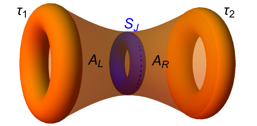
(a)

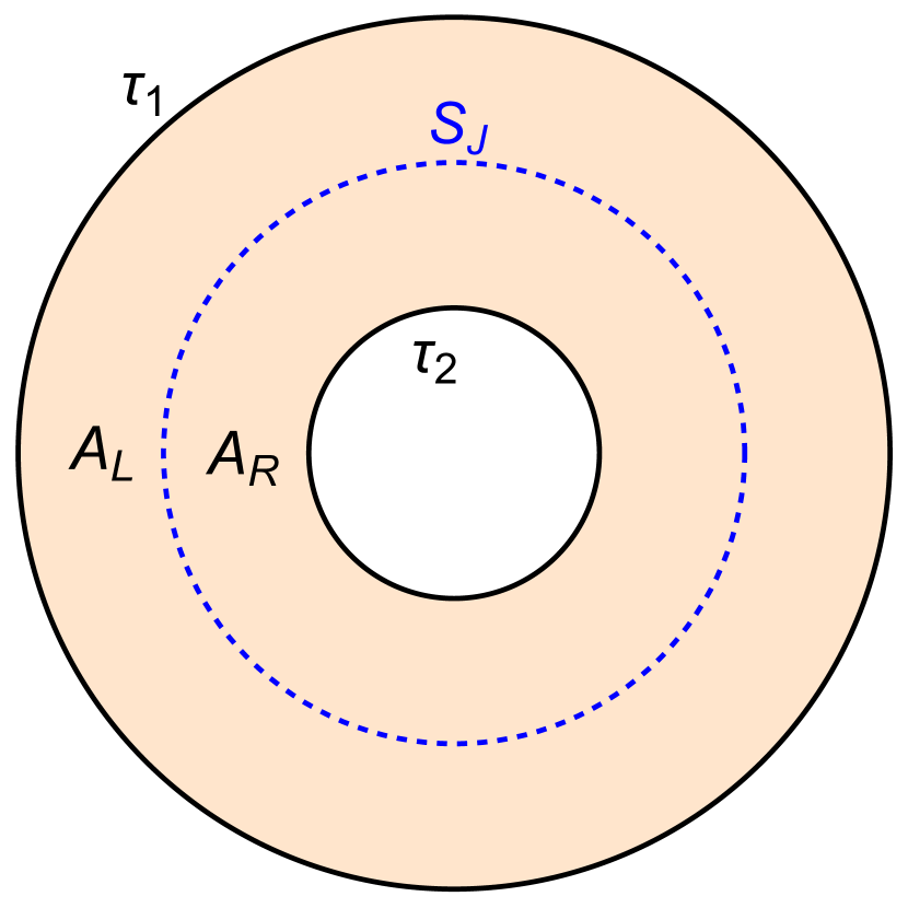
(b)

Figure 2: Wormhole geometry $T^{2}\times I$ with inclusion of the surface defect $\mathcal{S}_{J}$ along the non trivial 2-cycle in the bulk. In (a) the $I$ radial factor is displayed as connecting the two boundary components. In (b) only the ‘spatial’ annulus slice is displayed (the compact ‘Euclidean time’  direction is perpendicular to the paper). $\tau_{1}$ and $\tau_{2}$ denote the two boundary complex moduli, while $A_{L}$ and $A_{R}$ are the gauge fields on the two sides of the defect.

$$\left(\frac{k}{\pi}\oint A_{L}\right)-\omega_{J}\left(\frac{k}{\pi}\oint A_{R}\right)=0\mod\frac{2k}{\alpha_{J}}$$ (124)

whenever $i_{L,R}:=\frac{k}{\pi}\oint A_{L,R}$ are divisible by $\alpha_{J}$ (here $A_{L,R}$ are the gauge fields on the two sides of $\mathcal{S}_{J}$). In terms of the divisor $\delta_{J}$ associated to $\omega_{J}$, this can be equivalently rewritten as

$$\frac{k}{\pi}\oint(A_{L}-A_{R})|_{\mathcal{S}}=0\mod\frac{2k}{\delta_{J}},\qquad\frac{k}{\pi}\oint(A_{L}+A_{R})|_{\mathcal{S}}=0\mod 2\delta_{J}.$$ (125)

Notice that since the sewing conditions are topological they do not break diffeomorphism invariance, hence their insertions produce quantities which are invariant under diagonal modular transformations, by the same argument as given below (26). Moreover when $\omega_{J}$ is taken to be the identity we are describing a trivial or invisible defect, and the path integral agrees with the bilinear diagonal modular invariant (34).

The surface $\mathcal{S}_{J}$ with sewing conditions enforcing (125) can be precisely identified as a topological defect of the type introduced in Kapustin:2010if . Their full analysis from a Lagrangian point of view requires some more care than what we explained above, we refer also to Roumpedakis_2023 for a recent detailed review. It is now clear that the terms with $J\neq 1$ in the seed amplitude (123) arise from path integrals with insertions of nontrivial surface defects.

For completeness we notice that these surfaces could alternatively be introduced using the so called ‘folding trick’ (see Figure 3):

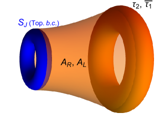
Figure 3: Folding trick. The wormhole geometry of Fig. 2.a has been ‘folded’ along the surface defect, which now behaves as a topological boundary condition. Due to orientation reversing one of the two sides, the theory has gauge group $U(1)_{k}\times U(1)_{-k}$ and one of the boundary conditions has been conjugated.

one considers a ‘folded’ $U(1)_{k}\times U(1)_{-k}$ Chern-Simons theory on the torus times an interval $[0,1]$ whith dynamical boundary conditions on $T^{2}\times\{0\}$ fixing modular parameters $\tau_{1}$ and $\tau_{2}$ for the two gauge fields, and topological boundary conditions on $T^{2}\times\{1\}$ that essentially relate the holonomies of the two gauge fields as in (125) (up to orientation). The path integral then picks a state on the Hilbert space at $T^{2}\times\{0\}$, which is invariant under large diffeomorphisms (diagonal modular transformations on $\tau_{1},\tau_{2}$) because the boundary conditions at $T^{2}\times\{1\}$ are topological. Reversing the orientation of one of the two $U(1)$ theories makes the above construction equivalent to the ‘unfolded’ $U(1)_{k}$ theory on $T^{2}\times[0,2]$, where the two opposite boundaries have dynamical boundary conditions and the topological boundary conditions at $S=T^{2}\times\{1\}$ are interpreted as sewing conditions on the topological defect.

On general grounds, two topological surface defects can be fused together to form a new defect. This fusion gives the set of defects the structure of a monoid, since the inverse is not guaranteed to exist, with the trivial defect playing the role of a unit element. The particular fusion rule found in Kapustin:2010if is

$$\mathcal{S}_{I}\circ\mathcal{S}_{J} =\gcd\left(\delta_{I},\delta_{J},\frac{k}{\delta_{I}},\frac{k}{\delta_{J}}\right)\mathcal{S}_{K(I,J)},$$ (126)

$$\text{where}\quad\delta_{K(I,J)} :=\mathrm{lcm}\left(\gcd\left(\delta_{I},\frac{k}{\delta_{J}}\right),\gcd\left(\delta_{J},\frac{k}{\delta_{I}}\right)\right).$$

From the above considerations, the fusion of the defects should agree with the monoidal structure (60) of the modular invariant matrices $M_{J}$ under multiplication. It is a heartening consistency check to indeed verify this, as we do in Appendix A.

6 Discussion

In this paper we have analyzed the implications of the requirement that the 2-boundary bulk amplitude should capture the variance of the ensemble distribution, under the plausible assumptions that it comes from a seed amplitude $Z^{(1)}_{\rm seed}$ which is holomorphically factorized (25) and satisfies the Cotler-Jensen property (26). We focused on ensembles of rational compact boson CFTs, and were able to analyze the problem in general when the level $k$ is square-free.

6.1 Some lessons

Let us summarize the results of this analysis and some lessons we can draw from them. When the ensemble consists of more than two CFTs, i.e. when the level $k$ is not a prime number, we found that the consistency constraints (31) are highly constraining and allow for only two possibilities.

A first and somewhat trivial possibility occurs when we start with a 1-boundary seed amplitude which is already modular invariant by itself; this picks out a specific CFT and, as here is no ensemble, the wormhole coefficients $c_{I}$ all vanish. This can be thought of as starting from a UV-complete complete theory and illustrates how the ensemble averaging phenomenon is related to effective gravity theories which are not UV complete. This situation is similar to e.g. tensionless string theory on AdS₃, which has a seed amplitude which is already modular invariant Eberhardt:2021jvj . As discussed in Benini:2022hzx , starting from a modular invariant seed amplitude can also interpreted as gauging a non-anomalous global 1-form symmetry, and is consistent with the expectation that global symmetries should be absent in a UV-complete theory of gravity.

The second possibility leads to an ensemble with maximal entropy and uniform ensemble weights. It is reassuring that this possibility also arises from the most natural starting point, where the 1-boundary seed amplitude is simply the pure Chern-Simons path-integral on the solid torus. Interestingly, the same ensemble could be obtained from the charge-$k$ excited state $\tilde{\chi}_{k}$.

Modulo this last subtlety, it is interesting that the consistent starting points are in some sense either fully UV complete or a maximally UV-ignorant, containing only the vacuum, and that intermediate starting points, such as a $Z^{(1)}_{\rm seed}$ containing the vacuum plus a few additional matter representations, are not consistent.

Another conclusion we reached is that in none of the examined cases the wormhole coefficients agree with the naive answer (35) given by the pure Chern-Simons path integral. In the models which describe an ensemble, we found that it is always necessary to include additional contributions from exotic wormholes, which are realized as a path integral in the presence of a Kapustin-Saulina surface defect. In the examples describing a single CFT, which include the $k=1$ case and the UV-complete theories, the wormhole coefficients vanish. This means that in these cases, we are instructed not to include two-boundary geometries in the path integral, lest we get an inconsistent result. This is perhaps similar to string theory on AdS${}_{5}\times$S⁵, where wormhole saddle points exist in the low-energy approximation Maldacena:2004rf which should most likely not be included in the path integral.

6.2 Outlook

Let us end by discussing some open problems and possible generalizations. Perhaps the biggest question raised by our analysis is if the 2-boundary seed amplitude, derived here from requiring a consistent holographic description of the ensemble, can be given an intrinsic three-dimensional geometric meaning. Our arguments showed that the two-boundary path integral should be performed with the insertion of a formal combination $\oplus_{I}(c_{I}{\cal S}_{I})$ of surface defects, and it would be interesting if this prescription could be given a physical interpretation, for example as arising from gauging a certain global symmetry. Such insights would go a long way to generalize our work to determining the seed amplitudes for multi-boundary amplitudes and higher genus boundaries. It will be interesting to see if the uniform ensemble distribution arising from the vacuum seed will pass the consistency tests arising on these topologies as well.

An obvious question is how our work generalizes to the holographic description of ensembles in other rational CFTs. A first class to consider would be the rational boson ensembles in which $k$ has nontrivial square divisors. As we saw above, the additional complications stem, on the boundary side, from the fact that the chiral algebra extends or, in the bulk, from the existence of non-invertible zero-form symmetries associated to certain surface defects. We briefly touched on this class of theories in the suggestive example in par. 4.1.4, and a general analysis is in progress Paolo . Also of interest would be the generalization to multiple compact bosons in rational Narain theories (see Furuta:2023xwl for a classification) and to Wess-Zumino-Witten models as well as Virasoro minimal models. As a by-product it would be interesting to harness the existing knowledge of modular invariants through their ADE classification Cappelli:1987xt to holographically determine or verify the fusion rules of surface defects in the associated Chern-Simons theories. In the interest of understanding the Euclidean path integral in more general contexts like Penington:2019kki ; Almheiri:2019qdq , it would also be desirable give a clear bulk path-integral derivation of the partition function on the torus times an interval with the insertion of a surface defect, following related recent studies Porrati:2019knx ; Porrati:2021sdc .

In order to progress towards the ultimate goal of understanding the ensemble interpretation of pure 3D gravity, we should extend the analysis of multi-boundary consistency constraints to ensembles of irrational CFTs. A natural first step would be to consider the Narain ensembles of irrational free boson theories Afkhami-Jeddi:2020ezh ; Maloney:2020nni . In this case, the required Poincaré-summed ‘exotic wormhole’ contributions were determined in Collier:2021rsn , and it would be of interest to see if those arise form a sensible seed amplitude and allow for an interpretation in terms of surface defects. The current work may also shed light on the ensemble description of pure gravity at certain negative values of the central charge Raeymaekers:2020gtz ; Campoleoni:2017xyl , where the chiral algebra has been argued to be a twisted version of the rational boson algebra ${\cal A}_{k}$.

Appendix A Fusion rules of surface defects

The surface defects of Kapustin:2010if are parametrized by the divisors of the level $k$. Given two divisors $\delta_{I},\delta_{J}$, the fusion of the associated defects $\mathcal{S}_{I}$ and $\mathcal{S}_{J}$ is governed by the rule

$$\mathcal{S}_{I}\circ\mathcal{S}_{J}=G\left(\delta_{I},\delta_{J},\frac{k}{\delta_{I}},\frac{k}{\delta_{J}}\right)\mathcal{S}_{K(I,J)},\qquad\delta_{K(I,J)}:=L\left(G\left(\delta_{I},\frac{k}{\delta_{J}}\right),G\left(\delta_{J},\frac{k}{\delta_{I}}\right)\right).$$ (127)

In this Section we show the agreement between this formula and the multiplication rule (60) satisfied by the modular invariant matrices $M_{I}$.

First of all we notice that, by definition of $\alpha_{I}=G(\delta_{I},k/\delta_{I})$ and associativity of gcd, the prefactors agree:

$$G\left(\delta_{I},\delta_{J},\frac{k}{\delta_{I}},\frac{k}{\delta_{J}}\right)=G\left(\alpha_{I},\alpha_{J}\right).$$ (128)

Now we will rewrite the formula for $\delta_{K(I,J)}$ in a more suitable form. Using standard properties of gcd and lcm one can show that

$$G(\delta_{I},\delta_{J})G\left(\delta_{I},\frac{k}{\delta_{J}}\right)=\delta_{I}G\left(\delta_{I},\delta_{J},\frac{k}{L(\delta_{I},\delta_{J})}\right)=\delta_{I}G(\alpha_{I},\alpha_{J}).$$ (129)

Thus, collecting $\frac{G(\alpha_{I},\alpha_{J})}{G(\delta_{I},\delta_{J})}$, (127) can be rewritten as

$$\delta_{K(I,J)}=\frac{G(\alpha_{I},\alpha_{J})L(\delta_{I},\delta_{J})}{G(\delta_{I},\delta_{J})}.$$ (130)

To compare with the multiplication law (61), we must show that

$$\delta_{K(I,J)}\stackrel{{\scriptstyle?}}{{=}}\delta(\omega_{I}\bullet\omega_{J})=L(\alpha_{I},\alpha_{J})G\left(\frac{\omega_{I}\omega_{J}+1}{2},\frac{k}{L(\alpha_{I},\alpha_{J})^{2}}\right),$$ (131)

where we used (64) on the RHS.

Starting from the RHS, we multiply and divide by $G(\delta_{I},\delta_{J})$, use distributivity and associativity of the gcd and replace $\delta_{I}=\delta(\omega_{I})=\alpha_{I}G\left(\frac{\omega_{I}+1}{2},\frac{k}{\alpha_{I}^{2}}\right)$ to get

$$\delta(\omega_{I}\bullet\omega_{J})=\frac{L(\alpha_{I},\alpha_{J})}{G(\delta_{I},\delta_{J})}G\left(\delta_{I}\frac{\omega_{I}\omega_{J}+1}{2},\delta_{J}\frac{\omega_{I}\omega_{J}+1}{2},\delta_{I}\frac{k}{L(\alpha_{I},\alpha_{J})^{2}},\delta_{J}\frac{k}{L(\alpha_{I},\alpha_{J})^{2}}\right)$$ (132)

$$=\frac{L(\alpha_{I},\alpha_{J})}{G(\delta_{I},\delta_{J})}G\Bigg{(}\alpha_{I}\frac{\omega_{I}+1}{2}\frac{\omega_{I}\omega_{J}+1}{2},\alpha_{J}\frac{\omega_{J}+1}{2}\frac{\omega_{I}\omega_{J}+1}{2},$$

$$\qquad\underbrace{\frac{k}{L(\alpha_{I},\alpha_{J})}\frac{\omega_{I}\omega_{J}+1}{2},\alpha_{I}\frac{\omega_{I}+1}{2}\frac{k}{L(\alpha_{I},\alpha_{J})^{2}},\alpha_{J}\frac{\omega_{J}+1}{2}\frac{k}{L(\alpha_{I},\alpha_{J})^{2}},\frac{k^{2}}{L(\alpha_{I},\alpha_{J})^{3}}}_{(*)}\Bigg{)}.$$

Let us focus on $(*)$. Rewriting $\frac{\omega_{I}\omega_{J}+1}{2}=\omega_{I}\frac{\omega_{J}+1}{2}+\frac{1-\omega_{J}}{2}$, noticing that $\alpha_{I}\frac{\omega_{I}+1}{2}$ and repeatedly using standard properties of the gcd one can see that

$$(*)=G\left(\frac{k}{L(\alpha_{I},\alpha_{J})},\alpha_{I}\frac{\omega_{I}+1}{2}\frac{k}{L(\alpha_{I},\alpha_{J})^{2}},\alpha_{J}\frac{\omega_{J}+1}{2}\frac{k}{L(\alpha_{I},\alpha_{J})^{2}}\right).$$ (133)

Notice that $\alpha_{I}\frac{\omega_{I}+1}{2}\frac{\omega_{I}\omega_{J}+1}{2}=\alpha_{I}\frac{\omega_{I}+1}{2}\frac{\omega_{J}+1}{2}+2\omega_{J}M\frac{k}{\alpha_{I}}$ for some integer $M$ satisfying $\omega_{I}^{2}=1+M(4k/\alpha_{I}^{2})$ (and analogously for $\omega_{J}$). Since in the main expression we work modulo $\frac{k}{L(\alpha_{I},\alpha_{J})}$, we can substitute $\alpha_{I}\frac{\omega_{I}+1}{2}\frac{\omega_{I}\omega_{J}+1}{2}\sim\alpha_{I}\frac{\omega_{I}+1}{2}\frac{\omega_{J}+1}{2}$:

$$\delta_{I}(\omega_{I}\bullet\omega_{J}) =\frac{L(\alpha_{I},\alpha_{J})}{G(\delta_{I},\delta_{J})}G\Bigg{(}G(\alpha_{I},\alpha_{J})\frac{\omega_{I}+1}{2}\frac{\omega_{J}+1}{2},\frac{k}{L(\alpha_{I},\alpha_{J})},$$ (134)

$$\qquad\qquad\qquad\qquad\qquad\alpha_{I}\frac{\omega_{I}+1}{2}\frac{k}{L(\alpha_{I},\alpha_{J})^{2}},\alpha_{J}\frac{\omega_{J}+1}{2}\frac{k}{L(\alpha_{I},\alpha_{J})^{2}}\Bigg{)}$$

$$=\frac{1}{G(\delta_{I},\delta_{J})}G\left(\alpha_{I}\frac{\omega_{I}+1}{2}\alpha_{J}\frac{\omega_{J}+1}{2},k,\alpha_{I}\frac{\omega_{I}+1}{2}\frac{k}{L(\alpha_{I},\alpha_{J})},\alpha_{J}\frac{\omega_{J}+1}{2}\frac{k}{L(\alpha_{I},\alpha_{J})}\right)$$

where we used $G(\alpha_{I},\alpha_{J})L(\alpha_{I},\alpha_{J})=\alpha_{I}\alpha_{J}$. Now using the definition of $\delta(\omega)$ we substitute $\alpha\frac{\omega+1}{2}=R\delta$, where $R$ is an integer satisfying $G(R,k/\alpha)=G(R,\alpha)=G(R,k)=1$. Since under the gcd we can work modulo $k$, both $R_{I}$ and $R_{J}$ can be simplified, leading to

$$=\frac{1}{G(\delta_{I},\delta_{J})}G\Bigg{(}\underbrace{\delta_{I}\delta_{J},k}_{=L(\delta_{I},\delta_{J})G(\alpha_{I},\alpha_{J})},\underbrace{\frac{k}{L(\alpha_{I},\alpha_{J})}\delta_{I},\frac{k}{L(\alpha_{I},\alpha_{J})}\delta_{J}}_{=\frac{k}{L(\alpha_{I},\alpha_{J})}G(\delta_{I},\delta_{J})}\Bigg{)}$$ (135)

$$=\frac{G(\alpha_{I},\alpha_{J})}{G(\delta_{I},\delta_{J})}G\left(L(\delta_{I},\delta_{J}),\frac{k}{\alpha_{I}\alpha_{J}}G(\delta_{I},\delta_{J})\right).$$

Using prime decomposition we will check below that $L(\delta_{I},\delta_{J})$ divides $\frac{k}{\alpha_{I}\alpha_{J}}G(\delta_{I},\delta_{J})$, hence the final result is

$$\delta_{I}(\omega_{I}\bullet\omega_{J})=\frac{G(\alpha_{I},\alpha_{J})L(\delta_{I},\delta_{J})}{G(\delta_{I},\delta_{J})}=\delta_{K(I,J)}$$ (136)

as desired.

Let us check the promised relation $G\left(L(\delta_{I},\delta_{J}),\frac{k}{\alpha_{I}\alpha_{J}}G(\delta_{I},\delta_{J})\right)=L(\delta_{I},\delta_{J})$. Fix the prime decompositons

$$k=\prod_{j}p_{j}^{n_{j}},\qquad\delta_{I}=\prod_{j}p_{j}^{m_{j}},\qquad\delta_{J}=\prod_{j}p_{j}^{\tilde{m}_{j}},$$ (137)

with $m_{j},\tilde{m}_{j}\leq n_{j}$. Then $\alpha_{I}=\prod_{j}p_{j}^{\min(m_{j},n_{j}-m_{j})}$, $\alpha_{J}=\prod_{j}p_{j}^{\min(\tilde{m}_{j},n_{j}-\tilde{m}_{j})}$ and $L(\delta_{I},\delta_{J})=\prod_{j}p_{j}^{\max(m_{j},\tilde{m}_{j})}$. Also the other combination in the gcd is

$$\frac{k}{\alpha_{I}\alpha_{J}}G(\delta_{I},\delta_{J})=\prod_{j}p_{j}^{n_{j}+\min(m_{j},\tilde{m}_{j})-\min(m_{j},n_{j}-m_{j})-\min(\tilde{m}_{j},n_{j}-\tilde{m}_{j})}.$$ (138)

For each $j$, the exponents in this last expression can be explicitly seen to satisfy

$$n+\min(m,\tilde{m})-\min(m,n-m)-\min(\tilde{m},n-\tilde{m})\geq\begin{cases}m&m>\tilde{m}\\ \tilde{m}&m<\tilde{m}\end{cases}.$$ (139)

The RHS is the form of the exponents of $L(\delta_{I},\delta_{J})$, hence the latter divides $\frac{k}{\alpha_{I}\alpha_{J}}G(\delta_{I},\delta_{J})$ as claimed.

References

- (1) G. Penington, S. H. Shenker, D. Stanford, and Z. Yang, “Replica wormholes and the black hole interior,” JHEP 03 (2022) 205, arXiv:1911.11977 [hep-th].
- (2) A. Almheiri, T. Hartman, J. Maldacena, E. Shaghoulian, and A. Tajdini, “Replica Wormholes and the Entropy of Hawking Radiation,” JHEP 05 (2020) 013, arXiv:1911.12333 [hep-th].
- (3) P. Saad, S. H. Shenker, and D. Stanford, “JT gravity as a matrix integral,” arXiv:1903.11115 [hep-th].
- (4) A. Maloney and E. Witten, “Quantum Gravity Partition Functions in Three Dimensions,” JHEP 02 (2010) 029, arXiv:0712.0155 [hep-th].
- (5) J. Cotler and K. Jensen, “AdS3 gravity and random CFT,” JHEP 04 (2021) 033, arXiv:2006.08648 [hep-th].
- (6) C. A. Keller and A. Maloney, “Poincare Series, 3D Gravity and CFT Spectroscopy,” JHEP 02 (2015) 080, arXiv:1407.6008 [hep-th].
- (7) N. Benjamin, H. Ooguri, S.-H. Shao, and Y. Wang, “Light-cone modular bootstrap and pure gravity,” Phys. Rev. D 100 no. 6, (2019) 066029, arXiv:1906.04184 [hep-th].
- (8) N. Benjamin, S. Collier, and A. Maloney, “Pure Gravity and Conical Defects,” JHEP 09 (2020) 034, arXiv:2004.14428 [hep-th].
- (9) H. Maxfield and G. J. Turiaci, “The path integral of 3D gravity near extremality; or, JT gravity with defects as a matrix integral,” JHEP 01 (2021) 118, arXiv:2006.11317 [hep-th].
- (10) N. Afkhami-Jeddi, H. Cohn, T. Hartman, and A. Tajdini, “Free partition functions and an averaged holographic duality,” JHEP 01 (2021) 130, arXiv:2006.04839 [hep-th].
- (11) A. Maloney and E. Witten, “Averaging over Narain moduli space,” JHEP 10 (2020) 187, arXiv:2006.04855 [hep-th].
- (12) A. Pérez and R. Troncoso, “Gravitational dual of averaged free CFT’s over the Narain lattice,” JHEP 11 (2020) 015, arXiv:2006.08216 [hep-th].
- (13) A. Dymarsky and A. Shapere, “Comments on the holographic description of Narain theories,” JHEP 10 (2021) 197, arXiv:2012.15830 [hep-th].
- (14) S. Datta, S. Duary, P. Kraus, P. Maity, and A. Maloney, “Adding flavor to the Narain ensemble,” JHEP 05 (2022) 090, arXiv:2102.12509 [hep-th].
- (15) N. Benjamin, C. A. Keller, H. Ooguri, and I. G. Zadeh, “Narain to Narnia,” Commun. Math. Phys. 390 no. 1, (2022) 425–470, arXiv:2103.15826 [hep-th].
- (16) M. Ashwinkumar, M. Dodelson, A. Kidambi, J. M. Leedom, and M. Yamazaki, “Chern-Simons invariants from ensemble averages,” JHEP 08 (2021) 044, arXiv:2104.14710 [hep-th].
- (17) J. Dong, T. Hartman, and Y. Jiang, “Averaging over moduli in deformed WZW models,” JHEP 09 (2021) 185, arXiv:2105.12594 [hep-th].
- (18) S. Collier and A. Maloney, “Wormholes and spectral statistics in the Narain ensemble,” JHEP 03 (2022) 004, arXiv:2106.12760 [hep-th].
- (19) N. Benjamin, S. Collier, A. L. Fitzpatrick, A. Maloney, and E. Perlmutter, “Harmonic analysis of 2d CFT partition functions,” JHEP 09 (2021) 174, arXiv:2107.10744 [hep-th].
- (20) A. Dymarsky and A. Sharon, “Non-rational Narain CFTs from codes over F4,” JHEP 11 (2021) 016, arXiv:2107.02816 [hep-th].
- (21) S. Chakraborty and A. Hashimoto, “Weighted average over the Narain moduli space as a TTbar deformation of the CFT target space,” Phys. Rev. D 105 no. 8, (2022) 086018, arXiv:2109.10382 [hep-th].
- (22) J. Henriksson, A. Kakkar, and B. McPeak, “Narain CFTs and quantum codes at higher genus,” JHEP 04 (2023) 011, arXiv:2205.00025 [hep-th].
- (23) K. Kawabata, T. Nishioka, and T. Okuda, “Narain CFTs from qudit stabilizer codes,” SciPost Phys. Core 6 (2023) 035, arXiv:2212.07089 [hep-th].
- (24) J. Kames-King, A. Kanargias, B. Knighton, and M. Usatyuk, “The Lion, the Witch, and the Wormhole: Ensemble averaging the symmetric product orbifold,” arXiv:2306.07321 [hep-th].
- (25) Y. F. Alam, K. Kawabata, T. Nishioka, T. Okuda, and S. Yahagi, “Narain CFTs from nonbinary stabilizer codes,” arXiv:2307.10581 [hep-th].
- (26) K. Kawabata, T. Nishioka, and T. Okuda, “Supersymmetric conformal field theories from quantum stabilizer codes,” Phys. Rev. D 108 no. 8, (2023) L081901, arXiv:2307.14602 [hep-th].
- (27) K. Kawabata, T. Nishioka, and T. Okuda, “Narain CFTs from quantum codes and their gauging,” arXiv:2308.01579 [hep-th].
- (28) O. Aharony, A. Dymarsky, and A. D. Shapere, “Holographic description of Narain CFTs and their code-based ensembles,” arXiv:2310.06012 [hep-th].
- (29) M. Ashwinkumar, A. Kidambi, J. M. Leedom, and M. Yamazaki, “Generalized Narain Theories Decoded: Discussions on Eisenstein series, Characteristics, Orbifolds, Discriminants and Ensembles in any Dimension,” arXiv:2311.00699 [hep-th].
- (30) V. Meruliya, S. Mukhi, and P. Singh, “Poincaré Series, 3d Gravity and Averages of Rational CFT,” JHEP 04 (2021) 267, arXiv:2102.03136 [hep-th].
- (31) A. Castro, M. R. Gaberdiel, T. Hartman, A. Maloney, and R. Volpato, “The Gravity Dual of the Ising Model,” Phys. Rev. D 85 (2012) 024032, arXiv:1111.1987 [hep-th].
- (32) V. Meruliya and S. Mukhi, “AdS3 gravity and RCFT ensembles with multiple invariants,” JHEP 08 (2021) 098, arXiv:2104.10178 [hep-th].
- (33) I. Romaidis and I. Runkel, “CFT correlators and mapping class group averages,” arXiv:2309.14000 [hep-th].
- (34) J. Henriksson, A. Kakkar, and B. McPeak, “Classical codes and chiral CFTs at higher genus,” JHEP 05 (2022) 159, arXiv:2112.05168 [hep-th].
- (35) M. Buican, A. Dymarsky, and R. Radhakrishnan, “Quantum codes, CFTs, and defects,” JHEP 03 (2023) 017, arXiv:2112.12162 [hep-th].
- (36) F. Benini, C. Copetti, and L. Di Pietro, “Factorization and global symmetries in holography,” SciPost Phys. 14 no. 2, (2023) 019, arXiv:2203.09537 [hep-th].
- (37) J. Henriksson and B. McPeak, “Averaging over codes and an SU(2) modular bootstrap,” JHEP 11 (2023) 035, arXiv:2208.14457 [hep-th].
- (38) J. Raeymaekers, “A note on ensemble holography for rational tori,” JHEP 12 (2021) 177, arXiv:2110.08833 [hep-th].
- (39) J. Cotler and K. Jensen, “AdS3 wormholes from a modular bootstrap,” JHEP 11 (2020) 058, arXiv:2007.15653 [hep-th].
- (40) S. Elitzur, G. W. Moore, A. Schwimmer, and N. Seiberg, “Remarks on the Canonical Quantization of the Chern-Simons-Witten Theory,” Nucl. Phys. B 326 (1989) 108–134.
- (41) J. Cotler and K. Jensen, “A theory of reparameterizations for AdS3 gravity,” JHEP 02 (2019) 079, arXiv:1808.03263 [hep-th].
- (42) A. Kapustin and N. Saulina, “Surface operators in 3d Topological Field Theory and 2d Rational Conformal Field Theory,” arXiv:1012.0911 [hep-th].
- (43) J. Fuchs, I. Runkel, and C. Schweigert, “TFT construction of RCFT correlators 1. Partition functions,” Nucl. Phys. B 646 (2002) 353–497, arXiv:hep-th/0204148.
- (44) S. Choudhury and K. Shirish, “Wormhole calculus without averaging from O(N)q-1 tensor model,” Phys. Rev. D 105 no. 4, (2022) 046002, arXiv:2106.14886 [hep-th].
- (45) J. J. Heckman, A. P. Turner, and X. Yu, “Disorder averaging and its UV discontents,” Phys. Rev. D 105 no. 8, (2022) 086021, arXiv:2111.06404 [hep-th].
- (46) F. Baume, J. J. Heckman, M. Hübner, E. Torres, A. P. Turner, and X. Yu, “SymTrees and Multi-Sector QFTs,” arXiv:2310.12980 [hep-th].
- (47) G. W. Moore and N. Seiberg, “Taming the Conformal Zoo,” Phys. Lett. B 220 (1989) 422–430.
- (48) G. W. Moore and N. Seiberg, “Naturality in Conformal Field Theory,” Nucl. Phys. B 313 (1989) 16–40.
- (49) J. M. Maldacena and A. Strominger, “AdS(3) black holes and a stringy exclusion principle,” JHEP 12 (1998) 005, arXiv:hep-th/9804085.
- (50) J. Polchinski, String theory. Vol. 1: An introduction to the bosonic string. Cambridge Monographs on Mathematical Physics. Cambridge University Press, 12, 2007.
- (51) P. Di Francesco, P. Mathieu, and D. Senechal, Conformal Field Theory. Graduate Texts in Contemporary Physics. Springer-Verlag, New York, 1997.
- (52) P. Kraus and F. Larsen, “Partition functions and elliptic genera from supergravity,” JHEP 01 (2007) 002, arXiv:hep-th/0607138.
- (53) A. Cappelli, C. Itzykson, and J. B. Zuber, “Modular Invariant Partition Functions in Two-Dimensions,” Nucl. Phys. B 280 (1987) 445–465.
- (54) A. Cappelli, C. Itzykson, and J. B. Zuber, “The ADE Classification of Minimal and A1(1) Conformal Invariant Theories,” Commun. Math. Phys. 113 (1987) 1.
- (55) R. Omami, M. Omami, and R. Ouni, “Group of square roots of unity modulo n,” International Journal of Mathematical and Computational Sciences 3 no. 7, (2009) 505 – 513.
- (56) A. Kapustin and N. Saulina, “Topological boundary conditions in abelian Chern-Simons theory,” Nucl. Phys. B 845 (2011) 393–435, arXiv:1008.0654 [hep-th].
- (57) K. Roumpedakis, S. Seifnashri, and S.-H. Shao, “Higher gauging and non-invertible condensation defects,” Communications in Mathematical Physics 401 no. 3, (May, 2023) 3043–3107.
- (58) L. Eberhardt, “Summing over Geometries in String Theory,” JHEP 05 (2021) 233, arXiv:2102.12355 [hep-th].
- (59) J. M. Maldacena and L. Maoz, “Wormholes in AdS,” JHEP 02 (2004) 053, arXiv:hep-th/0401024.
- (60) w. i. p. Paolo Rossi.
- (61) Y. Furuta, “On the Rationality and the Code Structure of a Narain CFT, and the Simple Current Orbifold,” arXiv:2307.04190 [hep-th].
- (62) M. Porrati and C. Yu, “Kac-Moody and Virasoro Characters from the Perturbative Chern-Simons Path Integral,” JHEP 05 (2019) 083, arXiv:1903.05100 [hep-th].
- (63) M. Porrati and C. Yu, “Partition functions of Chern-Simons theory on handlebodies by radial quantization,” JHEP 07 (2021) 194, arXiv:2104.12799 [hep-th].
- (64) J. Raeymaekers, “Conical spaces, modular invariance and holography,” JHEP 03 (2021) 189, arXiv:2012.07934 [hep-th].
- (65) A. Campoleoni, S. Fredenhagen, and J. Raeymaekers, “Quantizing higher-spin gravity in free-field variables,” JHEP 02 (2018) 126, arXiv:1712.08078 [hep-th].