Entanglement production from scattering of fermionic wave packets: a quantum computing approach
Abstract
We propose a method to prepare Gaussian wave packets with momentum on top of the interacting ground state of a fermionic Hamiltonian. Using Givens rotation, we show how to efficiently obtain expectation values of observables throughout the evolution of the wave packets on digital quantum computers. We demonstrate our technique by applying it to the staggered lattice formulation of the Thirring model and studying the scattering of two wave packets. Monitoring the the particle density and the entropy produced during the scattering process, we characterize the phenomenon and provide a first step towards studying more complicated collision processes on digital quantum computers. In addition, we perform a small-scale demonstration on IBM’s quantum hardware, showing that our method is suitable for current and near-term quantum devices.
I Introduction
Collider experiments play a central role for understanding the subatomic structure of matter, and for developing and verifying the theoretical description of the elementary particles and their interactions. Arguably, the most prominent example is the LHC at CERN, which enabled a major experimental breakthrough with the discovery of the Higgs boson [1, 2]. While the Standard Model provides a theoretical description for all known elementary particles and the fundamental forces among them (except for gravity) in terms of gauge theories, the understanding of scattering processes and more general out-of-equilibrium dynamics at a fundamental level remains challenging. In particular, these phenomena are nonperturbative, and a standard tool for exploring this regime is lattice field theory. Discretizing the theory on a lattice allows for sophisticated Markov chain Monte Carlo simulations that have been highly successful for exploring static properties of gauge theories [3, 4]. However, the sign problem prevents an extension of this approach to dynamical problems, leaving open many relevant questions regarding the real-time evolution of scattering processes. Hence, there is an ongoing effort to find alternative approaches allowing for overcoming this limitation [5, 6, 7, 8].
Methods originating from quantum information theory provide a promising avenue towards studying real-time dynamics of lattice field theories. On the one hand, classical computational methods based on Tensor Networks have been demonstrated to allow for reliable simulations in regimes where conventional Monte Carlo methods suffer from the sign problem [9, 7]. Tensor Network states are a family of entanglement-based ansätze for the wave function of a strongly-correlated quantum many-body system, which allow for an efficient classical description of the system in case the entanglement in the system is not too large [10, 11, 12]. In particular, Tensor Network states were successfully used to study real-time dynamics of various (1+1)-dimensional Abelian and non-Abelian lattice gauge theories [13, 14], including meson scattering in the Schwinger model [15]. So far, Tensor Networks have been most successful for (1+1)-dimensional theories. Generalizing this success to higher dimensions is not an immediate task, although there already exist calculations for gauge models in higher dimensions [16, 17]. Moreover, the Tensor Network approach becomes inefficient in situations in which the entanglement in the system can become large. A prominent example are out-of-equilibrium dynamics following a global quench, during which the entanglement in the system can grow linearly in time [18, 19, 20]. Hence, for these problems only short to intermediate time-scales are accessible with Tensor Networks [21, 22].
On the other hand, quantum computers hold the major promise to be able to efficiently simulate real-time dynamics of lattice field theories, even in regimes that are challenging for Tensor Network. This has already been successfully demonstrated in various proof-of-principle experiments [23, 24, 25]. Simulating scattering processes for lattice field theories on a quantum computer poses a number of particular challenges. Firstly, one has to be able to simulate the evolution of some initial state under the Hamiltonian describing the theory. Secondly, the particles of the theory are typically highly nontrivial objects, and preparing the qubits of a digital quantum device in an initial state that corresponds to two particles with momenta, such that they start to move towards each other and scatter is not an easy task.
In this paper we provide first steps towards addressing some of these challenges using a staggered lattice discretization of the Thirring model [26] as a test bed. Using Givens rotation [27, 28, 29], we show how to prepare localized wave packets with momentum on a digital quantum computer, such that they start moving during the evolution in time. Starting from the ground state of the Hamiltonian, which can be obtained by the variational quantum eigensolver (VQE) [30] or some other method, this allows us to simulate scattering between particles and antiparticles for fermionic models. Performing numerical simulations of the quantum system on a classical computer, we demonstrate the elastic scattering of the fermions and we examine the entropy production during the evolution in the Thirring model. The approach we demonstrate for the Thirring model can straightforwardly be generalized to arbitrary fermionic models.
The paper is organized as follows. In Sec. II, we introduce the staggered discretization for the Thirring model that we are studying. Subsequently, we show how to create Gaussian wave packets with appropriate momentum to make the two particles collide in Sec. III. Our numerical results demonstrating the procedure are shown in Sec. IV. Finally, we conclude in Sec. V and provide an outlook.
II Model system and lattice formulation
Here we consider the massive Thirring model in (1+1) dimensions. The continuum Lagrangian for this model reads [26, 31]
| (1) |
where is a two-component Dirac spinor, the bare fermion mass, and the dimensionless four-fermion coupling constant . The spinor components fulfill the usual anti-commutation relations for fermions: , , where label the components of the spinor. In (1+1) dimensions the index takes values 0 and 1, and the matrices correspond to two of the Pauli matrices , , up to a phase factor; in the following we choose to work with the representation , . For a positive value of the coupling , the model is known to exhibit an attractive force between fermions and antifermions [32].
In order to address the theory numerically on a quantum computer, we need to adopt a Hamiltonian lattice formulation of the model. Following Ref. [31], we choose to work with the Kogut-Susskind staggered formulation, where the components of the spinor are distributed to different lattice sites in order to avoid the doubling problem [33, 34]. For a periodic lattice with sites and spacing , the lattice discretization of the Thirring model reads [31]
| (2) | ||||
where with and is a single-component fermionic field on site , and we identify . The fermionic creation and annihilation operators satisfy the anti-commutation relations
| (3) |
Note that for the four-fermion interaction term in Eq. (2) vanishes, and the resulting Hamiltonian corresponds to a staggered discretization of free Dirac fermions, which is quadratic in the fermion fields111Since we are working with a staggered discretization that separates the two components of the Dirac spinor to the odd and even sublattices, is considered to be even.. Thus, this case can be solved with free-fermion techniques both analytically [35] or on a quantum device [36]. Moreover, in this limit, the interpretation of the staggered lattice discretization in terms of particles and antiparticles becomes more transparent. Occupied even sites contribute to the energy and, thus, can be interpreted as particles with mass . In contrast, occupied odd sites contribute to the energy and correspond to the Dirac sea. Empty odd sites hence represent to a hole in the Dirac sea, i.e. an antiparticle with mass [37].
As conventional qubit-based quantum hardware cannot directly address fermionic degrees of freedom, we choose to map them to spins using a Jordan-Wigner transformation [38]
| (4) |
where . Inserting the expression above into Eq. (2), we obtain the Hamiltonian in terms of Pauli matrices
| (5) | ||||
where we again identify , , and tensor products between operators are assumed. Note that the non-local Pauli-strings in the second line of Eq. (5) arise due to the periodic boundary conditions, and are a consequence of the Jordan-Wigner transformation of the terms wrapping around the boundary. For the rest of this paper, we consider without loss of generality .
III Simulating real-time dynamics of scattering on a digital quantum computer
Simulating the out-of-equilibrium dynamics following a particle collision is highly nontrivial task, which is to a large extent inaccessible with MC methods due to the sign problem. Thus, there has been an ongoing effort to utilize methods from quantum information theory to simulate real-time evolution of scattering processes [39, 15] using the Hamiltonian formulation. In order to be able to simulate scattering processes, the following steps have to be accomplished.
-
1.
Preparing the ground state of the Hamiltonian, , which we refer to as the vacuum state.
-
2.
Generating an initial state that corresponds to the vacuum state with two wave packets at arbitrary distance, which represent particles and antiparticles with appropriately chosen momenta.
-
3.
Performing a real-time evolution on the initial state such that the particles will propagate and interact with each other over time.
-
4.
Measuring relevant observables in the state .
Mature approaches exist for performing step 1 on current quantum hardware, e.g. by means of VQE [40] or by applying variational imaginary time evolution [41, 42]. Similarly, the real time simulation in step 3 can be simulated in general by trotterizing the evolution operator [43, 44] or by means of variational time evolution methods [45, 46, 44]. Moreover, step 4 can also be done efficiently on a quantum computer for local observables.
Here we focus on some aspects concerning the steps 2–4, and assume the ground state can be prepared with some unitary from the state corresponding to all qubits initialized in state such that . Section III.1 reports on the preparation of the initial state corresponding to two particles with opposite momenta. The procedure consists of two steps. First, we consider the free fermionic case corresponding to . In this case, the model can be solved analytically, which allows us to construct exact operators creating a wave packet for particles and antiparticles. While these operators generate true (anti)particles only in the non-interacting case, they will also provide a valid approximation for a particle in the interacting case. In Section III.2 we then discuss the implementation of these states on a quantum device and provide the corresponding circuits using Givens rotations entangling gates. The implementation of the quantum dynamics circuits is described in Section III.3, while Section III.4 reports on the calculation of the time-dependent observables.
III.1 Free Gaussian fermion and antifermion wave packets in the staggered encoding
Let us first consider the non-interacting case , for which Eq. (2) corresponds to the staggered discretization of free Dirac fermions. Our goal is to derive operators which create a localized particle or antiparticle in the form of a Gaussian wave packet with associated momentum, acting on the vacuum state. This can be easily done using the plane wave solutions of the theory in momentum space. Reference [15] solved the model analytically, and in the rest of this subsection we will briefly review their results and show the construction of Gaussian wave packets.
Note that Eq. (2) is invariant under translations by two lattice sites due to the staggered mass term. Thus, it can be solved using standard methods by first performing a Fourier transformation followed by a Bogoliubov transformation. Doing this, we obtain two sets of creation operators, and , in momentum space which correspond to the creation operators for particles and antiparticles with momenta . The plane wave solutions can be used to construct operators creating Gaussian wave packets. Their representation in momentum space is given by
| (6) |
where the coefficients are given by a Gaussian distribution
| (7) |
The normalization factor
| (8) |
ensures that is a probability density and . The operator ) will create a Gaussian wave packet with a mean momentum and width in momentum space, located around in real space.
The operators in momentum space , are related to the original annihilation and creation operators in real space as
| (9) | ||||
where
| (10) |
and is a projection operator defined as
| (11) |
This allows for obtaining an explicit representation of the operators creating a wave packet in position space,
| (12) |
where the normalized coefficients are given by
| (13) | ||||
Looking at Eq. (12), we see that () corresponds to a superposition of creation (annihilation) operators, thus showing that it creates a wave packet for particles (antiparticles). Note that the coefficients in Eq. (13) are again normalized, , hence corresponds to a probability density.
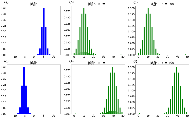
Focusing on the limit of infinite mass, , Eq. (10) reveals that for this case . Together with the properties of the projectors in Eq. (11), we see that in this limit () only affects the even (odd) sites. Thus, in this limit the particles are only located at the even sites whereas the antiparticles reside on the odd sites. For a finite mass one finds , hence the fermion and antifermion are located on both even and odd sites, with the amplitude of fermion (antifermion) being by suppressed the factor on odd (even) sites. Figure 1 illustrates this effect by showing the probability density in momentum and in position space for two values of the mass.
A state corresponding to the vacuum with a fermion and antifermion wave packet superimposed on top can now be obtained by acting with the operators and on the state with,
| (14) |
In order to prepare this state on a quantum device, one has to be able to implement the action of the operators and on a given fermionic state. In the following we discuss how this can be achieved with Givens rotations [27, 28, 29].
III.2 Givens rotation for preparing fermionic states
One of the most efficient ways to implement the action of linear combinations of the fermionic operators on a fermionic state is to use Givens rotations [27]. This approach allows for the realization of the resulting fermionic states with a quantum circuit of linear depth in the system size, [28, 29].
The linear combination of fermionic operators in Eq. (12) can be interpreted as a unitary transformation of the original creation and annihilation operators
| (15) |
where
| (16) |
with a unitary matrix . Choosing the first column of to be equal (), Eq. (15) corresponds exactly to the creation operators for Gaussian wave packets for fermion (antifermions) in Eq. (12). Note that this is always possible since and thus the can be interpreted as the entries of a complex unit vector in . Furthermore, since we do not care about the other columns of , we can simply choose these such that the columns of form an orthonormal basis of .
The map is a homomorphism under matrix multiplication, i.e. . Thus, in order to obtain a decomposition in in unitary gates that can be implemented on a quantum computer, we can decompose the matrix in a product of unitaries acting nontrivially only on a few sites. This can be done with Givens rotations [28, 29], as detailed in Appendix A. Since we care only about the first column of , corresponding to , we hereafter will write instead of .
In summary, we can decompose the matrix into a product of a diagonal matrix and Givens rotation matrices, , . This allows us to construct a decomposition of the operator using that it is a homomorphism under matrix multiplication. In particular, the structure of the Givens rotation matrices is such that acts non-trivially only on two neighboring sites. More specifically, if we write the complex Gaussian amplitudes in position space in polar form, , , with absolute value and phase angle , we can decompose the operator as,
| (17) |
In the expression above is a real vector whose entries are the phase angles of the Gaussian amplitudes and the terms correspond to
| (18) | ||||
| (19) |
where is the Givens rotation angle given by .
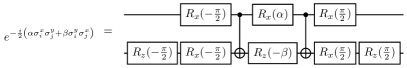
Using the Jordan-Wigner transformation from Eq. (4), the operator can be mapped to a set of single-qubit rotation gates (up to a global phase)
| (20) |
where is the standard Pauli rotation gate about the -axis. For the Jordan-Wigner transformation yields a particle-number conserving two-qubit gate
| (21) |
The two-qubit gate in Eq. (21) above can be easily expressed by single-qubit Pauli rotation gates, , , and CNOT gates as shown in Fig. 2.
Analogously, we can obtain an expression for and also decompose it into a quantum circuit using Givens rotations.
Finally, we can rewrite the operators creating a Gaussian fermion (antifermion) wave packet as
| (22) |
where is the complex conjugate of , and we translated the fermionic operators from Eq. (15) to spin operators, again using the Jordan-Wigner transformation. The unitary operators on the right-hand side can be implemented as quantum circuit with a combination of Givens rotations [27, 28, 29], as outlined above. Note that the Pauli raising operator and its Hermitian conjugate are non-unitary and therefore cannot be directly implemented on a quantum device. Nevertheless, the form of the operators and we derived here is advantageous to obtain the time-dependent expectation values observables on a quantum device, as discussed in Sec. III.4.
III.3 State initialization and simulation of dynamics
In order to simulate the dynamics of scattering processes, the initial state we want to generate is given by . For the free fermionic case discussed in Sec. III.1, which corresponds to the Thirring model with coupling , this state exactly represents the ground state with two Gaussian wave packets – one corresponding to an antifermion and another corresponding to a fermion – superimposed on top. For the case of non-vanishing coupling, applying the operators and to the ground state will no longer produce exactly a state with a particle-antiparticle wave packet, but should provide a good approximation. This will be verified a posteriori in our numerical simulations in Sec. IV.
Here we focus on the description of the dynamics of such an initial state, which is given by
| (23) |
As mentioned before, the dynamics can be implemented via standard algorithms, such as Trotter decomposition or variational time evolution. We will not discuss these approaches in detail, and estimating the resources required for these methods as well as assessing their performance for the general case is left for future work.
For Hamiltonians that are at most quadratic in the the fermionic operators, the time evolution can be implemented more efficiently. On the one hand, the considered Hamiltonian is diagonal in momentum space. Hence, if the evolution is computed in momentum space, simply corresponds to a phase factor. On the other hand, in position space, has the form of Eq. (16). Thus, it can be decomposed using Givens rotations as demonstrated for the operators creating wave packets in the previous section. The resulting circuit implements the time evolution operator for arbitrary without any approximation at a constant circuit depth using CNOT gates. Thus, for the non-interacting case this approach presents a more promising avenue towards simulating the dynamics on quantum hardware than using methods based on Trotter decomposition or variational time evolution. The technical details for implementing the time evolution operator in the non-interacting case using Givens rotation are presented in Appendix C.
In general, we find the time-evolved state by combining Eqs. (22) and (23),
| (24) |
where we have defined the unitaries
| (25) | ||||
| (26) | ||||
| (27) |
and used the fact that the ground state can be prepared via some unitary from the state . Note that the state in Eq. (24) is not a normalized state that can be prepared on a quantum device, as the operators are not unitary. Nevertheless, it is possible to obtain expected values of observables efficiently from a quantum device, as we discuss in the following section.
III.4 Evaluation of time-dependent observables
In general, we want to calculate the expectation value of some observable in the state . Using Eq. (24), the expectation value of can be expressed as
| (28) |
where we have explicitly taken into account the normalization factor since is not normalized. The symbol corresponds to a multi-index with , and is a short-hand notation for
| (29) |
The coefficients in Eq. (28) are given by , depending on the combination of Pauli matrices involved. Note that in Eq. (29) all operators acting on the state are unitary and can be implemented a quantum computer.
For the case and , Eq. (28) represents nothing but the expectation value of observable in the state , which can be directly measured on a quantum device.
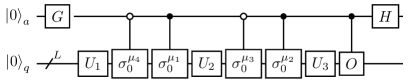
In all other cases, we can find the expected value of the non-Hermitian operator with the following observation. Since we sum over all possible combinations in Eq. (29) and the Pauli matrices are self-adjoint, the sum is going to contain the Hermitian conjugate of each summand. Hence, we do not need to determine the individual summands; it is sufficient to obtain from the quantum device. This can be done with a circuit similar to that used for the Hadamard test [47, 48]. The corresponding quantum circuit requires the addition of an ancilla qubit, which is entangled with the qubits encoding the state wave function, as shown in Fig. 3. A subsequent measurement of the expectation value of the Pauli operator yields the desired quantity. The normalization factor can be computed in a similar manner by simply setting observable .
We now specialize our investigation on the case of free staggered fermions, corresponding to in Eq. (2). The resulting ground state is trivial in momentum space and is simply given by the state with no (anti)fermionic excitations; see Eq. (49) in Appendix B for details. Hence, annihilating a (anti)fermion in this state is not possible, and acting with the operators , on the vacuum state will result in zero. This allows us to rewrite the initial state as,
| (30) |
where in the third line we have substituted in Eq. (22) with . Notice that in the last line of Eq. (30) all operators acting on the ground state are unitary. Since the time evolution operator is unitary as well, expectation values of observables in the time evolved state can simply be measured on a quantum device in a standard manner.
The simplification of the circuit discussed above applies only to the case of the free theory in case the initial state corresponds to a wave packet of one fermion and one antifermion. For more general settings considering wave packets for two or more fermions and antifermions, or when dealing with the interacting theory with a nontrivial ground state, the Hadamard test remains the only viable alternative for determining expectation values.
IV Results
In the following, we demonstrate the methods discussed above for the lattice Thirring model discussed in Sec. II and whose Hamiltonian is given in Eq. (5). We will examine two regimes: first we focus on the case of , for which the Hamiltonian corresponds to a staggered discretization of free Dirac fermions and is exactly solvable. Second, we investigate the interacting theory for , a regime where the solution of the model can no longer be obtained with analytical techniques. Lastly, we demonstrate the feasibility of our approach on current quantum hardware by simulating the evolution of the noninteracting case on IBM’s quantum devices. In both cases, we will consider initial states corresponding to the ground state with one fermion and one antifermion wave packet with opposite momenta imposed on top. Subsequently, we evolve those in time to observe the scattering of the two wave packets.
For the continuum Thirring model, the spectrum and the -matrix can be computed analytically [49, 50, 51]; see Refs. [52, 53] for slightly different interpretation.
The continuum Thirring model is equivalent to the quantum sine-Gordon model in the sector of zero topological charge [54, 55]. Due to the infinite number of conservation laws in the sine-Gordon model, there can be no particle production during the scattering process. In combination with momentum conservation, this implies that the particles can thus only exchange momentum during the scattering process [56, 57]. As such, we will restrict our discussion to the sector with constant particle number which, after the Jordan-Wigner transformation, corresponds to .
To characterize the scattering process, we calculate several observables at each time step of the evolution. First, we will measure the site-resolved particle density , which in spin language is simply given by . In order to highlight the effect of wave packets compared to the ground state of the theory itself, we subtract the particle density of the ground state and consider the quantity
| (31) |
Second, we calculate at each step of the evolution the von Neumann entropy obtained for the reduced density operator describing the subsystem of the first qubits. This quantity provides a measure for entanglement between two subsystem and . To again highlight the effect caused by the addition of the wave packets, we subtract the entropy of the ground state and consider,
| (32) |
In addition, to quantify the effect of the interaction of the wave packets, we consider the difference in von Neumann entropy obtained for a system with two wave packets compared to the sum of the entropy from two separate systems, each having either particle or an antiparticle but not both. The latter can be obtained by considering the initial states and with the same momenta and width of the wave packet as for the combined case and evolving those in time. The difference in entropy is then given by
| (33) |
where is the entropy for the time evolved state , according to Eq. (32).
IV.1 Vanishing coupling: the free fermionic case
Let us first consider the case of free staggered Dirac fermions. While the dynamics of the system in this regime can be simulated efficiently in momentum space using free fermionic techniques (see Appendix B), we choose to work in position space to benchmark the techniques developed earlier.
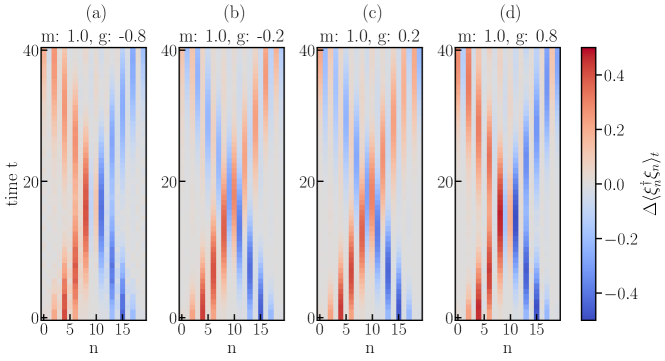
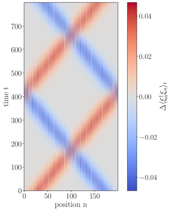
In order to demonstrate that the operators in Eq. (22) successfully create a wave packet, we first simulate the evolution in time exactly. To this end, we obtain the ground state of the Hamiltonian using exact diagonalization and subsequently compute the system’s evolution via Eq. (23) by approximating the time evolution operator via a Taylor expansion up to second order, . Here we use a time step of which is determined to be small enough to avoid noticeable numerical errors for the time scales we simulate. This allows us to easily reach a system size of 20 qubits, the results for which for the site resolved particle density throughout the evolution for various masses are shown in Fig. 4.
The particle density clearly shows the presence of the two wave packets where the fermion (antifermion) manifests itself in an excess (lack) of particle density compared to the ground state. Moreover, we see the desired effect that the wave packets are moving towards each other, where the dynamics progress faster for smaller values of the mass, as expected. Since the fermions are noninteracting, the wave packets simply pass through each other before approaching one boundary and returning on the opposite due to periodic boundary conditions.
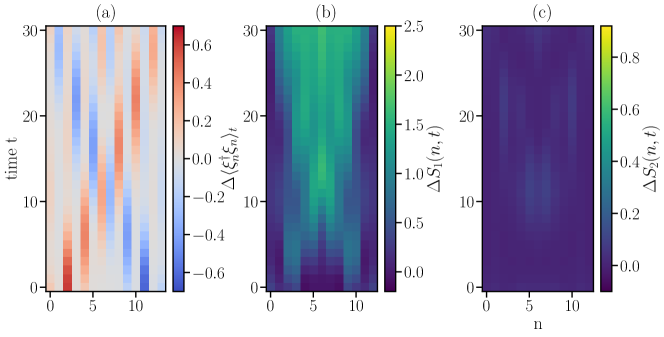
In order to gain more insight into the scattering process, we also consider the von Neumann entropy. Since computing the entropy in our direct approach requires constructing the reduced density operator, which in general is a dense matrix, we use a slightly smaller system size for computational convenience. Moreover, we do not perform a direct simulation of the state vector as in the previously, but we simulate the the circuit allowing us to compute the evolution exactly as discussed in Sec. III.3 and outlined in detail in Appendix C. For these simulations, we use Qiskit [58] assuming an ideal quantum computer without shot noise. The results for the subtracted particle density and the von Neumann entropy are shown in Fig. 5. Despite the reduced system size, the particle density reveals that we initially still have two clearly separated wave packets which propagate towards each other during the evolution and eventually pass through one other. Inspection of the site-resolved entropy, , in Fig. 5(b), there is no entanglement between the wave packets at the beginning of the evolution but as they approach one another, they become also become entangled. However, looking at the subtracted von Neumann entropy, , in Fig. 5(b) which corresponds to subtracting the sum of the entropies obtained from evolving the fermion and the antifermion wave packet individually, we see that this quantity is close to zero throughout the entire evolution. This demonstrates that there is essentially no excess entropy produced compared to evolving each wave packet individually, as expected for two noninteracting the wave packets.
IV.2 Nonvanishing coupling: the interacting case
Our approach can also be applied to the interacting case, and here we study the dynamics of the lattice Thirring model with nonvanishing coupling, . To show that the operators in Eq. (22) indeed create a wave packet corresponding to a particle-antiparticle pair to a good approximation, we first perform a direct evolution using a Taylor expansion up to second order as for the noninteracting case. The results for a system with sites and time step for various values of the coupling are shown in Fig. 6. Again, we have again checked that the step size is small enough to prevent any significant numerical errors.
For we clearly see two wave packets corresponding to a particle and an antiparticle, again appearing respectively as an excess and a deficiency in particle density compared to the ground state; c.f. Fig. 6(a). Moreover, as time progresses, we observe the wave packets are moving towards each other before eventually colliding and interacting. For small absolute values of the coupling , we observe a similar behavior as in the free case: the wave packets essentially pass through each other, as shown in Figs. 6(b) and 6(c). Comparing this to the noninteracting case (shown in Fig. 4(c)), the wave packets disperse slightly stronger for a nonvanishing coupling of , and the particle density spreading at is more pronounced. At larger absolute values of the coupling, , we observe a noticeable change in behavior. The wave packets are no longer passing though each other, but instead repel each other, as can be seen in Figs. 6(a) and 6(d).
Our observations from the direct simulation are in agreement with the theoretical prediction for the continuum model, with no observed particle production during the scattering process. Due to momentum conservation, the wave packets representing the (anti)particles either pass through each other or repel each other, depending on the coupling, . While the former behavior is observed for couplings close to zero, the latter happens if the absolute value of is close to 1.
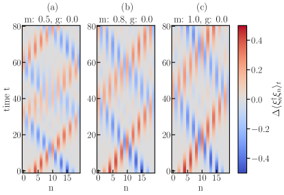
Again, we also examine the von Neumann entropy a slightly smaller system size , where we use state vector simulation in Qiskit [58] to get the vectors corresponding to the four unitary summands of Eq. (24) and get the quantum state through their combination, and we normalize the state before calculating the von Neumann entropy. For the time evolution operator, we use the matrix representation of in our simulation and the resource estimation of Trotter decomposition is left for further work. The results for various values of the coupling are depicted in Fig. 7.
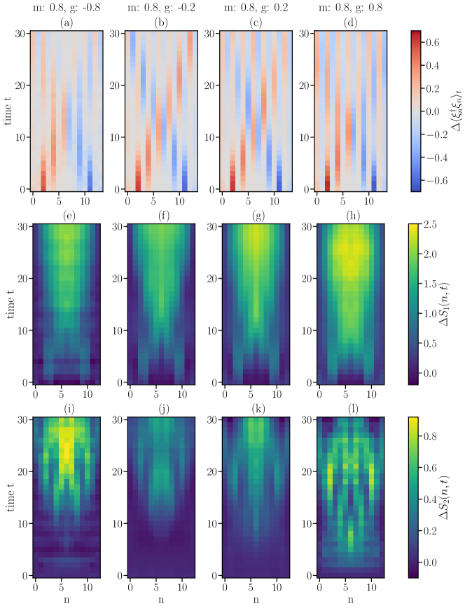
Despite the reduced system size, the particle density in panels (a) - (d) clearly shows the same effect as for : for values of the coupling close to zero the wave packets simply pass through each other, whereas for they repel each other. Focusing on the entropy in Fig. 7(e) - 7(h), we see that there is a noticeable amount of excess entropy compared to the ground state. In particular, then entropy is growing with , where for positive values of the coupling, we generally observe larger values of than for the corresponding negative value as a comparison between Figs. 7(e) and 7(h) as well as 7(f) and 7(g) reveals. While the values for the excess entropy compared to the noninteracting case are larger, the evolution of looks qualitatively similar to the noninteracting case, as a comparison with Fig. 5(h) shows.
Turning towards in Figs. 7(i) - 7(l), we now observe a clear difference between the non-interacting case and . While the non-interacting case essentially shows a homogeneous value of throughout the entire evolution, for we see a noticeable increase of at the point where the two wave packets collide with each other. Considering the same absolute value for the coupling, we generally observe that grows faster for the positive choice of than for the negative value. This is in agreement with observation in the particle density, that for a fixed value of , the collision happens at earlier times for a positive value than for the corresponding negative value (compare, e.g., Figs. 7(a) and 7(d)). Interestingly, for the time scales we study, the data for for shows a qualitatively different behavior than for . For the positive value, we see a peak in in the center of the system around when the wave packets first start to collide. This peak subsequently decays before two peaks at close to the boundary of the system emerge around , at which time the wave packets start to interact again due to the periodic boundary conditions. In contrast, for we observe a considerable increase in between the wave packets after colliding, and there is no substantial decay during the entire time we simulate.
In summary, our numerical results demonstrate that the operators we derived allow for creating wave packets corresponding to a fermion and an antifermion with opposite momenta even in the interacting regime. The (anti)particle wave packets move towards each other and start interacting, which is reflected in .
IV.3 The free fermionic case on quantum hardware
Finally, we demonstrate that our approach is feasible on current quantum hardware, and implement the noninteracting case on IBM’s quantum devices. To this end, we use a simple parametric circuit for preparing the ground state of the model with high fidelity, where the parameters have been optimized using a classical simulation222Note that finding the optimal parameters could be done with a standard VQE approach. Since our primary focus in this work lies on the time evolution, we use a classical simulation to save time on the hardware.. Subsequently, we evolve the initial state with two wave packets using the techniques for the free fermionic case, , discussed in Sec. III.3. This allows us to simulate the evolution for arbitrary times at a constant circuit depth. In order to mitigate the effects of hardware noise, we employed probabilistic error amplification (PEA) [59] with zero-noise extrapolation limit [60, 45]. For PEA, we applied Pauli twirling to each unique layer in our nominal circuit. We then generated 300 circuit instances at gain factors and sampled each of the resulting 900 circuits 1024 times to determine the average value of each observable of interest. Finally, we used an exponential fit of the averages of the measured values at different to obtain an estimate of their zero-noise value.
Figure 8 shows results for the particle density obtained on ibm_peekskill for 12 qubits in comparison with the exact results for several time steps.
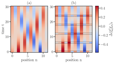
Comparing panels 8(a) and 8(b), we observe good agreement between the data from the quantum hardware and the exact solution. In particular, focusing on the time slices obtained from the quantum device in Fig. 8(b), we clearly see the two wave packets moving towards each other (, 6), before they eventually passing through () and start to move away from each other again (, 24).
To get a more detailed picture of the hardware results, we show the site-resolved data for individual time slices in Fig. 9.
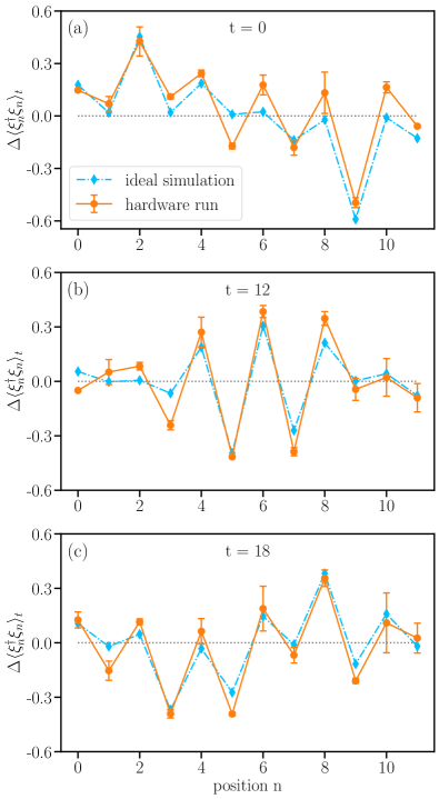
As the figure reveals, there is generally good agreement between the exact result and the experimental data from the quantum device, in most cases both results agree within error bar. In particular, the time-slices for the particle density illustrate once more the presence of two separated wave packets, showing up as a peak in the particle density around site and a dip at site for (c.f. Fig. 9(a)). These are moving towards the center as time progresses resulting in a particle density noticeably different from zero in the center of the system, as shown in Fig. 9(b). Eventually, after the two wave packets pass through each other, we observe again a well separated peak and a dip in the particle density around in Fig. 9(c).
V Conclusion and outlook
In this work, we proposed a framework for studying fermion scattering on digital quantum computing. Using the lattice Thirring model as an example, we demonstrated our framework by simulating the elastic collision for fermion-antifermion wave packets both classically and on quantum hardware.
Guided by the free theory, corresponding to the Thirring model at vanishing coupling, we derived a set of operators that allow us to create approximate fermion and antifermion wave packets for the interacting theory on top of the ground state. Starting from such an initial state, we showed how to efficiently obtain the expected value of observables from a quantum device throughout the evolution and provided the necessary quantum circuits to measure them.
To demonstrate our approach, we first simulated the dynamics of the a fermion-antifermion wave packet in the free theory exactly before proceeding to the interacting case. Observing the particle density and the von Neumann entropy produced throughout the elastic scattering, we characterized the process and showed that our framework provides an avenue towards simulating these dynamics on quantum devices. While the entropy can in general not be obtained efficiently on a quantum device, the particle density can be readily measured on a digital quantum computer. Moreover, we carried out a proof-of-principle demonstration simulating the scattering a fermion and an antifermion wave packet for the free theory on IBM’s quantum devices. Using state-of-the-art error mitigation methods, the data obtained from the quantum device is in good agreement with the theoretical prediction, thus showing that our approach is suitable for near-term quantum hardware.
Our work can be generalized to arbitrary fermionic models, and provides a first step towards simulating fermionic scattering processes on quantum computers. While we provided a demonstration on quantum hardware, a systematic study of the effects of the quantum noise is left for future work. Furthermore, our data for the particle density can serve as a benchmark for future experiments studying scattering processes in the Thirring model on a quantum device.
Acknowledgements.
IBM, the IBM logo, and ibm.com are trademarks of International Business Machines Corp., registered in many jurisdictions worldwide. Other product and service names might be trademarks of IBM or other companies. The current list of IBM trademarks is available at https://www.ibm.com/legal/copytrade. S.K. acknowledges financial support from the Cyprus Research and Innovation Foundation under the project “Quantum Computing for Lattice Gauge Theories (QC4LGT)”, contract no. EXCELLENCE/0421/0019. A. C. is supported in part by the Helmholtz Association —“Innopool Project Variational Quantum Computer Simulations (VQCS).” This work is funded by the European Union’s Horizon Europe Framework Programme (HORIZON) under the ERA Chair scheme with grant agreement no. 101087126. This work is supported with funds from the Ministry of Science, Research and Culture of the State of Brandenburg within the Centre for Quantum Technologies and Applications (CQTA).![[Uncaptioned image]](/html/2312.02272/assets/x10.jpg)
References
- et al. [2012a] G. A. et al., Observation of a new particle in the search for the standard model higgs boson with the atlas detector at the lhc, Phys. Lett. B 716, 1 (2012a).
- et al. [2012b] S. C. et al., Observation of a new boson at a mass of 125 gev with the cms experiment at the lhc, Phys. Lett. B 716, 30 (2012b).
- Dürr et al. [2008] S. Dürr, Z. Fodor, J. Frison, C. Hoelbling, R. Hoffmann, S. D. Katz, S. Krieg, T. Kurth, L. Lellouch, T. Lippert, K. K. Szabo, and G. Vulvert, Ab initio determination of light hadron masses, Science 322, 1224 (2008).
- Alexandrou [2014] C. Alexandrou, Hadron properties from lattice QCD, Journal of Physics: Conference Series 562, 012007 (2014).
- Hebenstreit et al. [2013a] F. Hebenstreit, J. Berges, and D. Gelfand, Simulating fermion production in dimensional qed, Phys. Rev. D 87, 105006 (2013a).
- Hebenstreit et al. [2013b] F. Hebenstreit, J. Berges, and D. Gelfand, Real-time dynamics of string breaking, Phys. Rev. Lett. 111, 201601 (2013b).
- Bañuls and Cichy [2020] M. C. Bañuls and K. Cichy, Review on novel methods for lattice gauge theories, Rep. Prog. Phys. 83, 024401 (2020).
- Bañuls et al. [2020] M. C. Bañuls, R. Blatt, J. Catani, A. Celi, J. I. Cirac, M. Dalmonte, L. Fallani, K. Jansen, M. Lewenstein, S. Montangero, C. A. Muschik, B. Reznik, E. Rico, L. Tagliacozzo, K. V. Acoleyen, F. Verstraete, U. J. Wiese, M. Wingate, J. Zakrzewski, and P. Zoller, Simulating lattice gauge theories within quantum technologies, Eur. Phys. J. D 74, 165 (2020).
- Bañuls et al. [2019] M. C. Bañuls, K. Cichy, J. I. Cirac, K. Jansen, and S. Kühn, Tensor networks and their use for lattice gauge theories, PoS(LATTICE 2018)022 , (2019).
- Orús [2014] R. Orús, A practical introduction to tensor networks: Matrix product states and projected entangled pair states, Ann. Phys. 349, 117 (2014).
- Bridgeman and Chubb [2017] J. C. Bridgeman and C. T. Chubb, Hand-waving and interpretive dance: an introductory course on tensor networks, J. Phys. A: Math. Theor. 50, 223001 (2017).
- Bañuls [2023] M. C. Bañuls, Tensor network algorithms: A route map, Annual Review of Condensed Matter Physics 14, 173 (2023).
- Buyens et al. [2017] B. Buyens, J. Haegeman, F. Hebenstreit, F. Verstraete, and K. Van Acoleyen, Real-time simulation of the schwinger effect with matrix product states, Phys. Rev. D 96, 114501 (2017).
- Kühn et al. [2015] S. Kühn, E. Zohar, J. Cirac, and M. C. Bañuls, Non-abelian string breaking phenomena with matrix product states, J. High Energy Phys. 2015 (7), 130.
- Rigobello et al. [2021] M. Rigobello, S. Notarnicola, G. Magnifico, and S. Montangero, Entanglement generation in qed scattering processes, Phys. Rev. D 104, 114501 (2021).
- Felser et al. [2020] T. Felser, P. Silvi, M. Collura, and S. Montangero, Two-Dimensional Quantum-Link Lattice Quantum Electrodynamics at Finite Density, Phys. Rev. X 10, 041040 (2020).
- Magnifico et al. [2021] G. Magnifico, T. Felser, P. Silvi, and S. Montangero, Lattice quantum electrodynamics in (3+1)-dimensions at finite density with tensor networks, Nat. Commun. 12, 3600 (2021).
- Calabrese and Cardy [2005] P. Calabrese and J. Cardy, Evolution of entanglement entropy in one-dimensional systems, J. Stat. Mech. 2005, P04010 (2005).
- Schuch et al. [2008] N. Schuch, M. M. Wolf, F. Verstraete, and J. I. Cirac, Entropy scaling and simulability by matrix product states, Phys. Rev. Lett. 100, 030504 (2008).
- Schachenmayer et al. [2013] J. Schachenmayer, B. P. Lanyon, C. F. Roos, and A. J. Daley, Entanglement growth in quench dynamics with variable range interactions, Phys. Rev. X 3, 031015 (2013).
- Bañuls et al. [2009] M. C. Bañuls, M. B. Hastings, F. Verstraete, and J. I. Cirac, Matrix product states for dynamical simulation of infinite chains, Phys. Rev. Lett. 102, 240603 (2009).
- Trotzky et al. [2012] S. Trotzky, Y.-A. Chen, A. Flesch, I. P. McCulloch, U. Schollwöck, J. Eisert, and I. Bloch, Probing the relaxation towards equilibrium in an isolated strongly correlated one-dimensional bose gas, Nat. Phys. 8, 325 (2012).
- Martinez et al. [2016] E. A. Martinez, C. A. Muschik, P. Schindler, D. Nigg, A. Erhard, M. Heyl, P. Hauke, M. Dalmonte, T. Monz, P. Zoller, and R. Blatt, Real-time dynamics of lattice gauge theories with a few-qubit quantum computer, Nature 534, 516 (2016).
- Klco et al. [2018] N. Klco, E. F. Dumitrescu, A. J. McCaskey, T. D. Morris, R. C. Pooser, M. Sanz, E. Solano, P. Lougovski, and M. J. Savage, Quantum-classical computation of schwinger model dynamics using quantum computers, Phys. Rev. A 98, 032331 (2018).
- Atas et al. [2023] Y. Y. Atas, J. F. Haase, J. Zhang, V. Wei, S. M.-L. Pfaendler, R. Lewis, and C. A. Muschik, Simulating one-dimensional quantum chromodynamics on a quantum computer: Real-time evolutions of tetra- and pentaquarks, Phys. Rev. Res. 5, 033184 (2023).
- Thirring [1958] W. E. Thirring, A soluble relativistic field theory, Annals of Physics 3, 91 (1958).
- Wecker et al. [2015] D. Wecker, M. B. Hastings, N. Wiebe, B. K. Clark, C. Nayak, and M. Troyer, Solving strongly correlated electron models on a quantum computer, Phys. Rev. A 92, 062318 (2015).
- Kivlichan et al. [2018] I. D. Kivlichan, J. McClean, N. Wiebe, C. Gidney, A. Aspuru-Guzik, G. K.-L. Chan, and R. Babbush, Quantum simulation of electronic structure with linear depth and connectivity, Phys. Rev. Lett. 120, 110501 (2018).
- Jiang et al. [2018] Z. Jiang, K. J. Sung, K. Kechedzhi, V. N. Smelyanskiy, and S. Boixo, Quantum algorithms to simulate many-body physics of correlated fermions, Phys. Rev. Appl. 9, 044036 (2018).
- Peruzzo et al. [2014a] A. Peruzzo, J. McClean, P. Shadbolt, M.-H. Yung, X.-Q. Zhou, P. J. Love, A. Aspuru-Guzik, and J. L. O’Brien, A variational eigenvalue solver on a photonic quantum processor, Nat. Commun. 5, 1 (2014a).
- Bañuls et al. [2019] M. C. Bañuls, K. Cichy, Y.-J. Kao, C.-J. D. Lin, Y.-P. Lin, and D. T.-L. Tan, Phase structure of the ()-dimensional massive thirring model from matrix product states, Phys. Rev. D 100, 094504 (2019).
- Coleman [1975] S. Coleman, Quantum sine-gordon equation as the massive thirring model, Phys. Rev. D 11, 2088 (1975).
- Kogut and Susskind [1975] J. Kogut and L. Susskind, Hamiltonian formulation of wilson’s lattice gauge theories, Phys. Rev. D 11, 395 (1975).
- Susskind [1977] L. Susskind, Lattice fermions, Phys. Rev. D 16, 3031 (1977).
- Lieb et al. [1961] E. Lieb, T. Schultz, and D. Mattis, Two soluble models of an antiferromagnetic chain, Ann. Phys. 16, 407 (1961).
- Verstraete et al. [2009] F. Verstraete, J. I. Cirac, and J. I. Latorre, Quantum circuits for strongly correlated quantum systems, Physical Review A 79, 032316 (2009).
- Zohar et al. [2016] E. Zohar, J. I. Cirac, and B. Reznik, Quantum simulations of lattice gauge theories using ultracold atoms in optical lattices, Rep. Prog. Phys. 79, 014401 (2016).
- Jordan and Wigner [1993] P. Jordan and E. P. Wigner, Über das paulische äquivalenzverbot (Springer, 1993).
- Belyansky et al. [2023] R. Belyansky, S. Whitsitt, N. Mueller, A. Fahimniya, E. R. Bennewitz, Z. Davoudi, and A. V. Gorshkov, High-energy collision of quarks and hadrons in the schwinger model: From tensor networks to circuit qed, arXiv:2307.02522 (2023).
- Peruzzo et al. [2014b] A. Peruzzo, J. McClean, P. Shadbolt, M.-H. Yung, X.-Q. Zhou, P. J. Love, A. Aspuru-Guzik, and J. L. O’Brien, A variational eigenvalue solver on a photonic quantum processor, Nat. Commun. 5, 1 (2014b).
- McArdle et al. [2019] S. McArdle, T. Jones, S. Endo, Y. Li, S. C. Benjamin, and X. Yuan, Variational ansatz-based quantum simulation of imaginary time evolution, npj Quantum Information 5, (2019).
- Gacon et al. [2023] J. Gacon, J. Nys, R. Rossi, S. Woerner, and G. Carleo, Variational quantum time evolution without the quantum geometric tensor, arXiv:2303.12839 (2023).
- Nielsen et al. [2002] M. A. Nielsen, M. J. Bremner, J. L. Dodd, A. M. Childs, and C. M. Dawson, Universal simulation of hamiltonian dynamics for quantum systems with finite-dimensional state spaces, Phys. Rev. A 66, 022317 (2002).
- Miessen et al. [2023] A. Miessen, P. J. Ollitrault, F. Tacchino, and I. Tavernelli, Quantum algorithms for quantum dynamics, Nature Computational Science 3, 25 (2023).
- Li and Benjamin [2017] Y. Li and S. C. Benjamin, Efficient variational quantum simulator incorporating active error minimization, Phys. Rev. X 7, 021050 (2017).
- Barison et al. [2021] S. Barison, F. Vicentini, and G. Carleo, An efficient quantum algorithm for the time evolution of parameterized circuits, Quantum 5, 512 (2021).
- Chiesa et al. [2019] A. Chiesa, F. Tacchino, M. Grossi, P. Santini, I. Tavernelli, D. Gerace, and S. Carretta, Quantum hardware simulating four-dimensional inelastic neutron scattering, Nature Physics 15, 455 (2019).
- Endo et al. [2020] S. Endo, I. Kurata, and Y. O. Nakagawa, Calculation of the green’s function on near-term quantum computers, Phys. Rev. Res. 2, 033281 (2020).
- Luther [1976a] A. Luther, Eigenvalue spectrum of interacting massive fermions in one dimension, Phys. Rev. B 14, 2153 (1976a).
- Korepin [1979] V. E. Korepin, DIRECT CALCULATION OF THE S MATRIX IN THE MASSIVE THIRRING MODEL, Theor. Math. Phys. 41, 953 (1979).
- Korepin [1980] V. E. Korepin, The mass spectrum and the S matrix of the massive Thirring model in the repulsive case, Communications in Mathematical Physics 76, 165 (1980).
- Luther [1976b] A. Luther, Eigenvalue spectrum of interacting massive fermions in one dimension, Phys. Rev. B 14, 2153 (1976b).
- Luscher [1976] M. Luscher, Dynamical Charges in the Quantized, Renormalized Massive Thirring Model, Nucl. Phys. B 117, 475 (1976).
- Coleman [1976] S. Coleman, More about the massive schwinger model, Ann. Phys. (N.Y.) 101, 239 (1976).
- Mandelstam [1975] S. Mandelstam, Soliton operators for the quantized sine-gordon equation, Phys. Rev. D 11, 3026 (1975).
- Zamolodchikov [1977] A. B. Zamolodchikov, Exact Two Particle s Matrix of Quantum Sine-Gordon Solitons, Pisma Zh. Eksp. Teor. Fiz. 25, 499 (1977).
- Karowski and Thun [1977] M. Karowski and H. J. Thun, Complete S Matrix of the Massive Thirring Model, Nucl. Phys. B 130, 295 (1977).
- Qiskit contributors [2023] Qiskit contributors, Qiskit: An open-source framework for quantum computing (2023).
- Kim et al. [2023] Y. Kim, A. Eddins, S. Anand, K. X. Wei, E. van den Berg, S. Rosenblatt, H. Nayfeh, Y. Wu, M. Zaletel, K. Temme, and A. Kandala, Evidence for the utility of quantum computing before fault tolerance, Nature 618, 500 (2023).
- Temme et al. [2017] K. Temme, S. Bravyi, and J. M. Gambetta, Error mitigation for short-depth quantum circuits, Phys. Rev. Lett. 119, 180509 (2017).
Appendix A Details of Givens rotation
In this section, we explain how to decompose a complex unitary matrix based on Givens rotation. We then demonstrate how to decompose the operation into local operations based on this decomposition of .
Given a complex unitary matrix with dimensions , we can find a series unitary matrices and that diagonalize the matrix as follows
| (34) |
where
| (36) | |||
| (37) |
The matrix is serves to diagonalize the -th column of matrix . In this process, the diagonal matrix eliminates the phase of elements in column and then Givens rotation matrix eliminates the element . The formula of matrix and are as following:
| (38) |
| (39) |
where the matrix is diagonal except for -th, -th row and columns.
Below, we illustrate the procedure for the diagonalization of the first column of . Considering a general complex unitary matrix :
| (40) |
where , are the absolute value and phase of matrix element . In order to diagonalize the first column of . We will multiply the phase matrix to such that the elements in first column of become real. The parameters in are denoted as , and the matrix is as follows:
| (41) |
In the above, the phase of the first column in is eliminated by , and the phase of elements in other columns are changed to . Subsequently, we can utilize the matrix to induce a rotation between the -th row and -th row. With a rotation angle , the rotation is able to zero the element :
| (42) | ||||
In the resulting matrix above, all the matrix elements in -th row and -th row are changed due to the Givens rotation. To simplify, we use and to represent the absolute value and phase of matrix elements after the rotation. To diagonalize the first column of the matrix , we need to multiply more Givens rotation matrix to to zero the matrix elements on the row in first column:
| (43) | ||||
where for . Furthermore, the first elements of other columns are also zeros after diagonalizing the first column. This occurs due to the orthogonality between different columns in a unitary matrix. The procedure is similar if we want to diagonal the second column of , and so on… In the wave packet preparation, we specifically focus on the first column of , denoted by . Therefore, assuming , the decomposition of u will be:
| (44) |
Regarding the unitary operator defined in Eq. (16), one can get a decomposition of it based on the property and the decomposition of matrix :
| (45) |
with,
| (46) | ||||
The final equation above employs the following result, which is non-zero only for the elements with indices and :
| (47) |
Appendix B Momentum space and Fock space
In this appendix, we analytically determine the particle density noninteracting case during the scattering process via calculations in momentum and Fock space. Since we are dealing with a free fermionic system, these computations involve a matrices whose dimensions , enabling us to numerically simulate the phenomenon for large system and to cross-check the results in position space.
In momentum space, the free fermion Hamiltonian is diagonal in terms of the fermionic and antifermionic creation (annihilation) operators , (, [15]:
| (48) |
and the vacuum in this theory is the state with no excitations of fermions and antifermions:
| (49) |
As there is no interaction between fermions and antifermions in momentum space, the wave function of the system is as the tensor product of the wave function for fermion and antifermion subsystems:
| (50) |
When considering the Fock basis for the momentum state, the Gaussian wave packets for the fermion and antifermion can be represented as the vectors
| (51) | ||||
| (52) |
with . In this basis, the fermion and antifermion part of Hamiltonian correspond to diagonal matrices with dimension and the full Hamiltonian will be a direct sum of the matrix for the fermions and the antifermions. The fermionic part will be given by
| (53) |
and analogously the antifermionic part. As a result, the time evolution of the initial fermionic Gaussian wave packet can be expressed as follows (up to a global phase)
| (54) | ||||
| (55) |
To obtain the particle density, at each spatial site, we need to transform the operator into momentum space. For even we find
| (56) |
For odd , we obtain
| (57) |
where the constant and are the particle density of the vacuum for even and odd sites. The definition of and can be found in Eq. (10). Using the matrix representation in one-particle Fock space , we can evaluate the particle density quickly by calculating . We show the result with 200 sites in Fig. 10.
Appendix C Decomposition of the time evolution operator in noninteracting case
In the noninteracting case, corresponding to in Eq. (2), the Hamiltonian is quadratic in the fermionic operators and thus corresponds to a free staggered Dirac fermions. The time evolution operator operator for this case reads as
| (58) | ||||
where is an antihermitian matrix in Fock space depending only on the mass and evolution time
| (59) |
As Eq. (58) reveals, the operator has the same form as Eq. (16) with . Thus, we can use Givens rotation to decompose the time evolution operator in the same way as . Appendix A provides a comprehensive explanation of how to use Givens rotation to diagonalize the first column of the unitary matrix . The remaining columns can then successively brought to diagonal form by repeating the procedure and eventually resulting in the decomposition of . Parallelizing the Givens rotations on distinct qubit-pairs, the time evolution operator in the noninteracting case can be decomposed into a quantum circuit of constant depth , using CNOT gates.