Study of a cubic cavity resonator for gravitational waves detection in the microwave frequency range
Abstract
The direct detection of gravitational waves (GWs) of frequencies above MHz has recently received considerable attention. In this work we present a precise study of the reach of a cubic cavity resonator to GWs in the microwave range, using for the first time tools allowing to perform realistic simulations. Concretely, the BI-RME 3D method, which allows to obtain not only the detected power but also the detected voltage (magnitude and phase), is used here. After analyzing three cubic cavities for different frequencies and working simultaneously with three different degenerate modes at each cavity, we conclude that the sensitivity of the experiment is strongly dependent on the polarization and incidence angle of the GW. The presented experiment can reach sensitivities up to at 100 MHz, at 1 GHz, and at 10 GHz for optimal angles and polarizations, and where in all cases we assumed an integration time of ms. These results provide a strong case for further developing the use of cavities to detect GWs. Moreover, the possibility of analyzing the detected voltage (magnitude and phase) opens a new interferometric detection scheme based on the combination of the detected signals from multiple cavities.
1 Introduction
The direct detection of gravitational waves (GWs) by Earth interferometers opened a new era in our quest to understand the constituents of the Universe [1]. These detectors have been able to explore GWs in a band around Hz [2]. Equally relevant are the recent detections by pulsar timing arrays (PTA) [3, 4, 5, 6] of GWs in the nHz band, whose origin is still to be determined. The exploration of GWs in other frequency bands is a very active and promising field of research. This is partly due to the rich variety of sources expected in basically all the band from Hz (covered by CMB observations [7]) to 10 kHz. Of particular interest for future searches are the space-based interferometers, such as LISA [8], with maximum sensitivity around Hz and an impressive scientific legacy. Ideas abound to continue exploring GWs in band from nHz to kHz, such as updated ground-based laser interferometers [9, 10, 11], atom interferometers [12, 13, 14], other space missions [15, 16], or proposals related to orbital tracking [17, 18]. As mentioned, this fantastic coverage is particularly relevant given the amount of signals expected to be present, carrying information about astrophysics as well as fundamental physics.
The extension to frequencies above 10 kHz has been less explored for different reasons. First, as the frequency grows, the devices most sensitive to these GWs of shorter wavelength become smaller and may also require faster readouts. Furthermore, and relevant for interferometers, the effect of GWs on the relative distance of test masses at distances decreases as , with being the amplitude of the wave. Finally, it is not clear which astrophysical/fundamental sources may produce GWs at kHz at levels that will impact our detectors. It has been recently emphasized that these aspects may be turned into new opportunities [19]: on one hand, smaller devices may imply a connection with the cutting-edge precision of the most sensitive sensors, and call for rethinking the possible detection strategies. On the other hand, the absence of astrophysical sources may be also positive, since any significant signal may mean a deviation from the standard model. In fact, there are known candidates for GWs at high frequencies of stochastic or coherent nature, though the expectation is that any detection by current technologies may point towards new physics [19]. Independently of these points, being at the dawn of the exploration of high frequency gravitational waves (HFGWs), it is almost unquestionable the relevance of understanding its current limits and future prospects.
Out of the possible effects that a GW may generate as it traverses a laboratory, we will focus on those related to the current generated by a GW in the presence of a background electromagnetic field, called inverse Gertsenshtein effect when the electromagnetic background field is a static magnetic field [20, 21] (see also [22, 23] for other recent proposals to detect HFGWs). As a result, any technique used to detect (low energy) photons in the presence of an electromagnetic background may, in principle, be used as a GW detector. This is the idea behind the recent proposals, such as [24, 25, 26, 23], which consider experiments conceived to detect the conversion of axions into photons in the presence of a magnetic field as GW detectors. Our goal in this paper is to perform a study of this effect with the advanced tools and language used in the simulations of radio frequency resonant cavities. This is the first step towards the more ambitious goal of fully charactirizing the optimal way to search for HFGWs in these devices and start exploring new read-out ideas before performing dedicated searches (see the recent [26] for related work in this direction).
In this work we apply a full-wave modal technique for the rigorous electromagnetic study of the coupling GWs-cavity which is based on the advanced modal technique Boundary Integral - Resonant Mode Expansion (BI-RME) 3D [27]. This method allows for an efficient characterization of the interaction between the GW and the resonant cavity. The GWs generate an external induced current which excites the resonant modes of the cavity under the presence of an intense static magnetic field. Using the BI-RME 3D formulation, we are able to represent the excited resonator in terms of an equivalent network driven by the current sourced by GWs. Finally, we will compute both the voltage and the power extracted from the cavity obtaining information about the magnitude and the phase of the detected signal. As an application, we have designed a cubic resonator with three orthogonal coaxial antennas which allow for the synchronous detection of an incident GW; both polarizations of the GWs have been accounted for.
This paper is organized as follows. After this introduction, we review the basic theory for the derivation of the current densities induced by the GWs in the presence of a stationary magnetic field in section 2. Next we introduce the BI-RME 3D theory in section 3. As an application of the presented formulation, in section 4 we design three cubic resonators tuned at MHz, GHz and GHz, obtaining sensitivities, and extracted power levels and voltages for the best sensitivities. Finally, conclusions and future research lines are presented in section 5.
2 The system GW-EM fields: induced current
As shown in [28] (see also [24, 25]), in the presence of a GW with field values , being the position vector and the time measured in the reference frame of the laboratory, the Maxwell’s equations are modified to111Recall that Greek letters run as , while Latin letters have only spatial part . We use the metric convention. In this section we will stick to the units . For the calculations in the following sections, we will convert to the SI. Two repeated indexes are always summed over.
| (2.1) |
where is the effective induced current density and
| (2.2) | ||||
where is the trace of the GW, is the Levi-Civita symbol, are the components of the electric field, and those of the magnetic field. Quite relevantly, the values of for a GW seen in the laboratory are those associated to the so-called laboratory frame, which for a GW of angular frequency propagating in the direction () read [25, 28]
| (2.3) | ||||
where , is the unitary vector in the propagation direction of the GW, and is the imaginary unit. In the previous equation represents the GW as seen in the transverse-traceless coordinate system [2],
| (2.4) |
evaluated at the origin . Finally, the vectors generating the tensor structure for the polarizations have to be orthogonal to and of unit norm. In the cases we will explore, we will assume that the wave is travelling along one of the Cartesian planes, and will be chosen as the Cartesian coordinate perpendicular to it while . From the previous expressions one can now compute the effective current for different geometries. The final form of the current is not particularly illuminating, except for simple cases, and is omitted.
3 The BI-RME 3D formulation
In the second half of the last century many research groups worldwide developed several numerical techniques for the electromagnetic analysis of microwave passive components and circuits. Some of them, such as the Finite Element Method (FEM) [29, 30], the Finite Different in Time Domain (FDTD) [31] and the Transmission Line Method (TLM) [32], have a very general range of applicability in complex geometries including the presence of dielectric and/or magnetic media, and, for these reasons constitute nowadays the basis of many commercial software [33, 34, 35]. Besides, other numerical techniques such as the Method of Moments [36] and the Mode Matching Method [32] are able to deal only with specific components. However, these techniques require intense analytical processing, and, for this reason, they are not so popular, even though the developed codes are extremely fast and accurate [37, 38].
Among the modal methods proposed in the eighties and nineties, it should be mentioned the formulation proposed by Prof. Giuseppe Conciauro and co-workers at the Università degli Studio di Pavia (Italy) called the BI-RME 3D method, which represents an advanced full-wave modal technique for the accurate and efficient electromagnetic analysis of microwave arbitrarily-shaped cavities [27, 39, 40] including metallic obstacles [41, 42]. The complete formulation and the different implementations are very extensive and can be found in the technical literature [43].
In the case of a microwave cavity resonator connected to different waveguide-ports, the starting point of the BI-RME 3D method is to express the time-harmonic (complex phasors) electric and magnetic fields generated by volumetric electric current density sources and surface magnetic current density sources within the cavity with the following integral expressions (given now in the SI system),
| (3.1) | |||||
and
| (3.2) | |||||
where is the simply connected volume of the empty resonator, which is bounded by perfectly conducting walls (conducting walls of the structure are lossless, but lossy walls will be further accounted for with the conventional perturbative method in equation (3.4)). Vacuum is characterized by the electric permittivity and the magnetic permeability of free space (dielectric and magnetic media can be accounted for in the BI-RME 3D theory, but they will not be considered in this work). In these equations is the vacuum impedance; is the free space wavenumber; is the speed of light in vacuum; is the inward unitary normal vector to the cavity surface; is the surface divergence operator [44]; and are the electric and magnetic static scalar potentials Green’s functions of the cavity in Coulomb gauge, respectively; and and are the electric and magnetic dyadic potentials Green’s functions of the cavity in Coulomb gauge, respectively. The derivation of (3.1) and (3.2), as well as the closed form and relationships of both scalar and dyadic electric and magnetic potential Green’s functions in Coulomb gauge, are cumbersome and can be found in the references cited for the BI-RME 3D theory.
From a physical point of view, we want to remark that the surface magnetic currents are a mathematical artefact to represent the physical connection of the waveguide-ports with the inner of the cavity (otherwise the electric tangential component on the perfect conducting walls vanishes). On the other hand, they could also be used to describe electromagnetic field discontinuities existing on surfaces separating different regions as reported in [23]. In this study, we assume that the magnetic field is homogeneous in a significant region containing the cavity, and ignore the surface terms associated to the jumpt to a region where it vanishes. Once a set-up with a concrete magnetic field configuration is decided, our method allows to easily include these current in the analysis222We thank Camilo García-Cely and Valerie Domcke for clarifying discussions on this point..
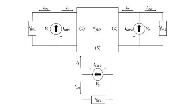
At this point we will use the parallelism existing between the detection of dark matter axions and GWs in the context of the BI-RME 3D theory. For such purpose, we will use the theory developed in [45] for the rigorous electromagnetic analysis of the dark matter axion-photon coupling existing in a microwave cavity under the presence of an intense static magnetic field . In that work, some of us detailed the successful application of the BI-RME 3D method to a time-harmonic equivalent axion electric current density , which was treated as an external source. For the GWs the formulation is similar so we will omit the mathematical derivation. Finally, the BI-RME 3D method states that the transformation of the GWs into electromagnetic energy can be formulated in terms of a set of time-harmonic current sources exciting the cavity, which is represented by its admittance matrix [46, 47] as can be seen in figure 1 for the case of ports. In this first approach, we have neglected the effect of the higher-order modes excited in the waveguide ports, considering only the fundamental mode. The expression of the current sources is given by the following formula,
| (3.3) |
for , and where refers to the resonant modes of the cavity, being the total number of the set of resonant modes considered in the summation; is the perturbed wavenumber due to the finite electric conductivity of the metallic walls [48, 46, 49] given by
| (3.4) |
being the unloaded quality factor of the -th resonant mode, and its unperturbed wavenumber. Finally, in expression (3.3), and are the normalized electric and magnetic solenoidal eigenvectors of the cavity corresponding to the eigenfactor , as reported in [45]; and represents the magnetic field of the first mode (fundamental mode) of the waveguide-port , which has to be properly normalized as described in [45]. Now, it is important to remark that the first integral of (3.3) is a surface integral performed over the access waveguide-port surface , which accounts for the coupling between the cavity and the port . Regarding the second integral, it is a volume integral performed over the entire volume of the cavity which is directly related to the coupling between the -th resonant mode and the current induced by the GW.
The BI-RME 3D formulation allows us to analyze the excitation of a microwave cavity by a GW through a full-wave modal technique, as it is shown in figure 1, where the current sources , and inject electromagnetic energy generated by the GW to both the cavity (represented by its admittance matrix) as well as to the external three ports. Evidently, the energy injected into the cavity will be dissipated by the Joule effect (Ohmic losses), whereas the energy delivered to the ports might allow for the detection of the GW. We will also demonstrate that information about the amplitude and the phase of the detected signals in all the ports can be calculated with the present technique, contrary to conventional methods based on a figure of merit, which only provides information about the power of the signal generated by the GW.
In order to proceed, we will apply the Kirchhoff laws for each waveguide-port of the figure 1, resulting in
| (3.5) |
for , where and are the wave impedance and admittance of the waveguide-port , respectively, which are related by . The classical Microwave Network Theory [46, 47] relates the voltages at the waveguide ports and the currents entering into the cavity of a microwave linear passive component (as a cavity) with the multi-port single-mode admittance matrix that for the case of ports is given by
| (3.6) |
By inserting (3.5) into (3.6) and after simple mathematical manipulations, we are able to obtain the relationship between the unknown voltages and the GW current sources ,
| (3.7) |
which is a linear system that allows one to obtain the modal voltages at the cavity ports.
Finally we can calculate the extracted power in each port as,
| (3.8) |
where ∗ denotes complex conjugate.
4 Application: design of a cubic cavity for GWs detection
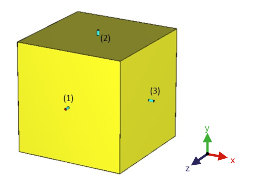
During the last years, several researchers have studied the possibility to use microwave haloscopes designed for dark matter axions detection in the search of GWs making use of already existing experimental facilities, see e.g. [24, 25, 26]. In this work we have decided to go one step further by proposing the design of a novel cavity for the detection of GWs. Since the coupling of a GW with a resonator is quite cumbersome, we propose to use a cubic cavity because it allows for the simultaneous detection of three degenerate resonant modes using three mutually perpendicular coaxial antennas, as it has been depicted in figure 2. The use of a cubic cavity may not seem ideal from the possible losses of the corners, though this can be overcome by smoothing them using rounded corners [50]. Also, the coupling of a GW to a cubic geometry may not be the most efficient one. Despite these aspects, the simplicity of the design and simulations together with the possibility of using degenerate modes overcome these caveats, and justify our choice of a cubic cavity. We leave a full optimization of the cavity design to future work. The selected set of degenerate modes are the , and , whose resonant frequencies are
where is the edge length of the cube. It is evident that, in the absence of a GW, the three degenerate modes are identical from a physical point of view due to the symmetry of the cubic resonator.
As discussed in section 2, the GWs generate a certain electromagnetic current in the presence of an external intense magnetostatic field . From (2.1), the associated volumetric electric current density can be written as
| (4.1) |
where the two components are the currents associated to the cross () and plus () polarizations present in (2.4). Once written in SI units, this suffices to describe the presence of GWs within a microwave resonator in the BI-RME 3D scenario. Here and in the following we assume that the external magnetostatic field is homogeneous and oriented in the axis of a Cartesian reference system centered in the center of mass of the cavity, .
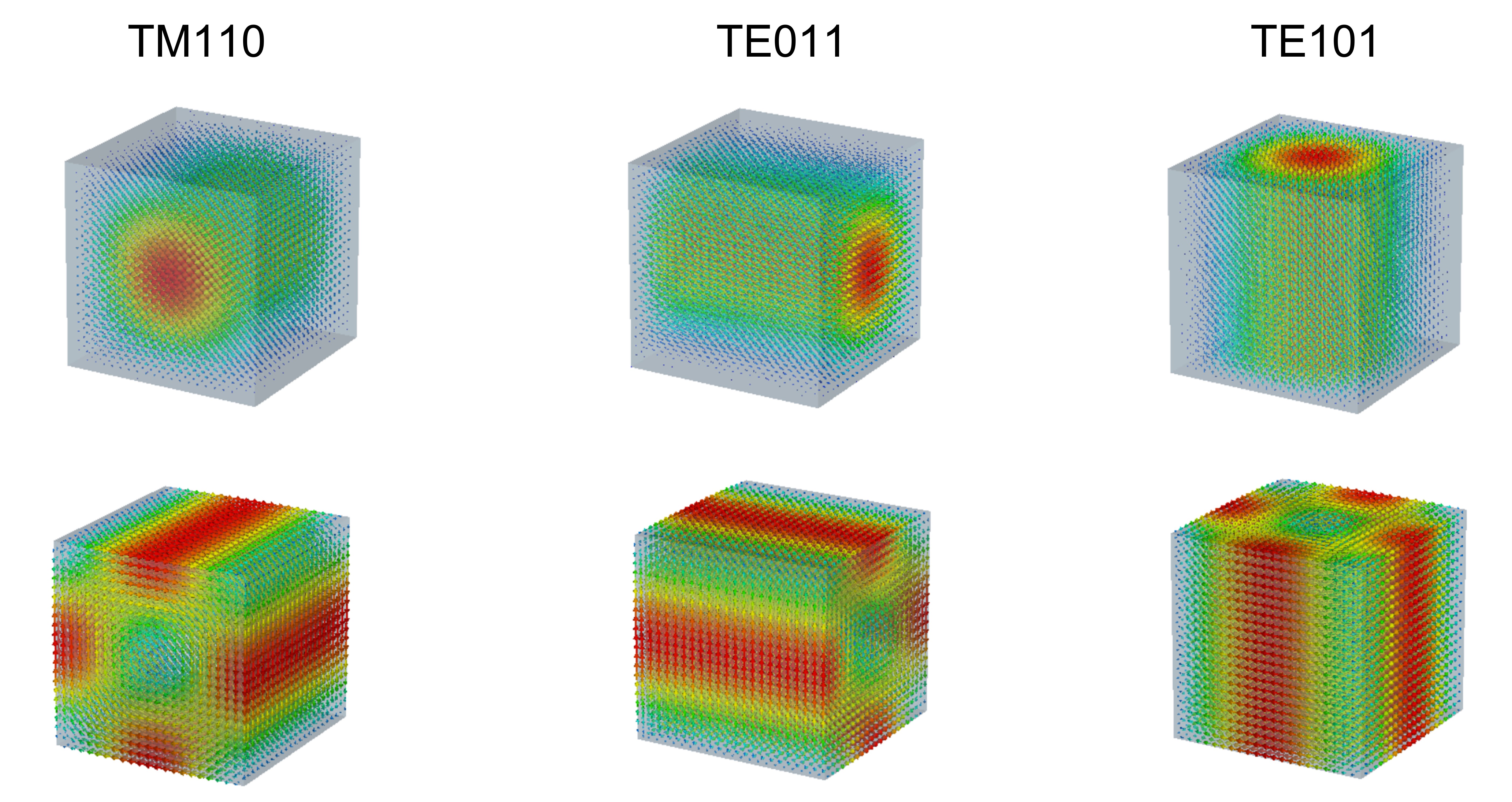
In this section we will apply the BI-RME 3D technique described in section 3 to the accurate and efficient characterization of a cubic cavity. In order to explore different ranges of frequencies, we have studied three cavities tuned at MHz (Cavity 1: C1), GHz (Cavity 2: C2) and GHz (Cavity 3: C3). Numerical simulations in this section have been made with the commercial software CST Studio [33], and post-processed with Matlab [51]. Table 1 summarizes the characteristics of the cavities. The electromagnetic field distributions of these modes have been plotted in figure 3. The unloaded quality factors of the three modes have been calculated [46] with the electric conductivity of copper at cryogenic temperature, S/m. The coaxial connectors used for the line - cavity coupling probes are BNC for C1, and SMA for C2 and C3; their inner radii , outer radii , relative dielectric permittivity and the penetration distance of the coaxial antenna inside the cavity for critical coupling regime are also reported in table 1. The reflection scattering parameters at the resonance frequencies are around dB for the three antennas of the three cavities, which indicates a good level of critical coupling regime. The characteristic coaxial impedance of the three coaxial probes of each cavity is given by
where is the characteristic coaxial admittance, and and are the wave coaxial impedance and admittance, respectively. The impedance of both BNC and SMA coaxial connectors is .
From an experimental point of view, it is important to remark that the complex voltage (phasor) measured in the coaxial waveguide ports can be easily calculated as a function of the waveguide ports voltages resulting in [45],
| CAVITY 1 | CAVITY 2 | CAVITY 3 | |
| (mm) | 2119.85 | 211.98 | 21.19 |
| (mm) | 7.00 | 0.0635 | 0.0635 |
| (mm) | 16.00 | 0.211 | 0.211 |
| 1.00 | 2.08 | 2.08 | |
| (mm) | 32.80 | 5.30 | 0.21 |
4.1 Coupling form factor
In order to analyze the coupling between the GWs and the resonant modes, we have used the definition of the dimensionless form factor between the GW and the mode introduced in [25],
| (4.4) |
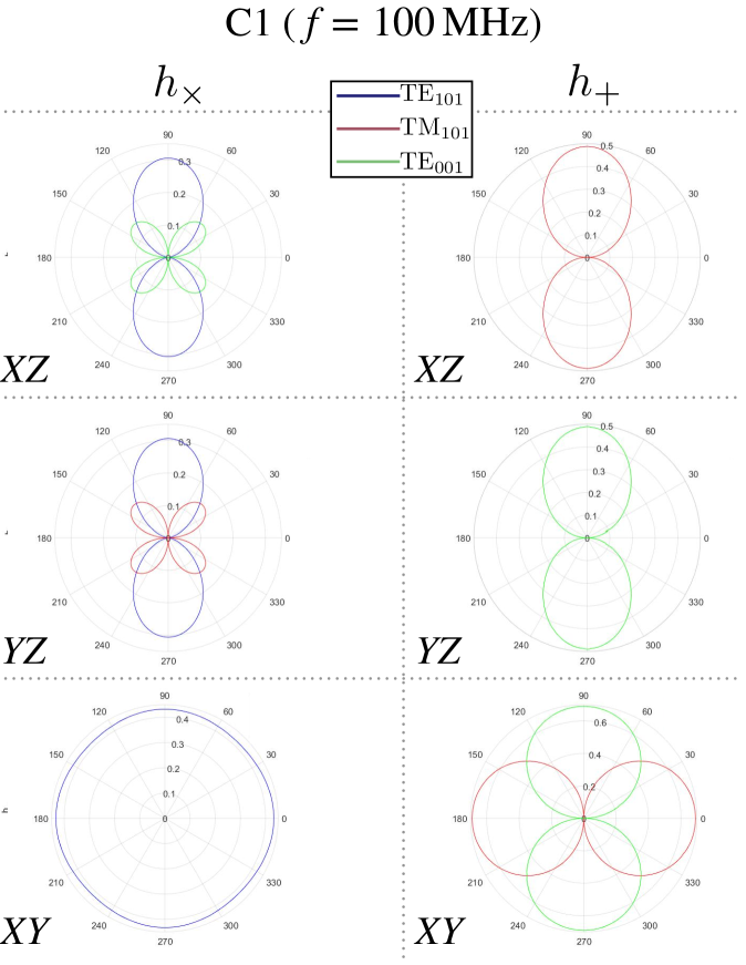
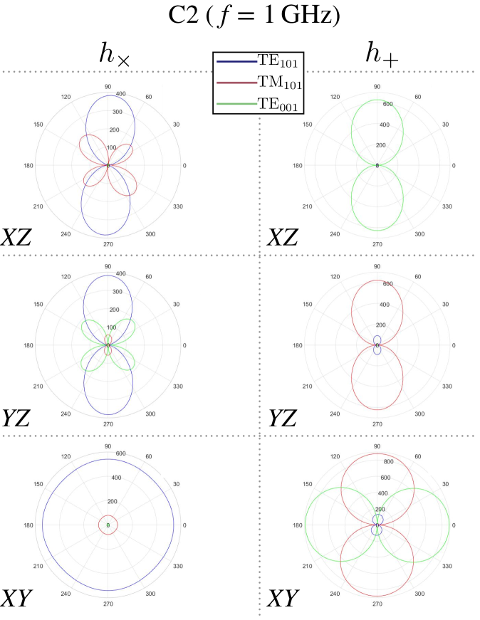
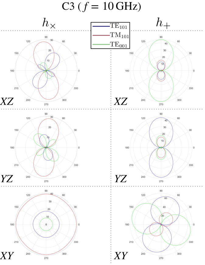
where the integral of the denominator is equal to one because of the orthonormalization condition used in BI-RME 3D [27]; is the volume of the cavity. This parameter has been represented in polar coordinates as a function of the incidence angle of the GW with respect to the axis for waves propagating along the , planes ( refers to the axis) and the angle with respect to the axis for waves propagating in the plane ( direction refers to the axis in this case). The value of is shown in terms of in figures 4, 5 and 6 for the C1, C2 and C3 cavities, respectively. As clear from these plots, the coupling strongly depends on the direction of the incidence plane, the polarization and the operation frequency.
It is important to remark here that this form factor is of very different nature than the form factor in dark matter axion detection. Whilst the latter does not depend on any axion intrinsic parameter, in the case of the graviton, the form factor depends on the complex relationship of the induced current () with frequency. This makes this factor not normalized and implies that changes with frequency are not just due to the cavity geometry, but also to the frequency dependence of the GW induced current. This explains that figures 4 - 6 show different magnitude scales.
It is also worth noting that, unlike the axion haloscope, a cavity for GW detection can work with modes whose electrical field is not aligned with the external magnetic field. This can be observed, for instance, in figure 4 for the cross polarization case, where the () gets the best form factor in most angles of incidence. This allows for more freedom in selecting resonant modes and opens up novel opportunities for the design of microwave-cavity gravitational-wave detectors.
Moreover, figures 4 - 6 also provide two crucial findings. The first one is that gravitational wave energy is transformed into currents inside the cubic cavity, which excite the three orthogonal degenerate modes. Thus, utilizing a probe for each of these degenerate modes and the right mix of the extracted signals, allow for improved detection sensitivity. Because the gravitational wave stimulates all degenerate modes at the resonant frequency, omitting to combine signals would result in a loss of sensitivity. Alternatively, we can profit from this multiple coupling of the GW by slightly detuning the three degenerate modes (for instance by proper movement of small mechanical parts in the cavity). In this way, the three modes are no longer degenerate, allowing the GW detection in three different and very close frequencies. The same applies for higher order modes, provided that their form factors are adequate for detection.
A further finding is that combining the degenerate modes in the proposed cubic cavity results in some cases in increasing the range of incident angles that can be detected (see figures 4 - 6, plane , plus polarization case). From a practical point of view, the preferred mode for detection will be that with larger values of the form factor and which shows a more isotropic behavior in order to be able to detect GWs impinging from different directions. Table 2 shows the proper modes following this criterium for the cavity C1. The best behaviour is found for GWs in the plane for the three cavities. In this case, only one mode is necessary for covering all possible angles for cross polarization. Nevertheless, the plus polarization requires a combination (sum) of two modes in order to avoid blind angles. In the other planes the combination of modes does not avoid completely blind angles. That is the case for in the and planes for both polarizations. In these cases there are different options to obtain a proper form factor for these angles, as rotating the cavity inside the magnet to modify the magnetostatic field direction with regard to the cavity coordinate system, or using a second rotated cavity, or, for long enough signals, one can profit from the rotation of the Earth to achieve this change.
| XZ plane | YZ plane | XY plane | |
|---|---|---|---|
| polarization | |||
| polarization | / |
In order to compute the detected power at each port, we have assumed that the GW impinges in the angle which generates the maximum coupling between the GW and the cavity mode, as reported in table 3.
| CAVITY 1 (C1) | CAVITY 2 (C1) | CAVITY 3 (C1) | |
|---|---|---|---|
| plane | |||
| plane | |||
| plane |
| Cavity | V (L) | Magnet | (T) | (mK) | (K) | (kHz) |
|---|---|---|---|---|---|---|
| C1 | 9526.1056 | KLASH [52] | 0.6 | 4500 | 8 | 5 |
| C2 | 9.5243 | CAPP [53] | 12 | 30 | 1 | 10 |
| C3 | 0.0095 | CAPP [53] | 12 | 30 | 1 | 20 |
4.2 Sensitivity analysis
In this first analysis of the problem we have neglected the inter-coupling effect of the three coaxial probes of each cavity, which is a good approach given that the level of the transmission scattering parameters at the resonant frequencies is around dB for the three coaxial antennas of the three cavities. As a consequence, we will neglect the mutual coupling among the three probes of each cavity, and assume that they operate independently. Thus, we do not need to solve the linear system represented in (3.7). Consequently, the power detected at each port can be expressed as
| (4.5) |
which is proportional to the GW amplitude square .
The Dicke radiometer equation [47] provides the noise power at port ,
| (4.6) |
where is the Boltzmann constant, is the noise temperature of the system at port , is the detection bandwidth, and is the detection time. This equation allows us to calculate the exclusion limits for the sensitivity of the experiment at port given and amplitude of the GW for a given signal-to-noise ratio . By inserting (4.5) and (4.6) in the definition of , we finally obtain, for each ,
| (4.7) | |||||
4.3 Realistic sensitivities and discussion
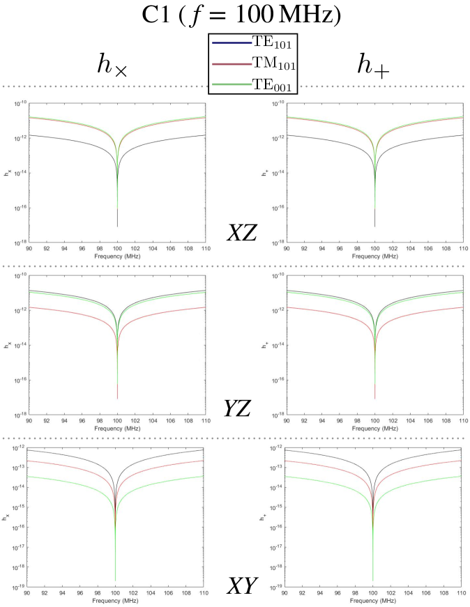
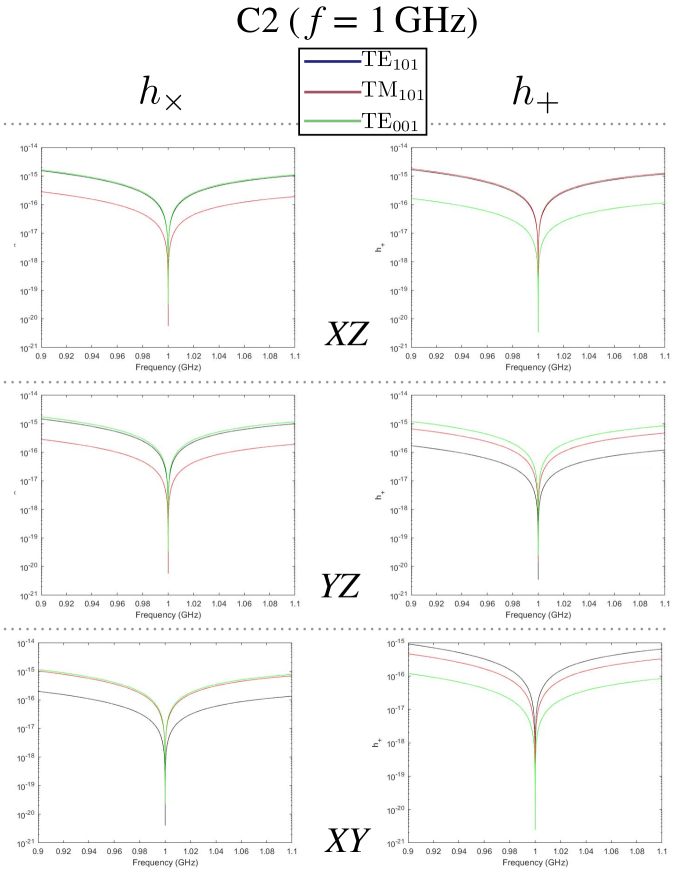
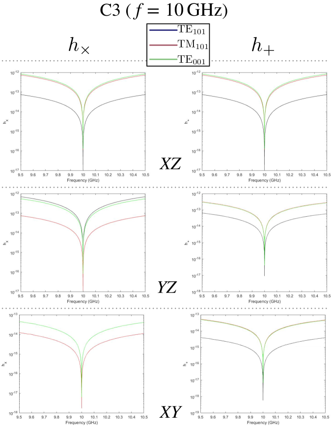
In this section we compute the sensitivities assuming that the GW impinges with the angle which generates the maximum coupling between the GW and the cavity mode, as reported in table 3. In order to perform realistic numerical calculations we use the data from different magnet facilities for each cavity which have been described in table 4. Therefore, we will assume that the cavity C1 might be introduced in a magnet test-bed similar to KLOE (KLASH) [52] [54], where the external magnetostatic field is T and the system temperature is K. The detection bandwidth used in the simulations is kHz conforming the cavity loaded quality factor , MHz being the resonance frequency. We have used in the simulations a detection time ms, and a signal-to-noise ratio for all the cavities. This short detection time is key to access some of the signals that may be present in the studied frequency band [25]. An important remark is that in some previous studies (as in [25]) a longer integration of s time has been considered. To compare our results with those of these studies, recall that the constrain in the maximum allowed GW amplitud grows as with . The sensitivity for the cavity C1 has been plotted in figure 7 using (4.7), observing that the minimum detected amplitude is around . We have also computed the sensitivity curves of the cavities C2 and C3 in figure 8 and figure 9, respectively. The magnet chosen for these two cavities is the Oxford-Leiden one from CAPP (see table 3 for details) [53]. For these cases the minimum detected amplitude is for C2, and for C3. It is evident that these values are far from those expected from different models of GWs in this band [23, 19]. Still, it is important to consider that those are first steps in this emerging field, where neither the cavity design nor the readout system are optimized. We will come back to possible improvements in section 5. It is also very relevant that our results are on the bulk part of other methods suggested to detect similar GWs at these high frequencies [19, 23].
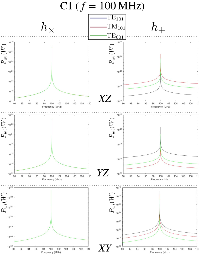
Figure 10 depicts the detected GWs power as a function of frequency in the three coaxial probes of the cavity C1 for the same optimal sensitivities in figure 7. It is worth noting that, in the case of cross polarization, the detected power level is around W, which is consistent with the expected level of power estimated in dark matter axion studies [45]. However, for the analyzed scenarios, the plus polarization exhibits greater observed power levels, with values around W. This means that we are mainly sensitive to one polarization, at least with the proposed cubic cavity and incoming directions described in this work. In the future, we will study how this statement is modified in generic directions for the incoming GW.
It is important to emphasize at this point that in the frequency response computations we have not used the classical Lorentzian approach for describing the frequency resonant curves; on the contrary, the BI-RME 3D theory provides the wide-band exact solution of the cavity electrical response.
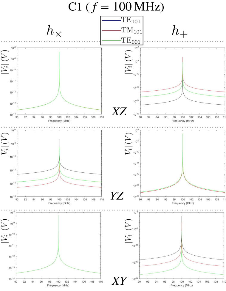
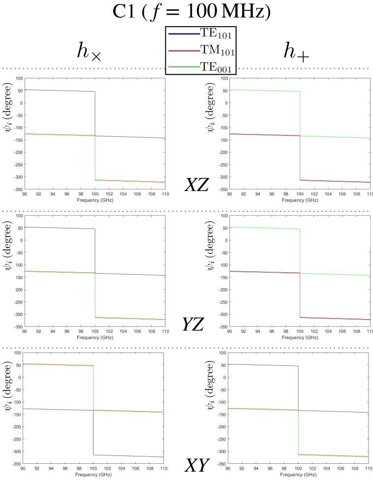
As indicated in section 3, the BI-RME 3D method is capable of computing the complex values of voltages in the cavity ports for the ranges of frequencies under study. Figures 11 and 12 show, respectively, the magnitude and phase for detected voltages, , as a function of frequency in the three coaxial probes of the cavity C1 around its resonant frequency ( MHz). As expected from figure 10, voltages detected from plus polarization are higher than those ones produced by cross polarization. In fact, plus polarization voltages show maximum values around V while cross polarization ones are around V. Moreover, all of the degenerate modes and GW polarizations exhibit very similar behavior for voltage phase values, with a phase shift at the resonant frequency. For the purpose of concision, the phase differences between port signals are not displayed in this paper; however, they reveal very similar behaviours in both polarizations, not showing phase shifts at the resonant frequency. Additionally, it should be noted that the detected phase values vary with GW polarization and incident planes, suggesting that GW polarizations and incident angles may be detected with this type of cavities.
5 Conclusions and future research lines
The BIRME 3D method has been adapted in this work to analyze the detection of GWs by means of microwave resonant cavities. Whilst the classical analysis of these cavities with numerical methods (finite elements or finite differences) provide scattering parameters or eigenvalues / eigenvectors that only allow to obtain the resonance characteristics (resonant frequency, loaded and unloaded quality factor, and the form factor), this new formulation is able to introduce the source, that is, the GW induced current , and to obtain the magnitude and phase of the signal produced by the GWs at the output ports of the cavity. On one hand, this allows one to precisely obtain the detected power or voltage responses over a wide frequency range, obviating the need for Cauchy-Lorentz approximations. On the other hand, this analysis method enables, for the first time, the acquisition of the phases of the signals in the output ports, which may be a crucial consideration when attempting to develop GW microwave-cavity detectors that operate with interferometric methods among various cavities. If one considers shortly lived GWs, the detection time in the receiver cannot be increased too much, and interferometry may be a powerful technique for getting better sensitivities.
This formulation has been applied to a cubic cavity with three perpendicular ports which allow for the simultaneous detection of the three degenerate modes , and . It has been shown that, in some cases, the combination of two modes increases the range of incident angles that can be explored while maintaining high coupling levels. This range is complete for the plane case. For and planes, possible solutions for avoiding blind angles are introducing a second cavity (rotated with regards to the first one) or performing a rotation of the cavity inside the magnet. Both actions lead to a rotation of the external magnetic field inside the cavity. Notice also that the natural rotation of the Earth would improve this situation for signals persisting for hours.
It has been confirmed that the coupling of the GW with the cavity modes is much more complex than the axion one. In the latter, there exist a clear dominant mode with optimal form factor, but for GWs any mode, regardless of its polarization, can get an adequate coupling, depending on the incident angle and on the frequency. This motivates the determination of how the the detection can be improved by combining the extracted signals from different modes. In an alternative operation mode, by detuning degenerate modes and probing other higher order modes, a set of frequencies (one per mode) can be explored in parallel. Another key difference that we have not remarked until now is that the tuning of the signal to a resonant mode of the cavity may happen naturally for GWs, without the need for a scanning strategy. This is because when black hole binaries emit GWs in this range, their orbital motion typically evolves fast enough to explore the frequencies of interest in their emitted signal in a relatively short time. In this sense, by focusing on integration times of ms, one expects the narrow resonances shown in figures 7-9 to be excited during the merger event. In the future we plan to study the effect of considering the frequency spectrum of a GW using the formulation developed in this work.
Although this work has been done on a relatively basic rectangular-section microwave cavity, it can be readily expanded to other cavities with superior performance characteristics, such as cylindrical, spherical, or other mixed geometries like rectangular cavities with bended edges, reducing losses at the edges and so improving the quality factor. Moreover, although the simulations show detected voltage and power levels still far from expected signals, the presented setup is a first step for GW detection for a wide range of incident angles. Further improvements can be put in place to work towards a more relevant sensitivity. First, the cavity performance indicator, [25], can be improved following the main lines currently in development by the axion detection community. For instance, a better quality factor can be achieved by using magnetic-resilient superconductor materials [55, 56] or dielectric materials [57], maintaining the three degenerate modes. Another critical aspect for the cavity design in future works will be the introduction of a tuning system that affects in the same way the three degenerate modes. Remarkably, this tuning system may also be used to control the splitting of these modes, which may serve as a way to detect GWs of much lower frequencies, following the ideas333These ideas are based on cavities loaded with a mode, that is transformed into another one by the arrival of GWs. We leave the precise study of these set-ups for future works. in [58, 22]. Furthermore, it would be very relevant to reduce the noise in the haloscope system by means of photon detection devices, as qubits, already proposed for dark photon detection [59], although magnetic resilience is still not developed.
Acknowledgments
We thank to Camilo García-Cely for helpful comments and discussions as well as for his support in the calculation of the effective induced currents. We are also grateful to Valerie Domcke, Claudio Gatti and Nick Rodd for comments on a previous draft.
This work was performed within the RADES group; we thank our colleagues for their support.
It has been funded by MCIN/AEI/10.13039/501100011033/ and by “ERDF A way of making Europe”, under grants PID2019-108122GB-C33, PID2022-137268NB-C53, PID2022-137268NA-C55, and PID2020-115845GB-I00. Generalitat Valenciana has also funded this work under the project ASFAE/2022/013. This article is based upon work from COST Action COSMIC WISPers CA21106, supported by COST (European Cooperation in Science and Technology). IFAE is partially funded by the CERCA program of the Generalitat de Catalunya. Diego Blas acknowledges the support from the Departament de Recerca i Universitats de la Generalitat de Catalunya al Grup de Recerca i Universitats from Generalitat de Catalunya to the Grup de Recerca 00649 (Codi: 2021 SGR 00649).
References
- [1] LIGO Scientific, Virgo collaboration, Observation of Gravitational Waves from a Binary Black Hole Merger, Phys. Rev. Lett. 116 (2016) 061102 [1602.03837].
- [2] M. Maggiore, Gravitational Waves. Vol. 1: Theory and Experiments, Oxford Master Series in Physics, Oxford University Press (2007).
- [3] J. Antoniadis et al., The second data release from the European Pulsar Timing Array III. Search for gravitational wave signals, 2306.16214.
- [4] D.J. Reardon et al., Search for an Isotropic Gravitational-wave Background with the Parkes Pulsar Timing Array, Astrophys. J. Lett. 951 (2023) L6 [2306.16215].
- [5] NANOGrav collaboration, The NANOGrav 15 yr Data Set: Evidence for a Gravitational-wave Background, Astrophys. J. Lett. 951 (2023) L8 [2306.16213].
- [6] H. Xu et al., Searching for the Nano-Hertz Stochastic Gravitational Wave Background with the Chinese Pulsar Timing Array Data Release I, Res. Astron. Astrophys. 23 (2023) 075024 [2306.16216].
- [7] T. Namikawa, S. Saga, D. Yamauchi and A. Taruya, CMB Constraints on the Stochastic Gravitational-Wave Background at Mpc scales, Phys. Rev. D 100 (2019) 021303 [1904.02115].
- [8] LISA collaboration, Laser Interferometer Space Antenna, 1702.00786.
- [9] S. Hild et al., Sensitivity Studies for Third-Generation Gravitational Wave Observatories, Class. Quant. Grav. 28 (2011) 094013 [1012.0908].
- [10] M. Punturo et al., The Einstein Telescope: A third-generation gravitational wave observatory, Class. Quant. Grav. 27 (2010) 194002.
- [11] LIGO Scientific collaboration, Exploring the Sensitivity of Next Generation Gravitational Wave Detectors, Class. Quant. Grav. 34 (2017) 044001 [1607.08697].
- [12] L. Badurina et al., AION: An Atom Interferometer Observatory and Network, JCAP 05 (2020) 011 [1911.11755].
- [13] MAGIS-100 collaboration, Matter-wave Atomic Gradiometer Interferometric Sensor (MAGIS-100), Quantum Sci. Technol. 6 (2021) 044003 [2104.02835].
- [14] AEDGE collaboration, AEDGE: Atomic Experiment for Dark Matter and Gravity Exploration in Space, EPJ Quant. Technol. 7 (2020) 6 [1908.00802].
- [15] K. Yagi and N. Seto, Detector configuration of DECIGO/BBO and identification of cosmological neutron-star binaries, Phys. Rev. D 83 (2011) 044011 [1101.3940].
- [16] A. Sesana et al., Unveiling the gravitational universe at -Hz frequencies, Exper. Astron. 51 (2021) 1333 [1908.11391].
- [17] D. Blas and A.C. Jenkins, Bridging the Hz Gap in the Gravitational-Wave Landscape with Binary Resonances, Phys. Rev. Lett. 128 (2022) 101103 [2107.04601].
- [18] M.A. Fedderke, P.W. Graham and S. Rajendran, Asteroids for Hz gravitational-wave detection, Phys. Rev. D 105 (2022) 103018 [2112.11431].
- [19] N. Aggarwal et al., Challenges and opportunities of gravitational-wave searches at MHz to GHz frequencies, Living Rev. Rel. 24 (2021) 4 [2011.12414].
- [20] M. Gertsenshtein, Wave resonance of light and gravitional waves, Sov Phys JETP 14 (1962) 84.
- [21] M.E. Gertsenshtein and V.I. Pustovŏit, On the detection of low frequency gravitational waves, J. Exptl. Theoret. Phys. 43 (1962) .
- [22] A. Berlin, D. Blas, R. Tito D’Agnolo, S.A.R. Ellis, R. Harnik, Y. Kahn et al., Electromagnetic cavities as mechanical bars for gravitational waves, Phys. Rev. D 108 (2023) 084058 [2303.01518].
- [23] V. Domcke, Electromagnetic high-frequency gravitational wave detection, in 57th Rencontres de Moriond on Electroweak Interactions and Unified Theories, 6, 2023 [2306.04496].
- [24] N. Herman, A. Füzfa, L. Lehoucq and S. Clesse, Detecting planetary-mass primordial black holes with resonant electromagnetic gravitational-wave detectors, Phys. Rev. D 104 (2021) 023524 [2012.12189].
- [25] A. Berlin, D. Blas, R. Tito D’Agnolo, S.A.R. Ellis, R. Harnik, Y. Kahn et al., Detecting high-frequency gravitational waves with microwave cavities, Phys. Rev. D 105 (2022) 116011 [2112.11465].
- [26] V. Domcke, C. Garcia-Cely, S.M. Lee and N.L. Rodd, Symmetries and Selection Rules: Optimising Axion Haloscopes for Gravitational Wave Searches, 2306.03125.
- [27] G. Conciauro, M. Guglielimi and R. Sorrentino, Advanced Modal Analysis. CAD Techniques for Waveguide Components and Filters, John Wiley and Sons, Ltd, first ed. (2000).
- [28] V. Domcke, C. Garcia-Cely and N.L. Rodd, Novel Search for High-Frequency Gravitational Waves with Low-Mass Axion Haloscopes, Phys. Rev. Lett. 129 (2022) 041101 [2202.00695].
- [29] J. Jin, The Finite Element Method in Electromagnetics, John Wiley & Sons, Inc., second ed. (2002).
- [30] M. Salazar-Palma, T.K. Sarkar, L.-E. García-Castillo and A. Djordjević, Iterative and Self-Adaptative Finite-Elements in Electromagnetic Modeling, Artech House, Inc., first ed. (1998).
- [31] S.C.H. Allen Taflove, Computational Electrodynamics. The Finite-Difference Time-Domain Method, Artech House, Inc., second ed. (2000).
- [32] T. Itoh, Numerical techniques for microwave and millimeter-wave passive structures, John Wiley and Sons, Inc., first ed. (1989).
- [33] “CST STUDIO SUITE, https://www.3ds.com/products-services/simulia/products/cst-studio-suite/.”
- [34] “ANSYS HFSS, https://www.ansys.com/products/electronics/ansys-hfss.”
- [35] “COMSOL MULTIPHYSICS, https://www.comsol.com/.”
- [36] R.F. Harrington, Field Computation by Moment Methods, IEEE Press, first ed. (1993).
- [37] G.W. Hanson and A.B. Yakovlev, Operator Theory for Electromagnetics. An introduction, Springer-Verlag, first ed. (2002).
- [38] C.-T. Tai, Dyadic Green Functions in Electromagnetic Theory, IEEE Press, second ed. (1994).
- [39] P. Arcioni, M. Bressan and L. Perregrini, A new boundary integral approach to the determination of resonant modes of arbitrarily shaped cavities, IEEE Transactions on Microwave Theory and Techniques MTT-43 (1995) 1848 .
- [40] P. Arcioni, M. Bozzi, M. Bressan, G. Conciauro and L. Perregrini, Frequency/time-domain modelling of 3d waveguide structures by a bi-rme approach, International Journal of Numerical Modeling 15 (2002) 3 .
- [41] F. Mira, M. Bressan, G. Conciauro, B. Gimeno and V. Boria, Fast s-domain modeling of rectangular waveguides with radially symmetric metal insets, IEEE Transactions on Microwave Theory and Techniques 53 (2005) 1294 .
- [42] Ángel A. San Blas, F. Mira, V.E. Boria, B. Gimeno, M. Bressan and P. Arcioni, On the fast and rigorous analysis of compensated waveguide junctions using off-centered partial-height metallic posts, IEEE Transactions on Microwave Theory and Techniques 55 (2007) 168 .
- [43] P. Arcioni, M. Bozzi, M. Bressan, G. Conciauro and L. Perregrini, The bi-rme method: an historical overview, 2014 International Conference on Numerical Electromagnetic Modeling and Optimization for RF, Microwave, and Terahertz Applications (NEMO) (2014) .
- [44] C.-T. Tai, Generalized Vector and Dyadic Analysis. Applied Mathematics in Field Theory, IEEE Press, first ed. (1991).
- [45] P. Navarro, B. Gimeno, A. Álvarez Melcón, S.A. Cuendis, C. Cogollos, A. Díaz-Morcillo et al., Wide-band full-wave electromagnetic modal analysis of the coupling between dark-matter axions and photons in microwave resonators, Physics of the Dark Universe 36, 101001 (2022) .
- [46] R.E. Collin, Foundations for Microwave Engineering, McGraw-Hill, Inc., second ed. (1992).
- [47] D.M. Pozar, Microwave Engineering, John Wiley and Sons, Ltd, fourth ed. (2012).
- [48] J.V. Bladel, Electromagnetic Fields, IEEE Press, second ed. (2007).
- [49] R.E. Collin, Field Theory of Guided Waves, IEEE Press, second ed. (1991).
- [50] S. Cogollos, V. Boria, P. Soto, B. Gimeno and M. Guglielmi, Efficient cad tool for inductively coupled rectangular waveguide filters with rounded corners, 2001 31st European Microwave Conference (2001) .
- [51] “MATLAB, https://mathworks.com/products/matlab.html.”
- [52] D. Alesini, D. Babusci, P. Beltrame S. J., F. Björkeroth, F. Bossi, P. Ciambrone et al., KLASH Conceptual Design Report, 1911.02427.
- [53] A.K. Yi, S. Ahn, Çağlar Kutlu, J. Kim, B.R. Ko, B.I. Ivanov et al., Axion dark matter search around 4.55 microev with dine-fischler-srednicki-zhitnitskii sensitivity, Phys. Rev. Lett. 130, 071002 (2023) .
- [54] D. Alesini, D. Babusci, P. Beltrame, F. Bossi, P. Ciambrone, A. D’Elia et al., The future search for low-frequency axions and new physics with the FLASH resonant cavity experiment at Frascati National Laboratories, Physics of the Dark Universe 42, 101370 (2023) .
- [55] S. Posen, M. Checchin, O.S. Melnychuk, T. Ring, I. Gonin and T. Khabiboulline, High-Quality-Factor Superconducting Cavities in Tesla-Scale Magnetic Fields for Dark-Matter Searches, Phys. Rev. Applied 20 (2023) 034004 [2201.10733].
- [56] D. Ahn, O. Kwon, W. Chung, W. Jang, D. Lee, J. Lee et al., Superconducting cavity in a high magnetic field, 2002.08769.
- [57] R. Di Vora et al., High-Q Microwave Dielectric Resonator for Axion Dark-Matter Haloscopes, Phys. Rev. Applied 17 (2022) 054013 [2201.04223].
- [58] R. Ballantini et al., Microwave apparatus for gravitational waves observation, gr-qc/0502054.
- [59] A.V. Dixit, S. Chakram, K. He, A. Agrawal, R.K. Naik, D.I. Schuster et al., Searching for Dark Matter with a Superconducting Qubit, Phys. Rev. Lett. 126 (2021) 141302 [2008.12231].