A Simple and Scalable Representation
for Graph Generation

Abstract

Recently, there has been a surge of interest in employing neural networks for graph generation, a fundamental statistical learning problem with critical applications like molecule design and community analysis. However, most approaches encounter significant limitations when generating large-scale graphs. This is due to their requirement to output the full adjacency matrices whose size grows quadratically with the number of nodes. In response to this challenge, we introduce a new, simple, and scalable graph representation named gap encoded edge list (GEEL) that has a small representation size that aligns with the number of edges. In addition, GEEL significantly reduces the vocabulary size by incorporating the gap encoding and bandwidth restriction schemes. GEEL can be autoregressively generated with the incorporation of node positional encoding, and we further extend GEEL to deal with attributed graphs by designing a new grammar. Our findings reveal that the adoption of this compact representation not only enhances scalability but also bolsters performance by simplifying the graph generation process. We conduct a comprehensive evaluation across ten non-attributed and two molecular graph generation tasks, demonstrating the effectiveness of GEEL.

1 Introduction

Learning the distribution over graphs is a challenging problem across various domains, including social network analysis (Grover et al., 2019) and molecular design (Li et al., 2018; Maziarka et al., 2020). Recently, neural networks gained much attention in addressing this challenge by leveraging the advancements in deep generative models, e.g., diffusion models (Ho et al., 2020), to show promising results. These works are further categorized based on the graph representations they employ.

However, the majority of the graph generative models do not scale to large graphs, since they generate the adjacency matrix-based graph representations (Simonovsky & Komodakis, 2018; Madhawa et al., 2019; Liu et al., 2021; Maziarka et al., 2020). In particular, for large graphs with $N$ nodes, the adjacency matrix is hard to handle since they consist of $N^{2}$ binary elements. For example, employing a Transformer-based autoregressive model for all the binary elements requires $O(N^{4})$ computational complexity. Researchers have considered tree-based (Segler et al., 2018) or motif-based representations (Jin et al., 2018; 2020) to mitigate this issue, but these representations constrain the graphs being generated, e.g., molecules or graphs with motifs extracted from training data.

Intriguingly, a few works (Goyal et al., 2020; Bacciu & Podda, 2021) have considered generating the edge list representations as a potential solution for large-scale graph generation. In particular, the list contains $M$ edges that are fewer than $N^{2}$ elements in the adjacency matrix, a distinctive difference especially for sparse graphs. However, such edge list-based graph generative models instead suffer from the vast vocabulary size $N^{2}$ for the possible edges. Consequently, they face the challenge of learning dependencies over a larger output space and may overfit to a specific edge or an edge combination appearing only in a few samples. Indeed, the edge list-based representations empirically perform even worse than simple adjacency matrix-based models (You et al., 2018), e.g., see Table 1.

In this paper, we propose a simple, scalable, yet effective graph representation for graph generation, coined Gap Encoded Edge List (GEEL). On one hand, grounded in edge lists, GEEL enjoys a compact representation size that aligns with the number of edges. On the other hand, GEEL improves the edge list representations by significantly reducing the vocabulary size with gap encodings that replace the node indices with the difference between nodes, i.e., gap, as described in Figure 1(a). We also promote bandwidth restriction (Diamant et al., 2023) which further reduces the vocabulary size. Next, we augment the GEEL generation with node positional encoding. Finally, we introduce a new grammar for the extension of GEEL to attributed graphs.

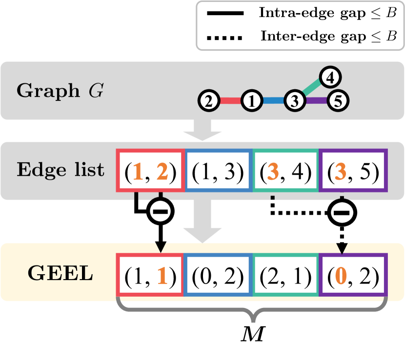
(a) Overview.

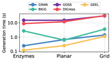
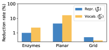
(b) Short inference time.

(c) Rep. and vocab. size reduction.

Figure 1: Overview and advantages of gap encoded edge list (GEEL).

The advantages of our GEEL are primarily twofold: scalability and efficacy. First, regarding scalability, the reduced representation and the vocabulary sizes mitigate the computational and memory complexity, especially for sparse graphs, as described in Figure 1(c). Second, concerning the efficacy, GEEL narrows down the search space to $B^{2}$ via intra- and inter-edge gap encodings, where the size of each gap is bounded by graph bandwidth $B$ (Chinn et al., 1982). We reduce this parameter via the bandwidth restriction scheme (Diamant et al., 2023). This prevents the model from learning dependencies among a vast vocabulary of size $N^{2}$. This improvement is more pronounced when compared with the existing edge list representations, as described in Figure 1(c).

We present an autoregressive graph generative model to generate the proposed GEEL with node positional encoding. In detail, we observe that a simple LSTM (Hochreiter & Schmidhuber, 1997) combined with the proposed GEEL exhibits $O(M)$ complexity. Furthermore, combined with the node positional encoding that indicates the current node index, our GEEL achieved superior performance across ten general graph benchmarks while maintaining simplicity and scalability.

We further extend GEEL to attributed graphs by designing a new grammar and enforcing it to filter out invalid choices during generation. Specifically, our grammar specifies the position of node- and edge-types to be augmented in the GEEL representation. This approach led to competitive performance for two molecule generation benchmarks.

In summary, our key contributions are as follows:

• We newly introduce GEEL, a simple and scalable graph representation that has a compact representation size of $M$ based on edge lists while reducing the large vocabulary size $N^{2}$ of the edge lists to $B^{2}$ by applying gap encodings. We additionally reduce the graph bandwidth $B$ by the C-M ordering following Diamant et al. (2023).

• We propose to autoregressively generate GEEL by incorporating node positional encoding and combining it with an LSTM of $O(M)$ complexity.

• We extend GEEL to deal with attributed graphs by designing a new grammar that takes the node- and edge-types into account.

• We validate the efficacy and scalability of the proposed GEEL and the resulting generative framework by showing the state-of-the-art performance on twelve graph benchmarks.

2 Related work

Adjacency matrix-based graph representation. The adjacency matrix is the most prevalent graph representation, capturing straightforward pairwise relationships between nodes (Simonovsky & Komodakis, 2018; Jo et al., 2022; Vignac et al., 2022; You et al., 2018; Niu et al., 2020; Shi et al., 2020; Luo et al., 2021). For instance, You et al. (2018) proposed autoregressive generative models, Luo et al. (2021); Shi et al. (2020) presented normalizing flow models, and Jo et al. (2022) applied score-based models for graph generation. However, these methods suffer from the large representation size associated with generating the full adjacency matrix, which is impractical for large-scale graphs.

To solve this problem, several works have introduced scalable graph generative models (Liao et al., 2019; Dai et al., 2020; Diamant et al., 2023). Specifically, Liao et al. (2019) proposed a block-wise generation which enabled efficiency-quality trade-off. Dai et al. (2020) proposed to avoid consideration of every entry in the adjacency matrix, leveraging on the sparsity of graphs. Finally, Diamant et al. (2023) proposed to constrain the bandwidth via C-M ordering for any graph generative models, bypassing the generation of out-of-bandwidth elements, which reduces the representation complexity to $NB$.

Tree-based graph representation. Researchers have developed tree-based representations by employing tree search algorithms (Segler et al., 2018; Ahn et al., 2022). Specifically, Segler et al. (2018) employed SMILES, a sequential representation for molecules, constructed from the DFS traversal of molecular graphs with omitted cycles. Complementing this, Ahn et al. (2022) designed a new representation that exploits the inherent tree-like structure of molecules.

Motif-based graph representation. Researchers have investigated motif-based representations (Jin et al., 2018; 2020; Guo et al., 2022), aiming to capture meaningful subgraphs with lower computational costs. In detail, Jin et al. (2018; 2020) focused on extracting common fragments from datasets. Since these techniques rely on domain-specific knowledge, Guo et al. (2022) introduced a domain-agnostic methodology to learn motif-based vocabulary by running reinforcement learning. However, it is still restricted to generating graphs with seen motifs that are included in the training set.

Edge list-based graph representation. A few works have presented edge list-based representations (Goyal et al., 2020; Bacciu & Podda, 2021). Employing an edge list as a graph representation reduces the representation size to $M$, which is smaller than that of the adjacency matrix, $N^{2}$. However, these methods suffer from the large vocabulary size $N^{2}$, resulting in a large search space and subsequently degrading the generation quality. They also face difficulties in capturing long-term dependencies due to their reliance on depth-first search (DFS) traversal for edge construction. Specifically, DFS traversal fails to closely place edges connected to the same node, so the model must span a broader range of steps to account for edges connected to the same node.

3 Method

In this section, we introduce our new graph representation, termed gap encoded edge list (GEEL), and the autoregressive generation process using GEEL. GEEL has a small representation size $M$ by employing edge lists. In addition, GEEL enjoys a reduced vocabulary size with gap encodings and bandwidth restriction, narrowing down the search space and resulting in the generation of high-quality graphs.

3.1 Gap encoded edge list representation (GEEL)

First, we present our GEEL representation, which leverages the small representation size of edge lists and the reduced vocabulary size with gap encoding and bandwidth restriction. Consider a graph with $N$ nodes, $M$ edges, and graph bandwidth $B$ (Chinn et al., 1982). The associated edge list has a representation size of $M$ which is smaller compared to the size of the adjacency matrix $N^{2}$. However, it has a large vocabulary size of $N^{2}$, consisting of tuples of node indices. To address this, we reduce the vocabulary size into $B^{2}$ by replacing the node indices in the original edge list with gap encodings as illustrated in Figure 1(a). We encode two types of gaps: (1) the intra-edge gap between the source and the target nodes and (2) the inter-edge gap between source nodes in a pair of consecutive edges.

To this end, consider a connected undirected graph $G=(\mathcal{V},\mathcal{E})$ with $N$ nodes and $M$ edges. We define the ordering as an invertible mapping $\pi:\mathcal{V}\rightarrow\{1,\ldots,N\}$ from a vertex into its rank for a particular order of nodes. Then we define the edge list $\tau_{\text{EL}}$ as a sequence of pairs of integers:

$$\tau_{\text{EL}}=(s_{1},t_{1}),(s_{2},t_{2}),\ldots,(s_{M},t_{M}),$$

where $s_{m},t_{m}\in\{1,\ldots,N\}$ are the $m$-th source and target node indices that satisfy $(\pi^{-1}(s_{m}),\pi^{-1}(t_{m}))\in\mathcal{E}$, respectively. Without loss of generality, we assume that $s_{m}<t_{m}$ and the edge list is sorted with respect to the ordering, i.e., if $m<\ell$, then $s_{m}<s_{\ell}$ or $s_{m}=s_{\ell},t_{m}<t_{\ell}$. For example, $(1,2),(1,3),(2,3),(3,5)$ is a sorted edge list while $(1,2),(2,3),(3,5),(1,3)$ is not.

Consequently, we define our GEEL $\tau_{\text{GEEL}}$ as a sequence of gap encoding pairs as follows:

$$\tau_{\text{GEEL}}=(a_{1},b_{1}),(a_{2},b_{2}),\ldots,(a_{M},b_{M}),$$

where $a_{m}$ and $b_{m}$ are the inter- and intra-edge gap encodings, respectively. To be specific, the inter-edge gap encoding indicates the difference between consecutive source indices as follows:

$$a_{m}=s_{m}-s_{m-1},\qquad m=1,\ldots,M,\qquad s_{0}=0.$$

Furthermore, the intra-edge gap encoding $b_{m}$ indicates the difference between the associated source and target node indices as follows:

$$b_{m}=t_{m}-s_{m},\qquad m=1,\ldots,M.$$

Then one can recover the original edge list $\tau_{\text{EL}}$ from GEEL $\tau_{\text{GEEL}}$ as follows:

$$s_{m}=\sum_{\ell=1}^{m}a_{\ell},\qquad t_{m}=b_{m}+\sum_{\ell=1}^{m}a_{\ell}.$$

Note that the gap encodings are always positive and GEEL can be generalized to directed graphs by allowing negative intra-edge gap encodings.

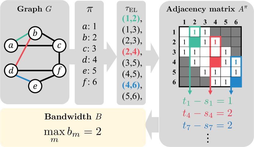
Figure 2: Bandwidth of an adjacency matrix.

Reduction of the vocabulary size. In training a generative model for edge lists and GEEL, the vocabulary size of $(s_{m},t_{m})$ and $(a_{m},b_{m})$ determines the complexity of the model. Here, we show that the vocabulary size of our GEEL is $B^{2}$ for the graph bandwidth $B$, which is smaller than the vocabulary size $N^{2}$ of the original edge list representation. Many real-world graphs, such as molecules and community graphs, exhibit low bandwidths as shown in Appendix C and by Diamant et al. (2023).

The vocabulary size of our GEEL representation is bounded by $\max_{m}a_{m}\cdot\max_{m}b_{m}$. On one hand, the maximum intra-edge gap encoding coincides with the definition of the graph bandwidth, i.e., the maximum difference between a pair of adjacent nodes, denoted as $\max_{m}b_{m}=B$ (Figure 2 illustrates the definition). On the other hand, we can obtain the following upper bound for the inter-edge encoding:

$$\max_{m}a_{m}=\max_{m}(s_{m}-s_{m-1})\leq\max_{m}\left(\max_{\ell<m}t_{\ell}-s_{m-1}\right)\leq\max_{m}\max_{\ell<m}\left(t_{\ell}-s_{\ell}\right)\leq B,$$

where the first inequality is based on deriving $s_{m}\leq\max_{\ell<m}t_{\ell}$ from the graph connectivity constraint: each source node index $s_{m}$ must appear as a target node index in prior for the graph to be connected, i.e., $s_{m}=t_{\ell}$ for some $\ell<m$. Consequently, the vocabulary size of our GEEL representation is upper-bounded by $\max_{m}a_{m}\cdot\max_{m}b_{m}\leq B^{2}$.

Given that the vocabulary size of GEEL is bounded by $B^{2}$, small bandwidth benefits graph generation by reducing the computational cost and the search space. We follow Diamant et al. (2023) to restrict the bandwidth via the Cuthill-McKee (C-M) node ordering (Cuthill & McKee, 1969). We also provide an ablation study with various node orderings in Section 4.3.

3.2 Autoregressive generation of GEEL and node positional encoding

Autoregressive generation. We first describe our method for the autoregressive generation of GEEL. To this end, we propose to maximize the evidence lower bound of the log-likelihood with respect to the latent ordering. To be specific, following prior works on autoregressive graph generative models (You et al., 2018; Liao et al., 2019; Dai et al., 2020), we maximize the following lower bound:

$$\log p(G)\geq\mathbb{E}_{q(\pi|G)}[\log p(G,\pi)]+C,$$

where $C$ is a constant and $q(\pi|G)$ is a variational posterior of the ordering given the graph $G$. Under this framework, our choice of choosing the C-M ordering for each graph corresponds to a choice of the variational distribution $q(\pi|G)$. Fixing a particular ordering for each graph yields the maximum log-likelihood objective for $\log p(G,\pi)=\log p(\tau_{\text{GEEL}})$.

We generate GEEL using an autoregressive model formulated as follows:

$$p(\tau_{\text{GEEL}})=p(a_{1},b_{1})\prod_{m=2}^{M}p(a_{m},b_{m}|\{a_{\ell}\}_{\ell=1}^{m-1},\{b_{\ell}\}_{\ell=1}^{m-1}).$$

Notably, we treat each tuple $(a_{m},b_{m})$ as one token and generate a token at each step. Similar to text generative models, we also introduce the begin-of-sequence (BOS) and the end-of-sequence (EOS) tokens to indicate the start and end of the sequence generation process, respectively (Collins, 2003).

Finally, it is noteworthy that we train a long short-term memory (LSTM) model (Hochreiter & Schmidhuber, 1997) to minimize the proposed objective. Adopting LSTM as our backbone ensures an $O(M)$ complexity for our generative model, due to the linear complexity of the LSTM. The model architecture can be freely changed to other architectures such as Transformers (Vaswani et al., 2017), as demonstrated in Section 4.3.

Source node positional encoding. While the gap encoding allows a significant reduction in vocabulary size, it also complicates the inherent semantics since each source node index is represented by the cumulative summation over the intra-edge gap encodings. Instead of burdening the generative model to learn the cumulative summation, we directly supplement the token embeddings with the node positional encoding of the source node index, i.e., $\sum_{\ell=1}^{m}a_{\ell}$ at the $(m+1)$-th step as:

$$\phi\big{(}(a_{m},b_{m})\big{)}=\phi_{\operatorname{tuple}}\big{(}(a_{m},b_{m})\big{)}+\phi_{\operatorname{PE}}\Big{(}\sum_{\ell=1}^{m}a_{\ell}\Big{)},$$

where $\phi$ is the final embedding, $\phi_{\operatorname{tuple}}$ is the token embedding, and $\phi_{\operatorname{PE}}$ is the positional encoding.

3.3 GEEL for attributed graphs

In this section, we elaborate on the extension of GEEL to attributed graphs. To this end, we augment the GEEL representation with node- and edge-types. Our attributed GEEL follows a specific grammar that filters out invalid choices of tokens.

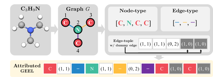
Figure 3: An example of attributed GEEL. The colored parts of the attributed GEEL denote the node features (i.e., C and N) and edge features (i.e., single bond -). The shaded parts denote the self-loops added to the original GEEL, where self-loops are added to the nodes that are not connected to the nodes with larger node indices (i.e., nodes with indices 3 and 4).

Grammar of attributed GEEL. For the generation of attributed graphs with node- and edge-types, we not only generate the edge-tuples $(a_{k},b_{k})$ as in Section 3.1 but also generate node- and edge-types according to the following rules. We provide an illustrative example of attribute GEEL in Figure 3.

• Before describing edge-tuples starting with a new source node, add the paired node-type.

• After adding an edge-tuple, add the paired edge-type.

One can observe that our rules are intuitive: for each source node, we first describe the node-type and then generate the associated edge-tuple and types. For nodes that are not associated with any edge-tuple as a source node, we add a “dummy” edge-tuple with the node as its source. As a result, our representation size for attributed graphs is at most $2M+N$ and the vocabulary size is $2B+|X|+|E|$ where $|X|$ denotes the number of node features and $|E|$ denotes the number of edge features.

Autoregressive generation with grammar constraints. To enforce the attribute grammar, we introduce an algorithm to filter out invalid choices of tokens.

• The first token is always the node-type token.

• The node-type tokens are always followed by edge-tuple tokens.

• The edge-tuple tokens are always followed by edge-type tokens.

• The edge-type tokens are always followed by node-type tokens or edge-tuple tokens.

Table 1: General graph generation performance. The baseline results are from prior works (Jo et al., 2022; Kong et al., 2023; Martinkus et al., 2022; Dai et al., 2020; Diamant et al., 2023) or obtained by running the open-source codes. Note that OOM indicates Out-Of-Memory and N.A. for BwR indicates that the generated samples are all invalid. For each metric, the numbers that are superior or comparable to the MMD of the training graphs are highlighted in bold. The comparability is determined by whether the MMD falls within one standard deviation.

	Planar			Lobster			Enzymes			SBM
	$|V|=64$			$10\leq|V|\leq 100$			$10\leq|V|\leq 125$			$31\leq|V|\leq 187$
Method	Deg.	Clus.	Orb.	Deg.	Clus.	Orb.	Deg.	Clus.	Orb.	Deg.	Clus.	Orb.
Training	0.001	0.002	0.000	0.005	0.000	0.007	0.006	0.018	0.007	0.016	0.002	0.047
GraphVAE	-	-	-	-	-	-	1.369	0.629	0.191	-	-	-
GraphRNN	0.005	0.278	1.254	0.000	0.000	0.000	0.017	0.062	0.046	0.006	0.058	0.079
GRAN	0.001	0.043	0.001	0.038	0.000	0.001	0.023	0.031	0.169	0.011	0.055	0.054
EDP-GNN	-	-	-	-	-	-	0.023	0.268	0.082	-	-	-
GraphGen	1.762	1.423	1.640	0.548	0.040	0.247	0.146	0.079	0.054	1.230	1.752	0.597
GraphGen-Redux	1.105	1.809	0.517	1.189	1.859	0.885	0.456	0.035	0.251	-	-	-
GraphAF	-	-	-	-	-	-	1.669	1.283	0.266	-	-	-
GraphDF	-	-	-	-	-	-	1.503	1.283	0.266	-	-	-
BiGG	0.002	0.004	0.000	0.000	0.000	0.000	0.010	0.018	0.011	0.029	0.003	0.036
GDSS	0.250	0.393	0.587	0.117	0.002	0.149	0.026	0.061	0.009	0.496	0.456	0.717
DiGress	0.000	0.002	0.008	0.021	0.000	0.004	0.011	0.039	0.010	0.006	0.051	0.058
GDSM	-	-	-	-	-	-	0.013	0.088	0.010	-	-	-
GraphARM	-	-	-	-	-	-	0.029	0.054	0.015	-	-	-
BwR + GraphRNN	0.609	0.542	0.097	0.316	0.000	0.247	0.021	0.095	0.025	N.A.	N.A.	N.A.
BwR + Graphite	0.971	0.562	0.636	0.076	1.075	0.060	0.213	0.270	0.056	1.305	1.341	1.056
BwR + EDP-GNN	1.127	1.032	0.066	0.237	0.062	0.166	0.253	0.118	0.168	0.657	1.679	0.275
GEEL (ours)	0.001	0.010	0.001	0.002	0.000	0.001	0.005	0.018	0.006	0.025	0.003	0.026

(a) Small graphs ($|V|_{\max}\leq 187$)

	Ego			Grid			Proteins			3D point cloud
	$50\leq|V|\leq 399$			$100\leq|V|\leq 400$			$13\leq|V|\leq 1575$			$8\leq|V|\leq 5037$
Method	Deg.	Clus.	Orb.	Deg.	Clus.	Orb.	Deg.	Clus.	Orb.	Deg.	Clus.	Orb.
Training	0.010	0.003	0.016	0.000	0.000	0.000	0.002	0.003	0.002	0.004	0.090	0.015
GraphVAE	-	-	-	1.619	0.000	0.919	-	-	-		OOM
GraphRNN	0.117	0.615	0.043	0.011	0.000	0.021	0.011	0.140	0.880		OOM
GRAN	0.026	0.342	0.254	0.001	0.004	0.002	0.002	0.049	0.130	0.018	0.510	0.210
EDP-GNN	-	-	-	0.455	0.238	0.328	-	-	-	-	-	-
GraphGen	0.578	1.199	0.776	1.550	0.017	0.860	1.392	1.743	0.866		OOM
GraphGen-Redux	1.088	0.702	0.155	-	-	-	-	-	-	-	-	-
SPECTRE	-	-	-	-	-	-	0.013	0.047	0.029	-	-	-
BiGG	0.010	0.017	0.012	0.000	0.000	0.001	0.001	0.026	0.023	0.003	0.210	0.007
GDSS	0.393	0.873	0.209	0.111	0.005	0.070	0.703	1.444	0.410		OOM
DiGress	0.063	0.031	0.024	0.016	0.000	0.004		OOM			OOM
GDSM	-	-	-	0.002	0.000	0.000	-	-	-	-	-	-
BwR + GraphRNN	N.A.	N.A.	N.A.	0.385	1.187	0.083	0.092	0.229	0.489	1.820	1.295	0.869
BwR + Graphite	0.229	0.123	0.054	0.483	1.142	0.083	0.239	0.245	0.492		OOM
BwR + EDP-GNN		OOM		0.574	0.983	0.602	0.184	0.208	0.738		OOM
SwinGNN	-	-	-	0.000	0.000	0.000	0.002	0.016	0.003	-	-	-
GEEL (ours)	0.053	0.017	0.016	0.000	0.000	0.000	0.003	0.005	0.003	0.002	0.081	0.020

(b) Large graphs ($399\leq|V|_{\max}\leq 5037$)

These rules prevent the generation process from generating invalid GEEL such as the list that consists of only node-types or the list that has an edge-tuple without a following edge-type token. This procedure is done by computing the probability only over valid choices.

4 Experiment

4.1 General graph generation

Evaluation protocol. We adopt maximum mean discrepancy (MMD) as our evaluation metric to compare three graph property distributions between test graphs and the same number of generated graphs: degree, clustering coefficient, and 4-node-orbit counts. Results that are either superior to or comparable with the MMD of training graphs are highlighted in bold in Table 1. The comparability of MMD values is determined by examining whether the MMD falls within a range of one standard deviation. Notably, our work stands out as a baseline for graph generative models, given its comprehensive evaluation across ten diverse graph datasets and its state-of-the-art performance. Further details regarding our experimental setup are in Appendix A.

We validate the general graph generation performance of our GEEL on eight general graph datasets with varying sizes: $10\leq|V|\leq 5037$. Four small-sized graphs are: (1) Planar, 200 synthetic planar graphs, (2) Lobster, 100 random Lobster graphs (Senger, 1997), (3) Enzymes (Schomburg et al., 2004), 587 protein tertiary structure graphs, and (4) SBM, 200 stochastic block model graphs. Four large-sized graphs are: (5) Ego, 757 large Citeseer network dataset (Sen et al., 2008), (6) Grid, 100 synthetic 2D grid graphs, (7) Proteins, 918 protein graphs, and (8) 3D point cloud, 41 3D point cloud graphs of household objects. Additional experimental results on two smaller datasets (Ego-small and Community-small) are provided in Appendix E.

We compare our GEEL with sixteen deep graph generative models. They can be categorized into two according to the type of representation they use. On one hand, fifteen adjacency matrix-based methods are: GraphVAE (Simonovsky & Komodakis, 2018), GraphRNN (You et al., 2018), GNF Liu et al. (2019), GRAN (Liao et al., 2019), EDP-GNN (Niu et al., 2020), GraphAF (Shi et al., 2020), GraphDF (Luo et al., 2021), SPECTRE (Martinkus et al., 2022), BiGG (Dai et al., 2020), GDSS (Jo et al., 2022), DiGress (Vignac et al., 2022), GDSM (Luo et al., 2022), GraphARM (Kong et al., 2023), BwR (Diamant et al., 2023), and SwinGNN (Yan et al., 2023). On the other hand, two edge list-based methods are GraphGen (Goyal et al., 2020) and GraphGen-Redux (Bacciu & Podda, 2021). We provide a detailed implementation description in Appendix B.

Generation quality. We provide experimental results in Table 1. We observe that the proposed GEEL consistently shows superior or competitive results across all the datasets. This verifies the ability of our model to effectively capture the topological information of both large and small graphs. The visualization of generated samples can be found in Appendix D. It is worth noting that the generation performance on small graphs has reached a saturation point, yielding results that are either superior or comparable to training graphs.

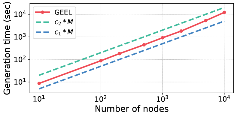
Figure 4: Infer. time on various graph sizes.

Table 2: Inference time (sec) to generate one graph.

Method	Type	Enzymes	Planar	Grid
GRAN	Auto. Reg.	00.24	00.66	01.39
BiGG	Auto. Reg.	02.70	00.61	03.58
GDSS	Diffusion	15.21	15.25	30.89
DiGress	Diffusion	08.82	12.09	32.29
GEEL (ours)	Auto. Reg.	00.12	00.25	01.11

Scalability analysis. Next, we empirically validate the time complexity of our model. We first verify if the actual inference time aligns well with the theoretical $O(M)$ curve. To this end, we generated Grid graphs with varying numbers of nodes: [10, 100, 200, 500, 1k, 2k, 5k, 10k]. The results shown in Figure 4 indicate an alignment between the actual inference time and the ideal curve.

Table 3: Vocabulary and representation sizes. The vocabulary size is $B^{2}$ and the representation size is $M$ where $B$ is bandwidth, $N$ is the number of nodes, and $M$ is the number of edges.

Dataset	Vocab. size	Rep. size	$N^{2}$
Planar	676	181	4096
Lobster	2401	99	9604
Enzymes	361	149	15625
SBM	12321	1129	34969
Ego	58081	1071	$>10^{6}$
Grid	361	684	467856
Proteins	62500	1575	$>10^{6}$
3D point cloud	111556	10886	$>10^{7}$

Then we conduct further experiments to compare the inference time of our model with that of other baselines. Note that we used the same computational resource for all models and other experimental details are in Appendix B. The results presented in Table 2 represent the time required to generate a single sample. Notably, our model shows a shorter inference time owing to the compactness of our representation, GEEL, even compared to other scalable graph generative models (Liao et al., 2019; Dai et al., 2020). This evidence underscores the scalability advantages of our GEEL.

In addition, we provide the reduced representation and vocabulary sizes in Table 3. Note that the vocabulary size of the original edge list and the representation size of the adjacency matrix are both $N^{2}$. We can observe that GEEL is efficient in both sizes.

4.2 Molecular graph generation

Table 4: Molecular graph generation performance of the QM9 and ZINC datasets. The baseline results are from prior works (Jo et al., 2022; Ahn et al., 2022). The best results of molecule-specific generative models and domain-agnostic generative models are both highlighted in bold.

	QM9						ZINC250k
Method	Val. (%)	NSPDK	FCD	Scaf.	SNN	Frag.	Val. (%)	NSPDK	FCD	Scaf.	SNN	Frag.
	$(\uparrow)$	$(\downarrow)$	$(\downarrow)$	$(\uparrow)$	$(\uparrow)$	$(\uparrow)$	$(\uparrow)$	$(\downarrow)$	$(\downarrow)$	$(\uparrow)$	$(\uparrow)$	$(\uparrow)$
Molecule-specific generative models
CharRNN	99.57	0.0003	0.087	0.9313	0.5162	0.9887	96.95	0.0003	0.474	0.4024	0.3965	0.9988
CG-VAE	100.0	-	1.852	0.6628	0.3940	0.9484	100.0	-	11.335	0.2411	0.2656	0.8118
MoFlow	91.36	0.0169	4.467	0.1447	0.3152	0.6991	63.11	0.0455	20.931	0.0133	0.2352	0.7508
STGG	100.0	-	0.585	0.9416	0.9998	0.9984	100.0	-	0.278	0.7192	0.4664	0.9932
Domain-agnostic graph generative models
EDP-GNN	47.52	0.0046	2.680	0.3270	0.5265	0.8313	63.11	0.0485	16.737	0.0000	0.0815	0.0000
GraphAF	74.43	0.0207	5.625	0.3046	0.4040	0.8319	68.47	0.0442	v16.023	0.0672	0.2422	0.5348
GraphDF	93.88	0.0636	10.928	0.0978	0.2948	0.4370	90.61	0.1770	33.546	0.0000	0.1722	0.2049
GDSS	95.72	0.0033	2.900	0.6983	0.3951	0.9224	97.01	0.0195	14.656	0.0467	0.2789	0.8138
DiGress	98.19	0.0003	0.095	0.9353	0.5263	0.0023	94.99	0.0021	3.482	0.4163	0.3457	0.9679
DruM	99.69	0.0002	0.108	0.9449	0.5272	0.9867	98.65	0.0015	2.257	0.5299	0.3650	0.9777
GraphARM	90.25	0.0020	1.220	-	-	-	88.23	0.0550	16.260	-	-	-
GEEL (ours)	100.0	0.0002	0.089	0.9386	0.5161	0.9891	99.31	0.0068	0.401	0.5565	0.4473	0.992

Experimental setup. We use two molecular datasets: QM9 (Ramakrishnan et al., 2014) and ZINC250k (Irwin et al., 2012). Following the previous work (Jo et al., 2022), we evaluate 10,000 generated molecules using six metrics: (a) the ratio of valid molecules without correction (Val.), (b) neighborhood subgraph pairwise distance kernel (NSPDK), (c) Frechet ChemNet Distance (FCD) (Preuer et al., 2018), (d) scaffold similarity (Scaf.), (e) similarity to the nearest neighbor (SNN), and (f) fragment similarity (Frag.). We use the same split with Jo et al. (2022) for a fair comparison. Note that in contrast to other general graph generation methods, our approach uniquely facilitates the direct representation of ions by employing them as a node type. We provide details in Appendix A.

Baselines. We compare GEEL with seven general deep graph generative models: EDP-GNN (Niu et al., 2020), GraphAF (Shi et al., 2020), GraphDF (Luo et al., 2021), GDSS (Jo et al., 2022), DiGress (Vignac et al., 2022), DruM (Jo et al., 2023), and GraphARM (Kong et al., 2023). In addition, for further comparison, we also compare GEEL with four molecule-specific generative models: CharRNN (Segler et al., 2018), CG-VAE (Jin et al., 2020), MoFlow (Zang & Wang, 2020), and STGG (Ahn et al., 2022). We provide a detailed implementation description in Appendix B.

Results. The experimental results are reported in Table 4. We observe that our GEEL shows superior results to domain-agnostic graph generative models and competitive results with molecule-specific generative models. In particular, for the QM9 dataset, we observe that our GEEL shows superior results on FCD and Scaffold scores even compared to the molecule-specific models. We also provide the visualization of generated molecules in Appendix D.

4.3 Ablation studies

Table 5: Average MMD results for different model architectures.

Backbone	Planar	Enzymes	Grid
LSTM	0.002	0.009	0.000
Transformer	0.003	0.008	0.000

Table 6: Average MMD for different representations. We adopted LSTM as a model architecture and OOM denotes out-of-memory error.

Representation	Repr.	Vocab.	Com.-small	Grid	Point
Flattened adj.	$N^{2}$	$2$	0.029	OOM	OOM
Edge list	$M$	$N^{2}$	0.010	0.000	OOM
Edge list + intra gap	$M$	$NB$	0.013	0.000	OOM
GEEL (ours)	$M$	$B^{2}$	0.016	0.000	0.044

Different model architectures. Here, we discuss the results of generating GEEL with Transformers (Vaswani et al., 2017). We evaluate four datasets: Planar, Lobster, Enzymes, and Grid, employing three MMD metrics for assessment. As presented in Table 5, LSTM shows competitive results to Transformers. Notably, LSTM achieves this performance with significantly reduced computational cost, having a linear complexity of $O(n)$, in contrast to the quadratic complexity $O(n^{2})$ of Transformers, where $n$ represents the sequence length.

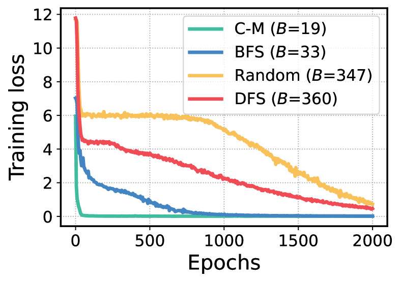
Figure 5: Training curve with various node orderings.

Different representations. We discuss the results of generating graphs with various representations here. We compare our GEEL with three alternative representations: flattened adjacency matrix, the edge list, and the edge list with intra-edge gap. The edge list is the edge list with traditional edge encoding (without any gap encoding) and the last one is an edge list wherein the target node of each edge is substituted by its intra-edge gap. Note that the edge lists are sorted in the same way we sort the edge list, as explained in Section 3.1. The comparative results are in Table 6. We can observe that GEEL effectively reduces the vocabulary size compared to other representations. This enables the generation of large-scale graphs, such as 3D point clouds, without memory constraints.

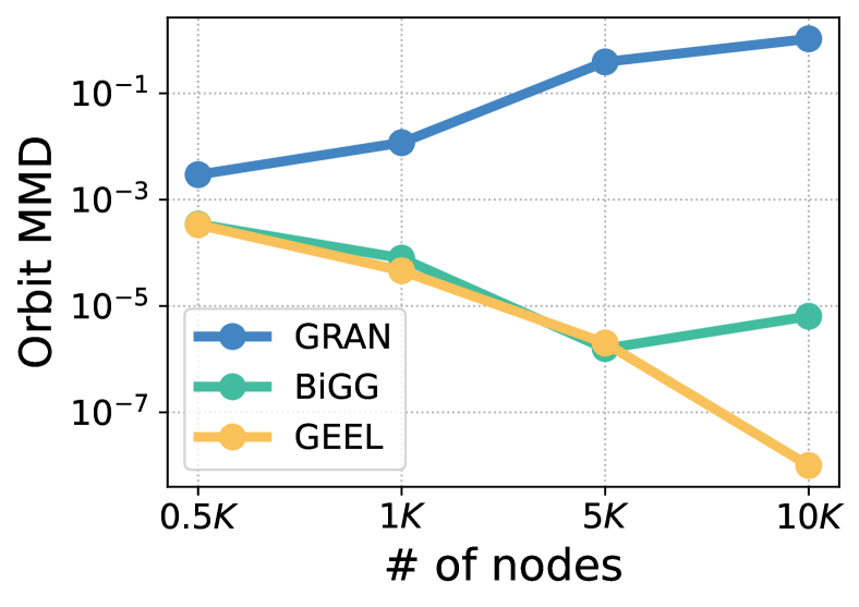
Figure 6: Orbit MMD with various graph sizes.

Different node orderings. We here assess the effect of node ordering on graph generation. We compare our C-M ordering to BFS, DFS, and random ordering using the Grid dataset. As illustrated in Figure 5, the C-M ordering outperforms others with faster convergence of training loss. Notably, the BFS also shows competitive loss convergence with C-M as it mitigates the burden of long-term dependency. Specifically, both C-M and BFS orderings position edges related to the same node more closely than other baselines. These results highlight the effectiveness of C-M ordering on bandwidth reduction and generating high-quality graphs. Note that the MMD performance with any ordering eventually converges to the same levels of MMD as explained in Appendix H.

Quality with various graph sizes. We also evaluate the generated graph quality with respect to the graph size. Following a prior work (Dai et al., 2020), we conduct experiments on grid data with {0.5k, 1k, 5k, 10k} nodes and reported orbit MMD. The results are in Figure 6 and we can see GEEL preserves high quality on large-scale graphs with up to 10k nodes.

5 Conclusion

In this work, we introduce GEEL, an edge list-based graph representation that is both simple and scalable. By combining GEEL with an LSTM, our graph generative model achieves an $O(M)$ complexity, showing a significant enhancement in generation quality and scalability over prior graph generative models.

Reproducibility All experimental code related to this paper is provided in the attached zip file. Detailed insights regarding the experiments, encompassing dataset and model specifics, are available in Section 4. For intricate details like hyperparameter search, consult Appendix A. In addition, the reproduced dataset for each baseline is in Appendix B.

Appendix A Experimental Details

In this section, we provide the details of the experiments.

A.1 General graph generation

Table 7: Hyperparameters of GEEL in general graph generation.

	Planar	Lobster	Enzymes	SBM	Ego	Grid	Proteins	3D point cloud
Learning rate	0.001	0.0001	0.0005	0.0001	0.0001	0.001	0.0001	0.0012
Batch size	128	64	128	8	8	64	8	4

Table 8: Default hyperparameters of GEEL.

Input dropout rate	Dim. of token embedding	Num. of layers
0.1	512	3

We used the same split with GDSS (Jo et al., 2022) for Enzymes and Grid datasets, with DiGress (Vignac et al., 2022) for Planar and SBM datasets, with BiGG (Dai et al., 2020) for Lobster, Proteins, and 3D point cloud datasets, and with GraphRNN (You et al., 2018) for ego dataset. We perform the hyperparameter search to choose the best learning rate in {0.0001, 0.0005, 0.001, and 0.0012}. We select the model with the best MMD with the lowest average of three graph statistics: degree, clustering coefficient, and 4-orbit count. In addition, we report the means of 5 different runs. It is notable that GEEL samples a C-M ordering for a graph at each training step (instead of fixing a unique ordering per graph). We found this to improve novelty without any decrease in performance and changing the hyper-parameters. We provide the best learning rates in Table 7 and other default hyperparameters that we have not tuned in Table 8.

A.2 Molecular graph generation

We used the same split with GDSS (Jo et al., 2022) for a fair evaluation. Following general graph generation, we perform the hyperparameter search to choose the best learning rate in {0.0001, 0.001} and select the model with the best FCD score. The best learning rates are 0.001 for both QM9 and ZINC datasets and other default hyperparameters are in Table 8 which is the same as the general graph generation.

For ion tokenization, we used 13 node tokens for QM9: [C-], [CH-], [C], [F], [N+], [N-], [NH+], [NH2+], [NH3+], [NH], [N], [O-], [O]. In addition, we used 29 tokens for ZINC: [Br], [CH-], [CH2-], [CH], [C], [Cl], [F], [I], [N+], [N-], [NH+], [NH-], [NH2+], [NH3+], [NH], [N], [O+], [O-], [OH+], [O], [P+], [PH+], [PH2], [PH], [P], [S+], [S-], [SH+], [S].

Appendix B Implementation Details

B.1 Computing resources

We used Pytorch (Paszke et al., 2019) to implement GEEL and trained the LSTM (Hochreiter & Schmidhuber, 1997) models on GeForce RTX 3090 GPU. Note that we used A100-40GB for the 3D point cloud dataset. In addition, due to the CUDA compatibility issue of BiGG (Dai et al., 2020), we used GeForce GTX 1080 Ti GPU and 40 CPU cores for all models for inference time evaluation in Figure 1(c) and Table 2.

B.2 Details for baseline implementation

Table 9: Reproduced dataset for each baselines.

	Planar	Lobster	Enzymes	SBM	Ego	Grid	Proteins	3D point cloud
GRAN	-	-	$\checkmark$	-	$\checkmark$	-	-	-
GraphGen	$\checkmark$	$\checkmark$	$\checkmark$	$\checkmark$	$\checkmark$	$\checkmark$	$\checkmark$	$\checkmark$
BiGG	$\checkmark$	-	$\checkmark$	$\checkmark$	$\checkmark$	-	-	-
GDSS	$\checkmark$	$\checkmark$	-	$\checkmark$	$\checkmark$	-	$\checkmark$	$\checkmark$
DiGress	-	$\checkmark$	$\checkmark$	-	$\checkmark$	$\checkmark$	$\checkmark$	$\checkmark$

General graph generation. The baseline results from prior works are as follows. We reproduced GRAN (Liao et al., 2019), GraphGen (Goyal et al., 2020), DiGress (Vignac et al., 2022), GDSS (Jo et al., 2022) and BiGG (Dai et al., 2020) for the datasets that are not reported in the original paper using their open-source codes. The reproduced datasets are explained in Table 9. The other results for GraphVAE (Simonovsky & Komodakis, 2018), GNF (Liu et al., 2019), EDP-GNN (Niu et al., 2020), GraphAF (Shi et al., 2020), GraphDF (Luo et al., 2021), and GDSS (Jo et al., 2022) are obtained from GDSS, while the results for GRAN (Liao et al., 2019), GraphRNN (You et al., 2018), and BiGG (Dai et al., 2020) are from BiGG and SPECTRE (Martinkus et al., 2022). Finally, the remaining results for SPECTRE and GDSM (Luo et al., 2022) are derived from their respective paper. We used original hyperparameters when the original work provided them.

Molecular graph generation. The baseline results from prior works are as follows. The results for five domain-agnostic graph generative models: EDP-GNN (Niu et al., 2020), GraphAF (Shi et al., 2020), GraphDF (Luo et al., 2021), GDSS (Jo et al., 2022), DruM (Jo et al., 2023) are from DruM, and the GraphARM (Kong et al., 2023) result is extracted from the corresponding paper. Moreover, we reproduced DiGress (Vignac et al., 2022) using their open-source codes.

In addition, for molecule generative models, the result of MoFlow (Zang & Wang, 2020) is from DruM, the results of CG-VAE (Jin et al., 2020) and STGG (Ahn et al., 2022) is from STGG. Furthermore, we reproduced CharRNN (Segler et al., 2018).

B.3 Details for inference time analysis

We conducted the inference time analysis using the same GeForce GTS 1080 Ti GPU for all models. The batch size is 10 and the inference time to generate a single is simply computed by dividing the total inference time by the batch size.

B.4 Details for the implementation

We adapted node ordering code from (Diamant et al., 2023), evaluation scheme from (Jo et al., 2022; Martinkus et al., 2022), and NSPDK computation from (Goyal et al., 2020).

Appendix C Graph statistics of datasets

C.1 General graphs

Table 10: Statstics of general datasets.

Dataset	# of graphs	# of nodes	Max. $B$	Max. # of edges
Planar	200	$|V|=64$	26	181
Lobster	100	$10\leq|V|\leq 100$	49	99
Enzymes	587	$10\leq|V|\leq 125$	19	149
SBM	200	$31\leq|V|\leq 187$	111	1129
Ego	757	$50\leq|V|\leq 399$	241	1071
Grid	100	$100\leq|V|\leq 400$	19	684
Proteins	918	$13\leq|V|\leq 1575$	125	1575
3D point cloud	41	$8\leq|V|\leq 5037$	167	10886

Table 11: Standard deviation of MMD in training dataset.

Planar			Lobster			Enzymes			SBM
Deg.	Clus.	Orb.	Deg.	Clus.	Orb.	Deg.	Clus.	Orb.	Deg.	Clus.	Orb.
0.000	0.001	0.000	0.003	0.000	0.006	0.001	0.003	0.002	0.008	0.002	0.017

(a) Small graphs ($|V|_{\max}\leq 187$)

Ego			Grid			Proteins			3D point cloud
Deg.	Clus.	Orb.	Deg.	Clus.	Orb.	Deg.	Clus.	Orb.	Deg.	Clus.	Orb.
0.005	0.001	0.004	0.000	0.000	0.000	0.001	0.002	0.001	0.04	0.062	0.017

(b) Large graphs ($399\leq|V|_{\max}\leq 5037$)

The statistics of general graphs are summarized in Table 10. It is notable that the bandwidths are relatively low compared to the number of nodes for real-world graphs, which enables the reduction of the vocabulary size of GEEL. In addition, we provide the standard deviations of MMD of training graphs that we used as a criterion to verify comparability in Table 11.

C.2 Molecular graphs

Table 12: Statstics of molecular datasets: QM9 and ZINC250k.

Dataset	# of graphs	# of nodes	Max. $B$	Max. # of edges	# of node types	# of edge types
QM9	133,885	$1\leq|V|\leq 9$	5	13	13	4
ZINC250k	249,455	$6\leq|V|\leq 38$	10	45	29	4

The statistics of molecular graphs are summarized in Table 12. Note that the # of node types indicate the number of ionized node type tokens as explained in Appendix A.

Appendix D Generated samples

D.1 General graph generation

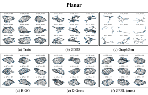
Figure 7: Visualization of the graphs from the Planar dataset and the generated graphs.

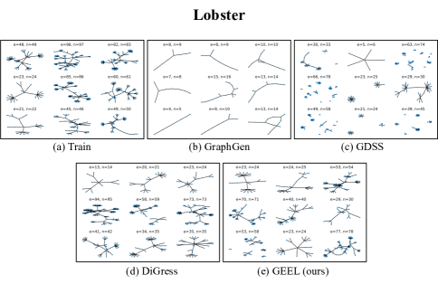
Figure 8: Visualization of the graphs from the Lobster dataset and the generated graphs.

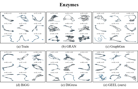
Figure 9: Visualization of the graphs from the Enzymes dataset and the generated graphs.

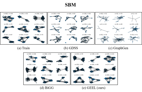
Figure 10: Visualization of the graphs from the SBM dataset and the generated graphs.

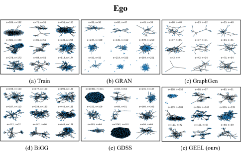
Figure 11: Visualization of the graphs from the Ego dataset and the generated graphs.

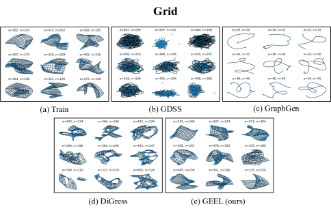
Figure 12: Visualization of the graphs from the Grid dataset and the generated graphs.

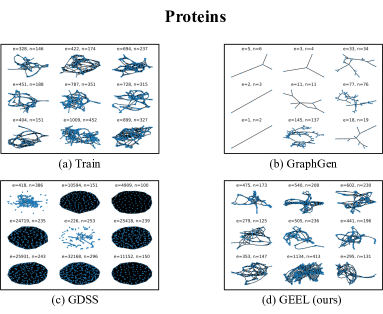
Figure 13: Visualization of the graphs from the Proteins dataset and the generated graphs.

We present visualizations of graphs from the training dataset and generated samples from GRAN, GraphGen, BiGG, GDSS, DiGress, and GEEL in Figure 7, Figure 8, Figure 9, Figure 10, Figure 11, Figure 12, and Figure 13. Note that we only provide the visualization that we have reproduced, which is detailed in Appendix B. We additionally give the number of nodes and edges of each graph, where $n$ denotes the number of nodes and $e$ denotes the number of edges.

D.2 Molecular graph genereation

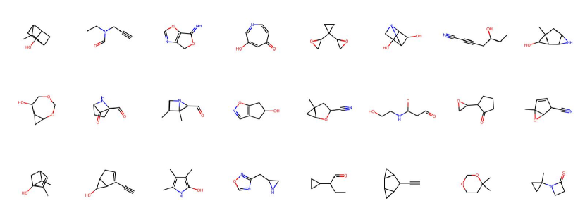
Figure 14: Visualization of the molecules generated from the QM9 dataset.

Figure 15: Visualization of the molecules generated from the ZINC250k dataset.

We provide visualizations of generated molecules using GEEL in Figure 14 and Figure 15.

Appendix E Additional Experimental Results

E.1 General graph generation

Table 13: General graph generation on small graphs ($|V|_{\max}\leq 20$)

	Ego-small			Community-small
	$4\leq|V|\leq 18$			$12\leq|V|\leq 20$
Method	Deg.	Clus.	Orb.	Deg.	Clus.	Orb.
Training	0.025	0.035	0.012	0.020	0.044	0.003
GraphVAE	0.130	0.170	0.050	0.350	0.980	0.540
GraphRNN	0.090	0.220	0.003	0.080	0.120	0.040
GRAN	0.009	0.038	0.009	0.005	0.142	0.090
GNF	0.030	0.100	0.001	0.200	0.200	0.110
EDP-GNN	0.052	0.093	0.007	0.053	0.144	0.026
GraphGen	0.085	0.102	0.425	0.075	0.065	0.014
GraphAF	0.030	0.110	0.001	0.180	0.200	0.020
GraphDF	0.040	0.130	0.010	0.060	0.120	0.030
BiGG	0.013	0.030	0.005	0.004	0.005	0.000
GDSS	0.021	0.024	0.007	0.045	0.086	0.007
DiGress	0.021	0.026	0.024	0.012	0.025	0.002
GDSM	-	-	-	0.011	0.015	0.001
GraphARM	0.019	0.017	0.010	0.034	0.082	0.004
SwinGNN	0.000	0.021	0.004	0.003	0.051	0.004
GEEL (ours)	0.020	0.035	0.012	0.020	0.022	0.006

We provide general graph generation results for smaller graph datasets: Ego-small and Community-small. The Ego-small dataset consists of 300 small ego graphs from larger Citeseer network (Sen et al., 2008) and Community-small dataset consists of 100 randomly generated community graphs. We used the same split with GDSS (Jo et al., 2022) and the results are reported in Table 13.

E.2 Molecular graph generation

We provide molecular graph generation results for MOSES benchmark (Polykovskiy et al., 2020) in Table 14.

Table 14: Molecular graph generation performance of MOSES dataset. The baseline results are from prior works (Polykovskiy et al., 2020; Ahn et al., 2022). The best results are highlighted in bold and the second best are underlined.

	MOSES
Method	Validity (%) $\uparrow$	NSPDK $\downarrow$	FCD $\downarrow$	Scaf. $\uparrow$	SNN $\uparrow$	Frag. $\uparrow$
Molecule generative models
CharRNN	97.48	-	0.0732	0.9242	0.6015	0.9998
JT-VAE	100.00	-	0.3954	0.8964	0.5477	0.9965
STGG	100.00	-	0.0680	0.9416	0.6359	0.9998
Domain-agnostic graph generative models
DiGress	100.00	0.0005	0.6788	0.8653	0.5488	0.9988
GEEL (Ours)	99.99	0.0001	0.1603	0.8622	0.6310	0.9996

Appendix F Additional metrics

F.1 General graph generation

We provide three additional metrics: validity, uniqueness, and novelty scores for general graph generation in Table 15. GEEL achieves from 30% to 90% novelty, which is better than autoregressive models like GRAN and BiGG, but lower than the diffusion-based graph generative models. This is partially due to the inherent trade-off between novelty and the capability of generative models to faithfully learn the data distribution. OOM indicates out-of-memory and N.A. for BwR indicates that the generated samples are all invalid.

Table 15: The results of general graph generation including validity, uniqueness, and novelty. The baseline results are from prior works (Martinkus et al., 2022; Vignac et al., 2022) or obtained by running the open-source codes.

	Planar						Lobster
	$|V|=64$						$10\leq|V|\leq 100$
Method	Deg. $(\downarrow)$	Clu. $(\downarrow)$	Orb. $(\downarrow)$	Val. $(\uparrow)$	Uniq. $(\uparrow)$	Nov. $(\uparrow)$	Deg. $(\downarrow)$	Clu. $(\downarrow)$	Orb. $(\downarrow)$	Val. $(\uparrow)$	Uniq. $(\uparrow)$	Nov. $(\uparrow)$
GraphRNN	0.005	0.278	1.254	0.0	100.0	100.0	0.000	0.000	0.000	-	-	-
GRAN	0.001	0.043	0.001	97.5	85.0	2.5	0.038	0.000	0.001	-	-	-
SPECTRE	0.001	0.079	0.001	25.0	100.0	100.0	-	-	-	-	-	-
BiGG	0.002	0.004	0.000	100.0	85.0	0.0	0.000	0.000	0.000	-	-	-
GDSS	0.250	0.393	0.587	0.0	100.0	100.0	0.117	0.002	0.149	18.2	100.0	100.0
DiGress	0.000	0.002	0.008	85.0	100.0	100.0	0.021	0.000	0.004	54.5	100.0	100.0
BwR + GraphRNN	0.609	0.542	0.097	52.5	95.0	100.0	0.316	0.000	0.247	100.0	63.6	100.0
BwR + Graphite	0.971	0.562	0.636	3.4	100.0	100.0	0.076	1.075	0.060	0.0	100.0	100.0
BwR + EDP-GNN	1.127	1.032	0.066	0.0	100.0	100.0	0.237	0.062	0.166	0.0	100.0	100.0
GEEL (ours)	0.001	0.010	0.001	82.5	97.5	27.5	0.002	0.000	0.001	72.7	100	72.7

	Enzymes					SBM
	$10\leq|V|\leq 125$					$31\leq|V|\leq 187$
Method	Deg. $(\downarrow)$	Clu. $(\downarrow)$	Orb. $(\downarrow)$	Uniq. $(\uparrow)$	Nov. $(\uparrow)$	Deg. $(\downarrow)$	Clu. $(\downarrow)$	Orb. $(\downarrow)$	Uniq. $(\uparrow)$	Nov. $(\uparrow)$
GraphRNN	0.017	0.062	0.046	-	-	0.006	0.058	0.079	100.0	100.0
GRAN	0.023	0.031	0.169	100.0	94.9	0.011	0.055	0.054	100.0	100.0
SPECTRE	-	-	-	-	-	0.002	0.052	0.041	100.0	100.0
BiGG	0.010	0.018	0.011	78.8	4.2	0.029	0.003	0.036	92.5	10.0
GDSS	0.026	0.061	0.009	-	-	0.496	0.456	0.717	100.0	100.0
DiGress	0.011	0.039	0.010	100.0	99.2	0.006	0.051	0.058	100.0	100.0
BwR + GraphRNN	0.021	0.095	0.025	97.5	100.0	N.A.	N.A.	N.A.	N.A.	N.A.
BwR + Graphite	0.213	0.270	0.056	100.0	100.0	1.305	1.341	1.056	100.0	100.0
BwR + EDP-GNN	0.253	0.118	0.168	100.0	100.0	0.657	1.679	0.275	100.0	100.0
GEEL (ours)	0.005	0.018	0.006	100.0	94.9	0.025	0.003	0.026	95.0	42.5

	Ego					Proteins
	$50\leq|V|\leq 399$					$13\leq|V|\leq 1575$
Method	Deg. $(\downarrow)$	Clu. $(\downarrow)$	Orb. $(\downarrow)$	Uniq. $(\uparrow)$	Nov. $(\uparrow)$	Deg. $(\downarrow)$	Clu. $(\downarrow)$	Orb. $(\downarrow)$	Uniq. $(\uparrow)$	Nov. $(\uparrow)$
GraphRNN	0.117	0.615	0.043	-	-	0.011	0.140	0.880	100.0	100.0
GRAN	0.026	0.342	0.254	-	-	0.002	0.049	0.130	100.0	100.0
SPECTRE	-	-	-	-	-	0.013	0.047	0.029	100.0	100.0
BiGG	0.010	0.017	0.012	89.5	57.2	0.001	0.026	0.023	-	-
GDSS	0.393	0.873	0.209	100.0	100.0	0.703	1.444	0.410	99.5	100.0
DiGress	0.063	0.031	0.024	100.0	100.0	OOM	OOM	OOM	OOM	OOM
BwR + GraphRNN	N.A.	N.A.	N.A.	N.A.	N.A.	0.092	0.229	0.489	-	-
BwR + Graphite	0.229	0.123	0.054	100.0	100.0	0.239	0.245	0.492	-	-
BwR + EDP-GNN	OOM	OOM	OOM	OOM	OOM	0.184	0.208	0.738	-	-
GEEL (ours)	0.053	0.017	0.016	89.4	62.8	0.003	0.005	0.003	93.7	88.9

	3d point cloud
	$8\leq|V|\leq 5037$
Method	Deg. $(\downarrow)$	Clu. $(\downarrow)$	Orb. $(\downarrow)$	Uniq. $(\uparrow)$	Nov. $(\uparrow)$
GraphVAE	OOM	OOM	OOM	OOM	OOM
GraphRNN	OOM	OOM	OOM	OOM	OOM
GRAN	0.018	0.510	0.210	-	-
BiGG	0.003	0.210	0.007	-	-
GDSS	OOM	OOM	OOM	OOM	OOM
DiGress	OOM	OOM	OOM	OOM	OOM
BwR + GraphRNN	1.820	1.295	0.869	100.0	100.0
BwR + Graphite	OOM	OOM	OOM	OOM	OOM
BwR + EDP-GNN	OOM	OOM	OOM	OOM	OOM
GEEL (ours)	0.002	0.081	0.020	100.0	80.0

F.2 Molecular graph generation

We also provide the uniqueness and novelty scores for QM9 and ZINC in Table 16. We can observe that our GEEL shows competitive novelty and uniqueness compared to the baselines. Notably, the models make a tradeoff between the quality (e.g., NSPDK and FCD) and novelty of the generated graph since the graph generative models that faithfully learn the distribution put a high likelihood on the training dataset. In particular, the tradeoff is more significant in QM9 due to the large dataset size (134k) compared to the relatively small search space (molecular graphs with only up to nine heavy atoms).

Table 16: Molecular graph generation performance of the QM9 and ZINC datasets including novelty and uniqueness. The baseline results are from prior works (Jo et al., 2023; Ahn et al., 2022). The best results of molecule generative models and domain-agnostic generative models are both highlighted in bold.

	QM9
Method	Validity (%) $(\uparrow)$	NSPDK $(\downarrow)$	FCD $(\downarrow)$	Scaf. $(\uparrow)$	SNN $(\uparrow)$	Frag. $(\uparrow)$	Unique. (%) $(\uparrow)$	Novelty (%) $(\uparrow)$
Molecule-specific generative models
CharRNN	99.57	0.0003	0.087	0.9313	0.5162	0.9887	-	-
CG-VAE	100.0	-	1.852	0.6628	0.3940	0.9484	-	-
MoFlow	91.36	0.0169	4.467	0.1447	0.3152	0.6991	98.65	94.72
STGG	100.0	-	0.585	0.9416	0.9998	0.9984	96.76	72.73
Domain-agnostic graph generative models
EDP-GNN	47.52	0.0046	2.680	0.3270	0.5265	0.8313	99.25	86.58
GraphAF	74.43	0.0207	5.625	0.3046	0.4040	0.8319	88.64	86.59
GraphDF	93.88	0.0636	10.928	0.0978	0.2948	0.4370	98.58	98.54
GDSS	95.72	0.0033	2.900	0.6983	0.3951	0.9224	98.46	86.27
DiGress	98.19	0.0003	0.095	0.9353	0.5263	0.0023	96.67	25.58
DruM	99.69	0.0002	0.108	0.9449	0.5272	0.9867	96.90	24.15
GraphARM	90.25	0.0020	1.220	-	-	-	-	-
GEEL (ours)	100.0	0.0002	0.089	0.9386	0.5161	0.9891	96.08	22.30

	ZINC
Method	Validity (%) $(\uparrow)$	NSPDK $(\downarrow)$	FCD $(\downarrow)$	Scaf. $(\uparrow)$	SNN $(\uparrow)$	Frag. $(\uparrow)$	Unique. (%) $(\uparrow)$	Novelty (%) $(\uparrow)$
Molecule-specific generative models
CharRNN	6.95	0.0003	0.474	0.4024	0.3965	0.9988	-	-
CG-VAE	100.0	-	11.335	0.2411	0.2656	0.8118	-	-
MoFlow	91.36	0.0169	4.467	0.1447	0.3152	0.6991	99.99	100.00
STGG	63.11	0.0455	20.931	0.0133	0.2352	0.7508	99.99	99.89
Domain-agnostic graph generative models
EDP-GNN	63.11	0.0485	16.737	0.0000	0.0815	0.0000	99.79	100.00
GraphAF	68.47	0.0442	16.023	0.0672	0.2422	0.5348	98.64	99.99
GraphDF	90.61	0.1770	33.546	0.0000	0.1722	0.2049	99.63	100.00
GDSS	97.01	0.0195	14.656	0.0467	0.2789	0.8138	99.64	100.00
DiGress	94.99	0.0021	3.482	0.4163	0.3457	0.9679	99.97	99.99
DruM	98.65	0.0015	2.257	0.5299	0.3650	0.9777	99.97	99.98
GraphARM	88.23	0.0550	16.260	-	-	-	-	-
GEEL (ours)	99.31	0.0068	0.401	0.5565	0.4473	0.992	99.97	99.89

Appendix G Discussion

G.1 Limitation

In this section, we discuss the limitations of our GEEL. The limitation of GEEL is two-fold: (1) unable to generate graphs with unseen tokens and (2) dependency on the bandwidth. Since GEEL is based on the vocabulary with gap-encoded edge tokens, the model cannot generate the graphs with unseen tokens, i.e., the graphs with larger bandwidth than the training graphs. Nonetheless, we believe the generalization capability of our GEEL is strong enough in practice. In all the experiments, we verified that our vocabulary obtained from the training dataset entirely captures the vocabulary required for generating graphs in the test dataset.

Another limitation is the dependency on the bandwidth, i.e., the vocabulary size of GEEL is the square of the bandwidth. It is true that the vocabulary size of GEEL is highly dependent on the bandwidth. However, most of the real-world large-scale graphs have small bandwidths as described in Table 12 so $B$ being as large as $N$ is rare in practice. Additionally, for larger graphs with $B\approx N$, one could consider (a) decomposing the graph into subgraphs with small bandwidth and (b) separately generating the subgraphs using GEEL. This would be an interesting future avenue of research.

G.2 Comparison to BwR

Here, we compare our GEEL to BwR (Diamant et al., 2023). Overall, Our work proposes a new edge list representation with the vocabulary size of $B^{2}$ with gap encoding. Although we promote reducing the bandwidth $B$ using the C-M ordering, as proposed by BwR, our key idea, the gap encoding edge list is orthogonal to BwR. Our analysis of $B^{2}$ vocabulary size simply follows the definition of graph bandwidth. Moreover, one could also choose any bandwidth minimization algorithm (e.g., BFS ordering used in GraphRNN) to reduce the vocabulary size $B^{2}$.

In detail, we compare our GEEL to three variants of BwR. First, BwR+GraphRNN iteratively adds a node to the graph by adding the neighbors independently at once using a multivariate Bernoulli distribution. This ignores the dependencies between adjacent edges, which our GEEL captures via the edge-wise updates. Next, BwR+Graphite is a VAE-based generative model that generates the whole graph in a one-shot manner. This also does not consider the edge dependencies during generation, while our GEEL does. Finally, BwR+EDP-GNN is a diffusion-based model that generates the continuous relaxation of the adjacency matrix. It requires the generative model to learn the complicated reverse diffusion process, which results in underfitting of the model. This issue is especially significant since the BwR+EDP-GNN uses a small number of 200 diffusion steps.

Appendix H Additional results for ablation study

	Deg.	Clus.	Orb.
BFS	0.000	0.000	0.000
DFS	0.000	0.000	0.000
Random	0.000	0.000	0.000
C-M	0.000	0.000	0.000

Table 17: MMD on different node orderings

We provide the MMD performance of the ablation study on different orderings of Section 4.3 in Table 17. We can observe that the generation with any ordering eventually converges to the same levels of MMD.

References

- Ahn et al. (2022) Sungsoo Ahn, Binghong Chen, Tianzhe Wang, and Le Song. Spanning tree-based graph generation for molecules. In International Conference on Learning Representations, 2022. URL https://openreview.net/forum?id=w60btE_8T2m.
- Bacciu & Podda (2021) Davide Bacciu and Marco Podda. Graphgen-redux: A fast and lightweight recurrent model for labeled graph generation. In 2021 International Joint Conference on Neural Networks (IJCNN), pp. 1–8. IEEE, 2021.
- Chinn et al. (1982) Phyllis Z Chinn, Jarmila Chvátalová, Alexander K Dewdney, and Norman E Gibbs. The bandwidth problem for graphs and matrices—a survey. Journal of Graph Theory, 6(3):223–254, 1982.
- Collins (2003) Michael Collins. Head-driven statistical models for natural language parsing. Computational linguistics, 29(4):589–637, 2003.
- Cuthill & McKee (1969) Elizabeth Cuthill and James McKee. Reducing the bandwidth of sparse symmetric matrices. In Proceedings of the 1969 24th national conference, pp. 157–172, 1969.
- Dai et al. (2020) Hanjun Dai, Azade Nazi, Yujia Li, Bo Dai, and Dale Schuurmans. Scalable deep generative modeling for sparse graphs. In International conference on machine learning, pp. 2302–2312. PMLR, 2020.
- Diamant et al. (2023) Nathaniel Lee Diamant, Alex M Tseng, Kangway V Chuang, Tommaso Biancalani, and Gabriele Scalia. Improving graph generation by restricting graph bandwidth. In International Conference on Machine Learning, pp. 7939–7959. PMLR, 2023.
- Goyal et al. (2020) Nikhil Goyal, Harsh Vardhan Jain, and Sayan Ranu. Graphgen: a scalable approach to domain-agnostic labeled graph generation. In Proceedings of The Web Conference 2020, pp. 1253–1263, 2020.
- Grover et al. (2019) Aditya Grover, Aaron Zweig, and Stefano Ermon. Graphite: Iterative generative modeling of graphs. In International conference on machine learning, pp. 2434–2444. PMLR, 2019.
- Guo et al. (2022) Minghao Guo, Veronika Thost, Beichen Li, Payel Das, Jie Chen, and Wojciech Matusik. Data-efficient graph grammar learning for molecular generation. arXiv preprint arXiv:2203.08031, 2022.
- Ho et al. (2020) Jonathan Ho, Ajay Jain, and Pieter Abbeel. Denoising diffusion probabilistic models. Advances in neural information processing systems, 33:6840–6851, 2020.
- Hochreiter & Schmidhuber (1997) Sepp Hochreiter and Jürgen Schmidhuber. Long short-term memory. Neural computation, 9(8):1735–1780, 1997.
- Irwin et al. (2012) John J Irwin, Teague Sterling, Michael M Mysinger, Erin S Bolstad, and Ryan G Coleman. Zinc: a free tool to discover chemistry for biology. Journal of chemical information and modeling, 52(7):1757–1768, 2012.
- Jin et al. (2018) Wengong Jin, Regina Barzilay, and Tommi Jaakkola. Junction tree variational autoencoder for molecular graph generation. In International conference on machine learning, pp. 2323–2332. PMLR, 2018.
- Jin et al. (2020) Wengong Jin, Regina Barzilay, and Tommi Jaakkola. Hierarchical generation of molecular graphs using structural motifs. In International conference on machine learning, pp. 4839–4848. PMLR, 2020.
- Jo et al. (2022) Jaehyeong Jo, Seul Lee, and Sung Ju Hwang. Score-based generative modeling of graphs via the system of stochastic differential equations. In International Conference on Machine Learning, pp. 10362–10383. PMLR, 2022.
- Jo et al. (2023) Jaehyeong Jo, Dongki Kim, and Sung Ju Hwang. Graph generation with destination-driven diffusion mixture. arXiv preprint arXiv:2302.03596, 2023.
- Kong et al. (2023) Lingkai Kong, Jiaming Cui, Haotian Sun, Yuchen Zhuang, B. Aditya Prakash, and Chao Zhang. Autoregressive diffusion model for graph generation, 2023. URL https://openreview.net/forum?id=98J48HZXxd5.
- Li et al. (2018) Yujia Li, Oriol Vinyals, Chris Dyer, Razvan Pascanu, and Peter Battaglia. Learning deep generative models of graphs. arXiv preprint arXiv:1803.03324, 2018.
- Liao et al. (2019) Renjie Liao, Yujia Li, Yang Song, Shenlong Wang, Will Hamilton, David K Duvenaud, Raquel Urtasun, and Richard Zemel. Efficient graph generation with graph recurrent attention networks. Advances in neural information processing systems, 32, 2019.
- Liu et al. (2019) Jenny Liu, Aviral Kumar, Jimmy Ba, Jamie Kiros, and Kevin Swersky. Graph normalizing flows. Advances in Neural Information Processing Systems, 32, 2019.
- Liu et al. (2021) Meng Liu, Keqiang Yan, Bora Oztekin, and Shuiwang Ji. Graphebm: Molecular graph generation with energy-based models. arXiv preprint arXiv:2102.00546, 2021.
- Luo et al. (2022) Tianze Luo, Zhanfeng Mo, and Sinno Jialin Pan. Fast graph generative model via spectral diffusion. arXiv preprint arXiv:2211.08892, 2022.
- Luo et al. (2021) Youzhi Luo, Keqiang Yan, and Shuiwang Ji. Graphdf: A discrete flow model for molecular graph generation. In International Conference on Machine Learning, pp. 7192–7203. PMLR, 2021.
- Madhawa et al. (2019) Kaushalya Madhawa, Katushiko Ishiguro, Kosuke Nakago, and Motoki Abe. Graphnvp: An invertible flow model for generating molecular graphs. arXiv preprint arXiv:1905.11600, 2019.
- Martinkus et al. (2022) Karolis Martinkus, Andreas Loukas, Nathanaël Perraudin, and Roger Wattenhofer. Spectre: Spectral conditioning helps to overcome the expressivity limits of one-shot graph generators. In International Conference on Machine Learning, pp. 15159–15179. PMLR, 2022.
- Maziarka et al. (2020) Łukasz Maziarka, Agnieszka Pocha, Jan Kaczmarczyk, Krzysztof Rataj, Tomasz Danel, and Michał Warchoł. Mol-cyclegan: a generative model for molecular optimization. Journal of Cheminformatics, 12(1):1–18, 2020.
- Niu et al. (2020) Chenhao Niu, Yang Song, Jiaming Song, Shengjia Zhao, Aditya Grover, and Stefano Ermon. Permutation invariant graph generation via score-based generative modeling. In International Conference on Artificial Intelligence and Statistics, pp. 4474–4484. PMLR, 2020.
- Paszke et al. (2019) Adam Paszke, Sam Gross, Francisco Massa, Adam Lerer, James Bradbury, Gregory Chanan, Trevor Killeen, Zeming Lin, Natalia Gimelshein, Luca Antiga, et al. Pytorch: An imperative style, high-performance deep learning library. Advances in neural information processing systems, 32, 2019.
- Polykovskiy et al. (2020) Daniil Polykovskiy, Alexander Zhebrak, Benjamin Sanchez-Lengeling, Sergey Golovanov, Oktai Tatanov, Stanislav Belyaev, Rauf Kurbanov, Aleksey Artamonov, Vladimir Aladinskiy, Mark Veselov, et al. Molecular sets (moses): a benchmarking platform for molecular generation models. Frontiers in pharmacology, 11:565644, 2020.
- Preuer et al. (2018) Kristina Preuer, Philipp Renz, Thomas Unterthiner, Sepp Hochreiter, and Gunter Klambauer. Fréchet chemnet distance: a metric for generative models for molecules in drug discovery. Journal of chemical information and modeling, 58(9):1736–1741, 2018.
- Ramakrishnan et al. (2014) Raghunathan Ramakrishnan, Pavlo O Dral, Matthias Rupp, and O Anatole Von Lilienfeld. Quantum chemistry structures and properties of 134 kilo molecules. Scientific data, 1(1):1–7, 2014.
- Schomburg et al. (2004) Ida Schomburg, Antje Chang, Christian Ebeling, Marion Gremse, Christian Heldt, Gregor Huhn, and Dietmar Schomburg. Brenda, the enzyme database: updates and major new developments. Nucleic acids research, 32(suppl_1):D431–D433, 2004.
- Segler et al. (2018) Marwin HS Segler, Thierry Kogej, Christian Tyrchan, and Mark P Waller. Generating focused molecule libraries for drug discovery with recurrent neural networks. ACS central science, 4(1):120–131, 2018.
- Sen et al. (2008) Prithviraj Sen, Galileo Namata, Mustafa Bilgic, Lise Getoor, Brian Galligher, and Tina Eliassi-Rad. Collective classification in network data. AI magazine, 29(3):93–93, 2008.
- Senger (1997) Elizabeth Senger. Polyominoes: Puzzles, patterns, problems, and packings. The Mathematics Teacher, 90(1):72, 1997.
- Shi et al. (2020) Chence Shi, Minkai Xu, Zhaocheng Zhu, Weinan Zhang, Ming Zhang, and Jian Tang. Graphaf: a flow-based autoregressive model for molecular graph generation. arXiv preprint arXiv:2001.09382, 2020.
- Simonovsky & Komodakis (2018) Martin Simonovsky and Nikos Komodakis. Graphvae: Towards generation of small graphs using variational autoencoders. In Artificial Neural Networks and Machine Learning–ICANN 2018: 27th International Conference on Artificial Neural Networks, Rhodes, Greece, October 4-7, 2018, Proceedings, Part I 27, pp. 412–422. Springer, 2018.
- Vaswani et al. (2017) Ashish Vaswani, Noam Shazeer, Niki Parmar, Jakob Uszkoreit, Llion Jones, Aidan N Gomez, Łukasz Kaiser, and Illia Polosukhin. Attention is all you need. Advances in neural information processing systems, 30, 2017.
- Vignac et al. (2022) Clement Vignac, Igor Krawczuk, Antoine Siraudin, Bohan Wang, Volkan Cevher, and Pascal Frossard. Digress: Discrete denoising diffusion for graph generation. arXiv preprint arXiv:2209.14734, 2022.
- Yan et al. (2023) Qi Yan, Zhengyang Liang, Yang Song, Renjie Liao, and Lele Wang. Swingnn: Rethinking permutation invariance in diffusion models for graph generation. arXiv preprint arXiv:2307.01646, 2023.
- You et al. (2018) Jiaxuan You, Rex Ying, Xiang Ren, William Hamilton, and Jure Leskovec. Graphrnn: Generating realistic graphs with deep auto-regressive models. In International conference on machine learning, pp. 5708–5717. PMLR, 2018.
- Zang & Wang (2020) Chengxi Zang and Fei Wang. Moflow: an invertible flow model for generating molecular graphs. In Proceedings of the 26th ACM SIGKDD International Conference on Knowledge Discovery & Data Mining, pp. 617–626, 2020.