Tracing Hyperparameter Dependencies for Model Parsing
via Learnable Graph Pooling Network

Abstract

Model Parsing defines the research task of predicting hyperparameters of the generative model (GM), given a generated image as input. Since a diverse set of hyperparameters is jointly employed by the generative model, and dependencies often exist among them, it is crucial to learn these hyperparameter dependencies for the improved model parsing performance. To explore such important dependencies, we propose a novel model parsing method called Learnable Graph Pooling Network (LGPN). Specifically, we transform model parsing into a graph node classification task, using graph nodes and edges to represent hyperparameters and their dependencies, respectively. Furthermore, LGPN incorporates a learnable pooling-unpooling mechanism tailored to model parsing, which adaptively learns hyperparameter dependencies of GMs used to generate the input image. We also extend our proposed method to CNN-generated image detection and coordinate attacks detection. Empirically, we achieve state-of-the-art results in model parsing and its extended applications, showing the effectiveness of our method. Our source code are available.

1 Introduction

Generative Models (GMs) [22, 61, 12, 45, 35, 34, 36], e.g., Generative Adversarial Networks (GANs), Variational Autoencoder (VAEs), and Diffusion Models (DMs), have recently gained significant attention, offering remarkable capabilities in generating images with visually compelling contents. However, the proliferation of such Artificial Intelligence Generated Content (AIGC) can inadvertently propagate inaccurate or biased information. To mitigate such the negative impact, various image forensics [54] methods have been proposed, including methods for CNN-generated image detection [64, 56, 19, 9, 27] and manipulation localization [66, 32, 74, 58, 71, 3]. Furthermore, recent research [70, 2, 67, 21] has delved into a novel learning paradigm known as reverse engineering of deception (RED), which aims to reverse engineer or deduce crucial information about the deception, such as GM and its parameters used to create falsified images, from attack samples. In this work, we study model parsing, which is one of RED tasks that predicts GM hyperparameters from generated images (Fig. 1).

Model parsing is an important research topic, as analyzing the GM hyperparameters gains insights into origins of generated images, enabling defenders to develop effective countermeasures against falsified content. Specifically, it is discovered in the previous work [2] that $37$ hyperparameters can be parsed using the generated image as input (details in Sec. 3.1.1). However, their approach primarily focuses on finding correlations among GMs using a clustering-based method, neglecting the learning of dependencies among these $37$ hyperparameters. To address this limitation, we formulate model parsing into a graph node classification problem, and then propose a framework to capture hyperparameter dependencies, leveraging the effectiveness of Graph Convolution Network (GCN) in capturing the correlation among graph nodes [37, 63, 18, 28, 30].

\begin{overpic}[width=433.62pt]{figures/overview.pdf} \put(23.0,28.5){\scriptsize{L$1$}} \put(22.0,25.5){\scriptsize{MSE}} \par\put(23.0,18.5){\scriptsize{ReLu}} \put(23.0,15.5){\scriptsize{Tahn}} \par\put(14.0,8.0){\scriptsize{Param. Num.}} \put(15.5,5.0){\scriptsize{Layer Num.}} \put(5.5,-2.5){\small{Hyperparameters}} \put(36.5,-2.5){\small{Generative Model}} \put(72.0,-2.5){\small{Generated Image}} \end{overpic}

Figure 1: Hyperparameters define a GM that generates images. Model parsing [2] refers to the task of predicting the hyperparameters given the generated image.

\begin{overpic}[width=433.62pt]{figures/overview_2.pdf} \put(14.0,0.0){\small{(a)}} \put(55.0,0.0){\small{(b)}} \put(80.0,0.0){\small{(c)}} \end{overpic}

Figure 2: (a) We study the co-occurrence pattern among different hyperparameters in $140$ different GMs (Sec. 3.1.1), whose composition is shown as the pie chart, and subsequently construct a directed graph to capture dependencies among these hyperparameters (Sec. 3.1.2). (b) We define the discrete-value graph node ( ) (e.g., L1 and Batch Norm) for each discrete hyperparameter. For each continuous hyperparameter ( ), we partition its range into $n$ distinct intervals, and each interval is then represented by a graph node. For example, Parameter Number has three corresponding continuous-value graph nodes. (c) In the inference, discrete-value graph node features are used to classify if discrete hyperparameters are used in the given GM. Also, we concatenate corresponding continuous-value graph node features and regress the continuous hyperparameter value (Sec. 3.4).

More formally, we first use the label co-occurrence pattern among training samples in the RED dataset to construct a direct graph, as shown in Fig. 2a. The directed graph, based on the label co-occurrence pattern, illustrates the fundamental correlation between different categories and helps prior GCN-based methods achieve remarkable performance in various applications [11, 10, 68, 48, 15, 59]. In this work, this directed graph is tailored to the model parsing — we define discrete-value and continuous-value graph node to represent hyperparameters that need to be parsed, as shown in Fig. 2b. Subsequently, we use this graph to formulate model parsing into a graph node classification problem, in which we use the discrete-value graph node feature to decide if a given hyperparameter is used in the given GM, and the continuous-value node feature decides which range the hyperparameter resides. This formulation helps obtain effective representations for hyperparameters, hence improving the model parsing performance (see Sec.3.1.2).

Furthermore, we propose a novel model parsing framework, called Learnable Graph Pooling Network (LGPN). LGPN contains a dual-branch feature extractor and a GCN refinement block, detailed in Fig. 3. Specifically, given the input image, the dual-branch feature extractor leverages the high-resolution representation to amplify generation artifacts produced by the GM used to generate the input image. As a result, the learned image representation can deduce the crucial information of used GMs and benefits model parsing (see Sec. 3.2.1). Subsequently, this image representation is transformed into a set of graph node features, which along with the pre-defined directed graph are fed to the GCN refinement block. The GCN refinement block contains trainable pooling layers that progressively convert the correlation graph into a series of coarsened graphs, by merging original graph nodes into supernodes. Then, the graph convolution is conducted to aggregate node features at all levels of graphs, and trainable unpooling layers are employed to restore supernodes to their corresponding children nodes. This learnable pooling-unpooling mechanism helps LGPN generalize to parsing hyperparameters in unseen GMs and improves the GCN representation learning.

In addition to model parsing, we apply our proposed methods to CNN-generated image detection and coordinated attacks detection. For CNN-generated image detection, we adapt the proposed dual-branch feature extractor for the binary classification and evaluate its performance against state-of-the-art CNN-generated image detectors [51, 64, 19, 7]. This evaluation aims to demonstrate the superiority of our proposed method in detecting CNN-generated artifacts. Regarding coordinated attacks identification, we utilize features learned from our proposed LGPN and achieve state-of-the-art performance.

In summary, our contributions are as follows:

$\diamond$ We design a novel way to formulate the model parsing as a graph node classification task, using a directed graph to capture dependencies among different hyperparameters.

$\diamond$ We propose a framework with a learnable pooling-unpooling mechanism which improves the representation learning in model parsing and its generalization ability.

$\diamond$ A simple yet effective dual-branch feature extractor is introduced, which leverages the high-resolution representation to amplify generation artifacts of various GMs. This approach benefits tasks such as model parsing and CNN-generated image detection.

$\diamond$ We evaluate our method on three image forensic applications: model parsing, CNN-generated image detection and coordinated attack detection. The results of these evaluations showcase the effectiveness of our approach in learning and identifying generation artifacts.

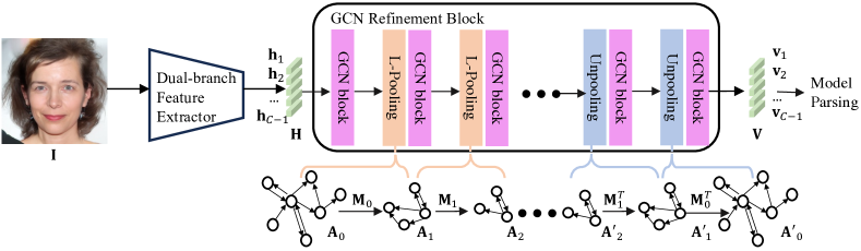
Figure 3: Learnable Graph Pooling Network. We first use the dual-branch feature extractor (Sec. 3.2.1) to extract the feature $\mathbf{H}$ given an input image $\mathbf{I}$. Then, the learned feature $\mathbf{H}$ is refined via the proposed GCN refinement block, which stacks different GCN layers with paired pooling-unpooling layers (Sec. 3.2.2). The GCN refinement block outputs the refined feature $\mathbf{V}$ that is used for model parsing. Our method is jointly trained with $3$ different objective functions (Sec. 3.3).

2 Related Works

The Reverse Engineering of Deception (RED) paradigm is a novel approach that aims to extract valuable information (e.g., adversarial perturbations, and used GMs) about machine-centric attacks [65, 21, 20, 49, 75, 67] that target machine learning decisions and human-centric attacks [70, 2, 27] that employ falsified media to deceive humans. In this work, our emphasis is on model parsing, a critical research problem within the RED framework, geared towards defending against human-centric attacks.

Unlike previous model parsing works [60, 50, 31, 4] that require prior knowledge of machine learning models and their inputs to predict training information or model hyperparameters, Asnani et al. [2] recently proposes a technique to estimate the $37$ pre-defined hyperparameters based on generated images. This work [2] uses a fingerprint estimation network is trained with four constraints to estimate the fingerprint for each image, which is then used to estimate hyperparameters. However, they overlook the dependencies among hyperparameters that cannot be adequately captured by the estimated mean and standard deviation.

Coordinate attacks detection [2] classify if two given images are generated from the same or different models. Coordinated attacks pose a challenge for existing image forensic approaches such as model attribution [70, 27] and CNN-generated image detection [64], which may struggle with performance when confronted with fake images generated by unseen GMs. In contrast, model parsing, which leverages predicted hyperparameters as descriptors for GMs, can effectively solve this challenging task. Unlike the previous work [2] that concludes one single partition experiment setup, we offer a more comprehensive analysis. Detecting CNN-generated image is extensively studied [73, 52, 27, 55, 33, 52, 51]. We also compare with the previous work in this detection task, showcasing the superiority of our method in detecting generation artifacts.

3 Method

In this section, we detail our proposed method. Sec. 3.1 first revisits fundamental concepts of model parsing and the process of formulating it into a graph node classification task. Sec. 3.2 introduces the proposed Learnabled Graph Pooling Network (LGPN). Lastly, we describe the training procedure and inference in Sec. 3.3 and Sec. 3.4, respectively.

3.1 Preliminaries

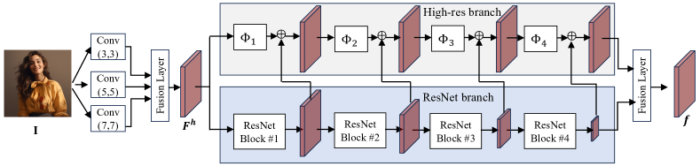
Figure 4: The dual-branch feature extractor. First, convolution layers with different kernel sizes extract feature maps of the input image $\mathbf{I}$. A fusion layer concatenates these feature maps and then proceeds the concatenated feature to the ResNet branch and High-res branch. ResNet branch consists of pre-trained ResNet blocks, while the high-res branch maintains the high-resolution representation to help detect generation artifacts. Lastly, output features of two branches are combined for down-stream tasks, such as model parsing and CNN-generated image detection.

3.1.1 Revisiting Reverse Engineering

Defined by work [2], hyperparameters that need to be parsed include discrete and continuous architecture parameters, as well as objective functions. The detailed definition is in Tab. 1 and 2 of the supplementary. For the discrete architecture parameters and objective functions, we compose a ground-truth vector ${\bf{y}}^{d}\in\mathbb{R}^{18}$ and ${\bf{y}}^{l}\in\mathbb{R}^{10}$, where each element is a binary value that indicates if the corresponding feature is used or not. For the continuous architecture parameters (e.g., layer number and parameter number), we use ${\bf{y}}^{c}\in\mathbb{R}^{9}$ as the ground truth vector, where each value is normalized into [$0$, $1$]. Predicting $\mathbf{y}^{d}$ and $\mathbf{y}^{l}$ is a classification task while the regression is used for $\mathbf{y}^{c}$.

The previous work collected $116$ different GMs (termed as RED$116$) to study the model parsing, but this dataset lacks comprehensive consideration about the recent proposed influential diffusion models. Therefore, we have augmented RED$116$ with different diffusion models such as DDPM [29], ADM [14] and Score-based DM [57], to increase the bandwidth spectrum of the GMs. More details are in the supplementary Sec. 4. Secondly, to make the trained model learn the generation artifacts, we have added real images to train these GMs into the dataset. In the end, we have collected $140$ GMs in total. We denote this dataset as RED$140$. Note that some public powerful text-to-image models, such as DALL-E$2$ and Midjourney, do not release their source code, such that it is challenging to curate detailed model hyperparameters of them. Therefore, we do not include them in the RED$140$.

3.1.2 Correlation Graph Construction

We first use conditional probability $P({L_{j}|L_{i}})$ to denote the probability of hyperparameter $L_{j}$ occurrence when hyperparameter $L_{i}$ appears. We count the occurrence of such a pair in the RED$140$ to retrieve the matrix $\mathbf{G}\in\mathbb{R}^{C\times C}$ ($C$ is the hyper-parameter number), and $\mathbf{G}_{ij}$ denotes the conditional probability of $P(L_{j}|L_{i})$. After that, we apply a fixed threshold $\tau$ to eliminate edges with low correlations. As a result, we obtain a directed graph $\mathbf{A}\in\mathbb{R}^{C\times C}$ and each element $\mathbf{A}_{ij}$ is a binary value that indicates if there exists an edge between node $i$ and $j$. In this graph data structure, we can leverage graph nodes and edges to represent hyperparameters and their dependencies, respectively.

Specifically, as depicted in Fig. 2b, each discrete hyperparameters (e.g., discrete architecture parameters and objective functions) is represented by one graph node, denoted as discrete-value graph node. For continuous hyperparameters (e.g., layer number and parameter number), we first divide the range into $n$ different intervals, and each of intervals is represented by one graph node, termed as continuous-value graph node. We formulate the model parsing as a graph node classification task, which helps learn the effective representation for each hyperparameters.

3.1.3 Stack Graph Convolution Layers

Let us revisit the basic formulation of Graph Convolution Network (GCN). Given the directed graph $\mathbf{A}$, we denote the stacked graph convolution operation as:

$$\mathbf{h}^{l}_{i}=\mathrm{ReLU}(\sum_{j=1}^{N}\mathbf{A}_{i,j}\mathbf{W}^{l}\mathbf{h}^{l-1}_{j}+\mathbf{b}^{l}),\vspace{-2mm}$$ (1)

where $\mathbf{h}^{l}_{i}$ represents the $i$-th node feature in graph $\mathbf{A}$, and $\mathbf{W}^{l}$ and $\mathbf{b}^{l}$ are corresponding weight and bias terms. We notice that different nodes in the graph have different degrees, which results in drastically different magnitudes for the aggregated node features. This can impair the node representation, because learning is always biased towards the high-degree nodes. To this end, we formulate the Eq. 1 into:

$$\mathbf{h}^{l}_{i}=\mathrm{ReLU}(\sum_{j=1}^{N}\mathbf{\hat{A}}_{i,j}\mathbf{W}^{l}\mathbf{h}^{l-1}_{j}/d_{i}+\mathbf{b}^{l}),\vspace{-2mm}$$ (2)

where $\mathbf{\hat{A}}=\mathbf{A}+\mathbf{I}$ and $\mathbf{I}$ is an $n\times n$ identity matrix, and $d_{i}$ is degree of node $i$, namely, $d_{i}=\sum^{n}_{j=1}\mathbf{\hat{A}}_{ij}$.

3.2 Learnable Graph Pooling Network

3.2.1 Dual-branch Feature Extractor

In the realm of image forensic, the specialized-design feature extractor is commonly used to learn distinguishing real and CNN-generated images [44, 64, 53, 17] or identifying the manipulation region [5, 16, 66, 77, 76]. Within the spectrum of established approaches, our work introduces a simple yet effective feature extractor, which is structured as a dual-branch network (Fig. 4) — given the input image, we use one branch (i.e., ResNet branch) to propagate the original image information, meanwhile, the other branch, denoted as high-res branch, harnesses the high-resolution representation that helps detect high-frequency generation artifacts stemming from various GMs.

More formally, given the image $\mathbf{I}\in\mathbb{R}^{3\times W\times H}$, we use three separate $2$D convolution layers with different kernel sizes (e.g., $3\times 3$, $5\times 5$ and $7\times 7$) to extract feature maps of $\mathbf{I}$. We concatenate these feature maps and feed them to the fusion layer — the $1\times 1$ convolution layer for the channel dimension reduction. As a result, we obtain the feature map $\mathbf{F}^{h}\in\mathbb{R}^{D\times W\times H}$, with the same height and width as $\mathbf{I}$. After that, we proceed $\mathbf{F}^{h}$ to the dual-branch backbone. Specifically, ResNet branch has four pre-trained ResNet blocks, commonly used as the generalized CNN-generated image detector [64, 51]. We upsample intermediate features output from each ResNet block and incorporate them into the high-res branch, as depicted in Fig. 4. The high-res branch also has four different convolution blocks (e.g., $\Phi_{b}$ with $b\in\{1\ldots 4\}$), which do not employ operations, such as the $2$D convolution with large strides and pooling layers, which spatially downsample learned feature maps. The utilization of the high-resolution representation is similar to the previous work [62, 6, 43, 27, 23] that also leverage such powerful representation for various image forensic tasks, whereas our dual-branch architecture is distinct to their approaches.

In the end, ResNet branch and high-res branch output feature maps are concatenated and then pass through an AVGPOOL layer. The final learned representation, $\mathbf{f}\in\mathbb{R}^{D}$, learns to capture generation artifacts of the given input image $\mathbf{I}$. We learn $C$ independent linear layers, i.e., $\Theta=\{{\theta_{i=0}^{C-1}}\}$ to transform $\mathbf{f}$ into a set of graph node features features $\mathbf{H}=\{\mathbf{h}_{0},\mathbf{h}_{1},...,\mathbf{h}_{(C-1)}\}$, which can form as a tensor, $\mathbf{H}\in\mathbb{R}^{C\times D}$. We use $\mathbf{H}$ to denote graph node features of the directed graph (i.e., graph topology) $\mathbf{A}\in\mathbb{R}^{C\times C}$.

3.2.2 GCN Refinement Block

The GCN refinement block has a learnable pooling-unpooling mechanism which progressively coarsens the original graph $\mathbf{A}_{0}$ into a series of coarsened graph $\mathbf{A}_{1},\mathbf{A}_{2}...\mathbf{A}_{n}$, and graph convolution is conducted on graphs at all different levels. Specifically, such a pooling operation is achieved by merging graph nodes, namely, via a learned matching matrix $\mathbf{M}$. Also, the correlation matrices of different graphs, denoted as $\mathbf{A}_{l}$ , are learned using MLP layers and are also influenced by the GM responsible for generating the input image. This further emphasizes the significant impact of the GM on the correlation graph generation process.

Learnable Graph Pooling Layer

First, $\mathbf{A}_{l}\in\mathbb{R}^{m\times m}$ and $\mathbf{A}_{l+1}\in\mathbb{R}^{n\times n}$ denote directed graphs at $l$ th and $l+1$ th layers, which have $m$ and $n$ ($m\geq n$) graph nodes, respectively. We use an assignment matrix $\mathbf{M}_{l}\in\mathbb{R}^{m\times n}$ to convert $\mathbf{A}_{l}$ to $\mathbf{A}_{l+1}$ as:

$$\mathbf{A}_{l+1}={\mathbf{M}_{l}}^{T}\mathbf{A}_{l}\mathbf{M}_{l}.$$ (3)

Also, we use $\mathbf{H}_{l}\in\mathbb{R}^{m\times D}$ and $\mathbf{H}_{l+1}\in\mathbb{R}^{n\times D}$ to denote graph node features of $\mathbf{A}_{l}$ and $\mathbf{A}_{l+1}$, where each graph node feature is $D$ dimensional. Therefore, we can use $\mathbf{M}_{l}$ to perform the graph node aggregation via:

$$\mathbf{H}_{l+1}={\mathbf{M}_{l}}^{T}\mathbf{H}_{l}.$$ (4)

For simplicity, we use $f_{GCN}$ to denote the mapping function that is imposed by a GCN block which has multiple GCN layers. $\mathbf{H}^{in}_{l}$ and $\mathbf{H}^{out}_{l}$ are the input and output feature of the $l$ th GCN blocks:

$$\mathbf{H}^{out}_{l}=f_{GCN}(\mathbf{H}^{in}_{l}).$$ (5)

Ideally, the pooling operation and correlation between different hyperparamters should be dependent the extracted feature of the given input image, $f$. Therefore, assuming the learned feature at $l$ th layer is $\mathbf{H}^{out}_{l}$, we use two separate weights $\mathbf{W_{m}}$ and $\mathbf{W_{a}}$ to learn the matching matrix $\mathbf{M}_{l}$ and adjacency matrix $\mathbf{A}_{l}$ at $l$ th layer as:

$$\mathbf{M}_{l+1}=\mathrm{softmax}(\mathbf{W_{m}}\mathbf{H}^{out}_{l}),$$ (6)

$$\mathbf{A}_{l+1}=\mathrm{sigmoid}(\mathbf{W_{a}}\mathbf{H}^{out}_{l}).$$ (7)

In fact, we modify the sigmoid function as $\frac{1}{1+e^{-\alpha x}}$, where $\alpha$ is set as $1e9$. As a result, we obtain the assignment matrix with values exclusively set to $0$ or $1$. After several levels of graph pooling, LGPN encodes information with an enlarged receptive field into the coarsened graph.

Learnable Unpooling Layer

We perform the graph unpooling operation, which restores and refines the information to the graph at the original resolution for the original graph node classification task. As depicted in Fig. 3, to avoid confusions, we use $\mathbf{H}$ and $\mathbf{V}$ to represent the graph node feature on the pooling and unpooling branch, respectively. The correlation matrix on the unpooling branch is denoted by $\mathbf{A}^{\prime}$.

$$\mathbf{A}^{\prime}_{l-1}=\mathbf{M}_{l}\mathbf{A}^{\prime}_{l}\mathbf{M}_{l}^{T},$$ (8)

$$\mathbf{V}_{l-1}={\mathbf{M}_{l}}\mathbf{V}_{l},$$ (9)

where $\mathbf{A}^{\prime}_{l}$ and $\mathbf{A}^{\prime}_{l-1}$ are the $l$ th and $l-1$ th layers in the unpooling branch. In the last, we use the refined feature $\mathbf{V}_{l}$ for the model parsing, as depicted in Fig. 3.

Discussion

This learnable pooling-unpooling mechanism offers three distinct advantages. Firstly, each supernode in the coarsened graph serves as the combination of features from its corresponding child nodes, and graph convolutions on supernodes have a large receptive field for aggregating the features. Secondly, the learnable correlation adapts and models hyperparameter dependencies dynamically based on generation artifacts of the input image feature (e.g., $\mathbf{H}$ or $\mathbf{V}$). Lastly, learned correlation graphs $\mathbf{A}$ vary across different levels, which effectively addresses the issue of over-smoothing commonly encountered in GCN learning [40, 46, 8]. Therefore, through this pooling-unpooling mechanism, we are able to learn a correlation between hyperparameters that is dependent on the GM used to generate the input image, thereby enhancing the performance of model parsing.

3.3 Training with Multiple Loss Functions

We jointly train our method by minimizing three losses: graph node classification loss $\mathcal{L}^{graph}$, generation artifacts isolation loss $\mathcal{L}^{iso}$ and hyperparameter hierarchy constraints $\mathcal{L}^{hier.}$, where $\mathcal{L}^{graph}$ encourages each graph node feature to predict the corresponding hyperparameter label, $\mathcal{L}^{iso}$ strives to project real and fake images into two separated manifolds, which helps the LGPN only parse the hyperparameters for generated images, and $\mathcal{L}^{hier}$ imposes hierarchical constraints among different hyperparameters while stabilizing the training.

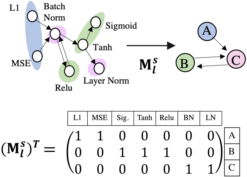
Figure 5: The toy example of the hyperparameter hierarchy assignment $\mathbf{M}^{s}$: both L1 and MSE belong to the category of pixel-level loss function, such that they are merged into the supernode A. Nonlinearity functions (e.g., ReLu and Tanh) and normalization methods (e.g., Layer Norm. and Batch Norm.) are merged into supernodes B and C, respectively.

Training Samples

Given a training sample denoted as $\{\mathbf{I},\mathbf{y}\}$, in which $\mathbf{I}$ is the input image and $\mathbf{y}=\{y_{0},y_{1},...,y_{(C-1)}\}$ is the corresponding annotation for parsed hyperparameters (e.g., loss functions, discrete and continuous architecture parameters) as introduced in Sec. 3.1.1. Specifically, $y_{c}$ is assigned as $1$ if the sample is annotated with category $c$ and $0$ otherwise, where $c\in\{0,1,...,C-1\}$. Empirically, $C$ is set as $55$: we use $28$ graph nodes to represent discrete hyperparameters (i.e., $10$ loss functions and $18$ discrete architecture parameters), and other $27$ nodes to represent $9$ continuous architecture parameters.

Graph Node Classification Loss

Given image $\mathbf{I}$, we convert the refined feature $\mathbf{V}$ into the predicted score vector, denoted as $\mathbf{s}=\{s_{0},s_{1},...,s_{(C-1)}\}$. We employ the sigmoid activation to retrieve the corresponding probability vector $\mathbf{p}=\{p_{0},p_{1},...,p_{(C-1)}\}$.

$$p_{c}=\sigma(s_{c}).$$ (10)

In general, cross entropy is used as the objective function, so we have:

$$\mathcal{L}^{graph}=\sum^{C-1}_{c=0}(y_{c}\log p_{c}+(1-y_{c})\log(1-p_{c})).$$ (11)

Hyperparameter Hierarchy Prediction

As depicted in Fig. 5, different hyperparameters can be grouped, so we define the hyperparameter hierarchy assignment $\mathbf{M}^{s}$ to reflect this inherent nature. More details of such the assignment are in supplementary Sec. 1. Suppose, at the layer $l$ th, we minimize the $L_{2}$ norm of the difference between the predicted matching matrix $\mathbf{M}_{l}$ and ${\mathbf{M}_{l}}^{s}$.

$$\mathcal{L}^{hier}={\lVert}{\mathbf{M}_{l}}^{s}-\mathbf{M}_{l}{\rVert}_{2}=\sqrt{\sum_{i=0}\sum_{j=0}({{m}^{s}}_{ij}-m_{ij}})^{2}$$ (12)

Generation Trace Isolation Loss

We denote the image-level binary label as $y^{img}$ and use $p^{img}$ to represents the probability that $\mathbf{I}$ is a generated image. Then we have:

$$\mathcal{L}^{iso}=\sum^{M-1}_{i=0}(y^{img}\log p^{img}+(1-y^{img})\log(1-p^{img})).$$ (13)

In summary, our joint training loss function can be written as $\mathcal{L}^{all}=\lambda_{1}\mathcal{L}^{graph}+\lambda_{2}\mathcal{L}^{hier}+\lambda_{3}\mathcal{L}^{iso}$, where $\lambda_{1}$ and $\lambda_{2}$ equal $0$ when $\mathbf{I}$ is real.

Method	Loss Function		Dis. Archi. Para.		Con. Archi. Para.
	F1 $\bf\uparrow$	Acc. $\bf\uparrow$	F1 $\bf\uparrow$	Acc. $\bf\uparrow$	L1 error $\bf\downarrow$
Random GT [2]	$0.636$	$0.716$	$0.529$	$0.575$	$0.184$
FEN [2]	$0.813$	$0.792$	$0.718$	$0.706$	$0.149$
FEN.∗ [2]	$0.801$	$0.811$	$0.701$	$0.708$	$0.146$
LGPN w/o GCN	$0.778$	$0.801$	$0.689$	$0.701$	$0.169$
LGPN w/o pooling	$0.790$	$0.831$	$0.698$	$0.720$	$0.145$
LGPN	$\mathbf{0.841}$	$\mathbf{0.833}$	$\mathbf{0.727}$	$\mathbf{0.755}$	$\mathbf{0.130}$

(a) The model parsing performance on RED$116$.

Method	Loss Function		Dis. Archi. Para.		Con. Archi. Para.
	F1 $\bf\uparrow$	Acc. $\bf\uparrow$	F1 $\bf\uparrow$	Acc. $\bf\uparrow$	L1 error $\bf\downarrow$
FEN. [2]	$0.793$	$0.807$	$0.691$	$0.707$	$0.156$
LGPN w/o GCN	$0.766$	$0.778$	$0.657$	$0.674$	$0.159$
LGPN w/o pooling	$0.819$	$0.823$	$0.710$	$0.732$	$0.122$
LGPN	$\mathbf{0.829}$	$\mathbf{0.840}$	$\mathbf{0.761}$	$\mathbf{0.753}$	$\mathbf{0.105}$

(b) The model parsing performance on RED$140$.

Table 1: We report the performance on parsing different hyperparameters, Loss Function reports the averaged prediction performance on $10$ objective functions. The averaged prediction performance on $18$ discrete architecture parameters and $9$ continuous architecture parameters are reported in Dis. Archi. Para. and Con. Archi. Para., respectively. [Bold: best result; $*$ means our reproduction with the public source code.]

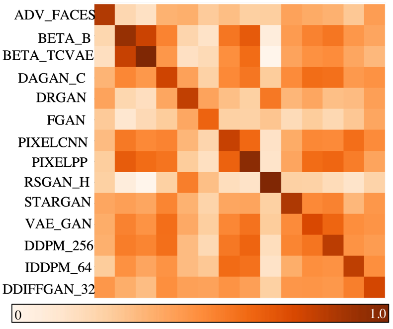
(a)

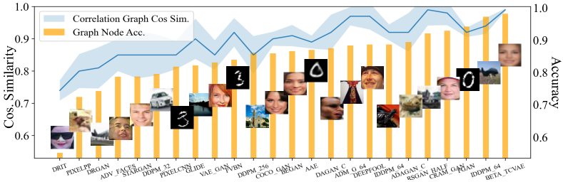
(b)

Figure 6: (a) Cosine similarity between generated correlation graphs for unseen GMs in one of four test sets. Each element of this matrix is the average cosine similarities of $2,000$ pairs of generated correlation graphs $\mathbf{A}$ from corresponding GMs. The diagonal of this matrix shows two images from the same GM have highly similar correlation graphs $\mathbf{A}$. The matrices for other three test sets are in Fig. 3 of the supplementary. (b) In the test set, GMs generate images with various contents (e.g., face, object and handwritten digits). We observe that for each GM, the cosine similarity between correlation graphs (i.e., $\mathbf{A}$) of two images ($3,000$ image pairs sampled) is positively correlated with the graph node classification accuracy achieved by LGPN on that particular GM. More results are in Fig. 4 of the supplementary.

3.4 Inference and Application

As depicted by Fig. 2c, we use the discrete-value graph node feature to perform the binary classification to decide the presence of given hyperparameters. For the continuous architecture, we first concatenate $n$ corresponding node feature and train a linear layer to regress it to the estimated value. Empirically, we set $n$ as $3$ and show this concatenated feature improves the robustness in predicting the continuous value, especially when we do not have an accurate prediction about continuous parameter range, detailed in the supplementary Sec. 3. Also, we apply the proposed method to two other applications: CNN-generated image detection and coordinate attacks identification. For CNN-generated image detection, we replace the GCN refinement module with a shallow network that takes learned features from the dual-branch feature extractor and outputs binary detection results, distinguishing generated images from real ones. Secondly, for coordinate attacks identification, we first denote the input image pair as ($\mathbf{I}_{1}$, $\mathbf{I}_{2}$), and we apply LGPN to obtain the refined feature ($\mathbf{V}_{1}$, $\mathbf{V}_{2}$). We use a shallow CNN to predict whether ($\mathbf{I}_{1}$, $\mathbf{I}_{2}$) are generated by the same GM.

4 Experiment

4.1 Model Parsing

Dataset and Metric

Each GM in the RED$116$ and RED$140$ contains $1,000$ images, and thus total numbers of generated images are $116,000$ and $140,000$, respectively. GMs in these two datasets are trained on real image datasets with various contents, including objects, handwritten digits, and human faces. Therefore, in RED$140$, we also include real images on which these GMs are trained. We follow the protocol of [2], where we have $4$ test sets, each comprising different GM categories, such as GAN, VAE, DM, etc. We train our model on the $104$ GMs from three test sets to predict $37$ hyperparameters. The evaluation is conducted on GMs in one remaining test set. The performance is averaged across four test sets, measured by F$1$ score and AUC for discrete hyperparameters (loss function and discrete architecture parameters) and L$1$ error for continuous architecture parameters. More details about datasets and implementations are in the supplementary Sec. 3.

Main Performance

We report the model parsing performance in Tab. 1. Our proposed method largely outperforms FEN and achieves state-of-the-art performance on both datasets. We also ablate our methods in various ways. First, we apply the dual-branch feature extractor with fully-connected layers to perform the model parsing, which achieves worse performance than FEN [2] in both RED$116$ and RED$140$ datasets, indicating naively adapting to model parsing does not produce the good performance. Second, we replace fully-connected layers with the GCN module without pooling, which is used to refine the learned feature for each hyperparameter. As a result, the performance increases, especially on parsing the loss functions (e.g., $3.0\%$ and $4.5\%$ higher accuracy in RED$116$ and RED$140$, respectively). This phenomenon is consistent with our statement that using a directed graph with GCN refinement modules can help capture the dependency among hyperparameters. However, simply stacking many layers of GCN results in the over-smoothing issue, imposing limitations on the performance. In our full LGPN model, such an issue can be reduced, and the overall performance achieves $5.1\%$ and $2.9\%$ higher F$1$ score than the model without pooling on parsing the loss function and discrete architecture parameters. Fig. 6(a) shows that correlation graphs generated from image pairs exhibit significant similarity when both images belong to the same unseen GM. This result demonstrates that our correlation graph largely depends on the GM instead of image content, given the fact that we have different contents (Fig. 6(b)) in unseen GMs from each test. Learning a GM-dependent correlation graph $\mathbf{A}$ is attributed to learning of generation artifacts by our dual-branch feature extractor, which has the high-resolution representation. Secondly, the learnable pooling-unpooling mechanism helps generate a series of generated graphs for different levels, which can be distinctive from each other. These variations in graph structure change graph neighbors for each node, enabling to reduction of the over-smoothing issue that always occurs on the deep GCN network. We provide more analysis about how the graph pooling alleviates the over-smoothing issue in the supplementary Sec. 3.

4.2 Image Synthesized Detection

Detection method	Variant	Generative Adversarial Networks						Deepfakes	Low level vision		Perceptual loss		Average
		Pro- GAN	Cycle- GAN	Big- GAN	Style- GAN	Gau- GAN	Star- GAN	FF++	SITD	SAN	CRN	IMLE
Trained network [64]	Blur+JPEG ($0.1$)	$\mathbf{{\color[rgb]{1,0,0}100.0}}$	$93.47$	$84.50$	$\mathbf{{\color[rgb]{0,0,1}99.54}}$	$89.49$	$98.15$	$89.02$	$73.75$	$59.47$	$98.24$	$98.40$	$89.45$
	Blur+JPEG ($0.5$)	$\mathbf{{\color[rgb]{1,0,0}100.0}}$	$96.83$	$88.24$	$98.29$	$98.09$	$95.44$	$66.27$	$86.0$	$61.2$	$\mathbf{{\color[rgb]{0,0,1}98.94}}$	$\mathbf{{\color[rgb]{0,0,1}99.52}}$	$89.89$
	ViT:CLIP ($0.5$)	$99.98$	$93.32$	$83.63$	$88.14$	$92.81$	$84.62$	$67.23$	$\mathbf{{\color[rgb]{0,0,1}93.48}}$	$55.21$	$88.75$	$96.22$	$85.77$
Patch classifier [7]	ResNet50-Layer1	$98.86$	$72.04$	$68.79$	$92.96$	$55.9$	$92.06$	$60.18$	$65.82$	$52.87$	$68.74$	$67.59$	$72.34$
	Xception-Block2	$80.88$	$72.84$	$71.66$	$85.75$	$65.99$	$69.25$	$76.55$	$76.19$	$76.34$	$74.52$	$68.52$	$74.41$
Co-occurence [47]	-	$99.74$	$80.95$	$50.61$	$98.63$	$53.11$	$67.99$	$59.14$	$68.98$	$60.42$	$73.06$	$87.21$	$72.72$
Freq-spec [72]	CycleGAN	$55.39$	$\mathbf{{\color[rgb]{1,0,0}100.0}}$	$75.08$	$55.11$	$66.08$	$\mathbf{{\color[rgb]{1,0,0}100.0}}$	$45.18$	$47.46$	$57.12$	$53.61$	$50.98$	$64.18$
Universal detector [51]	NN, $k=1$	$\mathbf{{\color[rgb]{1,0,0}100.0}}$	$98.14$	$94.49$	$86.68$	$\mathbf{{\color[rgb]{0,0,1}99.26}}$	$99.53$	$\mathbf{{\color[rgb]{0,0,1}93.09}}$	$78.46$	$67.54$	$83.13$	$91.07$	$90.12$
	LC	$\mathbf{{\color[rgb]{1,0,0}100.0}}$	$\mathbf{{\color[rgb]{0,0,1}99.46}}$	$\mathbf{{\color[rgb]{1,0,0}99.59}}$	$97.24$	$\mathbf{{\color[rgb]{1,0,0}99.98}}$	$99.60$	$82.45$	$61.32$	$\mathbf{{\color[rgb]{0,0,1}79.02}}$	$96.72$	$99.00$	$\mathbf{{\color[rgb]{0,0,1}92.21}}$
Ours		$\mathbf{{\color[rgb]{1,0,0}100.0}}$	$97.03$	$\mathbf{{\color[rgb]{0,0,1}97.76}}$	$\mathbf{{\color[rgb]{1,0,0}99.96}}$	$98.97$	$\mathbf{{\color[rgb]{0,0,1}99.65}}$	$\mathbf{{\color[rgb]{1,0,0}93.50}}$	$\mathbf{{\color[rgb]{1,0,0}98.42}}$	$\mathbf{{\color[rgb]{1,0,0}85.00}}$	$\mathbf{{\color[rgb]{1,0,0}99.60}}$	$\mathbf{{\color[rgb]{1,0,0}99.90}}$	$\mathbf{{\color[rgb]{1,0,0}97.27}}$

Table 2: CNN-synthesized image detection performance measured by Average Precision on $13$ forgery methods containing face and non-face images. Previous methods’ quantitative results are taken from [51]. [Bold: best result; Bold: second best result].

Detection method	Deep fakes	Diffusion models						Average
	Celeb- DF	DD- PM	DD- IM	GLIDE	LDM	DALL- E2	Mid Journey
ResNet ($0.1$) [64]	$89.0$	$72.33$	$70.11$	$69.4$	$80.55$	$72.4$	$57.5$	$73.04$
ResNet ($0.5$) [64]	$84.5$	$71.04$	$67.54$	$71.3$	$75.20$	$74.1$	$64.3$	$72.53$
Ours	$\mathbf{91.11}$	$\mathbf{90.59}$	$\mathbf{88.00}$	$\mathbf{93.19}$	$\mathbf{93.91}$	$\mathbf{95.1}$	$\mathbf{70.0}$	$\mathbf{89.28}$

Table 3: CNN-synthesized image detection performance by Average Precision on additional images generated via deepfakes (e.g., Celeb-DF [42]) and diffusion models. [Bold: best result].

For CNN-generated image detection, we follow the prior works [64, 51, 72], which train the model on images generated by ProGAN [34], and tests on images generated by other unseen GMs. As shown in Tab. 2 and 3, our proposed method achieves the best overall detection performance. We believe this is because the dual-branch feature extractor uses the high-resolution branch to exploit more high-frequency generation artifacts. In Tab. 2, we do not follow the diffusion models detection performance reported by [51], since they only release $\frac{1}{10}$ used test set. Instead, Tab. 3 reports our detection performance on diffusion models, which $10$k images collected for each category, and Celeb-DF [41].

4.3 Coordinate Attack Detection

We evaluate coordinated attacks detection on RED$140$ in a $4$-fold cross validation. In each fold, the train set has $125$ GMs, and the test set has $30$ GMs where $15$ GMs are exclusive from the train set and $15$ GMs are seen in the train set. We use the average of the $4$ folds as the final result. For the measurement, we use accuracy, AUC and probability of detection at a fixed false alarm rate (Pd@FAR) e.g., Pd@$5\%$ and Pd@$1\%$. These metrics are commonly used in bio-metric applications [24, 25, 1]. Specifically, aside from FEN [2], we also compare with the very recent work HiFi-Net [27], since HiFi-Net demonstrates SoTA results in attributing different forgery methods, which can be used to decide if two images generated from the same GM. Specifically, we train HiFi-Net to classify $125$ GMs and take learned features from the last fully-connected layer for the coordinated attack detection. The performance is reported in Tab. 4(a). We observe the HiFi-Net performance is much worse than the model parsing baseline model (e.g., LGPN w/o pooling.) and FEN, which is around $20\%$ AUC lower. Tab. 7(a) shows the FEN and LGPN have comparable performance with HiFi-Net on seen GMs (first two bar charts), yet performance gains over HiFi-Net are substantially enlarged when images are generated by unseen GMs (last three bar charts). Lastly, LGPN has a better Pd@$5\%$ performance than other methods.

Method	Acc.	AUC	Pd@$5$%
HiFi. [27]	$72.3$	$75.4$	$30.4$
FEN. [2]	$83.0$	$92.4$	$61.2$
LGPN w/o GCN	$83.9$	$92.2$	$62.5$
LGPN w/o pooling	$86.6$	$94.2$	$68.6$
LGPN∗	$87.9$	$95.7$	$72.3$

(a)

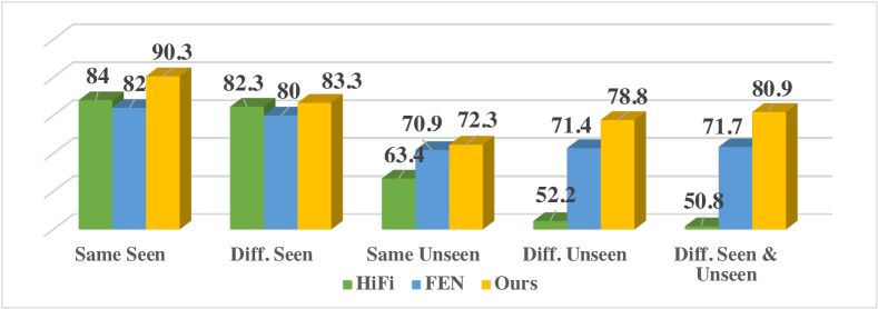
(a)

Table 4: The coordinate attack detection performance. (a) The average performance on $4$ folds cross validation. (b) Same Seen and Diff. Seen mean same and different GMs in seen GMs. Same Unseen and Diff Unseen mean same and different GMs in unseen GMs. Diff. means images from one seen and one unseen GMs.

5 Conclusion

In this study, we propose a novel method that incorporates a learnable pooling-unpooling mechanism for the model parsing. In addition, we provide a dual-branch feature extractor to help detect generation artifacts, which proves effective in CNN-generated image detection and coordinated attack identification.

Limitation

While our proposed data-driven model parsing approach delivers excellent performance on the collected RED$140$ dataset, it is worth exploring their effectiveness on specific GMs that fall outside our dataset scope.

Supplementary Material

In this supplementary, we provide:

$\diamond$ Predictable hyperparameters introduction.

$\diamond$ Training and implementation details.

$\diamond$ Additional results of model parsing and CNN-generated image detection.

$\diamond$ The construction of RED$140$ dataset.

$\diamond$ Hyperparameter ground truth and the model parsing performance for each GM

Table 1: Loss Function types used by all GMs. We group the $10$ loss functions into three categories. We use the binary representation to indicate the presence of each loss type in training the respective GM.

Category	Loss Function
Pixel-level	$L_{1}$
	$L_{2}$
	Mean squared error (MSE)
	Maximum mean discrepancy (MMD)
	Least squares (LS)
Discriminator	Wasserstein loss for GAN (WGAN)
	Kullback–Leibler (KL) divergence
	Adversarial
	Hinge
Classification	Cross-entropy (CE)

Table 2: Discrete Architecture Parameters used by all GMs. We group the $18$ discrete architecture hyperparameters into $6$ categories. We use the binary representation to indicate the presence of each parameter type in training the respective GM.

Category	Discrete Architecture Parameters
Normalization	Batch Normalization
	Instance Normalization
	Adaptive Instance Normalization
	Group Normalization
Nonlinearity in the Last Layer	ReLU
	Tanh
	Leaky_ReLU
	Sigmoid
	SiLU
Nonlinearity in the Last Block	ELU
	ReLU
	Leaky_ReLU
	Sigmoid
	SiLU
Up-sampling	Nearest Neighbour Up-sampling
	Deconvolution
Skip Connection	Feature used
Down-sampling	Feature used

Table 3: Continuous Architecture Parameters used by all GMs, where ”[” denotes inclusive and ”(” denotes exclusive intervals. We report the range for $9$ continuous parameters.

Category	Range	Discrete Architecture Parameters
Layer Number	$(0\text{---}717]$	Layers Number
	$[0\text{---}289]$	Convolution Layer Number
	$[0\text{---}185]$	Fully-connected Layer Number
	$[0\text{---}46]$	Pooling Layer Number
	$[0\text{---}235]$	Normalization Layer Number
	$(0\text{---}20]$	Layer Number per Block
Unit Number	$(0\text{---}8,365]$	Filter Number
	$(0\text{---}155]$	Block Number
	$(0\text{---}56,008,488]$	Parameter Number

1 Predictable Hyperparameters Introduction

In this study, we investigate $37$ hyperparameters that exhibit the predictability according to Asnani et al. [2]. These hyperparameters are categorized into three groups: (1) Loss Function (Tab. 1), (2) Discrete Architecture Parameters (Tab. 2), (3) Continuous Architecture Parameters (Tab. 3). We report our proposed method performance of parsing hyperparameters in these three groups via Fig. 1(a), Fig. 1(b), and Fig. 1(c), respectively. Moreover, in the main paper’s Eq. 12 and Fig. 5, we employ the assignment hierarchy $\mathbf{M}^{s}$ to group different hyperparameters together, which supervises the learning of the matching matrix $\mathbf{M}$. The construction of such the $\mathbf{M}^{s}$ is also based on Tab. 1, 2, and 3, which not only define three coarse-level categories, but also fine-grained categories such as pixel-level objective (loss) function (e.g., L1 and MSE) in Tab. 1, and normalization methods (e.g., ReLu and Tanh) as well as nonlinearity functions (e.g., Layer Norm. and Batch Norm.) in Tab. 2.

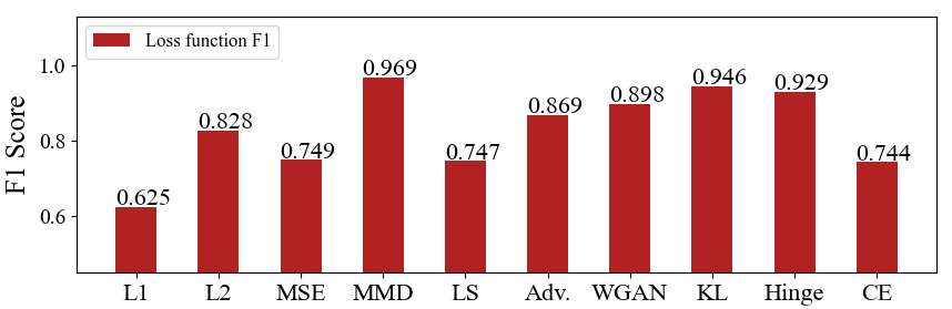
(a)

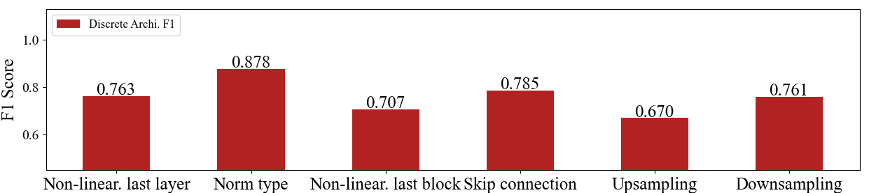
(b)

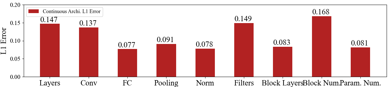
(c)

Figure 1: (a) The F$1$score on the loss function reveals that MMD and KL are two easiest loss functions to predict. (b) The F$1$score on the discrete architecture parameters demonstrates that predicting these parameters is more challenging than predicting the loss function. This finding aligns with the empirical results reported in the previous work [2]. (c) The L$1$ error on the continuous architecture parameters indicates that it is challenging to predict Block Num. and Filter Num..

Table 4: Using different $n$ graph nodes for the continuous hyperparameter regression.

$n$ Value	$2$	$3$	$4$	$5$	$6$
L1 Error	$0.108$	$0.105$	$0.106$	$0.112$	$0.120$

2 Training and Implementation Details

Training Details

Given the directed graph $\mathbf{A}\in\mathbb{R}^{C\times C}$, which contains $C$ graph nodes. We empirically set $C$ as $55$, as mentioned in the main paper Sec. 3.3. In the training, LGPN takes the given image $\mathbf{I}$ and output the refined feature $\mathbf{V}\in\mathbb{R}^{55\times D}$, which contains learned features for each graph node, namely, $\mathbf{V}=\{\mathbf{v}_{0},\mathbf{v}_{1},...,\mathbf{v}_{54}\}$. As a matter of fact, we can view $\mathbf{V}$ as three separate sections: $\mathbf{V}^{l}=\{\mathbf{v}_{0},\mathbf{v}_{1},...,\mathbf{v}_{9}\}$, $\mathbf{V}^{d}=\{\mathbf{v}_{10},\mathbf{v}_{11},...,\mathbf{v}_{27}\}$, and $\mathbf{V}^{c}=\{\mathbf{v}_{28},\mathbf{v}_{29},...,\mathbf{v}_{54}\}$, which denote learned features for graph nodes of $10$ loss function (e.g., L1 and MSE), $18$ discrete architecture parameter (e.g., Batch Norm. and ReLU), and $9$ continuous architecture parameter (i.e., Parameter Num.), respectively. Note $\mathbf{V}^{c}$ represents learned features of $9$ continuous architecture parameters, because each continuous hyperparameter is represented by $3$ graph nodes, as illustrated in Fig. 2c of the main paper.

Furthermore, via Eq. 10 in the main paper, we use $\mathbf{V}$ to obtain the corresponding probability score $\mathbf{p}=\{p_{0},p_{1},...,p_{54}\}$ for each graph node. Similar to $\mathbf{V}$, this $\mathbf{p}$ can be viewed as three sections: $\mathbf{p}^{l}\in\mathbb{R}^{10}$, $\mathbf{p}^{d}\in\mathbb{R}^{18}$ and $\mathbf{p}^{c}\in\mathbb{R}^{27}$ for loss functions, discrete architecture hyperparameters, continuous architecture hyperparameters, respectively. In the end, we use $\mathbf{p}$ to help optimize LGPN via the graph node classification loss (Eq. 11). After the training converges, we further apply $9$ individual fully-connected layers on the top of frozen learned features of continuous architecture parameters (e.g., $\mathbf{V}^{c}$). via minimizing the $\mathcal{L}_{1}$ distance between predicted and ground truth value.

In the inference (the main paper Fig. 2c), for loss function and discrete architecture parameters, we use output probabilities (e.g., $\mathbf{p}^{l}$ and $\mathbf{p}^{d}$) of discrete value graph nodes, for the binary “used v.s. not” classification. For the continuous architecture parameters, we first concatenate learned features of corresponding graph nodes. We utilize such a concatenated feature with pre-trained fully-connected layers to estimate the continuous hyperparameter value.

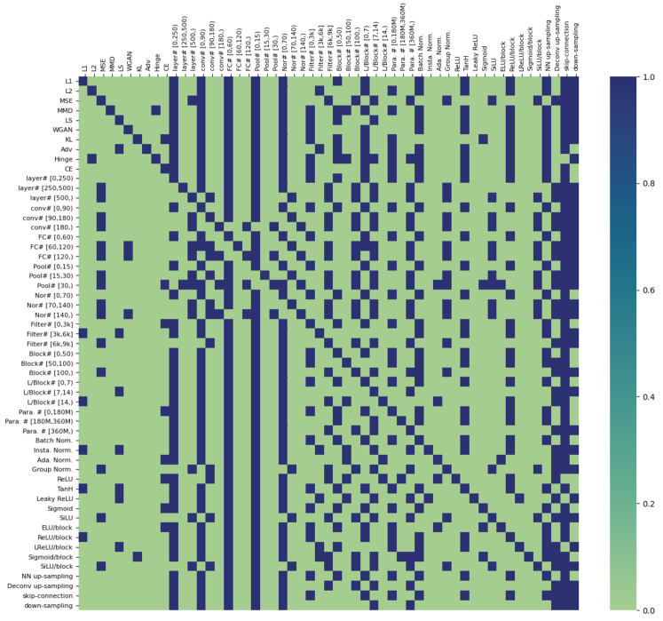
Figure 2: The initial correlation graph $\mathbf{A}$ that we construct based on the probability table in Sec. 3.1.2 of the main paper. The optimum threshold we use is $0.45$.

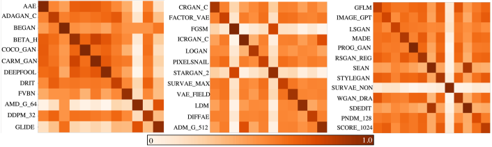
Figure 3: Each element of these two matrices is the average cosine similarities of $2,000$ pairs of generated correlation graphs $\mathbf{A}$ from corresponding GMs in the second, third and forth test sets.

Implementation Details

Denote the output feature from the dual-branch feature extractor as $\mathbf{f}\in\mathbb{R}^{2048}$. To transform $f$ into a set of features $\mathbf{H}=\{\mathbf{h}_{0},\mathbf{h}_{1},...,\mathbf{h}_{54}\}$ for the $55$ graph nodes, $55$ independent linear layers ($\Theta$) are employed. Each feature $h_{i}$ is of dimension $\mathbb{R}^{128}$. The $\mathbf{H}$ is fed to the GCN refinement block, which contains $5$ GCN blocks, each of which has $2$ stacked GCN layers. In other words, the GCN refinement block has $10$ layers in total. We use the correlation graph $\mathbf{A}\in\mathbb{R}^{55\times 55}$ (Fig. 2) to capture the hyperparameter dependency and during the training the LGPN pools $\mathbf{A}$ into $\mathbf{A}_{1}\in\mathbb{R}^{18\times 18}$ and $\mathbf{A}_{2}\in\mathbb{R}^{6\times 6}$ as the Fig. 3 of the main paper. The LGPN is implemented using the PyTorch framework. During training, a learning rate of 3e-2 is used. The training is performed with a batch size of $400$, where $200$ images are generated by various GMs and $200$ images are real. To enhance learning the high-resolution representation to capture generation artifacts, we increase the learning rate on the high-res branch as 5e-2. We use ReduceLROnPlateau as the scheduler to adjust the learning rate based on the validation loss.

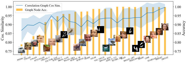
Figure 4: For each GM in the third and forth test sets, the positive correlation between the cosine similarity between image pairs’s correlation graphs (i.e., $\mathbf{A}$) and the graph node classification accuracy achieved by LGPN on that particular GM. This positive correlation demonstrates that the correlation graph is important to the performance of the graph node classification, which encourages the LGPN to learn the representation for each hyperparameter.

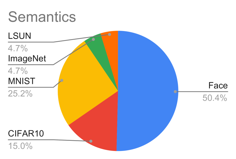
(a)

(b)

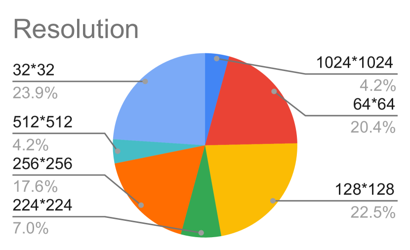
(c)

Figure 5: RED$140$ statistics. (a) The dataset is trained on various image contents or semantics. (b) The real-image category contains many real-image datasets that GMs are trained on [35, 34, 13, 69, 26, 38, 39]. (c) The GM has various image resolutions.

3 Additional Results

In Fig. 6 of the main paper, we visualize the correlation graph similarities among different GMs and the relationship between graph node classification and GM correlation graph similarity for GMs in the first and second test set. In this section, we offer a similar visualization (e.g., Fig. 3 and Fig. 4) for other test sets. In main paper’s Sec 3.4, we use $n$ graph nodes for each continuous hyperparameter and $n$ is set as $3$. Tab. 4 shows the advantage of choice, which shows the lowest $\mathcal{L}_{1}$ regression error is achieved when $n$ is $3$.

Furthermore, in addition to Tab. 2 and 3 of the main paper, we provide the CNN-generated image detection performance measured by Accuracy in Tab. 6 and 7.

(a)

(b)

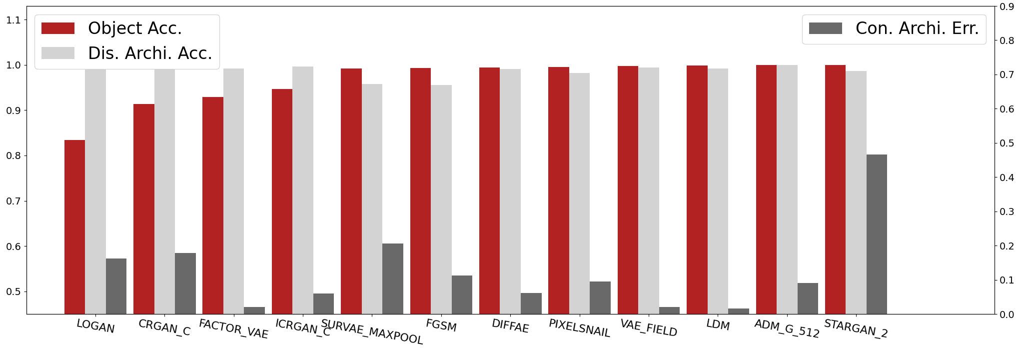
(c)

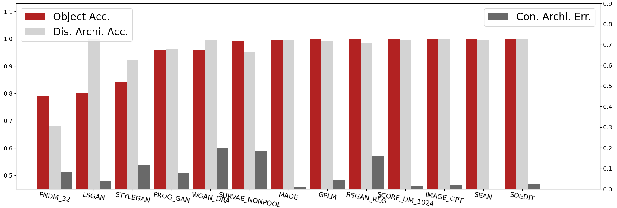
(d)

Figure 6: We report detailed model parsing results on different GMs in each test set. These results include loss function and discrete architecture parameters prediction accuracy, as well as the L$1$ error on the continuous architecture parameter prediction. Specifically, (a), (b), (c), and (d) are the performance for GMs in the $1$st, $2$nd, $3$rd and $4$th test set, respectively.

4 RED$140$ Dataset

In this section, we provide an overview of the RED$140$ dataset, which is used for both model parsing and coordinated attack detection. Note that, for the experiment reported in Tab. 1a of the main paper, we follow the test sets defined in RED$116$ [2]. When we construct RED$140$, we use images from ImageNet, FFHQ, CelebHQ, CIFAR10 and LSUN as the real-images category of RED$140$, nd exclude GM that is not trained on the real-image category of RED$140$. In addition, both RED$116$ and RED$140$ contain various image content and resolution, and the details about RED$140$ is uncovered in Fig. 5. For test sets (Tab. 5), we follow the dataset partition of RED$116$, whereas excluding the GMs that is trained on real images which RED$140$ does have. For example, JFT-$300$M is used to train BigGAN, so we remove BIGGAN_128, BIGGAN_256 and BIGGAN_512 in the first, second and third test sets.

Table 5: Test sets used for evaluation. Each set contains generative models from GAN, DM, VAE, AR (Auto-Regressive), AA (Adversarial Attack) and NF (Normalizing Flow). All test sets contain face and non-face in the image content. [Keys: R means GM is used in the test set of RED$116$ but is not used in RED$140$.]

Set $1$	Set $2$	Set $3$	Set $4$
ADV_FACES	AAE	BICYCLE_GAN (R)	GFLM
BETA_B	ADAGAN_C	BIGGAN_512 (R)	IMAGE_GPT
BETA_TCVAE	BEGAN	CRGAN_C	LSGAN
BIGGAN_128 (R)	BETA_H	FACTOR_VAE	MADE
DAGAN_C	BIGGAN_256 (R)	FGSM	PIX2PIX (R)
DRGAN	COCOGAN	ICRGAN_C	PROG_GAN
FGAN	CRAMERGAN	LOGAN	RSGAN_REG
PIXEL_CNN	DEEPFOOL	MUNIT (R)	SEAN
PIXEL_CNN++	DRIT	PIXEL_SNAIL	STYLE_GAN
RSGAN_HALF	FAST_PIXEL(R)	STARGAN_2	SURVAE_FLOW_NONPOOL
STARGAN	FVBN	SURVAE_FLOW_MAXPOOL	WGAN_DRA
VAEGAN	SRFLOW (R)	VAE_FIELD	YLG (R)
DDPM_256	ADM-G_64	LDM	PNDM_32
IDDPM_64	DDPM_32	Diffae_256	SCORE_DM_1024
Denoise_GAN_32	GLIDE	ADM-G_512	SEDdit

5 GM Hyperparameter Ground Truth

In this section, we report the ground truth vector of different hyperparameters of each GM contained in the RED$140$. Specifically, Tab. 8 and Tab. 9 report the loss function ground truth vector for each GM. Tab. 10 and Tab. 11 report the discrete architecture parameter ground truth for each GM. Tab. 12 and Tab. 13 report the discrete architecture parameter ground truth for each GM. The detailed model parsing performance on each GM is reported in Fig. 6.

Figure 7: Collected images from DALL-E2 and Midjourney. From top to down, different rows represent different image categories: person, bedroom, and church. In each row, the first and last $4$ images are from DALL-E2 and Midjourney, respectively.

Detection method	Variant	Generative Adversarial Networks						Deepfakes	Low level vision		Perceptual loss		Average
		Pro- GAN	Cycle- GAN	Big- GAN	Style- GAN	Gau- GAN	Star- GAN	FF++	SITD	SAN	CRN	IMLE
Trained network [64]	Blur+JPEG ($0.1$)	$99.90$	$85.20$	$70.20$	$85.70$	$78.95$	$91.70$	$53.47$	$66.67$	$48.69$	$86.31$	$86.26$	$77.46$
	Blur+JPEG ($0.5$)	$\mathbf{{\color[rgb]{1,0,0}100.0}}$	$80.77$	$58.98$	$69.24$	$79.25$	$80.94$	$51.06$	$56.94$	$47.73$	$87.58$	$\mathbf{{\color[rgb]{0,0,1}94.07}}$	$73.32$
	ViT:CLIP ($0.5$)	$98.94$	$78.80$	$60.62$	$60.56$	$66.82$	$62.31$	$52.28$	$65.28$	$47.97$	$64.09$	$80.00$	$67.02$
Patch classifier [7]	ResNet50-Layer1	$94.38$	$67.38$	$64.62$	$82.26$	$57.19$	$80.29$	$55.32$	$64.59$	$51.24$	$54.29$	$55.11$	$66.06$
	Xception-Block2	$75.03$	$68.97$	$68.47$	$79.16$	$64.23$	$63.94$	$75.54$	$\mathbf{{\color[rgb]{0,0,1}75.00}}$	$\mathbf{{\color[rgb]{1,0,0}75.00}}$	$\mathbf{{\color[rgb]{0,0,1}72.00}}$	$55.52$	$70.31$
Co-occurence [47]	-	$97.70$	$63.15$	$53.75$	$\mathbf{{\color[rgb]{0,0,1}92.50}}$	$51.10$	$54.70$	$57.10$	$63.00$	$\mathbf{{\color[rgb]{0,0,1}58.02}}$	$65.65$	$66.00$	$65.49$
Freq-spec [72]	CycleGAN	$49.90$	$\mathbf{{\color[rgb]{1,0,0}99.99}}$	$50.50$	$49.90$	$50.30$	$\mathbf{{\color[rgb]{0,0,1}99.70}}$	$50.10$	$50.00$	$48.00$	$51.00$	$50.00$	$59.00$
Universal detector [51]	NN, $k=1$	$99.58$	$94.70$	$86.95$	$80.24$	$\mathbf{{\color[rgb]{0,0,1}96.67}}$	$98.84$	$\mathbf{{\color[rgb]{1,0,0}80.90}}$	$71.00$	$56.00$	$66.00$	$77.10$	$\mathbf{{\color[rgb]{0,0,1}82.52}}$
	LC	$\mathbf{{\color[rgb]{1,0,0}100.0}}$	$\mathbf{{\color[rgb]{0,0,1}98.50}}$	$\mathbf{{\color[rgb]{0,0,1}94.50}}$	$82.00$	$\mathbf{{\color[rgb]{1,0,0}99.50}}$	$97.00$	$\mathbf{{\color[rgb]{0,0,1}66.60}}$	$63.00$	$58.00$	$60.00$	$72.00$	$81.00$
Ours		$\mathbf{{\color[rgb]{1,0,0}100.0}}$	$93.75$	$\mathbf{{\color[rgb]{1,0,0}94.60}}$	$\mathbf{{\color[rgb]{1,0,0}97.02}}$	$94.93$	$\mathbf{{\color[rgb]{1,0,0}99.92}}$	$52.76$	$\mathbf{{\color[rgb]{1,0,0}90.27}}$	$52.96$	$\mathbf{{\color[rgb]{1,0,0}98.16}}$	$\mathbf{{\color[rgb]{1,0,0}98.28}}$	$\mathbf{{\color[rgb]{1,0,0}88.02}}$

Table 6: CNN-generated image detection performance measured by Accuracy, on $13$ forgery methods containing face and non-face images. Previous methods’ quantitative results are taken from [51]. [Bold: best result; Bold: second best result].

Detection method	Deep fakes	Diffusion models						Average
	Celeb- DF	DD- PM	DD- IM	GLIDE	LDM	DALL- E2	Mid Journey
ResNet ($0.1$) [64]	$64.2$	$63.1$	$64.7$	$71.2$	$63.6$	$50.5$	$56.8$	$62.01$
ResNet ($0.5$) [64]	$60.9$	$68.9$	$56.3$	$68.4$	$52.7$	$51.3$	$54.2$	$58.95$
Ours	$\mathbf{89.2}$	$\mathbf{90.4}$	$\mathbf{90.3}$	$\mathbf{94.2}$	$\mathbf{84.7}$	$\mathbf{53.4}$	$\mathbf{55.8}$	$\mathbf{79.71}$

Table 7: CNN-generated image detection performance by Accuracy, on additional images generated via deepfakes (e.g., Celeb-DF) and diffusion models. [Bold: best result].

Table 8: Ground truth Loss Function feature vector used for prediction of loss type for all GMs. The loss function ground truth is in (Tab. 1).

GM	$L_{1}$	$L_{2}$	MSE	MMD	LS	WGAN	KL	Adversarial	Hinge	CE
AAE	$1$	$0$	$0$	$0$	$0$	$0$	$0$	$0$	$0$	$1$
ACGAN	$1$	$0$	$0$	$0$	$0$	$0$	$0$	$0$	$0$	$1$
ADAGAN_C	$0$	$0$	$0$	$0$	$1$	$0$	$0$	$0$	$0$	$1$
ADAGAN_P	$0$	$0$	$0$	$0$	$1$	$0$	$0$	$0$	$0$	$0$
ADM_G_64	$0$	$0$	$1$	$0$	$0$	$0$	$0$	$0$	$0$	$0$
ADM_G_128	$0$	$0$	$1$	$0$	$0$	$0$	$0$	$0$	$0$	$0$
ADM_G_256	$0$	$0$	$1$	$0$	$0$	$0$	$0$	$0$	$0$	$0$
ADM_G_512	$0$	$0$	$1$	$0$	$0$	$0$	$0$	$0$	$0$	$0$
ADV_FACES	$1$	$0$	$1$	$0$	$1$	$0$	$0$	$0$	$0$	$0$
ALAE	$0$	$0$	$1$	$0$	$1$	$0$	$0$	$0$	$0$	$0$
BEGAN	$1$	$0$	$0$	$0$	$0$	$0$	$0$	$0$	$0$	$0$
BETA_B	$0$	$0$	$0$	$0$	$0$	$0$	$1$	$0$	$0$	$1$
BETA_H	$0$	$0$	$0$	$0$	$0$	$0$	$1$	$0$	$0$	$1$
BETA_TCVAE	$1$	$0$	$0$	$0$	$0$	$0$	$1$	$0$	$0$	$1$
BGAN	$0$	$0$	$0$	$0$	$1$	$0$	$0$	$0$	$0$	$1$
BICYCLE_GAN	$1$	$0$	$1$	$0$	$0$	$0$	$1$	$0$	$0$	$0$
BIGGAN_128	$1$	$0$	$0$	$0$	$0$	$0$	$0$	$0$	$0$	$0$
BIGGAN_256	$1$	$0$	$0$	$0$	$0$	$0$	$0$	$0$	$0$	$0$
BIGGAN_512	$1$	$0$	$0$	$0$	$0$	$0$	$0$	$0$	$0$	$0$
Blended_DM	$0$	$0$	$1$	$0$	$0$	$0$	$0$	$0$	$0$	$0$
CADGAN	$0$	$0$	$0$	$1$	$0$	$0$	$0$	$0$	$0$	$0$
CCGAN	$0$	$0$	$0$	$0$	$1$	$0$	$0$	$1$	$0$	$0$
CGAN	$0$	$0$	$1$	$0$	$1$	$0$	$0$	$0$	$0$	$0$
CLIPDM	$0$	$0$	$1$	$0$	$0$	$0$	$0$	$0$	$0$	$0$
COCO_GAN	$1$	$1$	$0$	$0$	$0$	$1$	$0$	$0$	$1$	$0$
COGAN	$0$	$0$	$0$	$0$	$1$	$0$	$0$	$0$	$0$	$0$
COLOUR_GAN	$1$	$0$	$0$	$0$	$1$	$0$	$0$	$0$	$0$	$0$
CONT_ENC	$0$	$1$	$0$	$0$	$1$	$0$	$0$	$0$	$0$	$0$
CONTRAGAN	$1$	$0$	$0$	$0$	$0$	$0$	$0$	$1$	$0$	$1$
COUNCIL_GAN	$1$	$0$	$1$	$0$	$1$	$0$	$0$	$0$	$0$	$0$
CRAMER_GAN	$0$	$0$	$0$	$0$	$0$	$1$	$0$	$0$	$0$	$0$
CRGAN_C	$1$	$1$	$0$	$0$	$0$	$0$	$0$	$0$	$0$	$1$
CRGAN_P	$1$	$1$	$0$	$0$	$0$	$0$	$0$	$0$	$0$	$0$
CYCLEGAN	$1$	$0$	$0$	$0$	$1$	$0$	$0$	$0$	$0$	$0$
DAGAN_C	$1$	$0$	$0$	$0$	$0$	$0$	$0$	$0$	$0$	$1$
DAGAN_P	$1$	$0$	$0$	$0$	$0$	$0$	$0$	$0$	$0$	$0$
DCGAN	$0$	$0$	$0$	$0$	$0$	$0$	$0$	$0$	$0$	$1$
DDPM_32	$0$	$0$	$1$	$0$	$0$	$0$	$0$	$0$	$0$	$0$
DDPM_256	$0$	$0$	$1$	$0$	$0$	$0$	$0$	$0$	$0$	$0$
DDiFFGAN_32	$0$	$0$	$1$	$0$	$0$	$1$	$0$	$0$	$0$	$0$
DDiFFGAN_256	$0$	$0$	$1$	$0$	$0$	$1$	$0$	$0$	$0$	$0$
DEEPFOOL	$1$	$1$	$0$	$0$	$0$	$0$	$0$	$0$	$0$	$0$
DFCVAE	$0$	$1$	$0$	$0$	$0$	$0$	$1$	$0$	$0$	$1$
DIFFAE_$256$	$0$	$0$	$1$	$0$	$0$	$0$	$0$	$0$	$0$	$0$
DIFFAE_LATENT	$0$	$0$	$1$	$0$	$0$	$0$	$0$	$0$	$0$	$0$
DIFF-ProGAN	$0$	$0$	$0$	$0$	$0$	$0$	$1$	$0$	$0$	$0$
DIFF-StyleGAN	$0$	$0$	$0$	$0$	$0$	$0$	$1$	$0$	$0$	$0$
DIFF-ISGEN	$0$	$0$	$0$	$0$	$0$	$0$	$1$	$0$	$0$	$0$
DISCOGAN	$1$	$0$	$0$	$0$	$1$	$0$	$0$	$0$	$0$	$0$
DRGAN	$0$	$0$	$0$	$0$	$1$	$0$	$0$	$0$	$0$	$1$
DRIT	$1$	$0$	$0$	$0$	$1$	$0$	$0$	$0$	$0$	$1$
DUALGAN	$1$	$0$	$0$	$0$	$0$	$1$	$0$	$0$	$0$	$0$
EBGAN	$0$	$1$	$0$	$0$	$1$	$0$	$0$	$1$	$1$	$0$
ESRGAN	$1$	$0$	$0$	$0$	$1$	$0$	$0$	$0$	$0$	$0$
FACTOR_VAE	$1$	$0$	$0$	$0$	$0$	$0$	$1$	$0$	$0$	$1$
Fast pixel	$0$	$0$	$0$	$0$	$0$	$0$	$0$	$0$	$0$	$1$
FFGAN	$1$	$1$	$0$	$0$	$1$	$0$	$0$	$0$	$0$	$1$
FGAN	$0$	$0$	$0$	$0$	$1$	$0$	$0$	$1$	$0$	$0$
FGAN_KL	$1$	$0$	$0$	$0$	$0$	$0$	$0$	$0$	$0$	$0$
FGAN_NEYMAN	$0$	$1$	$0$	$0$	$0$	$0$	$0$	$0$	$0$	$0$
FGAN_PEARSON	$0$	$0$	$1$	$0$	$0$	$0$	$0$	$0$	$1$	$0$
FGSM	$0$	$0$	$0$	$0$	$1$	$0$	$0$	$0$	$0$	$0$
FPGAN	$1$	$1$	$0$	$0$	$1$	$0$	$0$	$0$	$0$	$1$
FSGAN	$1$	$0$	$0$	$0$	$1$	$0$	$0$	$0$	$0$	$1$
FVBN	$0$	$0$	$0$	$0$	$0$	$0$	$0$	$0$	$0$	$1$
GAN_ANIME	$1$	$1$	$0$	$0$	$0$	$1$	$0$	$0$	$1$	$0$
Gated_pixel_cnn	$0$	$0$	$0$	$0$	$0$	$0$	$0$	$0$	$0$	$1$
GDWCT	$1$	$0$	$1$	$0$	$0$	$0$	$0$	$0$	$1$	$0$
GFLM	$0$	$0$	$1$	$0$	$0$	$0$	$0$	$0$	$0$	$1$
GGAN	$1$	$0$	$0$	$0$	$0$	$0$	$0$	$0$	$0$	$0$
GLIDE	$0$	$0$	$1$	$0$	$0$	$0$	$0$	$0$	$0$	$0$

Table 9: Ground truth Loss Function feature vector used for prediction of loss type for all GMs. The loss function ground truth is in (Tab. 1).

GM	$L_{1}$	$L_{2}$	MSE	MMD	LS	WGAN	KL	Adversarial	Hinge	CE
ICRGAN_C	$1$	$1$	$0$	$0$	$0$	$0$	$0$	$0$	$0$	$1$
ICRGAN_P	$1$	$1$	$0$	$0$	$0$	$0$	$0$	$0$	$0$	$0$
IDDPM_$32$	$0$	$0$	$1$	$0$	$0$	$0$	$0$	$0$	$0$	$0$
IDDPM_$64$	$0$	$0$	$1$	$0$	$0$	$0$	$0$	$0$	$0$	$0$
IDDPM_$256$	$0$	$0$	$1$	$0$	$0$	$0$	$0$	$0$	$0$	$0$
ILVER_256	$0$	$0$	$1$	$0$	$0$	$0$	$0$	$0$	$0$	$0$
Image_GPT	$0$	$0$	$0$	$0$	$0$	$0$	$0$	$0$	$0$	$1$
INFOGAN	$0$	$0$	$1$	$0$	$1$	$0$	$0$	$0$	$0$	$1$
LAPGAN	$0$	$0$	$0$	$0$	$1$	$0$	$0$	$0$	$0$	$0$
LDM	$0$	$0$	$1$	$0$	$0$	$0$	$0$	$0$	$0$	$0$
LDM_CON	$0$	$0$	$1$	$0$	$0$	$1$	$0$	$0$	$0$	$0$
Lmconv	$0$	$0$	$0$	$0$	$0$	$0$	$0$	$0$	$0$	$1$
LOGAN	$1$	$1$	$0$	$0$	$0$	$0$	$0$	$1$	$0$	$0$
LSGAN	$0$	$0$	$1$	$0$	$0$	$0$	$0$	$0$	$1$	$0$
MADE	$0$	$0$	$0$	$0$	$0$	$0$	$0$	$0$	$0$	$1$
MAGAN	$0$	$0$	$1$	$0$	$0$	$0$	$0$	$0$	$0$	$0$
MEMGAN	$0$	$0$	$0$	$0$	$1$	$0$	$0$	$0$	$0$	$0$
MMD_GAN	$1$	$0$	$0$	$1$	$0$	$0$	$0$	$0$	$0$	$0$
MRGAN	$0$	$0$	$1$	$0$	$1$	$0$	$0$	$0$	$0$	$0$
MSG_STYLE_GAN	$0$	$0$	$0$	$0$	$1$	$0$	$0$	$0$	$0$	$0$
MUNIT	$1$	$0$	$0$	$0$	$1$	$0$	$0$	$0$	$0$	$0$
NADE	$0$	$0$	$0$	$0$	$0$	$0$	$0$	$0$	$0$	$1$
OCFGAN	$0$	$0$	$0$	$1$	$0$	$0$	$0$	$0$	$1$	$0$
PGD	$1$	$1$	$0$	$0$	$0$	$0$	$0$	$0$	$0$	$0$
PIX2PIX	$1$	$0$	$0$	$0$	$1$	$0$	$0$	$0$	$0$	$0$
PixelCNN	$0$	$0$	$0$	$0$	$0$	$0$	$0$	$0$	$0$	$1$
PixelCNN++	$0$	$0$	$0$	$0$	$0$	$0$	$0$	$0$	$0$	$1$
PIXELDA	$0$	$0$	$0$	$0$	$1$	$0$	$0$	$0$	$1$	$1$
PixelSnail	$0$	$0$	$0$	$0$	$0$	$0$	$0$	$0$	$0$	$1$
PNDM_32	$0$	$0$	$1$	$0$	$0$	$0$	$0$	$0$	$0$	$0$
PNDM_256	$0$	$0$	$1$	$0$	$0$	$0$	$0$	$0$	$0$	$0$
PROG_GAN	$0$	$0$	$0$	$0$	$0$	$1$	$0$	$0$	$1$	$0$
RGAN	$0$	$0$	$0$	$0$	$0$	$1$	$0$	$0$	$0$	$0$
RSGAN_HALF	$0$	$0$	$0$	$0$	$0$	$0$	$0$	$0$	$0$	$1$
RSGAN_QUAR	$0$	$0$	$0$	$0$	$0$	$0$	$0$	$0$	$0$	$1$
RSGAN_REG	$0$	$0$	$0$	$0$	$0$	$0$	$0$	$0$	$0$	$1$
RSGAN_RES_BOT	$0$	$0$	$0$	$0$	$0$	$0$	$0$	$0$	$0$	$1$
RSGAN_RES_HALF	$0$	$0$	$0$	$0$	$0$	$0$	$0$	$0$	$0$	$1$
RSGAN_RES_QUAR	$0$	$0$	$0$	$0$	$0$	$0$	$0$	$0$	$0$	$1$
RSGAN_RES_REG	$0$	$0$	$0$	$0$	$0$	$0$	$0$	$0$	$0$	$1$
SAGAN	$0$	$0$	$0$	$0$	$1$	$0$	$0$	$0$	$0$	$0$
SCOREDIFF_256	$0$	$0$	$1$	$0$	$0$	$0$	$0$	$0$	$0$	$0$
SCOREDIFF_1024	$0$	$0$	$1$	$0$	$0$	$0$	$0$	$0$	$0$	$0$
SDEdit_256	$0$	$0$	$1$	$0$	$0$	$0$	$0$	$0$	$0$	$0$
SEAN	$1$	$0$	$0$	$0$	$1$	$0$	$0$	$0$	$0$	$0$
SEMANTIC	$0$	$1$	$0$	$0$	$1$	$0$	$0$	$0$	$0$	$0$
SGAN	$0$	$0$	$0$	$0$	$1$	$0$	$0$	$0$	$0$	$1$
SNGAN	$0$	$0$	$0$	$0$	$1$	$0$	$0$	$1$	$0$	$0$
SOFT_GAN	$0$	$0$	$0$	$0$	$1$	$0$	$0$	$0$	$0$	$0$
SRFLOW	$1$	$0$	$0$	$0$	$0$	$0$	$0$	$0$	$0$	$1$
SRRNET	$0$	$1$	$1$	$0$	$1$	$0$	$0$	$0$	$0$	$1$
STANDARD_VAE	$0$	$0$	$0$	$0$	$0$	$0$	$1$	$0$	$0$	$1$
STARGAN	$1$	$0$	$0$	$0$	$1$	$0$	$0$	$0$	$0$	$1$
STARGAN_2	$1$	$0$	$0$	$0$	$1$	$0$	$0$	$0$	$0$	$0$
STGAN	$1$	$0$	$0$	$0$	$1$	$1$	$0$	$0$	$0$	$0$
STYLEGAN	$0$	$1$	$0$	$0$	$0$	$1$	$0$	$0$	$0$	$0$
STYLEGAN_2	$0$	$1$	$0$	$0$	$1$	$0$	$0$	$0$	$1$	$0$
STYLEGAN2_ADA	$0$	$1$	$0$	$1$	$1$	$0$	$0$	$0$	$1$	$0$
SURVAE_FLOW_MAXPOOL	$0$	$0$	$0$	$0$	$0$	$0$	$1$	$0$	$0$	$1$
SURVAE_FLOW_NONPOOL	$0$	$0$	$0$	$0$	$0$	$0$	$1$	$0$	$0$	$1$
TPGAN	$1$	$0$	$0$	$0$	$0$	$1$	$0$	$0$	$0$	$0$
UGAN	$0$	$0$	$0$	$0$	$1$	$0$	$0$	$0$	$0$	$0$
UNIT	$0$	$0$	$0$	$0$	$1$	$0$	$1$	$0$	$0$	$0$
VAE_field	$0$	$0$	$0$	$0$	$0$	$0$	$1$	$0$	$0$	$1$
VAE_flow	$0$	$0$	$0$	$0$	$0$	$0$	$1$	$0$	$0$	$1$
VAEGAN	$1$	$0$	$0$	$0$	$1$	$0$	$1$	$0$	$0$	$0$
VDVAE	$0$	$0$	$0$	$0$	$0$	$0$	$1$	$0$	$0$	$1$
WGAN	$0$	$0$	$0$	$0$	$0$	$1$	$0$	$0$	$0$	$0$
WGAN_DRA	$0$	$0$	$1$	$0$	$0$	$1$	$0$	$0$	$0$	$0$
WGAN_WC	$0$	$0$	$0$	$0$	$0$	$1$	$0$	$0$	$0$	$0$
WGANGP	$0$	$1$	$0$	$0$	$0$	$1$	$0$	$0$	$0$	$0$
YLG	$0$	$0$	$0$	$0$	$0$	$1$	$0$	$0$	$0$	$0$

Table 10: Ground truth feature vector used for prediction of Discrete Architecture Parameters for all GMs. The discrete architecture parameter ground truth are defined in (Tab. 2). A — D are Batch Norm., Instance Norm., Adaptive Instance Norm., and Group Norm., respectively. E — I are non-linearity in the last layer and they are ReLU, Tanh, Leaky_ReLu, Sigmoid, and SiLU. J — N are non-linearity in the last block and they are ELU, ReLU, Leaky_ReLu, Sigmoid, and SiLU. O and P are Nearest Neighbour and Deconvolution Upsampling. Q and L are Skip Connection and Downsampling.

GM	A	B	C	D	E	F	G	H	I	J	K	L	M	N	O	P	Q	L
AAE	$1$	$0$	$0$	$0$	$0$	$1$	$0$	$0$	$0$	$1$	$0$	$0$	$0$	$0$	$1$	$0$	$1$	$0$
ACGAN	$1$	$0$	$0$	$0$	$0$	$1$	$0$	$0$	$0$	$0$	$1$	$0$	$0$	$0$	$1$	$0$	$1$	$0$
ADAGAN_C	$1$	$0$	$0$	$0$	$0$	$1$	$0$	$0$	$0$	$0$	$1$	$0$	$0$	$0$	$1$	$0$	$1$	$0$
ADAGAN_P	$1$	$0$	$0$	$0$	$0$	$1$	$0$	$0$	$0$	$0$	$1$	$0$	$0$	$0$	$1$	$0$	$1$	$0$
ADM_G_64	$0$	$0$	$0$	$1$	$0$	$0$	$0$	$0$	$1$	$0$	$0$	$0$	$0$	$1$	$0$	$1$	$1$	$0$
ADM_G_128	$0$	$0$	$0$	$1$	$0$	$0$	$0$	$0$	$1$	$0$	$0$	$0$	$0$	$1$	$0$	$1$	$1$	$1$
ADM_G_256	$0$	$0$	$0$	$1$	$0$	$0$	$0$	$0$	$1$	$0$	$0$	$0$	$0$	$1$	$0$	$1$	$1$	$1$
ADM_G_512	$0$	$0$	$0$	$1$	$0$	$0$	$0$	$0$	$1$	$0$	$0$	$0$	$0$	$1$	$0$	$1$	$1$	$1$
ADV_FACES	$0$	$1$	$0$	$0$	$0$	$1$	$0$	$0$	$0$	$0$	$1$	$0$	$0$	$0$	$1$	$0$	$1$	$0$
ALAE	$0$	$1$	$0$	$0$	$0$	$0$	$1$	$0$	$0$	$0$	$0$	$1$	$0$	$0$	$0$	$1$	$0$	$1$
BEGAN	$1$	$0$	$0$	$0$	$0$	$1$	$0$	$0$	$0$	$1$	$0$	$0$	$0$	$0$	$1$	$0$	$0$	$0$
BETA_B	$0$	$0$	$0$	$0$	$0$	$0$	$0$	$1$	$0$	$0$	$1$	$0$	$0$	$0$	$1$	$0$	$1$	$1$
BETA_H	$0$	$0$	$0$	$0$	$0$	$0$	$0$	$1$	$0$	$0$	$1$	$0$	$0$	$0$	$1$	$0$	$1$	$1$
BETA_TCVAE	$0$	$0$	$0$	$0$	$0$	$0$	$0$	$1$	$0$	$0$	$1$	$0$	$0$	$0$	$1$	$0$	$1$	$1$
BGAN	$1$	$0$	$0$	$0$	$0$	$1$	$0$	$0$	$0$	$0$	$0$	$1$	$0$	$0$	$1$	$0$	$0$	$0$
BICYCLE_GAN	$1$	$0$	$0$	$0$	$0$	$1$	$0$	$0$	$0$	$0$	$1$	$0$	$0$	$0$	$1$	$0$	$0$	$0$
BIGGAN_128	$1$	$0$	$0$	$0$	$0$	$1$	$0$	$0$	$0$	$0$	$1$	$0$	$0$	$0$	$0$	$1$	$1$	$1$
BIGGAN_256	$1$	$0$	$0$	$0$	$0$	$1$	$0$	$0$	$0$	$0$	$1$	$0$	$0$	$0$	$0$	$1$	$1$	$1$
BIGGAN_512	$1$	$0$	$0$	$0$	$0$	$1$	$0$	$0$	$0$	$0$	$1$	$0$	$0$	$0$	$0$	$1$	$1$	$1$
Blended_DM	$0$	$0$	$0$	$1$	$0$	$0$	$0$	$0$	$1$	$0$	$0$	$0$	$0$	$1$	$0$	$1$	$1$	$1$
CADGAN	$1$	$0$	$0$	$0$	$0$	$1$	$0$	$0$	$0$	$0$	$1$	$0$	$0$	$0$	$1$	$0$	$1$	$1$
CCGAN	$1$	$0$	$0$	$0$	$0$	$1$	$0$	$0$	$0$	$0$	$1$	$0$	$0$	$0$	$0$	$1$	$1$	$1$
CGAN	$1$	$0$	$0$	$0$	$0$	$1$	$0$	$0$	$0$	$0$	$0$	$1$	$0$	$0$	$1$	$0$	$0$	$0$
CLIPDM	$0$	$0$	$0$	$1$	$0$	$0$	$0$	$0$	$0$	$0$	$0$	$0$	$0$	$0$	$0$	$1$	$1$	$1$
COCO_GAN	$1$	$0$	$0$	$0$	$0$	$1$	$0$	$0$	$0$	$0$	$1$	$0$	$0$	$0$	$1$	$0$	$0$	$0$
COGAN	$1$	$0$	$0$	$0$	$0$	$1$	$0$	$0$	$0$	$0$	$0$	$1$	$0$	$0$	$1$	$0$	$1$	$1$
COLOUR_GAN	$1$	$0$	$0$	$0$	$0$	$1$	$0$	$0$	$0$	$0$	$1$	$0$	$0$	$0$	$1$	$0$	$1$	$1$
CONT_ENC	$1$	$0$	$0$	$0$	$0$	$1$	$0$	$0$	$0$	$0$	$0$	$1$	$0$	$0$	$1$	$0$	$1$	$1$
CONTRAGAN	$1$	$0$	$0$	$0$	$0$	$1$	$0$	$0$	$0$	$0$	$1$	$0$	$0$	$0$	$1$	$0$	$1$	$0$
COUNCIL_GAN	$0$	$1$	$0$	$0$	$0$	$1$	$0$	$0$	$0$	$0$	$1$	$0$	$0$	$0$	$1$	$0$	$1$	$0$
CRAMER_GAN	$1$	$0$	$0$	$0$	$0$	$1$	$0$	$0$	$0$	$0$	$1$	$0$	$0$	$0$	$1$	$0$	$1$	$0$
CRGAN_C	$1$	$0$	$0$	$0$	$0$	$1$	$0$	$0$	$0$	$0$	$1$	$0$	$0$	$0$	$1$	$0$	$1$	$0$
CRGAN_P	$1$	$0$	$0$	$0$	$0$	$1$	$0$	$0$	$0$	$0$	$1$	$0$	$0$	$0$	$1$	$0$	$1$	$0$
CYCLEGAN	$0$	$1$	$0$	$0$	$0$	$1$	$0$	$0$	$0$	$0$	$1$	$0$	$0$	$0$	$0$	$1$	$1$	$1$
DAGAN_C	$1$	$0$	$0$	$0$	$0$	$1$	$0$	$0$	$0$	$0$	$1$	$0$	$0$	$0$	$1$	$0$	$1$	$0$
DAGAN_P	$1$	$0$	$0$	$0$	$0$	$1$	$0$	$0$	$0$	$0$	$1$	$0$	$0$	$0$	$1$	$0$	$1$	$0$
DCGAN	$1$	$0$	$0$	$0$	$0$	$1$	$0$	$0$	$0$	$0$	$1$	$0$	$0$	$0$	$1$	$0$	$1$	$0$
DDiFFGAN_32	$0$	$0$	$0$	$1$	$0$	$0$	$0$	$0$	$1$	$0$	$0$	$0$	$0$	$1$	$0$	$1$	$1$	$1$
DDiFFGAN_256	$0$	$0$	$0$	$1$	$0$	$0$	$0$	$0$	$1$	$0$	$0$	$0$	$0$	$1$	$0$	$1$	$1$	$1$
DDPM_32	$0$	$0$	$0$	$1$	$0$	$0$	$0$	$0$	$0$	$0$	$0$	$0$	$0$	$0$	$0$	$1$	$1$	$1$
DDPM_256	$0$	$0$	$0$	$1$	$0$	$0$	$0$	$0$	$0$	$0$	$0$	$0$	$0$	$0$	$0$	$1$	$1$	$1$
DEEPFOOL	$0$	$0$	$1$	$0$	$1$	$0$	$0$	$0$	$0$	$0$	$1$	$0$	$0$	$0$	$0$	$1$	$0$	$0$
DFCVAE	$1$	$0$	$0$	$0$	$0$	$0$	$0$	$1$	$0$	$0$	$0$	$1$	$0$	$0$	$1$	$0$	$0$	$1$
DIFF_ISGEN	$1$	$0$	$0$	$0$	$0$	$0$	$0$	$1$	$0$	$0$	$0$	$0$	$1$	$0$	$0$	$1$	$1$	$0$
DIFF_PGAN	$1$	$0$	$0$	$0$	$0$	$0$	$0$	$1$	$0$	$0$	$0$	$0$	$1$	$0$	$0$	$1$	$1$	$0$
DIFF_SGAN	$1$	$0$	$0$	$0$	$0$	$0$	$0$	$1$	$0$	$0$	$0$	$0$	$1$	$0$	$0$	$1$	$1$	$0$
DIFFAE	$0$	$0$	$0$	$1$	$0$	$0$	$0$	$0$	$1$	$0$	$0$	$0$	$0$	$1$	$0$	$1$	$1$	$1$
DIFFAE_LATENT	$0$	$0$	$0$	$1$	$0$	$0$	$0$	$0$	$1$	$0$	$0$	$0$	$0$	$1$	$0$	$1$	$1$	$1$
DISCOGAN	$0$	$1$	$0$	$0$	$0$	$1$	$0$	$0$	$0$	$0$	$0$	$1$	$0$	$0$	$0$	$1$	$1$	$1$
DRGAN	$1$	$0$	$0$	$0$	$0$	$1$	$0$	$0$	$0$	$1$	$0$	$0$	$0$	$0$	$1$	$0$	$1$	$1$
DRIT	$0$	$1$	$0$	$0$	$0$	$1$	$0$	$0$	$0$	$0$	$1$	$0$	$0$	$0$	$0$	$1$	$1$	$1$
DUALGAN	$1$	$0$	$0$	$0$	$0$	$1$	$0$	$0$	$0$	$0$	$1$	$0$	$0$	$0$	$1$	$0$	$0$	$0$
EBGAN	$1$	$0$	$0$	$0$	$0$	$1$	$0$	$0$	$0$	$0$	$0$	$1$	$0$	$0$	$1$	$0$	$0$	$1$
ESRGAN	$0$	$0$	$1$	$0$	$0$	$0$	$1$	$0$	$0$	$0$	$0$	$1$	$0$	$0$	$0$	$1$	$0$	$0$
FACTOR_VAE	$0$	$0$	$0$	$0$	$0$	$0$	$0$	$1$	$0$	$0$	$1$	$0$	$0$	$0$	$1$	$0$	$1$	$1$
FASTPIXEL	$1$	$0$	$0$	$0$	$0$	$0$	$0$	$1$	$0$	$1$	$0$	$0$	$0$	$0$	$1$	$0$	$1$	$0$
FFGAN	$1$	$0$	$0$	$0$	$0$	$1$	$0$	$0$	$0$	$0$	$1$	$0$	$0$	$0$	$0$	$1$	$1$	$1$
FGAN	$1$	$0$	$0$	$0$	$0$	$0$	$0$	$1$	$0$	$0$	$1$	$0$	$0$	$0$	$1$	$0$	$1$	$0$
FGAN_KL	$1$	$0$	$0$	$0$	$0$	$0$	$0$	$1$	$0$	$0$	$1$	$0$	$0$	$0$	$1$	$0$	$1$	$0$
FGAN_NEYMAN	$1$	$0$	$0$	$0$	$0$	$0$	$0$	$1$	$0$	$0$	$1$	$0$	$0$	$0$	$1$	$0$	$1$	$0$
FGAN_PEARSON	$1$	$0$	$0$	$0$	$0$	$0$	$0$	$1$	$0$	$0$	$1$	$0$	$0$	$0$	$1$	$0$	$1$	$0$
FGSM	$0$	$0$	$1$	$0$	$1$	$0$	$0$	$0$	$0$	$0$	$1$	$0$	$0$	$0$	$0$	$1$	$0$	$0$
FPGAN	$0$	$1$	$0$	$0$	$0$	$1$	$0$	$0$	$0$	$0$	$1$	$0$	$0$	$0$	$1$	$0$	$0$	$1$
FSGAN	$1$	$0$	$0$	$0$	$1$	$0$	$0$	$0$	$0$	$0$	$1$	$0$	$0$	$0$	$0$	$1$	$1$	$1$
FVBN	$0$	$0$	$1$	$0$	$0$	$0$	$0$	$1$	$0$	$1$	$0$	$0$	$0$	$0$	$1$	$0$	$1$	$0$
GAN_ANIME	$0$	$1$	$0$	$0$	$0$	$1$	$0$	$0$	$0$	$0$	$1$	$0$	$0$	$0$	$1$	$0$	$1$	$1$
GATED_PIXEL_CNN	$0$	$0$	$1$	$0$	$0$	$0$	$0$	$1$	$0$	$0$	$0$	$1$	$0$	$0$	$0$	$1$	$1$	$0$
GDWCT	$0$	$1$	$0$	$0$	$0$	$1$	$0$	$0$	$0$	$0$	$1$	$0$	$0$	$0$	$1$	$0$	$0$	$1$
GFLM	$0$	$0$	$1$	$0$	$1$	$0$	$0$	$0$	$0$	$0$	$1$	$0$	$0$	$0$	$0$	$1$	$0$	$0$
GGAN	$1$	$0$	$0$	$0$	$0$	$1$	$0$	$0$	$0$	$0$	$1$	$0$	$0$	$0$	$1$	$0$	$1$	$1$
GLIDE	$0$	$0$	$0$	$1$	$0$	$0$	$0$	$0$	$1$	$0$	$0$	$0$	$0$	$1$	$0$	$1$	$1$	$1$

Table 11: Ground truth feature vector used for prediction of Discrete Architecture Parameters for all GMs. The discrete architecture parameter ground truth are defined in (Tab. 2). A — D are Batch Norm., Instance Norm., Adaptive Instance Norm., and Group Norm., respectively. E — I are non-linearity in the last layer and they are ReLU, Tanh, Leaky_ReLu, Sigmoid, and SiLU. J — N are non-linearity in the last block and they are ELU, ReLU, Leaky_ReLu, Sigmoid, and SiLU. O and P are Nearest Neighbour and Deconvolution Upsampling. Q and L are Skip Connection and Downsampling.

GM	A	B	C	D	E	F	G	H	I	J	K	L	M	N	O	P	Q	L
ICRGAN_C	$1$	$0$	$0$	$0$	$0$	$1$	$0$	$0$	$0$	$0$	$1$	$0$	$0$	$0$	$1$	$0$	$1$	$0$
ICRGAN_P	$1$	$0$	$0$	$0$	$0$	$1$	$0$	$0$	$0$	$0$	$1$	$0$	$0$	$0$	$1$	$0$	$1$	$0$
IDDPM_32	$0$	$0$	$0$	$1$	$0$	$0$	$0$	$0$	$1$	$0$	$0$	$0$	$0$	$1$	$0$	$1$	$1$	$1$
IDDPM_64	$0$	$0$	$0$	$1$	$0$	$0$	$0$	$0$	$1$	$0$	$0$	$0$	$0$	$1$	$0$	$1$	$1$	$1$
IDDPM_256	$0$	$0$	$0$	$1$	$0$	$0$	$0$	$0$	$1$	$0$	$0$	$0$	$0$	$1$	$0$	$1$	$1$	$1$
IMAGE_GPT	$1$	$0$	$0$	$0$	$0$	$0$	$0$	$1$	$0$	$0$	$0$	$1$	$0$	$0$	$0$	$1$	$1$	$1$
INFOGAN	$1$	$0$	$0$	$0$	$0$	$1$	$0$	$0$	$0$	$0$	$0$	$1$	$0$	$0$	$1$	$0$	$0$	$1$
ILVER_256	$0$	$0$	$0$	$1$	$0$	$0$	$0$	$0$	$0$	$0$	$0$	$0$	$0$	$0$	$0$	$1$	$1$	$1$
LAPGAN	$0$	$0$	$1$	$0$	$0$	$1$	$0$	$0$	$0$	$0$	$1$	$0$	$0$	$0$	$0$	$1$	$1$	$0$
LDM	$0$	$0$	$0$	$1$	$0$	$0$	$0$	$0$	$1$	$0$	$0$	$0$	$0$	$1$	$0$	$1$	$1$	$1$
LDM_CON	$0$	$0$	$0$	$1$	$0$	$0$	$0$	$0$	$1$	$0$	$0$	$0$	$0$	$1$	$0$	$1$	$1$	$1$
LMCONV	$0$	$0$	$1$	$0$	$0$	$0$	$0$	$1$	$0$	$1$	$0$	$0$	$0$	$0$	$0$	$1$	$1$	$1$
LOGAN	$1$	$0$	$0$	$0$	$0$	$1$	$0$	$0$	$0$	$0$	$1$	$0$	$0$	$0$	$1$	$0$	$1$	$0$
LSGAN	$1$	$0$	$0$	$0$	$0$	$1$	$0$	$0$	$0$	$0$	$1$	$0$	$0$	$0$	$1$	$0$	$0$	$0$
MADE	$0$	$0$	$1$	$0$	$0$	$0$	$0$	$1$	$0$	$1$	$0$	$0$	$0$	$0$	$1$	$0$	$1$	$0$
MAGAN	$1$	$0$	$0$	$0$	$0$	$1$	$0$	$0$	$0$	$0$	$1$	$0$	$0$	$0$	$1$	$0$	$1$	$0$
MEMGAN	$1$	$0$	$0$	$0$	$0$	$1$	$0$	$0$	$0$	$0$	$1$	$0$	$0$	$0$	$1$	$0$	$1$	$0$
MMD_GAN	$1$	$0$	$0$	$0$	$0$	$1$	$0$	$0$	$0$	$0$	$1$	$0$	$0$	$0$	$1$	$0$	$1$	$0$
MRGAN	$1$	$0$	$0$	$0$	$0$	$1$	$0$	$0$	$0$	$0$	$1$	$0$	$0$	$0$	$1$	$0$	$1$	$0$
MSG_STYLE_GAN	$0$	$1$	$0$	$0$	$0$	$0$	$1$	$0$	$0$	$0$	$0$	$1$	$0$	$0$	$0$	$1$	$0$	$1$
MUNIT	$0$	$1$	$0$	$0$	$1$	$0$	$0$	$0$	$0$	$0$	$1$	$0$	$0$	$0$	$0$	$1$	$1$	$1$
NADE	$0$	$0$	$1$	$0$	$0$	$0$	$0$	$1$	$0$	$1$	$0$	$0$	$0$	$0$	$1$	$0$	$1$	$0$
OCFGAN	$1$	$0$	$0$	$0$	$0$	$1$	$0$	$0$	$0$	$0$	$1$	$0$	$0$	$0$	$1$	$0$	$1$	$0$
PGD	$0$	$0$	$1$	$0$	$1$	$0$	$0$	$0$	$0$	$0$	$1$	$0$	$0$	$0$	$0$	$1$	$0$	$0$
PIX2PIX	$0$	$1$	$0$	$0$	$0$	$1$	$0$	$0$	$0$	$0$	$0$	$1$	$0$	$0$	$0$	$1$	$1$	$1$
PIXELCNN	$1$	$0$	$0$	$0$	$0$	$0$	$0$	$1$	$0$	$1$	$0$	$0$	$0$	$0$	$1$	$0$	$1$	$0$
PIXELCNN_PP	$0$	$0$	$1$	$0$	$0$	$0$	$0$	$1$	$0$	$1$	$0$	$0$	$0$	$0$	$0$	$1$	$1$	$1$
PIXELDA	$1$	$0$	$0$	$0$	$0$	$1$	$0$	$0$	$0$	$0$	$1$	$0$	$0$	$0$	$0$	$1$	$0$	$0$
PIXELSNAIL	$0$	$0$	$1$	$0$	$1$	$0$	$0$	$0$	$0$	$0$	$0$	$0$	$1$	$0$	$1$	$0$	$1$	$0$
PNDM_32	$0$	$0$	$0$	$1$	$0$	$0$	$0$	$0$	$1$	$0$	$0$	$0$	$0$	$1$	$0$	$1$	$1$	$1$
PNDM_256	$0$	$0$	$0$	$1$	$0$	$0$	$0$	$0$	$1$	$0$	$0$	$0$	$0$	$1$	$0$	$1$	$1$	$1$
PROG_GAN	$1$	$0$	$0$	$0$	$0$	$0$	$0$	$1$	$0$	$0$	$0$	$0$	$1$	$0$	$1$	$0$	$0$	$1$
RGAN	$1$	$0$	$0$	$0$	$0$	$1$	$0$	$0$	$0$	$0$	$0$	$1$	$0$	$0$	$1$	$0$	$0$	$1$
RSGAN_HALF	$1$	$0$	$0$	$0$	$0$	$1$	$0$	$0$	$0$	$0$	$1$	$0$	$0$	$0$	$1$	$0$	$1$	$0$
RSGAN_QUAR	$1$	$0$	$0$	$0$	$0$	$1$	$0$	$0$	$0$	$0$	$1$	$0$	$0$	$0$	$1$	$0$	$1$	$0$
RSGAN_REG	$1$	$0$	$0$	$0$	$0$	$1$	$0$	$0$	$0$	$0$	$1$	$0$	$0$	$0$	$1$	$0$	$1$	$0$
RSGAN_RES_BOT	$1$	$0$	$0$	$0$	$0$	$1$	$0$	$0$	$0$	$0$	$1$	$0$	$0$	$0$	$0$	$1$	$1$	$0$
RSGAN_RES_HALF	$1$	$0$	$0$	$0$	$0$	$1$	$0$	$0$	$0$	$0$	$1$	$0$	$0$	$0$	$0$	$1$	$1$	$0$
RSGAN_RES_QUAR	$1$	$0$	$0$	$0$	$0$	$1$	$0$	$0$	$0$	$0$	$1$	$0$	$0$	$0$	$0$	$1$	$1$	$0$
RSGAN_RES_REG	$1$	$0$	$0$	$0$	$0$	$1$	$0$	$0$	$0$	$0$	$1$	$0$	$0$	$0$	$0$	$1$	$1$	$0$
SAGAN	$1$	$0$	$0$	$0$	$0$	$1$	$0$	$0$	$0$	$0$	$0$	$1$	$0$	$0$	$1$	$0$	$0$	$0$
SCOREDIFF_256	$0$	$0$	$0$	$1$	$0$	$0$	$0$	$0$	$0$	$0$	$0$	$0$	$0$	$0$	$0$	$1$	$1$	$1$
SCOREDIFF_1024	$0$	$0$	$0$	$1$	$0$	$0$	$0$	$0$	$0$	$0$	$0$	$0$	$0$	$0$	$0$	$1$	$1$	$1$
SDEDIT	$0$	$0$	$0$	$1$	$0$	$0$	$0$	$0$	$0$	$0$	$0$	$0$	$0$	$0$	$0$	$1$	$1$	$1$
SEAN	$0$	$0$	$0$	$0$	$0$	$1$	$0$	$0$	$0$	$0$	$1$	$0$	$0$	$0$	$1$	$0$	$1$	$0$
SEMANTIC	$0$	$1$	$0$	$0$	$0$	$1$	$0$	$0$	$0$	$0$	$1$	$0$	$0$	$0$	$1$	$0$	$0$	$1$
SGAN	$1$	$0$	$0$	$0$	$0$	$1$	$0$	$0$	$0$	$0$	$0$	$1$	$0$	$0$	$1$	$0$	$0$	$1$
SNGAN	$1$	$0$	$0$	$0$	$0$	$1$	$0$	$0$	$0$	$0$	$1$	$0$	$0$	$0$	$1$	$0$	$1$	$0$
SOFT_GAN	$1$	$0$	$0$	$0$	$0$	$1$	$0$	$0$	$0$	$0$	$0$	$1$	$0$	$0$	$1$	$0$	$0$	$0$
SRFLOW	$0$	$0$	$1$	$0$	$0$	$0$	$1$	$0$	$0$	$1$	$0$	$0$	$0$	$0$	$0$	$1$	$0$	$0$
SRRNET	$1$	$0$	$0$	$0$	$0$	$1$	$0$	$0$	$0$	$0$	$1$	$0$	$0$	$0$	$1$	$0$	$1$	$1$
STANDARD_VAE	$0$	$0$	$0$	$0$	$0$	$0$	$0$	$1$	$0$	$0$	$1$	$0$	$0$	$0$	$1$	$0$	$1$	$1$
STARGAN	$0$	$1$	$0$	$0$	$0$	$1$	$0$	$0$	$0$	$0$	$1$	$0$	$0$	$0$	$1$	$0$	$0$	$1$
STARGAN_2	$0$	$1$	$0$	$0$	$0$	$0$	$1$	$0$	$0$	$0$	$0$	$1$	$0$	$0$	$1$	$0$	$0$	$1$
STGAN	$1$	$0$	$0$	$0$	$0$	$1$	$0$	$0$	$0$	$0$	$0$	$1$	$0$	$0$	$0$	$1$	$1$	$1$
STYLEGAN	$0$	$1$	$0$	$0$	$0$	$0$	$1$	$0$	$0$	$0$	$0$	$1$	$0$	$0$	$0$	$1$	$0$	$1$
STYLEGAN_2	$0$	$1$	$0$	$0$	$0$	$0$	$1$	$0$	$0$	$0$	$0$	$1$	$0$	$0$	$0$	$1$	$0$	$1$
STYLEGAN_ADA	$0$	$1$	$0$	$0$	$0$	$0$	$1$	$0$	$0$	$0$	$0$	$1$	$0$	$0$	$0$	$1$	$0$	$1$
SURVAE_M	$0$	$0$	$1$	$0$	$1$	$0$	$0$	$0$	$0$	$1$	$0$	$0$	$0$	$0$	$1$	$0$	$0$	$0$
SURVAE_N	$0$	$0$	$1$	$0$	$1$	$0$	$0$	$0$	$0$	$1$	$0$	$0$	$0$	$0$	$1$	$0$	$0$	$0$
TPGAN	$1$	$0$	$0$	$0$	$0$	$0$	$0$	$1$	$0$	$0$	$0$	$0$	$1$	$0$	$1$	$0$	$1$	$1$
UGAN	$1$	$0$	$0$	$0$	$0$	$0$	$0$	$1$	$0$	$0$	$1$	$0$	$0$	$0$	$1$	$0$	$1$	$0$
UNIT	$0$	$1$	$0$	$0$	$0$	$1$	$0$	$0$	$0$	$0$	$1$	$0$	$0$	$0$	$0$	$1$	$1$	$1$
VAE_FIELD	$0$	$0$	$1$	$0$	$0$	$0$	$0$	$1$	$0$	$1$	$0$	$0$	$0$	$0$	$1$	$0$	$0$	$0$
VAE_FLOW	$0$	$0$	$1$	$0$	$0$	$0$	$0$	$1$	$0$	$1$	$0$	$0$	$0$	$0$	$1$	$0$	$0$	$0$
VAE_GAN	$1$	$0$	$0$	$0$	$0$	$1$	$0$	$0$	$0$	$0$	$1$	$0$	$0$	$0$	$1$	$0$	$0$	$1$
VDVAE	$0$	$0$	$1$	$0$	$1$	$0$	$0$	$0$	$0$	$0$	$0$	$1$	$0$	$0$	$0$	$1$	$1$	$1$
WGAN	$1$	$0$	$0$	$0$	$0$	$1$	$0$	$0$	$0$	$0$	$1$	$0$	$0$	$0$	$1$	$0$	$0$	$0$
WGAN_DRA	$1$	$0$	$0$	$0$	$0$	$1$	$0$	$0$	$0$	$0$	$1$	$0$	$0$	$0$	$1$	$0$	$1$	$0$
WGAN_WC	$1$	$0$	$0$	$0$	$0$	$1$	$0$	$0$	$0$	$0$	$1$	$0$	$0$	$0$	$1$	$0$	$1$	$0$
WGANGP	$1$	$0$	$0$	$0$	$0$	$1$	$0$	$0$	$0$	$0$	$1$	$0$	$0$	$0$	$1$	$0$	$0$	$0$
YLG	$1$	$0$	$0$	$0$	$0$	$1$	$0$	$0$	$0$	$0$	$1$	$0$	$0$	$0$	$0$	$1$	$1$	$1$

Table 12: Ground truth feature vector used for prediction of Continuous Architecture Parameters for all GMs. The discrete architecture parameter ground truth are defined in (Tab. 3). F$1$: # layers, F$2$: # convolutional layers, F$3$: # fully connected layers, F$4$: # pooling layers, F$5$: # normalization layers, F$6$: #filters, F$7$: # blocks, F$8$:# layers per block, and F$9$: # parameters.

GM	Layer #	Conv. #	FC #	Pool #	Norm. #	Filter #	Block #	Block Layer #	Para. #
AAE	$9$	$0$	$7$	$0$	$2$	$0$	$0$	$0$	$1,593,378$
ACGAN	$18$	$10$	$1$	$0$	$7$	$2,307$	$5$	$3$	$4,276,739$
ADAGAN_C	$35$	$14$	$13$	$1$	$7$	$4,131$	$9$	$3$	$9,416,196$
ADAGAN_P	$35$	$14$	$13$	$1$	$7$	$4,131$	$9$	$3$	$9,416,196$
ADM_G_$64$	$227$	$93$	$38$	$6$	$96$	N/A	$36$	$6$	$295,904,454$
ADM_G_$128$	$223$	$90$	$37$	$8$	$88$	N/A	$34$	$7$	$421,529,606$
ADM_G_$256$	$266$	$107$	$45$	$11$	$103$	N/A	$39$	$7$	$553,838,086$
ADM_G_$512$	$302$	$124$	$51$	$12$	$115$	N/A	$44$	$7$	$558,997,638$
ADV_FACES	$45$	$23$	$1$	$1$	$20$	$2,627$	$4$	$6$	$30,000,000$
ALAE	$33$	$25$	$8$	$0$	$0$	$4,094$	$3$	$8$	$50,200,000$
BEGAN	$10$	$9$	$1$	$0$	$0$	$515$	$2$	$4$	$7,278,472$
BETA_B	$7$	$4$	$3$	$0$	$0$	$99$	$1$	$3$	$469,173$
BETA_H	$7$	$4$	$3$	$0$	$0$	$99$	$1$	$3$	$469,173$
BETA_TCVAE	$7$	$4$	$3$	$0$	$0$	$99$	$1$	$3$	$469,173$
BGAN	$8$	$0$	$5$	$0$	$3$	$0$	$2$	$3$	$1,757,412$
BICYCLE_GAN	$25$	$14$	$1$	$0$	$10$	$4,483$	$2$	$10$	$23,680,256$
BIGGAN_128	$63$	$21$	$1$	$0$	$41$	$6,123$	$6$	$10$	$50,400,000$
BIGGAN_256	$75$	$25$	$1$	$0$	$49$	$7,215$	$6$	$12$	$55,900,000$
BIGGAN_512	$87$	$29$	$1$	$0$	$57$	$8,365$	$6$	$14$	$56,200,000$
Blended_DM	$266$	$107$	$45$	$11$	$103$	N/A	$39$	$7$	$553,838,086$
CADGAN	$8$	$4$	$1$	$0$	$3$	$451$	$3$	$2$	$3,812,355$
CCGAN	$22$	$12$	$0$	$0$	$10$	$3,203$	$2$	$9$	$29,257,731$
CGAN	$8$	$0$	$5$	$0$	$3$	$0$	$2$	$3$	$1,757,412$
COCO_GAN	$19$	$9$	$1$	$0$	$9$	$2,883$	$3$	$4$	$50,000,000$
COGAN	$9$	$5$	$0$	$0$	$4$	$259$	$2$	$2$	$1,126,790$
COLOUR_GAN	$19$	$10$	$0$	$0$	$9$	$2,435$	$2$	$9$	$19,422,404$
CONT_ENC	$19$	$11$	$0$	$0$	$8$	$5,987$	$2$	$8$	$40,401,187$
CONTRAGAN	$35$	$14$	$13$	$1$	$7$	$4,131$	$9$	$3$	$9,416,196$
COUNCIL_GAN	$62$	$30$	$3$	$0$	$29$	$6,214$	$2$	$10$	$69,616,944$
CLIPDM	$226$	$120$	$34$	$0$	$72$	N/A	$38$	$3$	$113,673,219$
CRAMER_GAN	$9$	$4$	$1$	$0$	$4$	$454$	$2$	$3$	$9,681,284$
CRGAN_C	$35$	$14$	$13$	$1$	$7$	$4,131$	$9$	$3$	$9,416,196$
CRGAN_P	$35$	$14$	$13$	$1$	$7$	$4,131$	$9$	$3$	$9,416,196$
CYCLEGAN	$47$	$24$	$0$	$0$	$23$	$2,947$	$4$	$9$	$11,378,179$
DAGAN_C	$35$	$14$	$13$	$1$	$7$	$4,131$	$9$	$3$	$9,416,196$
DAGAN_P	$35$	$14$	$13$	$1$	$7$	$4,131$	$9$	$3$	$9,416,196$
DCGAN	$9$	$4$	$1$	$0$	$4$	$454$	$2$	$3$	$9,681,284$
DDiFFGAN_$32$	$289$	$80$	$91$	$0$	$118$	N/A	$40$	$2$	$48,432,515$
DDiFFGAN_$256$	$427$	$121$	$132$	$0$	$174$	N/A	$56$	$7$	$39,726,979$
DDPM_$32$	$164$	$89$	$24$	$0$	$51$	N/A	$28$	$7$	$35,746,307$
DDPM_$256$	$225$	$120$	$34$	$0$	$71$	N/A	$39$	$7$	$113,673,219$
DEEPFOOL	$95$	$92$	$1$	$2$	$0$	$7,236$	$4$	$10$	$22,000,000$
DFCVAE	$45$	$22$	$2$	$0$	$21$	$4,227$	$4$	$7$	$2,546,234$
DIFF_ISGEN	$88$	$24$	$56$	$0$	$8$	N/A	$8$	$6$	$30,276,583$
DIFF_PGAN	$45$	$20$	$0$	$3$	$13$	N/A	$11$	$4$	$105,684,175$
DIFF_SGAN	$48$	$20$	$28$	$0$	$8$	N/A	$8$	$6$	$24,767,458$
DIFFAE	$712$	$263$	$171$	$45$	$233$	N/A	$118$	$7$	$336,984,582$
DIFFAE_LATENT	$717$	$264$	$172$	$46$	$235$	N/A	$155$	$6$	$445,203,974$
DISCOGAN	$21$	$12$	$0$	$0$	$9$	$3,459$	$2$	$9$	$29,241,731$
DRGAN	$44$	$28$	$1$	$1$	$14$	$4,481$	$3$	$8$	$18,885,068$
DRIT	$19$	$10$	$0$	$0$	$9$	$1,793$	$4$	$3$	$9,564,170$
DUALGAN	$25$	$14$	$1$	$0$	$10$	$4,483$	$2$	$10$	$23,680,256$
EBGAN	$6$	$3$	$1$	$0$	$2$	$195$	$2$	$2$	$738,433$
ESRGAN	$66$	$66$	$0$	$0$	$0$	$4,547$	$5$	$4$	$7,012,163$
FACTOR_VAE	$7$	$4$	$3$	$0$	$0$	$99$	$1$	$3$	$469,173$
Fast pixel	$17$	$9$	$0$	$0$	$8$	$768$	$2$	$8$	$4,600,000$
FFGAN	$39$	$19$	$1$	$1$	$19$	$3,261$	$0$	$0$	$50,000,000$
FGAN	$5$	$0$	$3$	$0$	$2$	$0$	$2$	$2$	$2,256,401$
FGAN_KL	$5$	$0$	$3$	$0$	$2$	$0$	$2$	$2$	$2,256,401$
FGAN_NEYMAN	$5$	$0$	$3$	$0$	$2$	$0$	$2$	$2$	$2,256,401$
FGAN_PEARSON	$5$	$0$	$3$	$0$	$2$	$0$	$2$	$2$	$2,256,401$
FGSM	$95$	$92$	$1$	$2$	$0$	$7,236$	$4$	$10$	$22,000,000$
FPGAN	$23$	$12$	$0$	$0$	$11$	$2,179$	$2$	$6$	$53,192,576$
FSGAN	$37$	$20$	$0$	$1$	$16$	$2,863$	$4$	$8$	$94,669,184$
FVBN	$28$	$0$	$28$	$0$	$0$	$0$	$1$	$1$	$307,721$
GAN_ANIME	$25$	$18$	$0$	$0$	$7$	$2,179$	$4$	$6$	$8,467,854$
Gated_pixel_cnn	$32$	$32$	$0$	$0$	$0$	$5,433$	$3$	$10$	$3,364,161$
GDWCT	$79$	$27$	$40$	$1$	$11$	$5,699$	$2$	$4$	$51,965,832$
GFLM	$95$	$92$	$1$	$2$	$0$	$7,236$	$4$	$10$	$22,000,000$
GGAN	$8$	$4$	$1$	$0$	$3$	$451$	$3$	$2$	$3,812,355$
GLIDE	$331$	$93$	$103$	$6$	$129$	N/A	$74$	$5$	$385,030,726$

Table 13: Ground truth feature vector used for prediction of Continuous Architecture Parameters for all GMs. The discrete architecture parameter ground truth are defined in (Tab. 3). F$1$: # layers, F$2$: # convolutional layers, F$3$: # fully connected layers, F$4$: # pooling layers, F$5$: # normalization layers, F$6$: #filters, F$7$: # blocks, F$8$:# layers per block, and F$9$: # parameters.

GM	Layer #	Conv. #	FC #	Pool #	Norm. #	Filter #	Block #	Block Layer #	Para. #
ICRGAN_C	$35$	$14$	$13$	$1$	$7$	$4,131$	$9$	$3$	$9,416,196$
ICRGAN_P	$35$	$14$	$13$	$1$	$7$	$4,131$	$9$	$3$	$9,416,196$
IDDPM_$32$	$193$	$85$	$32$	$0$	$76$	N/A	$45$	$2$	$52,546,438$
IDDPM_$64$	$195$	$87$	$32$	$0$	$76$	N/A	$45$	$2$	$27,3049,350$
IDDPM_$256$	$201$	$96$	$34$	$0$	$71$	N/A	$40$	$5$	$113,676,678$
ILVER_256	$266$	$107$	$45$	$11$	$103$	N/A	$39$	$7$	$553,838,086$
Image_GPT	$59$	$42$	$0$	$0$	$17$	$4,673$	$7$	$8$	$401,489$
INFOGAN	$7$	$3$	$1$	$0$	$3$	$195$	$2$	$2$	$1,049,985$
LAPGAN	$11$	$6$	$5$	$0$	$0$	$262$	$4$	$2$	$2,182,857$
LDM	$255$	$127$	$24$	$0$	$104$	N/A	$65$	$4$	$329,378,945$
LDM_CON	$503$	$159$	$184$	$8$	$152$	N/A	$65$	$8$	$456,755,873$
Lmconv	$105$	$60$	$10$	$35$	$0$	$7,156$	$15$	$5$	$46,000,000$
LOGAN	$35$	$14$	$13$	$1$	$7$	$4,131$	$9$	$3$	$9,416,196$
LSGAN	$9$	$5$	$0$	$0$	$4$	$1,923$	$2$	$4$	$23,909,265$
MADE	$2$	$0$	$2$	$0$	$0$	$0$	$1$	$2$	$12552784$
MAGAN	$9$	$5$	$0$	$0$	$4$	$963$	$2$	$3$	$11,140,934$
MEMGAN	$14$	$7$	$1$	$0$	$6$	$1,155$	$3$	$4$	$4,128,515$
MMD_GAN	$9$	$4$	$1$	$0$	$4$	$454$	$2$	$3$	$9,681,284$
MRGAN	$9$	$4$	$1$	$0$	$4$	$451$	$3$	$2$	$15,038,350$
MSG_STYLE_GAN	$33$	$25$	$8$	$0$	$0$	$4,094$	$3$	$8$	$50,200,000$
MUNIT	$18$	$15$	$0$	$0$	$3$	$3,715$	$2$	$6$	$10,305,035$
NADE	$1$	$0$	$1$	$0$	$0$	$0$	$1$	$1$	$785,284$
OCFGAN	$9$	$4$	$1$	$0$	$4$	$454$	$2$	$3$	$9,681,284$
PGD	$95$	$92$	$1$	$2$	$0$	$7,236$	$4$	$10$	$22,000,000$
PIX2PIX	$29$	$16$	$0$	$0$	$13$	$5,507$	$2$	$13$	$54,404,099$
PixelCNN	$17$	$9$	$0$	$0$	$8$	$768$	$2$	$8$	$4,600,000$
PixelCNN++	$105$	$60$	$10$	$35$	$0$	$7,156$	$15$	$5$	$46,000,000$
PIXELDA	$27$	$14$	$1$	$0$	$12$	$835$	$4$	$6$	$483,715$
PixelSnail	$90$	$90$	$0$	$0$	$0$	$4,051$	$3$	$10$	$40,000,000$
PNDM_32	$164$	$89$	$24$	$0$	$51$	N/A	$28$	$7$	$35,746,307$
PNDM_256	$266$	$107$	$45$	$11$	$103$	N/A	$39$	$7$	$553,838,086$
PROG_GAN	$26$	$25$	$1$	$0$	$0$	$4,600$	$3$	$8$	$46,200,000$
RGAN	$7$	$3$	$1$	$0$	$3$	$195$	$2$	$2$	$1,049,985$
RSGAN_HALF	$8$	$4$	$1$	$0$	$3$	$899$	$3$	$2$	$13,129,731$
RSGAN_QUAR	$8$	$4$	$1$	$0$	$3$	$451$	$3$	$2$	$3,812,355$
RSGAN_REG	$8$	$4$	$1$	$0$	$3$	$1,795$	$3$	$2$	$48,279,555$
RSGAN_RES_BOT	$15$	$7$	$1$	$0$	$7$	$963$	$3$	$4$	$758,467$
RSGAN_RES_HALF	$15$	$7$	$1$	$0$	$7$	$1,155$	$3$	$4$	$1,201,411$
RSGAN_RES_QUAR	$15$	$7$	$1$	$0$	$7$	$579$	$3$	$4$	$367,235$
RSGAN_RES_REG	$15$	$7$	$1$	$0$	$7$	$2,307$	$3$	$4$	$4,270,595$
SAGAN	$11$	$6$	$1$	$0$	$4$	$139$	$2$	$4$	$16,665,286$
SEAN	$19$	$16$	$0$	$0$	$0$	$5,062$	$2$	$7$	$266,907,367$
SEMANTIC	$23$	$12$	$0$	$0$	$11$	$2,179$	$2$	$6$	$53,192,576$
SGAN	$7$	$3$	$1$	$0$	$3$	$195$	$2$	$2$	$1,049,985$
SCOREDIFF_256 $225$	$120$	$34$	$0$	$11$	$71$	N/A	$39$	$7$	$113,673,219$
SCOREDIFF_1024	$401$	$144$	$81$	$12$	$135$	N/A	$54$	$7$	$618,997,638$
SDEdit	$226$	$120$	$34$	$0$	$72$	N/A	$38$	$3$	$113,673,219$
SNGAN	$23$	$11$	$1$	$0$	$11$	$3,871$	$4$	$5$	$10,000,000$
SOFT_GAN	$8$	$0$	$5$	$0$	$3$	$0$	$2$	$3$	$1,757,412$
SRFLOW	$66$	$66$	$0$	$0$	$2$	$4,547$	$5$	$4$	$7,012,163$
SRRNET	$74$	$36$	$1$	$0$	$37$	$2,819$	$4$	$16$	$4,069,955$
STANDARD_VAE	$7$	$4$	$3$	$0$	$0$	$99$	$1$	$3$	$469,173$
STARGAN	$23$	$12$	$0$	$0$	$11$	$2,179$	$2$	$6$	$53,192,576$
STARGAN_2	$67$	$26$	$12$	$4$	$25$	$4,188$	$4$	$12$	$94,008,488$
STGAN	$19$	$10$	$0$	$0$	$9$	$2,953$	$2$	$5$	$25,000,000$
STYLEGAN	$33$	$25$	$8$	$0$	$0$	$4,094$	$3$	$8$	$50,200,000$
STYLEGAN_2	$33$	$25$	$8$	$0$	$0$	$4,094$	$3$	$8$	$59,000,000$
STYLEGAN2_ADA	$33$	$25$	$8$	$0$	$0$	$4,094$	$3$	$8$	$59,000,000$
SURVAE_FLOW_MAX	$95$	$90$	$0$	$5$	$0$	$6,542$	$2$	$20$	$25,000,000$
SURVAE_FLOW_NON	$90$	$90$	$0$	$0$	$0$	$6,542$	$2$	$20$	$25,000,000$
TPGAN	$45$	$31$	$2$	$1$	$11$	$5,275$	$0$	$0$	$27,233,200$
UGAN	$9$	$4$	$1$	$0$	$4$	$771$	$2$	$3$	$4,850,692$
UNIT	$43$	$22$	$0$	$0$	$21$	$4,739$	$4$	$8$	$13,131,779$
VAE_field	$6$	$0$	$6$	$0$	$0$	$0$	$1$	$3$	$300,304$
VAE_flow	$14$	$0$	$14$	$0$	$0$	$0$	$2$	$4$	$760,448$
VAEGAN	$17$	$7$	$2$	$0$	$8$	$867$	$2$	$6$	$26,396,740$
VDVAE	$48$	$42$	$0$	$6$	$0$	$3,502$	$3$	$13$	$41,000,000$
WGAN	$9$	$5$	$0$	$0$	$4$	$1,923$	$2$	$4$	$23,909,265$
WGAN_DRA	$18$	$10$	$1$	$0$	$7$	$2,307$	$5$	$3$	$4,276,739$
WGAN_WC	$18$	$10$	$1$	$0$	$7$	$2,307$	$5$	$3$	$4,276,739$
WGANGP	$9$	$5$	$0$	$0$	$4$	$1,923$	$2$	$4$	$23,905,841$
YLG	$33$	$20$	$1$	$2$	$10$	$5,155$	$5$	$5$	$42,078,852$

References

- AbdAlmageed et al. [2020] Wael AbdAlmageed, Hengameh Mirzaalian, Xiao Guo, Linda M Randolph, Veeraya K Tanawattanacharoen, Mitchell E Geffner, Heather M Ross, and Mimi S Kim. Assessment of facial morphologic features in patients with congenital adrenal hyperplasia using deep learning. JAMA network open, 2020.
- Asnani et al. [2023a] Vishal Asnani, Xi Yin, Tal Hassner, and Xiaoming Liu. Reverse engineering of generative models: Inferring model hyperparameters from generated images. IEEE Transactions on Pattern Analysis and Machine Intelligence, 2023a.
- Asnani et al. [2023b] Vishal Asnani, Xi Yin, Tal Hassner, and Xiaoming Liu. Malp: Manipulation localization using a proactive scheme. In CVPR, 2023b.
- Batina et al. [2019] Lejla Batina, Shivam Bhasin, Dirmanto Jap, and Stjepan Picek. CSI NN: Reverse engineering of neural network architectures through electromagnetic side channel. In USENIXSS, 2019.
- Bayar and Stamm [2018] Belhassen Bayar and Matthew C Stamm. Constrained convolutional neural networks: A new approach towards general purpose image manipulation detection. IEEE Transactions on Information Forensics and Security, 13(11):2691–2706, 2018.
- Boroumand et al. [2018] Mehdi Boroumand, Mo Chen, and Jessica Fridrich. Deep residual network for steganalysis of digital images. IEEE Transactions on Information Forensics and Security, 14(5):1181–1193, 2018.
- Chai et al. [2020] Lucy Chai, David Bau, Ser-Nam Lim, and Phillip Isola. What makes fake images detectable? understanding properties that generalize. In European Conference on Computer Vision, 2020.
- Chen et al. [2020] Deli Chen, Yankai Lin, Wei Li, Peng Li, Jie Zhou, and Xu Sun. Measuring and relieving the over-smoothing problem for graph neural networks from the topological view. In Proceedings of the AAAI conference on artificial intelligence, pages 3438–3445, 2020.
- Chen et al. [2022] Liang Chen, Yong Zhang, Yibing Song, Lingqiao Liu, and Jue Wang. Self-supervised learning of adversarial example: Towards good generalizations for deepfake detection. In CVPR, 2022.
- Chen et al. [2019a] Tianshui Chen, Muxin Xu, Xiaolu Hui, Hefeng Wu, and Liang Lin. Learning semantic-specific graph representation for multi-label image recognition. In Proceedings of the IEEE/CVF international conference on computer vision, pages 522–531, 2019a.
- Chen et al. [2019b] Zhao-Min Chen, Xiu-Shen Wei, Peng Wang, and Yanwen Guo. Multi-label image recognition with graph convolutional networks. In Proceedings of the IEEE/CVF conference on computer vision and pattern recognition, pages 5177–5186, 2019b.
- Choi et al. [2018] Yunjey Choi, Minje Choi, Munyoung Kim, Jung-Woo Ha, Sunghun Kim, and Jaegul Choo. StarGAN: Unified generative adversarial networks for multi-domain image-to-image translation. In CVPR, 2018.
- Deng et al. [2009] Jia Deng, Wei Dong, Richard Socher, Li-Jia Li, Kai Li, and Li Fei-Fei. Imagenet: A large-scale hierarchical image database. In 2009 IEEE conference on computer vision and pattern recognition, pages 248–255. Ieee, 2009.
- Dhariwal and Nichol [2021] Prafulla Dhariwal and Alexander Nichol. Diffusion models beat gans on image synthesis. Advances in Neural Information Processing Systems, 34:8780–8794, 2021.
- Ding et al. [2021] Henghui Ding, Hui Zhang, Jun Liu, Jiaxin Li, Zijian Feng, and Xudong Jiang. Interaction via bi-directional graph of semantic region affinity for scene parsing. In Proceedings of the IEEE/CVF International Conference on Computer Vision, pages 15848–15858, 2021.
- Dong et al. [2022] Chengbo Dong, Xinru Chen, Ruohan Hu, Juan Cao, and Xirong Li. Mvss-net: Multi-view multi-scale supervised networks for image manipulation detection. IEEE TPAMI, 2022.
- Durall et al. [2020] Ricard Durall, Margret Keuper, and Janis Keuper. Watch your up-convolution: Cnn based generative deep neural networks are failing to reproduce spectral distributions. In Proceedings of the IEEE/CVF conference on computer vision and pattern recognition, pages 7890–7899, 2020.
- Fan et al. [2019] Wenqi Fan, Yao Ma, Qing Li, Yuan He, Eric Zhao, Jiliang Tang, and Dawei Yin. Graph neural networks for social recommendation. In The world wide web conference, pages 417–426, 2019.
- Gerstner and Farid [2022] Candice R Gerstner and Hany Farid. Detecting real-time deep-fake videos using active illumination. In CVPR, 2022.
- Goebel et al. [2021] Michael Goebel, Jason Bunk, Srinjoy Chattopadhyay, Lakshmanan Nataraj, Shivkumar Chandrasekaran, and BS Manjunath. Attribution of gradient based adversarial attacks for reverse engineering of deceptions. arXiv preprint arXiv:2103.11002, 2021.
- Gong et al. [2022] Yifan Gong, Yuguang Yao, Yize Li, Yimeng Zhang, Xiaoming Liu, Xue Lin, and Sijia Liu. Reverse engineering of imperceptible adversarial image perturbations. arXiv preprint arXiv:2203.14145, 2022.
- Goodfellow et al. [2014] Ian Goodfellow, Jean Pouget-Abadie, Mehdi Mirza, Bing Xu, David Warde-Farley, Sherjil Ozair, Aaron Courville, and Yoshua Bengio. Generative adversarial nets. In NeurIPS, 2014.
- Gragnaniello et al. [2021] Diego Gragnaniello, Davide Cozzolino, Francesco Marra, Giovanni Poggi, and Luisa Verdoliva. Are gan generated images easy to detect? a critical analysis of the state-of-the-art. In 2021 IEEE international conference on multimedia and expo (ICME), pages 1–6. IEEE, 2021.
- Guo and Choi [2019] Xiao Guo and Jongmoo Choi. Human motion prediction via learning local structure representations and temporal dependencies. In AAAI, 2019.
- Guo et al. [2020] Xiao Guo, Hengameh Mirzaalian, Ekraam Sabir, Ayush Jaiswal, and Wael Abd-Almageed. Cord19sts: Covid-19 semantic textual similarity dataset. arXiv preprint arXiv:2007.02461, 2020.
- Guo et al. [2022] Xiao Guo, Yaojie Liu, Anil Jain, and Xiaoming Liu. Multi-domain learning for updating face anti-spoofing models. In ECCV, 2022.
- Guo et al. [2023] Xiao Guo, Xiaohong Liu, Zhiyuan Ren, Steven Grosz, Iacopo Masi, and Xiaoming Liu. Hierarchical fine-grained image forgery detection and localization. In In Proceeding of IEEE Computer Vision and Pattern Recognition, 2023.
- Guo et al. [2019] Zhijiang Guo, Yan Zhang, and Wei Lu. Attention guided graph convolutional networks for relation extraction. In Proceedings of the 57th Annual Meeting of the Association for Computational Linguistics, pages 241–251, 2019.
- Ho et al. [2020] Jonathan Ho, Ajay Jain, and Pieter Abbeel. Denoising diffusion probabilistic models. Advances in Neural Information Processing Systems, 33:6840–6851, 2020.
- Hsu et al. [2021] I Hsu, Xiao Guo, Premkumar Natarajan, and Nanyun Peng. Discourse-level relation extraction via graph pooling. In AAAI DLG workshop, 2021.
- Hua et al. [2018] Weizhe Hua, Zhiru Zhang, and G Edward Suh. Reverse engineering convolutional neural networks through side-channel information leaks. In DAC, 2018.
- Ji et al. [2023] Kaixiang Ji, Feng Chen, Xin Guo, Yadong Xu, Jian Wang, and Jingdong Chen. Uncertainty-guided learning for improving image manipulation detection. In Proceedings of the IEEE/CVF International Conference on Computer Vision, pages 22456–22465, 2023.
- Jia et al. [2023] Shan Jia, Mingzhen Huang, Zhou Zhou, Yan Ju, Jialing Cai, and Siwei Lyu. Autosplice: A text-prompt manipulated image dataset for media forensics. arXiv preprint arXiv:2304.06870, 2023.
- Karras et al. [2018] Tero Karras, Timo Aila, Samuli Laine, and Jaakko Lehtinen. Progressive growing of gans for improved quality, stability, and variation. In Int. Conf. Learn. Represent., 2018.
- Karras et al. [2019] Tero Karras, Samuli Laine, and Timo Aila. A style-based generator architecture for generative adversarial networks. In CVPR, pages 4401–4410, 2019.
- Kim et al. [2022] Gwanghyun Kim, Taesung Kwon, and Jong Chul Ye. DiffusionCLIP: Text-guided diffusion models for robust image manipulation. In CVPR, 2022.
- Kipf and Welling [2016] Thomas N Kipf and Max Welling. Semi-supervised classification with graph convolutional networks. arXiv preprint arXiv:1609.02907, 2016.
- Krizhevsky et al. [2009] Alex Krizhevsky, Geoffrey Hinton, et al. Learning multiple layers of features from tiny images. Technical report, Citeseer, 2009.
- LeCun et al. [1998] Yann LeCun, Léon Bottou, Yoshua Bengio, and Patrick Haffner. Gradient-based learning applied to document recognition. Proceedings of the IEEE, 86(11):2278–2324, 1998.
- Li et al. [2019a] Guohao Li, Matthias Muller, Ali Thabet, and Bernard Ghanem. Deepgcns: Can gcns go as deep as cnns? In Proceedings of the IEEE/CVF international conference on computer vision, pages 9267–9276, 2019a.
- Li et al. [2019b] Yuezun Li, Xin Yang, Pu Sun, Honggang Qi, and Siwei Lyu. Celeb-df: A new dataset for deepfake forensics. arXiv preprint arXiv:1909.12962, 2019b.
- Li et al. [2020] Yuezun Li, Xin Yang, Pu Sun, Honggang Qi, and Siwei Lyu. Celeb-df: A large-scale challenging dataset for deepfake forensics. In Proceedings of the IEEE/CVF conference on computer vision and pattern recognition, pages 3207–3216, 2020.
- Liu et al. [2021] Xiaohong Liu, Yaojie Liu, Jun Chen, and Xiaoming Liu. PSCC-Net: Progressive spatio-channel correlation network for image manipulation detection and localization. In arXiv preprint arXiv:2103.10596, 2021.
- Masi et al. [2020] Iacopo Masi, Aditya Killekar, Royston Marian Mascarenhas, Shenoy Pratik Gurudatt, and Wael AbdAlmageed. Two-branch recurrent network for isolating deepfakes in videos. In Eur. Conf. Comput. Vis., 2020.
- Medin et al. [2022] Safa C. Medin, Bernhard Egger, Anoop Cherian, Ye Wang, Joshua B. Tenenbaum, Xiaoming Liu, and Tim K. Marks. MOST-GAN: 3D morphable StyleGAN for disentangled face image manipulation. In AAAI, 2022.
- Min et al. [2020] Yimeng Min, Frederik Wenkel, and Guy Wolf. Scattering gcn: Overcoming oversmoothness in graph convolutional networks. Advances in neural information processing systems, 33:14498–14508, 2020.
- Nataraj et al. [2019] Lakshmanan Nataraj, Tajuddin Manhar Mohammed, BS Manjunath, Shivkumar Chandrasekaran, Arjuna Flenner, Jawadul H Bappy, and Amit K Roy-Chowdhury. Detecting gan generated fake images using co-occurrence matrices. Electronic Imaging, 31:1–7, 2019.
- Nguyen et al. [2021] Binh X Nguyen, Binh D Nguyen, Tuong Do, Erman Tjiputra, Quang D Tran, and Anh Nguyen. Graph-based person signature for person re-identifications. In Proceedings of the IEEE/CVF conference on computer vision and pattern recognition, pages 3492–3501, 2021.
- Nicholson and Emanuele [2023] David Aaron Nicholson and Vincent Emanuele. Reverse engineering adversarial attacks with fingerprints from adversarial examples. arXiv preprint arXiv:2301.13869, 2023.
- Oh et al. [2018] Seong Joon Oh, Max Augustin, Mario Fritz, and Bernt Schiele. Towards reverse-engineering black-box neural networks. In ICLR, 2018.
- Ojha et al. [2023] Utkarsh Ojha, Yuheng Li, and Yong Jae Lee. Towards universal fake image detectors that generalize across generative models. In Proceedings of the IEEE/CVF Conference on Computer Vision and Pattern Recognition, pages 24480–24489, 2023.
- Ricker et al. [2022] Jonas Ricker, Simon Damm, Thorsten Holz, and Asja Fischer. Towards the detection of diffusion model deepfakes. arXiv preprint arXiv:2210.14571, 2022.
- Schwarz et al. [2021] Katja Schwarz, Yiyi Liao, and Andreas Geiger. On the frequency bias of generative models. Advances in Neural Information Processing Systems, 34:18126–18136, 2021.
- Sencar et al. [2022] Husrev Taha Sencar, Luisa Verdoliva, and Nasir Memon. Multimedia Forensics. Springer Nature, 2022.
- Sha et al. [2022] Zeyang Sha, Zheng Li, Ning Yu, and Yang Zhang. De-fake: Detection and attribution of fake images generated by text-to-image diffusion models. arXiv preprint arXiv:2210.06998, 2022.
- Shiohara and Yamasaki [2022] Kaede Shiohara and Toshihiko Yamasaki. Detecting deepfakes with self-blended images. In CVPR, 2022.
- Song et al. [2020] Yang Song, Jascha Sohl-Dickstein, Diederik P Kingma, Abhishek Kumar, Stefano Ermon, and Ben Poole. Score-based generative modeling through stochastic differential equations. arXiv preprint arXiv:2011.13456, 2020.
- Sun et al. [2023] Zhihao Sun, Haoran Jiang, Danding Wang, Xirong Li, and Juan Cao. Safl-net: Semantic-agnostic feature learning network with auxiliary plugins for image manipulation detection. In Proceedings of the IEEE/CVF International Conference on Computer Vision, pages 22424–22433, 2023.
- Tirupattur et al. [2021] Praveen Tirupattur, Kevin Duarte, Yogesh S Rawat, and Mubarak Shah. Modeling multi-label action dependencies for temporal action localization. In Proceedings of the IEEE/CVF Conference on Computer Vision and Pattern Recognition, pages 1460–1470, 2021.
- Tramèr et al. [2016] Florian Tramèr, Fan Zhang, Ari Juels, Michael K Reiter, and Thomas Ristenpart. Stealing machine learning models via prediction APIs. In USENIXSS, 2016.
- Tran et al. [2017] Luan Tran, Xi Yin, and Xiaoming Liu. Disentangled representation learning GAN for pose-invariant face recognition. In CVPR, 2017.
- Trinh et al. [2021] Loc Trinh, Michael Tsang, Sirisha Rambhatla, and Yan Liu. Interpretable and trustworthy deepfake detection via dynamic prototypes. pages 1973–1983, 2021.
- Veličković et al. [2017] Petar Veličković, Guillem Cucurull, Arantxa Casanova, Adriana Romero, Pietro Lio, and Yoshua Bengio. Graph attention networks. arXiv preprint arXiv:1710.10903, 2017.
- Wang et al. [2020] Sheng-Yu Wang, Oliver Wang, Richard Zhang, Andrew Owens, and Alexei A Efros. Cnn-generated images are surprisingly easy to spot… for now. In IEEE Conf. Comput. Vis. Pattern Recog., pages 8695–8704, 2020.
- [65] Xiawei Wang, Yao Li, Cho-Jui Hsieh, and Thomas Chun Man Lee. Can machine tell the distortion difference? a reverse engineering study of adversarial attacks.
- Wu et al. [2019] Yue Wu, Wael AbdAlmageed, and Premkumar Natarajan. Mantra-net: Manipulation tracing network for detection and localization of image forgeries with anomalous features. In IEEE Conf. Comput. Vis. Pattern Recog., pages 9543–9552, 2019.
- Yao et al. [2023] Yuguang Yao, Jiancheng Liu, Yifan Gong, Xiaoming Liu, Yanzhi Wang, Xue Lin, and Sijia Liu. Can adversarial examples be parsed to reveal victim model information? arXiv preprint arXiv:2303.07474, 2023.
- Ye et al. [2020] Jin Ye, Junjun He, Xiaojiang Peng, Wenhao Wu, and Yu Qiao. Attention-driven dynamic graph convolutional network for multi-label image recognition. In Computer Vision–ECCV 2020: 16th European Conference, Glasgow, UK, August 23–28, 2020, Proceedings, Part XXI 16, pages 649–665. Springer, 2020.
- Yu et al. [2015] Fisher Yu, Ari Seff, Yinda Zhang, Shuran Song, Thomas Funkhouser, and Jianxiong Xiao. Lsun: Construction of a large-scale image dataset using deep learning with humans in the loop. arXiv preprint arXiv:1506.03365, 2015.
- Yu et al. [2019] Ning Yu, Larry S Davis, and Mario Fritz. Attributing fake images to GANs: Learning and analyzing GAN fingerprints. In ICCV, pages 7556–7566, 2019.
- Zhai et al. [2023] Yuanhao Zhai, Tianyu Luan, David Doermann, and Junsong Yuan. Towards generic image manipulation detection with weakly-supervised self-consistency learning. In Proceedings of the IEEE/CVF International Conference on Computer Vision, pages 22390–22400, 2023.
- Zhang et al. [2019a] Xu Zhang, Svebor Karaman, and Shih-Fu Chang. Detecting and simulating artifacts in gan fake images. In WIFS, 2019a.
- Zhang et al. [2019b] Xu Zhang, Svebor Karaman, and Shih-Fu Chang. Detecting and simulating artifacts in gan fake images. In 2019 IEEE international workshop on information forensics and security (WIFS), pages 1–6. IEEE, 2019b.
- Zhou et al. [2023] Jizhe Zhou, Xiaochen Ma, Xia Du, Ahmed Y Alhammadi, and Wentao Feng. Pre-training-free image manipulation localization through non-mutually exclusive contrastive learning. In Proceedings of the IEEE/CVF International Conference on Computer Vision, pages 22346–22356, 2023.
- Zhou and Patel [2022] Mo Zhou and Vishal M Patel. On trace of pgd-like adversarial attacks. arXiv preprint arXiv:2205.09586, 2022.
- Zhou et al. [2017] Peng Zhou, Xintong Han, Vlad I Morariu, and Larry S Davis. Two-stream neural networks for tampered face detection. In 2017 IEEE conference on computer vision and pattern recognition workshops (CVPRW), pages 1831–1839. IEEE, 2017.
- Zhou et al. [2018] Peng Zhou, Xintong Han, Vlad I Morariu, and Larry S Davis. Learning rich features for image manipulation detection. In Proceedings of the IEEE conference on computer vision and pattern recognition, pages 1053–1061, 2018.