WavePlanes: A compact Wavelet representation for Dynamic Neural Radiance Fields

Abstract

Dynamic Neural Radiance Fields (Dynamic NeRF) enhance NeRF technology to model moving scenes. However, they are resource intensive and challenging to compress. To address this issue, this paper presents WavePlanes, a fast and more compact explicit model. We propose a multi-scale space and space-time feature plane representation using N-level 2-D wavelet coefficients. The inverse discrete wavelet transform reconstructs N feature signals at varying detail, which are linearly decoded to approximate the color and density of volumes in a 4-D grid. Exploiting the sparsity of wavelet coefficients, we compress a Hash Map containing only non-zero coefficients and their locations on each plane. This results in a compressed model size of $\sim$12 MB. Compared with state-of-the-art plane-based models, WavePlanes is up to 15$\times$ smaller, less computationally demanding and achieves comparable results in as little as one hour of training - without requiring custom CUDA code or high performance computing resources. Additionally, we propose new feature fusion schemes that work as well as previously proposed schemes while providing greater interpretability. Our code is available at: https://github.com/azzarelli/waveplanes/

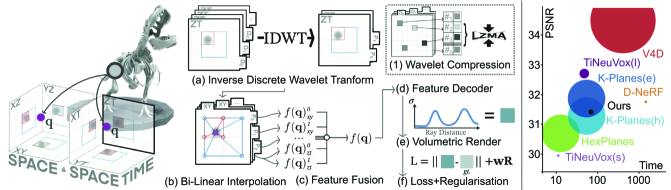
Figure 1: Method overview. We represent N-level wavelet coefficients as $\mathbf{\Omega}^{s}_{c}$. (a) The wavelet representation is transformed using the inverse discrete wavelet transform (IDWT). (b) 4-D samples are projected onto each plane and bi-linearly interpolated over multiple scales. (c) Features sampled from different planes and multiple scales are fused into a single feature. (d) Features are linearly decoded. (e) A 2-D pixel is rendered from the 3-D volume using the NeRF volumetric rendering function. (f) A loss and weighted regularization is used for training. After training: (1) We compress non-zero wavelet coefficients. Model Comparison: Our model is small, fast and performant. Time is measured in minutes and model size is represented by point radius.

1 Introduction

Neural Radiance Fields (NeRFs) have gained significant attention due to their ability to generate high-resolution 3D scenes with accurate novel view synthesis. The traditional NeRF is designed for static scenes and struggles to model objects and scenes with motion. Dynamic NeRFs extend these capabilities to address this issue, broadening applications in computer graphics by supporting the generation of realistic object and scene animations. While static NeRF frameworks yield impressive results, dynamic NeRF frameworks still face numerous limitations, particularly associated with complexity, scalability and stream-ability.

Recent advancements in plane-based representations, including matrix-vector and plane decomposed 3-D space, have demonstrated promising results for static scenes [6, 24, 14]. These representations have also shown success in modelling dynamic environments [11, 4] and demonstrate substantial improvements to training speed. However, the significance and interpretability of the temporal component (represented by an axis on a 2-D feature planes) have not been fully realized, particularly in scenarios with high spatial detail or fast motion. Consequently, these models tend to be large and challenging to compress, making tasks such as 4-D video streaming problematic. For static scenes, wavelet-based plane representations have been used to alleviate these problems [21]. However this approach has not been explored for dynamic scenes.

In this paper, we propose the use of wavelets as a basis for a 4-D decomposed plane representation, as demonstrated in Figure WavePlanes: A compact Wavelet representation for Dynamic Neural Radiance Fields. Our motivation is to provide a highly compressible representation, which could benefit data-intensive transmission tasks such as 4-D video streaming.

Two design choices are proposed to improve the processing time, performance and final model size:

• Firstly, we shift the reconstructed space-time features by +1, prior to feature fusion. This maximizes the likely hood of static empty space represented by the fused features while preserving sparsity in the decomposed wavelet representation. This consequently enables our proposed wavelet-based compression scheme.

• Secondly, we offer modifications to previously proposed time smoothness and time sparsity (TS) regularizers in [11]. Substituting the time smoothness regularizer, we propose smoothing spatial features on the space-time planes. This improves performance on scenes with rapid changes in motion. We also modify the time sparsity function to work directly on the wavelet coefficient representation. This eliminates the need for signal reconstruction during regularization and noticeably reduces the training time.

The proposed compression scheme (Figure WavePlanes: A compact Wavelet representation for Dynamic Neural Radiance Fields (1)) exploits the sparsity of our representation to further reduce our model size without using an MLP and without affecting performance. This is accomplished by filtering the wavelet coefficients using hard thresholding, constructing a Hash Map containing non-zero coefficients and their locations on each wavelet plane, and then compressing it using a lossless algorithm.

Finally, we investigate alternative feature fusion methods (Figure WavePlanes: A compact Wavelet representation for Dynamic Neural Radiance Fields (c)), and its relevance to model interpretability. Up to this point, only the element-wise feature factorization and addition were tested [11]. Hence, we extend the investigation and propose two feature fusion methods capable of competing with the prior factorization-only scheme while offering better interpretability.

In summary, we contribute:

1. A wavelet-based plane representation for modelling dynamic scenes as explicit 4-D volumes; offering a compressible and fast model capable of competing with the state-of-the-art.

2. New regularizers for plane-based approaches.

3. A novel compression scheme that achieves state-of-the-art model size.

4. Alternative feature fusion schemes with more interpretability and comparable performance to prior schemes.

2 Related Work

Dynamic NeRFs.

Representing 3-D volumes in time is currently accomplished by one of the following techniques:

1. Jointly learning a 3-D “canonical” (static) and 3-D deformation field. This anchors the canonical field to a point in time, typically $t=0$s, where the deformation field linearly shifts canonical field volumes in space, conditioned on time, as proposed in D-NeRF [20] and Dy-NeRF [15]. It disentangles time-conditioned spatial features in a way that preserves volumetric consistency. However, they are not capable of discovering view-dependant effects under motion. NeRF-DS [30] addresses this by conditioning color features on surface position and orientation. Unfortunately, this approach still fails to adapt to temporal changes in scene topology.

2. Decomposing 4-D into representational components, such as matrix-vectors and planes. This approach was introduced by Tensor4D [23], which offers a 9-plane candecomp/parafac [5, 13] /matrix-matrix (MM) decomposition. Subsequently, K-Planes [11] and HexPlanes [4] proposed a 6-plane and 6-plane+6-vector decomposition, respectively, along with various feature-plane fusion schemes. HexPlanes uses a multiplicative-additive approach similar to Tensor4D, while K-Planes demonstrates that a purely multiplicative approach is preferred over an additive approach.

3. Using static representations as a set of key-frames. This approach relies on the robustness and compactness of static NeRF representations, along with the effectiveness of a key-frame interpolation strategy. NeRFPlayer [25] decomposes features into static, deforming and “new areas”, where the latter is used to represent temporal changes that occur after the first key frame, such as water gradually mixing with coffee. HyperReel [1] proposes a hierarchical key-frame interpolation strategy that is compact and fast as a result of using TensoRF [6] for modelling each key-frame. However, it is limited by computational requirements needed to load the model. There is also an overlap with approach (2), as HumanRF [14] utilizes a key-framed MM decomposition for dynamic human modelling; storing and selecting a set of space-only (static) feature planes for at each time frame.

4. Directly learning a 4-D field conditioned on time. This groups the remaining work. DynIBaR [16] proposes a novel ray-conditioning scheme for dynamic videos, where features in each frame are conditioned on the predicted features of surrounding frames. V4D [12] proposes a texture driven, time-conditioned, voxel-based model where pixel-level refinement and a conditional positional encoder are used to handle over-smoothing caused by the total variation regularizer.

Each approach has its own set of benefits and drawbacks. For instance, using MLPs results in small models size but long optimization times. Whereas explicit approaches, such as K-Planes, offer faster optimization though require significantly more storage, as indicated in Figure WavePlanes: A compact Wavelet representation for Dynamic Neural Radiance Fields. As a plane-based approach our method is fast, yet we are not limited by model size.

Wavelet NeRFs.

Using wavelets to model static scenes is a recent development and has demonstrated the ability to enhance the compactness of existing representations [22, 21, 29]. WIRE [22] proposes better-suited activation functions for implicit neural representations and achieves a reduction of $p/\sqrt{2}$ w.r.t the number of trainable parameters by proposing a complex Gabor wavelet activation. The authors in [21] propose a tri-plane decomposed wavelet-based representation. To improve compression, an additional mask for each plane is learnt to exploit the sparsity of the tri-plane representation, which reduces the model size to around 2MB. We have yet to see this applied to modelling dynamic scenes. Hence, in this paper we introduce the first wavelet-based approach for modelling 4-D volumes.

K=4-Planes Background.

We extend the K-Planes (explicit) model, which learns 4-D feature volumes in space and time, $f(\mathbf{q})$ where $\mathbf{q}=(x,y,z,t)$, as a set of multi-scale 2-D feature planes, $\mathbf{P}^{s}_{c}$ for $c\in C=[xy,xz,yz,xt,yt,zt]$ and $s\in S=[64,128,256,512]$ with a constant scale for time. To sample features, $\mathbf{q}$ is normalized and projected onto each plane using $f_{c}(\textbf{q})=\psi(\textbf{P}_{c},\pi_{c}(\textbf{q}))$, where $\pi_{c}$ denotes the planar projection and $\psi$ denotes the bi-linear interpolation of the projected point on a 2-D grid. Subsequently a 4-D feature volume is reconstructed using the Hardman Product (HP) (an element-wise operator), in Equation 1.

$$f(\mathbf{q})=\llbracket\prod_{c\in C}f_{c}^{s}(\mathbf{q})\rrbracket^{s\in S}$$ (1)

Where $\prod$ applies the HP operator fusing plane features and $\llbracket\cdot\rrbracket$ represents a concatenation across scales.

The space-time planes, denoted as $c_{t}\in C_{t}=[xt,yt,zt]$, are initialized and regularized towards 1. This provides some interpretability as it allows the separation of static components where $f_{c_{t}}(\textbf{q})=1$, representing the multiplicative-1 identity in Equation 1. Still, the case where $f_{c}(\textbf{q})=0$, representing the multiplicative-0 identity, is not considered. The influence of a zero-valued feature in Equation 1 is globally destructive and is interpreted differently for space-only and space-time planes. zero-valued space-only features indicate empty static space and zero-valued space-time features identify empty static slices of 3-D space at a given time, as illustrated in Figure 2. Hence, our intention is to explore alternative approaches to HP feature fusion that avoid the destructive result of zero-valued features to offer a higher level of interpretability.

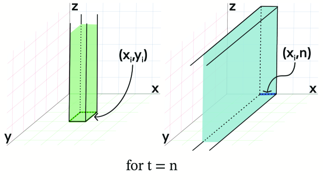
Figure 2: The volumetric regions at time $t=n$ affected by a single feature on $P_{xy}$ (a tile) and $P_{xt}$ (an edge), respectively; for the HP fusion scheme.

3 WavePlanes

In WavePlanes, the representation is stored as a set of 2-D wavelet coefficients, $\mathbf{\Omega}^{s}_{c}$ and is encoded using the IDWT into a fine and a coarse feature plane, $P_{c}^{0}$ and $P_{c}^{1}$, as shown in Figure WavePlanes: A compact Wavelet representation for Dynamic Neural Radiance Fields (a). This is accomplished by performing the IDWT twice with the full set and a reduced set of wavelet coefficients, respectively. Note that we use $s\in[0,1,...,N]$ to indicate the level of a wavelet plane rather than the scale of a feature plane.

3.1 Feature Plane Reconstruction

We refer to the father wavelet coefficients as $\Omega_{c}^{[s=0]}\in\mathcal{R}^{B\times H/2^{N}\times W/2^{N}}$, where $B$ is the feature length, $(H,W)$ is the desired height and width of the reconstructed feature plane and $2^{N}$ is a down-sampling factor involved in wavelet decomposition. The mother wavelet coefficients are defined as $\Omega_{c}^{[s>0]}\in\mathcal{R}^{B\times 3\times H/s^{\prime}\times W/s^{\prime}}$, where 3 indicates the number of filters and $s^{\prime}=2^{N-s}$ allows for down-sampling where the highest frequency signal will have size $(H/2,W/2)$ and the lowest frequency will have size $(H/2^{N},W/2^{N})$. Hence, for a wavelet decomposition level of 2, $N=2$ and $s\in[0,1,2]$.

To avoid vanishing gradients for high-frequency coefficients during the IDWT, we apply the frequency-based scaling factor to each plane, denoted by $\mathbf{k}\odot\mathbf{\Omega}_{c}$ where $\mathbf{k}=[1,\frac{2}{5},\frac{1}{5}]$ as suggested in [21]. Note that we select smaller values.

To reconstruct the feature planes we use Equation 2. Using a 2-level decomposition, we find that producing two scales of features for $s=1$ and $s=2$ is sufficient.

$$P_{c}^{s}(\Omega_{c}|s)\begin{cases}\text{IDWT}(\mathbf{k}\odot\Omega_{c}^{[0:s]}),&\text{if }c\in[xy,xz,yz]\\ \text{IDWT}(\mathbf{k}\odot\Omega_{c}^{[0:s]})+1,&\text{otherwise}\end{cases}$$ (2)

Where the $+1$ term shifts the space-time features towards 1. This preserves sparsity in the wavelet representation as coefficients are naturally biased towards 0. This biases the feature representation toward 1, providing separability between static and dynamic volumes [11].

3.2 Feature Fusion and Interpretability

Following K-Planes, a 4-D sample, $\mathbf{q}$, is normalized between $[0,S)$, projected onto each plane and bi-linearly interpolated using $f(\mathbf{q})_{c}^{s}=\psi(\mathbf{P}_{c}^{s},\pi_{c}(\mathbf{q}))$, where $\psi$ and $\pi_{c}$ were discussed in Section 2. Consequently we can obtain a HP-fused feature using Equation 1.

The feature fusion process allows us to interpret space-only planes as a set of localized features that are transformed by any element-wise operator using features from the space-time planes. This implies that the HP operator is used to constrain the time at which a spatial volume becomes static, i.e. when $f_{c_{t}}(\mathbf{q})=1$. As previously mentioned, the issue when $f_{c}(\mathbf{q})=0$ has been (unknowingly) addressed in K-Planes through the introduction of the sparse transients regularizer, which biases features towards 1. In our case, we relax the weighting for this regularizer and introduce a new factorization scheme that achieves similar benefit by instead conditioning the multiplicative-0 identity in an attempt to increase the rendering quality for occluded regions of empty space - a challenge for the original K-Planes model. We propose two schemes below.

Zero-agreement masked multiplication (ZMM).

We first develop the HP fusion scheme, where all zero-valued space-time features for a 4-D volume sample are conditioned to agree on empty dynamic space. If the temporal features of a given sample are not all zero-valued then the zero-valued features are treated as 1-valued features, allowing gradient flow without modifying the fused feature. We express this as a differentiable binary mask, $Q_{c}(\cdot)$, where 1 indicates zero-valued inputs. We replace all zero-valued features in $f_{c_{t}}(\mathbf{q})$ with 1 and perform the feature factorization only across the space-time planes as shown in Equation 3. Using Equation 4 we subsequently recover an inverted binarized mask that is multiplied by the new space-time features as in Equation 5. Finally, the result is multiplied with feature samples from the space-only planes to recover a 4-D feature volume.

$$f_{c_{t}}^{{}^{\prime}}(\mathbf{q})=f_{c_{t}}(\mathbf{q})+Q_{c_{t}}(f_{c_{t}}(\mathbf{q}))$$ (3)

$$Q^{-1}=|\mathbf{1}-\prod_{c\in C_{t}}Q_{c}(f_{c}(\mathbf{q}))|$$ (4)

$$f_{\text{space-time}}(\mathbf{q})=Q^{-1}\cdot\prod_{c\in C_{t}}f_{c}^{{}^{\prime}}(\mathbf{q})$$ (5)

Hence, the volume sample becomes empty only when all space-time features for a 4-D sample agree on a zero-value.

Zero-agreement masked addition (ZAM).

A natural interpretation of the zero-agreement condition in ZMM is the addition of space-time features only. This is implemented using Equation 6, where a sum of 0 results in the multiplicative-0 identity and the $1/3$ factor ensures that when all space-time features are 1 the sum is also 1, retaining the separability of static and dynamic volumes. Therefore temporally dependant static volumes are still represented by $f_{c}(\mathbf{q})=1$ and empty space is naturally represented by $f(\mathbf{q})=0$.

$$f(\mathbf{q})=\llbracket\frac{1}{3}\sum_{c\in C_{t}}f_{c}^{s}(\mathbf{q})\cdot\prod_{c\in C}f_{c}^{s}(\mathbf{q})\rrbracket^{s\in S}$$ (6)

3.3 Compressing Wavelets with Hash Maps

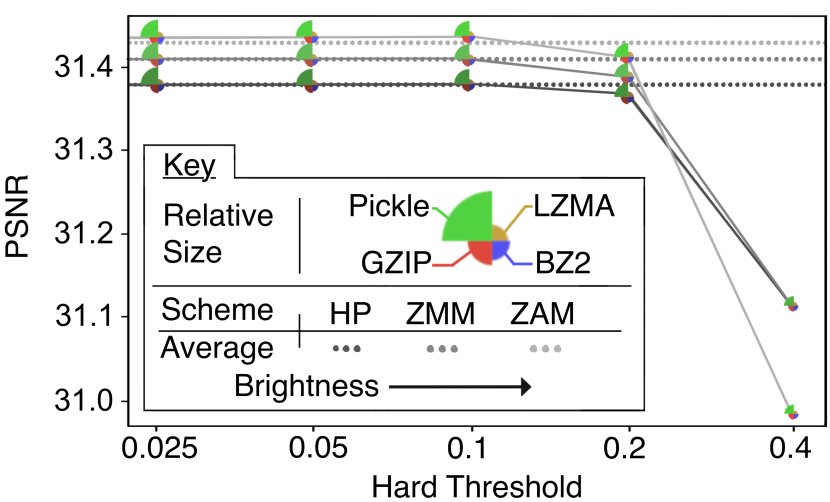
Figure 3: Evaluating Pickle, GZIP, Burrow-Wheeler (BZ2) and Lempel–Ziv–Markov chain (LZMA) compression algorithms on the proposed feature fusion schemes, using the D-NeRF T-Rex scene [20]. The model size produced by each compression scheme is represented by the radius of corresponding slice.

A benefit of using wavelets is the ability to compress representations by relying on the tendency of coefficients to be zero. Unlike other plane-based models, this is true for all of our planes and is possible thanks to the condition proposed in Equation 2. We apply compression with Hash Maps after training and demonstrate in Figure 3 the size difference with various lossless compression schemes. Using Hash Maps means our representation can be rapidly reconstructed with $O(1)$ time complexity.

Before compression, we apply hard thresholding to each coefficient on each grid-plane $\mathbf{\Omega}_{c}$. As we model features and not signals, the significance of non-zero coefficients is ambiguous. Still, the feature landscape is smooth and zero-valued coefficients are not ambiguous, so we can filter near-zero coefficients without deprecation.

We then use a Hash Map to store all non-zero values where each key states the value’s location within the set $\mathbf{\Omega}_{c}$. For most planes this results in (approximately) a 90% reduction of the the number of values to be stored. The only case for which this is not true is for space-only father-wavelets planes, where we observe only a $<1\%$ reduction, indicating that data is concentrated on these planes.

We select the appropriate threshold value and lossless compression algorithm using Figure 3, where LZMA and a threshold of $0.1$ produce the smallest model size without loss. As compression is lossless, the small improvements in PSNR for the ZAM results indicate some denoising capability linked to hard-thresholding. This could be explored in future work for denoising non-zero features distributed around means, potentially indicating material classes.

3.4 Optimization

Regularization.

For dynamic scenes, we use three regularizers, namely total variation (TV), spatial smoothness in time (SST) and TS. TV regularization was used for static scenes in Plenoxels [10] and TensoRF [6] and recently for dynamic scenes in K-Planes. This is defined in Equation 7.

$$\mathcal{L}_{TV}(\mathbf{P})=\frac{1}{|C|n^{2}}\sum_{c,i,j}(||\mathbf{P}^{i,j}_{c}-\mathbf{P}^{i-1,j}_{c}||^{2}_{2}+||\mathbf{P}^{i,j}_{c}-\mathbf{P}^{i,j-1}_{c}||^{2}_{2})$$ (7)

The proposed SST regularizer is denoted in Equation 8 and represents the 1-D Laplacian approximation of the second derivatives of the spatial components for each time-plane. Rather than smoothing along the time-axis, as is done in K-Planes, we find that smoothing spatial components produces better results. Please refer to the supplementary materials for an ablation study.

$$\mathcal{L}_{SST}=\frac{1}{|C|n^{2}}\sum_{c,i,t}\mathbf{P}^{i-1,t}_{c}-2\mathbf{P}^{i,t}_{c}+\mathbf{P}^{i+1,t}_{c}||^{2}_{2}$$ (8)

TS regularization is proposed in Equation 9 and maximizes the number of zero-valued space-time wavelet coefficients. This pairs well with our compression scheme as it directly maximizes the sparsity of $\mathbf{\Omega}_{c_{t}}$.

$$\mathcal{L}_{TS}=\sum_{c_{t}\in C_{t}}||\mathbf{\Omega}_{c_{t}}||_{1}$$ (9)

Feature decoder with learned color basis.

We treat fused features as coefficients of spherical harmonics (SH) basis. SH has been used in Plenoctrees [31], Plenoxels and TensoRF for static scenes and was recently used in [26] for modelling scenes as Fourier Plenoctrees. The degree of the SH often leads to limited expressivity. This suggests a trade-off between high computational cost and sensitive convergence for higher levels of expressivity. Instead, NeX [28] uses a per-scene learned color basis, where features are treated as coefficients for a linear decoder. K-Planes demonstrates this for dynamic scenes so we utilize the same approach where a basis is learnt using a tiny fully-fused MLP [19]. This maps the viewing direction $\mathbf{d}$ to red, green and blue basis vectors, $b_{i}(\mathbf{d})$ for $i\in\{R,G,B\}$. An additional density basis is learnt and left independent of viewing direction. Subsequently, color and density values are recovered by applying the dot product between basis vectors $b_{i}(\mathbf{d})$ and fused features $f(\mathbf{q})$.

Proposal Sampling Network.

Mip-NeRF 360 [3] introduced proposal sampling as an iterable method with $n_{p}$ stages. At each stage a network roughly predicts spatial density at a given time to infer regions of interest - higher density regions are sampled more frequently. For each stage we have the option to re-use the original proposal network or instantiate additional proposal networks. We chose two stages for the proposal sampling scheme and as it incurs minimal cost we use different proposal networks at each iteration with feature length 8 and 16, respectively. We use a lower resolution version of our model as the proposal network. Finally, the proposal networks are trained using a histogram loss [3].

Importance Sampling

based on temporal differences (IST) is proposed in DyNeRF [15] to handle the real dynamic DyNeRF data set. Rays are sampled in relation to their maximum color variance, thus higher sampling is attributed to 4-D volumes that are assumed to be dynamic. In our experiments, we follow the same strategy proposed in K-Planes, whereby we sample rays uniformly for the first half of training and then apply the IST strategy.

3.5 Implementation

Our implementation is a branch off the K-Planes repository. To implement the wavelet functionality we use the pytorch_wavelets library [7]. To boost training speed we cache (on the GPU) the resulting feature planes, $\mathbf{P}_{c}^{s}$, at the start of every epoch to avoid re-processing the IDWT during regularization. This significantly reduces training time though increases memory consumption, shown in Table 1. The memory footprint for the faster approach is larger than K-Planes yet GPU utilization is lower. This is important as utilization ultimately limits our ability to run K-Planes on larger data sets with our available hardware.

Method	Mem. $\downarrow$	Util. $\downarrow$	Time $\downarrow$
D-NeRF data set [20]
K-Planes [11]	7.0 GB	86%	59 mins
Ours	7.7 GB	79%	72 mins
Ours without Caching	7.4 GB	70%	120mins
DyNeRF data set [15]
K-Planes* [11]	-	-	-
Ours	9.7 GB	89%	510mins
Ours without Caching	9.1 GB	82%	690mins

Table 1: Computational comparisons of our model with and without caching the wavelet representation. Further comparison with K-Planes is provided and both models use HP fusion for fair comparison. Mem. is the GPU memory. Util. is the GPU utilization. Time is the training time. *Did not run on our hardware.

y

4 Results

We employ a 4k batch size and the same scene bounding boxes used in [11] for fair comparison. For synthetic scenes we select a spatial resolution of $H=W=256$ for high-complexity scenes and 128 for low-complexity scenes. This reduces memory consumption and training time while producing comparable results, in contrast to other models which usually select resolutions up to 512. Additionally, for all experiments, we evaluate our ZMM-based approach with feature length $B=64$, using PSNR and SSIM, as shown in Table 2. Quantitative (objective metric) results for the ZAM and HP approaches are provided in the supplementary materials and show similar performance. Note that we did not retrain the existing models; all results were taken from the original papers. In the ablation study, we further separate the PSNR evaluation for foreground and background renders. This reduces ambiguity in image-quality assessment metrics, which can exhibit bias towards large white backgrounds for synthetic scenes. The foreground and background are using the alpha mask of RGBA image data sets. Then morphological dilation is applied to include noisy foreground artifacts in foreground evaluations.

We are limited by access to high-performance compute systems and all tests were carried out on a 24GB NVIDIA RTX 3090 GPU. For LLFF and D-NeRF data sets we used 32GB of RAM whereas DyNeRF required 98GB of RAM. For most data sets this is not an issue. However, for the DyNeRF data set [15] we are unable to pre-generate IST weights with the usual 2$\times$ down sampling. Hence, we choose to down sample by 8$\times$ during IST weight generation and 2$\times$ during training, to demonstrate our model’s ability to synthesize real dynamic scenes.

	PSNR $\uparrow$		SSIM $\uparrow$	# Params $\downarrow$	Average Size $\downarrow$
	Full	Partial
Real static LLFF scenes [17]
Plenoxels [10]	26.29	28.84	0.839	$\sim$500M	-
Masked Wavelets (small) [21]	26.25	29.05	0.839	-	3.2MB
Masked Wavelets (large) [21]	26.54	29.42	0.839	-	7.4MB
K-Planes (explicit) [11]	26.78	29.75	0.847	19M	$\sim$ 100MB
Ours	26.10	29.30	0.825	51M	93MB
Real dynamic DyNeRF scenes [15]
HexPlanes [4]	31.71	-	-	-	$\sim$ 200MB
K-Planes (explicit) [11]	31.30	-	0.960	51M	250MB
K-Planes (hybrid) [11]	31.92	-	0.964	27M	250MB
Ours	29.75	-	0.922	67M	58MB
Synthetic dynamic D-NeRF assets [20]
D-NeRF [20]	29.67	26.14	0.95	1-3M	13MB
V4D [12]	33.72	29.06	0.98	275M	377MB
TiNeuVox-S [9]	30.75	27.10	0.96	-	8MB
TiNeuVox-B [9]	32.67	28.63	0.97	-	48MB
HexPlanes [4]	31.04	27.50	-	-	$\sim$ 200MB
K-Planes (explicit) [11]	31.05	27.45	0.97	37M	$\sim$ 200MB
K-Planes (hybrid) [11]	31.61	27.66	0.97	37M	$\sim$ 200MB
Ours	30.50	27.43	0.97	16M	12MB

Table 2: Average novel view synthesis results. Partial indicates a subset of the data set.

4.1 Real Static Scenes

We assess WavePlanes on the sparse, forward-facing, bounded, multi-view and real static LLFF data set [17]. Each scene contains 20-60 images and is down sampled to 1008$\times$756 pixels. In this experiment WavePlanes is reduced to a tri-plane model, using HP fusion. While it performs satisfactorily over the full data set, WavePlanes demonstrates competitive performance on scenes containing $>$35 training images, indicated by the partial results in Table 2. Visually, we find that WavePlanes is better at dealing with edges and is capable of modelling complex features, e.g. the rib-cage in Figure 4.

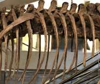
(a) Ours

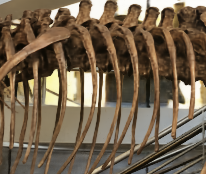
(b) K-Planes

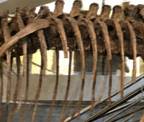
(c) TensoRF

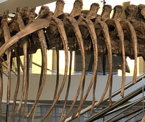
(d) Ground Truth

Figure 4: Zoomed visual comparison of real static scene renders. Demonstrating WavePlanes ability to model static scenes.

4.2 Dynamic Scenes

Real multi-view scenes.

The DyNeRF data set [15] is used to test our model’s ability to perform novel view synthesis on forward-facing, multi-view (19-21 cameras), real dynamic scenes lasting 10 seconds at 30FPS. The scenes contain different indoor lighting set-ups with a large variation of textures and materials. For this test, we use a temporal resolution of $W=150$. Quantitative results in Table 2 indicate desirable performance for our method, considering the reduced quality of the sampling strategy. Visually, WavePlanes performs novel view synthesis well and shows sharper edges and less noise on a number of objects in the scene, e.g. the pattern on the uncooked salmon is clearer whilst those of K-Planes are smoothed out, shown in Figure 5. This is notably accomplished with a memory budget at least 4$\times$ smaller than other plane-based methods.

Ours*	K-Planes (explicit)*	K-Planes (hybrid)*	HexPlanes	DyNeRF	Ground truth

Figure 5: Qualitative real video results. WavePlanes can synthesize real objects to an acceptable standard. *Trained on the first 10/40 seconds.

Synthetic monocular scenes.

The D-NeRF data set [20] was used to perform novel view synthesis on low and high complexity synthetic object animations. These were captured using monocular “teleporting” cameras rotated at 360^∘ and contain 50-200 training frames that are down sampled to 400$\times$400 pixels. For this experiment, the resolution of the time axis for space-time grids is equivalent to the number of training images. WavePlanes performs adequately across the entire data set and particularly well on scenes containing a high amount of occlusion while being compact and small in size. This is indicated by the partial results in Table 2 that comprises the Lego, T-Rex and Hell Warrior scenes. The visual results in Figure 6 shows that WavePlanes achieves cleaner results than K-Planes and produces better detail in high frequency areas than K-Planes and TiNeuVox, e.g. around the T-Rex’s mouth. For Hook-D-NeRF scene, our method smooths high-frequency errors found in the K-Planes making the visual result more comprehensible, e.g., the mouth guard and shoulder of the Hook character.

(a) Ours

(b) K-Planes

(c) TiNeuVox

(d) Ground Truth

Figure 6: Visual comparison of the T-Rex and Hook D-NeRF scenes [20] (Success and Failure case). WavePlanes can produce better results for high occlusion scenes (T-Rex). Even for the failure case WavePlanes is less noisy than K-Planes (Hook).

4.3 Feature Fusion.

Results provided in Table 3 and Figure 7 demonstrate the effectiveness of the proposed feature fusion schemes on the D-NeRF data set. ZMM and ZAM are capable of outperforming other plane-based models for synthetic scenes. Despite the difference in IST down sampling, ZAM provides decent objective results for the real scene. Visually, we notice a slightly smoother render with higher attention to contrast for the ZMM approach.

	PSNR $\uparrow$			SSIM $\uparrow$	Time $\downarrow$
	Whole	Front	Back
T-Rex (synthetic) D-NeRF [20]
K-P	31.28	-	-	0.980	58min
HexP.	30.67	-	-	-	11min
HP	31.38	20.71	75.66	0.978	72min
ZMM	31.41	20.74	76.41	0.978	78min
ZAM	31.43	20.77	77.11	0.979	76min
Flame Salmon (real) DyNeRF [15]
K-P.	28.71	-	-	0.942	222min
HexP.	29.47	-	-	-	720min
HP	27.31	-	-	0.893	510min
ZMM	27.6	-	-	0.893	540min
ZAM	28.25	-	-	0.900	530min

Table 3: Quantitative results for propose feature fusion schemes. We compare quality and training time to other plane-based models. K-P and HexP. are the K-Planes (explicit) and HexPlanes+ results, respectively.

HP	ZAM	ZMM	Ground Truth

Figure 7: Qualitative feature fusion results. Differences can be seen in the amount of noise and around the left leg and the hip.

4.4 Ablation Study

We perform an ablation study using the D-NeRF synthetic data set [20]. Please refer to the supplementary materials for more results.

Wavelet family.

Table 4 compares different wavelet functions with varying degrees of regularity. Regularity indicates the number of continuous derivatives that wavelet function has and is tied to the number of vanishing moments, denoted by the $M$ in “dbM”, “coifM”, etc. For wavelets with less regularity (e.g. the Haar wavelet) we find our method performs worse on foreground predictions. Wavelets with higher regularity are also negligibly slower. However, we find the coif4 wavelet is an exception as it is performant yet slightly slower (by $\sim 5$minutes). This is likely because it has a larger filter length, of $6M$, compared with other functions such as dbM with length $2M$. Overall, the results indicate that orthogonality and symmetry have little importance, whereas the function’s shape, regularity and filter length impacts performance the most. Similar conclusions were found for low-bit rate wavelet coding tasks [8], which may suggest that this is shared characteristic of low-resolution image tasks, such modelling dynamic scenes using low resolution (400$\times$400 pixel) images.

	PSNR $\uparrow$			SSIM $\uparrow$
	Whole	Front	Back
Wavelet families
Haar	30.85	20.18	75.58	0.977
Coif2	31.06	20.38	77.01	0.977
Coif4	31.10	20.43	78.45	0.977
Bior1.3	30.99	20.31	77.98	0.977
Bior4.4	31.12	20.45	75.41	0.977
Db2	31.00	20.33	77.58	0.977
Db6	31.08	20.42	76.62	0.977
$N$-Level Wavelet
2	31.30	20.63	76.01	0.977
3	30.46	19.79	74.08	0.975
4	30.22	19.56	69.29	0.974

Table 4: Wavelet families: Comparing the quality of different wavelet functions. $N$-Level Wavelet: Comparing varying levels of wavelet decomposition.

Wavelet decomposition level.

In Table 4 we compare the number of wavelet levels for the main WavePlane field. More levels of decomposition means more coefficients, which in turn impacts performance and rendering time significantly. The convergence of higher levels of wavelet decomposition is also slower where a 2-level decomposition is $\sim 13$ minutes faster than a 3-level decomposition.

5 Conclusion and Future Work

Conclusion.

We propose WavePlanes, the first wavelet-based approach for modelling dynamic NeRFs. We show that our model can synthesize various scenes without the need for high performance computing resources or custom CUDA code, while producing competitive objective results and perceptually pleasing visual results. By exploiting the characteristics of the wavelet representation, our novel compression scheme reduces the final model size by up to 15$\times$ compared to other plane-based models without significantly impacting training time or performance.

Future work.

Plane-based approaches are currently limited in their ability to model objects outside of the predefined bounding box [23, 21, 11]. In future work it could prove beneficial to model the out-of-bounds scene with a HDRI-style mapping, similar to what was proposed for NeRF++ [32].

Additionally, using discrete grids with a fixed temporal resolution makes it challenging to model fast motion without introducing some degree of temporal uncertainty (noise). This limitation is shared by current dynamic plane-based models. However, the results from our compression scheme indicate that the high pass filter applied to our wavelet representation may be useful for denoising. Consequently, a more sophisticated approach could be explored to correct regions of space-time affected by high motion noise. For instance, by classifying wavelet features a band pass filter could be used to contract features dispersed around a class means. Filtering non-zero coefficients would also lead to better compression as more values would be repeated. This may alleviate limitations in our compression scheme when a scene contains little empty space, as is the case for numerous LLFF scenes.

Appendix A NeRF Background

Rendering Equation.

Given set of color and density samples, $\mathbf{c}$ and $\mathbf{\sigma}$, indexed by $i$ along a ray, we use the same equation as in NeRF [18], Equation 10, to render each pixel of a novel view.

$$C=\sum_{i=1}^{N}\text{exp}(-\sum_{j=1}^{i-1}\sigma_{j}\delta_{j})(1-\text{exp}(\sigma_{i}\delta_{i}))\mathbf{c}_{i},$$ (10)

where $\delta_{i}$ is the width of a volumetric sample along a ray, the first exponential represents the transmittance of sample $i$ w.r.t. earlier samples along a ray, and the second term, 1-exp($\cdot$), is the absorption of the sample. Combined, these model the contribution of each color sample along a ray, the sum of which approximates the color of each pixel.

Appendix B Additional Hyper Parameters

All configuration files are provided with our code: https://github.com/azzarelli/waveplanes/. For all experiments we use cosine annealing with a brief linearly increasing warm-up (512 steps) as our learning function. The notable differences between experiments are:

1. For the LLFF data set [17] we use 4x down sampling, with normalized device coordinates, a learning rate of $0.02$, a 4-layer linear feature decoder and $40$k training steps. All LLFF experiments share the same configuration file.

2. For the real DyNeRF data set [15] we use 8x down sampling to generate the IST weights and 2x down sampling to train the model for $120$k steps with a learning rate of $0.01$. All DyNeRF experiments share the same configuration file, however we find that the ZMM and ZAM fusion schemes work better with a 3-layer and 4-layer linear feature decoder, respectively; demonstrated in Table 5.

3. For the synthetic D-NeRF data set [20] we use 2x down sampling, normalized device coordinates and a learning rate of $0.01$ for $30$k training steps. For this experiment, we tune our model per-scene. Individual configuration files have been made available and differ in resolution, as discussed in the paper.

Scheme	# Layers	PSNR $\uparrow$	SSIM $\uparrow$
Coffee Martini Scene
ZMM	3	27.40	0.8767
ZMM	4	25.80	0.8733
ZAM	3	27.51	0.8832
ZAM	4	27.17	0.8854
Flame Steak Scene
ZMM	3	30.40	0.9271
ZMM	4	30.31	0.9312
ZAM	3	28.67	0.9312
ZAM	4	30.49	0.9331

Table 5: Comparing 3 and 4 layered linear feature decoders for the ZMM and ZAM fusion schemes on DyNeRF scenes.

Appendix C Additional Results

C.1 Per-Scene Results

Real static scenes.

In Table 6 we compare our model with the state-of-the-art, including the masked wavelet representation [21], for the LLFF data set. We also evaluate our model with feature length $B=$32 and 64. With $B=$32 the model consists of 27M parameters and trains in just over 1 hour, whereas a feature length of 64 uses 51M parameters and trains in under 2 hours. We selected $B=64$ for our main experiment as it provides better quantitative and qualitative results. In Figure 8 we provide visual examples of LLFF scenes modelled with WavePlanes.

PSNR $\uparrow$
	Room	Fern	Leaves	Fortress	Orchids	Flower	T-Rex	Horns	Means
NeRF	32.64	25.17	20.92	31.16	20.36	27.40	26.80	27.45	26.50
Plenoxels [10]	30.22	25.46	21.41	31.09	20.24	27.83	26.48	27.58	26.29
TensoRF (large) [6]	32.35	25.27	21.30	31.36	19.87	28.60	26.97	28.14	26.73
Masked Wavelets* (small) [21]	31.19	25.05	21.08	30.75	19.76	27.94	26.77	27.48	26.25
Masked Wavelets* (large) [21]	31.73	25.27	21.17	31.01	20.02	28.20	27.07	27.88	26.54
K-Planes (explicit) [11]	32.72	24.87	21.07	31.34	19.89	28.37	27.54	28.40	26.78
K-Planes (hybrid) [11]	32.64	25.38	21.30	30.44	20.26	28.67	28.01	28.63	26.92
Ours-64	31.47	23.89	20.90	30.36	19.21	27.61	27.02	28.33	26.10
Ours-32	31.29	23.99	21.03	30.08	19.41	26.08	26.80	28.00	25.84
SSIM $\uparrow$
NeRF	0.948	0.792	0.690	0.881	0.641	0.827	0.880	0.828	0.811
Plenoxels [10]	0.937	0.832	0.760	0.885	0.687	0.862	0.890	0.857	0.839
TensoRF (large) [6]	0.952	0.814	0.752	0.897	0.649	0.871	0.900	0.877	0.839
K-Planes (explicit) [11]	0.955	0.809	0.738	0.898	0.655	0.867	0.909	0.884	0.841
K-Planes (hybrid) [11]	0.957	0.828	0.746	0.890	0.676	0.872	0.915	0.892	0.847
Ours-64	0.9492	0.7762	0.7277	0.8934	0.6277	0.8392	0.8989	0.8856	0.8247
Ours-32	0.9453	0.7694	0.7354	0.8838	0.6320	0.8108	0.8905	0.8725	0.8175

Table 6: Quantitative results from the real LLFF data set [17]. We evaluate our 3-D model with feature length 32 and 64. *SSIM results are not provided.

Leaves	Fern	Orchids	Flower
T-Rex	Horns	Fortress	Room

Figure 8: Visual results from the LLFF data set [17].

Real dynamic scenes.

In Table 7 we breakdown the results from each scene in the DyNeRF data set to provide a quantitative comparison the HP, ZMM and ZAM feature fusion schemes. In Figure 9 we provide visual examples these scenes modeled with WavePlanes using the ZAM fusion scheme.

PSNR $\uparrow$
	Coffee	Spinach	Cut	Flame	Flame	Sear	Mean $\uparrow$
	Martini (CM)		Beef	Salmon	Steak	Steak	All	No CM
DyNeRF [15]	-	-	-	29.58	-	-	-	-
LLFF [17]	-	-	-	23.24	-	-	-	-
K-Planes (explicit)	28.74	32.19	31.93	28.71 **	31.80	31.89	30.88	31.30
K-Planes (hybrid)	29.99	32.60	31.82	30.44 **	32.38	32.52	31.63	31.92
HexPlane	-	32.042	32.545	29.470	32.080	32.085	-	31.71
HexPlane+	-	31.860	32.712	29.263	31.924	32.085	-	31.57
Ours-HP*	28.01	29.78	31.39	27.31	30.71	30.23	29.57	29.88
Ours-ZMM*	27.30	30.00	30.89	27.6	30.4	29.88	29.35	29.75
Ours-ZAM*	27.17	30.16	31.45	28.25	30.49	30.37	29.65	30.14
SSIM $\uparrow$
DyNeRF [15]	-	-	-	0.961	-	-	-	-
LLFF [17]	-	-	-	0.848	-	-	-	-
K-Planes (explicit)	0.943	0.968	0.965	0.942 **	0.970	0.971	0.960	-
K-Planes (hybrid)	0.953	0.966	0.966	0.953 **	0.970	0.974	0.964	-
Ours-HP*	0.8896	0.9191	0.9338	0.8928	0.9364	0.9271	0.9165	-
Ours-ZMM*	0.8767	0.9215	0.9258	0.8934	0.9271	0.9321	0.9145	-
Ours-ZAM*	0.8854	0.9235	0.9345	0.9001	0.9331	0.9385	0.9191	-

Table 7: Quantitative esults from the multi-view real DyNeRF dynamic scenes [15]. NoCM indicates mean without the Coffee Martini scene. * Uses 8x down sampling for IST weights. **K-Planes trains the Flame Salmon scene on the first 10 seconds of a 40 second clip.

Sear Steak	Flame Steak	Cut Beef
Coffee Martini	Cook Spinach	Flame Salmon

Figure 9: Visual results from the DyNeRF data set [15]. Using the ZAM feature fusion scheme.

Synthetic dynamic scenes.

In Table 8 we breakdown and compare the results from the D-NeRF data set for the HP, ZMM and ZAM fusion schemes. In Figure 10 we provide visual examples of each D-NeRF scene - rendered using ZAM fusion.

PSNR $\uparrow$
	Hell	Mutant	Hook	Balls	Lego	T-Rex	Stand-	Jumping	Mean $\uparrow$
	Warrior						Up	Jacks
D-NeRF	25.02	31.29	29.25	32.80	21.64	31.75	32.79	32.80	29.67
Tensor4D	-	-	-	-	26.71	-	36.32	34.43	-
TiNeuVox-S	27.00	31.09	29.30	39.05	24.35	29.95	32.89	32.33	30.75
TiNeuVox-B	28.17	33.61	31.45	40.73	25.02	32.70	35.43	34.23	32.67
V4D	27.03	36.27	31.04	42.67	25.62	34.53	37.20	35.36	33.72
K-Planes (explicit)	25.60	33.56	28.21	38.99	25.46	31.28	33.27	32.00	31.05
K-Planes (hybrid)	25.70	33.79	28.50	41.22	25.48	31.79	33.72	32.64	31.61
HexPlanes	24.24	33.79	28.71	39.69	25.22	30.67	34.36	31.65	31.04
Ours-HP	25.92	32.50	27.98	38.12	25.19	31.38	32.05	31.75	30.61
Ours-ZMM	25.63	32.51	27.97	37.71	25.26	31.41	32.15	31.33	30.50
Ours-ZAM	25.54	32.54	27.99	37.52	25.18	31.43	31.96	31.42	30.45
SSIM $\uparrow$
D-NeRF	0.95	0.97	0.96	0.98	0.83	0.97	0.98	0.98	0.95
Tensor4D	-	-	-	-	0.953	-	0.983	0.982	-
TiNeuVox-S	0.95	0.96	0.95	0.99	0.88	0.96	0.98	0.97	0.96
TiNeuVox-B	0.97	0.98	0.97	0.99	0.92	0.98	0.99	0.99	0.97
V4D	0.97	0.98	0.97	0.99	0.92	0.98	0.99	0.98	0.97
K-Planes (explicit)	0.951	0.982	0.951	0.989	0.947	0.980	0.980	0.974	0.969
K-Planes (hybrid)	0.952	0.983	0.954	0.992	0.948	0.981	0.983	0.977	0.971
HexPlanes	0.94	0.98	0.96	0.99	0.94	0.98	0.98	0.98	0.97
Ours-HP	0.9545	0.9766	0.9470	0.9876	0.9414	0.9783	0.9744	0.9725	0.9655
Ours-ZMM	0.9523	0.9736	0.9470	0.9861	0.9417	0.9781	0.9755	0.9705	0.9655
Ours-ZAM	0.9521	0.9741	0.9479	0.9859	0.9399	0.9785	0.9752	0.9709	0.9656

Table 8: Quantitative results from the monocular synthetic D-NeRF dynamic scenes [20].

Hell Warrior	Mutant	Hook	Bouncing Balls
Lego	T-Rex	Stand Up	Jumping Jacks

Figure 10: Qualitative results from the D-NeRF data set [20]. Using the ZAM feature fusion scheme.

Per-scene compression results

are provided in Table 9. We find that the proposed compression scheme performs optimally in the presence of empty space, i.e. when the wavelet coefficients are near-zero. This is best exemplified by the results from the LLFF scenes, where the model undergoes higher compression for scenes with more space. On the other hand, many of the DyNeRF scenes are captured in the same room with similar objects thus have similar model size. Moreover, the D-NeRF scenes are all object-centric with plain backgrounds therefore, in some cases, it achieves a smaller dynamic model than even TiNeuVox-S (8MB). With regards to performance after compression, for all scenes we observe a maximum PSNR and SSIM loss of around 0.8 and 0.05, respectively. Yet, similar to model size, this is less exaggerated for scenes that contain more empty space where we see as no PSNR or SSIM difference.

Size (MB) $\downarrow$
Room	Fern	Leaves	Fortress	Orchids	Flower	T-Rex	Horns	Mean
62	104	132	32	134	107	78	96	93
Coffee Martini	Spinach	Cut Beef	Flame Salmon	Flame Steak	Sear Steak
65	58	58	57	49	62			58
Hell Warrior	Mutant	Hook	Balls	Lego	T-Rex	Stand-Up	Jumping Jacks
13	4	15	5	14	17	12	19	12

Table 9: Per-scene final model sizes. Results are collected using HP fusion for static scenes as ZMM fusion for dynamic scenes. Note that the final model size for the ZMM-based model is around 0.2MB larger than the HP-based model for high resolution scenes. For the ZAM-based model this difference is around 0.4MB.

C.2 Visualising Planes

For the purpose of demonstration, in Figure 11 we visualize a set wavelet coefficient planes pertaining to a space-only plane with a resolution of 256$\times$256. To provide images representing of the decomposed wavelet coefficients, we separate each level into it’s horizontal, vertical and diagonal filter components and normalize the average across all features.

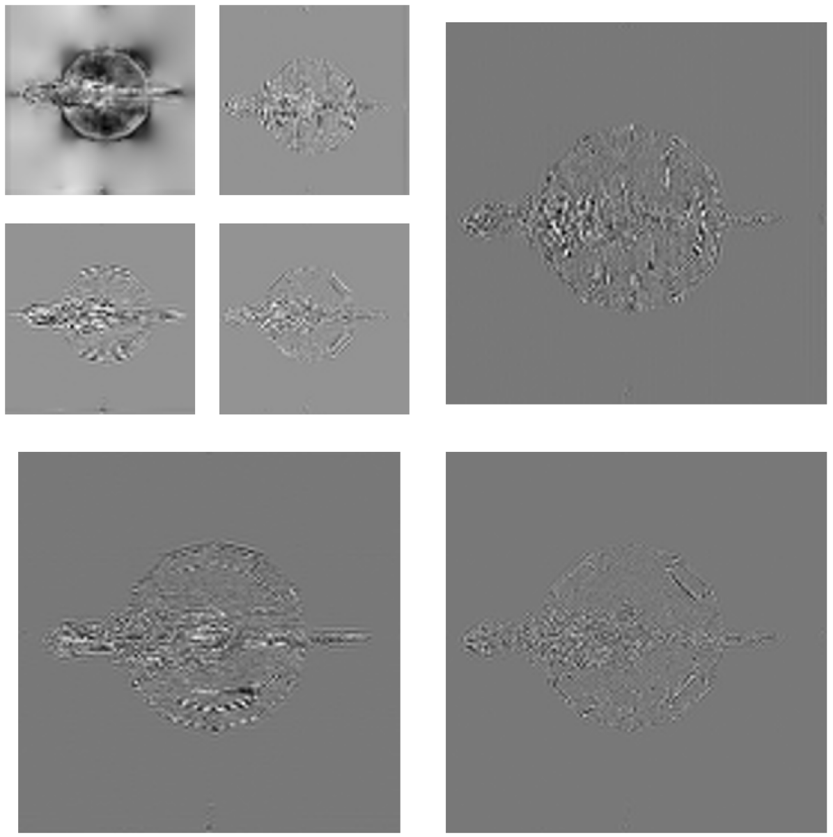
Figure 11: Visualising wavelet coefficient planes for the T-Rex D-NeRF scene representation. We use the 2-level wavelet decomposition that produces the $\mathbf{P}^{s}_{xy}$ feature plane to illustrate the coefficients at each level and for separate filter orientations. Small Images: The father wavelet plane (top left) has a resolution of 64$\times$64 and is surrounded by the vertical (top right), horizontal (bottom left) and diagonal (bottom right) mother wavelet coefficients. Large Images: The mother wavelet coefficients have a resolution of 128$\times$128 where the vertical (top right), horizontal (bottom left) and diagonal (bottom right) planes are shown.

Feature Planes.

The feature plane, $\mathbf{P}_{xy}^{0}$, is visualized in Figure 12 for the D-NeRF T-Rex scene.

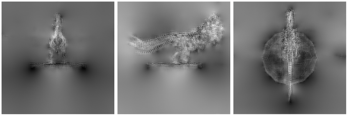
(a) Space-only Feature Planes

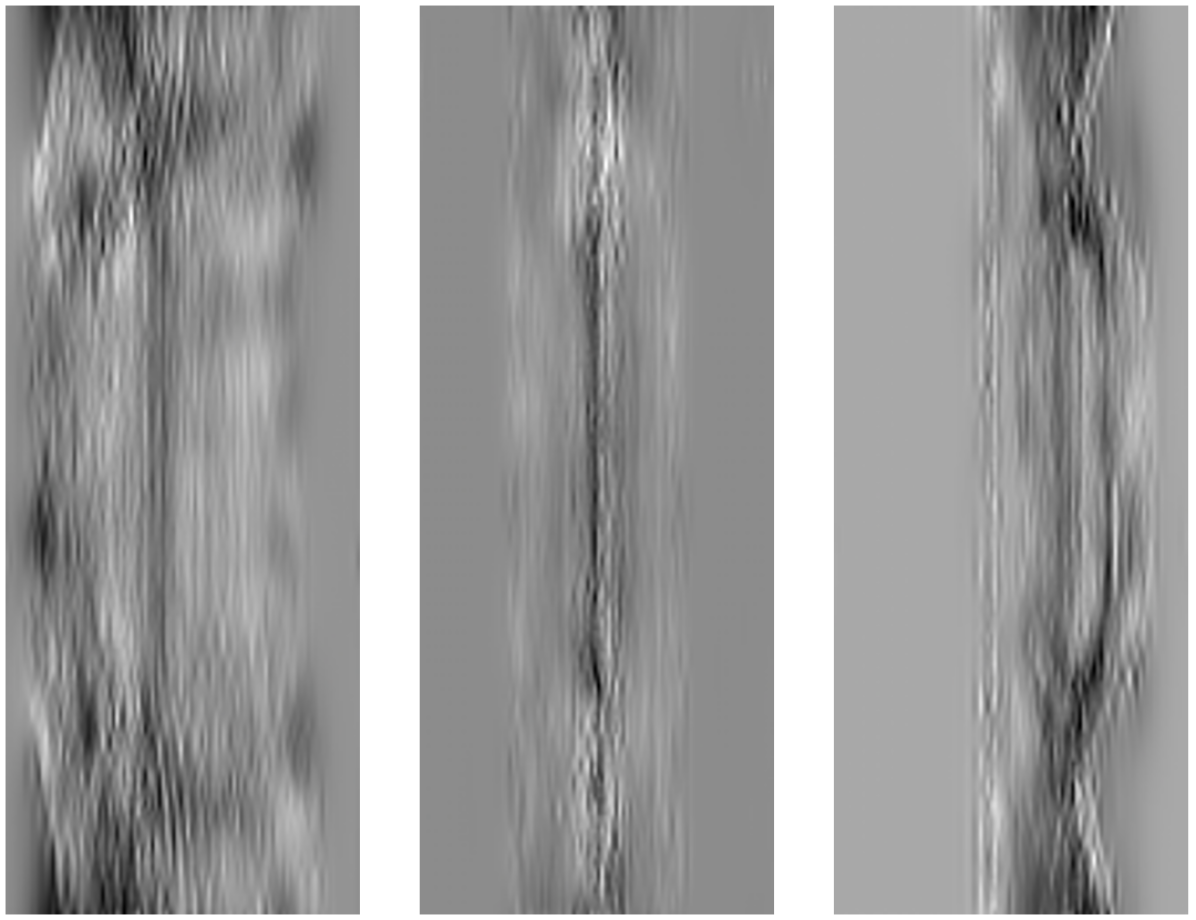
(b) Space-time Feature Planes

Figure 12: Visualising the space-only and space-time feature planes. Black to white pixels indicate negative to positive feature values, respectively. (a) Space-only feature planes are visualized. (b) Space-time features are visualized where the horizontal axis represents time.

C.3 Decomposing Static and Dynamic Components

In Figure 13, we exemplify the decomposition of our representation into static and dynamic components. To render a space-only scene (visualizing only static features), we force the condition $f_{c_{t}}(\mathbf{q})=1$ by zeroing the wavelet coefficients for all space-time planes. The space-only rendered frames are subtracted from the final render to visualize the effect of space-time features. Note that we do not use $f_{c\neq c_{t}}(\mathbf{q})=1$ to render space-time features directly as they can not be interpreted by the colour and density decoder. This adds to our interpretation of space-time features, whereby we treat them as linear transformations for the space-only features that can be interpreted as basis features. Interestingly, this behaviour is similar to dynamic NeRFs that use deformation fields to linearly transform the position of volumes in a static field. Though instead, the plane representation only modifies the density and color of volumes in time.

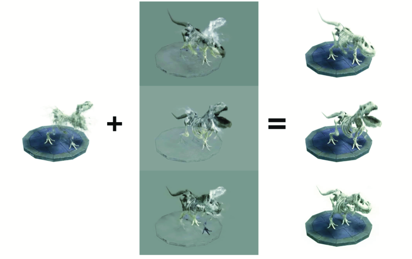
Figure 13: Visualising space and space-time separation on the T-Rex D-NeRF scene. Left: Space-only features are rendered. Right: All features are rendered. Center: All rendered features are subtracted from the space-only render, representing the effect of space-time features on the final render.

In Figure 14 we provide further visual comparison between the static decomposition of the HP and ZMM feature fusion schemes.

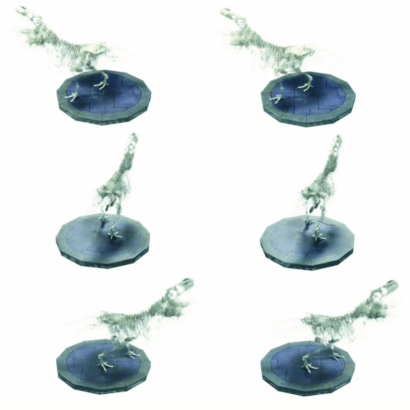
Figure 14: Visualising the static decomposition from HP (left) and ZMM (right) fused WavePlane models on the T-Rex D-NeRF scene. Less noise is present for the ZMM approach, e.g. around the tail and the lower jaw bones.

C.4 Ablation Study

N-level wavelet scaling coefficients.

To produce fair comparisons with the final model we used the results in Table 10 to tune a our model for a 2, 3 and 4 level of wavelet decomposition. We find that higher levels of decomposition results in slower training time and delayed convergence.

Scaling	PSNR $\uparrow$			SSIM $\uparrow$
$\mathbf{k}$	Whole	Front	Back
$N=2$ levels, 72 mins
$[1,1,1]$	31.30	20.63	76.01	0.977
$[1,0.8,0.4]$	31.31	20.64	75.78	0.978
$[1,0.4,0.2]$	31.34	20.67	78.05	0.978
$[1,0.8,0.2]$	31.33	20.66	76.75	0.978
$N=3$ levels, 84 mins
$[1,1,1,1]$	30.52	19.53	75.39	0.975
$[1,0.8,0.6,0.4]$	30.98	20.27	75.41	0.977
$[1,0.5,0.3,0.1]$	30.64	19.97	78.00	0.975
$[1,0.8,0.4,0.2]$	30.37	19.70	76.21	0.975
$N=4$ levels, 95 mins
$[1,1,1,1]$	30.03	19.37	62.34	0.973
$[1,0.5,0.4,0.2,0.1]$	30.65	19.98	75.08	0.975
$[1,0.8,0.6,0.4,0.2]$	30.22	19.56	69.29	0.974

Table 10: Level-dependant scaling coefficients, k, used for the comparing different levels of wavelet decomposition. Accomplished on the T-Rex D-NeRF scene. Training time is provided in minutes.

Varying weights for regularization.

The following outlines our process for tuning the weights for regularization - accomplished using the T-Rex and Hell Warrior D-NeRF scenes. We first optimized the TV weight in Table 11, where we selected a weight of 0.00001. After this we varied the SST weights. Table 12 outlines the results, showing that TV has a less of an impact on the performance. Finally, with an SST weight of 0.1 we varied the weight for ST regularization in Table 13.

Weight	PSNR $\uparrow$			SSIM $\uparrow$
	Whole	Front	Back
0.01	29.84	19.17	76.31	0.9696
0.001	30.70	20.03	78.89	0.9752
0.0001	30.89	20.22	77.52	0.9763
0.00001	30.97	20.31	74.36	0.9763

Table 11: Comparing different weights for ST regularisation on the T-Rex D-NeRF scene.

Weight	PSNR $\uparrow$			SSIM $\uparrow$
	Whole	Front	Back
0.1	31.06	20.39	78.58	0.9770
0.01	30.53	19.86	77.66	0.9756
0.001	29.45	18.83	77.18	0.9720
0.0001	28.88	18.21	76.50	0.9688

Table 12: Comparing different weights for SST regularisation on the T-Rex D-NeRF scene [20].

Weight	PSNR $\uparrow$			SSIM $\uparrow$
	Whole	Front	Back
0.01	21.55	11.77	51.46	0.9109
0.001	24.47	14.68	59.21	0.9415
0.0001	25.43	15.63	67.79	0.9504
0.00001	25.92	16.13	70.70	0.9545
0.000001	25.60	15.81	67.92	0.9520

Table 13: Comparing different weights for TV regularisation on the Hell Warrior D-NeRF scene.

Varying grid resolution.

For synthetic dynamic scenes our model performs best with a spatial resolution of $H=W=$256 for high-frequency and 128 for low-frequency scenes, as discussed in the paper. Results indicating this behavior are provided in Table 14. We notice longer training times with worse quantitative results when $P_{c}^{1}$ is significantly high in resolution, exemplified by the Lego and T-Rex scenes.

Resolution		PSNR $\uparrow$	SSIM $\uparrow$	Time $\downarrow$
$P^{0}_{c}$	$P^{1}_{c}$
T-Rex scene, D-NeRF [20]
128	64	30.88	0.9749	62
256	128	31.34	0.9782	72
512	256	30.75	0.9761	127
Lego, D-NeRF [20]
128	64	25.25	0.9380	60
256	128	25.19	0.9876	68
512	256	24.76	0.9377	113
Bouncing Balls, D-NeRF [20]
128	64	37.71	0.9876	70
256	128	36.66	0.9840	74
512	256	34.74	0.9802	110

Table 14: Varying the wavelet plane’s resolution for various D-NeRF scenes scenes. The resolution of the resulting features planes is shown, where the wavelet coefficients will have a maximum resolution half that of $P_{c}^{0}$.

Appendix D Paper Limitations

D.1 Quantitative Image Assessment Metrics

It is challenging to discern true dynamic performance from the variety of metrics that have been proposed, such as SSIM, D-SSIM [2], MS-SSIM [27] and LPIPS [33]. For synthetic RGBA data sets we also propose to separate foreground and background predictions during testing and validation. Considering that all these metrics evaluate stationary frames at different times, we are limited by our ability to evaluate temporal features such as smoothness and consistency. Additionally, the data sets we use do not support this type of evaluation. For instance, the D-NeRF data set is strictly provided as a set of ”teleporting” frames so could not be used for evaluating spatiotemproal smoothness using ground truth renders.

D.2 Hardware Failure Case

Our work began with 24 GB of GPU memory and 32 GB of RAM. This works for the D-NeRF and LLFF data sets. However, for the DyNeRF data set the amount of RAM required for IST weight generation is significant ($>$256GB). We were unable to attain during our research. Instead, we found that 98 GB of RAM was sufficient and low cost, despite limiting us to 8x down sampling for IST weight generation. Note, this has been previously discussed in the official K-Planes repository.

Appendix E Failed Designs

The final design was not the first solution we conceived. In this section we detail several technical designs that failed.

E.1 K-Planes Time Smoothness Regularizer

As our implementation initially branched off the K-Planes code, our earliest design utilized the TS regularizer proposed in [11] instead of the proposed SST regularizer. In Table 15 we compare the results from using TS regularization and SST regularization, showing that for WavePlanes the SST regularizer is a better fit.

$$\mathcal{L}_{TV}=\frac{1}{|C|n^{2}}\sum_{c,i,t}||\mathbf{P}^{i,t-1}_{c}-2\mathbf{P}^{i,t}_{c}+\mathbf{P}^{i,t+1}_{c}||^{2}_{2}$$ (11)

	PSNR $\uparrow$			SSIM $\uparrow$
	Front	Back	Whole
ZMM-SST	20.74	76.41	31.41	0.9781
ZMM-TS	18.70	75.29	29.37	0.9721

Table 15: Comparing SST and TS regularizers on the T-Rex D-NeRF scene [20].

E.2 Directly Smoothing Temporal Coefficients with Orientation

Each set of mother wavelet coefficients contains components for horizontal, diagonal and vertical filters which we define as $\Omega_{c,f}\in\mathbf{\Omega}_{c}$ where $f\in[horizontal,vertical,diagonal]$. This offers the opportunity to refactor the SST function (a 1-d Laplacian approximation of the planes second derivative) to regularize coefficient filters directly. This also allows us to prioritize smoothness for each filter direction, where the horizontal filter exists along the time-axis, the vertical filter along the spatial axis and the diagonal filter along $t=x=z=y$. Hence we use Equation 12 for each filter where $c=c_{t}$. To regularize the father wavelet coefficients, which do not contain directional filters, we apply the 1-D Laplacian approximation across the horizontal and vertical axis and add the result to $\mathcal{L}_{SST-horizontal}$ and $\mathcal{L}_{SST-vertical}$, respectively. For $f=diagonal$, we average the second order approximations along both axis’ of the father wavelet planes and add the result to $\mathcal{L}_{SST-diagonal}$. This ensures that all coefficients are regularized for a given orientation. The result of using these separately is compared with the proposed SST regularization in Table 16.

$$\mathcal{L}_{SST-f}=\frac{1}{|C|n^{2}}\sum_{c,i,t}||\mathbf{\Omega}^{i,t-1}_{c,f}-2\mathbf{\Omega}^{i,t}_{c,f}+\mathbf{\Omega}^{i,t+1}_{c,f}||^{2}_{2}$$ (12)

f	PSNR $\uparrow$
	Whole	Front
*	31.34	20.67
horizontal	29.23	18.55
diagonal	29.14	18.41
vertical	29.08	18.48

Table 16: Comparing directionally dependant smoothness regularizers on the wavelet coefficients for the T-Rex D-NeRF data set [20]. * indicates the final Wave Planes model which uses the proposed SST regularization.

References

- Attal et al. [2023] Benjamin Attal, Jia-Bin Huang, Christian Richardt, Michael Zollhoefer, Johannes Kopf, Matthew O’Toole, and Changil Kim. Hyperreel: High-fidelity 6-dof video with ray-conditioned sampling. In Proceedings of the IEEE/CVF Conference on Computer Vision and Pattern Recognition, pages 16610–16620, 2023.
- Baker et al. [2022] Allison H Baker, Alexander Pinard, and Dorit M Hammerling. Dssim: a structural similarity index for floating-point data. arXiv preprint arXiv:2202.02616, 2022.
- Barron et al. [2022] Jonathan T Barron, Ben Mildenhall, Dor Verbin, Pratul P Srinivasan, and Peter Hedman. Mip-nerf 360: Unbounded anti-aliased neural radiance fields. In Proceedings of the IEEE/CVF Conference on Computer Vision and Pattern Recognition, pages 5470–5479, 2022.
- Cao and Johnson [2023] Ang Cao and Justin Johnson. Hexplane: A fast representation for dynamic scenes. In Proceedings of the IEEE/CVF Conference on Computer Vision and Pattern Recognition, pages 130–141, 2023.
- Carroll and Chang [1970] J Douglas Carroll and Jih-Jie Chang. Analysis of individual differences in multidimensional scaling via an n-way generalization of “eckart-young” decomposition. Psychometrika, 35(3):283–319, 1970.
- Chen et al. [2022] Anpei Chen, Zexiang Xu, Andreas Geiger, Jingyi Yu, and Hao Su. Tensorf: Tensorial radiance fields. In European Conference on Computer Vision, pages 333–350. Springer, 2022.
- Cotter [2020] Fergal Cotter. Uses of complex wavelets in deep convolutional neural networks. PhD thesis, 2020.
- da Silva and Ghanbari [1996] Eduardo AB da Silva and Mohammed Ghanbari. On the performance of linear phase wavelet transforms in low bit-rate image coding. IEEE Transactions on Image Processing, 5(5):689–704, 1996.
- Fang et al. [2022] Jiemin Fang, Taoran Yi, Xinggang Wang, Lingxi Xie, Xiaopeng Zhang, Wenyu Liu, Matthias Nießner, and Qi Tian. Fast dynamic radiance fields with time-aware neural voxels. In SIGGRAPH Asia 2022 Conference Papers, pages 1–9, 2022.
- Fridovich-Keil et al. [2022] Sara Fridovich-Keil, Alex Yu, Matthew Tancik, Qinhong Chen, Benjamin Recht, and Angjoo Kanazawa. Plenoxels: Radiance fields without neural networks. In Proceedings of the IEEE/CVF Conference on Computer Vision and Pattern Recognition, pages 5501–5510, 2022.
- Fridovich-Keil et al. [2023] Sara Fridovich-Keil, Giacomo Meanti, Frederik Rahbæk Warburg, Benjamin Recht, and Angjoo Kanazawa. K-planes: Explicit radiance fields in space, time, and appearance. In Proceedings of the IEEE/CVF Conference on Computer Vision and Pattern Recognition, pages 12479–12488, 2023.
- Gan et al. [2023] Wanshui Gan, Hongbin Xu, Yi Huang, Shifeng Chen, and Naoto Yokoya. V4d: Voxel for 4d novel view synthesis. IEEE Transactions on Visualization and Computer Graphics, 2023.
- Harshman et al. [1970] Richard A Harshman et al. Foundations of the parafac procedure: Models and conditions for an” explanatory” multimodal factor analysis. 1970.
- Işık et al. [2023] Mustafa Işık, Martin Rünz, Markos Georgopoulos, Taras Khakhulin, Jonathan Starck, Lourdes Agapito, and Matthias Nießner. Humanrf: High-fidelity neural radiance fields for humans in motion. arXiv preprint arXiv:2305.06356, 2023.
- Li et al. [2022] Tianye Li, Mira Slavcheva, Michael Zollhoefer, Simon Green, Christoph Lassner, Changil Kim, Tanner Schmidt, Steven Lovegrove, Michael Goesele, Richard Newcombe, et al. Neural 3d video synthesis from multi-view video. In Proceedings of the IEEE/CVF Conference on Computer Vision and Pattern Recognition, pages 5521–5531, 2022.
- Li et al. [2023] Zhengqi Li, Qianqian Wang, Forrester Cole, Richard Tucker, and Noah Snavely. Dynibar: Neural dynamic image-based rendering. In Proceedings of the IEEE/CVF Conference on Computer Vision and Pattern Recognition, pages 4273–4284, 2023.
- Mildenhall et al. [2019] Ben Mildenhall, Pratul P. Srinivasan, Rodrigo Ortiz-Cayon, Nima Khademi Kalantari, Ravi Ramamoorthi, Ren Ng, and Abhishek Kar. Local light field fusion: Practical view synthesis with prescriptive sampling guidelines. ACM Transactions on Graphics (TOG), 2019.
- Mildenhall et al. [2021] Ben Mildenhall, Pratul P Srinivasan, Matthew Tancik, Jonathan T Barron, Ravi Ramamoorthi, and Ren Ng. Nerf: Representing scenes as neural radiance fields for view synthesis. Communications of the ACM, 65(1):99–106, 2021.
- Müller [2021] Thomas Müller. tiny-cuda-nn, 2021.
- Pumarola et al. [2021] Albert Pumarola, Enric Corona, Gerard Pons-Moll, and Francesc Moreno-Noguer. D-nerf: Neural radiance fields for dynamic scenes. In Proceedings of the IEEE/CVF Conference on Computer Vision and Pattern Recognition, pages 10318–10327, 2021.
- Rho et al. [2023] Daniel Rho, Byeonghyeon Lee, Seungtae Nam, Joo Chan Lee, Jong Hwan Ko, and Eunbyung Park. Masked wavelet representation for compact neural radiance fields. In Proceedings of the IEEE/CVF Conference on Computer Vision and Pattern Recognition, pages 20680–20690, 2023.
- Saragadam et al. [2023] Vishwanath Saragadam, Daniel LeJeune, Jasper Tan, Guha Balakrishnan, Ashok Veeraraghavan, and Richard G Baraniuk. Wire: Wavelet implicit neural representations. In Proceedings of the IEEE/CVF Conference on Computer Vision and Pattern Recognition, pages 18507–18516, 2023.
- Shao et al. [2023] Ruizhi Shao, Zerong Zheng, Hanzhang Tu, Boning Liu, Hongwen Zhang, and Yebin Liu. Tensor4d: Efficient neural 4d decomposition for high-fidelity dynamic reconstruction and rendering. In Proceedings of the IEEE/CVF Conference on Computer Vision and Pattern Recognition, pages 16632–16642, 2023.
- Shue et al. [2023] J Ryan Shue, Eric Ryan Chan, Ryan Po, Zachary Ankner, Jiajun Wu, and Gordon Wetzstein. 3d neural field generation using triplane diffusion. In Proceedings of the IEEE/CVF Conference on Computer Vision and Pattern Recognition, pages 20875–20886, 2023.
- Song et al. [2023] Liangchen Song, Anpei Chen, Zhong Li, Zhang Chen, Lele Chen, Junsong Yuan, Yi Xu, and Andreas Geiger. Nerfplayer: A streamable dynamic scene representation with decomposed neural radiance fields. IEEE Transactions on Visualization and Computer Graphics, 29(5):2732–2742, 2023.
- Wang et al. [2022] Liao Wang, Jiakai Zhang, Xinhang Liu, Fuqiang Zhao, Yanshun Zhang, Yingliang Zhang, Minye Wu, Jingyi Yu, and Lan Xu. Fourier plenoctrees for dynamic radiance field rendering in real-time. In Proceedings of the IEEE/CVF Conference on Computer Vision and Pattern Recognition, pages 13524–13534, 2022.
- Wang et al. [2003] Zhou Wang, Eero P Simoncelli, and Alan C Bovik. Multiscale structural similarity for image quality assessment. In The Thrity-Seventh Asilomar Conference on Signals, Systems & Computers, 2003, pages 1398–1402. Ieee, 2003.
- Wizadwongsa et al. [2021] Suttisak Wizadwongsa, Pakkapon Phongthawee, Jiraphon Yenphraphai, and Supasorn Suwajanakorn. Nex: Real-time view synthesis with neural basis expansion. In Proceedings of the IEEE/CVF Conference on Computer Vision and Pattern Recognition, pages 8534–8543, 2021.
- Xu et al. [2023] Muyu Xu, Fangneng Zhan, Jiahui Zhang, Yingchen Yu, Xiaoqin Zhang, Christian Theobalt, Ling Shao, and Shijian Lu. Wavenerf: Wavelet-based generalizable neural radiance fields. arXiv preprint arXiv:2308.04826, 2023.
- Yan et al. [2023] Zhiwen Yan, Chen Li, and Gim Hee Lee. Nerf-ds: Neural radiance fields for dynamic specular objects. In Proceedings of the IEEE/CVF Conference on Computer Vision and Pattern Recognition, pages 8285–8295, 2023.
- Yu et al. [2021] Alex Yu, Ruilong Li, Matthew Tancik, Hao Li, Ren Ng, and Angjoo Kanazawa. Plenoctrees for real-time rendering of neural radiance fields. In Proceedings of the IEEE/CVF International Conference on Computer Vision, pages 5752–5761, 2021.
- Zhang et al. [2020] Kai Zhang, Gernot Riegler, Noah Snavely, and Vladlen Koltun. Nerf++: Analyzing and improving neural radiance fields. arXiv preprint arXiv:2010.07492, 2020.
- Zhang et al. [2018] Richard Zhang, Phillip Isola, Alexei A Efros, Eli Shechtman, and Oliver Wang. The unreasonable effectiveness of deep features as a perceptual metric. In CVPR, 2018.