Cooperation Based Joint Active and Passive Sensing with Asynchronous Transceivers for Perceptive Mobile Networks

Abstract

Perceptive mobile network (PMN) is an emerging concept for next-generation wireless networks capable of conducting integrated sensing and communication (ISAC). A major challenge for realizing high performance sensing in PMNs is how to deal with spatially separated asynchronous transceivers. Asynchronicity results in timing offsets (TOs) and carrier frequency offsets (CFOs), which further cause ambiguity in ranging and velocity sensing. Most existing algorithms mitigate TOs and CFOs based on the line-of-sight (LOS) propagation path between sensing transceivers. However, LOS paths may not exist in realistic scenarios. In this paper, we propose a cooperation based joint active and passive sensing scheme for the non-LOS (NLOS) scenarios having asynchronous transceivers. This scheme relies on the cross-correlation cooperative sensing (CCCS) algorithm, which regards active sensing as a reference and mitigates TOs and CFOs by correlating active and passive sensing information. Another major challenge for realizing high performance sensing in PMNs is how to realize high accuracy angle-of-arrival (AoA) estimation with low complexity. Correspondingly, we propose a low complexity AoA algorithm based on cooperative sensing, which comprises coarse AoA estimation and fine AoA estimation. Analytical and numerical simulation results verify the performance advantages of the proposed CCCS algorithm and the low complexity AoA estimation algorithm.

I Introduction

I-A Background and Motivation

Perceptive mobile network (PMN) [[PMC_1], [AOA_9]] is an emerging concept for next-generation wireless networks that combine sensing and communication capabilities (ISAC) to serve as a ubiquitous environment sensing network while maintaining reliable mobile communication services [[PMC]]. In [[PMC_3]], Zhang et al. conducted an in-depth study on the capability of sensing the user equipment (UE) by the sensing base station (SBS) in PMN, and defined three types of sensing: downlink active sensing, downlink passive sensing, and uplink passive sensing. In a PMN, active sensing and passive sensing may co-exist [[PMC_3]]. For active sensing, the transmitter and receiver are co-located, which means that they can be conveniently synchronized at the clock level [[jwj_1], [jwj_2]]. However, for passive sensing, the transmitter and receiver are spatially separated and asynchronous, which results in timing offsets (TOs) and carrier frequency offsets (CFOs), thus leading to degradation of sensing accuracy with respect to ranging and velocity measurements.

To obtain high performance sensing in a PMN, joint active and passive sensing is advocated as a promising technique [[CS_4]], where cooperation between co-existing active sensing and passive sensing is exploited. A major challenge facing cooperation based joint active and passive sensing is how to achieve high performance passive sensing with spatially separated asynchronous transceivers. On the one hand, most existing passive or cooperative sensing algorithms assumed perfect synchronization between receivers and transmitters, and did not consider the influence of TOs and CFOs on the cooperative sensing performance [[CS_1], [CS_2], [CS_3]]. On the other hand, a few contributions resort to mitigate TOs and CFOs based on the line-of-sight (LOS) path between the sensing-oriented receiver and transmitter, but the LOS path may not exist in realistic scenarios [[Survey], [UL_sensing]]. For a PMN operating in the non-LOS (NLOS) environment, mitigating the TOs and CFOs in passive sensing remains an open problem that has to be solved.

Since the scale of antenna arrays deployed on SBS is limited, how to achieve high accuracy angle-of-arrival (AoA) estimation with limited-size antenna arrays is another challenge facing the cooperation based joint active and passive sensing. Most existing algorithms [[UL_sensing], [AOA_29], [AOA_30], [AOA_41]] use both time-domain and spatial-domain measurements to improve the accuracy of AoA estimation, but the computational complexity is excessively high. Therefore, how to realize high accuracy AoA estimation with low complexity in the context of PMN is also an important problem that needs to be solved.

I-B Related Work

There have been some related studies that are valuable for solving the above mentioned challenges confronting the cooperative sensing in PMN. The major state-of-the-art contributions are described as follows.

1) TO and CFO mitigation in the presence of asynchronicity:

In wireless communications, some efforts have been devoted to the asynchronicity problem in cognitive radio [[C_TO_CFO_1], [C_TO_CFO_2], [C_TO_CFO_3]]. However, these studies focused on the analysis of interference caused by asynchronicity, such as the inter-symbol interference (ISI) and inter-carrier interference (ICI) caused by TOs and CFOs [[C_TO_CFO_4], [C_TO_CFO_5]], without providing effective methods for parameter estimation.

In wireless sensing, TO and CFO can directly cause timing and Doppler estimation ambiguity and hence leading to degradation of sensing accuracy with respect to ranging and velocity measurements. Existing synchronization algorithms for sensing can be divided into three categories: GPS clock, and single-node-based and network-based solutions [[AJ_AS]].

• GPS clock synchronization is suitable for outdoor environments that can receive GPS signals. The synchronization accuracy of GPS-assisted synchronization is sufficient for communications, but not for target sensing. For example, for a typical GPS clock stability error of 20 ns, this translates into a ranging error of 6 m.

• Single-node-based synchronization can be implemented in a single receiver. The cross-antenna cross-correlation (CACC) method is a typical single-node-based synchronization algorithm, which is widely used in Wi-Fi sensing [[TO_CFO_25], [TO_CFO_26], [TO_CFO_27]]. However, the CACC method mitigate TOs and CFOs based on the assumption that there is a strong LOS path between the sensing receiver and transmitter, which may not be suitable in NLOS scenarios.

• Network-based synchronization exploits measurements from multiple cooperative nodes. One of the typical network-based synchronization method is the trilateration, which exploit known geometric relationships to remove TO and CFO [[AJ_AS_11]]. Other techniques deal with asynchrony by taking advantage of the statistical averaging effect of multiple measurements. However, the above methods have the problems of high complexity and difficult multi-target association, which could be concerns for real-time implementation.

2) AoA estimation for wireless sensing: Another major challenge for realizing high performance sensing in PMNs is how to accurately estimate the AoA of the target. AoA estimation algorithms based on the combination of multiple-domain information are proposed in [[AOA_29], [AOA_30], [UL_sensing]]. More specifically, Ni et al. [[UL_sensing]] attempte to equivalently extend the length of the spatial array response vector by integrating the time and frequency domain signals into the spatial domain, thereby obtaining higher accuracy in AoA estimation. In [[AOA_29]], Chuang et al. jointly combine spatial and temporal domain information to obtain high-accuracy AoA estimation. In [[AOA_30]], Ni et al. define a spatial path filter to separate signals sent over multiple propagation paths and obtain AoA through the CACC output. However, the above three algorithms that improve the accuracy of AoA estimation by expanding the length of the spatial array response vector lead to a substantial increase in the computational complexity.

I-C Main Contributions of Our Work

Against the above backdrop, we propose a cooperation based joint active and passive sensing scheme for improving the performance of SBS in a PMN that experiences the NLOS propagation, and our focus is on overcoming the asynchronicity problem in passive sensing and the low-complexity high-accuracy AoA estimation challenge with limited scale of antenna arrays. Our major contributions are summarized as follows.

1. Considering NLOS propagation, we provide a cooperation based joint active and passive sensing scheme that does not require clock-level synchronization between the spatially separated and asynchronous transceivers. Simulation results show that when the power of the active echo signal is close to that of the passive echo signal, the performance of cooperative sensing becomes appreciably superior to both the active sensing and passive sensing.

2. Considering the single target estimation scenario, we propose a cross-correlation cooperative sensing (CCCS) method that regards active sensing as a reference and mitigates TOs and CFOs existing in passive sensing by correlating active and passive sensing information. Compared with CACC proposed in [[UL_sensing]], CCCS is more widely applicable, because it does not require the existence of LOS propagation paths between transceivers.

3. Considering the multiple-target estimation scenario, we propose a multi-target alignment algorithm to handle the outputs of the CCCS method, so that the problem of inter-target correlation interference can be solved. Compared with the single target scenario, it is more challenging to estimate TOs and CFOs in the multi-target scenario by directly using CCCS, because in this situation the outputs of CCCS not only contain information on TOs and CFOs of the same target, but also contain information on the delay and Doppler spread correlation between different targets. This correlation may hamper the subsequent TOs and CFOs mitigation operations. The multi-target alignment algorithm includes two stages, i.e., the extraction stage and the matching stage. In the extraction stage, TOs and CFOs of the same target can be extracted with the aid of spatial information differences of different targets. Then TOs and CFOs of different targets are matched in the matching stage, as detailed in Section III-C2. Simulation results demonstrate that the multi-target alignment algorithm works well when the variance of CFOs is smaller than $\frac{1}{4}$ of the subcarrier spacing, which can be satisfied by ordinary frequency sources [[CFO_S_3], [CFO_S_4], [CFO_S_5]].

4. We develop a low-complexity high-accuracy AoA estimation algorithm based on cooperative sensing and fractional Fourier transform (FRFT). Although traditional FRFT can significantly improve the accuracy of AoA estimation, its way of expanding the number of Fourier transform points increases its computational complexity [[QHY]]. To reduce the complexity while ensuring high-accuracy AoA estimation, we propose an AoA estimation algorithm relying on iterations between coarse estimation and fine estimation. In the coarse estimation stage, we obtain a rough AoA result of targets by cooperative active and passive sensing. In the fine estimation stage, we further obtain a fine AoA of targets by the FRFT algorithm within the range of the rough AoA result. We analyze and simulate the accuracy and complexity of different AoA estimation algorithms, including the hybrid multiple signal classification (H-MUSIC) [[AOA_29]], hybrid estimation of signal parameters via rotational invariance techniques (H-ESPRIT) [[AOA_29]], joint time-space-frequency (TSF) domain MUSIC algorithm (TSF-MUSIC) [[UL_sensing]], and FRFT [[QHY]]. simulation results show that the AoA algorithm proposed in this paper can achieve relatively high-performance AoA estimation, close to FRFT, at a low complexity, much lower than FRFT.

The rest of this paper is organized as follows. In Section II we describe the system model of the cooperation based joint active and passive sensing. The cooperative sensing for delay and Doppler spread is introduced in Section III. In Section LABEL:sec:AOA we present the proposed low-complexity high-accuracy AoA estimation algorithm. Range, velocity and AoA estimation are analyzed and numerically evaluated in Section LABEL:sec:Simulation. Finally, Section LABEL:sec:Conclusion concludes the paper.

Notations: Vectors and matrices are denoted by boldface lowercase and uppercase letters; the transpose, complex conjugate, Hermitian, inverse, and pseudo-inverse of the matrix ${\bf{A}}$ are denoted by ${{\bf{A}}^{\rm T}}$, ${{\bf{A}}^{*}}$, ${{\bf{A}}^{\rm H}}$, ${{\bf{A}}^{-1}}$ and ${{\bf{A}}^{\dagger}}$, respectively; ${\rm{diag}}(\bf{x})$ denotes a diagonal matrix whose diagonal elements are the elements of $\bf x$; ${\mathcal{S}}(x_{i})$ denotes the set of $x_{i}$; $\otimes$ represents the Kronecker product; $\odot$ denotes the Hadamard product.

II System Model of Cooperative Sensing

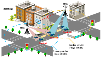
(a) SBS senses vehicle targets.

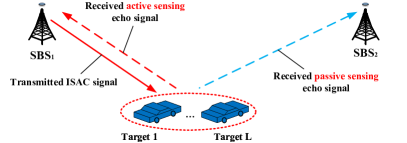
(b) Active and passive sensing

Figure 1: System model of cooperative sensing.

We consider the cooperation based joint active and passive sensing in a PMN. As Fig.  1 shows there is no LOS propagation path between $\rm{SBS}_{1}$ and $\rm{SBS}_{2}$ due to the occlusion of buildings. Each SBS with $N_{t}$ antennas, transmits ISAC signal to targets. These targets are not only sensing targets but also communication users. On the one hand, these targets obtain communication services by demodulating ISAC signals sent from SBS. On the other hand, SBS can receive the echo signal reflected by targets to realize the target sensing. These targets move along the road, across the sensing service range of $\rm{SBS}_{1}$ and $\rm{SBS}_{2}$. To provide continuous and high-performance sensing services for these targets, we propose a collaboration scheme between $\rm{SBS}_{1}$ and $\rm{SBS}_{2}$. It should be noted that, in this paper, we focuses on the use of ISAC technology to empower conventional communication base stations with sensing capabilities.

• In terms of signal design, we just reuses the OFDM communication signals of the existing base stations to achieve sensing without modification, and therefore, there is no significant interference to the communication performance.

• In terms of communication interaction, we just uses the echo signal reflected from the base station after the target for active and passive sensing, without destroying the original communication link, therefore, there is no obvious interference to the communication performance. Compared to the traditional communication base station, one of the biggest differences is that the ISAC base station needs to deploy two antenna arrays to simultaneously complete the ISAC signal transmission and echo signal reception. This can be done by increasing the cost of hardware to mitigate the degradation of communication performance.

Therefore, we think that the reduction in communication performance can be compensated by the use of appropriate technology and hardware cost inputs, and in this paper we do not focus on analyzing the specific performance of the communication link. There have been related studies on how to design ISAC waveforms to trade-off sensing and communication performance [[CD_OFDM]], which is not the focus of this paper and may be further investigated in future work.

II-A Cooperation between $\rm{SBS}_{1}$ and $\rm{SBS}_{2}$

As Fig. 1(a) shows, when targets in position A, in the sensing service range of $\rm{SBS}_{1}$, $\rm{SBS}_{1}$ can provide active sensing services for targets; when targets in position C, in the sensing service range of $\rm{SBS}_{2}$, $\rm{SBS}_{2}$ can provide active sensing services for targets. However, when targets in position B, in the sensing service overlap range of $\rm{SBS}_{1}$ and $\rm{SBS}_{2}$, the power of active sensing echo signal is weak, making it difficult for $\rm{SBS}_{1}$ and $\rm{SBS}_{2}$ to provide high-performance active sensing services for targets. We first use passive sensing to make up for the lack of performance of active sensing. However, the transceiver nodes of passive sensing are spatially separated asynchronously, resulting in TOs and CFOs, which further cause ambiguity in ranging and velocity sensing. To solve the above problem, we provide a cooperation based joint active and passive sensing scheme, including the following steps:

• Parameter setting: $\rm{SBS}_{1}$ and $\rm{SBS}_{2}$ adopt different signal parameters to distinguish the received active and passive sensing echo signals, as shown in Fig. 1(b). The techniques for separating echo signals of adjacent base stations are relatively mature, including time division (TD) scheme, frequency division (FD) scheme, code division (CD) scheme, etc. Although it is easier to distinguish between active and passive sensing signals in the TD scheme, active and passive sensing of the target cannot be simultaneously achieved by the SBS in this case [[TDD_1], [TDD_2], [TDD_4]]. By contrast, in the CD scheme, SBS can achieve active and passive sensing of the target at the same time, but it requires complex coding design and signal processing to distinguish between active and passive sensing signals [[TDD_3], [CD_OFDM]]. In this paper, under the condition of sufficient spectrum resources, we assume that adjacent SBSs adopt the FD scheme [[FDD_31]], which is widely adopted for adjacent base stations in the $4$-th generation (4G) and the $5$-th generation (5G) mobile communication systems [[3GPP_FD]].

• Initiation of cooperative sensing: When $\rm{SBS}_{1}$ receives the echo signal sent from $\rm{SBS}_{2}$, $\rm{SBS}_{1}$ will send a cooperative sensing request to $\rm{SBS}_{2}$. After receiving the reply of $\rm{SBS}_{2}$, the two SBSs will start cooperative sensing at the same time to generate a sensing beam pointing to the target area.

• Signal processing of cooperative sensing: When $\rm{SBS}_{1}$ receives the active and passive sensing echo signals, it will perform cooperative sensing based on CCCS, which will be described in detail in Section III.

II-B Received Signal Model of SBS

SBSs in a PMN can provide both sensing and communication services to UEs by transmitting ISAC signals. In the ISAC system, ISAC base stations not only need to improve sensing services, but also need to provide communication services for communication users. If the conventional sensing waveforms are used, it is difficult to guarantee the performance of the communication link. Therefore, the orthogonal frequency division multiplexing (OFDM) signal was used for joint sensing and communication [[OFDM_12]]. In terms of communication, OFDM signal is the waveform of the 4G and 5G mobile communication systems, hence it not only has advantages in mitigating multipath interference and exploiting frequency diversity, but also enjoys standard compatibility [[OFDM_2]]. In terms of sensing, OFDM signal has advantages in accuracy, resolution and flexibility [[OFDM_advantage]]. The number and the spacing of subcarriers can be adjusted flexibly to obtain the ambiguity function of “pushpin shape” [[OFDM_3]]. Therefore, OFDM signal is adopted as the sensing waveform of the SBS in this paper. Then, the received signal of ${\rm SBS}_{1}$ can be expressed as

$${y}(t) =\sum_{k=0}^{N_{t}-1}{y}_{1}(t)+{y}_{2}(t)+{z}(t),$$ (1)

where ${z}(t)$ is a complex additive white Gaussian noise (AWGN) vector with zero mean and variance of $\sigma^{2}$, ${y}_{1}(t)$ and ${y}_{2}(t)$ denote the echo signals from ${\rm SBS}_{1}$ and ${\rm SBS}_{2}$, respectively. The notation is defined as follows:

• $k$ is the index of antenna elements.

The active sensing echo signal from ${\rm SBS}_{1}$ and the passive sensing echo signal from ${\rm SBS}_{2}$ can be expressed as [[MIMO-OFDM], [MIMO-OFDM_GFF_1], [MIMO-OFDM_GFF_2], [MIMO-OFDM_JS_1], [MIMO-OFDM_JS_2], [MIMO-OFDM_WXD_1]]

$${{y}_{1}(t)} =\sum_{m=0}^{M-1}\sum_{n=0}^{N-1}\overbrace{d_{1,\textrm{Tx}}(k,m,n)\times\sum_{l=0}^{L-1}\alpha_{1,l}e^{j{\Omega}_{l}k}e^{-j2\pi n\Delta f{\tau_{1,l}}}\times e^{j2\pi mTf_{D,1,l}}}^{d_{1,\textrm{Rx}}(k,m,n)}$$ (2)

$$\cdot e^{-j2\pi(f_{\textrm{c1}}+n\Delta f)t}\cdot{\rm rect}\left(\frac{t-mT-\tau_{1,l}}{T}\right),$$ (3)

$${{y}_{2}(t)} =\sum_{m=0}^{M-1}\sum_{n=0}^{N-1}\overbrace{d_{2,\textrm{Tx}}(k,m,n)\times\sum_{l=0}^{L-1}\alpha_{2,l}e^{j{\Omega}_{l}k}e^{-j2\pi n\Delta f(\tau_{2,l}+\delta_{\tau}(m))}\times e^{j2\pi mT(f_{D,2,l}+\delta_{f}(m))}}^{d_{2,\textrm{Rx}}(k,m,n)}$$ (4)

$$\cdot e^{-j2\pi(f_{\textrm{c2}}+n\Delta f)t}\cdot{\rm rect}\left(\frac{t-mT-\tau_{2,l}-{\delta_{\tau}(m)}}{T}\right),$$ (5)

where ${\rm rect}\{\cdot\}$ denotes a rectangular window function. The rest of the notations and terms can be defined as follows:

• ${\bf a}({\Omega}_{l})$ is the receive steering vector of the $l$-th target with ${\Omega}_{l}=\frac{2\pi d}{\lambda}{\rm{cos}}(\theta_{l})$,

• $d$ is the distance between adjacent antenna elements,

• ${\lambda}$ is the wavelength of the signal,

• $\theta_{l}$ is the direction of the $l$-th target,

• $M$ and $N$ represent the number of OFDM symbols and the number of subcarriers,

• $m$ and $n$ are the indices of the OFDM symbols and the subcarriers, respectively,

• $f_{\textrm{c1}}$ and $f_{\textrm{c2}}$ are the carrier frequency of the active sensing and passive sensing echo signal,

• $L$ is the number of targets,

• $T$ is the length of an OFDM symbol,

• $\Delta f$ is the carrier spacing of OFDM signals.

• $d_{1,\textrm{Rx}}(k,m,n)$ and $d_{2,\textrm{Rx}}(k,m,n)$ are the received modulation symbols of the $k$-th antenna on $\rm{SBS}_{1}$ and $\rm{SBS}_{2}$,

• $d_{1,\textrm{Tx}}(k,m,n)$ and $d_{2,\textrm{Tx}}(k,m,n)$ are the transmitted modulation symbols of the $k$-th antenna on $\rm{SBS}_{1}$ and $\rm{SBS}_{2}$,

• $\tau_{1,l}$ and $f_{D,1,l}$ are the delay and Doppler spread between the $l$-th target and $\rm{SBS}_{1}$,

• $\tau_{2,l}$ and $f_{D,2,l}$ are the delay and Doppler spread between the $l$-th target and $\rm{SBS}_{2}$,

• $\alpha_{1,l}$ and $\alpha_{2,l}$ are the channel fading magnitudes of the $l$-th target in active and passive sensing,

• $\delta_{\tau}(m)$ and $\delta_{f}(m)$ denote the unknown time-varying TO and CFO [[TO_CFO_1], [TO_CFO_26]].

III Delay and Doppler Spread Estimation Based on CCCS

According to Section II-B, the delay and Doppler spread are mixed with TOs and CFOs, respectively. In this section, we propose the CCCS based algorithm to mitigate TOs and CFOs for achieving high-accuracy target delay and Doppler spread estimation. The CCCS based algorithm for delay and Doppler spread estimation consists of the following steps.

III-A Extracting Sensing Information

Based on (1), (4) and (5), the transmitted and received modulation symbols of the $k$-th antenna array from $\rm{SBS}_{1}$ and $\rm{SBS}_{2}$ can be rewritten as matrices, ${\bf D}_{1,\textrm{Tx}}(k)$, ${\bf D}_{2,\textrm{Tx}}(k)$, ${\bf D}_{1,\textrm{Rx}}(k)$, ${\bf D}_{2,\textrm{Rx}}(k)$, in which each column represents a OFDM symbol and each row represents a subcarrier. The sensing information can be extracted from the received modulation symbols by a point-wise complex division. Since the transmitted signal is modulated by quadrature phase shift keying (QPSK) in this paper, the amplitude of the transmitted OFDM modulation symbol is a non-zero constant, the noise enhancement caused by point-wise complex division is not serious [[CD_OFDM]]. Without loss of generality, we take the example of extracting sensing information from ${\bf D}_{1,\textrm{Rx}}(k)$ [[OFDM], [WK-OFDM]]

$$\begin{aligned} {\bf D}_{\textrm{div}}(k)&=\frac{{\bf D}_{1,\textrm{Rx}}(k)}{{\bf D}_{1,\textrm{Tx}}(k)}={\bf k}_{1,{R}}(k)\otimes{\bf k}_{1,{D}}(k)\end{aligned},$$ (6)

where $\otimes$ is the Kronecker product operator and

$$\begin{aligned} {\bf k}_{1,{R}}(k)&=\sum_{l=0}^{L-1}\alpha_{1,l}e^{j{\Omega}_{l}k}{\begin{bmatrix}1,&\cdots,&e^{-j2\pi n\Delta f\tau_{1,l}},&\cdots,&e^{-j2\pi(N-1)\Delta f\tau_{1,l}}\end{bmatrix}}^{\textrm{T}}\end{aligned},$$ (7)

$$\begin{aligned} {\bf k}_{1,{D}}(k)&=\sum_{l=0}^{L-1}\alpha_{1,l}e^{j{\Omega}_{l}k}{\begin{bmatrix}1,&\cdots,&e^{j2\pi mTf_{D,1,l}},&\cdots,&e^{j2\pi(M-1)Tf_{D,1,l}}\end{bmatrix}}^{\textrm{T}}\end{aligned},$$ (8)

are the range and Doppler spread steer vectors of active sensing.

Similarly, ${\bf k}_{2,{R}}(k)$ and ${\bf k}_{2,{D}}(k)$ can be obtained by extracting sensing information from from ${\bf D}_{2,\textrm{Rx}}$

$$\begin{aligned} {\bf k}_{2,{R}}(k)&=\sum_{l=0}^{L-1}\alpha_{2,l}e^{j{\Omega}_{l}k}{\begin{bmatrix}1,&\cdots,&e^{-j2\pi n\Delta f(\tau_{2,l}+\delta_{\tau}(m))},&\cdots,&e^{-j2\pi(N-1)\Delta f(\tau_{2,l}+\delta_{\tau}(m))}\end{bmatrix}}^{\textrm{T}}\end{aligned},$$ (9)

$$\begin{aligned} {\bf k}_{2,{D}}(k)&=\sum_{l=0}^{L-1}\alpha_{2,l}e^{j{\Omega}_{l}k}{\begin{bmatrix}1,&\cdots,&e^{j2\pi mT(f_{D,2,l}+\delta_{f}(m))},&\cdots,&e^{j2\pi(M-1)T(f_{D,2,l}+\delta_{f}(m))}\end{bmatrix}}^{\textrm{T}}\end{aligned}.$$ (10)

III-B Deviation Analysis of Cooperative Active and Passive Sensing

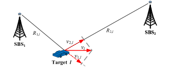
Figure 2: Active and passive sensing for the $l$-th target.

Due to the different location information of $\rm{SBS}_{1}$ and $\rm{SBS}_{2}$, there are deviations in the delay and Doppler spread estimation of active and passive sensing for the same target, which needs to be mitigated in order to achieve high accurate cooperative sensing. Without loss of generality, we consider the active and passive sensing for the $l$-th target. As Fig. 2 shows, the distance from the $l$-th target to $\rm{SBS}_{1}$ and $\rm{SBS}_{2}$ is $R_{1,l}$ and $R_{2,l}$, the velocity of target in the direction of $\rm{SBS}_{1}$ and $\rm{SBS}_{2}$ is $v_{1,l}$ and $v_{2,l}$. The delay, $\tau_{1,l}$ and $\tau_{2,l}$ can be expressed as

$$\begin{aligned} \tau_{1,l}=\frac{2R_{1,l}}{c},\quad\tau_{2,l}=\frac{R_{1,l}+R_{2,l}}{c}\end{aligned},$$ (11)

where $c$ is the speed of signal, $R_{1,l}$ and $R_{2,l}$ are the range from the $l$-th target to $\rm{SBS}_{1}$ and $\rm{SBS}_{2}$, respectively. Then the deviation of active and passive sensing in terms of delay estimation is

$$\begin{aligned} \Delta\tau_{l}&=\tau_{2,l}-\tau_{1,l}=\frac{R_{2,l}-R_{1,l}}{c}\end{aligned}.$$ (12)

Similarly, the Doppler spread, $f_{{D},1,l}$ and $f_{{D},1,l}$ can be expressed as

$$\begin{aligned} f_{{D},1,l}=\frac{2v_{1,l}f_{\textrm{c1}}}{c},\quad f_{{D},2,l}=\frac{(v_{1,l}-v_{2,l})f_{\textrm{c2}}}{c}\end{aligned},$$ (13)

and the deviation of active and passive sensing in terms of Doppler spread estimation $\Delta f_{{D},l}$ can be derived as

$$\begin{aligned} \Delta f_{{D},l}&=f_{{D},2,l}-f_{{D},1,l}=\frac{v_{1,l}(f_{\textrm{c2}}-f_{\textrm{c1}})}{c}-\frac{(v_{1,l}+v_{2,l})f_{\textrm{c2}}}{c}\end{aligned},$$ (14)

where $v_{1,l}$ and $v_{2,l}$ are the velocity of the $l$-th target in the direction from $\rm{SBS}_{1}$ to the $l$-th target and from the $l$-th target to $\rm{SBS}_{2}$.

III-C CCCS for Mitigating TOs and CFOs

To obtain better sensing performance by fusing the sensing signals of active and passive sensing, it is necessary to mitigate TOs and delay deviation of passive sensing in range measurement, and to mitigate the CFOs and Doppler spread deviation of passive sensing in velocity measurement. The CCCS based algorithm is proposed to mitigate TOs plus delay deviation and CFOs plus Doppler spread deviation by correlating active and passive sensing information. Specifically, the CCCS based algorithm regards the active sensing echo signal as a reference signal, and mitigates TOs and CFOs in the passive sensing echo signal by correlating the active and passive echo signals, which is named the CCCS algorithm.

III-C1 Single target

For single target, i.e., $L=1$, we perform the same CCCS algorithm for the received signal on each antenna. Without loss of generality, taking the $0$-th antenna as an example, i.e., $k=0$, then $e^{j\Omega_{l}k}=1$. Then, the active and passive sensing information normalized vectors can be re-expressed as

$$\begin{aligned} {\bf k}_{1,{R}}&={\begin{bmatrix}1,&\cdots,&e^{-j2\pi(N-1)\Delta f\tau_{1}}\end{bmatrix}}^{\textrm{T}},\qquad\qquad{\bf k}_{1,{D}}={\begin{bmatrix}1,&\cdots&e^{j2\pi(M-1)Tf_{{D},1}}\end{bmatrix}}^{\textrm{T}},\\ {\bf k}_{2,{R}}&={\begin{bmatrix}1,&\cdots,&e^{-j2\pi(N-1)\Delta f(\tau_{2}+\delta_{\tau}(m))}\end{bmatrix}}^{\textrm{T}},\quad{\bf k}_{2,{D}}={\begin{bmatrix}1,&\cdots,&e^{j2\pi(M-1)T(f_{{D},2}+\delta_{f}(m))}\end{bmatrix}}^{\textrm{T}}\end{aligned}.$$ (15)

Deviations of delay and Doppler spread between active and passive sensing for the same target can be re-expressed as $\Delta\tau$ and $\Delta f_{{D}}$, respectively. For mitigating $\Delta\tau+\delta_{\tau}(m)$, the CCCS algorithm between ${\bf k}_{1,{R}}$ and ${\bf k}_{2,{R}}$ generates

$$\begin{aligned} {\bf\rho}_{{R}}&={\rm{diag}}({\bf k}_{2,{R}}^{\textrm{H}})\cdot{\bf k}_{1,{R}}&={\begin{bmatrix}1,&\cdots,&e^{j2\pi n\Delta f(\Delta\tau+\delta_{\tau}(m))},&\cdots,&e^{j2\pi(N-1)\Delta f(\Delta\tau+\delta_{\tau}(m))}\end{bmatrix}}^{\textrm{T}}\end{aligned}.$$ (16)

For mitigating $\Delta f_{{D}}+\delta_{f}(m)$, the CCCS algorithm between ${\bf k}_{1,{D}}$ and ${\bf k}_{2,{D}}$ generates

$$\begin{aligned} {\bf\rho}_{{D}}&={\rm{diag}}({\bf k}_{2,{D}}^{\textrm{H}})\cdot{\bf k}_{1,{D}}&={\begin{bmatrix}1,&\cdots,&e^{-j2\pi mT(\Delta f_{{D}}+\delta_{f}(m))},&\cdots,&e^{-j2\pi(M-1)T(\Delta f_{{D}}+\delta_{f}(m))}\end{bmatrix}}^{\textrm{T}}\end{aligned}.$$ (17)

where $\Delta\tau+\delta_{\tau}(m)$ translates into a linear phase shift between the modulation symbols along the carrier frequency axis, $\Delta f_{{D}}+\delta_{f}(m)$ translates into a linear phase shift between the modulation symbols along the OFDM symbol axis. Thus, $\Delta\tau+\delta_{\tau}(m)$ and $\Delta f_{{D}}+\delta_{f}(m)$ can be estimated by the discrete Fourier transform (DFT) algorithm [[OFDM]].

III-C2 Multiple targets

Compared with the single target scenario, it is more difficult to obtain TOs and CFOs for multiple targets by CCCS algorithm because of the problem of inter-target correlation interference. To overcome this challenge, we propose a multi-target alignment algorithm to handle the outputs of the CCCS method for multiple targets.

According to (7), (8), (9) and (10), we can obtain the active sensing information vector, ${\bf k}_{1,{R}}(k)$, ${\bf k}_{2,{R}}(k)$ and passive sensing information vector, ${\bf k}_{1,{D}}(k)$, ${\bf k}_{2,{D}}(k)$. For mitigating $\Delta\tau_{l}+\delta_{\tau}(m)$, the CCCS algorithm between ${\bf k}_{1,{R}}(k)$ and ${\bf k}_{2,{R}}(k)$ generates

$$\begin{aligned} {\bf\rho}_{{R}}(k)&={\rm{diag}}({\bf k}_{2,{R}}^{\textrm{H}}(k))\cdot{\bf k}_{1,{R}}(k)&={\begin{bmatrix}\beta_{R}(0,k),&\cdots,&\beta_{R}(n,k),&\cdots,&\beta_{R}(N-1,k)\end{bmatrix}}^{\textrm{T}}\end{aligned},$$ (18)

where

$$\begin{aligned} \beta_{R}(n,k)&=\sum_{l_{1}=0}^{L-1}\sum_{l_{2}=0}^{L-1}\alpha_{1,l_{1}}\alpha_{2,l_{2}}\cdot e^{j(\Omega_{l_{1}}-\Omega_{l_{2}})k}e^{j2\pi n\Delta f(\tau_{2,l_{2}}-\tau_{1,l_{1}}+\delta_{\tau}(m))}\end{aligned},$$ (19)

which can be split into two parts, $D_{R}(n,k)$ and $I_{R}(n,k)$.

$$\begin{aligned} D_{R}(n,k)&=\sum_{l=0}^{L-1}\alpha_{1,l}\alpha_{2,l}e^{j(\Omega_{l}-\Omega_{l})k}e^{j2\pi n\Delta f(\tau_{2,l}-\tau_{1,l}+\delta_{\tau}(m))}\\ &=\sum_{l=0}^{L-1}\alpha_{1,l}\alpha_{2,l}e^{j2\pi n\Delta f(\Delta{\tau}_{l}+\delta_{\tau}(m))}\end{aligned},$$ (20)

$$\begin{aligned} I_{R}(n,k)&=\sum_{l_{1}=0}^{L-1}\sum_{l_{2}=0,l_{2}\neq l_{1}}^{L-1}\alpha_{1,l_{1}}\alpha_{2,l_{2}}e^{j(\Omega_{l_{1}}-\Omega_{l_{2}})k}\cdot e^{j2\pi n\Delta f(\tau_{2,l_{2}}-\tau_{1,l_{1}}+\delta_{\tau}(m))}\end{aligned}.$$ (21)

According to (19), (20) and (21), the CCCS outputs for multiple targets not only contains information on TOs and CFOs of the same target, $D_{R}(n,k)$, but also time delay and Doppler spread correlation information between different targets, $I_{R}(n,k)$, which will interfere with the subsequent TOs and CFOs mitigation operations. To overcome this problem, we propose a CCCS based algorithm for multiple targets, including two stages, i.e., the extraction stage and the matching stage. In the extraction stage, we conduct $\delta_{\tau}(m)+\Delta\tau_{l}$ and $\Delta\tau+\Delta f_{{D},l}$ extraction without differentiating between different targets, and we match them for different targets in the matching stage.

For above CCCS outputs, we have the proposition that $D_{R}(n,k)$ is invariant with $k$ and $I_{R}(n,k)$ is variant with $k$. Based on the above proposition, we can firstly obtain the set of phase information in $\beta_{R}(n,k)$ by the DFT algorithm [[OFDM]]. Then, the phase set of $D_{R}(n,k)$ can be extracted by continuously adjusting $k$, observing whether the DFT output of corresponding phases change, as shown in Algorithm III-C2.

  Algorithm 1 $\Delta{\tau}_{l}+\delta_{\tau}(m)$ extraction method

 

0:  

  ⋅TheCCCSoutputbasedon(18),ρ