Efficient LDPC Decoding using Physical Computation

Abstract

Due to 5G deployment, there is significant interest in LDPC decoding. While much research is devoted on efficient hardwiring of algorithms based on Belief Propagation (BP), it has been shown that LDPC decoding can be formulated as a combinatorial optimization problem, which could benefit from significant acceleration of physical computation mechanisms such as Ising machines. This approach has so far resulted in poor performance. This paper shows that the reason is not fundamental but suboptimal hardware and formulation. A co-designed Ising machine-based system can improve speed by 3 orders of magnitude. As a result, a physical computation approach can outperform hardwiring state-of-the-art algorithms. In this paper, we show such an augmented Ising machine that is 4.4$\times$ more energy efficient than the state of the art in the literature.

I Introduction

Error-correcting codes (ECCs) are essential in detecting and correcting errors in modern communication and storage infrastructures. The central idea of any ECC is to encode redundant information into the message sent. The redundancy allows the receiver to deal with a limited number of errors induced by the communication channel or storage media. There have been many ECCs introduced in literature, such as Hamming codes [1], convolutional codes [2], polar codes [3], turbo codes [4], etc. However, among them, low density parity check (LDPC) codes [5] have become more popular due to their ability to achieve the Shannon limit [6]. Recently they have been introduced in the 5G-NR standard along with Polar codes [7].

Decoding LDPC is at the moment computationally intensive. Perhaps the most popular approach to LDPC decoding is a Belief Propagation (BP) type algorithm. More specifically, more than 200 ASIC designs have been discussed in literature [8, 9] all using some variant of the Min-Sum algorithm [10], where an approximation is applied to the canonical BP algorithm to reduce computational intensity. An alternative approach to LDPC decoding is to treat it as a combinatorial optimization problem (COP). Algorithmically, Min-Sum variants are far more efficient than a typical COP solver when targeting real-world LDPC decoding. However, the latter can benefit from orders-of-magnitude acceleration from emerging hardware Ising machines [11, 12, 13]. Indeed, one such design using D-Wave’s quantum annealer was found to outperform an FPGA-based implementation of a variant of BP [14].

Nevertheless, LDPC decoding using Ising machines is not yet competitive with the state-of-the-art ASIC designs hard-wiring Min-Sum algorithm. Depending on the details of the custom hardware, these ASICs can expect a decoder throughput of roughly 0.13 - 271Gbps, with a power consumption of 5mW - 12W. Using D-Wave hardware to solve an LDPC decoding problem today can only achieve 21 Mb/s throughput, not to mention the kilo-watt power consumption. Of course, part of that is specific to D-Wave hardware. But there are intrinsic reasons as well. In this paper, we change this picture and show an efficient LDPC decoder based on physical computation with the following contributions:

1. Fundamental analysis: we show an important factor prohibiting out-performance is in current problem formulation when mapping to an Ising machine.

2. Co-designed architecture: We address this problem by proposing a novel, co-designed Ising machine architecture that allows better expressivity of the target problem.

3. Evaluation: Using detailed simulation, we show decoding throughput of 81 Gbits/sec and a power consumption of 158.24mW, representing at least 4 times reduction in energy compared to state-of-the-art decoder ASICs for 5G standards.

II Background and Related Work

We first discuss the communication model assumed. We then discuss LDPC codes and the Ising model.

II-A Communication model

In a general communication system, a message $M$ is first encoded using an encoder into a code word $C$. This code word is modulated using a modulator into the signal to be sent. While being transmitted, the signal gets affected by noise present in the channel. The received signal is then demodulated and decoded to recover the original message $M$, hopefully error free.

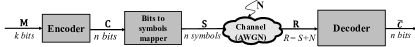
Figure 1: Schematic diagram of communication system.

In this paper, we assumed a discrete communication system (Fig. 1), where a binary message $M$ with $k$-bit is encoded into an $n$-bit code word $C$ using a ($k$, $n$) LDPC code. This code word is converted into an $n$-bit vector ($S_{i}=1-2C_{i}$) of symbols representing a binary phase shift keying (BPSK) constellation. This $n$-bit vector of symbols is transmitted over a channel with additive white Gaussian noise (AWGN). At the receiver end, we would receive a signal where $R_{i}=S_{i}+N(1/SNR)$, $N$ represents the channel’s noise.

II-B Low Density Parity Check Codes

LDPC codes are a class of linear block codes. The parity bits (redundant information) are obtained using bitwise XOR operation on a selected number of message bits. These codes are specified by a generator matrix $G_{k\times n}$ or a parity check matrix $H_{m\times n}$, each of which can be obtained from the other using the following relation $H\oplus G^{\top}=0$. Here $m$ is the number of parity bits, $n$ is the number of bits of the code word, and $k$ is the number of bits in the message ($k=n-m$). The ratio of the length of the message ($k$) to the size of the code word ($n$) is called the rate: $r=k/n$. For example, the 5G standard uses 1/3 and 1/5 rate codes. The generator matrix is used for encoding a message ($M$) into a code word ($C$) using the following equation $C=G^{\top}\oplus M$. At the receiver side the decoded message is obtained from both the received message ($R$) and the parity check matrix. The name “low density” comes from the sparse structure of the parity check matrix.

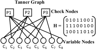
Figure 2: Tanner graph with corresponding parity check matrix $H$.

LDPC codes can be represented graphically using Tanner graphs. These graphs are bipartite, meaning that the graph nodes are separated into two distinctive sets, and edges only connect nodes of two different types. The two types of nodes in a Tanner graph are variable and check nodes. Fig. 2 is an example of a Tanner graph that is constructed using parity check matrix $H$ shown above. It consists of $m$ check nodes (the number of parity bits) and $n$ variable nodes (the number of bits in an encoded message). Check node $P_{i}$ is connected to variable node $C_{j}$ if the element $h_{ij}$ of $H$ is a 1. These graphical structures are handy for analysis and decoding purposes.

II-C Ising Model

The Ising model is used to describe the energy of a system of coupled spins. The spins have one degree of freedom and take one of two values ($+1$, $-1$). The energy of the system is a function of pair-wise coupling of the spins ($J_{ij}$) and the interaction ($h_{i}$) of some external field ($\mu$) with each spin. The resulting energy is as follows:

$$E=-\sum_{\mathclap{(i<j)}}J_{ij}\sigma_{i}\sigma_{j}-\mu\sum_{\mathclap{i}}h_{i}\sigma_{i}$$ (1)

A physical system with its energy defined by the formula naturally tends towards low-energy states. It is as if nature tries to solve an optimization problem with Eq. 1 as the objective function, which is not a trivial task. Indeed, the cardinality of the state space grows exponentially with the number of spins, and the optimization problem is NP-complete: it is easily convertible to and from a generalized max-cut problem, which is part of the original list of NP-complete problems [15].

Thus if a physical system of spins somehow offers programmable coupling parameters ($J_{ij}$ and $\mu h_{i}$ in Eq. 1), they can be used as a special purpose computer to solve optimization problems that can be expressed in the form of an Ising formula (Eq. 1). In fact, all problems in the Karp NP-complete set have their Ising formula derived [16]. Also, if a problem already has a QUBO (quadratic unconstrained binary optimization) formulation, mapping to Ising formula is as easy as substituting bits for spins, e.g., $\sigma_{i}=2b_{i}-1$.

Because of the broad class of problems that can map to the Ising formula, building nature-based computing systems that solve these problems has attracted significant attention [17, 18, 19, 20, 21, 22, 23, 24, 25].

III Co-designed Ising Machine Architecture

III-A Fundamentals of QUBO formulation of LDPC decoding

The goal of LDPC decoding is to reproduce the original message $M$ with low bit error rates. This is modeled as a combinatorial optimization problem with two objectives:

1. The decoded output $\tilde{C}$ is a code word (satisfies parity check).

2. It should be close to the received message $R$.

If we use the BPSK modulation scheme, the objective function can be represented by Eq. 2 where $\alpha$ adjusts the relative emphasis of the two objectives above.

$$\begin{split}F=\sum_{i=0}^{n-1}(R_{i}-(1-2\tilde{C_{i}}))^{2}+\alpha(H\oplus\tilde{C})\end{split}$$ (2)

III-A1 Conversion to QUBO formulation

Fundamentally, because of the presence of the XOR operation, Eq. 2 is not a quadratic formula (e.g., QUBO). Therefore it can not be directly mapped to an Ising machine. There are multiple ways of converting the formulation into a quadratic form, but here we only discuss one, which uses minimum auxiliary spins [26]. The general idea is straightforward: Satisfying parity check means that $H\oplus\tilde{C}$ is an all-zero vector. This in turns means that the inner product of each row of $H$ with $\tilde{C}$ is an even number. This can be represented as $H_{j}\cdot\tilde{C}=2L_{j}$, where $H_{j}$ is the $j$-th row of the parity check matrix ($H$), and $L_{j}$ is any integer. This condition can be represented using the following objective function:

$$F_{s}=\sum_{j=0}^{m-1}(\sum_{i=0}^{n-1}H_{j,i}\tilde{C}_{i}-2L_{j})^{2}.$$ (3)

Since the integer $L_{j}$ is a free variable, it needs to be to be represented by auxiliary variables $y_{j,k}\in\{0,1\}$. Given a fixed LDPC code, $L_{j}$ is bounded: $0\leq L_{j}\leq\lfloor\frac{|H_{j}|}{2}\rfloor$, where $|H_{j}|$ is the number of 1’s in $H_{j}$. This can be done in a number of ways with different tradeoffs. One approach is unary (or one-hot) encoding, another is binary encoding as follows.

$$\begin{split}\text{Unary encoding:\;}&L_{j}=\sum_{k=0}^{\lfloor\frac{|H_{j}|}{2}\rfloor}y_{j,k}\\ \text{Binary encoding:\;}&L_{j}=\sum_{k=0}^{\lfloor\log_{2}(\frac{|H_{j}|}{2})\rfloor}2^{k}y_{j,k}\end{split}$$ (4)

Thus, the objective function can be written as:

$$F=\sum_{i=0}^{n-1}\left(R_{i}-(1-2\tilde{C_{i}})\right)^{2}+\alpha F_{s},$$ (5)

and after collecting terms, $F$ can be written in the following format:

$$F=x^{\top}Qx+c$$ (6)

where $x$ represents all binary variables including those of $\tilde{C}$ and the auxiliary variables $y_{j,k}$. The matrix $Q$ is mapped onto Ising machines to find $x$ as a solution for the decoding problem.

This conversion is necessary for a standard Ising machine. But it requires extra spins. In fact, binary encoding (Eq. 4) almost doubles the total number of spins required and unary encoding requires even more. Keep in mind that the size of an Ising model’s state space scales with $2^{n}$ where $n$ is the number of spins. The added auxiliary spins not only increase the hardware resource demand, but also has significant implications on an Ising machine’s ability to navigate through the solution space and thus on the solution quality (see Sec. IV-B). To address the issue, we propose a new co-designed Ising machine architecture for LDPC decoding without adding auxiliary spins.

III-B Co-designed formulation and architecture

To see how an Ising machine architecture can be extended to support LDPC decoding, we rewrite the decoding objective function (Eq. 2) using spin representation to more easily map to the hardware implementation, specifically $\tilde{C_{i}}=0\rightarrow\sigma_{i}=1$, and $\tilde{C_{i}}=1\rightarrow\sigma_{i}=-1$. With this rewrite, an XOR operation on a binary variable is converted into a multiplication operation of the corresponding spin variable as can be seen in Table I. Thus Eq. 2 can be written as follows:

$$\begin{split}f=\sum_{i=0}^{n-1}(R_{i}-\sigma_{i})^{2}+\alpha\sum_{j=0}^{m-1}(1-\prod_{\mathclap{H_{j,i}=1}}\sigma_{i})/2.\end{split}$$ (7)

Since constants do not affect the objective function, we can remove them:

$$\begin{split}f=\sum_{i=0}^{n-1}-2R_{i}\sigma_{i}-\frac{\alpha}{2}\sum_{j=0}^{m-1}\sigma_{i}\sigma_{j\backslash i},\;\;where\ \sigma_{j\backslash i}\ =\ \prod_{\mathclap{H_{j,k}=1,k\neq i}}\sigma_{k}\end{split}$$ (8)

Table I: Truth table of bit XOR operation and spin multiplication

$A$	$B$	$A\oplus B$	$\sigma_{A}$	$\sigma_{B}$	$\sigma_{A}.\sigma_{B}$
0	0	0	1	1	1
0	1	1	1	-1	-1
1	0	1	-1	1	-1
1	1	0	-1	-1	1

We can see that Eq. 8 bears a significant resemblance to the Ising model (Eq. 1) if we treat all $\sigma_{j\backslash i}$ as some (auxiliary) spins. Note that these spins are simply functions of regular spins. We can thus design an augmented Ising machine that uses extra logic to generate these auxiliary spins which are coupled with regular spins.

On the surface, the use of auxiliary spins would suffer the same drawbacks of using extra spins discussed earlier (hardware cost and bloated state space). In reality, these spins are fundamentally different from the auxiliary spins resulted from Eq. 4 in two important ways as follows (quantitative results will be shown later in Sec. IV).

1. Degree of freedom: The auxiliary spins ($\sigma_{j\backslash i}$) do not have any additional degree of freedom. This means that fundamentally they do not increase the size of the state space. Consequently, they do not add to the difficulty of navigating the energy landscape.

2. Coupling complexity: Another common drawback for using auxiliary spins is that the circuit complexity is dominated by couplers which scales quadratically with the number of spins. Indeed, we can see in Eq. 8 that there are many auxiliary spins needed. Take only one checksum $j$ for instance and assume (for simplicity of argument) that it involves 10 regular spins $\sigma_{i1}$ to $\sigma_{i10}$. Then each such spin requires its own auxiliary spins $\sigma_{j\backslash i1}$ to $\sigma_{j\backslash i10}$. This repeats for every one of the $m$ checksums, easily leading to tens of thousands of spins for kilo-bit codes in theory. But in reality, as we will discuss in detail later, there is significant regularity, structure, and sparsity in the coupling needed for real-world codes. As a result, a custom-designed Ising machine has very limited coupling complexity.

With this new formulation, we now discuss the design of a complete system (illustrated in Fig. 4), staring with ① the overall architecture centering on the coupling array architecture (Sec. III-C), followed by ② circuit designs for spins, bias units, parity units, and coupling units (Sec. III-D).

III-C Architecture of the augmented Ising machine

In principle, any Ising machine can be adapted according to Eq. 8. In practice, because the auxiliary spins are logical function of regular spins, we use BRIM [11] as the baseline. Its CMOS-compatible, voltage-based spins are more convenient for our purpose than qubit- or phase-based machines [27, 28].

We first discuss the coupling array as it is by far the dominant component, generally containing $O(n^{2})$ couplers for $n$ spins. By default, there is a dense array of $n\times n$ programmable couplers to map the coupling coefficients $J_{ij}$ in Eq. 1. A naive mapping of Eq. 8 for a $(k,n)$ parity code will require $n$ regular spins for the code and up to $mn$ auxiliary spins for the parity checks. Fortunately, a number of customizations can be done to greatly simplify the overall architecture.

III-C1 Restricted and regular coupling

To see the opportunity, let us use a concrete example and assume a 6-spin, 2-checksum ($j=0,1$) system with the following quadratic coupling:

$$\color[rgb]{.75,.75,.75}\sum_{j=0}^{m-1}(1-\prod_{\mathclap{H_{j,i}=1}}\sigma_{i})\rightarrow\color[rgb]{0,0,0}\underbrace{(1-\sigma_{1}\sigma_{3}\sigma_{5})}_{\text{checksum }j=0}+\underbrace{(1-\sigma_{2}\sigma_{4}\sigma_{6})}_{j=1}$$ (9)

Nominally we need 6 auxiliary spins ($\sigma_{0\backslash 1}$, $\sigma_{0\backslash 3}$, $\sigma_{0\backslash 5}$, $\sigma_{1\backslash 2}$, $\sigma_{1\backslash 4}$, $\sigma_{1\backslash 6}$), making a total of 12 spins (and about 144 couplers). But the coupling is actually restricted. Only an auxiliary spin is coupled to a regular spin, and only in one direction – the output of the auxiliary spin determines the current inflow to a regular spin and can thus potentially change it.

Furthermore, within one checksum, the multiple auxiliary spins (e.g., $\sigma_{0\backslash 1}$, $\sigma_{0\backslash 3}$, $\sigma_{0\backslash 5}$) are ultimately reflection of the same parity checksum (the XOR of bits 1, 3, and 5). Another important regularity is that the coupling strengths are all the same. Combined together, this means that a single auxiliary spin is needed per checksum and each coupler can be now implemented via a simplified control circuit, which we discuss in Sec. III-D). Finally, the coupler is only needed when a spin is part of the checksum.

Combining these factors, in our running example, we end up requiring only 2 auxiliary spins and 6 total couplers. In fact, there are additional opportunities because most standards use proto-graph-based codes which have additional structures (see Box 1) that we can exploit as follows.

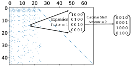
Box 1. LDPC matrix structure for 5G In this paper, we discuss LDPC for the latest standard called 5G new radio (NR) [29] by the 3rd-generation partnership project (3GPP) for wireless enhanced-mobile broadband (eMBB) communication. The 5G standard uses two base-graph (BG) matrices: BG1 and BG2, which are used to construct a parity check matrix. Fig. 3 shows the structure of BG1. The blue dots in Fig. 3 show nonzero elements of the matrix. It has 46 rows and 68 columns (BG2 matrix is 42$\times$52). Rows in the base graphs describe parity check equations. By default, BG1 generates an LDPC code with a rate equal to $1/3$, and BG2 generates an LDPC code with a rate equal to $1/5$. Figure 3: Structure of 5G-NR standard base graph 1. Each blue dot represents a nonzero element which will be replaced by a circular identity matrix based on the expansion factor as shown. Once the base graph is chosen, each zero entry is replaced with a $Z\times Z$ all-zero matrix. Each nonzero entry is replaced with a $Z\times Z$ circularly shifted identity matrix. $Z$ is called an expansion factor. The amount of circular shift depends on the value of the nonzero element. The values of the nonzero elements range from 0 to $Z-1$. If the value is 0, replace the element with the $Z\times Z$ identity matrix; otherwise, circularly shift the identity matrix based on the value. Fig. 3 shows an example with an expansion factor of 4 and a circular shift amount of 2. The 5G-NR standard allows different discrete expansion factors ranging from 2 to 384. For further details, please refer to [7].

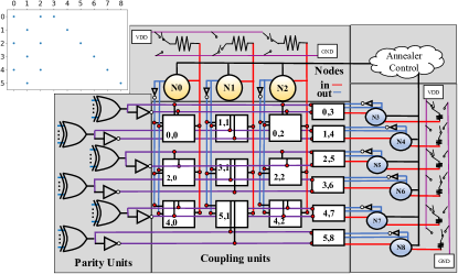
Figure 4: Illustration of our Ising machine-based LDPC decoder using a specific portion (shown in top left) of the parity check matrix.

III-C2 Structure of the matrix

As the name low-density suggests, the matrix is rather sparse, reducing the number of couplers needed. A particular property of the 5G base matrix is that a large portion of the code bits are only involved in a single parity check (so-called extension checks). In other words, many columns (representing bits) have only one non-zero element. This portion is organized as a diagonal submatrix and can be seen in Fig. 3. Because these spins have only one coupler, their couplers can be easily incorporated into their node design. Overall, the coupling array can be organized as a 2-d grid with auxiliary spins (parity checks) as one dimension regular spins as another, with the checksum bit having single parities forming a special column. The structure is shown in Fig. 4.

To recap, with this architecture, the number of couplers equals the number of 1s in the parity check matrix and is thus a constant (given a matrix), not affected by the number of auxiliary spins we added. The auxiliary spins are generated from the XOR of all bits involved in a parity check and thus have no degrees of freedom on their own. The state space of the dynamical system is only a function of the number of regular spins.

III-D Circuit design

III-D1 Nodes

In our baseline Ising machine [11], the spins are represented by voltage polarities on capacitors. When representing $\sigma_{i}=+1$, corresponding to bit $\tilde{C_{i}}=0$, the capacitor has a positive voltage. Conversely, for $\sigma_{i}=-1$, its voltage is negative.

In the circuit implementation of the proposed Ising machine, a spin is stored on a capacitor, and a node maintains the spin and interfaces with other circuits with its input/output circuit. Fig. 5 shows an initial circuit design of a node. Besides the spin capacitor, it consists of three core functional blocks: a current conveyor, a one-bit quantizer, and a pair of spin-fix (SF) switches. This node circuit takes an input current at $IN$, and generates an output voltage at $OUT$. The $OUT$ port of a node carries quantized voltage signals to both parity units and coupling units. The $IN$ port receives currents from coupling units. The node output can also be stored synchronously as a bit by an additional D flip-flop (DFF) when necessary.

The current conveyor is constructed as a class-AB current mirror [30] which is designed for high slew rate and large input dynamic range. $M_{5}$-$M_{8}$ convey the input current from port $IN$ to node $Z$, hence charging/discharging the capacitor. The two current sources $I_{bias}$ set the bias condition for $M_{1}$-$M_{4}$, and hence the operating-point voltage at $Y$ is equal to that at $X$. By biasing node $X$ to $V_{X}=1/2(V_{DD}-V_{SS})$, $V_{Y}$ is effectively biased to the same voltage. The input impedance (at port $IN$) of this circuit is low, allowing port $IN$ to operate as a current input.

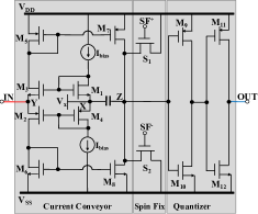
Figure 5: Circuit implementation of Node of LDPC decoder.

The capacitor’s voltage at node $Z$ represents the spin state: $V_{Z}<V_{X}$ for $\sigma_{i}=-1$, and $V_{Z}>V_{X}$ for $\sigma_{i}=+1$. Note that this voltage $V_{Z}$ is an analog signal, and needs to be quantized before it is used as an input for the XNOR gates in the parity and coupling units. Since our system operates in continuous-time, this quantizer can be simply constructed with inverters in series. In Fig. 5, $M_{9-12}$ function as both a quantizer and super-buffer.

In order to configure the system’s initial spins, two switches ($S_{1,2}$) are connected to node $Z$ to set/reset it to $V_{DD}$ or $V_{SS}$. We can also use these two switches to perform spin-fix perturbations, which allow the machine to escape local minima in search of the optimal solution. $SF_{i}^{+}$ and $SF_{i}^{-}$ are two non-overlapping control signals generated by the Annealer Control unit.

III-D2 Auxiliary spins and couplings

For the auxiliary spins represent parity checks, let us consider the concrete case of checksum $j=0$ in Eq. 9 ($\tilde{C_{1}}\oplus\tilde{C_{3}}\oplus\tilde{C_{5}}$) (the spin-based representation is $(1-\sigma_{1}\sigma_{3}\sigma_{5})/2$). The physical meaning of the coupling is quite straightforward: when $\tilde{C_{1}}\oplus\tilde{C_{3}}\oplus\tilde{C_{5}}=0$, each node will receive one unit of current keeping the node in the same polarity. Conversely, when $\tilde{C_{1}}\oplus\tilde{C_{3}}\oplus\tilde{C_{5}}=1$, each node will receive one unit of current trying to change the polarity of the node. We achieve this by generating the checksum ($\tilde{C_{1}}\oplus\tilde{C_{3}}\oplus\tilde{C_{5}}$) to select for each spin whether to couple to its positive or negative edge of its own node. An alternative view is that the selector acts as an additional XOR gate to “back out” its own node. Thus, for node 1, the coupling comes from $\tilde{C_{1}}\oplus\tilde{C_{3}}\oplus\tilde{C_{5}}\oplus\tilde{C_{1}}=\tilde{C_{3}}\oplus\tilde{C_{5}}$.

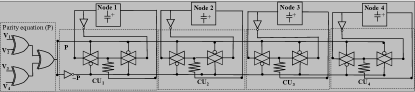
Figure 6: Circuit implementation of parity check and its coupling to spins.

III-D3 Bias

The linear terms ($-2R_{i}\sigma_{i}$ in Eq. 8) helps to constrain the decoded output closer to the received message, and is implemented by a bias current at each node proportional to the received value $R_{i}$. More specifically, according to Eq. 8, the bias current for node $i$ needs to be $\frac{4R_{i}}{\alpha}$ time that of the coupling current from the parity check. The sign of $R_{i}$ determines the polarity of the bias current.

Putting everything together, Eq. 10 describes the circuit behavior. We can see that if we use voltage $v_{i}$ (relative to virtual ground) as an approximation for spin $\sigma_{i}$ in Eq. 8, Eq. 10 is proportional to the gradient.

$$\begin{split}\derivative{v_{i}}{t}=\frac{1}{C}(I_{in})=\frac{1}{C}\left[\sum_{\mathclap{j}}J_{ij}*(P_{j\backslash i})+{J_{b}}_{i}*({v_{b}}_{i})\right]\\ \derivative{v_{i}}{t}=\frac{J}{C}(I_{in})=\frac{J}{C}\left[\frac{4R_{i}}{\alpha}*{v_{b}}_{i}+\sum_{\mathclap{H_{j,i}=1}}\sigma_{j\backslash i}\right]\end{split}$$ (10)

IV Experimental Analysis

In this section, we discuss the experimental analysis of our design by describing the experimental methodology and comparing our system to existing LDPC decoders in solution quality, throughput, and energy consumption. These decoders can be implemented using GPUs, FPGAs, or as ASICs and are often explicitly designed to a particular code. We chose 3 implementations representating the state of the art ASIC decoders for 5G standards to compare against.

Behavioral simulation of our LDPC decoder’s is done by solving Eq. 10, using MATLAB’s nonstiff, single step, 5th-order differential solver (ode45). Circuit parameters are obtained using Cadence with 45nm Generic Process Design Kit (GPDK045). We also ran a state-of-the-art variant [31] of Simulated Annealing to obtain solution quality for LDPC decoding using the traditional QUBO formulation.

IV-A Comparison with existing LDPC decoders

Table II: Comparison of the proposed LDPC decoder with existing decoders, all parameters are adjusted to implement highest expansion factor

Design\Decoder	[32]	[33]	[34]	this work
CMOS Technology	28nm	65nm	65nm	45nm
Standard	5G-NR	5G-NR	5G-NR	5G-NR
Decoding approach	Normalized Min-Sum	offset Min-Sum (OMS)	Combined Min-Sum	Augmented Ising machine
Block size	26112	26112	3808 (26112${}^{*})$	26112
Decoding Latency per iteration (nsec)	787	1530	125.33 (860${}^{*})$	320
Max Throughput per iteration (Gbs/sec)	33.2	17.06	30.38	81.6
Max Power (mW)	232	413	259	158.24
Area ($mm^{2}$)	1.97	5.74	1.49	5.44
Energy (pJ/bit) per iteration	29	24.2	8.52	1.94
quantization	5	8	4	8

*Latency scaled for direct comparison with other designs.

IV-A1 Comparison with ASIC LDPC decoders

Table II shows a detailed comparison of our work with existing ASIC LDPC decoders. The decoders are designed for 5G standards. [32], [33] support all the LDPC codes described by the 5G standards, whereas [34] is designed for a particular code created by a specific expansion factor. [34] reported their parameters for a decoder intended for an expansion factor of 56. We have modified its decoding latency to represent the decoder designed for an expansion factor of 384 by keeping area and power constant—all the other parameters are directly obtained from the corresponding papers. The table shows that our physical computation-based decoder consumes 4.4 times less energy per bit than the state of the art. Finally, earlier work using Ising machine for LDPC decoding achieves only 21Mb/s [14].

IV-B Comparison with traditional QUBO Formulation

One thousand messages were encoded using different LDPC codes to obtain the solution quality. These codes were constructed using the 5G-NR standard’s base graph 1 with varying expansion factors. The encoded messages were then modulated using BPSK modulation. Noise was added to the modulated signals based on the signal-to-noise ratio (SNR). These corrupted signals were used to test the different algorithms for solution quality.

Fig. 7 shows the solution quality of LDPC decoding using standard QUBO formulations and our proposed formulation (hybrid Ising model or modified QUBO). Since we are analyzing the quality of the formulation, we use the much faster Simulated Annealing (for 10000 iterations) to measure BER. Each message was annealed 10 times with random initializations. Fig. 7 shows the average of the bit error rate obtained. We can observe from the graphs that, given the runtime, both the formulations of QUBO yield worse BER compared to our proposed formulation.

The better performance for our formulation is part of the reason our co-designed Ising machine performs much better than earlier work using D-Wave annealer. Additionally, our proposed architecture requires far fewer couplers: 20K couplers (expansion factor 64) vs 443K and 290K couplers for unary or encoding requires respectively.

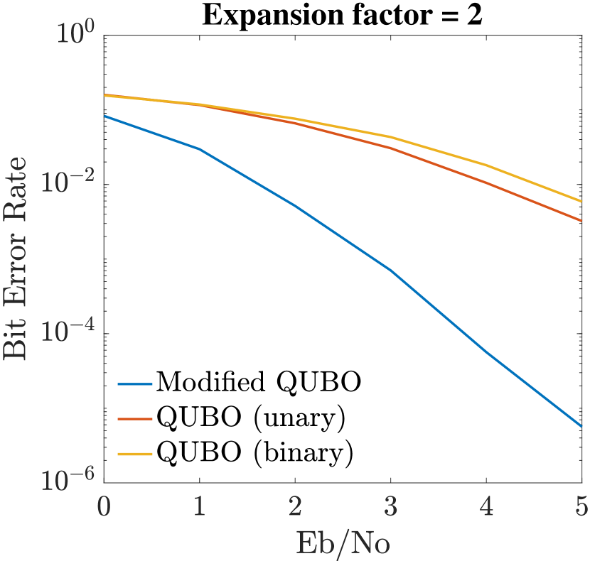
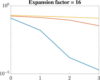
Figure 7: Bit Error Rate (BER) achieved by different algorithms at different Signal-noise ratios (Eb/No). Lower is better.

To compare the solution quality of our proposed design with different variants of belief propagation algorithm, we encoded ten thousand messages using LDPC code constructed using the 5G-NR standard’s base graph 1 with an expansion factor of 64. Fig. 8 shows the bit error rate obtained by different algorithms. ‘BP’ and ‘OMS’ in the legend represent layered Belief Propagation and layered Offset Min-Sum algorithm, respectively. BP and offset Min-sum algorithms were implemented using MATLAB’s 5G toolbox. We simulate our system evolving for 2.2 $\mu s$. The graph shows that the BER obtained by the hardware approaches the BER rate obtained by BP and its variants at the 7th iteration.

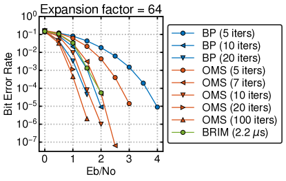
Figure 8: Bit error rate achieved by different algorithms at different Signal-to-noise ratios. Lower is better.

V Conclusions

Low density parity code (LDPC) has become the standard channel coding for many communication applications, including the 5G-NR. Fast and energy efficient LDPC decoding is thus crucial for modern communication infrastructure and the society that depends on it. The vast majority of research and prototyping efforts in decoding LDPC are focused on engineering an efficient custom circuitry hard-wiring a variant of a Belief Propagation (BP) algorithm. An alternative approach is to express the decoding as a Combinatorial Optimization Problem (COP) and leverage recent hardware advances that accelerate COP solving. However, traditional QUBO formulations of LDPC decoding require many auxiliary spins with their own degrees of freedom, thus increasing the problem state space and negatively affecting the solution quality given a fixed annealing time budget. This paper shows a new way of solving LDPC decoding by co-designing the hardware and formulation. The new approach significantly improves solution quality over traditional formulations. Enabled by a state-of-the-art Ising machine architecture, our proposed hardware is estimated to achieve a 4.4 times reduction in energy per bit compared to the most efficient decoder in literature.

References

- [1] R. W. Hamming, “Error detecting and error correcting codes,” The Bell system technical journal, vol. 29, no. 2, pp. 147–160, 1950.
- [2] A. Viterbi, “Convolutional codes and their performance in communication systems,” IEEE Transactions on Communication Technology, vol. 19, no. 5, pp. 751–772, 1971.
- [3] E. Arikan, “A performance comparison of polar codes and reed-muller codes,” IEEE Communications Letters, vol. 12, no. 6, pp. 447–449, 2008.
- [4] C. Berrou, A. Glavieux, and P. Thitimajshima, “Near shannon limit error-correcting coding and decoding: Turbo-codes. 1,” in Proceedings of ICC’93-IEEE International Conference on Communications, vol. 2. IEEE, 1993, pp. 1064–1070.
- [5] R. Gallager, “Low-density parity-check codes,” IRE Transactions on information theory, vol. 8, no. 1, pp. 21–28, 1962.
- [6] D. J. MacKay, “Good error-correcting codes based on very sparse matrices,” IEEE transactions on Information Theory, vol. 45, no. 2, pp. 399–431, 1999.
- [7] J. H. Bae, A. Abotabl, H.-P. Lin, K.-B. Song, and J. Lee, “An overview of channel coding for 5g nr cellular communications,” APSIPA Transactions on Signal and Information Processing, vol. 8, 2019.
- [8] S. Shao, P. Hailes, T.-Y. Wang, J.-Y. Wu, R. G. Maunder, B. M. Al-Hashimi, and L. Hanzo, “Survey of turbo, ldpc, and polar decoder asic implementations,” IEEE Communications Surveys & Tutorials, vol. 21, no. 3, pp. 2309–2333, 2019.
- [9] R. Maunder, “Survey of asic implementations of ldpc decoders,” 2016. [Online]. Available: https://eprints.soton.ac.uk/399259/
- [10] M. P. Fossorier, M. Mihaljevic, and H. Imai, “Reduced complexity iterative decoding of low-density parity check codes based on belief propagation,” IEEE Transactions on communications, vol. 47, no. 5, pp. 673–680, 1999.
- [11] R. Afoakwa, Y. Zhang, U. K. R. Vengalam, Z. Ignjatovic, and M. Huang, “Brim: Bistable resistively-coupled ising machine,” in 2021 IEEE International Symposium on High-Performance Computer Architecture (HPCA). IEEE, 2021, pp. 749–760.
- [12] T. Inagaki, Y. Haribara, K. Igarashi, T. Sonobe, S. Tamate, T. Honjo, A. Marandi, P. L. McMahon, T. Umeki, K. Enbutsu, O. Tadanaga, H. Takenouchi, K. Aihara, K.-i. Kawarabayashi, K. Inoue, S. Utsunomiya, and H. Takesue, “A coherent ising machine for 2000-node optimization problems,” Science, vol. 354, no. 6312, pp. 603–606, 2016.
- [13] T. Wang and J. Roychowdhury, “OIM: oscillator-based ising machines for solving combinatorial optimisation problems,” CoRR, vol. abs/1903.07163, 2019. [Online]. Available: http://arxiv.org/abs/1903.07163
- [14] S. Kasi and K. Jamieson, “Towards quantum belief propagation for ldpc decoding in wireless networks,” in Proceedings of the 26th Annual International Conference on Mobile Computing and Networking, 2020, pp. 1–14.
- [15] R. M. Karp, Reducibility among Combinatorial Problems. Boston, MA: Springer US, 1972, pp. 85–103.
- [16] A. Lucas, “Ising formulations of many np problems,” Frontiers in Physics, vol. 2, p. 5, 2014.
- [17] K. Kim, M.-S. Chang, S. Korenblit, R. Islam, E. E. Edwards, J. K. Freericks, G.-D. Lin, L.-M. Duan, and C. Monroe, “Quantum simulation of frustrated ising spins with trapped ions,” Nature, vol. 465, no. 7298, pp. 590–593, 2010.
- [18] N. G. Berloff, M. Silva, K. Kalinin, A. Askitopoulos, J. D. Töpfer, P. Cilibrizzi, W. Langbein, and P. G. Lagoudakis, “Realizing the classical xy hamiltonian in polariton simulators,” Nature materials, vol. 16, no. 11, pp. 1120–1126, 2017.
- [19] R. Barends, A. Shabani, L. Lamata, J. Kelly, A. Mezzacapo, U. Las Heras, R. Babbush, A. G. Fowler, B. Campbell, Y. Chen et al., “Digitized adiabatic quantum computing with a superconducting circuit,” Nature, vol. 534, no. 7606, pp. 222–226, 2016.
- [20] M. Yamaoka, C. Yoshimura, M. Hayashi, T. Okuyama, H. Aoki, and H. Mizuno, “A 20k-spin ising chip to solve combinatorial optimization problems with cmos annealing,” IEEE Journal of Solid-State Circuits, vol. 51, no. 1, pp. 303–309, 2015.
- [21] P. I. Bunyk, E. M. Hoskinson, M. W. Johnson, E. Tolkacheva, F. Altomare, A. J. Berkley, R. Harris, J. P. Hilton, T. Lanting, A. J. Przybysz et al., “Architectural considerations in the design of a superconducting quantum annealing processor,” IEEE Transactions on Applied Superconductivity, vol. 24, no. 4, pp. 1–10, 2014.
- [22] A. D. King, J. Carrasquilla, J. Raymond, I. Ozfidan, E. Andriyash, A. Berkley, M. Reis, T. Lanting, R. Harris, F. Altomare et al., “Observation of topological phenomena in a programmable lattice of 1,800 qubits,” Nature, vol. 560, no. 7719, pp. 456–460, 2018.
- [23] F. Böhm, G. Verschaffelt, and G. V. der Sande, “A poor man’s coherent ising machine based on opto-electronic feedback systems for solving optimization problems,” Nature communications, vol. 10, no. 1, pp. 1–9, August 2019.
- [24] R. Hamerly, A. Sludds, L. Bernstein, M. Prabhu, C. Roques-Carmes, J. Carolan, Y. Yamamoto, M. Soljačić, and D. Englund, “Towards large-scale photonic neural-network accelerators,” in 2019 IEEE International Electron Devices Meeting (IEDM). IEEE, 2019, pp. 22–8.
- [25] D. Pierangeli, G. Marcucci, and C. Conti, “Large-scale photonic ising machine by spatial light modulation,” Physical review letters, vol. 122, no. 21, p. 213902, 2019.
- [26] M. Tawada, S. Tanaka, and N. Togawa, “A new ldpc code decoding method: Expanding the scope of ising machines,” in 2020 IEEE International Conference on Consumer Electronics (ICCE). IEEE, 2020, pp. 1–6.
- [27] D-wave, “D-wave solver Properties and Parameters.” [Online]. Available: https://docs.dwavesys.com/docs/latest/c_solver_properties.html
- [28] T. Wang and J. Roychowdhury, “OIM: Oscillator-Based Ising Machines for Solving Combinatorial Optimisation Problems,” 2019.
- [29] E. TR, “5g: Study on scenarios and requirements for next generation access technologies (3gpp tr 38.913 version 14.2. 0 release 14),” ETSI TR 138 913, 2017.
- [30] S. Kawahito and Y. Tadokoro, “Cmos class-ab current mirrors for precision current-mode analog-signal-processing elements,” IEEE Transactions on Circuits and Systems II: Analog and Digital Signal Processing, vol. 43, no. 12, pp. 843–845, 1996.
- [31] S. Isakov, I. Zintchenko, T. Rønnow, and M. Troyer, “Optimised simulated annealing for ising spin glasses,” Computer Physics Communications, vol. 192, p. 265–271, Jul 2015. [Online]. Available: http://dx.doi.org/10.1016/j.cpc.2015.02.015
- [32] C.-Y. Lin, L.-W. Liu, Y.-C. Liao, and H.-C. Chang, “A 33.2 gbps/iter. reconfigurable ldpc decoder fully compliant with 5g nr applications,” in 2021 IEEE International Symposium on Circuits and Systems (ISCAS). IEEE, 2021, pp. 1–5.
- [33] S. Lee, S. Park, B. Jang, and I.-C. Park, “Multi-mode qc-ldpc decoding architecture with novel memory access scheduling for 5g new-radio standard,” IEEE Transactions on Circuits and Systems I: Regular Papers, vol. 69, no. 5, pp. 2035–2048, 2022.
- [34] T. Thi Bao Nguyen, T. Nguyen Tan, and H. Lee, “Low-complexity high-throughput qc-ldpc decoder for 5g new radio wireless communication,” Electronics, vol. 10, no. 4, p. 516, 2021.