GPS-Gaussian: Generalizable Pixel-wise 3D Gaussian Splatting for Real-time Human Novel View Synthesis

Abstract

We present a new approach, termed GPS-Gaussian, for synthesizing novel views of a character in a real-time manner. The proposed method enables 2K-resolution rendering under a sparse-view camera setting. Unlike the original Gaussian Splatting or neural implicit rendering methods that necessitate per-subject optimizations, we introduce Gaussian parameter maps defined on the source views and regress directly Gaussian Splatting properties for instant novel view synthesis without any fine-tuning or optimization. To this end, we train our Gaussian parameter regression module on a large amount of human scan data, jointly with a depth estimation module to lift 2D parameter maps to 3D space. The proposed framework is fully differentiable and experiments on several datasets demonstrate that our method outperforms state-of-the-art methods while achieving an exceeding rendering speed.

Figure 1: High-fidelity and real-time novel view synthesis (NVS). Our proposed method synthesizes $2K$-resolution novel views of unseen human performers in real-time without any fine-tuning or optimization. The performance outperforms the state-of-the-art feed-forward NVS methods ENeRF [15], FloRen [36] and 3D-GS [10], which are representative approaches in Implicit Neural Human Rendering, Image-based Human Rendering and per-subject optimization. We only mark the running efficiency for the feed-forward methods.

1 Introduction

Novel view synthesis (NVS) is a critical task that aims to produce photo-realistic images at novel viewpoints from source images captured by multi-view camera systems. Human NVS, as its subfields, could contribute to 3D/4D immersive scene capture of sports broadcasting, stage performance and holographic communication, which demands real-time efficiency and 3D consistent appearances. Previous attempts [5, 27] synthesize novel views through a weighted blending mechanism [48], but they typically rely on dense input views or precise proxy geometry. Under sparse-view camera settings, it remains a formidable challenge to render high-fidelity images for NVS.

Recently, implicit representations [34, 29, 43], especially Neural Radiance Fields (NeRF) [24], have demonstrated remarkable success in numerous NVS tasks. NeRF utilizes MLPs to represent the radiance field of the scene which jointly predicts the density and color of each sampling point. To render a specific pixel, the differentiable volume rendering technique is then implemented by aggregating a series of queried points along the ray direction. The following efforts [29, 38] in human free-view rendering immensely ease the burden of viewpoint quantities while maintaining high qualities. Despite the progress of accelerating techniques [25, 6], NVS methods with implicit representations are time-consuming in general for their dense points querying in scene space.

On the other hand, explicit representations [53, 6, 25], particularly point clouds [14, 49, 13], have drawn sustainably attention due to their high-speed, and even real-time, rendering performance. Once integrated with neural networks, point-based graphics [1, 31] realize a promising explicit representation with comparable realism and extremely superior efficiency in human NVS task [1, 31], compared with NeRF. More recently, 3D Gaussian Splatting (3D-GS) [10] introduces a new representation that the point clouds are formulated as 3D Gaussians with a series of learnable properties including 3D position, color, opacity and anisotropic covariance. By introducing $\alpha$-blending [11], 3D-GS provides not only a more reasonable and accurate mechanism for back-propagating the gradients but also a real-time rendering efficiency for complex scenes. Albeit realizing a real-time inference, Gaussian Splatting relies on per-subject [10] or per-frame [20] parameter optimizations for several minutes. It is therefore impractical in interactive scenarios as it necessitates the re-optimization of Gaussian parameters once the scene or character changes.

In this paper, we target a generalizable 3D Gaussian Splatting method to directly regress Gaussian parameters in a feed-forward manner instead of per-subject optimization. Inspired by the success of learning-based human reconstruction, PIFu-like methods [34, 35], we aim to learn the regression of human Gaussian representations from massive 3D human scan models with diverse human topologies, clothing styles and pose-dependent deformations. Deploying these learned human priors, our method enables instantaneous human appearance rendering using a generalizable Gaussian representation.

Specifically, we introduce 2D Gaussian parameter (position, color, scaling, rotation, opacity) maps which are defined on source view image planes, instead of unstructured point clouds. These Gaussian parameter maps allow us to represent a character with pixel-wise parameters, i.e. each foreground pixel corresponding to a specific Gaussian point. Additionally, it enables the application of efficient 2D convolution networks rather than expensive 3D operators. To lift 2D parameter maps to 3D Gaussian points, depth maps are estimated for both source views via two-view stereo [17] as a learnable unprojection operation. Such unprojected Gaussian points from both source views constitute the representation of character and the novel view image can be rendered with splatting technique [10].

However, the aforementioned depth estimation is not trivial to tackle with existing cascaded cost volume methods [39, 15] due to the severe self-occlusions in human characters. Therefore, we propose to learn an iterative stereo-matching [17] based depth estimation along with our Gaussian parameter regression, and jointly train the two modules on large data. Optimal depth estimation contributes to enhanced precision in determining the 3D Gaussian position, while concurrently minimizing rendering loss of Gaussian module rectifies the potential artifacts arising from the depth estimation. Such a joint training strategy benefits each component and improves the overall stability of the training process.

In practice, we are able to synthesize $2K$-resolution novel views exceeding 25 FPS on a single modern graphics card. Leveraging the rapid rendering capabilities and broad generalizability inherent in our proposed method, an unseen character can be instantly rendered without necessitating any fine-tuning or optimization, as illustrated in Fig. 1. In summary, our contributions can be summarized as follows:

• We introduce a generalizable 3D Gaussian Splatting methodology that employs pixel-wise Gaussian parameter maps defined on 2D source image planes to formulate 3D Gaussians in a feed-forward manner.

• We propose a fully differentiable framework composed of an iterative depth estimation module and a Gaussian parameter regression module. The intermediate predicted depth map bridges the two components and makes them promote mutually.

• We develop a real-time NVS system that achieves $2K$-resolution rendering by directly regressing Gaussian parameter maps.

2 Related Work

Neural Implicit Human Representation.

Neural implicit function has recently aroused a surge of interest to represent complicated scenes, in form of occupancy fields [22, 34, 35, 8], neural radiance fields [24, 29, 57, 47, 7] and neural signed distance functions [28, 43, 45, 38]. Implicit representation shows the advantage in memory efficiency and topological flexibility for human reconstruction task [8, 59, 50], especially in a pixel-aligned feature query manner [34, 35]. However, each queried point is processed through the full network, which dramatically increases computational complexity. More recently, numerous methods have extended Neural Radiance Fields (NeRF) [24] to static human modeling [37, 4] and dynamic human modeling from sparse multi-view cameras [29, 57, 38] or a monocular camera [47, 9, 7]. However, these methods typically require a per-subject optimization process and it is non-trivial to generalize these methods to unseen subjects. Previous attempts, e.g., PixelNeRF [54], IBRNet [44], MVSNeRF [3] and ENeRF [15] resort to image-based features as potent prior cues for feed-forward scene modeling. The large variation in pose and clothing makes generalizable NeRF for human rendering a more challenging task, thus recent work simplifies the problem by leveraging human priors. For example, NHP [12] and GM-NeRF [4] employ parametric human body model (SMPL [18]), KeypointNeRF uses 3D skeleton keypoints to encode spatial information, but these additional processes increase computational cost and an inaccurate prior estimation would mislead the final rendering result. On the other hand, despite the great progress in accelerating the scene-specific NeRF [53, 6, 25], efficient generalizable NeRF for interactive scenarios still remains to be further elucidated.

Deep Image-based Rendering.

Image-based rendering, or IBR in short, synthesizes novel views from a set of multi-view images with a weighted blending mechanism, which is typically computed from a geometry proxy. [32, 33] deploy multi-view stereo from dense input views to produce mesh surfaces as a proxy for image warping. DNR [41] directly produces learnable features on the surface of mesh proxies for neural rendering. Obtaining these proxies is not straightforward since high-quality multi-view stereo and surface reconstruction requires dense input views. LookinGood [21] implements RGBD fusion to attain real-time human rendering. Point clouds from SfM [23, 30] or depth sensors [26] can also be engaged as geometry proxies. These methods highly depend on the performance of 3D reconstruction algorithms or the quality of depth sensors. FWD [2] designs a network to refine depth estimations, then explicitly warps pixels from source views to novel views with the refined depth map. Several warped images are further fused to generate a final RGB image using a lightweight transformer. FloRen [36] utilizes a coarse human mesh reconstructed by PIFu [34] to render initialized depth maps for novel views. Arguably most related to ours is FloRen [36], as it also realizes $360^{\circ}$ free view human performance rendering in real-time. However, the appearance flow in FloRen merely works in 2D domains, where the rich geometry cues and multi-view geometric constraints only serve as 2D supervision. The difference is that our approach lifts 2D depth into 3D point clouds and directly utilizes the 3D point representation to render novel views in a fully differentiable manner.

Point-based Graphics.

Point-based representation has shown great efficiency and simplicity for various 3D tasks  [16, 58, 31]. Previous attempts integrate point cloud representation with 2D neural rendering [1, 31] or NeRF-like volume rendering [51], but such a hybrid architecture does not exploit rendering capability of point cloud and takes a long time to optimize each scene. Then differentiable point-based [49] and sphere-based [13] rendering have been developed, which demonstrates promising rendering results, especially attaching them to a conventional network pipeline [26]. In addition, isotropic points can be substituted by a more reasonable Gaussian point modeling [10, 20] to realize a rapid differentiable rendering with a splatting technique. However, a per-scene optimization strategy prevents it from real-world applications. In this paper, we go further to generalize 3D Gaussian Splatting across different subjects and maintain its fast and high-quality rendering properties.

3 Preliminary

Since the proposed GPS-Gaussian harnesses the power of 3D-GS [10], we give a brief introduction in this section.

3D-GS models a static 3D scene explicitly with point primitives, each of which is parameterized as a scaled Gaussian with 3D covariance matrix $\mathbf{\Sigma}$ and mean $\mathbf{\mu}$

$$G(\mathcal{X})~{}=e^{-\frac{1}{2}(\mathcal{X}-\mu)^{T}{\mathbf{\Sigma}}^{-1}(\mathcal{X}-\mu)}$$ (1)

In order to be effectively optimized by gradient descent, the covariance matrix $\mathbf{\Sigma}$ can be decomposed into a scaling matrix $\mathbf{S}$ and a rotation matrix $\mathbf{R}$ as

$$\mathbf{\Sigma}=\mathbf{RSS}^{T}\mathbf{R}^{T}$$ (2)

The projection of Gaussians from 3D space to a 2D image plane is implemented by a view transformation $\mathbf{W}$ and the Jacobian of the affine approximation of the projective transformation $\mathbf{J}$. The covariance matrix ${\mathbf{\Sigma}}^{\prime}$ in 2D space can be computed as

$$\mathbf{\Sigma^{\prime}}=\mathbf{JW\Sigma W}^{T}\mathbf{J}^{T}$$ (3)

followed by a point-based alpha-blend rendering which bears similarities to that used in NeRF [24], formulated as

$$\mathbf{C}_{color}=\sum_{i\in N}\mathbf{c}_{i}\alpha_{i}\prod_{j=1}^{i-1}(1-\alpha_{i})$$ (4)

where $\mathbf{c}_{i}$ is the color of each point, and density $\alpha_{i}$ is reasoned by the multiplication of a 2D Gaussian with covariance ${\mathbf{\Sigma}}^{\prime}$ and a learned per-point opacity [52]. The color is defined by spherical harmonics (SH) coefficients in [10].

To summarize, the vanilla 3D Gaussians methodology characterizes each Gaussian point by the following attributes: (1) a 3D position of each point $\mathcal{X}\in\mathbb{R}^{3}$, (2) a color defined by SH $\mathbf{c}\in\mathbb{R}^{k}$ (where $k$ is the freedom of SH basis), (3) a rotation parameterized by a quaternion $\mathbf{r}\in\mathbb{R}^{4}$, (4) a scaling factor $\mathbf{s}\in\mathbb{R}_{+}^{3}$, and (5) an opacity $\alpha\in[0,1]$.

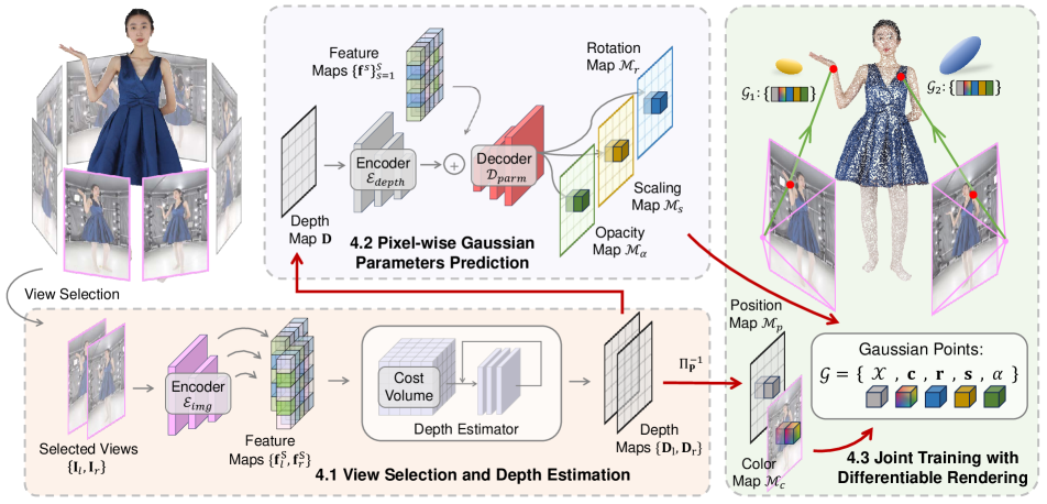
Figure 2: Overview of GPS-Gaussian. Given RGB images of a human-centered scene with sparse camera views and a target novel viewpoint, we select the adjacent two views on which to formulate our Gaussian representation. We extract the image features followed by conducting an iterative depth estimation. For each source view, the depth map and the RGB image serve as a 3D position map and a color map, respectively, to formulate the Gaussian representation while the other parameters of 3D Gaussians are predicted in a pixel-wise manner. The Gaussian parameter maps defined on 2D image planes of both views are further unprojected to 3D space and aggregated for novel view rendering. The fully differentiable framework enables all networks a joint training mechanism.

4 Method

The overview of our method is illustrated in Fig. 2. Given the RGB images of a human-centered scene with sparse camera views, our method aims to generate high-quality free-viewpoint renderings of the performer in real-time. Once given a target novel viewpoint, we select the two neighboring views and extract the image features using a shared image encoder. Following this, a two-view depth estimator takes the extracted features as input to predict the depth maps for both source views (Sec. 4.1). The depth values and the RGB values in foreground regions of the source view determine the 3D position and color of each Gaussian point, respectively, while the other parameters of 3D Gaussians are predicted in a pixel-wise manner (Sec. 4.2). Combined with the depth map and source RGB image, these parameter maps formulate the Gaussian representation in 2D image planes and are further unprojected to 3D space. The unprojected Gaussians from both views are aggregated and rendered to the target viewpoint in a differentiable way, which allows for end-to-end training (Sec. 4.3).

4.1 View Selection and Depth estimation

View Selection. Unlike the vanilla 3D Gaussians that optimize the characteristics of each Gaussian point on all source views, we synthesize the novel target view by interpolating the adjacent two source views. Given the $N$ input images denoted as $\{\mathbf{I}_{n}\}_{n=1}^{N}$, with their camera position $\{C_{n}\}_{n=1}^{N}$, the source views can be represented by $\mathbf{V_{n}}=C_{n}-O$, where $O$ is the center of the scene. Similarly, the target novel view rendering can be defined as $I_{tar}$ with target camera position $C_{tar}$ and view $\mathbf{V_{tar}}=C_{tar}-O$. By conducting a dot product of the input views vectors and the novel view vector, we can select the nearest two views $(v_{l},v_{r})$ as the ‘working set’ of two-view stereo, where $l$ and $r$ stand for ‘left’ and ‘right’ view, respectively.

The rectified source images $\mathbf{I}_{l},\mathbf{I}_{r}\in[0,1]^{H\times W\times 3}$ are fed to a shared image encoder $\mathcal{E}_{img}$ with several residual blocks and downsampling layers to extract dense feature maps $\mathbf{f}^{s}\in\mathbb{R}^{H/2^{s}\times W/2^{s}\times D_{s}}$ where $D_{s}$ is the dimension at the $s$-th feature scale

$$\langle\{\mathbf{f}_{l}^{s}\}_{s=1}^{S},\{\mathbf{f}_{r}^{s}\}_{s=1}^{S}\rangle=\mathcal{E}_{img}(\mathbf{I}_{l},\mathbf{I}_{r})$$ (5)

where we set $S=3$ in our experiments.

Depth Estimation. The depth map is the key component of our framework bridging the 2D image planes and 3D Gaussian representation. Note that, depth estimation in two-view stereo is equivalent to disparity estimation. For each pixel $(u,v)$ in one view, disparity estimation $\phi_{disp}$ aims to find its corresponding coordinate $(u+\phi_{disp}(u),v)$ in another view, considering the displacement of each pixel is constrained to a horizontal line in rectified stereo. Since disparity predictions can be easily converted to depth maps given camera parameters, we do not distinguish between depth maps and disparity maps in the following sections. In theory, any alternative depth estimation methods can be adapted to our framework. We implement this module in an iterative manner inspired by [17] mainly because it avoids using prohibitively slow 3D convolutions to filter the cost volume.

Given the feature maps $\mathbf{f}_{l}^{S},\mathbf{f}_{r}^{S}\in\mathbb{R}^{H/2^{S}\times W/2^{S}\times D_{S}}$, we compute a 3D correlation volume $\mathbf{C}\in\mathbb{R}^{H/2^{S}\times W/2^{S}\times W/2^{S}}$ using a matrix multiplication

$$\mathbf{C}(\mathbf{f}_{l}^{S},\mathbf{f}_{r}^{S}),\quad C_{ijk}=\sum_{h}(\mathbf{f}_{l}^{S})_{ijh}\cdot(\mathbf{f}_{r}^{S})_{ikh}\vspace{-2mm}$$ (6)

Then, an iterative update mechanism predicts a sequence of depth estimations $\{\mathbf{d}_{l}^{t}\}_{t=1}^{T}$ and $\{\mathbf{d}_{r}^{t}\}_{t=1}^{T}$ by looking up in volume $\mathbf{C}$, where $T$ is the number of update times. For more details about the update operators, please refer to [40]. The outputs of final iterations ($\mathbf{d}_{l}^{T}$, $\mathbf{d}_{r}^{T}$) are upsampled to a full-resolution image size via a convex upsampling. The depth estimation module $\Phi_{depth}$ can be formulated as

$$\langle\mathbf{D}_{l},\mathbf{D}_{r}\rangle=\Phi_{depth}(\mathbf{f}_{l}^{S},\mathbf{f}_{r}^{S},K_{l},K_{r})$$ (7)

where $K_{l}$ and $K_{r}$ are the camera parameters, $\mathbf{D}_{l},\mathbf{D}_{r}\in\mathbb{R}^{H\times W\times 1}$ are the depth estimations. The classic two-view stereo methods estimate the depth for ‘reference views’ only, while we pursue depth maps of both inputs to formulate the Gaussian representation, which makes our implementation highly symmetrical. By leveraging this nature, we realize a compact and highly parallelized module that results in a decent efficiency increase. Detailed designs of this module can be seen in our supplementary material.

4.2 Pixel-wise Gaussian Parameters Prediction

Each Gaussian point in 3D space is characterized by attributes $\mathcal{G}=\{\mathcal{X},\mathbf{c},\mathbf{r},\mathbf{s},\alpha\}$, which represent 3D position, color, rotation, scaling and opacity, respectively. In this section, we introduce a pixel-wise manner to formulate 3D Gaussians in 2D image planes. Specifically, we formulate our Gaussian maps $\mathbf{G}$ as

$$\mathbf{G}(x)=\{\mathcal{M}_{p}(x),\mathcal{M}_{c}(x),\mathcal{M}_{r}(x),\mathcal{M}_{s}(x),\mathcal{M}_{\alpha}(x)\}$$ (8)

where $x$ is the coordinate of a foreground pixel in an image plane, $\mathcal{M}_{p},\mathcal{M}_{c},\mathcal{M}_{r},\mathcal{M}_{s},\mathcal{M}_{\alpha}$ represents Gaussian parameter maps of position, color, rotation, scaling and opacity, respectively. Given the predicted depth map $\mathbf{D}$, a pixel located at $x$ can be immediately unprojected from image planes to 3D space using projection matrix $\mathbf{P}\in\mathbb{R}^{3\times 4}$ structure with camera parameters $K$

$$\mathcal{M}_{p}(x)=\Pi^{-1}_{\mathbf{P}}(x,\mathbf{D}(x))$$ (9)

Thus the learnable unprojection in Eq. 9 bridges 2D feature space and 3D Gaussian representation. Considering our human-centered scenario is predominantly characterized by diffuse reflection, instead of predicting the SH coefficients, we directly use the source RGB image as the color map

$$\mathcal{M}_{c}(x)=\mathbf{I}(x)\vspace{-1mm}$$ (10)

We argue that the remaining three Gaussian parameters are generally related to (1) pixel level local features, (2) a global context of human bodies, and (3) a detailed spatial structure. Image features $\{\mathbf{f}^{s}\}_{s=1}^{S}$ from encoder $\mathcal{E}_{img}$ have already derived strong cues of (1) and (2). Hence, we construct an additional encoder $\mathcal{E}_{depth}$ that has an identical architecture to the image encoder and takes the depth map D as input. Depth features complement the geometric awareness for each pixel for better Gaussian parameters reasoning. The image features and the spatial features are fused by a U-Net like decoder $\mathcal{D}_{parm}$ to regress pixel-wise Gaussian features in full image resolution

$$\mathbf{\Gamma}=\mathcal{D}_{parm}(\mathcal{E}_{img}(\mathbf{I})\oplus\mathcal{E}_{depth}(\mathbf{D}))$$ (11)

where $\mathbf{\Gamma}\in\mathbb{R}^{H\times W\times D_{G}}$, $D_{G}$ is the dimension of Gaussian features, $\oplus$ stands for concatenations at all feature levels. The prediction heads, each composed of 2 convolution layers, are adapted to Gaussian features for specific Gaussian parameter map regression. Before being used to formulate Gaussian representations, the rotation map should be normalized since it represents a quaternion

$$\mathcal{M}_{r}(x)=Norm({h}_{r}(\mathbf{\Gamma}(x)))\vspace{-1mm}$$ (12)

where ${h}_{r}$ is the rotation head. The scaling map and the opacity map need activations to satisfy their range

$$\begin{split}\mathcal{M}_{s}(x)=Softplus({h}_{s}(\mathbf{\Gamma}(x)))\\ \mathcal{M}_{\alpha}(x)=Sigmoid({h}_{\alpha}(\mathbf{\Gamma}(x)))\end{split}$$ (13)

where ${h}_{s}$ and ${h}_{\alpha}$ represent the scaling head and opacity head, respectively. The detailed network architecture in this section is provided in our supplementary materials.

Table 1: Qualitative comparison on THuman2.0 [55], Twindom [42] and our collected real-world data. All methods are evaluated on an RTX 3090 GPU to report the speed of rendering a 1024 × 1024 image. $\dagger$ Unlike other methods, 3D-GS [10] necessitates a per-subject optimization, while the others can perform feed-forward inferences.

Method	THuman2.0 [55]			Twindom [42]			Real-world Data			FPS
	PSNR$\uparrow$	SSIM$\uparrow$	LPIPS$\downarrow$	PSNR$\uparrow$	SSIM$\uparrow$	LPIPS$\downarrow$	PSNR$\uparrow$	SSIM$\uparrow$	LPIPS$\downarrow$
3D-GS [10]$\dagger$	24.18	0.821	0.144	22.77	0.785	0.153	22.97	0.839	0.125	/
FloRen [36]	23.26	0.812	0.184	22.96	0.838	0.165	22.80	0.872	0.136	15
IBRNet [44]	23.38	0.836	0.212	22.92	0.803	0.238	22.63	0.852	0.177	0.25
ENeRF [15]	24.10	0.869	0.126	23.64	0.847	0.134	23.26	0.893	0.118	5
Ours	25.57	0.898	0.112	24.79	0.880	0.125	24.64	0.917	0.088	25

4.3 Joint Training with Differentiable Rendering

The pixel-wise Gaussian parameter maps defined on both of the two source views are lifted to 3D space and aggregated to render a photo-realistic novel view image using Gaussian Splatting in Sec. 3.

Joint Training Mechanism. The fully differentiable rendering framework simultaneously enables joint training from two perspectives: (1) The depth estimations of both source views. (2) The depth estimation module and the Gaussian parameter prediction module. As for the former, the independent training of depth estimators on two source views could make the 3D representation inconsistent due to the slight mismatch of the source views. As for the latter, the classic stereo-matching based depth estimation is fundamentally a 2D task that aims at densely finding the correspondence between pixels from two images, the differentiable rendering integrates auxiliary 3D awareness to promote this issue. On the other hand, optimal depth estimation contributes to enhanced precision in determining the 3D Gaussian parameters.

Loss Functions. We use L1 loss and SSIM loss [46], denoted as $\mathcal{L}_{mae}$ and $\mathcal{L}_{ssim}$ respectively, to measure the difference between the rendered and ground truth image

$$\mathcal{L}_{render}=\beta{L}_{mae}+\gamma\mathcal{L}_{ssim}$$ (14)

where we set $\beta=0.8$ and $\gamma=0.2$ in our experiments. Similar to [17], we supervise on the L1 distance between the predicted and ground truth depth over the full sequence of predictions $\{\mathbf{d}^{t}\}_{t=1}^{T}$ with exponentially increasing weights. Given ground truth depth $\mathbf{d}_{gt}$, the loss is defined as

$$\mathcal{L}_{disp}=\sum_{t=1}^{T}\mu^{T-t}\|\mathbf{d}_{gt}-\mathbf{d}^{t}\|_{1}$$ (15)

where we set $\mu=0.9$ in our experiments. Our final loss function is $\mathcal{L}=\mathcal{L}_{render}+\mathcal{L}_{disp}$.

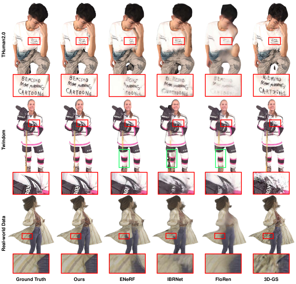
Figure 3: Qualitative comparison on THuman2.0 [55], Twindom [42] and our collected real-world data. Our method produces more detailed human appearances and can recover more reasonable geometry.

5 Experiments

5.1 Implementation Details

Our GPS-Gaussian is trained on a single RTX3090 graphics card using AdamW [19] optimizer with an initial learning rate of $2e^{-4}$. Since the unstable depth estimation in the very first training steps can have a strong impact on Gaussian parameter regression, we pre-train the depth estimation module for $40k$ iterations. Then we jointly train two modules for $100k$ iterations with a batch size of $2$ and the whole training process takes around 15 hours.

5.2 Datasets and Metrics

To learn human priors from a large amount of data, we collect 1700 and 526 human scans from Twindom [42] and THuman2.0 [55], respectively. We randomly select 200 and 100 scans as validation data from Twindom and THuman2.0, respectively. As shown in Fig. 2, we uniformly position 8 cameras in a cycle, thus the angle between two neighboring cameras is about $45^{\circ}$. We render synthetic human scans to these camera positions as source view images while randomly choosing 3 viewpoints to render novel view images, which are positioned on the intersection arc between each two adjacent input views. To test the robustness in real-world scenarios, we capture real data of 4 characters in the same 8-camera setting and prepare 8 additional camera views as evaluation data. Similar to ENeRF [15], we evaluate PSNR, SSIM [46] and LPIPS [56] as metrics for the rendering results in foreground regions determined by the bounding box of humans.

5.3 Comparisons with State-of-the-art Methods

Baselines. Considering that our goal is instant NVS rendering, we compare our GPS-Gaussian against three generalizable methods including implicit method ENeRF [15], Image-based rendering method FloRen [36] and hybrid method IBRNet [44]. All baseline methods are trained from scratch on the same dataset as ours and take as input two source views for one novel view rendering, the same setting as ours, at each training iteration. We further prepare the comparison with one per-subject optimization method 3D-GS [10] which is optimized on all 8 input views using the default strategies in the released code.

Comparison Results. We prepare comparisons on both synthetic data and real-world data. In Table 1, our GPS-Gaussian outperforms all methods on all metrics and achieves a much faster rendering speed. For qualitative rendering results shown in Fig. 3, our method is able to synthesize fine-grained novel view images with more detailed appearances. Once occlusion happens, some target regions under the novel view are invisible in one or both of source views. In this case, depth ambiguity between input views causes ENeRF and IBRNet to render unreasonable results since these methods are confused when conducting the feature aggregation. The unreliable geometric proxy in these cases also makes FloRen produce blurred outputs even if it employs the depth and flow refining networks. In our method, the human priors learned from massive human images help to alleviate the adverse effects caused by occlusion. In addition, 3D-GS takes several minutes for optimization and produces noisy rendering results of novel views in such a sparse camera setting. Also, most of the compared methods have difficulty in handling thin structures such as hockey sticks and robes in Fig. 3. We further prepare the sensitivity analysis of camera view sparsity in Table 2. For the results of 6-camera, we use the same model trained in 8-camera setting without any fine-tuning. Among baselines, our method degrades reasonably and holds robustness when decreasing cameras. We ignore 3D-GS here because it takes several minutes per-subject optimization and produces noisy rendering results, as shown in Fig. 3, even in 8-camera setting.

Table 2: Sensibility to camera sparsity. We use the model trained on an 8-camera setting to perform inference on a 6-camera setting.

Model	8 cameras			6 cameras
	PSNR$\uparrow$	SSIM$\uparrow$	LPIPS$\downarrow$	PSNR$\uparrow$	SSIM$\uparrow$	LPIPS$\downarrow$
FloRen [36]	23.26	0.812	0.184	18.72	0.770	0.267
IBRNet [44]	23.38	0.836	0.212	21.08	0.790	0.263
ENeRF [15]	24.10	0.869	0.126	21.78	0.831	0.181
Ours	25.57	0.898	0.112	23.03	0.884	0.168

5.4 Ablation Studies

We evaluate the effectiveness of our designs in more detail through ablation experiments. Other than rendering metrics, we follow [17] to evaluate depth (identical to disparity) estimation with the end-point-error (EPE) and the ratio of pixel error in 1 pix level. All ablations are trained and tested on the aforementioned synthetic data.

Table 3: Quantitative ablation study on synthetic data. We report PSNR, SSIM and LPIPS metrics for evaluating the rendering quality, while the end-point-error (EPE) and the ratio of pixel error in 1 pix level for measuring depth accuracy.

Model	Rendering			Depth
	PSNR$\uparrow$	SSIM$\uparrow$	LPIPS$\downarrow$	EPE $\downarrow$	1 pix $\uparrow$
Full model	25.05	0.886	0.121	1.494	65.94
w/o Joint Train.	23.97	0.862	0.115	1.587	63.71
w/o Depth Enc.	23.84	0.858	0.204	1.496	65.87

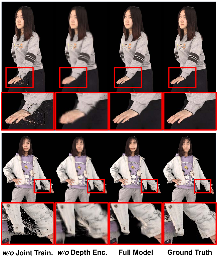
Figure 4: Qualitative ablation study on synthetic data. We show the effectiveness of the joint training and the depth encoder in the full pipeline. The proposed designs make the rendering results more visually appealing with fewer artifacts and less blurry.

Effects of Joint Training Mechanism. We design a model without the differentiable Gaussian rendering by substituting it with point cloud rendering at a fixed radius. Thus the model degenerates into a depth estimation network and an undifferentiable depth warping based rendering. The rendering quality is merely based on the accuracy of depth estimation while the rendering loss could not conversely promote the depth estimator. We train the ablated model for the same iterations as the full model for fair comparison. The rendering results in Fig. 4 witness obvious noise due to the depth ambiguity in the margin area of the source views where the depth value changes drastically. The rendering noise causes a degradation in PSNR and SSIM as manifested in Table 3, while cannot be reflected in the perception matric LPIPS. The joint regression with Gaussian parameters precisely recognizes these outliers and compensates for these artifacts by predicting an extremely low opacity for the Gaussian points centered at these points. Meanwhile, the independent training of the depth estimation module interrupts the interaction of two source views, resulting in an inconsistency when recovering the geometry. As illustrated in Table 3, joint learning makes a more robust depth estimator with a $5\%$ improvement in EPE.

Effects of Depth Encoder. We claim that merely using image features is insufficient for predicting Gaussian parameters. Herein, we remove the depth encoder from our full model, thus the Gaussian parameter decoder only takes as input the image features to predict $\mathcal{M}_{r},\mathcal{M}_{s},\mathcal{M}_{\alpha}$ simultaneously. As shown in Fig. 4, we find the model fails to recover the details of human appearance, leading to blurred rendering results. The absence of spatial awareness makes the predicted Scaling Map $\mathcal{M}_{s}$ incline to a mean value, which causes serious overlaps between Gaussian points. This drawback significantly deteriorates the visual perception reflected on the LPIPS, even with a comparable depth estimation accuracy, as shown in Table 3.

6 Conclusion and Discussion

By regressing directly Gaussian parameter maps defined on the estimated depth images of source views, our GPS-Gaussian takes a significant step towards real-time and photo-realistic Novel View Synthesis system using only sparse view cameras. Our proposed pipeline is fully differentiable and carefully designed. We demonstrate that our method improves notably both quantitative and qualitative results compared with baseline methods and achieves a much faster rendering speed on a single RTX 3090 GPU.

Although the proposed GPS-Gaussian synthesizes high-quality images, some elements can still impact the effectiveness of our method. For example, an accurate foreground matting is necessary as preprocessing step. Besides, we can not perfectly handle a very large disparity in the case of 6-camera setting when a target region in one view is totally invisible in another view. We believe that one can leverage temporal information to solve this problem.

Supplementary Material

In this supplementary material, we present the run-time comparison (Sec. A), visualization of opacity maps (Sec. B), the details of network architecture (Sec. C) and live demo (Sec. D).

Appendix A Run-time Comparison

We compare the run-time of the proposed GPS-Gaussian with baseline methods. All compared methods generally contain two components including view independent computation on input source images and a target view orientated rendering which depends on the given novel viewpoint. The detailed run-time of each method on both contents is illustrated in Table A. The view independent computation in FloRen [36] contains matting and coarse geometry initialization while the key component including the depth and flow refinement networks operates on novel viewpoints. IBRNet [44] uses transformers to aggregate multi-view cues at each sampling point of novel view direction, which makes view dependent computation time-consuming. ENeRF [15] constructs two view dependent cost volumes in a coarse-to-fine manner to predict the depth of the target viewpoint followed by a depth-guided sampling for volume rendering. These methods necessitate recomputations of the view dependent modules once the target viewpoint changes. In our GPS-Gaussian, the main computation lies on Gaussian parameter map regression and depth estimation, which are formulated on source image planes. The unprojected Gaussian representation from source views enables 3D consistent novel view rendering. Given a target viewpoint, it takes only 0.8 ms to render the 3D Gaussians to the target 2D image plane. This allows us to render multiple images simultaneously given the viewpoints of multiple viewers.

Table A: Run-time comparison. ‘View independent’ computation refers to the network latency on source views. ‘View dependent’ computation refers to the view-specific inference on a single novel viewpoint. The rendering resolution here is set to $1024\times 1024$. The proposed Gaussian parameter maps are completely formulated on source views, while the only novel view dependent manipulation in our method is the Gaussian Splatting rendering. The fast view dependent computation speed of our method enables novel view synthesis for multiple viewpoints immediately in real-time.

Methods	View independent	View dependent (per view)
FloRen [36]	14 ms	11 ms
IBRNet [44]	5 ms	4000 ms
ENeRF [15]	11 ms	125 ms
Ours	27 ms	0.8 ms

Appendix B Visualization of Opacity Maps

As mentioned in Sec. 5.4, the joint regression with Gaussian parameters eliminates the outliers by predicting an extremely low opacity for the Gaussian points centered at these points. The visualization of opacity maps is shown in Fig. A. Since the depth prediction works on low resolution and upsampled to full-image size, the drastically changed depth in the margin areas causes ambiguous predictions (e.g. the front and rear placed legs of the girl and the crossed arms of the boy in Fig. A). These ambiguities further lead to rendering noise on novel views when using a point cloud rendering technique. Thanks to the learned opacity map, the predicted low opacity values make the outliers invisible in the final novel view rendering results, as shown in Fig. A (e).

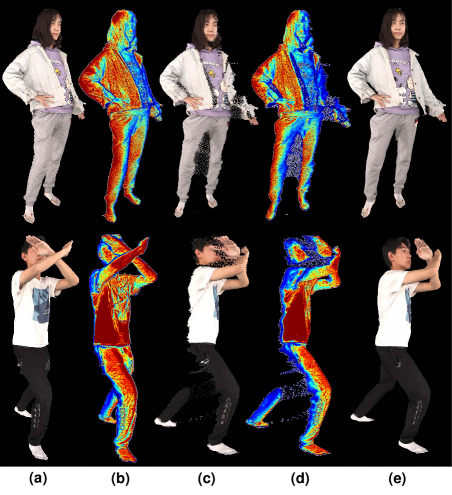
Figure A: Visualization of opacity maps. (a) One of the source view images. (b) The predicted opacity map related to (a). (c)/(d) The projected color/opacity map from the source view to the novel viewpoint. (e) The novel view rendering result. The opacity values are visualized in the heat map where a cold color represents a value near 0, and a hot color represents a value near 1. The low opacity values predicted for the outliers make them invisible in the rendering results.

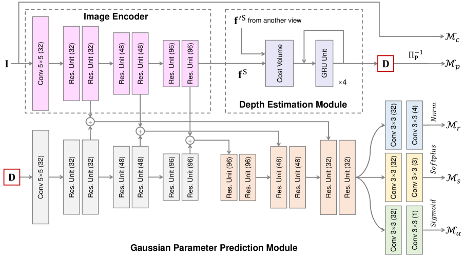
Figure B: Network architecture. The proposed framework takes the source image as input to regress the Gaussian parameter maps (color map $\mathcal{M}_{c}$, position map $\mathcal{M}_{p}$, rotation map $\mathcal{M}_{r}$, scaling map $\mathcal{M}_{s}$ and opacity map $\mathcal{M}_{\alpha}$).

Appendix C Network Architecture

The network architecture of the proposed GPS-Gaussian is shown in Fig. B. The framework is composed of three modules including (1) image encoder, (2) depth estimation module, and (3) Gaussian parameter prediction module.

Image Encoder. The image encoder $\mathcal{E}_{img}$ is applied to both the left and right images and maps each image to a set of dense feature map $\{\mathbf{f}_{l}^{s}\}_{s=1}^{S}$ as in Eq. 5. The image encoder $\mathcal{E}_{img}$ has a similar architecture to the feature encoder in RAFT-Stereo [17]. We replace the $7\times 7$ convolution with a $5\times 5$ one at the beginning of the network and replace all batch normalization with group normalization. Residual blocks and downsampling layers are used to produce image features in 3 levels at $1/2$, $1/4$ and $1/8$ the input image resolution, with $32$, $48$ and $96$ channels, respectively. The extracted features are further used to construct the correlation volume and regress the Gaussian parameters.

Depth Estimation Module. As mentioned in Sec. 4.1, The classic two-view stereo methods estimate the depth for ‘reference view’ only, while the feature of ‘target view’ is only used to construct the cost volume but not involved in the further depth estimation or iterative refine module. The cost volume in Eq. 6 is computed redundantly if exchanging the role of both inputs for depth estimation of both views. By making the image encoder independent from the disparity estimation module, and re-indexing the correlation volume $\mathbf{C}$ for both lookup procedures, we realize a compact and highly parallelized implementation that results in a decent efficiency increase exceeding 30%. For the refinement module, we set $T=4$ considering the trade-off between the performance and the cost. The GRU units are identical to that implemented in RAFT-Stereo [17].

Gaussian Parameter Prediction Module. This module is composed of a depth encoder $\mathcal{E}_{img}$ and a U-Net like Gaussian parameter decoder $\mathcal{D}_{parm}$. The depth encoder, which takes as input the depth prediction, has an identical architecture to the image encoder. Image features and depth features are concatenated at each level and further aggregated to the Gaussian parameter decoder via skip connections. The decoded pixel-wise Gaussian feature $\mathbf{\Gamma}$ passes through three specific prediction heads to get rotation map $\mathcal{M}_{r}$, scaling map $\mathcal{M}_{s}$ and opacity map $\mathcal{M}_{\alpha}$, respectively. Meanwhile, the position map $\mathcal{M}_{p}$ is determined by the predicted depth map D and the color map $\mathcal{M}_{c}$ directly borrows from the RGB value of the input image.

Appendix D Live Demo

We prepare a live demo in supplementary video, in which we capture source view RGB streams and render novel view in one system. Due to the memory cost of RTX 3090, we connect the front 6 cameras faced human subjects to the computer, and cameras are positioned in a circle of a 2-meter radius. We note that our method achieves high-quality real-time rendering, even for challenging hairstyles and human-object interaction.

References

- Aliev et al. [2020] Kara-Ali Aliev, Artem Sevastopolsky, Maria Kolos, Dmitry Ulyanov, and Victor Lempitsky. Neural point-based graphics. In ECCV, pages 696–712. Springer, 2020.
- Cao et al. [2022] Ang Cao, Chris Rockwell, and Justin Johnson. Fwd: Real-time novel view synthesis with forward warping and depth. In CVPR, pages 15713–15724, 2022.
- Chen et al. [2021] Anpei Chen, Zexiang Xu, Fuqiang Zhao, Xiaoshuai Zhang, Fanbo Xiang, Jingyi Yu, and Hao Su. Mvsnerf: Fast generalizable radiance field reconstruction from multi-view stereo. In ICCV, pages 14124–14133, 2021.
- Chen et al. [2023] Jianchuan Chen, Wentao Yi, Liqian Ma, Xu Jia, and Huchuan Lu. Gm-nerf: Learning generalizable model-based neural radiance fields from multi-view images. In CVPR, pages 20648–20658, 2023.
- Chen and Williams [1993] Shenchang Eric Chen and Lance Williams. View interpolation for image synthesis. In Conference on Computer Graphics and Interactive Techniques. 1993.
- Fridovich-Keil et al. [2022] Sara Fridovich-Keil, Alex Yu, Matthew Tancik, Qinhong Chen, Benjamin Recht, and Angjoo Kanazawa. Plenoxels: Radiance fields without neural networks. In CVPR, pages 5501–5510, 2022.
- Guo et al. [2023] Chen Guo, Tianjian Jiang, Xu Chen, Jie Song, and Otmar Hilliges. Vid2avatar: 3d avatar reconstruction from videos in the wild via self-supervised scene decomposition. In CVPR, pages 12858–12868, 2023.
- Hong et al. [2021] Yang Hong, Juyong Zhang, Boyi Jiang, Yudong Guo, Ligang Liu, and Hujun Bao. Stereopifu: Depth aware clothed human digitization via stereo vision. In CVPR, pages 535–545, 2021.
- Jiang et al. [2022] Wei Jiang, Kwang Moo Yi, Golnoosh Samei, Oncel Tuzel, and Anurag Ranjan. Neuman: Neural human radiance field from a single video. In ECCV, pages 402–418. Springer, 2022.
- Kerbl et al. [2023] Bernhard Kerbl, Georgios Kopanas, Thomas Leimkühler, and George Drettakis. 3d gaussian splatting for real-time radiance field rendering. ACM TOG, 42(4):1–14, 2023.
- Kopanas et al. [2022] Georgios Kopanas, Thomas Leimkühler, Gilles Rainer, Clément Jambon, and George Drettakis. Neural point catacaustics for novel-view synthesis of reflections. ACM TOG, 41(6), 2022.
- Kwon et al. [2021] Youngjoong Kwon, Dahun Kim, Duygu Ceylan, and Henry Fuchs. Neural human performer: Learning generalizable radiance fields for human performance rendering. NeurIPS, 34:24741–24752, 2021.
- Lassner and Zollhofer [2021] Christoph Lassner and Michael Zollhofer. Pulsar: Efficient sphere-based neural rendering. In CVPR, pages 1440–1449, 2021.
- Levoy and Whitted [1985] Marc Levoy and Turner Whitted. The use of points as a display primitive. 1985.
- Lin et al. [2022a] Haotong Lin, Sida Peng, Zhen Xu, Yunzhi Yan, Qing Shuai, Hujun Bao, and Xiaowei Zhou. Efficient neural radiance fields for interactive free-viewpoint video. In SIGGRAPH Asia 2022 Conference Papers, pages 1–9, 2022a.
- Lin et al. [2022b] Siyou Lin, Hongwen Zhang, Zerong Zheng, Ruizhi Shao, and Yebin Liu. Learning implicit templates for point-based clothed human modeling. In ECCV, pages 210–228. Springer, 2022b.
- Lipson et al. [2021] Lahav Lipson, Zachary Teed, and Jia Deng. Raft-stereo: Multilevel recurrent field transforms for stereo matching. In 3DV, pages 218–227. IEEE, 2021.
- Loper et al. [2015] Matthew Loper, Naureen Mahmood, Javier Romero, Gerard Pons-Moll, and Michael J Black. Smpl: A skinned multi-person linear model. ACM TOG, 34(6):1–16, 2015.
- Loshchilov and Hutter [2019] Ilya Loshchilov and Frank Hutter. Decoupled weight decay regularization. In ICLR. OpenReview.net, 2019.
- Luiten et al. [2024] Jonathon Luiten, Georgios Kopanas, Bastian Leibe, and Deva Ramanan. Dynamic 3d gaussians: Tracking by persistent dynamic view synthesis. In 3DV, 2024.
- Martin-Brualla et al. [2018] Ricardo Martin-Brualla, Rohit Pandey, Shuoran Yang, Pavel Pidlypenskyi, Jonathan Taylor, Julien Valentin, Sameh Khamis, Philip Davidson, Anastasia Tkach, Peter Lincoln, et al. Lookingood: enhancing performance capture with real-time neural re-rendering. ACM TOG, 37(6):1–14, 2018.
- Mescheder et al. [2019] Lars Mescheder, Michael Oechsle, Michael Niemeyer, Sebastian Nowozin, and Andreas Geiger. Occupancy networks: Learning 3d reconstruction in function space. In CVPR, pages 4460–4470, 2019.
- Meshry et al. [2019] Moustafa Meshry, Dan B Goldman, Sameh Khamis, Hugues Hoppe, Rohit Pandey, Noah Snavely, and Ricardo Martin-Brualla. Neural rerendering in the wild. In CVPR, pages 6878–6887, 2019.
- Mildenhall et al. [2020] Ben Mildenhall, Pratul P Srinivasan, Matthew Tancik, Jonathan T Barron, Ravi Ramamoorthi, and Ren Ng. Nerf: Representing scenes as neural radiance fields for view synthesis. In ECCV, pages 405–421. Springer, 2020.
- Müller et al. [2022] Thomas Müller, Alex Evans, Christoph Schied, and Alexander Keller. Instant neural graphics primitives with a multiresolution hash encoding. ACM TOG, 41(4), 2022.
- Nguyen-Ha et al. [2022] Phong Nguyen-Ha, Nikolaos Sarafianos, Christoph Lassner, Janne Heikkilä, and Tony Tung. Free-viewpoint rgb-d human performance capture and rendering. In ECCV, pages 473–491. Springer, 2022.
- Oh et al. [2001] Byong Mok Oh, Max Chen, Julie Dorsey, and Frédo Durand. Image-based modeling and photo editing. In Proceedings of the 28th annual conference on Computer graphics and interactive techniques, pages 433–442, 2001.
- Park et al. [2019] Jeong Joon Park, Peter Florence, Julian Straub, Richard Newcombe, and Steven Lovegrove. Deepsdf: Learning continuous signed distance functions for shape representation. In CVPR, pages 165–174, 2019.
- Peng et al. [2021] Sida Peng, Yuanqing Zhang, Yinghao Xu, Qianqian Wang, Qing Shuai, Hujun Bao, and Xiaowei Zhou. Neural body: Implicit neural representations with structured latent codes for novel view synthesis of dynamic humans. In CVPR, pages 9054–9063, 2021.
- Pittaluga et al. [2019] Francesco Pittaluga, Sanjeev J Koppal, Sing Bing Kang, and Sudipta N Sinha. Revealing scenes by inverting structure from motion reconstructions. In CVPR, pages 145–154, 2019.
- Rakhimov et al. [2022] Ruslan Rakhimov, Andrei-Timotei Ardelean, Victor Lempitsky, and Evgeny Burnaev. Npbg++: Accelerating neural point-based graphics. In CVPR, pages 15969–15979, 2022.
- Riegler and Koltun [2020] Gernot Riegler and Vladlen Koltun. Free view synthesis. In ECCV, pages 623–640. Springer, 2020.
- Riegler and Koltun [2021] Gernot Riegler and Vladlen Koltun. Stable view synthesis. In CVPR, pages 12216–12225, 2021.
- Saito et al. [2019] Shunsuke Saito, Zeng Huang, Ryota Natsume, Shigeo Morishima, Angjoo Kanazawa, and Hao Li. Pifu: Pixel-aligned implicit function for high-resolution clothed human digitization. In ICCV, pages 2304–2314, 2019.
- Saito et al. [2020] Shunsuke Saito, Tomas Simon, Jason Saragih, and Hanbyul Joo. Pifuhd: Multi-level pixel-aligned implicit function for high-resolution 3d human digitization. In CVPR, 2020.
- Shao et al. [2022a] Ruizhi Shao, Liliang Chen, Zerong Zheng, Hongwen Zhang, Yuxiang Zhang, Han Huang, Yandong Guo, and Yebin Liu. Floren: Real-time high-quality human performance rendering via appearance flow using sparse rgb cameras. In SIGGRAPH Asia 2022 Conference Papers, pages 1–10, 2022a.
- Shao et al. [2022b] Ruizhi Shao, Hongwen Zhang, He Zhang, Mingjia Chen, Yan-Pei Cao, Tao Yu, and Yebin Liu. Doublefield: Bridging the neural surface and radiance fields for high-fidelity human reconstruction and rendering. In CVPR, pages 15872–15882, 2022b.
- Shao et al. [2023] Ruizhi Shao, Zerong Zheng, Hanzhang Tu, Boning Liu, Hongwen Zhang, and Yebin Liu. Tensor4d: Efficient neural 4d decomposition for high-fidelity dynamic reconstruction and rendering. In CVPR, pages 16632–16642, 2023.
- Shen et al. [2021] Zhelun Shen, Yuchao Dai, and Zhibo Rao. Cfnet: Cascade and fused cost volume for robust stereo matching. In CVPR, pages 13906–13915, 2021.
- Teed and Deng [2020] Zachary Teed and Jia Deng. Raft: Recurrent all-pairs field transforms for optical flow. In ECCV, pages 402–419. Springer, 2020.
- Thies et al. [2019] Justus Thies, Michael Zollhöfer, and Matthias Nießner. Deferred neural rendering: Image synthesis using neural textures. ACM TOG, 38(4):1–12, 2019.
- Twindom [2020] Twindom, 2020. https://web.twindom.com.
- Wang et al. [2021a] Peng Wang, Lingjie Liu, Yuan Liu, Christian Theobalt, Taku Komura, and Wenping Wang. Neus: Learning neural implicit surfaces by volume rendering for multi-view reconstruction. In NeurIPS, 2021a.
- Wang et al. [2021b] Qianqian Wang, Zhicheng Wang, Kyle Genova, Pratul P Srinivasan, Howard Zhou, Jonathan T Barron, Ricardo Martin-Brualla, Noah Snavely, and Thomas Funkhouser. Ibrnet: Learning multi-view image-based rendering. In CVPR, pages 4690–4699, 2021b.
- Wang et al. [2023] Yiming Wang, Qin Han, Marc Habermann, Kostas Daniilidis, Christian Theobalt, and Lingjie Liu. Neus2: Fast learning of neural implicit surfaces for multi-view reconstruction. In ICCV, pages 3295–3306, 2023.
- Wang et al. [2004] Zhou Wang, Alan C Bovik, Hamid R Sheikh, and Eero P Simoncelli. Image quality assessment: from error visibility to structural similarity. IEEE TIP, 13(4):600–612, 2004.
- Weng et al. [2022] Chung-Yi Weng, Brian Curless, Pratul P Srinivasan, Jonathan T Barron, and Ira Kemelmacher-Shlizerman. Humannerf: Free-viewpoint rendering of moving people from monocular video. In CVPR, pages 16210–16220, 2022.
- Wilburn et al. [2005] Bennett Wilburn, Neel Joshi, Vaibhav Vaish, Eino-Ville Talvala, Emilio Antunez, Adam Barth, Andrew Adams, Mark Horowitz, and Marc Levoy. High performance imaging using large camera arrays. In ACM SIGGRAPH 2005 Papers, pages 765–776. 2005.
- Wiles et al. [2020] Olivia Wiles, Georgia Gkioxari, Richard Szeliski, and Justin Johnson. Synsin: End-to-end view synthesis from a single image. In CVPR, pages 7465–7475, 2020.
- Xiu et al. [2022] Yuliang Xiu, Jinlong Yang, Dimitrios Tzionas, and Michael J Black. Icon: Implicit clothed humans obtained from normals. In CVPR, pages 13286–13296. IEEE, 2022.
- Xu et al. [2022] Qiangeng Xu, Zexiang Xu, Julien Philip, Sai Bi, Zhixin Shu, Kalyan Sunkavalli, and Ulrich Neumann. Point-nerf: Point-based neural radiance fields. In CVPR, pages 5438–5448, 2022.
- Yifan et al. [2019] Wang Yifan, Felice Serena, Shihao Wu, Cengiz Öztireli, and Olga Sorkine-Hornung. Differentiable surface splatting for point-based geometry processing. ACM TOG, 38(6):1–14, 2019.
- Yu et al. [2021a] Alex Yu, Ruilong Li, Matthew Tancik, Hao Li, Ren Ng, and Angjoo Kanazawa. Plenoctrees for real-time rendering of neural radiance fields. In ICCV, pages 5752–5761, 2021a.
- Yu et al. [2021b] Alex Yu, Vickie Ye, Matthew Tancik, and Angjoo Kanazawa. pixelnerf: Neural radiance fields from one or few images. In CVPR, pages 4578–4587, 2021b.
- Yu et al. [2021c] Tao Yu, Zerong Zheng, Kaiwen Guo, Pengpeng Liu, Qionghai Dai, and Yebin Liu. Function4d: Real-time human volumetric capture from very sparse consumer rgbd sensors. In CVPR, pages 5746–5756, 2021c.
- Zhang et al. [2018] Richard Zhang, Phillip Isola, Alexei A Efros, Eli Shechtman, and Oliver Wang. The unreasonable effectiveness of deep features as a perceptual metric. In CVPR, pages 586–595, 2018.
- Zhao et al. [2022] Fuqiang Zhao, Wei Yang, Jiakai Zhang, Pei Lin, Yingliang Zhang, Jingyi Yu, and Lan Xu. Humannerf: Efficiently generated human radiance field from sparse inputs. In CVPR, pages 7743–7753, 2022.
- Zheng et al. [2023] Yufeng Zheng, Wang Yifan, Gordon Wetzstein, Michael J Black, and Otmar Hilliges. Pointavatar: Deformable point-based head avatars from videos. In CVPR, pages 21057–21067, 2023.
- Zheng et al. [2021] Zerong Zheng, Tao Yu, Yebin Liu, and Qionghai Dai. Pamir: Parametric model-conditioned implicit representation for image-based human reconstruction. IEEE TPAMI, 44(6):3170–3184, 2021.