Steerers: A framework for rotation equivariant keypoint descriptors

Abstract

Image keypoint descriptions that are discriminative and matchable over large changes in viewpoint are vital for 3D reconstruction. However, descriptions output by learned descriptors are typically not robust to camera rotation. While they can be made more robust by, e.g., data augmentation, this degrades performance on upright images. Another approach is test-time augmentation, which incurs a significant increase in runtime. We instead learn a linear transform in description space that encodes rotations of the input image. We call this linear transform a steerer since it allows us to transform the descriptions as if the image was rotated. From representation theory we know all possible steerers for the rotation group. Steerers can be optimized (A) given a fixed descriptor, (B) jointly with a descriptor or (C) we can optimize a descriptor given a fixed steerer. We perform experiments in all of these three settings and obtain state-of-the-art results on the rotation invariant image matching benchmarks AIMS and Roto-360. We publish code and model weights at github.com/georg-bn/rotation-steerers.

Figure 1: Matching under large in-plane rotations. Two challenging pairs from the Astronaut Image Matching Subset [44], where we set a new state-of-the-art. The left images in each pair were taken by astronauts on the ISS and are geo-referenced by matching them with the satellite images on the right. We plot estimated inlier correspondences after homography estimation with RANSAC.

1 Introduction

Discriminative local descriptions are vital for multiple 3D vision tasks, and learned descriptors have recently been shown to outperform traditional handcrafted local features [15, 39, 19, 17]. One major weakness of learned descriptors compared to handcrafted features such as SIFT [30] is the relative lack of robustness to non-upright images [49]. While images taken from ground level can sometimes be made upright by aligning with gravity as the canonical orientation, this is not always possible. For example, descriptors robust to rotation are vital in space applications [44], as well as medical applications [38], where no such canonical orientation exists. Even when a canonical orientation exists, it may be difficult or impossible to estimate. Rotation invariant matching is thus a key challenge.

The most straightforward manner to get rotation invariant matching is to train or design a descriptor to be rotation invariant [30, 15]. However, this sacrifices distinctiveness in matching images with small relative rotations [37]. An alternative approach is to train a rotation-sensitive descriptor and perform test-time-augmentation, selecting the pair that produces the most matches. This has the obvious downside of being computationally expensive. For example, testing all $45^{\circ}$ rotations requires running the full model eight times.

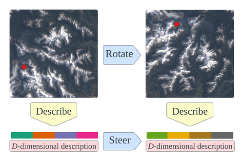
Figure 2: Overview of approach. A steerer (Definition 3.4) is a linear map that transforms the description of a keypoint to the description of the corresponding keypoint in a rotated image. Thus a steerer makes the keypoint descriptor rotation equivariant and we can obtain the descriptions of keypoints in arbitrarily rotated images while only running the descriptor once.

In this paper, we present an approach that maintains distinctiveness for small rotations and allows for rotation invariant matching when we have images with large rotations. We do this while adding only negligible additional runtime, and only run the model a single time. The main idea is to learn a linear transform in description space that corresponds to a rotation of the input image, see Figure 2. We call this linear transform a steerer as it allows us to modify keypoint descriptions as if they were describing rotated images—we can steer the descriptions without having to rerun the descriptor network. Through theoretical arguments and empirical results, we show that approximate steerers can be obtained for existing descriptors. We also investigate jointly optimizing steerers and descriptors and show how this enables nearly exact steering while not sacrificing performance on upright images. By using mathematical group theory, we can describe all possible steerers—they are representations of the rotation group. This enables choosing a fixed steerer and training a descriptor for it, and in turn, to investigate what steerers are the best choice for performance. We believe that our framework should be of interest to both the image matching community and researchers interested in group equivariant neural networks.

Using our framework, we set a new state-of-the-art on the rotation invariant matching benchmarks AIMS [44] (Figure 1) and Roto-360 [27]. At the same time, we are with the same models able to perform on par with or even outperform existing non-invariant methods on upright images on the competitive MegaDepth-1500 benchmark [29, 45].

In summary, our main contributions are as follows.

1. We introduce a new framework of steerers for equivariant keypoint descriptors (Section 3) and theoretically motivate why steerers emerge in practice (Section 4).

2. We develop several settings for investigating steerers (Section 4.1) and ways to apply them for rotation invariant matching (Section 4.2).

3. We conduct a large set of experiments, culminating in state-of-the-art on AIMS and Roto-360 (Section 5).

1.1 Related work

1. A common approach for creating rotation invariance is canonicalization of the local frame [55, 33, 25, 26]. A major downside is that it requires patch-based descriptors [55, 32, 47, 48], as the canonicalization will vary across the image.

2. LF-Net [34] learns $C_{2}$ equivariance through data augmentation. Another line of research uses equivariant convolutional neural networks [13, 53, 51] to produce invariant descriptions [8, 2, 27]. While such approaches can in theory produce exact equivariance, in practice, methods such as SE2-LoFTR [8] are not rotation invariant [8, 44]. It has also been demonstrated that equivariant ConvNets can learn to break equivariance [16] when this is beneficial to the task at hand. In contrast to the case of equivariant ConvNets, our approach works for arbitrary network architectures. This means that we can use pretrained backbones that do not use equivariant layers and that we do not need to specify the group representations acting on the outputs of each layer in the network.

3. A recent line of work [28, 20, 9, 10], investigates to what extent neural networks exhibit equivariance without having been trained or hard-coded to do so. They find that many networks are approximately equivariant. One major limitation is that they only consider networks trained on image classification. We will empirically demonstrate a high level of equivariance in keypoint descriptors that were not explicitly trained to be equivariant and theoretically motivate why this happens.

2 Preliminaries

In this work, we are interested in finding linear mappings between keypoint descriptors where the images may both have been rotated independently. We will in particular consider the group of quarter rotations $C_{4}$ and the group of continuous rotations $\mathrm{SO}(2)$.

Ordinary typeset $g$ will denote an arbitrary group element, boldface $\mathbf{g}$ will always mean the generator of $C_{4}$ for the remainder of the text, so that the elements of $C_{4}$ are $\mathbf{g}$, $\mathbf{g}^{2}$, $\mathbf{g}^{3}$ and the identity element $\mathrm{id}=\mathbf{g}^{4}$. Boldface $\mathbf{i}$ will denote the imaginary unit such that $\mathbf{i}^{2}=-1$. Given matrices $X_{1},X_{2},\ldots,X_{J}$, the notation $\oplus_{b=1}^{J}X_{j}$ will mean the block-diagonal matrix with blocks $X_{1},X_{2},\ldots,X_{J}$.

2.1 Preliminaries on keypoint matching

The underlying task is to take two images of the same scene and detect 2D points that correspond to the same 3D point. A pair of such points that depict the same 3D point is called a correspondence. The approach for finding correspondences that will be explored is a three stage approach:

1. Detection. Detect $N$ keypoint locations in each image.

2. Description. Describe the keypoint locations with descriptors, i.e., feature vectors in $\mathbb{R}^{D}$.

3. Matching. Match the descriptors, typically by using mutual nearest neighbours in cosine distance.

This is a classical setup which includes SIFT [30] but also more recent deep learning based approaches. In particular, we follow the method in DeDoDe [17], where the keypoint detector is first optimized to find good point tracks from SfM reconstructions and the keypoint descriptor is optimized by maximizing the matching likelihood obtained by a frozen keypoint detector as follows. If the $N$ descriptors (each normalized to unit length) in the two images are $y_{1}\in\mathbb{R}^{D\times N}$ and $y_{2}\in\mathbb{R}^{D\times N}$ we first form the $N\times N$ matching matrix $Y=y_{1}^{T}y_{2}$, and obtain a matrix of pairwise likelihoods by using the dual softmax [40, 49, 45]:

$$p(y_{1},y_{2})=\frac{\exp(\iota Y)}{\sum_{\text{columns}}\exp(\iota Y)}\cdot\frac{\exp(\iota Y)}{\sum_{\text{rows}}\exp(\iota Y)}.$$ (1)

Here $\iota=20$ is the inverse temperature. The negative logarithm of the likelihood (1) is minimized for those pairs in the $N\times N$ matrix that correspond to ground truth inliers.

2.2 Preliminaries on group representations

Definition 2.1.

(Group representation) Given a group $G$, a representation of $G$ on $\mathbb{R}^{D}$ is a mapping

$$\rho:G\to\text{GL}(\mathbb{R},D)$$ (2)

that preserves the group multiplication, i.e., $\rho(gg^{\prime})=\rho(g)\rho(g^{\prime})$ for every $g,g^{\prime}\in G$.

Simply stated, $\rho$ maps every element in the group to an invertible $D\times D$ matrix. The point of using representations is that groups such as $C_{4}$ act differently on different quantities as we will illustrate in the following examples.

Example 2.1.

For $\mathbb{R}^{n\times n}$ (a square image grid), $C_{4}$ can be represented by permutations of the pixels in the obvious way so that the image is rotated anticlockwise by multiples of $90\mathrm{°}$. We denote this group representation by $P_{90}$ so that applying $P_{90}^{k}$ rotates the image by $k\cdot$$$ anticlockwise.

Example 2.2.

For $\mathbb{R}^{2}$ (image coordinates), one possible representation of $C_{4}$ is

$$\rho(\mathbf{g}^{k})=R_{90}^{k}=\begin{pmatrix}0&-1\\ 1&0\\ \end{pmatrix}^{k}.$$ (3)

Multiplication by $R^{k}_{90}$ corresponds to rotating image coordinates by $k\cdot$$$ if the center of the image is taken as $(0,0)$.

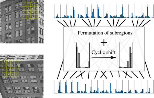
Figure 3: Equivariance of Upright SIFT. Left: A keypoint with its Upright SIFT description in an upright image and a rotated version. The small yellow squares are the subregions where histograms of gradient orientations are computed. Right: The Upright SIFT descriptions unravelled into the 128 bin histograms that constitute them. When we rotate the image, the subregions are permuted and the histogram bins within each subregion is further permuted cyclically. This means that Upright SIFT is rotation equivariant. Here we use the VLFeat convention when illustrating the SIFT histograms [50].

3 Equivariance and steerability

In this section, we will reveal and analyze the close connection between equivariance and steerability. We start by an example in order to introduce the former concept.

Example 3.1.

SIFT descriptions [30] are $128$ dimensional vectors designed to be invariant to rotation, scale and illumination and highly distinctive for leveraging feature matching. For an input image $I\in\mathbb{R}^{n\times n}$ and $N$ keypoints with scale and orientation $x\in\mathbb{R}^{4\times N}$, we get descriptions $y\in\mathbb{R}^{128\times N}$. If $f$ is the SIFT descriptor we write $f(I,x)=y$. The descriptions consist of histograms of image gradients over image patches around the keypoints $x$. The patches are oriented by the keypoint orientations so that the descriptions are invariant to joint rotations of the image and keypoints:

$$f\left(P_{90}^{k}I,(\oplus_{b=1}^{2}R_{90})^{k}x\right)=f(I,x).$$

If we discard the keypoint orientations, i.e., set the angle of each keypoint to $0$, we get the Upright SIFT (UPSIFT) descriptor [7, 1], which is often used for upright images as it is more discriminative than SIFT. When we rotate an image $90\mathrm{°}$, then the gradient histograms, i.e., the UPSIFT descriptions are permuted by a specific permutation $P_{\text{UPSIFT}}$, so if $f$ is the UPSIFT descripor, we have

$$f\left(P_{90}^{k}I,(\oplus_{b=1}^{2}R_{90})^{k}x\right)=P_{\text{UPSIFT}}^{k}f(I,x).$$

We illustrate the permutation $P_{\text{UPSIFT}}$ in Figure 3. UPSIFT is not rotation invariant, but it is rotation equivariant—when we rotate the input, the output changes predictably. Explicitly, the representation is $\rho(\mathbf{g}^{k})=P_{\text{UPSIFT}}^{k}$.

Definition 3.1 (Equivariance).

We say that a function $f:V\to W$ is equivariant with respect to a group $G$ if

$$\rho(g)f(v)=f(\rho_{\text{in}}(g)v),\forall v\in V,g\in G,$$ (4)

for some group representations $\rho_{\text{in}},\rho$.

In this work we will mainly be concerned with equivariance of learned keypoint descriptors of ordinary keypoints (without scale and orientation).

Definition 3.2 (Equivariance of keypoint descriptor).

We say that a keypoint descriptor $f$ is equivariant with respect to a group $G$ transforming the input image by $\rho_{\text{image}}$ and the input keypoint locations by $\rho_{\text{keypoint}}$ if there exists $\rho$ such that

$$\rho(g)f(I,x)=f(\rho_{\text{image}}(g)I,\rho_{\text{keypoint}}(g)x)$$ (5)

for all images, keypoints and group elements. We call the descriptor invariant if $\rho(g)$ is the identity matrix for all $g$, which is a special type of equivariance.

Example 3.2.

A keypoint descriptor $f$ is equivariant under $90\mathrm{°}$ rotations if there exists $\rho$ of $C_{4}$ such that

$$\rho(\mathbf{g}^{k})f(I,x)=f(P_{90}^{k}I,R_{90}^{k}x)$$ (6)

for $k\in\{0,1,2,3\}$, where $P_{90}$ and $R_{90}$ are the representations from Examples 2.1 and 2.2 that rotate images and coordinates in the ordinary manner.

Both SIFT and Upright SIFT are equivariant. For SIFT, $\rho(\mathbf{g}^{k})$ is the identity, so SIFT is invariant. For Upright SIFT, $\rho(\mathbf{g}^{k})$ is $P_{\text{UPSIFT}}^{k}$ as explained in Example 3.1.

One aim of this work is to argue and demonstrate that learned keypoint descriptors, that are trained on upright data, will behave more like Upright SIFT than SIFT, i.e., they will be rotation equivariant but not invariant.

Definition 3.3 (Steerability, adapted from [18] to arbitrary groups)).

A real-valued function $\phi:V\to\mathbb{R}$ is said to be steerable under a representation $\rho_{\text{in}}$ of $G$ on $V$, if there exists a set of functions $\phi_{j}:V\to\mathbb{R}$ and a set of functions $\kappa_{j}:G\to\mathbb{R}$ such that

$$\phi(\rho_{\text{in}}(g)v)=\sum_{j=1}^{D}\kappa_{j}(g)\phi_{j}(v).$$ (7)

Note that an equivariant function $f:V\to\mathbb{R}^{D}$ satisfies in each component $f_{d}$ that $f_{d}(\rho_{\text{in}}(g)v)=\sum_{j=1}^{D}\rho(g)_{dj}f_{j}(v),$ so each component of $f$ is steerable—in the notation of Definition 3.3 $\phi=f_{d},\phi_{j}=f_{j},\kappa_{j}(g)=\rho(g)_{dj}$. This motivates the definition of a steerer.

Definition 3.4 (Steerer).

A steerer for a group $G$ is a representation that makes a function equivariant under $G$. That is, given a function $f:V\to W$, and a representation $\rho_{\text{in}}$ of $G$ on $V$, a steerer is a representation $\rho$ of $G$ on $W$ such that

$$f(\rho_{\text{in}}(g)v)=\rho(g)f(v).$$ (8)

Even if (8) only holds approximately or $\rho$ is only approximately a representation, we will refer to $\rho$ as a steerer.

We will use the verb steer for multiplying a feature/description by a steerer, see Figure 2 for the broad idea.

Example 3.3.

As explained in Example 3.1, $P_{\text{UPSIFT}}$ is a steerer for Upright SIFT under $90\mathrm{°}$ rotations. This has practical consequences. If we want to obtain the Upright SIFT descriptions for an image $I$ and the same image rotated $k\cdot$$$, then we only need to compute the descriptions for the original image and can obtain the rotated ones by simply multiplying the descriptions by $P_{\text{UPSIFT}}^{k}$. That is, we can steer the Upright SIFT descriptions with $P_{\text{UPSIFT}}$.

It is known from representation theory [42] what all possible representations of $C_{4}$ are, and hence what all possible steerers for rotation equivariant descriptors are. As this result will be important for the remainder of the text, we collect it in a theorem. Similar results are also known for other groups e.g. the continuous rotation group $\mathrm{SO}(2)$, which we discuss in the next section.

Theorem 3.1 (Representations of $C_{4}$).

Let $\rho$ be a representation of $C_{4}$ on $\mathbb{R}^{D}$. Then, there exists an invertible matrix $Q$ and $j_{d}\in\{0,1,2,3\}$ such that

$$\rho(\mathbf{g}^{k})=Q^{-1}\mathrm{diag}(\mathbf{i}^{kj_{1}},\mathbf{i}^{kj_{2}},\ldots,\mathbf{i}^{kj_{D}})Q.$$ (9)

The diagonal in (9) contains the eigenvalues of $\rho(\mathbf{g}^{k})$.

Example 3.4.

The Upright SIFT steerer $P_{\text{UPSIFT}}$ is diagonalizable with an equal amount of each eigenvalue $\pm 1$, $\pm\mathbf{i}$.

As we take $\rho(\mathbf{g})$ to be real valued, the complex eigenvalues must appear in conjugate pairs. It is then possible to change basis so that each pair $\mathbf{i},-\mathbf{i}$ on the diagonal in (9) is replaced by a block $\left(\begin{smallmatrix}0&-1\\ 1&0\end{smallmatrix}\right)$. In this way, $\rho(\mathbf{g})$ can always be block-diagonalized: $\rho(\mathbf{g})=Q^{-1}BQ$ where $Q$ and $B$ are real valued and $B$ is block-diagonal with blocks of sizes 1 and 2.

3.1 Representation theory of $\mathrm{SO}(2)$

$\mathrm{SO}(2)$ is a one parameter Lie group, meaning that it is a continuous group with one degree of freedom $\alpha$—the angle of rotation. A $D$-dimensional representation of $\mathrm{SO}(2)$ is a map $\varsigma:[0,2\pi)\to\mathrm{GL}(\mathbb{R},D)$ such that addition modulo $2\pi$ on the input is encoded as matrix multiplication on the output—we will consistently use $\varsigma$ for $\mathrm{SO}(2)$ representations to separate them from $C_{4}$ representations $\rho$ ($\rho$ will also be used for representations of general groups). The most familiar is the two-dimensional representation $\varsigma(\alpha)=\left(\begin{smallmatrix}\cos(\alpha)&-\sin(\alpha)\\ \sin(\alpha)&\cos(\alpha)\end{smallmatrix}\right)$ which rotates 2D coordinates. Similar to the $C_{4}$ case in Theorem 3.1, we can write down a general representation for $\mathrm{SO}(2)$ as follows [52].

Theorem 3.2 (Representations of $\mathrm{SO}(2)$).

Let $\varsigma$ be a representation of $\mathrm{SO}(2)$ on $\mathbb{R}^{D}$. Then there exists an invertible $Q$ and $j_{d}\in\mathbb{Z}$ such that

$$\varsigma(\alpha)=Q^{-1}\mathrm{diag}\left(\mathrm{e}^{\mathbf{i}j_{1}\alpha},\mathrm{e}^{\mathbf{i}j_{2}\alpha},\ldots,\mathrm{e}^{\mathbf{i}j_{D}\alpha}\right)Q.$$ (10)

The $j_{d}$’s are the frequencies of the eigenspaces of $\varsigma$. Complex eigenvalues appear in conjugate pairs so (10) can be rewritten as a block diagonal decomposition $\varsigma(\alpha)=Q^{-1}BQ$ where $Q$ and $B$ are real valued and $B$ is block-diagonal with minimal blocks. The admissible blocks ($=$ real valued irreducible representations) in $B$ are then the $1\times 1$ block $\begin{pmatrix}1\end{pmatrix}$ and the $2\times 2$ blocks

$$\begin{pmatrix}\cos(j\alpha)&-\sin(j\alpha)\\ \sin(j\alpha)&\cos(j\alpha)\end{pmatrix}\quad\text{for $j\in\mathbb{Z}\setminus\{0\}$.}$$ (11)

We can write $\varsigma(\alpha)=\operatorname{expm}\left(\alpha Q^{-1}\mathrm{diag}(\mathbf{i}j_{1},\ldots,\mathbf{i}j_{D})Q\right)$ where $\operatorname{expm}$ is the matrix exponential. The quantity $\mathrm{d}\varsigma=Q^{-1}\mathrm{diag}(\mathbf{i}j_{1},\ldots,\mathbf{i}j_{D})Q$ is called a Lie algebra representation of $\mathrm{SO}(2)$, here in its most general form. When training a steerer for $\mathrm{SO}(2)$ it is practical to train a $D\times D$ matrix $\mathrm{d}\varsigma$ and steer using $\varsigma(\alpha)=\operatorname{expm}(\alpha\mathrm{d}\varsigma)$.

3.2 Disentangling description space

When we have a steerer, we get a description space on which rotations act—up to a change of basis—by a block-diagonal matrix $\oplus_{j=1}^{J}B_{j}$. The description space can then be thought of as being disentangled into different subspaces where rotations act in different ways $B_{j}$ [12]. We detail what this means for keypoint descriptors in Appendix A.

4 Descriptors and steerers

Our key observation and assumption in this work is that learned descriptors, while not invariant, are approximately equivariant so that they have a steerer. Or, as a weaker assumption, that they can be trained to be equivariant. It may seem that this is a strong assumption. However, a seemingly less strong assumption turns out to be equivalent.

Theorem 4.1.

[Shakerinava et al. [43], Gupta et al. [21], adapted] Assume that we have a function $f:V\to\mathbb{S}^{D-1}$ and a group $G$ with representation $\rho_{\text{in}}$ on $V$ such that, for all $v\in V$ and $g\in G$

$$\langle f(\rho_{\text{in}}(g)v),f(\rho_{\text{in}}(g)v^{\prime})\rangle=\langle f(v),f(v^{\prime})\rangle.$$ (12)

Then there exists an orthogonal representation $\rho(g)$, such that $f$ is equivariant w.r.t. $G$ with representations $\rho_{\text{in}}$ and $\rho$.

We provide a proof in Appendix A. Since we match normalized keypoint descriptions by their cosine similarity, Theorem 4.1 is highly applicable to the image matching problem. If a keypoint descriptor $f$ is perfectly consistent in the matching scores when simultaneously rotating the images, then the scalar products in (12) will be equal so that the theorem tells us that $f$ has a steerer $\rho$. Furthermore, we can expect many local image features to appear in all orientations even over a dataset of upright images, thus encouraging (12) to hold for $f$ trained on large datasets.

4.1 Three settings for investigating steerers

As $C_{4}$ is cyclic, all its representations are defined by $\rho(\mathbf{g})$, where $\mathbf{g}$ is the generator. To find a steerer for a keypoint descriptor under $C_{4}$ hence comes down to finding a single matrix $\rho(\mathbf{g})$ that represents rotations by $90\mathrm{°}$ in the description space. Similarly, for $\mathrm{SO}(2)$ we find the single matrix $\mathrm{d}\varsigma$ that defines the representation $\varsigma$.

We will in the following consider three settings. In each case we will optimize $\rho(\mathbf{g})$ and/or $f$ over the MegaDepth training set [29] with rotation augmentation and maximize

$$p\left(f(P_{90}^{k_{1}}I_{1},R_{90}^{k_{1}}x_{1}),\rho(\mathbf{g})^{k}f(P_{90}^{k_{2}}I_{2},R_{90}^{k_{2}}x_{2})\right)$$ (13)

where $p$ is the matching probability (1). The number of rotations $k_{1}$ and $k_{2}$ for each image are sampled independently during training and $k=k_{1}-k_{2}\mod{4}$ is the number of rotations that aligns image $I_{2}$ to image $I_{1}$. Thus, $\rho(\mathbf{g})^{k}$ aligns the relative rotation between descriptions in $I_{2}$ and $I_{1}$. We optimize continuous steerers $\varsigma$ analogously to (13).

1. If a descriptor works equally well for upright images as well as images rotated the same amount from upright, then according to Theorem 4.1 we should expect that there exists a steerer $\rho(\mathbf{g})$ such that (6) holds. To find $\rho(\mathbf{g})$ we optimize it as a single $D\times D$ linear layer by maximizing (13).

2. The aim is to find a steerer that is as good as possible for the given data. We will see in the experiments, by looking at the evolution of the eigenvalues of $\rho(\mathbf{g})$ during training, that this joint optimization has many local optima and is highly dependent on the initialization of $\rho(\mathbf{g})$. However, looking at the eigenvalues of $\rho(\mathbf{g})$ does give us knowledge about which dimensions of the descriptor are most important as will be explained in Section 5.5.

3. To get the most precise control over the rotation behaviour of a descriptor, we can fix the steerer and optimize only the descriptor. This enables us to investigate how much influence the choice of steerer has on the descriptor. For instance, choosing the steerer to be the identity leads to a rotation invariant descriptor, but we will see in the experiments that this choice leads to suboptimal performance on upright images compared to other steerers.

Table 1: Evaluation on Roto-360 [27]. We report the percentage of correct matches at certain pixel thresholds. For DeDoDe detectors we report results with $5,000$ keypoints. See Section 5.1 for shorthand explanations for our models.

Detector	Descriptor	3px	5px	10px
SIFT [30]	SIFT [30]	78	78	79
ORB [41]	ORB [41]	79	85	87
SuperPoint [15]	RELF, single [27]	90	91	93
SuperPoint [15]	RELF, multiple [27]	92	93	94
SuperPoint [15]	C4-B (ours)	82	82	83
SuperPoint [15]	SO2-Spread-B (ours)	96	97	97
DeDoDe [17]	C4-B (ours)	82	84	86
DeDoDe [17]	SO2-Spread-B (ours)	95	97	98

4.2 Matching with equivariant descriptions

In this section we present several approaches to rotation invariant matching using equivariant descriptors. Throughout, we will denote the $D$-dimensional descriptions of $N$ keypoints in two images $I_{1},I_{2}$ by $y_{1},y_{2}\in\mathbb{R}^{D\times N}$ and will assume that we know the $C_{4}$-steerer $\rho(\mathbf{g})$ that rotates descriptions $90\mathrm{°}$ or the $\mathrm{SO}(2)$-steerer $\varsigma(\alpha)$ through the Lie algebra generator $\mathrm{d}\varsigma$. For matching we follow DeDoDe [17], as described in Section 2.1. The base similarity used is the cosine similarity, so we compute $y_{1}^{T}y_{2}$ for normalized descriptions to get an $N\times N$ matrix of pairwise scores on which dual softmax (1) is applied. Mutual most similar descriptions are chosen, with similarity above $0.1$, as matches.

1. The first way of obtaining invariant matches is to match $y_{1}$ with $\rho(\mathbf{g})^{k}y_{2}$ for $k=0,1,2,3$, and keep the matches from the number of rotations $k$ that has most matches. This is similar to the strategy of matching the image $I_{1}$ with four different rotations of $I_{2}$, but alleviates the need for rerunning the descriptor network for each rotation. This works if the entire image is globally rotated, not if parts are rotated independently.

2. A computationally cheaper version is to select the matching matrix not as $y_{1}^{T}y_{2}$ but as $\max_{k}y_{1}^{T}\rho(\mathbf{g})^{k}y_{2}$, where the $\max$ is elementwise over the matrix.

3. To apply the above matching strategies to $\mathrm{SO}(2)$-steerers $\varsigma(\alpha)$, we discretize $\varsigma(\alpha)=\operatorname{expm}(\alpha\mathrm{d}\varsigma)$. A $C_{\ell}$-steerer is obtained through $\operatorname{expm}\left(\frac{k\pi}{\ell}\mathrm{d}\varsigma\right)$. We will use $C_{8}$-steerers in the experiments.

4. If all eigenvalues of $\rho(\mathbf{g})$ are $\pm\mathbf{i}$, then the steerer can be block-diagonalized with only the block $\left(\begin{smallmatrix}0&-1\\ 1&0\end{smallmatrix}\right)$. The descriptions consist of $D/2$ two-dimensional quantities that all rotate with the same frequency as the image. We will refer to them as frequency 1 descriptions and view them reshaped as $y\in\mathbb{R}^{2\times(D/2)\times N}$. A 2D rotation matrix acts on these descriptions from the left when the image rotates and we can find the optimal rotation matrix $R_{m,n}$ that aligns each pair $y_{1,m},y_{2,n}\in\mathbb{R}^{2\times(D/2)}$ by solving the Procrustes problem via an SVD. The matching matrix is obtained by computing $\langle R_{m,n}y_{1,m},y_{2,n}\rangle$ for each pair. $R_{m,n}$ gives the relative rotation between each pair of keypoints, which can be useful e.g. for minimal relative pose solvers [6, 4] or for outlier filtering [11]. We leave exploring this per-correspondence geometry to future work.

Table 2: Evaluation on AIMS [44]. We report the average precision (AP) in percent on different splits of AIMS: “North Up” (N. Up) contains images with small rotations, “All Others” (A. O.) contains images with larger rotations and “All” contains all images. We use the DeDoDe-SO2 detector and $10,000$ keypoints throughout. See Section 5.1 for shorthand explanations for our models.

Detector	Descriptor	N. Up	A. O.	All
–	SE2-LoFTR [8]	58	51	52
DeDoDe [17]	C4-B (ours)	52	51	51
DeDoDe [17]	SO2-Spread-B (ours)	60	57	58
DeDoDe [17]	SO2-Freq1-B (ours)	64	59	60

Table 3: Evaluation on MegaDepth [29, 45]. The first section shows Setting A where we only optimize the steerer, the second section shows Setting B where we jointly optimize the descriptor and steerer and the third section shows the Setting C where we predefine the steerer and optimize only the descriptor. For MegaDepth-1500 we always use dual softmax matcher to evaluate the descriptors on upright images. We use $20,000$ keypoints throughout. The best values for B- and G-models are highlighed in each column. See Section 5.1 for shorthand explanations for our models. A larger version of this table with more methods is available in Appendix B.

Detector	Descriptor		AUC @ MegaDepth-1500			MegaDepth-C4			MegaDepth-SO2
DeDoDe	DeDoDe	Matching strategy	AUC $@$  $5^{\circ}$	$10^{\circ}$	$20^{\circ}$	$5^{\circ}$	$10^{\circ}$	$20^{\circ}$	$5^{\circ}$	$10^{\circ}$	$20^{\circ}$
Original	B	Dual softmax	49	65	77	12	17	20	12	16	20
Original	B	Max matches C4-steered				43	60	73	30	44	56
SO2	B	Max matches C8-steered	50	66	78	40	57	70	34	51	65
Original	G	Dual softmax	52	69	81	13	17	21	16	22	28
Original	G	Max matches C4-steered				31	45	57	26	39	50
C4	C4-B	Max matches C4-steered	51	67	79	50	67	79	39	55	68
SO2	SO2-B	Max matches C8-steered	47	63	76	47	63	76	44	61	74
SO2	SO2-Spread-B	Max matches C8-steered	50	66	79	49	66	78	46	63	76
SO2	SO2-Spread-B	Max similarity C8-steered	49	66	78	47	64	77	43	61	74
C4	C4-Inv-B	Dual softmax	48	64	76	47	63	76	39	55	69
C4	C4-Perm-B	Max matches C4-steered	50	67	79	50	66	79	39	54	67
SO2	SO2-Inv-B	Dual softmax	46	62	75	45	61	74	43	60	73
SO2	SO2-Freq1-B	Max matches C8-steered	47	64	77	47	64	76	45	62	75
SO2	SO2-Freq1-B	Procrustes	47	64	76	46	62	75	45	61	74
C4	C4-Perm-G	Max matches C4-steered	52	69	81	53	69	82	44	61	74

5 Experiments

We train and evaluate a variety of matchers and steerers. We make code and model weights publicly available at github.com/georg-bn/rotation-steerers. Further experiments are presented in Appendix B followed by more details in Appendix C.

We start by reporting results on two public benchmarks for rotation invariant image matching. Then, we will present ablation results for the MegaDepth benchmark, both for the standard version with upright images and a version where we have rotated the input images.

5.1 Models considered

Our base models are the DeDoDe detector and the DeDoDe-B and DeDoDe-G descriptors introduced in [17]. These are both $D=256$ dimensional descriptors. The focus will be on the smaller model DeDoDe-B as this gives us the chance to do large scale ablations. We train all models on MegaDepth [29]. To obtain rotation invariant detections, we retrain one version of the DeDoDe-detector each with data augmentation over $C_{4}$ and $\mathrm{SO}(2)$, denoted DeDoDe-C4 and DeDoDe-SO2.

For Setting B (Section 4.1), we will see that the initialization of the steerer matters. Similarly for Setting C, we can fix the steerer with different eigenvalue structures. Here we introduce shorthand used in the result tables. We will refer to the case of all eigenvalues 1 as Inv for invariant. This case corresponds to the ordinary notion of data augmentation, where the descriptions for rotated images should be the same as for non-rotated images. The case when all eigenvalues are $\pm\mathbf{i}$ is denoted Freq1 for frequency 1 as explained in Section $\mathbf{SO(2)}$-steerers. . For $C_{4}$-steerers, the case with an equal distribution of all eigenvalues $\pm 1,\pm\mathbf{i}$ will be denoted Perm, as this is the eigenvalue signature of a cyclic permutation of order 4. For $\mathrm{SO}(2)$-steerers, the case with an equal distribution of eigenvalues $0,\pm\mathbf{i},\pm 2\mathbf{i},\ldots\pm 6\mathbf{i}$ will be denoted Spread (the cutoff $6$ was arbitrarily chosen). The Perm and Spread steerers correspond to a broad range of frequencies in the description space. When no of the above labels (Inv, Freq1, Perm or Spread) is attached to a descriptor and steerer trained jointly in Setting B, then we initialize the steerer with values uniformly in $(-D^{-1/2},D^{-1/2})$, the eigenvalues are then approximately uniformly distributed in the disk with radius $3^{-1/2}$ [46] and move towards the admissible eigenvalues for steerers during training, as will be seen in visualizations in Section 5.5. When a descriptor is trained with $k\cdot$$$ rotations, we append C4 to its name and when it is trained with continuous augmentations we append SO2 to its name.

5.2 Roto-360

We evaluate on the Roto-360 benchmark Lee et al. [27], which consists of ten image pairs from HPatches [3] where the second image in each image pair is rotated by all multiplies of $10\mathrm{°}$ to obtain 360 image pairs in total. We report the average precision of the obtained matches and compare to the current state-of-the-art RELF [27]. The results are shown in Table 1. We see that we outperform RELF when using methods trained for continuous rotations. Our matching runs around three times faster than RELF on Roto-360.

5.3 AIMS

The Astronaut Image Matching Subset (AIMS) [44] consists of images taken by astronauts from the ISS. Each astronaut image is paired with satellite images corresponding to locations that could be seen from the ISS at the point in time when the astronaut image was taken. The task consists in finding the pairs of astronaut images and satellite images that show the same locations on Earth. Using an image matcher this can be done by setting a threshold for number of inlier matches between the images after homography estimation with RANSAC and counting image pairs with number of matches above this threshold as positive pairs.

The relative rotations of the astronaut and satellite images are unknown, making the task suitable for rotation invariant matchers. Indeed, in [44] the best performing method is the rotation invariant SE2-LoFTR [8] which we compare to. The AIMS can be split into “North Up” astronaut images, consisting of images with small rotations (between $0\mathrm{°}$ and $90\mathrm{°}$) and “All Others”, consisting of images with large rotations. This split further enables the evaluation of rotation invariant matchers. We report the average precision over the whole dataset, as opposed to in [44] where the score is computed over maximum 100 true negatives per astronaut image. Results are shown in Table 2. Further, we plot precision-recall curves in Appendix B. We outperform SE2-LoFTR in general and in particular on the heavily rotated images in “All Others”.

5.4 MegaDepth-1500

We evaluate on a held out part of MegaDepth (MegaDepth-1500 [45]). Here the task is to take two input images and output the relative pose between the respective cameras. The keypoint matches produced by our pipeline are processed in a RANSAC loop following the standard protocol introduced in [45]. The performance is measured by the AUC of the pose error. Additionally we create two versions of MegaDepth with rotated images to evaluate the rotational robustness of our models. For MegaDepth-C4, the second image in every image pair is rotated $(i\mod 4)\cdot$$$ where $i$ is the index of the image pair. We visualize a pair in MegaDepth-C4 in Appendix B, illustrating the improvement from DeDoDe-B to DeDoDe-B with a steerer optimized in Setting A. For MegaDepth-SO2, the second image in every image pair is instead rotated $(i\mod 36)\cdot$$$, thus requiring robustness under continuous rotations.

The results are presented in Table 3 and for more methods, see Appendix B. We summarize the main takeaways:

1. It is possible to find steerers for the original DeDoDe models (e.g. the second row of the table), even though they were not trained with any rotation augmentation.

2. The trained $C_{4}$ steerers perform very well as their scores on MegaDepth-1500 and MegaDepth-C4 are the same.

3. Training DeDoDe-B jointly with a $C_{4}$ steerer (C4-B) or with a fixed steerer (C4-Perm-B) improves results on upright images—this can be attributed to the fact that training with a steerer enables using rotation augmentation.

4. The right equivariance for the task at hand is crucial—$\mathrm{SO}(2)$-steerers outperform others on MegaDepth-SO2.

5. The eigenvalue distribution of the steerer is important—invariant models are worse than others and SO2-B and SO2-Freq1-B are worse than SO2-Spread-B.

6. DeDoDe-G can be made equivariant (C4-Perm-G), even though it has a frozen DINOv2 [35] ViT backbone.

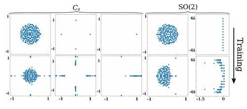
Figure 4: Training evolution of eigenvalue distributions of steerers. We plot the eigenvalue distribution of $C_{4}$-steerers $\rho(\mathbf{g})$ (first three columns) and Lie algebra generators $\mathrm{d}\varsigma$ for $\mathrm{SO}(2)$-steerers (last two columns) in the complex plane, with different initializations when trained jointly with a descriptor. The top row depicts the eigenvalues at the start of training and the bottom row at the end of training. There are $D=256$ eigenvalues in every plot—many congregate at the “admissible” eigenvalues as described in Section 3—but some don’t, see the discussion in Section 5.5. These visualizations highlight the initialization sensitivity of the steerer. We show gif movies of the training evolution at github.com/georg-bn/rotation-steerers.

5.5 Training dynamics of steerer eigenvalues

When training a steerer and descriptor jointly (Setting B), we can hope that the optimization leads to a good eigenvalue structure for the steerer. The purpose of this section is to demonstrate that this is not necessarily the case, since the optimization is highly biased towards the initialization of the steerer in all our experiments. We plot the evolution of the eigenvalues of the steerer over the training epochs in Figure 4. For $C_{4}$-steerers we plot the eigenvalues of $\rho(\mathbf{g})$ itself, while for $\mathrm{SO}(2)$-steerers we plot the eigenvalues $\lambda_{d}$ of the Lie algebra generator $\mathrm{d}\varsigma$, so that the eigenvalues of the steerer $\varsigma(\alpha)$ are $\mathrm{e}^{\alpha\lambda_{d}}$. It is clear from Figure 4 that the initialization of the steerer influences the final distribution of eigenvalues a lot and we saw in Table 3 that the eigenvalue distribution of the steerer matters for performance. Thus we think it is an important direction for future work how to get around this initialization sensitivity. The choice of eigenvalue structure is related to the problem of specifying which group representations to use in the layers of equivariant neural networks in general.

As a side effect of plotting the eigenvalues, we find that some of the steerers eigenvalues have much lower absolute value than others. The steerer is applied to descriptions before they are normalized, so the absolute value of the maximum eigenvalue is unimportant, but the relative size of the eigenvalues tells us something about feature importance. Eigenvectors with small eigenvalues can not be to important for matching, since they will be relatively downscaled when applying the steerer in the optimization of (13). Indeed, small eigenvalues seem to correspond to unimportant dimensions of the descriptor—we maintain matching performance when projecting the descriptions to the span of the eigenvectors with large eigenvalues. This is likely related to methods such as PCA for dimensionality reduction, which has successfully been used for classical keypoint descriptors [23].

6 Conclusion

We developed a new framework for rotation equivariant keypoint descriptors using steerers—linear maps that encode image rotations in description space. By outlining the general theory of steerers using representation theory we were able to design a large set of experiments with steerers in three settings: (A) optimizing a steerer for a fixed descriptor, (B) optimizing a steerer and a descriptor jointly and (C) optimizing a descriptor for a fixed steerer. Our best models obtained new state-of-the-art results on the rotation invariant matching benchmarks Roto-360 and AIMS.

Supplementary Material

Appendix A Supplementary theory

We provide further theoretical discussions that did not have room in the main text. First, Section A.1 contains a discussion of what having representations of $C_{4}$ or $\mathrm{SO}(2)$ on description space means. Section A.2 contains a proof of Theorem 4.1 and Section A.3 presents matching strategies that are considered in the extra ablations of Section B but were omitted from the main paper due to space limitations.

A.1 Disentangling description space

As explained following Theorem 3.1, any representation of $C_{4}$ or $\mathrm{SO}(2)$ can be block-diagonalized over the real numbers into blocks of size $1$ and $2$, called irreducible representations (irreps). We can think of these irreps as disentangling descriptions space [12], i.e. each eigenspace of the steerer is acted on by rotations in a specific way according to the respective irrep. The aim of this section is to explain the relevance of the different irreps to keypoint descriptors. For $C_{4}$, we have the following.

• $1\times 1$ irreps $\begin{pmatrix}1\end{pmatrix}$ act by doing nothing. Hence, the corresponding dimensions in description space are invariant under rotations. For $C_{4}$, image features described by these dimensions could be for instance crosses or blobs.

• $1\times 1$ irreps $\begin{pmatrix}-1\end{pmatrix}$ correspond to dimensions that are invariant under $180\mathrm{°}$ rotations, but not $90\mathrm{°}$ rotations. Examples of such image features could be lines.

• $2\times 2$ irreps $\begin{pmatrix}0&-1\\ 1&0\end{pmatrix}$ correspond to pairs of dimensions that are not invariant under any rotation. Many image features should be of this type, e.g. corners.

For $\mathrm{SO}(2)$ we get the same $\begin{pmatrix}1\end{pmatrix}$ irrep, which in this case represents features invariant under all rotations such as blobs, and the $2\times 2$ irreps in (11) which represent features rotating with $j$ times the frequency of the image. E.g. lines rotate with frequency $j=2$ since when we rotate the image by $180\mathrm{°}$, the line is back to its original orientation.

It is however not the case that the description for a keypoint will lie solely in the dimensions of a single irrep, the description will be a linear combination of quantities that transform according to the different irreps. One can then view the descriptions as a form of non-linear Fourier decomposition of the image features as has been discussed in the literature for general image features, we provide a short discussion in Appendix A.

Example A.1.

In Upright SIFT, the decomposition of the $128$ description dimensions is equally split between the irreps, i.e., there are $32$ invariant dimensions, $32$ dimensions that are invariant under $180\mathrm{°}$ degree rotations and $64$ dimensions which are not invariant under any rotation.

The connections to Fourier analysis of having a group representation acting on the latent space of a model were discussed for linear models in [12] concurrently to this work for neural networks in [24]. We sketch the main idea here to give the reader some intuition. If we have a signal $h$ on $\mathbb{R}^{n}$ and want to know how it transforms under cyclic permutations of the $n$ coordinates, we can take the Discrete Fourier Transform (DFT). Each coordinate $h_{j}$ can be written as a linear combination of Fourier basis functions: $h_{j}=\sum_{k=0}^{n-1}\hat{h}_{k}\exp(2\pi\mathbf{i}jk/n)$ and the DFT is simply the vector $\hat{h}$. When we cyclically permute $h$ by $J$ steps, it corresponds to multiplying each component $\hat{h}_{k}$ by $\exp(2\pi\mathbf{i}Jk/n)$. Thus the cyclic permutation on $h$ acts like a diagonal matrix on the DFT $\hat{h}$. The DFT is a linear transform of the signal $h$. In our setting, the signal consists of images and keypoints, that are transformed by a neural network $f$ to description space. As described in Theorem 3.1, rotations act by a diagonal matrix in description space (up to a change of basis $Q$). In the terminology of [24], we can think of the neural network $f$ as doing a Neural Fourier Transform of the input.

Having group representations act on latent spaces in neural networks has been considered in for instance [54, 14, 31]. In all of these works the specific representation is fixed before training the network, similar to our Setting C. As far as we know, choosing the representation optimally remains an open question—the experiments in this paper showed that this is an important question. [43] and [21] considered using (12) as a loss term to obtain orthogonal representations on the latent space. This approach is promising also for keypoint descriptors, in particular for encoding transformations more complicated than rotations in description space since the approach does not require knowledge of the representation theory of the transformation group in question.

A.2 Proof of Theorem 4.1

Here we give a proof of Theorem 4.1. See 4.1

Proof.

Note that if $f(v)=f(v^{\prime})$, then by (12), $f(\rho_{\text{in}}(g)v)=f(\rho_{\text{in}}(g)v^{\prime})$. This means that we for each $g\in G$ can define a map $\tilde{\varphi}_{g}:f(V)\to f(V)$ by

$$\tilde{\varphi}_{g}(w)=f(\rho_{\text{in}}(g)f^{-1}(w)),$$ (14)

where $f^{-1}(w)$ is any element that $f$ maps to $w$. We next extend $\tilde{\varphi}_{g}$ to a map $\varphi_{g}:\mathbb{S}^{D-1}\to\mathbb{S}^{D-1}$. Start by writing any element $w\in\mathbb{S}^{D-1}$ as

$$w=w_{\bot}+\sum_{i=1}^{n}a_{i}w_{i},$$ (15)

where $a_{i}\in\mathbb{R}$, the $w_{i}$’s are of the form $f(v_{i})$ for some $v_{i}\in V$ and form a basis of $\mathrm{span}(f(V))$ and $w_{\bot}$ is orthogonal to $\mathrm{span}(f(V))$. Define

$$\varphi_{g}(w)=w_{\bot}+\sum_{i=1}^{n}a_{i}\tilde{\varphi}_{g}(w_{i}).$$ (16)

We can now use (12) to show that $\varphi_{g}$ is an isometry of the sphere $\mathbb{S}^{D-1}$, i.e. an orthogonal transformation:

$$\langle\varphi_{g}(w),\varphi_{g}(w^{\prime})\rangle =\langle w_{\bot},w^{\prime}_{\bot}\rangle$$ (17)

$$\phantom{=}+\sum_{i=1}^{n}\sum_{j=1}^{n}a_{i}a^{\prime}_{j}\langle\tilde{\varphi}_{g}(w_{i}),\tilde{\varphi}_{g}(w_{j})\rangle$$ (18)

$$\stackrel{{\scriptstyle\begin{subarray}{c}\eqref{eq:gupta}\\ \eqref{eq:tildephi}\end{subarray}}}{{=}}\langle w_{\bot},w^{\prime}_{\bot}\rangle+\sum_{i=1}^{n}\sum_{j=1}^{n}a_{i}a^{\prime}_{j}\langle w_{i},w_{j}\rangle$$ (19)

$$=\langle w,w^{\prime}\rangle.$$ (20)

As it is an orthogonal transformation, we can write $\varphi_{g}$ as being a matrix acting on vectors in $\mathbb{S}^{D-1}$ by matrix multiplication. Finally, we need to show that $\rho(g)=\varphi_{g}$ defines a representation of $G$, i.e. that $\varphi_{g}\varphi_{g^{\prime}}=\varphi_{gg^{\prime}}$ for all $g,g^{\prime}\in G$. We begin by showing that $\varphi_{g}$ and $\tilde{\varphi}_{g}$ are equal on $f(V)$, which now follows from linearity of $\varphi_{g}$ as follows. Take a general $w\in f(V)$, and again write $w=\sum_{i=1}^{n}a_{i}w_{i}$, then

$$\langle\varphi_{g}(w),\tilde{\varphi}_{g}(w)\rangle =\left\langle\varphi_{g}\left(\sum_{i=1}^{n}a_{i}w_{i}\right),\tilde{\varphi}_{g}(w)\right\rangle$$ (21)

$$=\sum_{i=1}^{n}a_{i}\langle\varphi_{g}(w_{i}),\tilde{\varphi}_{g}(w)\rangle$$ (22)

$$\stackrel{{\scriptstyle\eqref{eq:defphi}}}{{=}}\sum_{i=1}^{n}a_{i}\langle\tilde{\varphi}_{g}(w_{i}),\tilde{\varphi}_{g}(w)\rangle$$ (23)

$$\stackrel{{\scriptstyle\eqref{eq:gupta}}}{{=}}\sum_{i=1}^{n}a_{i}\langle w_{i},w\rangle$$ (24)

$$=\langle w,w\rangle$$ (25)

$$=1$$ (26)

so that $\varphi_{g}(w)=\tilde{\varphi}_{g}(w)$. For the $w_{i}$’s from before we thus have

$$\varphi_{gg^{\prime}}w_{i} =\tilde{\varphi}_{gg^{\prime}}(w_{i})$$ (27)

$$=f(\rho_{\text{in}}(gg^{\prime})v_{i})$$ (28)

$$=f(\rho_{\text{in}}(g)\rho_{\text{in}}(g^{\prime})v_{i})$$ (29)

$$=\tilde{\varphi}_{g}(f(\rho_{\text{in}}(g^{\prime})v_{i}))$$ (30)

$$=\tilde{\varphi}_{g}(\tilde{\varphi}_{g^{\prime}}(f(v_{i})))$$ (31)

$$=\tilde{\varphi}_{g}(\tilde{\varphi}_{g^{\prime}}(w_{i}))$$ (32)

$$=\tilde{\varphi}_{g}(\varphi_{g^{\prime}}(w_{i}))$$ (33)

$$=\varphi_{g}\varphi_{g^{\prime}}w_{i}.$$ (34)

Further, for any $w_{\bot}$ orthogonal to $\mathrm{span}(f(V))$ we have

$$\varphi_{gg^{\prime}}w_{\bot}=w_{\bot}=\varphi_{g}\varphi_{g^{\prime}}w_{\bot}.$$ (35)

Thus by linearity $\varphi_{gg^{\prime}}=\varphi_{g}\varphi_{g^{\prime}}$. ∎

A.3 More matching strategies

We discuss more potential matching strategies. Their performance is shown in the large ablation Table 5.

1. Given a steerer $\rho(\mathbf{g})$, we can project to the rotation invariant subspace of the descriptions by taking $\sum_{k=0}^{3}\rho(\mathbf{g})^{k}y/4$ as descriptions instead of $y$. It is also possible to do this projection by decomposing $\rho(\mathbf{g})$ using (9). However, we will see that these invariant descriptions do not perform very well (but still better than just using $y$). This is likely due to the fact that the invariant subspace is typically only one fourth of the descriptor space.

2. We can estimate the best relative rotation between two images by using the max matches matching strategy on only a subset of the keypoints in each image. The obtained rotation is then used to steer the descriptions of all keypoints. This subset matcher strategy gives lower runtime while not sacrificing performance much. In our experiments we use $1,000$ keypoints.

3. For frequency 1 descriptors, as a way to make the Procrustes matcher less computationally expensive, we propose instead of aligning each description pair optimally, to align every description to a prototype description $\tilde{y}\in\mathbb{R}^{2\times(D/2)}$. Thus, we solve the Procrustes matcher once per description in each image, to obtain $2N$ rotation matrices $R_{1,m}$ and $R_{2,n}$, and form the matching matrix with elements $\langle\mathtt{flatten}(R_{1,m}y_{1,m}),\mathtt{flatten}(R_{2,n}y_{2,n})\rangle$. $\tilde{y}$ can be obtained by optimizing it over a subset of the training set for a fixed frequency 1 descriptor. This strategy is similar to the group alignment proposed in RELF [27], however there the alignment is done using a single feature in a permutation representation of $C_{16}$, whereas we look at the entire $D$-dimensional description. We could similarly to RELF use only certain dimensions of the descriptions for alignment and add a loss for this during training, however we leave this and a careful examination of optimal alignment strategies to future work.

Appendix B More experiments

In this section we present ablations that did not have room in the main paper. A large table of results is provided as Table 5. Further, we present an experiment in support of using Theorem 4.1 to motivate the existence of steerers in Section B.1 and a comparison to test time rotation augmentation in terms of performance and runtime in Section B.2

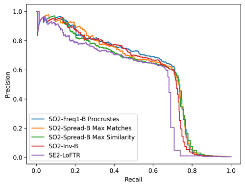
Figure 5: Precision-recall on AIMS. We plot precision-recall curves over the complete AIMS.

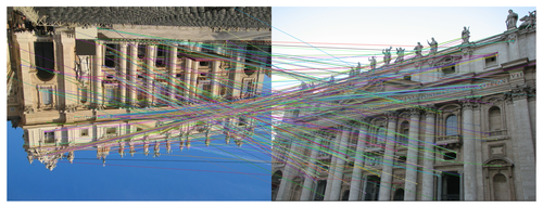
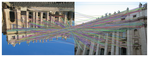
Figure 6: Steering DeDoDe descriptions under half turn rotations. We replicate [17, Figure 7] but with a steerer. In the left image pair we match the ordinary DeDoDe-descriptions. In the right image pair we instead modify the descriptions of the keypoints in the right image by multiplying them by a steering matrix $\rho(\mathbf{g})^{2}$. This corresponds to setting A, where we for a fixed desciptor have optimized a steerer.

Figure 6 shows an example of the improvement obtained by using a steerer for large rotations. Figure 5 shows the recall-precision curves for the experiments on AIMS from Section 5.3.

B.1 Equal rotation augmentation

We explained the spontaneous equivariance of DeDoDe-B by referring to Theorem 4.1 and saying that descriptors will be equivariant if the performance is equivalent for matching images $I_{1}$ and $I_{2}$ as matching jointly rotated images $P_{90}^{k}I_{1}$ and $P_{90}^{k}I_{2}$. To test this explanation we can look at whether the equivariance of a keypoint descriptor relates to how good it is at matching jointly rotated images.

We experiment with four different descriptors, DeDoDe-B, DeDoDe-G, DISK [49] and a retrained DeDoDe-B with data augmentation where both images are rotated an equal multiple of $90\mathrm{°}$. This retrained version is denoted DeDoDe-B^†. The results are shown in Table 6 and show that DeDoDe-B and DISK, for which the dropoff in performance between upright and jointly rotated images is quite low, the steered performance is quite high. Conversely, DeDoDe-G has a large dropoff in performance between upright and jointly rotated images and it also has a worse performing steerer. Finally, the retrained DeDoDe-B^† which is trained to perform well on jointly rotated images does have a more or less perfect steerer.

B.2 Comparison to test time augmentation

Given two images with an unknown relative rotation, the best obtainable matches from test time augmentation would be obtained when rotating the first image so that it has the same rotation from upright as the second, which is exactly the case in the joint rotation benchmark. The joint rotation benchmark considered in the previous section hence gives an upper bound for how well test time augmentation can work. Therefore, 6 shows that using test time augmentation can give higher preformance than a steerer in Setting A (Section 4.1) of optimizing a steerer given a fixed descriptor. The steerers obtained in Settings B and C however clearly outperform test time augmentation for the original DeDoDe networks (compare Table 5 and Table 6). In Table 4 we additionally present the improved runtime of using steerers.

Appendix C Experimental details

We use the publically available training code from DeDoDe [17] to train our models. In Setting A we train the steerer for 10k iterations with learning rate $0.01$. In Setting B we set the learning rate of the steerer to $2\cdot 10^{-4}$, which is the same as for the decoder in [17] and train for 100k iterations as in [17]. In Setting C we also train for 100k iterations. All other hyperparameters are identical to [17].

C.1 How to initialize/fix the steerer

Theorem 4.1 tells us that the representation acting on the description space (i.e. the steerer) should be orthogonal. Further, since we match using cosine similarity, we can perform an orthogonal change of basis in description space without influencing matching. Thus using the representation theory described in Section 3 we can always change the basis of description space so that the steerer is blockdiagonal with blocks of size 1 and 2. We next describe the exact forms of the steerer in our experiments with different initializations or fixed steerers. The labels correspond to the ones described in Section 5.1. Again we have two different cases depending on whether we have a $C_{4}$ steerer $\rho(\mathbf{g})$ or a $\mathrm{SO}(2)$ steerer obtained from a Lie algebra generator $\mathrm{d}\varsigma$.

1. Here the steerer is simply the identity matrix.

2. We set the steerer $\rho(\mathbf{g})$ or the Lie algebra generator $\mathrm{d}\varsigma$ to

   $$\bigoplus_{b=1}^{128}\begin{pmatrix}0&-1\\ 1&0\end{pmatrix}.$$ (36)

   Each block has eigenvalues $\pm\mathbf{i}$ so we get $128$ of each.

3. We set the steerer $\rho(\mathbf{g})$ to

   $$\bigoplus_{b=1}^{64}\begin{pmatrix}0&1&0&0\\ 0&0&1&0\\ 0&0&0&1\\ 1&0&0&0\end{pmatrix}$$ (37)

   Each block has eigenvalues $\pm 1,\pm\mathbf{i}$ so we get $64$ of each.

4. We set the Lie algebra generator $\mathrm{d}\varsigma$ to

   $$\left(\bigoplus_{b=1}^{40}\begin{pmatrix}0\end{pmatrix}\right)\oplus\left(\bigoplus_{j=1}^{6}\left(\bigoplus_{b=1}^{18}\begin{pmatrix}0&-j\\ j&0\end{pmatrix}\right)\right)$$ (38)

   Here, the first $40\times 40$ zero matrix gives $40$ eigenvalues $0$, the remaining blocks give $18$ eigenvalues of each $\pm j\mathbf{i}$ for $j=1,2,3,4,5,6$.

C.2 AIMS details

In contrast to [44], we compute the average precision over the entire precision-recall curve instead of at fixed thresholds of number of inliers. The thresholds used in [44] were chosen to approximately cover the precision-recall curve for the methods considered there but we find it easier to use the complete precision-recall curve rather than rescaling the thresholds for our methods. Furthermore, in [44] the average precision was computed with maximum 100 negative satellite images per astronaut photo. We instead for each astronaut photo use all associated satellite images in the AIMS in order to get more accurate precision scores. These changes were agreed upon with the authors of [44].

We use only the Scale-1 subset of AIMS as our aim is to evaluate rotational robustness. Following [44], we resize all images to smaller side 576px during matching. For homography estimation we use OpenCV with flag USAC_MAGSAC [5] with confidence $0.999$, max iterations $10,000$ and inlier threshold $5$ pixels. These settings were given to us by the authors of [44]. We rerun SE2-LoFTR to compute the average precision as described above. We confirmed that we get approximately the same score using the old evaluation protocol for SE2-LoFTR as reported in [44] (they report $0.62$ on Upright and $0.51$ on All Others, while we get $0.60$ and $0.52$ respectively).

Table 4: Runtime comparison. We report the mean runtime over 100 random image tensors for description and matching on a single A100 GPU. I.e. the time for loading images and detection of keypoints is not measured. We use resolution $784\times 784$ and $5,000$ keypoints throughout.

Descriptor	Matching strategy	Time [ms]
DeDoDe-B	Dual softmax	$63.4\pm 0.03$
DeDoDe-B	Dual softmax + TTAx4	$254.2\pm 0.10$
DeDoDe-B	Dual softmax + TTAx8	$513.0\pm 0.09$
DeDoDe-B-C4	Max matches C4-steered	$96.5\pm 0.05$
DeDoDe-B-C4	Subset C4-steered	$68.4\pm 0.10$
DeDoDe-B-C4	Max similarity C4-steered	$66.9\pm 0.02$
DeDoDe-B-SO2	Max matches C8-steered	$141.4\pm 0.05$
DeDoDe-B-SO2	Subset C8-steered	$73.4\pm 0.13$
DeDoDe-B-SO2	Max similarity C8-steered	$72.4\pm 0.02$
DeDoDe-B-SO2	Procrustes	$95.0\pm 0.04$
DeDoDe-B-SO2	Prototype Procrustes	$63.9\pm 0.02$
DeDoDe-G	Dual softmax	$217.3\pm 0.11$
DeDoDe-G	Dual softmax + TTAx4	$872.5\pm 0.11$
DeDoDe-G-C4	Max matches C4-steered	$250.4\pm 0.09$
DeDoDe-G-C4	Subset C4-steered	$222.9\pm 0.08$
DeDoDe-G-C4	Max similarity C4-steered	$221.3\pm 0.05$

Table 5: Evaluation on MegaDepth extended. This is a larger version of Table 3. The first section shows Setting A where we only optimize the steerer, the second section shows Setting B where we jointly optimize the descriptor and steerer and the third section shows Setting C where we predefine the steerer and optimize only the descriptor. For MegaDepth-1500 we always use dual softmax matcher to evaluate the descriptors on upright images, except when the matching strategy is marked by ^∗, in which case we use the specified matching strategy for MegaDepth-1500 as well. We use $20,000$ keypoints throughout. The best values for B- and G-models are highlighed in each column. See Section 5.1 for shorthand explanations for our models.

Detector	Descriptor		AUC @ MegaDepth-1500			MegaDepth-C4			MegaDepth-SO2
DeDoDe	DeDoDe	Matching strategy	AUC $@$  $5^{\circ}$	$10^{\circ}$	$20^{\circ}$	$5^{\circ}$	$10^{\circ}$	$20^{\circ}$	$5^{\circ}$	$10^{\circ}$	$20^{\circ}$
Original	B	Dual softmax	49	65	77	12	17	20	12	16	20
Original	B	Max matches C4-steered				43	60	73	30	44	56
C4	B	Max matches C4-steered	50	66	78	43	60	74	30	44	56
C4	B	Project to invariant subspace∗	39	55	68	33	49	62	18	31	45
SO2	B	Max matches C4-steered	50	66	78	44	61	74	30	45	58
SO2	B	Max matches C8-steered	50	66	78	40	57	70	34	51	65
Original	G	Dual softmax	52	69	81	13	17	21	16	22	28
Original	G	Max matches C4-steered				31	45	57	26	39	50
C4	C4-B	Max matches C4-steered	51	67	79	50	67	79	39	55	68
C4	C4-B	Subset C4-steered				50	66	78	39	54	68
C4	C4-B	Max similarity C4-steered	50	67	79	49	65	78	35	50	62
SO2	SO2-B	Max matches C8-steered	47	63	76	47	63	76	44	61	74
SO2	SO2-Spread-B	Max matches C8-steered	50	66	79	49	66	78	46	63	76
SO2	SO2-Spread-B	Subset C8-steered				49	65	78	46	62	75
SO2	SO2-Spread-B	Max similarity C8-steered	49	66	78	47	64	77	43	61	74
C4	C4-Inv-B	Dual softmax	48	64	76	47	63	76	39	55	69
C4	C4-Perm-B	Max matches C4-steered	50	67	79	50	66	79	39	54	67
C4	C4-Freq1-B	Max matches C4-steered	49	66	78	49	65	78	36	51	64
SO2	SO2-Inv-B	Dual softmax	46	62	75	45	61	74	43	60	73
SO2	SO2-Freq1-B	Max matches C8-steered	47	64	77	47	64	76	45	62	75
SO2	SO2-Freq1-B	Procrustes	47	64	76	46	62	75	45	61	74
SO2	SO2-Freq1-B	Prototype Procrustes	44	61	74	43	60	73	41	58	72
C4	C4-Perm-G	Max matches C4-steered	52	69	81	53	69	82	44	61	74
C4	C4-Perm-G	Subset C4-steered				52	69	81	43	60	73

Table 6: Performance on jointly rotated images vs steerer performance. We evaluate three descriptors on image pairs where both images are rotated an equal multiple of $90\mathrm{°}$ from upright. This gives an upper bound on how good the performance of test time augmentation can be. We compare to the performance of a steerer trained for the fixed descriptor (Setting A). Finally we show the performance of a descriptor DeDoDe-B^† which is trained with data augmentation with jointly rotated images. For DeDoDe-B^† we also use Setting A, so it is trained without a steerer and then a steerer is trained with the fixed descriptor. We use $20,000$ DeDoDe keypoints throughout.

				MegaDepth-1500			MegaDepth-C4
	AUC @ MegaDepth-1500			joint rotation			with steerer
Descriptor	AUC $@$  $5^{\circ}$	$10^{\circ}$	$20^{\circ}$	$5^{\circ}$	$10^{\circ}$	$20^{\circ}$	$5^{\circ}$	$10^{\circ}$	$20^{\circ}$
DeDoDe-B [17]	49	65	77	46	62	74	43	60	73
DeDoDe-G [17]	52	69	81	45	61	74	31	45	57
DISK [49]	34	49	62	29	45	58	26	41	54
DeDoDe-B†	50	66	78	50	66	78	50	66	78

References

- Baatz et al. [2010] Georges Baatz, Kevin Köser, David Chen, Radek Grzeszczuk, and Marc Pollefeys. Handling urban location recognition as a 2d homothetic problem. In Computer Vision–ECCV 2010: 11th European Conference on Computer Vision, Heraklion, Crete, Greece, September 5-11, 2010, Proceedings, Part VI 11, pages 266–279. Springer, 2010.
- Bagad et al. [2022] Piyush Bagad, Floor Eijkelboom, Mark Fokkema, Danilo de Goede, Paul Hilders, and Miltiadis Kofinas. C-3po: Towards rotation equivariant feature detection and description. In European Conference on Computer Vision, pages 694–705. Springer, 2022.
- Balntas et al. [2017] Vassileios Balntas, Karel Lenc, Andrea Vedaldi, and Krystian Mikolajczyk. HPatches: A benchmark and evaluation of handcrafted and learned local descriptors. In Proceedings of the IEEE conference on computer vision and pattern recognition, pages 5173–5182, 2017.
- Barath and Kukelova [2022] Daniel Barath and Zuzana Kukelova. Relative pose from sift features. In European Conference on Computer Vision, pages 454–469. Springer, 2022.
- Barath et al. [2020a] Daniel Barath, Jana Noskova, Maksym Ivashechkin, and Jiri Matas. Magsac++, a fast, reliable and accurate robust estimator. In Proceedings of the IEEE/CVF conference on computer vision and pattern recognition, pages 1304–1312, 2020a.
- Barath et al. [2020b] Daniel Barath, Michal Polic, Wolfgang Förstner, Torsten Sattler, Tomas Pajdla, and Zuzana Kukelova. Making affine correspondences work in camera geometry computation. In European Conference on Computer Vision, pages 723–740. Springer, 2020b.
- Bay et al. [2006] Herbert Bay, Tinne Tuytelaars, and Luc Van Gool. Surf: Speeded up robust features. In European conference on computer vision, pages 404–417. Springer, 2006.
- Bökman and Kahl [2022] Georg Bökman and Fredrik Kahl. A case for using rotation invariant features in state of the art feature matchers. In Proceedings of the IEEE/CVF Conference on Computer Vision and Pattern Recognition, pages 5110–5119, 2022.
- Bökman and Kahl [2023] Georg Bökman and Fredrik Kahl. Investigating how ReLU-networks encode symmetries. In Thirty-seventh Conference on Neural Information Processing Systems, 2023.
- Bruintjes et al. [2023] Robert-Jan Bruintjes, Tomasz Motyka, and Jan van Gemert. What affects learned equivariance in deep image recognition models? In Proceedings of the IEEE/CVF Conference on Computer Vision and Pattern Recognition (CVPR) Workshops, pages 4838–4846, 2023.
- Cavalli et al. [2020] Luca Cavalli, Viktor Larsson, Martin Ralf Oswald, Torsten Sattler, and Marc Pollefeys. Adalam: Revisiting handcrafted outlier detection. arXiv preprint arXiv:2006.04250, 2020.
- Cohen and Welling [2014a] Taco Cohen and Max Welling. Learning the irreducible representations of commutative lie groups. In Proceedings of the 31st International Conference on Machine Learning, pages 1755–1763, Bejing, China, 2014a. PMLR.
- Cohen and Welling [2016] Taco Cohen and Max Welling. Group equivariant convolutional networks. In International conference on machine learning, pages 2990–2999. PMLR, 2016.
- Cohen and Welling [2014b] Taco S Cohen and Max Welling. Transformation properties of learned visual representations. ICML 2015 (arXiv:1412.7659), 2014b.
- DeTone et al. [2018] Daniel DeTone, Tomasz Malisiewicz, and Andrew Rabinovich. Superpoint: Self-supervised interest point detection and description. In Proceedings of the IEEE conference on computer vision and pattern recognition workshops, pages 224–236, 2018.
- Edixhoven et al. [2023] Tom Edixhoven, Attila Lengyel, and Jan C van Gemert. Using and abusing equivariance. In Proceedings of the IEEE/CVF International Conference on Computer Vision, pages 119–128, 2023.
- Edstedt et al. [2024] Johan Edstedt, Georg Bökman, Mårten Wadenbäck, and Michael Felsberg. DeDoDe: Detect, Don’t Describe – Describe, Don’t Detect for Local Feature Matching. In 2024 International Conference on 3D Vision (3DV). IEEE, 2024.
- Freeman et al. [1991] William T Freeman, Edward H Adelson, et al. The design and use of steerable filters. IEEE Transactions on Pattern analysis and machine intelligence, 13(9):891–906, 1991.
- Gleize et al. [2023] Pierre Gleize, Weiyao Wang, and Matt Feiszli. SiLK: Simple Learned Keypoints. In ICCV, 2023.
- Gruver et al. [2023] Nate Gruver, Marc Anton Finzi, Micah Goldblum, and Andrew Gordon Wilson. The lie derivative for measuring learned equivariance. In The Eleventh International Conference on Learning Representations, 2023.
- Gupta et al. [2023] Sharut Gupta, Joshua Robinson, Derek Lim, Soledad Villar, and Stefanie Jegelka. Structuring representation geometry with rotationally equivariant contrastive learning. arXiv preprint arXiv:2306.13924, 2023.
- He et al. [2015] Kaiming He, Xiangyu Zhang, Shaoqing Ren, and Jian Sun. Delving deep into rectifiers: Surpassing human-level performance on imagenet classification. In Proceedings of the IEEE international conference on computer vision, pages 1026–1034, 2015.
- Ke and Sukthankar [2004] Yan Ke and Rahul Sukthankar. Pca-sift: A more distinctive representation for local image descriptors. In Proceedings of the 2004 IEEE Computer Society Conference on Computer Vision and Pattern Recognition, 2004. CVPR 2004., pages II–II. IEEE, 2004.
- Koyama et al. [2023] Masanori Koyama, Kenji Fukumizu, Kohei Hayashi, and Takeru Miyato. Neural fourier transform: A general approach to equivariant representation learning. arXiv preprint arXiv:2305.18484, 2023.
- Lee et al. [2021] Jongmin Lee, Yoonwoo Jeong, and Minsu Cho. Self-supervised learning of image scale and orientation. In 31st British Machine Vision Conference 2021, BMVC 2021, Virtual Event, UK. BMVA Press, 2021.
- Lee et al. [2022] Jongmin Lee, Byungjin Kim, and Minsu Cho. Self-supervised equivariant learning for oriented keypoint detection. In Proceedings of the IEEE/CVF Conference on Computer Vision and Pattern Recognition, pages 4847–4857, 2022.
- Lee et al. [2023] Jongmin Lee, Byungjin Kim, Seungwook Kim, and Minsu Cho. Learning rotation-equivariant features for visual correspondence. In Proceedings of the IEEE/CVF Conference on Computer Vision and Pattern Recognition, pages 21887–21897, 2023.
- Lenc and Vedaldi [2015] Karel Lenc and Andrea Vedaldi. Understanding image representations by measuring their equivariance and equivalence. In Proceedings of the IEEE Conference on Computer Vision and Pattern Recognition (CVPR), 2015.
- Li and Snavely [2018] Zhengqi Li and Noah Snavely. Megadepth: Learning single-view depth prediction from internet photos. In Proceedings of the IEEE Conference on Computer Vision and Pattern Recognition, pages 2041–2050, 2018.
- Lowe [2004] David G Lowe. Distinctive image features from scale-invariant keypoints. International journal of computer vision, 60(2):91–110, 2004.
- Marchetti et al. [2023] Giovanni Luca Marchetti, Gustaf Tegnér, Anastasiia Varava, and Danica Kragic. Equivariant representation learning via class-pose decomposition. In International Conference on Artificial Intelligence and Statistics, pages 4745–4756. PMLR, 2023.
- Mishchuk et al. [2017] Anastasiia Mishchuk, Dmytro Mishkin, Filip Radenovic, and Jiri Matas. Working hard to know your neighbor’s margins: Local descriptor learning loss. Advances in neural information processing systems, 30, 2017.
- Mishkin et al. [2018] Dmytro Mishkin, Filip Radenovic, and Jiri Matas. Repeatability is not enough: Learning affine regions via discriminability. In Proceedings of the European conference on computer vision (ECCV), pages 284–300, 2018.
- Ono et al. [2018] Yuki Ono, Eduard Trulls, Pascal Fua, and Kwang Moo Yi. LF-Net: Learning local features from images. Advances in neural information processing systems, 31, 2018.
- Oquab et al. [2023] Maxime Oquab, Timothée Darcet, Theo Moutakanni, Huy V. Vo, Marc Szafraniec, Vasil Khalidov, Pierre Fernandez, Daniel Haziza, Francisco Massa, Alaaeldin El-Nouby, Russell Howes, Po-Yao Huang, Hu Xu, Vasu Sharma, Shang-Wen Li, Wojciech Galuba, Mike Rabbat, Mido Assran, Nicolas Ballas, Gabriel Synnaeve, Ishan Misra, Herve Jegou, Julien Mairal, Patrick Labatut, Armand Joulin, and Piotr Bojanowski. DINOv2: Learning robust visual features without supervision. arXiv:2304.07193, 2023.
- Paszke et al. [2019] Adam Paszke, Sam Gross, Francisco Massa, Adam Lerer, James Bradbury, Gregory Chanan, Trevor Killeen, Zeming Lin, Natalia Gimelshein, Luca Antiga, et al. Pytorch: An imperative style, high-performance deep learning library. Advances in neural information processing systems, 32, 2019.
- Pautrat et al. [2020] Rémi Pautrat, Viktor Larsson, Martin R. Oswald, and Marc Pollefeys. Online invariance selection for local feature descriptors. In Proceedings of the European Conference on Computer Vision (ECCV), 2020.
- Pielawski et al. [2020] Nicolas Pielawski, Elisabeth Wetzer, Johan Öfverstedt, Jiahao Lu, Carolina Wählby, Joakim Lindblad, and Nataša Sladoje. CoMIR: Contrastive multimodal image representation for registration. In Advances in Neural Information Processing Systems, pages 18433–18444. Curran Associates, Inc., 2020.
- Revaud et al. [2019] Jerome Revaud, Cesar De Souza, Martin Humenberger, and Philippe Weinzaepfel. R2d2: Reliable and repeatable detector and descriptor. Advances in neural information processing systems, 32:12405–12415, 2019.
- Rocco et al. [2018] I. Rocco, M. Cimpoi, R. Arandjelović, A. Torii, T. Pajdla, and J. Sivic. Neighbourhood consensus networks. In Proceedings of the 32nd Conference on Neural Information Processing Systems, 2018.
- Rublee et al. [2011] Ethan Rublee, Vincent Rabaud, Kurt Konolige, and Gary Bradski. ORB: An efficient alternative to SIFT or SURF. In 2011 International conference on computer vision, pages 2564–2571. Ieee, 2011.
- Serre [1977] Jean-Pierre Serre. Linear Representations of Finite Groups. Springer, 1977.
- Shakerinava et al. [2022] Mehran Shakerinava, Arnab Kumar Mondal, and Siamak Ravanbakhsh. Structuring representations using group invariants. In Advances in Neural Information Processing Systems, pages 34162–34174. Curran Associates, Inc., 2022.
- Stoken and Fisher [2023] Alex Stoken and Kenton Fisher. Find my astronaut photo: Automated localization and georectification of astronaut photography. In Proceedings of the IEEE/CVF Conference on Computer Vision and Pattern Recognition (CVPR) Workshops, pages 6196–6205, 2023.
- Sun et al. [2021] Jiaming Sun, Zehong Shen, Yuang Wang, Hujun Bao, and Xiaowei Zhou. LoFTR: Detector-free local feature matching with transformers. In Proceedings of the IEEE/CVF Conference on Computer Vision and Pattern Recognition, pages 8922–8931, 2021.
- Tao et al. [2010] Terence Tao, Van Vu, and Manjunath Krishnapur. Random matrices: Universality of ESDs and the circular law. The Annals of Probability, 38(5):2023 – 2065, 2010.
- Tian et al. [2019] Yurun Tian, Xin Yu, Bin Fan, Fuchao Wu, Huub Heijnen, and Vassileios Balntas. Sosnet: Second order similarity regularization for local descriptor learning. In Proceedings of the IEEE/CVF Conference on Computer Vision and Pattern Recognition, pages 11016–11025, 2019.
- Tian et al. [2020] Yurun Tian, Axel Barroso Laguna, Tony Ng, Vassileios Balntas, and Krystian Mikolajczyk. Hynet: Learning local descriptor with hybrid similarity measure and triplet loss. Advances in neural information processing systems, 33:7401–7412, 2020.
- Tyszkiewicz et al. [2020] Michal J. Tyszkiewicz, Pascal Fua, and Eduard Trulls. DISK: learning local features with policy gradient. In NeurIPS, 2020.
- Vedaldi and Fulkerson [2008] A. Vedaldi and B. Fulkerson. VLFeat: An open and portable library of computer vision algorithms. http://www.vlfeat.org/, 2008.
- Weiler and Cesa [2019] Maurice Weiler and Gabriele Cesa. General e (2)-equivariant steerable cnns. Advances in neural information processing systems, 32, 2019.
- Woit [2017] Peter Woit. Quantum Theory, Groups and Representations. Springer International Publishing, 2017.
- Worrall et al. [2017a] Daniel E. Worrall, Stephan J. Garbin, Daniyar Turmukhambetov, and Gabriel J. Brostow. Harmonic networks: Deep translation and rotation equivariance. In Proceedings of the IEEE Conference on Computer Vision and Pattern Recognition (CVPR), 2017a.
- Worrall et al. [2017b] Daniel E. Worrall, Stephan J. Garbin, Daniyar Turmukhambetov, and Gabriel J. Brostow. Interpretable transformations with encoder-decoder networks. In Proceedings of the IEEE International Conference on Computer Vision (ICCV), 2017b.
- Yi et al. [2016] Kwang Moo Yi, Eduard Trulls, Vincent Lepetit, and Pascal Fua. Lift: Learned invariant feature transform. In Computer Vision–ECCV 2016: 14th European Conference, Amsterdam, The Netherlands, October 11-14, 2016, Proceedings, Part VI 14, pages 467–483. Springer, 2016.