Fast View Synthesis of Casual Videos

Abstract

Novel view synthesis from an in-the-wild video is difficult due to challenges like scene dynamics and lack of parallax. While existing methods have shown promising results with implicit neural radiance fields, they are slow to train and render. This paper revisits explicit video representations to synthesize high-quality novel views from a monocular video efficiently. We treat static and dynamic video content separately. Specifically, we build a global static scene model using an extended plane-based scene representation to synthesize temporally coherent novel video. Our plane-based scene representation is augmented with spherical harmonics and displacement maps to capture view-dependent effects and model non-planar complex surface geometry. We opt to represent the dynamic content as per-frame point clouds for efficiency. While such representations are inconsistency-prone, minor temporal inconsistencies are perceptually masked due to motion. We develop a method to quickly estimate such a hybrid video representation and render novel views in real time. Our experiments show that our method can render high-quality novel views from an in-the-wild video with comparable quality to state-of-the-art methods while being 100$\times$ faster in training and enabling real-time rendering.

1 Introduction

Neural radiance fields (NeRFs) [44] have brought great success to novel view synthesis of an in-the-wild video. Existing NeRF-based dynamic view synthesis approaches [31, 14, 38] rely on per-scene training to obtain high-quality results. However, the use of NeRFs as video representations makes the training process slow, often taking one or more days. Moreover, it remains challenging to achieve real-time rendering with such NeRF-based representations.

Recently, 3D Gaussian Splatting [22] based on an explicit scene representation achieves decent rendering quality on static scenes with a few minutes of per-scene training and real-time rendering. However, the success of 3D Gaussians relies on sufficient supervision signals from a wide range of multiple views, which is often lacking in monocular videos. As a result, floaters and artifacts are revealed in novel views in regions with a weak parallax (Fig. 2).

We also adopt a per-video optimization strategy to support high-quality view synthesis. Meanwhile, we seek a good representation for an in-the-wild video that is fast to train, allows for real-time rendering, and generates high-quality novel views. We use a hybrid representation that treats static and dynamic video content differently to handle scene dynamics and weak parallax simultaneously. We revisit plane-based scene representations, which are not only inherently friendly for scenes with low parallax but are effective at modeling static scenes in general.A good example is multi-plane image [83, 62, 12, 68]. We, inspired by Piecewise Planar Stereo [60], use a soup of 3D oriented planes to more flexibly represent the static video content from a wide range of viewpoints. To support temporally consistent novel view synthesis, we build a global plane-based representation for static video content. Moreover, we extend this soup-of-planes representation with spherical harmonics and displacement maps to capture view-dependent effects and complex non-planar surface geometry. Dynamic content in an in-the-wild video is often close to the camera and with complex motion. It is inefficient to maintain a large number of small planes to represent such content. Consequently, we opt for per-frame point clouds to represent dynamic content for efficiency. To synthesize temporally coherent dynamic content and reduce occlusion, we blend the dynamic content from neighboring time steps. While such an approach is still inherently prone to temporal issues, small inconsistencies are usually not perceptually noticeable due to motion.

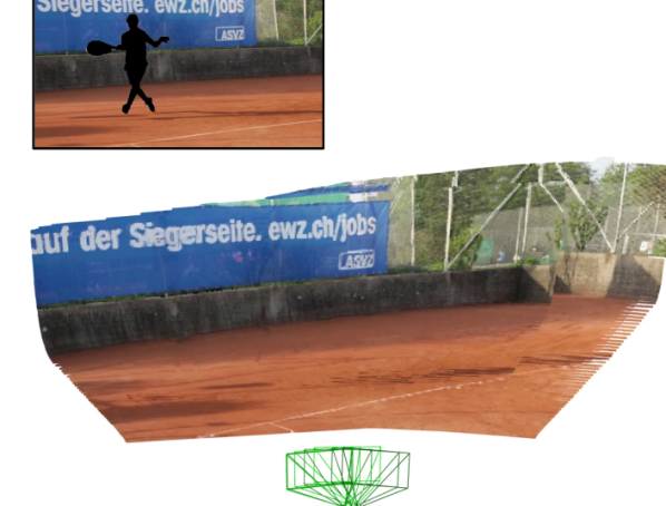
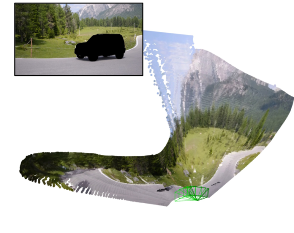
Pose and video depth
estimation

Rendering with
3D Gaussians [22]

Rendering with
Ours

Figure 2: 3D Gaussians [22] fails in weak-parallax videos. We show two casual videos in DAVIS [50] where the recent efficient 3D Gaussians produce floaters and noises in novel view due to insufficient parallax cues. We use the groundtruth masks to filter out the dynamic content and only reconstruct the static scenes.

We further develop a method and a set of loss functions to optimize our hybrid video representation from a monocular video. Since our hybrid representation can be rendered in real-time, our per-video optimization only takes 15 minutes on a single GPU. Our method achieves a rendering quality that is comparable to NeRF-based dynamic synthesis algorithms [14, 31, 38, 32] quantitatively and qualitatively, but is over 100x faster for training and rendering.

In summary, our contributions include:

• a hybrid explicit non-neural representation that can model both static and dynamic video content, support view-dependent effects and complex surface geometries, and enable real-time rendering;

• a per-video optimization algorithm together with a set of carefully designed loss functions to estimate the above hybrid video representation from a monocular video;

• extensive evaluations on the NVIDIA [78] and DAVIS datasets [50] show that our method can generate novel views with comparable quality to state-of-the-art NeRF-based view synthesis methods while being 100× faster for both training and rendering.

2 Related Work

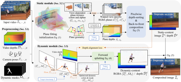
Figure 3: Method overview. We first preprocess an input monocular video to obtain obtain the video depth and pose as well as the dynamic masks (Sec. 3.1). The input video is then decomposed into static and dynamic content. We initialize a soup of oriented planes by fitting them to the static scene. These planes are augmented to capture view-dependent effects and non-planar complex surfaces. These planes are back-warped to the target view and composited from far to near to generate the target static view (Sec. 3.2). We estimate per-frame point clouds for dynamic content together with dynamic masks (Sec. 3.3). For temporal consistency, we use optical flows to blend the dynamic content from neighboring frames. The blended dynamic content is then warped to the target view. Finally, the target novel view is rendered by blending the static and dynamic novel content.

2.1 Dynamic-scene view synthesis

In contrast to static-scene novel view synthesis [17, 28, 58, 43, 44, 41, 33, 70, 64, 7, 42], novel view synthesis for dynamic scenes is particularly challenging due to the temporally varying contents that need to be handled. To make this problem more tractable, many existing methods [84, 63, 5, 4, 35, 52, 29, 2, 13, 9, 34, 40] reconstruct 4D scenes from multiple cameras capturing the dynamic scene simultaneously. However, such multi-view videos are not practical for casual applications, which instead only provide monocular videos. To tackle monocular videos, Yoon et al. [78] computes the video depth and performs depth-based 3D warping. However, the video depth may not be globally consistent, which results in view inconsistencies.

With the emergence of powerful neural rendering, a 4D scene can be implicitly represented in a neural network [76]. To model motion in neural representations,  [67, 14, 31, 47, 48, 61, 38] learn a canonical template with a deformation field to advect the casting rays. Some algorithms [14, 31, 38] utilize scene flow as a regularization for the 4D scene reconstruction which yield promising improvements. Instead of embedding a 4D scene within the network parameters, DynIBaR [32] aggregates the features from nearby views by a neural motion field to condition the neural rendering. Although existing neural rendering methods can achieve decent rendering quality, the computational costs and time for both per-scene training and rendering are high. Recently, MonoNeRF [66] and a concurrent work, FlowIBR [8], investigated priors in the form of pre-training on a large corpus of data to reduce the per-scene training time for neural rendering. While showing encouraging results, these approaches do not generalize well though and the time-consuming rendering is still present.

2.2 View synthesis with explicit representations

In contrast to implicitly encoding a scene in the network parameters, view synthesis algorithms with explicit 3D representations can often train and/or render faster.

Some methods exploit depth estimation to perform explicit 3D warping for novel view synthesis [46, 73, 78, 27, 10]. A feature-based point cloud is often used by neural rendering to enhance the synthesis quality [1, 73, 10, 56]. Instead of learning a feature space for point clouds, NPC [3] directly renders the RGB points with an MLP which yields a fast convergence and promising quality. Recent 3D/4D Gaussian approaches [22, 75] treat each 3D point as an anisotropic 3D Gaussian to learn and render high-quality novel views efficiently without neural rendering. Nevertheless, these methods heavily rely on accurate point locations for a global 3D point cloud. Therefore, they may require depth sensors [1] or SfM [57] as initialization [3, 22]. Based on an initial point cloud, subsequent approaches [22] leverage multi-view supervision to adaptively densify and prune the 3D points. However, these methods often fail in scenes with little parallax (Fig. 2).

Mesh is also a popular 3D representation [20]. However, it is difficult to estimate meshs from a casual video. One particular challenge is to directly optimize the positions of mesh vertices to integrate inconsistent depths from multiple views into a global mesh. Alternatively, [69, 71, 55, 77] first learn a neural SDF representation and then bake an explicit global mesh for static scenes. However, such a two-step method which involves optimizing for an MLP is slow.

Layered depth images (LDI) [58] are an efficient representation for novel view synthesis [59, 25, 30]. Multiplane image (MPI) approaches [83, 62, 68, 12, 74, 35, 49, 18], further extend the LDI representation and use a set of fronto-parallel RGBA planes to represent a static scene. These MPIs can often be generated using a feed-forward network and are thus fast to estimate. They can also be rendered efficiently by homography-based warping and alpha composition. However, fronto-parallel planes are restricted to forward-facing scenes and do not allow large viewpoint changes for novel view synthesis. To address this issue, [36, 80] construct a set of oriented feature planes to perform neural rendering for static-scene view synthesis. Yet again however, such feature planes require a time-consuming optimization. Our method, similarly inspired by [60], fits a soup of oriented planes to 3D scene surfaces. In contrast to feature planes, we adopt the non-neural RGBA representation in [83] for fast training and rendering.

   

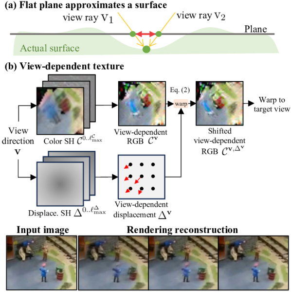
View-dep. appearance
View-dep. displacement

✗
✗

✓
✗

✓
✓

Figure 4: View-dependent texture. (a) Since a flat plane cannot sufficiently represent a non-flat surface, we augment it with both view-dependent appearance and displacement (b). Both of them are encoded by spherical harmonic coefficients, $\mathcal{C}^{0..{\ell_{\max}^{\mathcal{C}}}}$ and $\Delta^{0..{\ell_{\max}^{\Delta}}}$, respectively. Given a view direction $\mathbf{v}$, we first obtain the view-specific color $\mathcal{C}^{\mathbf{v}}$ and displacement $\Delta^{\mathbf{v}}$, then shift (backwarp) $\mathcal{C}^{\mathbf{v}}$ into the final view-specific $\mathcal{C}^{\mathbf{v},\Delta^{\mathbf{v}}}$ texture for planar homography warping to the target view. Note that the transparency map $\alpha$ is shifted jointly with $\mathcal{C}^{\mathbf{v}}$.

3 Method

As illustrated in Fig. 3, our method takes an $N$-frame RGB video, $\mathcal{I}_{1..N}$ as an input and renders a novel view $\tilde{\mathcal{I}}_{t}$ at the target view point $\tilde{T}$ and timestamp $t$. We first preprocess the input video to the obtain video depth maps $\mathcal{D}_{1..N}$, the camera trajectory $T_{1..N}$, and dynamic masks $\mathcal{M}_{1..N}$(Sec. 3.1). We then decompose the video into a global static representation (Sec. 3.2) and a per-frame dynamic representation (Sec. 3.3). Finally, we render the static and dynamic representations according to the target camera pose and composite them to generate the novel view $\tilde{\mathcal{I}}_{t}$.

We aim for a novel view synthesis approach that can train fast, support real-time rendering, and generate high-quality and temporally coherent novel views. As neural scene representations require more computation, we revisit explicit scene representations for a monocular video. First, we represent the dynamic content and the static background separately. We use a global background scene representation to enable temporally coherent view synthesis. To cope with dynamic content, we estimate a per-frame representation. While this is not ideal, minor inconsistencies within the dynamic content are not noticeable to viewers due to the motion-masking effect of human perception. Second, we use a soup of plane representation, inspired by Piecewise Planar Stereo [60], to represent the background and further extend it to support both view-dependent effects and non-planar scene surfaces. Third, we represent dynamic content using per-frame point clouds. As detailed later in this section, we provide a method that can efficiently estimate such a hybrid video representation to support real-time rendering of novel views with comparable quality of state-of-the-art methods that need 100× of our training time.

3.1 Preprocessing

Similar to existing methods [14, 31, 32], our method obtains an initial 3D reconstruction from an input video $\mathcal{I}_{1..N}$ using off-the-shelf video depth and pose estimation methods. Specifically, we use a re-implementation of RCVD [26] in VideoDoodles [79] to acquire video depth $\mathcal{D}_{1..N}$ and camera poses $T_{1..N}$. To obtain initial masks for dynamic regions, we first estimate likely-dynamic regions through semantic segmentation [19] and then acquire binarymotion masks by thresholding the error between optical flows [65] and rigid flows computed from depth maps and pose estimates. We then aggregate these masks to obtain the desired dynamic masks $\mathcal{M}_{1..N}$ before using Segment-Anything [24] to refine the object boundaries.

3.2 Extended Soup of Planes for Static Content

We fit a soup of oriented planes to the point cloud constructed using the pre-computed depth maps and camera poses in Sec. 3.1. To represent scene surfaces, each plane has the same texture resolution, which contains an appearance map and a density map. We further augment the planes with spherical harmonics and displacement fields to model view-dependent effects and non-planar surfaces.

Plane initialization. Given a number $N_{p}$ of finite planes $P_{1..N_{p}}$, we first fit them to the 3D static scene point cloud by minimizing the objective:

$$\small\Sigma_{i=1}^{N_{p}}d(P_{i},\mathbf{X}_{i,j})+\lambda_{norm}\langle\mathbf{n}_{P_{i}},\mathbf{n}_{\mathbf{X}_{i,j}}\rangle+\lambda_{area}w_{i}h_{i},$$ (1)

where each 3D point $\mathbf{X}_{j}$ is assigned to the nearest plane $P_{i}$ with finite size $(w_{i},h_{i})$ in every optimizing iteration. The point-to-plane distance is calculated by $d(P,\mathbf{X})=\sqrt{\max(|x^{P}|-\frac{w}{2},0)^{2}+\max(|y^{P}|-\frac{h}{2},0)^{2}+|z^{P}|^{2}},$ where $[x^{P},y^{P},z^{P}]^{\intercal}$ is the 3D point $\mathbf{X}$ w.r.t. the plane basis coordinate system with the plane center as the origin. We also measure the orientation difference between the point normal vector $\mathbf{n}_{\mathbf{X}_{i,j}}$ and the corresponding plane normal $\mathbf{n}_{P_{i}}$. The last term encourages each plane to have a compact size to avoid redundant overlapping planes. $\lambda_{norm}$, and $\lambda_{area}$ are hyper-parameters to re-weight each term.

View-dependent plane textures. A 2D plane texture stores $S\times S$ appearance $\mathcal{C}_{i}$ and transparency maps $\alpha_{i}$ of the corresponding 3D plane $P_{i}$. We utilize spherical harmonic (SH) coefficients for appearance maps to facilitate view dependency [53, 74, 22]. The view-specific color is obtained by $\mathcal{C}^{\mathbf{v}}=\sum_{\ell=0}^{\ell^{\mathcal{C}}_{\max}}\mathcal{C}^{\ell}H^{\ell}(\mathbf{v}),$ where $H^{\ell}$ are the SH basis functions. Moreover, a flat plane with a view-dependent appearance map may still be insufficient to represent a bumpy surface (Fig. 4a). The different viewing rays, $\mathbf{v}$, looking at the same 3D point may hit the plane in different locations, which can cause blurriness. To address this issue, we introduce a view-dependent displacement map $\Delta_{i}$ for each plane $P_{i}$, encoded by SH coefficients. As shown in Fig. 4b, given a ray $\mathbf{v}$, we obtain the view-specific displacement, $\Delta^{\mathbf{v}}=\sum_{\ell=0}^{\ell^{\Delta}_{\max}}\Delta^{\ell}H^{\ell}(\mathbf{v})$, to shift the color $\mathcal{C}^{\mathbf{v}}$ into $\mathcal{C}^{\mathbf{v},\Delta^{\mathbf{v}}}$:

$$\mathcal{C}^{\mathbf{v},\Delta^{\mathbf{v}}}(u,v)=\mathcal{C}^{\mathbf{v}}(u+\Delta^{\mathbf{v}}_{u},v+\Delta^{\mathbf{v}}_{v}),$$ (2)

where $(u,v)$ denotes the pixel on a plane that ray $\mathbf{v}$ hits. We also apply the displacement to the transparency map $\alpha$ along with color $\mathcal{C}^{\mathbf{v}}$, allowing a plane to better approximate the complex non-planar surface geometry.

Differentiable rendering. We first obtain the view-specific RGB $\mathcal{C}^{\mathbf{v},\Delta^{\mathbf{v}}}_{i}$ and transparency maps $\alpha^{\Delta^{\mathbf{v}}}_{i}$ from the texture of each plane $P_{i}$. We then backward warp them to the target view $\tilde{T}$ as $(\tilde{\mathcal{C}}^{\mathbf{v},\Delta^{\mathbf{v}}}_{i},\tilde{\alpha}^{\Delta^{\mathbf{v}}}_{i})$ using planar homography and composite them from back to front [83]. Unlike fronto-parallel MPIs that have a set of planes with fixed depth order [83], we need to perform pixel-wise depth sorting to the unordered and oriented 3D planes before compositing into the static-content image $\tilde{\mathcal{I}}^{s}$:

$$\tilde{\mathcal{I}}^{s}=\sum^{N_{p}}_{j=1}\left(\tilde{\mathcal{C}}^{\mathbf{v},\Delta^{\mathbf{v}}}_{j}\tilde{\alpha}^{\Delta^{\mathbf{v}}}_{j}\prod^{N_{p}}_{k=j+1}(1-\tilde{\alpha}^{\Delta^{\mathbf{v}}}_{k})\right).$$ (3)

Similarly, the static depth $\tilde{\mathcal{D}}^{s}$ can be obtained by replacing color $\tilde{\mathcal{C}}^{\mathbf{v},\Delta^{\mathbf{v}}}_{j}$ with plane depth $\tilde{d}_{j}$ in the above equation.

3.3 Consistent Dynamic Content Synthesis

Using oriented planes to represent near and complex dynamic objects is challenging. Therefore, we resort to simple but effective per-frame point clouds to represent them. At each timestamp $t$, we extract the dynamic appearance $\mathcal{I}^{d}_{t}$ and soft dynamic masks $\mathcal{M}^{*}_{t}$ from input frame $\mathcal{I}_{t}$ (Sec. 3.4). Then, they are warped to compute the dynamic color $\tilde{\mathcal{I}}^{d}_{t}$ and mask $\tilde{\mathcal{M}}_{t}$ at the target view $(\tilde{T},t)$ using forward splatting:

$$\tilde{\mathbf{x}}_{t}=\tilde{K}\tilde{T}T_{t}^{-1}\mathcal{D}_{t}K_{\tilde{t}}^{-1}\mathbf{x}_{t},$$ (4)

where $\mathbf{x}_{t}$ and $\tilde{\mathbf{x}}_{t}$ are pixel coordinates in the source $\mathcal{I}^{d}_{t}$ and target image $\tilde{\mathcal{I}}_{t}$, respectively. $K$ are the camera intrinsics. We adopt differentiable and depth-ordered softmax-splatting [45] to warp $(\mathcal{I}^{d}_{t},M^{*}_{t})$ to $(\tilde{\mathcal{I}}^{d}_{t},\tilde{M}_{t})$ as well as the dynamic depth $\tilde{D}^{d}_{t}$ w.r.t. view $\tilde{T}$. The final image $\tilde{\mathcal{I}}_{t}$ at $(\tilde{T},t)$ is blended by the static and dynamic content $(\tilde{\mathcal{I}}^{s},\tilde{\mathcal{I}}^{d}_{t})$:

$$\tilde{\mathcal{I}}_{t}=(1-\tilde{\mathcal{M}}^{\prime}_{t})\tilde{\mathcal{I}}^{s}+\tilde{\mathcal{M}}^{\prime}_{t}\tilde{\mathcal{I}}^{d}_{t},$$ (5)

where the soft mask $\tilde{\mathcal{M}}^{\prime}_{t}$ is based on the warped mask $\tilde{\mathcal{M}}_{t}$ and further considers the depth order between $\tilde{\mathcal{D}}^{s}_{t}$ and $\tilde{\mathcal{D}}^{d}_{t}$ to handle occlusions between them. Similarly, the final depth $\tilde{\mathcal{D}}_{t}$ can be computed from $\tilde{\mathcal{D}}^{s}_{t}$ and $\tilde{\mathcal{D}}^{d}_{t}$.

Temporal neighbor blending. Ideally, the dynamic appearance $\mathcal{I}^{d}_{t}$ and learned mask $\mathcal{M}^{*}_{t}$ can be optimized from the precomputed mask $\mathcal{M}_{t}$. But the precomputed mask $\mathcal{M}_{t}$ may be noisy and its boundary may be temporally inconsistent. As a result, extracting masks $\mathcal{M}^{*}_{1..N}$ independently from the noisy $\mathcal{M}_{1..N}$ can result in temporal inconsistencies. Therefore, we sample and blend the dynamic colors and masks from neighboring views $\mathcal{I}^{d}_{t\pm j}$ with $\mathcal{I}^{d}_{t}$ via the optical flow $\mathcal{F}_{t\to t\pm j}$ [65]. The blended dynamic color $\overline{\mathcal{I}}^{d}_{t}$ and mask $\overline{\mathcal{M}}_{t}$ are then warped to composite with static content.

Groundtruth

Ours

NSFF [31]

DynNeRF [14]

RoDynRF [38]

MonoNeRF$\dagger$ [66]

Figure 5: Visual comparison on the NVIDIA dataset. Our method can achieve comparable rendering quality for both static and dynamic content. Although our synthesized dynamic content may slightly misalign with the ground truth, resulting in lower PSNR, due to the ill-posed dynamic depth estimation problem, our results are sharp and perceptually similar to the ground truth. $\dagger$We reproduced MonoNeRF [66]’s per-scene optimization results by their official codes with the default configuration.

3.4 Optimization

Variables. We jointly optimize our hybrid static and dynamic video representation. For static content, in addition to the plane textures $(\mathcal{C}_{1..N_{p}},\alpha_{1..N_{p}},\Delta_{1..N_{p}})$, the precomputed camera poses $T_{1..N}$ and plane geometry (i.e., plane basis, center, width, and height) can also be optimized. For dynamic content, we first initialize the RGB and masks $(\mathcal{I}^{d}_{1..N},\mathcal{M}^{*}_{1..N})$ from the input frames $\mathcal{I}_{1..N}$ and precomputed masks $\mathcal{M}_{1..N}$ and then optimize them. Besides, we also refine flow $\mathcal{F}$ by fine-tuning flow model [65] for neighbor blending during the optimization. We also optimize the depth $\mathcal{D}^{d}_{1..N_{p}}$ for dynamic content when scene flow regularization is adopted. Then, we employ a recipe of reconstruction objectives and regularizations to assist optimization.

Photometric loss. The main supervision signal is the photometric difference between the rendered view $\tilde{\mathcal{I}}_{t}$ and the input frame $\mathcal{I}_{t}$ at view $T_{t}$. We omit time $t$ in this section for simplicity. The photometric loss $\mathcal{L}_{pho}$ is calculated as:

$$\mathcal{L}_{pho}(\tilde{\mathcal{I}},\mathcal{I})=(1-\gamma)\|\tilde{\mathcal{I}}-\mathcal{I}\|_{2}^{2}+\gamma\text{DSSIM}(\tilde{\mathcal{I}},\mathcal{I}),$$ (6)

where DSSIM is the structural dissimilarity loss based on the SSIM metric [72] with $\gamma=0.2$. Besides, the perceptual difference $\mathcal{L}_{pho}^{percep}$ [21] is also measured by a pretrained VGG16 encoder. Furthermore, to ensure the static plane textures represent static contents without dynamics picking any static content, we directly compute the masked static-content photometric loss between $\tilde{\mathcal{I}}^{s}$ and $\mathcal{I}$ by:

$$\mathcal{L}_{pho}^{s}=\min\left(\mathcal{L}_{pho}^{\mathcal{M}}(\tilde{\mathcal{I}}^{s},\mathcal{I}),\mathcal{L}_{pho}^{\mathcal{M}^{*}}(\tilde{\mathcal{I}}^{s},\mathcal{I})\right).$$ (7)

Dynamic mask. The soft dynamic mask $\mathcal{M}^{*}$ aims to blend the dynamic content $\mathcal{I}^{d}$ with the static content. We compute a cross entropy loss $\mathcal{L}_{mask}^{bce}$ between $\mathcal{M}^{*}$ and the precomputed mask $\mathcal{M}$ with a decreasing weight since $\mathcal{M}$ may be noisy. We also encourage the smoothness of $\mathcal{M}^{*}$ by an edge-aware smoothness loss $\mathcal{L}_{mask}^{smooth}$ [16]. To prevent the mask from picking static content, we apply a sparsity loss with both $L_{0}$- and $L_{1}$-regularizations [39] to restrict non-zero areas:

$$\small\mathcal{L}_{mask}^{reg}(\mathcal{M}^{*})=\mu_{0}\Phi_{0}(\mathcal{M}^{*})+\mu_{1}\|\mathcal{M}^{*}\|_{1}+\mu_{bce}L_{bce}(\mathcal{M}^{*},\mathbf{1}),$$ (8)

where $\Phi_{0}(\cdot)$ is an approximate $L_{0}$ [39]. For non-zero areas, we encourage them to be close to 1 via the binary cross entropy $L_{bce}(\cdot)$ with a small weight.

PSNR ↑/ LPIPS ↓	Jumping	Skating	Truck	Umbrella	Balloon1	Balloon2	Playground	Average
Yoon et al. [78]	20.15 / 0.148	21.75 / 0.135	21.53 / 0.099	20.35 / 0.179	18.74 / 0.179	19.88 / 0.139	15.08 / 0.184	19.64 / 0.152
Ours (10 frames)	22.60 / 0.107	29.23 / 0.049	22.68 / 0.079	22.58 / 0.109	22.98 / 0.088	23.56 / 0.087	21.39 / 0.083	23.57 / 0.086
D-NeRF* [52]	22.36 / 0.193	22.48 / 0.323	24.10 / 0.145	21.47 / 0.264	19.06 / 0.259	20.76 / 0.277	20.18 / 0.164	21.48 / 0.232
NR-NeRF* [67]	20.09 / 0.287	23.95 / 0.227	19.33 / 0.446	19.63 / 0.421	17.39 / 0.348	22.41 / 0.213	15.06 / 0.317	19.69 / 0.323
TiNeuVox* [11]	20.81 / 0.247	23.32 / 0.152	23.86 / 0.173	20.00 / 0.355	17.30 / 0.353	19.06 / 0.279	13.84 / 0.437	19.74 / 0.285
HyperNeRF* [48]	18.34 / 0.302	21.97 / 0.183	20.61 / 0.205	18.59 / 0.443	13.96 / 0.530	16.57 / 0.411	13.17 / 0.495	17.60 / 0.367
NSFF* [31]	24.65 / 0.151	29.29 / 0.129	25.96 / 0.167	22.97 / 0.295	21.96 / 0.215	24.27 / 0.222	21.22 / 0.212	24.33 / 0.199
DynNeRF* [14]	24.68 / 0.090	32.66 / 0.035	28.56 / 0.082	23.26 / 0.137	22.36 / 0.104	27.06 / 0.049	24.15 / 0.080	26.10 / 0.082
RoDynRF* [38]	25.66 / 0.071	28.68 / 0.040	29.13 / 0.063	24.26 / 0.089	22.37 / 0.103	26.19 / 0.054	24.96 / 0.048	25.89 / 0.065
MonoNeRF [66]	24.26 / 0.091	32.06 / 0.044	27.56 / 0.115	23.62 / 0.180	21.89 / 0.129	27.36 / 0.052	22.61 / 0.130	25.62 / 0.106
4D-GS [75]	21.93 / 0.269	24.84 / 0.174	23.02 / 0.175	21.83 / 0.213	21.32 / 0.185	18.81 / 0.178	18.40 / 0.196	21.45 / 0.199
Ours	23.45 / 0.100	29.98 / 0.045	25.22 / 0.090	23.24 / 0.096	23.75 / 0.079	24.15 / 0.081	22.19 / 0.074	24.57 / 0.081

Table 1: Quantitative comparison on the NVIDIA dataset [78]. We highlight the best and second best for each column. Yoon et al. [78]’s results only contain the middle 10 frames provided by RoDynRF [38]. * denotes the numbers reported by RoDynRF [38]. The per-scene optimization results of MonoNeRF [66] are adopted from their paper. The results of 4D-GS [75] are produced by their official codes. Our method achieves the second-best in the LPIPS metric.

Depth alignment. We use a depth loss to maintain the geometry prior in the precomputed $\mathcal{D}$ for the rendered depth $\tilde{\mathcal{D}}$ by $\mathcal{L}_{depth}=\|\tilde{\mathcal{D}}-\mathcal{D}\|_{1}/|\tilde{\mathcal{D}}+\mathcal{D}|$. Since the static depth $\tilde{\mathcal{D}}^{s}$ should align with the depth used for warping dynamic content for consistent static-and-dynamic view synthesis, we measure the error between static depth $\tilde{\mathcal{D}}^{s}$ and $\mathcal{D}$ similarly to the masked photometric loss in Eq. 7:

$$\mathcal{L}_{depth}^{s}=\min\left(\mathcal{L}_{depth}^{\mathcal{M}}(\tilde{\mathcal{D}}^{s},\mathcal{D}),\mathcal{L}_{depth}^{\mathcal{M}^{*}}(\tilde{\mathcal{D}}^{s},\mathcal{D})\right),$$ (9)

We also use the multi-scale depth smoothness regularization [16] for both full-rendered $\tilde{\mathcal{D}}$ and static depth $\tilde{\mathcal{D}}^{s}$.

Plane transparency smoothness. Relying solely on smoothing composited depths is insufficient to smooth the geometry in 3D space. Therefore, we further apply a total variation loss $L_{\alpha}^{tv}$ to each warped plane transparency $\tilde{\alpha}^{\Delta^{\mathbf{v}}}_{i}$.

Scene flow regularization. Depth estimation for dynamic content in a monocular video is an ill-posed problem. Many existing methods first estimate depth maps for individual frames with a single-image depth estimation method. They then assume that the motion is slow and accordingly use scene flows as regularization to smooth the individually estimated depth maps to improve the temporal consistency. However, it still highly depends on the initial single depth estimates. We observe that the assumption may not always hold true and may compromise the scene reconstruction and novel view synthesis quality. In addition, scene flow regularization slows our training process significantly. Hence, we disable scene flow regularization by default. We will discuss the effect of the scene flow regularization in the supplemental material. Another promising solution is to preprocess depth maps in true scale [6] to provide reliable dynamic-object depth, which we will explore in the future.

Implementation details. Our implementation is based on PyTorch with Adam [23] and VectorAdam [37] optimizers along with a gradient scaler [51] to prevent floaters. We follow 3D Gaussians [22] to gradually increase the number of bands in SH coefficients during optimization. The optimization only takes 15 minutes on a single A100 GPU with 2000 iterations. We describe our detailed hyper-parameter settings in the supplemental material.

4 Experimental Results

We experiment with our methods and compare to SOTA on NVIDIA Dynamic Scene [78] and DAVIS [50] datasets.

4.1 Comparisons on the NVIDIA Dataset

NVIDIA’s Dynamic Scene Dataset [78] contains 9 scenes simultaneously captured by 12 cameras on a static camera rig. To simulate a monocular input video with a moving camera, we follow the protocol in DynNeRF [14] to pick a non-repeating camera view for each timestamp to form a 12-frame video. We measure the PSNR and LPIPS [81] scores on the novel views from the viewpoint of the first camera but at varying timestamps. We show the visual comparisons in Fig. 5 and report quantitative results in Table 1. Although our PSNR scores are slightly worse than NSFF [31] in some sequences, our LPIPS scores are consistently better. This is because depth estimation for dynamic content is ill-posed. A slightly inaccurate dynamic depth can cause a slight misalignment between the ground truth and the rendered image. The pixel-wise PSNR metric is sensitive to such subtle misalignments while we argue that LPIPS is a fairer metric for monocular dynamic view synthesis since it measures the perceptual difference rather than pixel-wise errors. Besides, even though MonoNeRF [66] has shown generalization potential by pre-training on one scene and fine-tuning on a target scene, our approach still performs better than its per-scene optimization setting. Overall, our method achieves the second-best LPIPS and comparable PSNR scores but with over 100× faster training and rendering speeds than [38, 14, 31].

Groundtruth

Ours

NSFF [31]

DynNeRF [14]

DynIBaR [32]

Figure 6: Visual comparison on NVIDIA-long protocol [32]. While the dynamic content in our results slightly misaligns with the ground truth due to the ill-posed dynamic depth estimation problem, our results are sharp with richer details than [31, 14].

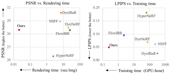
Figure 7: Quantitative and speed comparison using the NVIDIA-long protocol [32]. Although DynIBaR [32] gets the best quality overall, it is time-consuming for training and rendering. In contrast, with the fastest training and rendering speed, the rendering quality of our method is the second-best in the LPIPS metric, and comparable with DynNeRF [14] and NSFF [31] and better than FlowIBR [8] in the PSNR metric.

Method	Training	Rendering (sec/img)		NVIDIA LPIPS↓
	GPU hour	480×270	860×480
Yoon et al. $\dagger$ [78]	>2	-	>1	0.152
HyperNeRF* [48]	64	2.5	-	0.367
DynNeRF* [14]	74	20.4	-	0.082
NSFF* [31]	223	6.2	-	0.199
RoDynRF [38]	28	2.4	7.6	0.065
DynIBaR [32]	320	7.2	22.2	-
FlowIBR* [8]	2.3	25.1	-	-
MonoNeRF [66]	22	22.9	76.9	0.106
4D Gaussians [75]	1.2	0.023	0.035	0.199
Ours	0.25	0.021	0.038	0.081

Table 2: Speed comparison. Our method achieves real-time rendering and the second-best LPIPS score on the NVIDIA Dataset [78]. $\dagger$We corresponded with the authors of [78] to acquire the runtime performance. * denotes the speeds reported by [8].

To compare with DynIBaR, we followed their protocol to form longer input videos with 96-204 frames by repeatedly sampling from the 12 cameras [32]. The overall quantitative scores and time comparisons are presented in Fig. 7. Again, due to the ill-posed dynamic depth and only relying on video depth without scene flow regularization, our method produces slight misalignments with respect to the ground truth in dynamic areas and thus yields slightly worse PSNR scores. Nevertheless, as shown in Fig. 6, our approach provides sharper and richer details in dynamic content than NSFF [31] and DynNeRF [14] and accordingly, our method achieves the second-best LPIPS score.

4.2 Visual Comparisons on the DAVIS Datatset

The videos generated from the NVIDIA dataset [14] is different from an in-the-wild video. Therefore, we select several videos from the DAVIS Dataset [50] to validate our algorithm in real-world scenarios. For a fair comparison, we use the same video depth and pose estimation from our preprocessing step for DynIBaR and then run DynIBaR with their officially released code [32]. We show the results in Fig. 8. Although DynIBaR can synthesize better details with neural rendering in the first example, it introduces blurriness by aggregating information from local frames and yields noticeable artifacts in other three examples. In contrast, our method maintains a static scene representation and obtains comparable quality to DynIBaR in the first example while being significantly faster to train and render.

4.3 Speed Comparisons

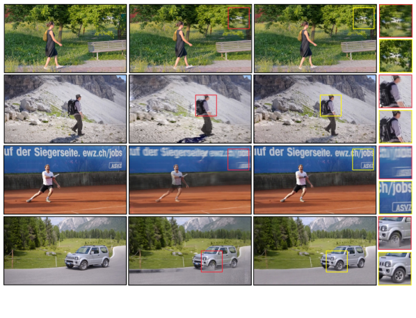
Input

DynIBaR [32]

Ours

Figure 8: Visual comparison on DAVIS [50]. We showcase the novel view synthesis results and the corresponding input frame at the same time. DynIBaR [32] may fail to handle some casual videos with few parallax and introduce noticeable artifacts.

We compare both per-scene training and rendering speed in Table 2 along with the overall LPIPS scores in Table 1. NeRF-based methods [31, 14, 38] usually require multiple GPUs and/or over one day for the per-video optimization. While some recent studies [8, 66] attempt to develop a generalized NeRF-based approach, there is still a quality gap to the per-video optimization methods, and their rendering speed is still slow. In contrast, explicit representations, such as our method and 4D-GS [75], can train and render fast. Our method has a similar rendering speed but is faster to optimize than 4D-GS. In summary, our method can generate novel views with comparable quality to NeRF-based methods while being much faster to train and render (both >100× faster than [38, 32]).

4.4 Ablation Study

To thoroughly examine our method, we conduct ablation studies on the NVIDIA Dataset in Table 3. In our static module, the view dependency of plane textures plays a key role in rendering quality. The individual view-dependent appearance and displacement can each enhance the LPIPS scores by 19% (0.104→0.084) and 16% (0.104→0.087), respectively. Jointly, they can improve the baseline further, 22% in LPIPS and 1.4dB in PSNR. For the dynamic module, the improvement by adding neighboring blending is not significant since the preprocessed masks are already good as provided by DynNeRF’s protocol [14]. We encourage the readers to view our supplementary videos to observe the improved temporal consistency on casual videos.

Ablation setting		PSNR↑	LPIPS↓
Static	w/o view-dep. appear. and displace.	23.14	0.104
	w/o view-dep. appear.	24.05	0.087
	w/o view-dep. displace.	24.34	0.084
Dynamic	w/o temporal neighbor blending	24.48	0.081
Ours (full)		24.57	0.081

Table 3: Ablation study. For static content, both view-dependent appearance $\mathcal{C}$ and displacement maps $\Delta$ improve the synthesis quality. For dynamic content, the improvement is not significant due to the already good preprocessed masks provided by DynNeRF’s protocol [14]. We encourage readers to view our supplementary videos to see the improved temporal consistency.

Figure 9: Limitations. Our view synthesis quality may degrade when the preprocessed video depth (b) is inaccurate. The subtle motion of dynamic content makes motion segmentation difficult, leaking dynamic content into the static representations (c). Similar to DynIBaR [32], our method may produce incomplete dynamic content (e) due to the per-frame representation for dynamics.

 

4.5 Limitations

Our approach may fail when the preprocessed video depth and pose are inaccurate. As shown in Fig. 9c, the static scene reconstruction is blurry because the inaccurate depth estimation leads to a poor initialization of the oriented planes. In addition, our method cannot separate objects with subtle motion from a static background, such as videos in DyCheck [15], which is a challenging dataset for most of the state-of-the-art methods. Besides, similar to DynIBaR [32], our method may produce an incomplete foreground (Fig. 9e) by forward splatting from the local source frame without a canonical dynamic template.

5 Conclusions

This paper presented an efficient view synthesis method for casual videos. Similar to state-of-the-art methods, we adopted a per-video optimization strategy to achieve high-quality novel view synthesis. To speed up our training / optimization process, instead of using a NeRF-based representation, we revisit explicit representations and used a hybrid static-dynamic video representation. We employed a soup of planes as a global static background representation. We further augmented it using spherical harmonics and displacements to enable view-dependent effects and model complex non-planar surface geometry. We use per-frame point clouds to represent dynamic content for efficiency. We further developed an effective optimization method together with a set of carefully designed loss functions to optimize for such a hybrid video representation from an in-the-wild video. Our experiments showed that our method can generate high-quality novel views with comparable quality to state-of-the-art NeRF-based approaches while being (>100×) for both training and testing.

Appendix

We present further details of our method implementation (Sec. A), runtime analysis of our method (Sec. B), additional visual comparisons on the NVIDIA dataset [78] (Sec. C), and the discussion of scene flow regularization (Sec. D)

Appendix A Implementation details

A.1 Initialization.

Plane geometry. As described in the Sec. 3.2 of the main paper, we fit a soup of oriented 3D planes to the scene surfaces by a simple optimization with the objective Eq. (1) in the main paper. We first obtain the static scene point cloud by unprojecting the depth estimation from a set of keyframes, which are selected by a fixed stride (e.g., 4). Subsequently, to initialize the planes’ positions before the fitting optimization, we randomly sample $N_{p}$ points from the point cloud as plane centers, where the randomness is weighted by the inverse of points’ depths (i.e., disparities). The intuition is that the nearer scenes may need more planes to represent more details with complex depths. Similarly, the nearer planes are initialized with smaller sizes to maintain fidelity since all planes have the same texture resolution. The fitting process is effective at distributing the $N_{p}$ planes to fit the entire scene surface (as shown in Fig. 3 in the main paper). We set the number of planes $N_{p}=64$ by default and 5000 iterations for the fitting optimization. And the hyper-parameters $\lambda_{norm}$ and $\lambda_{area}$ in Eq. (1) in the main paper are set as $10^{6}$ and $10^{-4}$, respectively.

Plane texture. Once the plane fitting optimization is completed, we can initialize the base color $\mathcal{C}^{0}_{1..N_{p}}$ and transparency $\alpha_{1..N_{p}}$ for the view-dependent plane textures. With the per-frame RGB point cloud, we assign the pixel color and transparency as 1 at the intersection of the viewing ray and the plane that is nearest to the point. For casual videos, we set the width $S=256$ for each plane texture. The degree of spherical harmonics (SH) coefficients for view-dependent color $\ell^{\mathcal{C}}_{\max}$ is set to 3. For the view-dependent displacement maps $\Delta_{1..N_{p}}$, we initialize it with zeros (i.e., no displacement). The width of displacement maps is set to $32$ with SH degree $\ell^{\Delta}_{\max}$ = 2. We use a sigmoid as the activation function for the transparency maps $\alpha_{1..N_{p}}$ to limit the range to $[0,1]$.

Rendering step		Runtime (ms)
Static	Obtain view-dep. texture	1.99
	Plane warping	12.42
	Pixelwise depth sorting	0.12
	Plane composition	0.27
Dynamic	Neighboring blending	21.28
	Forward splatting	1.35
Static-dynamic composition		0.09
Total		37.52

Table 4: Rendering runtime breakdown. The experiment is conducted on a single A100 GPU with an 80-frame input video of 860×480 resolution. The proposed method achieves real-time rendering at 27 FPS.

Training step		Runtime (sec)
Initialization	Plane geometry fitting	22.2
	Plane texture	1.2
	Dynamic model	2.4
Synthesis Optimization		782.0
Total		807.8

Table 5: Training runtime breakdown. We run the experiment on a single A100 GPU with an 80-frame input video of 860x480 resolution. Our method is efficient to supervise and trains on casual videos within 15 minutes.

Dynamic module. The initial per-frame dynamic colors $I^{d}_{1..N}$ are extracted from the input frames $I_{1..N}$ using the preprocessed binary masks $\mathcal{M}_{1..N}$. Besides, the depth for dynamic-content splatting is initialized with the precomputed depth $\mathcal{D}_{1..N}$ and can be updated when the scene flow regularization is adopted.

A.2 Synthesis Optimization.

The synthesis optimization yields one image per iteration (i.e., batch size = 1). For casual videos of frames with a 860×480 resolution and $\sim$100 frames, we use 1000 iterations by default. For the NVIDIA dataset [78] with a resolution of 480×270, the number of iterations is set to 2000. Both training processes can be completed within 15 minutes. For the view-dependent plane textures in the static module, The active bands of the SH coefficients are increased every 50 iterations until reaching the maximum SH degrees [22].

In the dynamic module, we take the neighbors $\{t\pm 1,t\pm 2\}$ of the source view at the timestamp ${t}$ for temporal neighbor blending. We utilize the pretrained backbone of the MiDaS network [54] to learn the dynamic masks $\mathcal{M}^{*}_{1..N_{p}}$. The RAFT model [65] is jointly fine-tuned with a photometric loss $\mathcal{L}_{flow}^{pho}$ and a cycle consistency loss $\mathcal{L}_{flow}^{cycle}$ to obtain the refined optical flow $\mathcal{F}$ for the neighbor blending. We exploit a small MLP with positional encoding to output a grid of scales and shifts to adjust the dynamic depth $\mathcal{D}^{d}_{t}$ when the scene flow regularization is applied. Note that the rendering phase does not require any network pass since we can directly use the network outputs (i.e., masks $\mathcal{M}^{*}$, flows $\mathcal{F}$, dynamic depths $\mathcal{D}^{d}$) on the fly.

The total loss $\mathcal{L}$ is computed by:

$$\mathcal{L} =\mathcal{L}^{total}_{pho}+\mathcal{L}^{total}_{mask}+\mathcal{L}^{total}_{depth}$$ (10)

$$+\eta_{flow}\mathcal{L}^{total}_{flow}+\eta_{\alpha}\mathcal{L}_{\alpha}^{tv},$$

$$\mathcal{L}^{total}_{pho} =\rho_{full}\mathcal{L}_{pho}+\rho_{s}\mathcal{L}_{pho}+\rho^{percep}\mathcal{L}^{percep}_{pho},$$

$$\mathcal{L}^{total}_{mask} =\mu_{preproc}\mathcal{L}^{bce}_{mask}+\mathcal{L}^{reg}_{mask}+\mu_{smooth}\mathcal{L}^{smooth}_{mask},$$

$$\mathcal{L}^{total}_{depth} =\sigma_{full}\mathcal{L}_{depth}+\sigma_{s}\mathcal{L}^{s}_{depth}$$

$$+\sigma_{smooth}\mathcal{L}^{smooth}_{depth}+\sigma_{smooth,s}\mathcal{L}^{smooth,s}_{depth},$$

$$\mathcal{L}^{total}_{flow} =\mathcal{L}^{pho}_{flow}+\mathcal{L}^{cycle}_{flow}$$

where the hyper-parameters for the photometric loss $\rho_{full},\rho_{s},\rho_{percep}=10,10,1$, respectively. For the mask loss $\mathcal{L}_{mask}^{total}$, $\mu_{preproc}=0.05$, $\mu_{0}=1.5$, the hyper-parameters $\mu_{1}=0.0015$, and $\mu_{bce}=0.5$, corresponding to the Eq. (8) in the main paper. For the depth loss $\mathcal{L}_{depth}^{total}$, we compute the errors on the full-rendered depth $\tilde{\mathcal{D}}$ and $\tilde{\mathcal{D}}^{s}$. Similarly, the smoothness losses $\mathcal{L}^{smooth}_{depth}$ and $\mathcal{L}^{smooth,s}_{depth}$ are considered. The hyper-parameters are set as $\sigma_{full}=0.1$, $\sigma_{s}=0.1$, $\sigma_{smooth}=1$, $\sigma_{smooth,s}=0.1$. Lastly, the hyper-parameters for the flow loss $\mathcal{L}_{flow}^{total}$ and the smoothness loss of plane transparency $\mathcal{L}_{\alpha}^{tv}$ are $\eta_{flow}=10$ and $\eta_{\alpha}=10$, respectively.

A.3 Rendering.

To achieve fast view synthesis, we save all outputs of the trained networks after the synthesis optimization. Consequently, the rendering phase does not require any network pass and directly takes the saved outputs on the fly. The saved parameters take roughly 1.4GB for an 80-frame video. In addition, only the neighbors $\{t\pm 1\}$ of the source view at timestamp $t$ are used for temporal neighbor blending in order to speed up the rendering.

Appendix B Runtime analysis

We present the runtime breakdown of both the rendering and training processes in Table 4 and Table 5, respectively. The experiments are run on a single A100 GPU with an 80-frame input video of 860×480 resolution. Our proposed method performs efficient training on an input video within 15 minutes and real-time rendering at 27 FPS.

Appendix C Visual comparisons on the NVIDIA dataset

We present additional visual comparisons on the NVIDIA dataset [78] using DynNeRF [14]’s evaluation protocol. The results of HyperNeRF [48], NSFF [31], DynNeRF [14], and RoDynRF [38] are provided by RoDynRF [38]. For MonoNeRF [66], we re-produced the pre-scene optimization results by using the officially-released codes with the default configuration.

As shown in Fig. 10 and Fig. 11, HyperNeRF [48] and 4D-GS [75] fail to capture the motion with their deformation fields and yield severe distortions and artifacts. MonoNeRF [66] produces duplicated dynamic content in both examples of Fig. 11. Besides, in the second example of Fig. 10, DynNeRF [14] and MonoNeRF [66] introduce noise to the green pole on the left. Our proposed method can render high-quality results with the fastest training and rendering speeds.

Appendix D Scene flow regularization

Due to the ill-posed dynamic-depth estimation problem, the scene flow regularization is usually adopted [31, 14, 38, 32] to learn a smooth motion field from per-frame depths and optical flows. Subsequently, the rendering is performed by the learned motion field. Notably, unlike the neural-rendering approaches that aim to acquire smoothed neural motion fields, our explicit approach attempts to obtain the smoothed dynamic depths for rendering. Therefore, similar to Zhang et al. [82] used in the preprocessing of DynIBaR [32], scene flow regularization is also adopted in our preprocessing video depth and pose estimation. In addition, we further apply the scene flow to the optimization of our synthesis framework.

D.1 Method details of scene flow regularization

To smooth the motion in the sequential dynamic depth maps, the dynamic depth $\mathcal{D}^{d}_{1..N}$ is updated by scene flow regularization $\mathcal{L}_{sf}^{depth}$ through the optimization:

$$\mathcal{L}_{sf}^{depth}=\frac{\|\mathcal{D}_{t}^{d}-z_{t+j\to t}\|_{1}}{|\mathcal{D}_{t}^{d}+z_{t+j\to t}|},$$ (11)

where $z_{t+j\to t}$ denotes the z-component of the scene flow $\mathbf{X}_{t+j\to t}$ from timestamp $t+j$ to $t$, w.r.t. the view $t$. To estimate the scene flow, we follow [82] exploiting an MLP $\theta_{sf}$ to predict the forward and backward motions of an input 3D point $\mathbf{X}_{t}$ at time $t$:

$$(\mathbf{X}_{t\to t+1},\mathbf{X}_{t\to t-1})=\theta_{sf}(\mathbf{X}_{t},t).$$ (12)

We compute the cycle-consistency loss $\mathcal{L}_{sf}^{cycle}$ of the scene flow estimation as well as the error $\mathcal{L}_{sf}^{flow}$ between the precomputed optical flow [65] and the inferred flow of projecting $\mathbf{X}_{t\to t+1}$ to the 2D image plane. The scene flow is smoothed by:

$$\mathcal{L}_{sf}^{smooth}=\sum^{t+\omega-1}_{i=t-\omega+1}\|X_{i-1\to i}-X_{i\to i+1}\|_{2},$$ (13)

where $\omega$ is half of the window size of the scene flow track. We set $\omega=2$. Finally, the entire scene flow loss $\mathcal{L}_{sf}=\mathcal{L}_{sf}^{flow}+\beta_{depth}\mathcal{L}_{sf}^{depth}+\beta_{cycle}\mathcal{L}_{sf}^{cycle}+\beta_{smooth}\mathcal{L}_{sf}^{smooth}$ is then added the total loss $\mathcal{L}$, where we set $\beta_{depth}=10^{-3}$, $\beta_{cycle}=10^{-2}$, and $\beta_{smooth}=10^{-3}$.

D.2 Results with adding scene flow regularization

With the scene flow regularization $\mathcal{L}_{sf}$, we can observe the improvements on 3 sequences on the Nvidia dataset [78] in Table 6. Nevertheless, the synthesis quality degrades in the other 4 sequences due to some distortions in the over-smoothed dynamic depth $\mathcal{D}^{d}_{1..N}$. We found that the adjustment of dynamic depth maps is still highly affected by the initial depth estimates, and therefore it is not easy to obtain the ideal depth that aligns with the actual groundtruth in practice. Furthermore, the scene flow regularization slows the synthesis optimization process (15 → 33 minutes). As a result, we disable the scene flow regularization in our synthesis optimization by default. Despite some slight misalignments with the ground truth, our method can still yield visually plausible synthesis results. To solve the ill-posed dynamic depth problem, a promising future direction is to improve the accuracy of single-depth estimators in true scale [6].

Ground Truth

Ours

HyperNeRF [14]

NSFF [31]

DynNeRF [14]

RoDynRF [38]

MonoNeRF [66]

4D-GS [75]

Groundt Truth

Ours

HyperNeRF [14]

NSFF [31]

DynNeRF [14]

RoDynRF [38]

MonoNeRF [66]

4D-GS [75]

Ground Truth

Ours

HyperNeRF [14]

NSFF [31]

DynNeRF [14]

RoDynRF [38]

MonoNeRF [66]

4D-GS [75]

Figure 10: Visual comparison on the NVIDIA dataset.

Ground Truth

Ours

HyperNeRF [14]

NSFF [31]

DynNeRF [14]

RoDynRF [38]

MonoNeRF [66]

4D-GS [75]

Ground Truth

Ours

HyperNeRF [14]

NSFF [31]

DynNeRF [14]

RoDynRF [38]

MonoNeRF [66]

4D-GS [75]

Figure 11: Visual comparison on the NVIDIA dataset.

PSNR ↑/ LPIPS ↓	Train time	Jumping	Skating	Truck	Umbrella	Balloon1	Balloon2	Playground	Average
Ours w/ $\mathcal{L}_{sf}$	33 min	22.36 / 0.121	28.99 / 0.062	25.07 / 0.093	23.91 / 0.094	22.36 / 0.121	25.31 / 0.072	22.76 / 0.070	24.55 / 0.086
Ours w/o $\mathcal{L}_{sf}$	15 min	23.45 / 0.100	29.98 / 0.045	25.22 / 0.090	23.24 / 0.096	23.75 / 0.079	24.15 / 0.081	22.19 / 0.074	24.57 / 0.081

Table 6: Ablation on scene flow regularization. Although the scene flow regularization $\mathcal{L}_{sf}$ can improve the scores of three examples by better aligning with the ground-truths, the quality of the other four examples degrades due to the over-smoothed dynamic depths caused by the regularization. Additionally, the scene flow regularization doubles the training time. Hence, we disable the scene flow regularization by default. Without the regularization, our method can still render visually plausible dynamics in spite of some slight misalignments with the ground truth. We encourage our readers to view our demo webpage to see the video synthesis results of casual videos.

References

- Aliev et al. [2020] Kara-Ali Aliev, Artem Sevastopolsky, Maria Kolos, Dmitry Ulyanov, and Victor Lempitsky. Neural point-based graphics. In ECCV, 2020.
- Attal et al. [2023] Benjamin Attal, Jia-Bin Huang, Christian Richardt, Michael Zollhoefer, Johannes Kopf, Matthew O’Toole, and Changil Kim. HyperReel: High-fidelity 6-DoF video with ray-conditioned sampling. In CVPR, 2023.
- Bansal and Zollhoefer [2023] Aayush Bansal and Michael Zollhoefer. Neural pixel composition for 3d-4d view synthesis from multi-views. In CVPR, 2023.
- Bansal et al. [2020] Aayush Bansal, Minh Vo, Yaser Sheikh, Deva Ramanan, and Srinivasa Narasimhan. 4d visualization of dynamic events from unconstrained multi-view videos. In CVPR, 2020.
- Bemana et al. [2020] Mojtaba Bemana, Karol Myszkowski, Hans-Peter Seidel, and Tobias Ritschel. X-fields: Implicit neural view-, light- and time-image interpolation. SIGGRAPH Asia, 2020.
- Bhat et al. [2023] Shariq Farooq Bhat, Reiner Birkl, Diana Wofk, Peter Wonka, and Matthias Müller. Zoedepth: Zero-shot transfer by combining relative and metric depth. arXiv preprint arXiv:2302.12288, 2023.
- Bian et al. [2023] Wenjing Bian, Zirui Wang, Kejie Li, Jia-Wang Bian, and Victor Adrian Prisacariu. Nope-nerf: Optimising neural radiance field with no pose prior. In CVPR, 2023.
- Büsching et al. [2023] Marcel Büsching, Josef Bengtson, David Nilsson, and Mårten Björkman. Flowibr: Leveraging pre-training for efficient neural image-based rendering of dynamic scenes. arXiv preprint arXiv:2309.05418, 2023.
- Cao and Johnson [2023] Ang Cao and Justin Johnson. Hexplane: A fast representation for dynamic scenes. CVPR, 2023.
- Cao et al. [2022] Ang Cao, Chris Rockwell, and Justin Johnson. Fwd: Real-time novel view synthesis with forward warping and depth. CVPR, 2022.
- Fang et al. [2022] Jiemin Fang, Taoran Yi, Xinggang Wang, Lingxi Xie, Xiaopeng Zhang, Wenyu Liu, Matthias Nießner, and Qi Tian. Fast dynamic radiance fields with time-aware neural voxels. In SIGGRAPH Asia 2022 Conference Papers, 2022.
- Flynn et al. [2019] John Flynn, Michael Broxton, Paul Debevec, Matthew DuVall, Graham Fyffe, Ryan Overbeck, Noah Snavely, and Richard Tucker. Deepview: View synthesis with learned gradient descent. In CVPR, 2019.
- Fridovich-Keil et al. [2023] Sara Fridovich-Keil, Giacomo Meanti, Frederik Rahbæk Warburg, Benjamin Recht, and Angjoo Kanazawa. K-planes: Explicit radiance fields in space, time, and appearance. In CVPR, 2023.
- Gao et al. [2021] Chen Gao, Ayush Saraf, Johannes Kopf, and Jia-Bin Huang. Dynamic view synthesis from dynamic monocular video. In ICCV, 2021.
- Gao et al. [2022] Hang Gao, Ruilong Li, Shubham Tulsiani, Bryan Russell, and Angjoo Kanazawa. Monocular dynamic view synthesis: A reality check. In NeurIPS, 2022.
- Godard et al. [2017] Clément Godard, Oisin Mac Aodha, and Gabriel J Brostow. Unsupervised monocular depth estimation with left-right consistency. In CVPR, 2017.
- Gortler et al. [1996] Steven J. Gortler, Radek Grzeszczuk, Richard Szeliski, and Michael F. Cohen. The lumigraph. In SIGGRAPH, 1996.
- Han et al. [2022] Yuxuan Han, Ruicheng Wang, and Jiaolong Yang. Single-view view synthesis in the wild with learned adaptive multiplane images. In SIGGRAPH, 2022.
- He et al. [2017] Kaiming He, Georgia Gkioxari, Piotr Dollár, and Ross Girshick. Mask r-cnn. In ICCV, 2017.
- Hu et al. [2021] Ronghang Hu, Nikhila Ravi, Alexander C. Berg, and Deepak Pathak. Worldsheet: Wrapping the world in a 3d sheet for view synthesis from a single image. In ICCV, 2021.
- Johnson et al. [2016] Justin Johnson, Alexandre Alahi, and Li Fei-Fei. Perceptual losses for real-time style transfer and super-resolution. In ECCV, 2016.
- Kerbl et al. [2023] Bernhard Kerbl, Georgios Kopanas, Thomas Leimkühler, and George Drettakis. 3d gaussian splatting for real-time radiance field rendering. ACM TOG, 2023.
- Kingma and Ba [2015] Diederik P. Kingma and Jimmy Ba. Adam: A method for stochastic optimization. In ICLR, 2015.
- Kirillov et al. [2023] Alexander Kirillov, Eric Mintun, Nikhila Ravi, Hanzi Mao, Chloe Rolland, Laura Gustafson, Tete Xiao, Spencer Whitehead, Alexander C. Berg, Wan-Yen Lo, Piotr Dollár, and Ross Girshick. Segment anything. arXiv:2304.02643, 2023.
- Kopf et al. [2020] Johannes Kopf, Kevin Matzen, Suhib Alsisan, Ocean Quigley, Francis Ge, Yangming Chong, Josh Patterson, Jan-Michael Frahm, Shu Wu, Matthew Yu, Peizhao Zhang, Zijian He, Peter Vajda, Ayush Saraf, and Michael Cohen. One shot 3d photography. In SIGGRAPH, 2020.
- Kopf et al. [2021] Johannes Kopf, Xuejian Rong, and Jia-Bin Huang. Robust consistent video depth estimation. In CVPR, 2021.
- Lee et al. [2021] Yao-Chih Lee, Kuan-Wei Tseng, Yu-Ta Chen, Chien-Cheng Chen, Chu-Song Chen, and Yi-Ping Hung. 3d video stabilization with depth estimation by cnn-based optimization. In CVPR, 2021.
- Levoy and Hanrahan [1996] Marc Levoy and Pat Hanrahan. Light field rendering. In SIGGRAPH, 1996.
- Li et al. [2022] Tianye Li, Mira Slavcheva, Michael Zollhoefer, Simon Green, Christoph Lassner, Changil Kim, Tanner Schmidt, Steven Lovegrove, Michael Goesele, Richard Newcombe, et al. Neural 3d video synthesis from multi-view video. In CVPR, 2022.
- Li et al. [2023a] Xingyi Li, Zhiguo Cao, Huiqiang Sun, Jianming Zhang, Ke Xian, and Guosheng Lin. 3d cinemagraphy from a single image. In CVPR, 2023a.
- Li et al. [2021] Zhengqi Li, Simon Niklaus, Noah Snavely, and Oliver Wang. Neural scene flow fields for space-time view synthesis of dynamic scenes. In CVPR, 2021.
- Li et al. [2023b] Zhengqi Li, Qianqian Wang, Forrester Cole, Richard Tucker, and Noah Snavely. Dynibar: Neural dynamic image-based rendering. In CVPR, 2023b.
- Lin et al. [2021a] Chen-Hsuan Lin, Wei-Chiu Ma, Antonio Torralba, and Simon Lucey. Barf: Bundle-adjusting neural radiance fields. In ICCV, 2021a.
- Lin et al. [2023] Haotong Lin, Sida Peng, Zhen Xu, Tao Xie, Xingyi He, Hujun Bao, and Xiaowei Zhou. High-fidelity and real-time novel view synthesis for dynamic scenes. In SIGGRAPH Asia Conference Proceedings, 2023.
- Lin et al. [2021b] Kai-En Lin, Lei Xiao, Feng Liu, Guowei Yang, and Ravi Ramamoorthi. Deep 3d mask volume for view synthesis of dynamic scenes. In ICCV, 2021b.
- Lin et al. [2022] Zhi-Hao Lin, Wei-Chiu Ma, Hao-Yu Hsu, Yu-Chiang Frank Wang, and Shenlong Wang. Neurmips: Neural mixture of planar experts for view synthesis. In CVPR, 2022.
- Ling et al. [2022] Selena Zihan Ling, Nicholas Sharp, and Alec Jacobson. Vectoradam for rotation equivariant geometry optimization. NeurIPS, 2022.
- Liu et al. [2023] Yu-Lun Liu, Chen Gao, Andreas Meuleman, Hung-Yu Tseng, Ayush Saraf, Changil Kim, Yung-Yu Chuang, Johannes Kopf, and Jia-Bin Huang. Robust dynamic radiance fields. In CVPR, 2023.
- Lu et al. [2021] Erika Lu, Forrester Cole, Tali Dekel, Andrew Zisserman, William T Freeman, and Michael Rubinstein. Omnimatte: Associating objects and their effects in video. In CVPR, 2021.
- Luiten et al. [2024] Jonathon Luiten, Georgios Kopanas, Bastian Leibe, and Deva Ramanan. Dynamic 3d gaussians: Tracking by persistent dynamic view synthesis. In 3DV, 2024.
- Martin-Brualla et al. [2021] Ricardo Martin-Brualla, Noha Radwan, Mehdi SM Sajjadi, Jonathan T Barron, Alexey Dosovitskiy, and Daniel Duckworth. Nerf in the wild: Neural radiance fields for unconstrained photo collections. In CVPR, 2021.
- Meuleman et al. [2023] Andreas Meuleman, Yu-Lun Liu, Chen Gao, Jia-Bin Huang, Changil Kim, Min H. Kim, and Johannes Kopf. Progressively optimized local radiance fields for robust view synthesis. In CVPR, 2023.
- Mildenhall et al. [2019] Ben Mildenhall, Pratul P Srinivasan, Rodrigo Ortiz-Cayon, Nima Khademi Kalantari, Ravi Ramamoorthi, Ren Ng, and Abhishek Kar. Local light field fusion: Practical view synthesis with prescriptive sampling guidelines. ACM TOG, 2019.
- Mildenhall et al. [2020] Ben Mildenhall, Pratul P. Srinivasan, Matthew Tancik, Jonathan T. Barron, Ravi Ramamoorthi, and Ren Ng. Nerf: Representing scenes as neural radiance fields for view synthesis. In ECCV, 2020.
- Niklaus and Liu [2020] Simon Niklaus and Feng Liu. Softmax splatting for video frame interpolation. In IEEE Conference on Computer Vision and Pattern Recognition, 2020.
- Niklaus et al. [2019] Simon Niklaus, Long Mai, Jimei Yang, and Feng Liu. 3d ken burns effect from a single image. ACM TOG, 2019.
- Park et al. [2021a] Keunhong Park, Utkarsh Sinha, Jonathan T Barron, Sofien Bouaziz, Dan B Goldman, Steven M Seitz, and Ricardo Martin-Brualla. Nerfies: Deformable neural radiance fields. In ICCV, 2021a.
- Park et al. [2021b] Keunhong Park, Utkarsh Sinha, Peter Hedman, Jonathan T. Barron, Sofien Bouaziz, Dan B Goldman, Ricardo Martin-Brualla, and Steven M. Seitz. Hypernerf: A higher-dimensional representation for topologically varying neural radiance fields. ACM TOG, 2021b.
- Peng et al. [2022] Juewen Peng, Jianming Zhang, Xianrui Luo, Hao Lu, Ke Xian, and Zhiguo Cao. Mpib: An mpi-based bokeh rendering framework for realistic partial occlusion effects. In ECCV. Springer, 2022.
- Perazzi et al. [2016] F. Perazzi, J. Pont-Tuset, B. McWilliams, L. Van Gool, M. Gross, and A. Sorkine-Hornung. A benchmark dataset and evaluation methodology for video object segmentation. In CVPR, 2016.
- Philip and Deschaintre [2023] Julien Philip and Valentin Deschaintre. Floaters No More: Radiance Field Gradient Scaling for Improved Near-Camera Training. In Eurographics Symposium on Rendering, 2023.
- Pumarola et al. [2021] Albert Pumarola, Enric Corona, Gerard Pons-Moll, and Francesc Moreno-Noguer. D-nerf: Neural radiance fields for dynamic scenes. In CVPR, 2021.
- Ramamoorthi and Hanrahan [2001] Ravi Ramamoorthi and Pat Hanrahan. An efficient representation for irradiance environment maps. In Proceedings of the 28th Annual Conference on Computer Graphics and Interactive Techniques, page 497–500, 2001.
- Ranftl et al. [2022] René Ranftl, Katrin Lasinger, David Hafner, Konrad Schindler, and Vladlen Koltun. Towards robust monocular depth estimation: Mixing datasets for zero-shot cross-dataset transfer. IEEE TPAMI, 2022.
- Ren et al. [2023] Yufan Ren, Tong Zhang, Marc Pollefeys, Sabine Süsstrunk, and Fangjinhua Wang. Volrecon: Volume rendering of signed ray distance functions for generalizable multi-view reconstruction. In CVPR, 2023.
- Rockwell et al. [2021] Chris Rockwell, David F. Fouhey, and Justin Johnson. Pixelsynth: Generating a 3d-consistent experience from a single image. In ICCV, 2021.
- Schonberger and Frahm [2016] Johannes L Schonberger and Jan-Michael Frahm. Structure-from-motion revisited. In CVPR, 2016.
- Shade et al. [1998] Jonathan Shade, Steven Gortler, Li-wei He, and Richard Szeliski. Layered depth images. In Proceedings of the 25th Annual Conference on Computer Graphics and Interactive Techniques, page 231–242, 1998.
- Shih et al. [2020] Meng-Li Shih, Shih-Yang Su, Johannes Kopf, and Jia-Bin Huang. 3d photography using context-aware layered depth inpainting. In CVPR, 2020.
- Sinha et al. [2009] Sudipta Sinha, Drew Steedly, and Rick Szeliski. Piecewise planar stereo for image-based rendering. In ICCV, 2009.
- Song et al. [2023] Liangchen Song, Anpei Chen, Zhong Li, Zhang Chen, Lele Chen, Junsong Yuan, Yi Xu, and Andreas Geiger. Nerfplayer: A streamable dynamic scene representation with decomposed neural radiance fields. IEEE TVCG, 2023.
- Srinivasan et al. [2019] Pratul P Srinivasan, Richard Tucker, Jonathan T Barron, Ravi Ramamoorthi, Ren Ng, and Noah Snavely. Pushing the boundaries of view extrapolation with multiplane images. In CVPR, 2019.
- Stich et al. [2008] Timo Stich, Christian Linz, Georgia Albuquerque, and Marcus Magnor. View and time interpolation in image space. In Computer Graphics Forum, 2008.
- Suhail et al. [2022] Mohammed Suhail, Carlos Esteves, Leonid Sigal, and Ameesh Makadia. Light field neural rendering. In CVPR, 2022.
- Teed and Deng [2020] Zachary Teed and Jia Deng. Raft: Recurrent all-pairs field transforms for optical flow. In ECCV, 2020.
- Tian et al. [2023] Fengrui Tian, Shaoyi Du, and Yueqi Duan. MonoNeRF: Learning a generalizable dynamic radiance field from monocular videos. In ICCV, 2023.
- Tretschk et al. [2021] Edgar Tretschk, Ayush Tewari, Vladislav Golyanik, Michael Zollhöfer, Christoph Lassner, and Christian Theobalt. Non-rigid neural radiance fields: Reconstruction and novel view synthesis of a dynamic scene from monocular video. In ICCV, 2021.
- Tucker and Snavely [2020] Richard Tucker and Noah Snavely. Single-view view synthesis with multiplane images. In CVPR, 2020.
- Wang et al. [2021a] Peng Wang, Lingjie Liu, Yuan Liu, Christian Theobalt, Taku Komura, and Wenping Wang. Neus: Learning neural implicit surfaces by volume rendering for multi-view reconstruction. In NeurIPS, 2021a.
- Wang et al. [2021b] Qianqian Wang, Zhicheng Wang, Kyle Genova, Pratul Srinivasan, Howard Zhou, Jonathan T. Barron, Ricardo Martin-Brualla, Noah Snavely, and Thomas Funkhouser. Ibrnet: Learning multi-view image-based rendering. In CVPR, 2021b.
- Wang et al. [2023] Yiming Wang, Qin Han, Marc Habermann, Kostas Daniilidis, Christian Theobalt, and Lingjie Liu. Neus2: Fast learning of neural implicit surfaces for multi-view reconstruction. In ICCV, 2023.
- Wang et al. [2004] Zhou Wang, Alan C Bovik, Hamid R Sheikh, and Eero P Simoncelli. Image quality assessment: from error visibility to structural similarity. IEEE transactions on image processing, 2004.
- Wiles et al. [2020] Olivia Wiles, Georgia Gkioxari, Richard Szeliski, and Justin Johnson. Synsin: End-to-end view synthesis from a single image. In CVPR, 2020.
- Wizadwongsa et al. [2021] Suttisak Wizadwongsa, Pakkapon Phongthawee, Jiraphon Yenphraphai, and Supasorn Suwajanakorn. Nex: Real-time view synthesis with neural basis expansion. In CVPR, 2021.
- Wu et al. [2023] Guanjun Wu, Taoran Yi, Jiemin Fang, Lingxi Xie, Xiaopeng Zhang, Wei Wei, Wenyu Liu, Qi Tian, and Wang Xinggang. 4d gaussian splatting for real-time dynamic scene rendering. arXiv preprint arXiv:2310.08528, 2023.
- Xian et al. [2021] Wenqi Xian, Jia-Bin Huang, Johannes Kopf, and Changil Kim. Space-time neural irradiance fields for free-viewpoint video. In CVPR, 2021.
- Yariv et al. [2023] Lior Yariv, Peter Hedman, Christian Reiser, Dor Verbin, Pratul P Srinivasan, Richard Szeliski, Jonathan T Barron, and Ben Mildenhall. Bakedsdf: Meshing neural sdfs for real-time view synthesis. arXiv preprint arXiv:2302.14859, 2023.
- Yoon et al. [2020] Jae Shin Yoon, Kihwan Kim, Orazio Gallo, Hyun Soo Park, and Jan Kautz. Novel view synthesis of dynamic scenes with globally coherent depths from a monocular camera. In CVPR, 2020.
- Yu et al. [2023] Emilie Yu, Kevin Blackburn-Matzen, Cuong Nguyen, Oliver Wang, Rubaiat Habib Kazi, and Adrien Bousseau. Videodoodles: Hand-drawn animations on videos with scene-aware canvases. ACM TOG, 2023.
- Zhang et al. [2023] Mingfang Zhang, Jinglu Wang, Xiao Li, Yifei Huang, Yoichi Sato, and Yan Lu. Structural multiplane image: Bridging neural view synthesis and 3d reconstruction. In CVPR, 2023.
- Zhang et al. [2018] Richard Zhang, Phillip Isola, Alexei A Efros, Eli Shechtman, and Oliver Wang. The unreasonable effectiveness of deep features as a perceptual metric. In CVPR, 2018.
- Zhang et al. [2021] Zhoutong Zhang, Forrester Cole, Richard Tucker, William T Freeman, and Tali Dekel. Consistent depth of moving objects in video. ACM TOG, 2021.
- Zhou et al. [2018] Tinghui Zhou, Richard Tucker, John Flynn, Graham Fyffe, and Noah Snavely. Stereo magnification: Learning view synthesis using multiplane images. In SIGGRAPH, 2018.
- Zitnick et al. [2004] C Lawrence Zitnick, Sing Bing Kang, Matthew Uyttendaele, Simon Winder, and Richard Szeliski. High-quality video view interpolation using a layered representation. ACM TOG, 2004.