Hot PATE: Private Aggregation of Distributions for Diverse Tasks

Abstract

The Private Aggregation of Teacher Ensembles (PATE) framework [PAE⁺17] is a versatile approach to privacy-preserving machine learning. In PATE, teacher models are trained on distinct portions of sensitive data, and their predictions are privately aggregated to label new training examples for a student model. Until now, PATE has primarily been explored with classification-like tasks, where each example possesses a ground-truth label, and knowledge is transferred to the student by labeling public examples. Generative AI models, however, excel in open ended diverse tasks with multiple valid responses and scenarios that may not align with traditional labeled examples. Furthermore, the knowledge of models is often encapsulated in the response distribution itself and may be transferred from teachers to student in a more fluid way. We propose hot PATE, tailored for the diverse setting. In hot PATE, each teacher model produces a response distribution and the aggregation method must preserve both privacy and diversity of responses. We demonstrate, analytically and empirically, that hot PATE achieves privacy-utility tradeoffs that are comparable to, and in diverse settings, significantly surpass, the baseline “cold” PATE.

1 Introduction

Generative AI models, such as large language models (LLMs), are incredibly powerful tools that can be fine-tuned for specific contexts, even without explicit supervision [RWC⁺19, BMR⁺20]. Generative AI models diverge from conventional machine learning models in that they support open ended, diverse tasks, where there are multiple appropriate responses, and this very flexibility is essential for much of their functionality. Diversity is typically tuned via a temperature parameter in the softmax, with higher temperature yielding higher entropy (more diverse responses). Furthermore, when evaluating the coverage or extracting knowledge from a trained model, such as for distillation tasks, the conventional approach involves querying the model on a prepared (sampled or curated) test set of examples. However, with generative AI models, the knowledge coverage on a specific domain is often encapsulated by the output distribution itself to a general instruction as part of a prompt to the model, and can be evaluated or retrieved by sampling this distribution.

Frequently there is a need to train models or fine-tune publicly-available foundation models using sensitive data such as medical records, incident reports, or email messages. In this case, privacy must be preserved in the process. Specifically, we consider the strong mathematical guarantees of differential privacy (DP) [DMNS06, DR14]. An approach that achieves privacy by modifying the training process is DPSGD [ACG⁺16], where noise is added to clipped gradient updates. DPSGD can also be applied with fine tuning [YNB⁺22, DDPB23]. An alternative approach to private learning, that only relies on black box training and use of models that are not privacy-preserving, is Private Aggregation of Teacher Ensembles (PATE) [PAE⁺17, BTGT18, PSM⁺18]. PATE follows the “sample and aggregate” method [NRS07]. We describe the basic workflow which we refer to here as cold PATE.

The cold PATE framework

1. The sensitive dataset $D$ of labeled training examples is partitioned into $n$ parts $D=D_{1}\sqcup\dots\sqcup D_{n}$. A teacher model $M_{i}$ is trained on data $D_{i}$ for $i\in[n]$.

2. Unlabeled examples are sampled from the public distribution. For each such example $x$ do as follows: For each teacher $i\in[n]$, apply $M_{i}$ to $x$ and obtain a label $y_{i}:=M_{i}(x)\in V$. Compute the frequencies for $j\in V$

   $$c_{j}=\sum_{i\in[n]}\mathbbm{1}\{y_{i}=j\}$$ (1)

   and privately aggregate $\boldsymbol{c}$ to obtain a single label $y\in V$ (or abort if there is insufficient agreement).

3. Use the newly labeled privacy-preserving labeled examples $(x,y)$ to train a student model.

The cold PATE workflow is limited by its formulation for classification-like tasks, where each example $x$ has a single ground-truth label $y\in V$, and the need for a source of unlabeled non-private training examples to facilitate the knowledge transfer to the student. Generative AI models support tasks with responses that are diverse and open ended. Moreover, knowledge is encapsulated in the diversity of the response distribution and there is a promise of transferring knowledge to the student in a more fluid way. We thus ask the following question:

Can we design a version of PATE that is effective for diverse and open-ended tasks and unleashes more of the capabilities of generative models?

One motivation for our study is the effectiveness of in-context learning via prompts. A prompt is an engineered prefix with a task that is given to the base model. Prompts can include specific instructions and/or a set of shots (scenario examples). Prompts are appealing for multiple reasons: A small number of shots [LSZ⁺21] often outperform tailored trained models [ZNL⁺22, GTLV23]. Prompting is efficient, as it is simply inference – there is no need for parameter updates. Finally, prompts only requires API access to the model, which is important given the trend towards proprietary models.

When the data we have for the fine-tuning is sensitive, we would like the end product to be privacy-preserving. Concretely, consider generating a representative set of synthetic privacy-preserving data records from a set of sensitive data records. The sensitive records may include component that are identifying and components that are shared with many other records. A privacy-preserving aggregation ensures that the synthetic records do not include identifying information. We also need to preserve diversity in order to ensures coverage, that is, that our set of synthetic records is indeed representative. The synthetic records that are generated can then be used to train a student model that is not necessarily generative. Or they can be used to construct student prompts that are privacy preserving for downstream tasks. The latter allows for harnessing the ability of generative models to generalize from few examples.

Concretely, we seek a PATE mechanism that supports the following. Each teacher is assigned a disjoint subset of sensitive data records. These data records are used to construct a prompt that also includes an instruction of the form “generate a representative data record given this examples set of data records.” Each teacher then has its own distribution on responses. By repeating multiple times we can obtain different samples that are a representative set of shots. We then hope to aggregate responses of different teachers in a way that preserves both diversity and privacy.

A benefit of using prompts is that there is little cost to scaling up the number of teachers, as each teacher is simply a prompted base model and there is no need for training or significant storage. Prompts are inexpensive, the current OpenAI API supports $10^{5}$ context/output tokens for $5-$10 [Ope23a]. The bottleneck to scaling up is therefore the amount of available sensitive data. Scaling up the number of teachers is highly beneficial because generally with DP aggregation, the number of queries we can support for a given privacy budget grows quadratically with the number of teachers.

Overview of Contributions and Roadmap

In this work we propose hot PATE, described in Section 2. The framework is suitable for auto-regressive models and diverse and open ended tasks, where the appropriate response is a sample from a distribution. With hot PATE, each teacher $i\in[n]$ at each step computes a “next token” distribution $\boldsymbol{p}^{(i)}$ over tokens $V$. These distributions are aggregated so that the response token from the ensemble is sampled from that aggregate distribution. The aggregation method should preserve privacy but critically, to ensure knowledge transfer, should also preserve the diversity of the teachers distributions. Our primary technical contribution is formalizing this requirement and designing aggregation methods with good privacy utility tradeoffs.

In Section 3 we motivate and formalize a definition of preserving diversity that allows for robust knowledge transfer that is compatible with limitations imposed by privacy. Informally, for a parameter $\tau\in[n]$, we require that any token that has probability at least $q>0$ (no matter how small) across $c$ teachers where $c\geq\tau$, is “transferred” in that it has probability $\Omega(qc/n)$ in the aggregate distribution. We also require that we do not transfer irrelevant tokens, that is, for any token $j$, its probability in the aggregate distribution is not much higher than its average probability in the teacher distributions. We then consider a natural diversity-preserving approach, where each teacher $i\in[n]$ contributes a token $y_{i}$ sampled independently from $\boldsymbol{p}^{(i)}$. We refer to this as independent ensemble, and the vote histogram returned corresponds to that of cold PATE [PAE⁺17, PSM⁺18, DDPB23] in a diverse setting. We demonstrate that independent ensembles inherently exhibits a poor privacy-utility tradeoff that sharply deteriorates with the diversity of teacher distributions: When $q$ is small enough, even tokens with broad support $c\geq n/2$ can not be transferred.

In Section 4 we propose ensemble coordination, which is the primary technical ingredient for designing a privacy-preserving aggregation method where utility does not decrease with diversity. The coordinated ensemble samples a shared randomness and based on that, each teacher $i$ contributes a token $y_{i}$. The marginal distribution of each $y_{i}$ is $\boldsymbol{p}^{(i)}$, same as with independent ensemble. But the key difference is that teachers votes are highly positively correlated. This means that the frequency $c_{j}$ of token $j$ has high spread and in particular can (roughly) be $\Omega(\tau)$ with probability $\Omega(q)$. This property is the key for achieving DP aggregation with no penalty for diversity. In Section 5 we empirically demonstrate the properties and benefits of ensemble coordination using a simple example on the GPT3.5 interface.

In Section 6 we propose DP aggregation schemes that preserve diversity when applied to frequency histograms generated by coordinated ensembles. We distinguish between applications with homogeneous or heterogeneous ensembles. The underlying assumption with homogeneous ensembles, same as with cold PATE, is that most teachers have the core knowledge we wish to transfer. In this case, diversity preservation with $\tau>n/2$ suffices. Heterogeneous ensembles may arise when each teacher is an agent of one or few users. In this case, we want to preserve diversity both within and between teachers and allow smaller groups of teachers to support each transfer, that is, use a smaller $\tau$. We explore, analytically and empirically, privacy analysis methods that are data dependent and can boost the number of queries processed for a given privacy budget by orders of magnitude.

Related work

The recent work of [DDPB23] adapted PATE to working with prompts: Each part $D_{i}$ of the data was used to create a text prompt $T_{i}$. The ensemble is then used to label curated queries. But while some design elements were tailored to LLMs, the workflow and privacy analysis were identical to cold PATE [PSM⁺18] and inherited its limitations. The original submission proposing PATE [PAE⁺17] included a discussion (Appendix B.1) of using more of the teachers histogram than the maximizer for distillation tasks. They concluded that it is beneficial for utility but does not justify the privacy loss. Despite the superficial resemblance, this is very different from what we do. The token sampled from the aggregate distribution is in a sense also the (noisy) maximizer of teacher agreement. The subtlety is that this token is still a sample – we “force” the teachers to agree but there is a distribution on the agreement token. Finally, there is a very rich literature on PATE extensions that go beyond classification tasks. The works we are aware of address different problems and use different techniques than hot PATE. For example, PATE had been used for image generation using generative adversarial networks (GAN). In [JYvdS18], a student discriminator is trained using teacher discriminators using a cold-PATE like labeling approach. In [LWY⁺21], a student generator is trained by aggregating the gradients produced by teachers discriminators, with private aggregation of the gradient vectors. The technical component is the private aggregation of the gradients and is a different problem in a different context than hot PATE. Notably, this design does not require external generation of examples, as it uses the built-in property of generators to produce examples from random strings, which parallels in some sense our premise in hot PATE that coverage is encapsulated in the diversity of the output.

2 Hot PATE

We use the term tokens for elements of the input and response strings and denote the vocabulary of tokens by $V$. For an input context (prompt) $T\in V^{*}$, a response sequence $R$ is generated sequentially token by token. Specifically, the next token at each step, is sampled from a probability distribution over $V$ that depends on the current context (concatenation of the prompt and response prefix) $T\cdot R$. The probabilities are computed from weights $(w_{j})_{j\in V}$ computed by the model and a temperature parameter $t>0$, using a softmax function:

$$p_{j}:=\frac{e^{w_{j}/t}}{\sum_{i\in V}e^{w_{i}/t}}\ .$$

In low temperatures, the highest weight token $\arg\max_{j}w_{j}$ has probability close to $1$. As we increase the temperature, the probability distribution flattens with similarly-weighted tokens having similar probabilities. Cold temperature is appropriate for classification-like tasks with one correct response and hot temperature is appropriate for diverse tasks. We therefore refer to the outlined PATE workflow as cold PATE and to our proposed workflow as hot PATE. Our design here is oblivious to the particular way the distribution is generated but aims to propose solutions when it is diverse, there are multiple good answers.

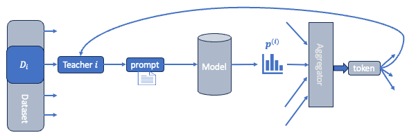
Figure 1: Hot PATE with an auto-regressive base model

Hot PATE (see illustration in Figure 1) partitions $D$ to disjoint parts $D_{i}$ ($i\in[n]$) and constructs a prompt $T_{i}$ from data part $D_{i}$. We then generate a sanitized response sequence $R$ of tokens. We initialize $R\leftarrow\{\}$ and proceed sequentially in lockstep, by repeating the following:

1. For $i\in[n]$: Let $\boldsymbol{p}^{(i)}$ be the output distribution over $V$ when querying the model with the prompt $T_{i}$<instruction to complete prefix>$R$.

2. Apply a DP and diversity-preserving randomized aggregation $\mathcal{M}((\boldsymbol{p}^{(i)})_{i\in[n]})\mapsto y$, where $y\in V$.

3. Concatenate $R\leftarrow R\parallel y$.

This design is open-ended and assumes that the instructions are effective in producing students prompts or components for such prompts, such as representative shots. This assumption aligns with the demonstrated and evolving capabilities of contemporary large language models, as well as the progress made in prompt engineering. An underlying assumption with both cold and hot PATE is that a sufficient number of teachers possess the knowledge we wish to transfer. In both cases the ensemble’s purpose is to privately transfer that knowledge to the student. The key distinction is that with cold PATE, knowledge coverage is achieved by sampling unlabeled examples (or otherwise obtaining representative examples) from the same distribution. These examples are then labeled by the ensemble. In hot PATE, the intent is that coverage is attained organically, through the broad range of diverse responses generated in response to a general instruction within the prompt.

The requirement of preserving diversity, that we will formalize in the sequel, is needed in order to facilitate this knowledge transfer. At a high level, the objective is that the aggregate distribution, the output distribution of $\mathcal{M}((\boldsymbol{p}^{(i)})_{i\in[n]})$, retains the diversity of individual teacher distributions $(\boldsymbol{p}^{(i)})_{i\in[n]}$.

3 Private and diverse aggregation

Diversity and privacy appear to be conflicting in that DP requires that the output token is supported by sufficiently many teachers, a “reporting threshold” that depends on the privacy parameter values. But preserving diversity means that tokens with low probability also need to be transferred to the student.

A natural candidate for preserving diversity is the average teacher distribution $\frac{1}{n}\sum_{i\in[n]}\boldsymbol{p}^{(i)}$. But this is not robust and can not be privacy preserving because tokens that have positive probabilities with only one or few teachers are identifying and should not be released. Fortunately, we can settle for a robust notion of preserving diversity. The premise in PATE is that the patterns of interest are captured by many or even most teachers. Therefore, low probability across many teachers is something we care to transfer whereas high probability in few teachers, the “bad case” for privacy (and robustness), may not be something we have to transfer. The average distribution does not distinguish the two cases, so it is ruled out. We now formalize our nuanced diversity preservation notion:

Definition 1 (Diversity-preserving aggregation of distributions).

Let $f(\boldsymbol{p}^{(i)})_{i\in[n]})\mapsto\boldsymbol{P}$ map from $n$ probability distributions over $V$ to a probability distribution over $V\cup\{\bot\}$. We say that $f$ is diversity-preserving with $\tau\in\mathbbm{N}$, $\beta\in(0,1]$, $\gamma\geq 1$ if for any input and $j\in V$

1. For all $q\in[0,1]$,

   $$(c_{j,q}:=\sum_{i\in n}\mathbbm{1}\{p^{(i)}_{j}\geq q\})\geq\tau\implies P_{j}\geq\beta\cdot\frac{c_{j,q}}{n}q\ .$$

2. $P_{j}\leq\gamma\frac{1}{n}\sum_{i\in[n]}p^{(i)}_{j}$

The first requirement is that probability $q$ across enough ($\tau$) teachers, no matter how small is $q$, is transferred to the aggregate distribution. The second ensures that we do not output irrelevant tokens.

Requirements are stricter (and can be harder to satisfy) when $\beta$ and $\gamma$ are closer to $1$ and when $\tau$ is smaller. A setting of $\tau=0$ and $\beta=\gamma=1$ allows only for the average distribution to be the aggregate. A larger $\tau$ increases robustness in that more teachers must support the transfer.

Remark 1 (failures).

We allow $\bot$ (failure) in the support of the aggregate distribution because under the DP requirement there are input distributions (for example, those with disjoint supports, e.g. responses to instructions that ask for a patient ID) where no token can be returned. Hot PATE has several options to work with failure responses: (i) The step can be repeated (different shared randomness may yield a token), (ii) a response token can instead be sampled from a non-private default prompt or model, or (iii) the prompt instructions can be redesigned.

Remark 2 (Setting of $\tau$).

In homogeneous ensembles, most teachers receive a representative part of the data and possess the knowledge we wish to transfer. This occurs when we use a random partition so that most teachers obtain a representative set of data records. In this case, we aim to transfer the parts of the distributions that are common to most teachers and $\tau>n/2$ suffices. In heterogeneous ensembles, each teacher might have data from one or very few “users.” This arises when each teacher has small capacity (prompts currently have limited size of 8k-64k tokens [Ope23b]) or when by design each teacher is an agent of a single user. In this situation, we aim to transfer parts of the distribution that are common to smaller subgroups of teachers and set $\tau\ll n$, possibly as low as permitted under the privacy requirement.

Before describing DP aggregation methods that satisfy Definition 1, we instructively examine a scheme that can not satisfy the requirements, as it exhibits an inherent privacy-diversity tradeoff: Sample independently $y_{i}\sim\boldsymbol{p}^{(i)}$ for each teacher $i\in[n]$, compute frequencies $c_{j}$ as in (1), and apply any DP aggregation to the histogram $\{(j,c_{j})\}$ (as with cold PATE). Now consider the case of identical teacher distributions that are uniform over $k$ special tokens with probability $q=1/k$ each. From Definition 1, each of the $k$ special tokens needs to be reported with probability at least $\beta/k$. But the frequencies $c_{j}$ of these tokens are concentrated around $c_{j}\approx n/k$. In terms of DP, each frequency value $c_{j}$ has sensitivity $1$ and for large enough $k$, the counts drop below the ”DP reporting threshold” of our privacy parameters and therefore none of these tokens can be reported. To transfer these distributions through such a frequencies histogram we need to adjust the DP parameters to allow for reporting threshold to be below $n/k$, that is, to decrease proportionally to $k$. Therefore, any DP aggregation of this histogram can not satisfy Definition 1 in that it would fail for a sufficiently large $k$. We run into the same issue if we define our histogram with $c_{j}:=\sum_{i}p^{(i)}_{j}$ (as proposed in [DDPB23]). The issue again is that the maximum frequency decreases with diversity ($k$).

The approach where each teacher contributes a sample, however, is appealing as it “factors out” the distributions: Instead of aggregating distributions, we work with a histogram of frequencies. But with independent sampling we arrived at a dead end – and it may seem that we need to ditch the sampling approach all together. Fortunately, our proposed aggregation method also samples teacher distributions to generate a histogram of frequencies. The difference is that the frequency of a token is not concentrated around its expectation. A tokens $j$ that broadly has a low probability $q$ will appear, sometimes, with very high frequency $c_{j}$ that does not depend on $q$. What does depend on $q$ is the probability of this event. This allows it to pass through a high “privacy threshold.”

4 Ensemble coordination

Ensemble coordination, described in Algorithm 1, is a randomized mapping from a set of $n$ probability distributions over $V$ to a histogram over $V$ with total count $n$. We sample shared randomness $\rho$. For each teacher $i\in[n]$ we compute $y_{i}\in V$ that is a function of $\rho$ and $\boldsymbol{p}^{(i)}$. We then compute the frequencies $c_{j}$ for $j\in V$, as in (1), and return the frequency histogram.

Input: Teacher distributions $(\boldsymbol{p}^{(i)})_{i\in[n]}$

foreach token $j\in V$ do draw iid $u_{j}\sim\mathsf{Exp}[1]$

  // Draw shared randomness $\rho=(u_{j})_{j\in V}$ foreach teacher $i$ do // Draw coordinated samples $(y_{i})_{i\in[n]}$

      $y_{i}\leftarrow\arg\max_{j}\frac{p^{(i)}_{j}}{u_{j}}$

        // bottom-$k$ sampling transform

      

foreach token $j\in V$ do // Compute frequencies

      $c_{j}\leftarrow\sum_{i\in[n]}\mathbbm{1}\{y_{i}=j\}$

return $\{(j,c_{j})\}_{j\in V}$, $\rho=(u_{j})_{j}$// Histogram of frequencies

Algorithm 1 CoordinatedSamples

Importantly, ensemble coordination over prompts can be implemented via an enhanced API access to the model. The best approach is to support the shared randomness $\rho$ as input along with the query. Alternatively, we can use API access that returns the distribution over tokens – The current OpenAI text completion interface returns the five highest probabilities [Ope23b].

The sampling method in ensemble coordination is a classic technique called coordinated sampling. The technique was first introduced in statistics applications in order to obtain samples that are stable under distribution shifts [KS71, BEJ72, Saa95, Ros97, Ohl00]. It was then introduced in computer science for sampling-based sketches and a form of Locality Sensitive Hashing (LSH) [Coh94, Coh97, Bro00, IM98].

Similarly to independent sampling, the marginal distribution of $y_{i}$ for each teacher $i$ is simply $\boldsymbol{p}^{(i)}$. Therefore, the expected frequency of token $j$ is

$$\mathsf{E}_{\rho}[c_{j}]=\sum_{i}p^{(i)}_{j}\ .$$ (2)

The key difference is that votes of different teachers are highly positively correlated. For two teacher distributions $i,k$, the probability of them having the same sample is the weighted Jaccard similarity of the distributions:

$$\Pr_{\rho}[y_{i}=y_{k}]=\frac{\sum_{j}\min\{p^{(i)}_{j},p^{(k)}_{j}\}}{\sum_{j}\max\{p^{(i)}_{j},p^{(k)}_{j}\}}$$

In particular, when two distributions are identical, the samples are the same $y_{i}=y_{k}$.

We establish that the respective requirements of Definition 1, diversity-transfer and relevance, can be satisfied by only selecting tokens that appear with high frequency in the histogram. We show that a token $j$ for which $m$ teachers $i$ have $p^{(i)}_{j}>q$ has frequency at least $m/2$ with probability at least $0.34q$ (see proof in Appendix C):

Lemma 1 (diversity transfer).

For any token $j$ and $p,q\in[0,1]$,

$$\Pr_{\rho}\left[c_{j}\geq p\cdot\sum_{i\in n}\mathbbm{1}\{p^{(i)}_{j}\geq q\}\right]\geq\frac{1}{2}\ln(1/p)q$$

To establish relevance we show that high frequency must have a “backing.” The following is immediate from (2) and Markov’s inequality (and is tight in the sense that for any $T$ there are distributions where equality holds):

Lemma 2 (relevance).

For any token $j$ and $T$,

$$\Pr_{\rho}\left[c_{j}\geq T\right]\leq\frac{1}{T}\sum_{i\in[n]}p^{(i)}_{j}$$

Therefore, broadly speaking, it is possible to satisfy the requirements of Definition 1 by reporting only tokens with frequency that is $\Omega(\tau)$, where $\tau$ is the required teachers support. Our DP aggregation methods are presented in Section 6.

5 Empirical demonstration

We demonstrate the properties of coordinated ensembles using the OpenAI GPT3.5 text completion interface [Ope23b]. Given a text prompt, the interface provides the tokens and probabilities of the top-5 tokens. We generated $10^{3}$ queries (prompts) of the following form (see Example in Figure 2) and collected the top-5 tokens and their probabilities.

On planet Z, some numbers are edible. <name> from planet Z eats the following numbers for breakfast: <random permutation of $\{63,56,28,17\}\cup\{m\sim U\{11,\ldots,99\}$> Give me an example breakfast number in planet Z. Respond with just the number.

The top 5 tokens returned in all of the $10^{3}$ queries were 2 digit decimal numbers. The response token was more likely to be one of the example numbers in the prompt than a different number.

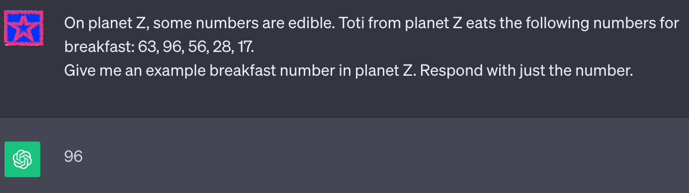
Figure 2: Query to GPT3.5

Our queries were constructed to have a shared “general” component that we aim to capture via the private aggregation: The four common numbers that we color-code in plots $17$,$28$,$56$, $63$. Other components such as the name and the fifth number are considered “private.” A limitation of the interface is that we can not obtain the full distribution over tokens. We thus scaled up each partial distribution of top-5 to obtain a distribution $\boldsymbol{p}^{(i)}$ for queries $i\in[10^{3}]$.

Figure 3 (left) reports the distribution of the average probabilities $10^{-3}\sum_{i=1}^{10^{3}}\boldsymbol{p}^{(i)}$ of each token with a positive probability. The model displayed some preference for $63$ over the three other special numbers. The right plot is a histogram of the frequencies (normalized by $10^{3}$) obtained by independently sampling one token $y_{i}$ from each distribution $\boldsymbol{p}^{(i)}$. There was little notable change between different sampling: For each token $j$, the frequency is a sum of independent Poisson random variables with parameters $p^{(i)}_{j}$, that we know from standard tail bounds to be concentrated around its expectation.

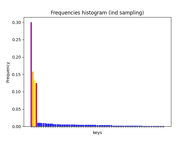
Figure 3: Average probabilities (left) and normalized frequency histogram from independent samples (right)

Figure 4 reports example frequency histograms obtained with coordinated sampling (Algorithm 1) for three samples of the shared randomness $\rho$. Note that a different special token dominates each histogram, and the maximum frequency is much higher than the respective expected value.

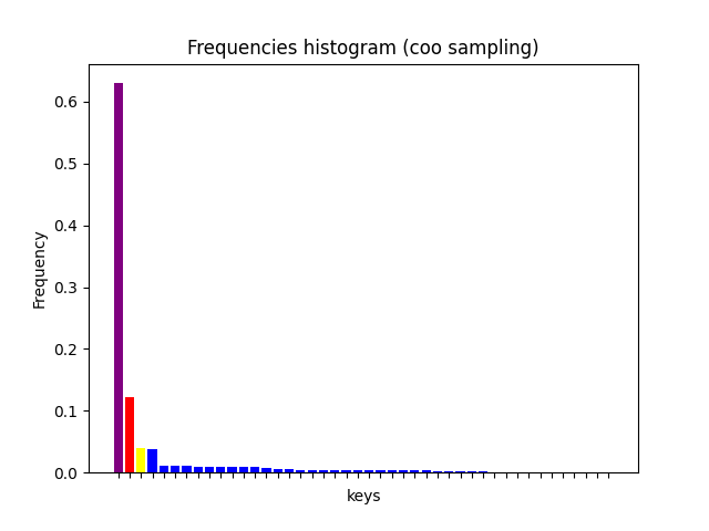
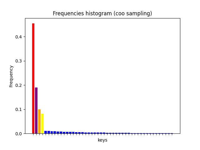
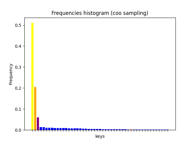
Figure 4: Histograms from coordinated samples for different sampling of shared randomness $\rho$

Figure 5 reports aggregate results for $10^{3}$ frequency histograms produced for each of coordinated and independent samples. From each histogram we collected the highest and second highest frequencies of a special number and the highest frequency of a non-special number. The left plot shows the counts (sorted in decreasing order) of each of these three values. Note that with independent samples, frequencies remain close to their expectations: The top frequency corresponds to that of $63$. The second highest to one of the other special numbers. Note that with independent sampling no token (special or not) in no trial had frequency $>0.5$. Moreover, the gap between the top and second frequencies was consistent and reflected the gap of the expected frequencies between the two top special tokens.

With coordinated samples, about half of the trials had a dominant token with frequency $>0.5$. The dominant token was always one of the special tokens, but not necessarily the special token with the highest average frequency. Figure 5 (right) shows the probability of each of the special numbers to have frequency above $>0.5$. We can see that all four special numbers are represented with probability roughly proportional to their average probability.

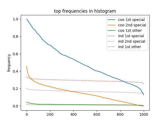
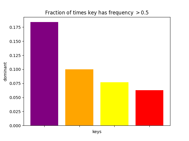
Figure 5: Counts of top frequencies in decreasing order (left). Distribution of dominant token (right)

We observe two benefits of coordinated sampling. First, tokens appear with high frequency, which is easier to report privately. Second, when there is dominance, there tends to be a large gap between the highest and second highest frequencies, which is beneficial with data-dependent privacy analysis.

Due to the limitation of the interface that returns only the top 5 probabilities, we constructed our example to have $k=4$ special tokens that should be transferred to the student distribution. Note that the benefits of coordinated sampling scale up with $k$: With $k$ special tokens, the top frequency with independent sampling decreases proportionally to $k$ whereas the top frequency with coordinated sampling remains high and does not depend on $k$. With larger $k$, the lines for coordinated sampling in Figure 5 (left) would remain the same whereas the lines for independent sampling would shift down proportionally to $k$. This point follows from the analysis and is demonstrated via simulations in Section A.

6 Aggregation Methods of Frequency Histograms

Our aggregation methods are applied to frequency histograms generated by a coordinated ensemble and return a token or $\bot$. We propose two meta schemes that preserves diversity in the sense of Definition 1: One for homogeneous ensembles, where we use $\tau>n/2$, in Section 6.1 and one for heterogeneous ensembles, where $\tau\ll n/2$ (but large enough to allow for DP aggregation), in Section 6.2. To establish diversity preservation, we consider the end-to-end process from the teacher distributions to the aggregate distribution. To establish privacy, it suffices to consider the histogram in isolation, as it has the same sensitivity as vote histograms with cold PATE: When one teacher distribution changes, one token can gain a vote and one token can lose a vote. This because the shared randomness $\rho$ is considered “public” data. We then explore (Sections A and B) DP implementations that admit data-dependent privacy analysis so effectively many more queries can be performed for the same privacy budget. The latter benefits from the particular structure of histograms generated by coordinated ensembles. The privacy loss does not depend on queries with no yield, with high agreement, or with agreement with a public prior. With heterogeneous ensembles we can also gain from individualized per-teacher privacy charging.

6.1 Homogeneous Ensembles

$\boldsymbol{c},\rho\leftarrow\textnormal{{CoordinatedSamples}}((\boldsymbol{p}^{(i)})_{i\in[n]})$

  // Algorithm 1

$(j,\hat{c}_{j})\leftarrow\texttt{NoisyArgMax}_{L}(\boldsymbol{c})$

  // DP noisy maximizer with error $L$

if $\hat{c}_{j}>(n/2+L)$ then return $j$ else return $\bot$

 

Algorithm 2 DistAgg homogeneous

When $\tau>n/2$, there can be at most one token $j$ with frequency $c_{j}\geq\tau$. If there is such a token, we aim to report it. Otherwise, we return $\bot$. Our scheme is described in Algorithm 2 in terms of a noisy maximizer (NoisyArgMax_L) procedure. The latter is a well studied construct in differential privacy [MT07, DR19, QSZ21]. Generally, methods vary with the choice of noise distribution and there is a (high probability) additive error bound $L$ that depends on the privacy parameters and in some cases also on the support size and confidence. For our purposes, we abstract this as NoisyArgMax_L that is applied to a frequency histogram $\boldsymbol{c}$ and returns $(j,\hat{c}_{j})$ such that $|c_{j}-\hat{c}_{j}|<L$ and $\max_{h\in V}c_{h}-c_{j}\leq 2L$. We show that the method is diversity preserving (proof is provided in Appendix C):

Lemma 3 (Diversity-preservation of Algorithm 2).

For $\mu>1$, Algorithm 2, instantiated with NoisyArgMax_L as described, is diversity preserving in the sense of Definition 1 with $\tau=\mu(n/2+2L)$, $\beta=\ln(\mu)/2$ and $\gamma=2$.

The two most common noise distributions for DP are Gaussian and Laplace noise. (Cold) PATE was studied with both. The Gaussian-noise based Confident-GNMax aggregator [PSM⁺18, DDPB23] empirically outperformed the Laplace-based LNMAX [PAE⁺17] on cold PATE. for Algorithm 2. The advantages of Gaussian noise are concentration (less noise to separate a maximizer from low frequency tokens), efficient composition, and more effective data dependent privacy analysis. Laplace-based noise on the other hand can preserve sparsity (a consideration as the key space of tokens or strings of token can be quite large), there is an optimized mechanism with sampling (for medium agreement), and there are recent improvement on data-dependent privacy analysis across many queries (the situation with hot PATE) [CL23]. Our privacy analysis in Section A uses a data-dependent Laplace-based approach.

6.2 Heterogeneous Ensembles

$\boldsymbol{c},\rho\leftarrow\textnormal{{CoordinatedSamples}}((\boldsymbol{p}^{(i)})_{i\in[n]})$

  // Algorithm 1

Sample $j\in V$ with probability $\frac{c_{j}}{n}$

  // Weighted sampling of a token from $\boldsymbol{c}$

if $c_{j}\geq 2L$ then return $j$ else return $j$ or $\bot$

 

Algorithm 3 DistAgg Heterogeneous

For lower values of $\tau$, we propose the meta-scheme described in Algorithm 3: We perform weighted sampling of a token from $\boldsymbol{c}$ and return it if its count exceeds $2L$. If it is below $2L$ we may return either $j$ or $\bot$. We propose DP implementations in Section B. We establish that Algorithm 3 is diversity-preserving (proof provided in Appendix C).

Lemma 4 (Diversity-preservation of Algorithm 3).

For $\mu>1$, Algorithm 3 is diversity preserving in the sense of Definition 1 with $\tau=\mu 2L$, $\beta=\frac{1}{2\mu}\ln(\mu)$ and $\gamma=1$.

Conclusion

We proposed and evaluated hot PATE, an extension of the PATE framework that facilitates open ended private learning via prompts. The design is based on a notion of a robust and diversity-preserving aggregation of distributions with methods to implement it in a privacy-preserving way.

We expect our design to find further applications beyond the PATE setting. The framework is applicable generally when users contribute distributions (that may reflect their preferences) that are private information and the goal is to obtain a public representative bundle of items. Moreover, our notion of robust aggregate distributions may be useful in applications that require robustness but not necessarily privacy. In a sense, it complements a different aggregate distribution, the multi-objective sampling distribution [Coh15], where the goal is to faithfully capture each input distribution with minimum overhead.

Appendix A Privacy analysis considerations

The effectiveness of Hot PATE depends on the number of queries with yield (token returned) that can be returned for a given privacy budget. We explore the benefits of data-dependent privacy analysis when the aggregation follows Algorithm 2 (homogeneous ensembles). Broadly speaking, with data-dependent analysis, we incur higher privacy loss on “borderline” queries where the output of the DP aggregation has two or more likely outputs. Queries that return a particular token with high probability or return $\bot$ with high probability incur little privacy loss. This means generally that we can process many more queries for the privacy budget than if we had just used a DP composition bound.

We demonstrate that with Algorithm 2, we can expect that only a small fraction of frequency histograms generated by coordinated ensembles are “borderline.” (i) For queries with high yield (high probability of returning a token over the sampling of the shared randomness), the generated histograms tend to have a dominant token (and thus lower privacy loss). This because coordinated ensembles tend to “break ties” between tokens. (ii) For queries with low yield (high probability of $\bot$ response and low probability of returning a token), the total privacy loss only depends on yield responses. This means that high $\bot$ probability does not cause performance to deteriorate.

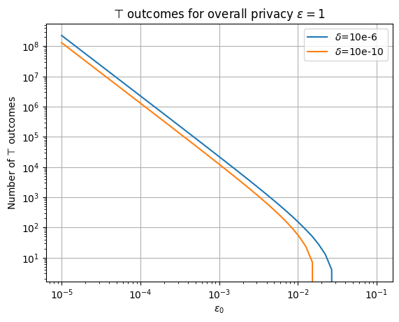
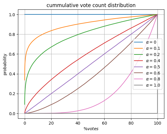
Figure 6: Left: Number of $\top$ responses for $\varepsilon_{0}$-DP queries for total $\varepsilon=1$ loss. Right: Cummulative maximum frequency for varying common part $\alpha$.

Concretely we consider NoisyArgMax using [CGSS21]  with the maximum sanitized frequency, with privacy parameters $(\varepsilon_{0},\delta_{0})$. For privacy analysis across queries we applied the Target Charging Technique (TCT) of [CL23] with the boundary-wrapper method. The wrapper modifies slightly the output distribution of the query algorithm (after conditioning on $\rho$!) to include an additional outcome $\top$ (target). The wrapper returns $\top$ with this probability (that depends on the response distribution) and otherwise returns a sample from the output distribution of the wrapped algorithm. The probability of $\top$ is at most $1/3$ and decreases with agreement (vanishes when there is response with probability closer to $1$). The technique allows us to analyse the privacy loss by only counting target hits, that is, queries with $\top$ response. Since the probability of $\top$ is at most $1/3$, we get in expectation at least two useful responses per target hit. But in case of agreements, we can get many more. Figure 6 (left) reports the number of $\top$ (target) responses we can have with the boundary wrapper method as a function of $\varepsilon_{0}$ with overall privacy budget is $\varepsilon=1$. When $\varepsilon_{0}\leq 0.01$, it is about $(10\varepsilon_{0})^{-2}$.

With hot PATE, we are interested in yield responses, those that return a token (not $\bot$, and when we apply the boundary wrapper, also not $\top$). We study how the yield probability behaves for histograms generated by coordinated ensembles. We parametrize the set of teacher distributions by $\alpha\in(0,1]$, which is the probability of a common part to all distribution and what we aim to transfer to the student. Our teacher distributions have probability vectors of the form $\boldsymbol{p}^{(i)}=\alpha\cdot\boldsymbol{s}+(1-\alpha)\cdot\boldsymbol{r}^{(i)}$, where $\boldsymbol{s}$ and $\boldsymbol{r}^{(i)}$ are probability vectors. That is, with probability $\alpha$ there is a sample from the common distribution $\boldsymbol{s}$, and with probability $(1-\alpha)$, there is a sample from an arbitrary distribution. When the histogram is generated by a coordinated ensemble, then the distribution of the maximum frequency $c$ of a token is dominated by sampling $y\sim\mathsf{Exp}[\alpha]$ and then $c\sim\mathsf{Bin}[e^{-y\cdot(1-\alpha)},n]$. It is visualized in Figure 6 (right) for varying values of $\alpha$. Note that across all $\alpha>0$, no matter how small $\alpha$ is, there is probability $\approx\alpha$ of being above a high threshold (and returning a token). The probability of $\bot$ (no agreement) in this case can be $\approx 1-\alpha$. Therefore $\alpha$ parametrizes the probability of yield over the sampling of the shared randomness.

Figure 7: Sweep of $\alpha$, showing probabilities of outcomes: token, $\bot$, $\top$ (target hit).

Figure 7 shows the distribution of responses as we sweep $\alpha$, broken down by $\top$ (target hit), $\bot$ (abort), and token (yield). The number of queries we process per target hit, which is the inverse of the probability of $\top$, is $\gtrapprox\varepsilon_{0}n$. It is lowest at $\alpha\approx T/n$ and is very high for small and large $\alpha$, meaning that the privacy cost per query is very small.

The yield (probability of returning a token) per query is $\approx\alpha$. Note that as $\alpha$ decreases, both yield and target probabilities decrease but their ratio remains the same: In the regime $\alpha\leq T/n$, the yield per target hit is $\approx\varepsilon_{0}n/2$. Queries with $\alpha\gg T/n$ are essentially free in that the yield (token) probability is very high and the $\top$ (target hit) probability is very low.

When using $n=C_{\delta}/\varepsilon_{0}$ ($C_{\delta}\approx 2\log(1/\delta_{0}$) teachers and plugging this in, we obtain that we get $\gtrapprox 0.005\frac{1}{C_{\delta}}n^{2}$ yields for overall privacy budget $\varepsilon=1$. This means that we pay only for yield and not for queries. Note that this holds in the “worst case” across all $\alpha$ values, but the number of yields can be much higher when queries have large $\alpha$ (and “yields” do not incur privacy loss).

Appendix B DP methods for heterogeneous ensembles

We propose two DP methods to implement Algorithm 3 (Section 6.2) with different trade offs. In both cases we can apply data-dependent privacy analysis so that queries that do not yield a token (that is, return $\bot$) are essentially “free” in terms of the privacy loss. The parameter $L$ depends on the privacy parameters (and logarithmically on $|V|$).

Importantly however, with the second method we can apply privacy analysis with individual charging, where instead of charging the whole ensemble as a unit we only charge teachers that contributed to a response. With heterogeneous ensembles we expect the diversity to arise both from individual distributions and from differences between teachers and therefore with individual charging allows for much more efficient privacy analysis when different groups of teachers support each prediction.

Private Weighted Sampling

This method gains from sparsity (histogram support being much smaller than $|V|$) but the calculation of privacy loss is for the whole ensemble. We can do the analysis in the TCT framework [CL23] so that privacy loss only depends on yield queries (those that return a token). We perform weighted sampling by frequency of each token to obtain the sampled histogram $\boldsymbol{c}^{\prime}$ and then sanitize the frequencies of sampled tokens using the end-to-end sparsity-preserving method of [CGSS21] to obtain $\boldsymbol{c}^{*}$. The sanitizing prunes out some tokens from $\boldsymbol{c}^{\prime}$ with probability that depends on the frequency $c_{j}$, privacy parameters, and sampling rate. All tokens in $\boldsymbol{c}^{\prime}$ with frequency above $2L$, where $L$ only depends on the privacy parameters, remain in $\boldsymbol{c}^{*}$. The final step is to return a token from $\boldsymbol{c}^{*}$ selected uniformly at random or to return $\bot$ if $\boldsymbol{c}^{*}$ is empty.

Individual Privacy Charging

This method does not exploit sparsity, but benefits from individual privacy charging [KMS21, CL23]. It is appropriate when $2L\ll n$. The queries are formulated as counting queries over the set of teachers. The algorithm maintain a per-teacher count of the number of counting queries it “impacted.” A teacher is removed from the ensemble when this limit is reached. Our queries are formed such that at most $O(2L)$ teachers (instead of the whole ensemble) can get “charged” for each query that yields a token.

To express Algorithm 3 via counting queries we do as follows: We draw a sampling rate of teachers uniformly from $1/n,\ldots,1$ and then uniformly draw a token from $v\in V$. We sample the teachers with this sampling rate and count the number $c^{\prime}_{v}$ of sampled teachers with $y_{i}=v$. We then do a BetweenThresholds test on $c^{\prime}_{j}$ (using [CL23] which improves over [BSU17]) to check if $c^{\prime}_{v}\geq 2L$. For “above” or “between” outcomes we report $v$. If it is a “between” outcome we increment the loss counter of all sampled teachers with $y_{i}=v$ (about $2L$ of them). We note that this process can be implemented efficiently and does not require explicitly performing this “blind” search.

Teachers that reach their charge limit get removed from the ensemble. The uniform sampling of the sampling rate and token emulates weighted sampling, where the probability that a token gets selected is proportional to its frequency. The sub-sampling of teachers ensures that we only charge the sampled teachers. Teachers are charged only when the query is at the “between” regime so (with high probability) at most $\approx 2L$ teachers are charged. Because we don’t benefit from sparsity, there is overhead factor of $\log(|V|(n/L))$ in the privacy parameter (to bound the error of this number of queries) but we gain a factor of $n/L$ by not charging the full ensemble for each query in the heterogeneous case where most teachers have different “solutions” to contribute.

Appendix C Proofs

Proof of Lemma 1.

Let $i$ be such that $p^{(i)}_{j}\geq q$. Fix the sampled min value $x\sim\mathsf{Exp}[q]$ for $q$ part of the probability of $j$. We get that

$$\Pr[y_{i}=j] \geq\Pr_{y\sim\mathsf{Exp}[1-q]}[y>x]=e^{-x(1-q)}$$

For $x<\frac{-\ln p}{1-q}$ we have that the probability is at least $e^{-x(1-q)}\geq p$. Different teachers that share part of the distribution can only be positive ly correlated. So we get that if there are $c_{j,q}$ teachers with $p^{(i)}_{j}\geq q$ then the distribution of the number of teachers with $y_{i}=j$ dominates $\mathsf{Bin}[e^{-x(1-q)},c_{j,q}]$, which for any $x\leq\frac{-\ln p}{1-q}$ dominates $\mathsf{Bin}[p,c_{j,q}]$. So with probability at least $1/2$, we have at least $pc_{j,q}$ teachers with $y_{i}=j$.

This happens with probability at least

$$\Pr_{x\sim\mathsf{Exp}[q]}[x<\frac{-\ln p}{1-q}]=1-e^{(\ln p)q/(1-q)}\geq-(\ln p)q$$

For $p=1/2$ we get that the probability is $\geq 0.69q$. For $p=2/3$ it is $\geq 0.4q$.

∎

Proof of Lemma 3.

We apply Lemma 1 with $p=1/\mu$. We obtain that the token $j$ has frequency at least $c_{j}\geq n/2+2L$ with probability at least $0.5\ln(\mu)q$. Therefore we have $\hat{c}_{j}\geq n/2+L$ with probability at least $0.5\ln(\mu)q$. Note that a token can only be reported if its frequency is $c_{j}>n/2$. Using $T=n/2$ in Lemma 2 we obtain that the relevance requirement is satisfied with $\gamma=2$. ∎

Proof of Lemma 4.

Consider the first requirement of Definition 1. Consider a token $j$ with $c_{j,q}\geq\tau$. From Lemma 1 using $p=1/\mu$ we obtain that the token $j$ has frequency at least $c_{j}\geq c_{j,q}/\mu\geq 2L$ with probability at least $0.5\ln(\mu)q$. The token is sampled with probability $\min\{1,kc_{j}/n\}$ and if so appears also in $\boldsymbol{c}^{*}$ (since $c_{j}\geq 2L$). The expected size (number of entries) of $\boldsymbol{c}^{*}$ is at most $k$ and thus it is returned if sampled with probability at least $1/k$. Overall it is sampled and reported with probability at least $\min\{1/k,c_{j}/n\}$. In total, the probability is $P_{j}\geq\min\{1/k,c_{j,q}/(\mu n)\}0.5\ln(\mu)q\geq\frac{1}{2k\mu}\ln(\mu)\frac{c_{j,q}}{n}q$.

The second requirement of Definition 1 is immediate. The expected frequency of token $j$ is $\sum_{i\in[n]}p^{(i)}_{j}$ and it is sampled with probability at most $\frac{k}{n}\sum_{i\in[n]}p^{(i)}_{j}$. It can only be the output if sampled. ∎

References

- [ACG+16] Martín Abadi, Andy Chu, Ian J. Goodfellow, H. Brendan McMahan, Ilya Mironov, Kunal Talwar, and Li Zhang. Deep learning with differential privacy. In Edgar R. Weippl, Stefan Katzenbeisser, Christopher Kruegel, Andrew C. Myers, and Shai Halevi, editors, Proceedings of the 2016 ACM SIGSAC Conference on Computer and Communications Security, Vienna, Austria, October 24-28, 2016. ACM, 2016.
- [BEJ72] K. R. W. Brewer, L. J. Early, and S. F. Joyce. Selecting several samples from a single population. Australian Journal of Statistics, 14(3):231–239, 1972.
- [BMR+20] Tom B. Brown, Benjamin Mann, Nick Ryder, Melanie Subbiah, Jared Kaplan, Prafulla Dhariwal, Arvind Neelakantan, Pranav Shyam, Girish Sastry, Amanda Askell, Sandhini Agarwal, Ariel Herbert-Voss, Gretchen Krueger, Tom Henighan, Rewon Child, Aditya Ramesh, Daniel M. Ziegler, Jeffrey Wu, Clemens Winter, Christopher Hesse, Mark Chen, Eric Sigler, Mateusz Litwin, Scott Gray, Benjamin Chess, Jack Clark, Christopher Berner, Sam McCandlish, Alec Radford, Ilya Sutskever, and Dario Amodei. Language models are few-shot learners, 2020.
- [BNS19] Mark Bun, Kobbi Nissim, and Uri Stemmer. Simultaneous private learning of multiple concepts. J. Mach. Learn. Res., 20:94:1–94:34, 2019.
- [Bro00] A. Z. Broder. Identifying and filtering near-duplicate documents. In Proc.of the 11th Annual Symposium on Combinatorial Pattern Matching, volume 1848 of LNCS, pages 1–10. Springer, 2000.
- [BSU17] Mark Bun, Thomas Steinke, and Jonathan Ullman. Make Up Your Mind: The Price of Online Queries in Differential Privacy, pages 1306–1325. 2017.
- [BTGT18] Raef Bassily, Om Thakkar, and Abhradeep Guha Thakurta. Model-agnostic private learning. In S. Bengio, H. Wallach, H. Larochelle, K. Grauman, N. Cesa-Bianchi, and R. Garnett, editors, Advances in Neural Information Processing Systems, volume 31. Curran Associates, Inc., 2018.
- [CGSS21] Edith Cohen, Ofir Geri, Tamas Sarlos, and Uri Stemmer. Differentially private weighted sampling. In Proceedings of The 24th International Conference on Artificial Intelligence and Statistics, volume 130 of Proceedings of Machine Learning Research. PMLR, 2021.
- [CL23] Edith Cohen and Xin Lyu. The target-charging technique for privacy accounting across interactive computations. CoRR, abs/2302.11044, 2023.
- [Coh94] E. Cohen. Estimating the size of the transitive closure in linear time. In Proc. 35th IEEE Annual Symposium on Foundations of Computer Science, pages 190–200. IEEE, 1994.
- [Coh97] E. Cohen. Size-estimation framework with applications to transitive closure and reachability. J. Comput. System Sci., 55:441–453, 1997.
- [Coh15] E. Cohen. Multi-objective weighted sampling. In HotWeb. IEEE, 2015. full version: http://arxiv.org/abs/1509.07445.
- [DDPB23] Haonan Duan, Adam Dziedzic, Nicolas Papernot, and Franziska Boenisch. Flocks of stochastic parrots: Differentially private prompt learning for large language models, 2023.
- [DMNS06] Cynthia Dwork, Frank McSherry, Kobbi Nissim, and Adam Smith. Calibrating noise to sensitivity in private data analysis. In TCC, 2006.
- [DR14] Cynthia Dwork and Aaron Roth. The algorithmic foundations of differential privacy. Foundations and Trends in Theoretical Computer Science, 9(3–4):211–407, 2014.
- [DR19] David Durfee and Ryan M. Rogers. Practical differentially private top-k selection with pay-what-you-get composition. In Hanna M. Wallach, Hugo Larochelle, Alina Beygelzimer, Florence d’Alché-Buc, Emily B. Fox, and Roman Garnett, editors, Advances in Neural Information Processing Systems 32: Annual Conference on Neural Information Processing Systems 2019, NeurIPS 2019, December 8-14, 2019, Vancouver, BC, Canada, pages 3527–3537, 2019.
- [GRS12] Arpita Ghosh, Tim Roughgarden, and Mukund Sundararajan. Universally utility-maximizing privacy mechanisms. SIAM J. Comput., 41(6):1673–1693, 2012.
- [GTLV23] Shivam Garg, Dimitris Tsipras, Percy Liang, and Gregory Valiant. What can transformers learn in-context? a case study of simple function classes, 2023.
- [IM98] P. Indyk and R. Motwani. Approximate nearest neighbors: Towards removing the curse of dimensionality. In Proc. 30th Annual ACM Symposium on Theory of Computing, pages 604–613. ACM, 1998.
- [JYvdS18] James Jordon, Jinsung Yoon, and Mihaela van der Schaar. Pate-gan: Generating synthetic data with differential privacy guarantees. In International Conference on Learning Representations, 2018.
- [KKMN09] Aleksandra Korolova, Krishnaram Kenthapadi, Nina Mishra, and Alexandros Ntoulas. Releasing search queries and clicks privately. In Juan Quemada, Gonzalo León, Yoëlle S. Maarek, and Wolfgang Nejdl, editors, Proceedings of the 18th International Conference on World Wide Web, WWW 2009, Madrid, Spain, April 20-24, 2009, pages 171–180. ACM, 2009.
- [KMS21] Haim Kaplan, Yishay Mansour, and Uri Stemmer. The sparse vector technique, revisited. In Mikhail Belkin and Samory Kpotufe, editors, Conference on Learning Theory, COLT 2021, 15-19 August 2021, Boulder, Colorado, USA, volume 134 of Proceedings of Machine Learning Research, pages 2747–2776. PMLR, 2021.
- [KS71] L. Kish and A. Scott. Retaining units after changing strata and probabilities. Journal of the American Statistical Association, 66(335):pp. 461–470, 1971.
- [LSZ+21] Jiachang Liu, Dinghan Shen, Yizhe Zhang, Bill Dolan, Lawrence Carin, and Weizhu Chen. What makes good in-context examples for gpt-3? CoRR, abs/2101.06804, 2021.
- [LWY+21] Yunhui Long, Boxin Wang, Zhuolin Yang, Bhavya Kailkhura, Aston Zhang, Carl Gunter, and Bo Li. G-pate: Scalable differentially private data generator via private aggregation of teacher discriminators. In M. Ranzato, A. Beygelzimer, Y. Dauphin, P.S. Liang, and J. Wortman Vaughan, editors, Advances in Neural Information Processing Systems, volume 34, pages 2965–2977. Curran Associates, Inc., 2021.
- [MT07] Frank McSherry and Kunal Talwar. Mechanism design via differential privacy. In 48th Annual IEEE Symposium on Foundations of Computer Science (FOCS 2007), October 20-23, 2007, Providence, RI, USA, Proceedings, pages 94–103. IEEE Computer Society, 2007.
- [NRS07] Kobbi Nissim, Sofya Raskhodnikova, and Adam Smith. Smooth sensitivity and sampling in private data analysis. In Proceedings of the thirty-ninth annual ACM symposium on Theory of computing, pages 75–84, 2007.
- [Ohl00] E. Ohlsson. Coordination of pps samples over time. In The 2nd International Conference on Establishment Surveys, pages 255–264. American Statistical Association, 2000.
- [Ope23a] OpenAI. OpenAI pricing for language models, 2023.
- [Ope23b] OpenAI. OpenAI text completion API documentation, 2023.
- [PAE+17] Nicolas Papernot, Martín Abadi, Úlfar Erlingsson, Ian J. Goodfellow, and Kunal Talwar. Semi-supervised knowledge transfer for deep learning from private training data. In 5th International Conference on Learning Representations, ICLR 2017, Toulon, France, April 24-26, 2017, Conference Track Proceedings. OpenReview.net, 2017.
- [PSM+18] Nicolas Papernot, Shuang Song, Ilya Mironov, Ananth Raghunathan, Kunal Talwar, and Úlfar Erlingsson. Scalable private learning with PATE. In 6th International Conference on Learning Representations, ICLR 2018, Vancouver, BC, Canada, April 30 - May 3, 2018, Conference Track Proceedings. OpenReview.net, 2018.
- [QSZ21] Gang Qiao, Weijie J. Su, and Li Zhang. Oneshot differentially private top-k selection. In Marina Meila and Tong Zhang, editors, Proceedings of the 38th International Conference on Machine Learning, ICML 2021, 18-24 July 2021, Virtual Event, volume 139 of Proceedings of Machine Learning Research, pages 8672–8681. PMLR, 2021.
- [Ros97] B. Rosén. Asymptotic theory for order sampling. J. Statistical Planning and Inference, 62(2):135–158, 1997.
- [RWC+19] Alec Radford, Jeff Wu, Rewon Child, David Luan, Dario Amodei, and Ilya Sutskever. Language models are unsupervised multitask learners. 2019.
- [Saa95] P. J. Saavedra. Fixed sample size pps approximations with a permanent random number. In Proc. of the Section on Survey Research Methods, pages 697–700, Alexandria, VA, 1995. American Statistical Association.
- [Vad17] Salil Vadhan. The Complexity of Differential Privacy. 04 2017.
- [YNB+22] Da Yu, Saurabh Naik, Arturs Backurs, Sivakanth Gopi, Huseyin A. Inan, Gautam Kamath, Janardhan Kulkarni, Yin Tat Lee, Andre Manoel, Lukas Wutschitz, Sergey Yekhanin, and Huishuai Zhang. Differentially private fine-tuning of language models. In The Tenth International Conference on Learning Representations, ICLR 2022, Virtual Event, April 25-29, 2022. OpenReview.net, 2022.
- [ZNL+22] Hattie Zhou, Azade Nova, Hugo Larochelle, Aaron Courville, Behnam Neyshabur, and Hanie Sedghi. Teaching algorithmic reasoning via in-context learning, 2022.