Department of Physics, Indian Institute of Technology - Kanpur,
Kanpur 208016, India

We compute tree level scattering amplitudes involving more than one highly excited states and tachyons in bosonic string theory. We use these amplitudes to understand chaotic and thermal aspects of the excited string states lending support to the Susskind-Horowitz-Polchinski correspondence principle. The unaveraged amplitudes exhibit chaos in the resonance distribution as a function of kinematic parameters, which can be described by random matrix theory. Upon coarse-graining these amplitudes are shown to exponentiate, and capture various thermal features, including features of a stringy version of the eigenstate thermalization hypothesis as well as notions of typicality. Further, we compute the effective string form factor corresponding to the highly excited states, and argue for the random walk behaviour of the long strings.

1 Context

Black holes are chaotic and thermal quantum objects. Both these notions have by now been well established classically. For instance, it has been known since long that classical orbits around Schwarzchild black holes exhibit chaos [1]. The quantum origins of these phenomena is an area of active research, with connections being recently made between black holes and quantum chaos in [2, 3, 4, 5]. The horizon plays an important role in these computations which gives rise to exponential red-shift. The quantum effects of horizon physics can be traced back to Hawking’s calculation of black hole radiation [6] which points towards a thermal interpretation. This has since then created the information loss enigma. In a full quantum gravity theory, this problem can be cast as a feature of the theory, known as the central dogma [7] : which states that the black hole as seen by an exterior observer is described by a unitary theory with $A/4G$ quantum degrees of freedom. A strong evidence for the dogma comes from reproduction of the Bekenstein-Hawking black hole entropy formula for special extremal black holes in supersymmetric string theories [8, 9]. This counting is possible in the string theory’s weak coupling limit due to enough supersymmetry. A primer to these computations in the context of black holes in string theory appear through the correspondence principle.

The Susskind-Horowitz-Polchinski correspondence principle [10, 11] conjectures that the Schwarzchild black hole is adiabatically connected to a single free string state. For freeness one need a highly excited state of the string, $|HES\rangle$, i.e. at a large level $N\gg 1$ so that, $M_{H}=\sqrt{N/\alpha^{\prime}}$ is large. Since the phases are identified this is also the mass of the Schwarzchild black hole, $M$. At the correspondence point, the string length $\ell_{s}$ equals the Schwarzchild radius of the black hole $2\,GM=2\,g^{2}\ell_{s}^{2}M_{H}$, where $G$ is the Newton’s constant expressed in terms of $g$, the string coupling. Equality of the length scales chooses a special value of the string coupling, $g=N^{-1/4}$. Hence we see that large $N$ implies, free strings. Upto the factor of $4$, the correspondence point also reproduces the Bekenstein-Hawking formula.

Amati and Russo [12] (see also [13, 14, 15, 16, 17, 18, 19, 20]) discovered blackbody spectrum by considering coarse-grained decay amplitude of $|HES\rangle$ going to another $|HES\rangle$ and a tachyon/photon. The coarse-graining process involved averaging over initial HES states and summing over final ones, keeping level (mass) fixed. The temperature of the radiation coincided with the Hagedorn temperature $1/\sqrt{\alpha^{\prime}}$ as expected at the correspondence point. This calculation set-up has in-built coarse-graining and is insensitive to the fine-grained dynamics of individual microstates. It is however in the microstate dynamics, where the quantum origins of chaos lie.

Probing quantum chaos in the black hole S-matrix. A measure of classical chaos is sensitivity of dynamics to the initial conditions. In quantum case the main observables are correlation functions and S-matrices. Through the former, quantum chaos is captured via the exponential time dependence in out-of-time-ordered-correlators [21]. In the S-matrix too, its sensitivity to changes of the scattering microstate gives a notion of chaos [22, 23]. In chaotic scattering, the resonance peak positions in the S-matrix amplitude themselves start showing random matrix statistics, as one changes the initial microstate slightly. In particular the positions of the S-matrix peaks (as a function say of the scattering angle) can be interpreted as eigenvalues of a random matrix. Typically, this is the case when the scattering involves highly excited states or classically chaotic potentials. One also expects chaos in the black hole S-matrix [24]. Therefore it is natural to look for indications of chaotic scattering if one can compute the fine-grained string S-matrix involving $|HES\rangle$. Such a computation is facilitated via the Del Giudice, Di Vecchia, Fubini (DDF) states [25].

Highly excited DDF states are created by hitting a tachyon vertex operator with series of photon vertex operators and successively picking out the intermediate states appearing in the OPEs through contour integrals. The construction algorithmizes the Virasoro constraint, making the states physical. In addition to the spacetime momentum $p$, these states are also labelled by a polarization vector $\zeta$ which is inherited from the series of photons involved in its construction. Scattering amplitudes involving these states were computed in [26, 27]. Explicitly the amplitude involving a single $HES(p,\zeta)$ and two tachyons $T(p)$ were evaluated, the tachyons were generalized to photons in [28]. A concrete proposal to extract chaotic features from these amplitudes was proposed in [29]. The analysis was carried out in the amplitude involving a $HES$ and few tachyon scattering amplitudes in [30].

In this paper we evaluate scattering amplitudes involving more than one $|HES\rangle$ states of the DDF type. In particular we consider the following two S-matrices :

• A $|HES\rangle$ decaying into a tachyon and another $|HES\rangle$

  $$HES_{1}(p_{1},\zeta_{1})\rightarrow HES_{2}(p_{2},\zeta_{2})+T_{3}(p_{3})$$ (1.1)

• A $2\leftrightarrow 2$ scattering of a $|HES\rangle$ and a tachyon going into another $|HES\rangle$ and a tachyon.

  $$HES_{1}(p_{1},\zeta_{1})+T_{2}(p_{2})\to HES_{3}(p_{3},\zeta_{3})+T_{4}(p_{4})$$ (1.2)

The expressions for the $HHT$ and the $HHTT$ amplitudes are derived in Eq.(2.7) and in Eq.(4.9) respectively. In the rest of the sections §2 and §4 we discuss the kinematics involved, and then explicitly evaluate the amplitudes. In the rest of the paper we use these amplitudes as probes to understand thermalization and chaos. Our discussions can be arranged along various axes :

1. What are the signatures of chaos in $HES$ scattering? The S-matrix as a function of the scattering angle exhibits peaks. The position of the peaks are extremely sensitive to the microstate constituency of the both the initial as well as the final $|HES\rangle$ states. We followed the numerical analysis of [30] that was carried out for the $HTT$ amplitude, to uncover the chaotic distribution of peaks in the S-matrix as a function of the scattering angle.

   1. Three point $HHT$ amplitude chaos: In §3.1 we evaluated $HHT$ numerically and compared the peak statistics with random matrix theory (RMT). Level-repulsion is clearly evident, and we compared the level statistics distribution of peaks with that which follows from the Gaussian Orthogonal Ensemble (GOE) universality class of RMT. We do this by comparing the two probability distributions using the Kolmogorov-Smirnov test. Our results indicate that as the level of the $|HES\rangle$ states increase, the distribution indeed approaches that of the GOE. Unlike the $HTT$ case however, now since 2 $|HES\rangle$ states are involved, the amplitude is a function of the scalar $\zeta_{1}\cdot\zeta_{2}$. Interestingly, the amplitude with a non-zero $\zeta_{1}\cdot\zeta_{2}$, thus implying larger correlations among the in and the out states, show more RMT characteristics than with the $\zeta_{1}\cdot\zeta_{2}=0$ case. This RMT description is for the non-coarse-grained 3 point amplitude.

   2. Four point $HHTT$ amplitude chaos: The 4 point function inherits the quantum chaotic behaviour almost trivially as it contains a dressing factor of the form of the 3 point amplitude which is chaotic. However, a priori, it isn’t obvious if the chaos survives even in the probe limit. This is when in the $2\leftrightarrow 2$ scattering, the tachyon string comes in with extremely low energy. We focus in on this limit in §5.3 as this is the realm of classical chaotic scattering. We find that the leading contribution in this limit is given by a pole in the s-channel. The residue of the pole is microstate dependent, and once again shows features of level repulsion in its peaks distribution.

2. How do the $HES$ amplitudes probe thermalization? The notion of thermalization is emergent upon a suitable coarse-graining. In interacting quantum theories this notion is codified independent of any coarse-graining in the form of the Eigenstate Thermalization Hypothesis (ETH) [32]. In its original form ETH is a statement about the matrix element of a local operator computed between two energy eigenstates having finite energy density :

   $$\langle{E_{a}|O|E_{b}}\rangle =O_{th}(\bar{E})\delta_{a,b}+R_{ab}f_{O}(\omega)e^{-S_{\bar{E}}/2}.$$ (1.3)

   In the above expression $\bar{E}=(E_{a}+E_{b})/2$ and $\omega=E_{a}-E_{b}$. Furthermore $R_{ab}$ is an antisymmetric random matrix, $f_{O}(\omega)$ is smooth function which contains information on thermal scales, and the suppressing factor $S_{\bar{E}}$ is the entropy computed at the average energy. The diagonal piece $O_{th}$ is the thermal expectation value of the observable corresponding to the temperature $\beta$ such that : $\bar{E}=\text{tr}\left(He^{-\beta H}\right).$ ETH finds a natural place in the context of RMT [33]. The smooth function $f_{O}(\omega)$ as shown in [34], from analyticity of the thermal Euclidean separated two point function, at large $|\omega|$, is bounded from below by $\exp\left(-\beta|\omega|/4\right)$. Here $\beta$ once again is determined through $\bar{E}$. Additionally, as $\omega\rightarrow 0$, $f_{O}(\omega)$ approaches a non-zero constant, and stays uniform at parametrically low frequencies [35]. It is through these matrix element structures that an effective thermal description emerges for the eigenstates.

   1. What does $\langle{HTH^{\prime}}\rangle$ reveal with respect to the off-diagonal terms under coarse-graining? In §3.1 we focus on the off-diagonal piece of Eq.(1.3). We consider normalized $|HES\rangle$ states and evaluate the amplitude by summing over all degenerate states at different levels. This implements the coarse-graining whose absolute value we compare with ETH. Our amplitudes are dependent on the kinematic scattering angle $\chi$. We get rid of this dependence by considering a final averaging over $\chi$. We then extract the factor $f_{O}(\omega)$ by taking into account the entropic suppression. This is numerically investigated for several cases, and we observe that: $f_{O}(\omega)$ indeed approaches (as $N$ increases) the lower bound $\exp\left(-\beta|\omega|/4\right)$. The bound is satisfied with $\beta$ given by the expected black hole temperature at the correspondence point, which in our units is the number 17.7715.

   2. In §3 we focus on the diagonal piece in Eq.(1.3). This is effectively the thermal one point function. Recently it had been shown that for $\langle{O_{\Delta}}\rangle_{\beta}$ in a CFT, when the conformal dimension, $\Delta$ is given a small imaginary part, then in the large $|\Delta|$ limit the one-point function contains black hole interior data, in particular the regularization independent piece goes as: $e^{-imt_{s}}$, where $t_{s}$ is the time to singularity in an asymptotically $AdS$ black hole while $m$ is the mass of the field dual to the probe operator [36]. Since we are considering a flat space string amplitude and, where by the state-operator correspondence, we probe a similar matrix element, we ask the question: Under what coarse-graining precription, does the $\langle{HTH}\rangle$ amplitude capture the interior geometry of the black hole at correspondence point? Firstly we show analytically, at large $|HES\rangle$ level $N$, that when we average the three point amplitude over the exponential number of states at the same level, then the amplitude exponentiates. Now, when we focus on the diagonal contribution, and further sum over all the scattering angles, we find that the amplitude is indeed consistent with what one will expect from the $\exp\left(-imt_{s}\right)$ factor, where $m$ is now the tachyon mass (hence imaginary) and $t_{s}$ being $GM\pi$ (for the Schwarzchild black hole of mass $M$) evaluated at the correspondence point. The analysis also shows that the other off-diagonal contributions are exponentially suppressed in the entropy, ${\cal{O}}\left(e^{-\sqrt{N}}\right)$ when $|HES\rangle$ is at level $N$.

   3. Is there a notion of typicality which arise in the $HES$ states? Now that there is an evidence of the $|HES\rangle$ states being thermal, and since we are able to resolve microstates : which are the states at level $N$ that are most typical ? An answer to this question in the context of 2d CFTs have been answered in [37]. The notion of typicality arises when the corresponding effective temperature is very high ($\beta\ll$ system size). As in the $|HES\rangle$ spectrum the states in a 2d CFT are arranged through partitions of integers, and hence for a given Verma module, can be described in terms of Young tableaux. The typical states are obtained from the typical Young tableaux diagram which is known to follow the Bose-Einstein distribution [38]. Therefore at high temperature one expects that partitioning into many low mode numbers to dominate compared to partitioning into fewer constituents of higher mode numbers. By analyzing numerically the averaged four point function in §5.4 we find that at large Mandelstam invariant $s$, the amplitude is dominated by low mode microstate. Hence if we associate higher energy scattering processes with typically higher effective temperatures, then the notion of typicality is consistent with the particular microstate dominance.

3. What shape of the string does the four point function amplitudes reveal? Given one has access to the 4 point function involving two $HES$ states, it is natural to ask what is the corresponding effective form factor? In context of Amati-Ruso like excited states, there is a precise answer to the form factor [39]. Here the excited state form factor calculation could be done analytically, and revealed a random walk description. The excited string, which is very long, at any instant resembles the worldline of a random walker [40, 41]. The coarse-graining involves averaging over the intial states and summing over final states. We implement the same, while fixing the level $N$ of the $HES$ states and compute the form factor in §6. While our analysis is only semi-analytical, we do see in §6.1 the characteristic $\langle{r^{2}}\rangle\sim L$ behaviour, which indicates random-walk. Here $\langle{r^{2}}\rangle$ is the mean square size of the long string whereas $L$ is its total length which goes like $\sqrt{N}$.

While we make connections to black holes at the correspondence point using the S-matrix observables, there is an apparent puzzle with the worldsheet CFT spectrum which we know is integrable. Firstly it is known that in integrable systems ETH can still be valid weakly for typical states [42]. This is to say that for coarse-graining inside a narrow energy window (which can be taken to approach zero in the thermodynamic limit) the variance of observables are polynomially suppressed in the system size instead of exponentially: as is the case in generic non-integrable systems.

Excited states in integrable systems usually maybe approximable using Generalized Gibbs Ensembles, wherein one turns on chemical potentials corresponding to different integrable charges, which includes the Hamiltonian (see [43] for free theory examples and [44, 45, 46] for 2D CFT discussions). Note that even within these examples there are cases where the GGE effectively becomes Gibbsian and therefore thermality emerges, see also [48]. It could be that the $|HES\rangle$ are part of this class of states.

The exact mechanism however, is far from clear, heuristically : the amplitudes themselves being chaotic and exponentially many in number (in the fixed energy slice), when summed over and divided by total number of terms during coarse-graining, the denominator dominates and exponentially so. There are many cancellations in the numerator due to the chaotic nature of the amplitudes. This results in the consistency with the expectation of ETH with the emergent thermality, making features consistent with the black hole at the correspondence point. In the $AdS/CFT$ context some interesting results of smooth horizon physics emerging at large $N$ starting from microstates can be found in [49]. Even in [49] at finite $N$, coarse-graining at fixed energy slice plays a key role.

In addition to the above features, one should be aware that the black hole geometry imposes unique constraints on the S-matrix [24]. In particular interchanging the incoming and outgoing quanta relate the two different S-matrices by a factor coming from the time-delay of the corresponding modes. It will be interesting to explore this effect in a higher point generalization of the kinds of amplitudes we study involving $|HES\rangle$ states. As a step towards this and …. we sketch an algorithm to obtain amplitudes of the form $\langle{H_{1}H_{2}T_{1}T_{2}\cdots T_{n}}\rangle$ in Appendix §C. We end by mentioning some more future directions in §7.

Online Resource

We have made the Mathematica notebooks available for public use. The notebooks can be used for direct evaluation of the $HES$ amplitudes as well as for doing statistics using peak positions and amplitudes. The files are available at the github page of one of the authors : https://github.com/anurag-dot-physx/HES-S-Matrix

2 Computation of $HES_{1}(p_{1},\zeta_{1})\rightarrow HES_{2}(p_{2},\zeta_{2})+T_{3}(p_{3})$

In this section we consider the amplitude for the process of a $|HES\rangle$ decaying into another $|HES\rangle$ along with a $Tachyon$. The $|HES\rangle$ that we consider here are reviewed in detail in [26] where we refer the reader to. The quantum numbers of the $|HES\rangle$ microstates consists of its target space momenta $p=\tilde{p}-Nq$, where $\tilde{p}$ and $q$ are the momenta of the tachyon and the photons that take part in the DDF construction. There are $N$ photons taking part in the construction, which raise the energy of $|HES\rangle$. Additionally, there is also the polarization $\zeta$ which is given in terms of the constitutent photon polarization $\lambda$ by: $\zeta=\lambda-(\lambda\cdot p)q$. For tractability we choose all the photons parallel and all of them to have the same polarization. We have $\zeta\cdot p=0$ and the mass-shell condition $M^{2}=(N-1)/\alpha^{\prime}$ which fixes $\tilde{p}\cdot q=p\cdot q=1$. To simplify contraction we also chose $\lambda^{2}=0$. In terms of DDF creation operators, $A_{-r}$, the state is given by :

$$\prod_{r}\left(\lambda\cdot A_{-r}\right)|0,\tilde{p}\rangle$$ (2.1)

Note that we have admitted repeatition of indices at this stage. Also note that the state is not normalized. For the ETH criteria we need to consider normalized microstates which is discussed in §D. Carrying out contraction lead to:

$$:\lambda\cdot A_{-r}e^{i\tilde{p}\cdot X}:=\sum_{m=1}^{r}{i\over(m-1)!}\zeta\cdot\partial^{m}X\,\,S_{r-m}\left(-{ir\over s!}q\cdot\partial^{s}X\right)e^{ip\cdot X},$$ (2.2)

where $S_{a}(b_{s})=S_{a}(b_{1},b_{2}\dots,b_{a})$ denotes a Schur polynomial. We have chosen $\alpha^{\prime}=1/2$. To make notations convenient let us introduce : $X_{i}=X(z_{i})$ and $S_{r-n}^{i}=S_{r-n}\left(-{ir\over s!}q_{i}\cdot\partial^{s}X_{i}\right)$. The $z_{i}$’s denote the disk coordinates where the three vertex operators are inserted. These are on boundary of the disk and hence are mapped to the real axis, thus $z_{i}=\bar{z}_{i}$. Now we evaluate the amplitude as in Fig.1.

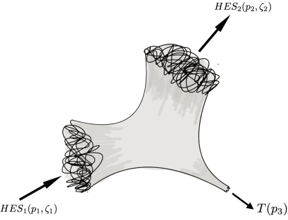
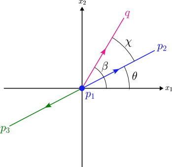
Figure 1: Left Panel : The 3 point scattering set-up considered. Right Panel : Kinematics with angles indicated, green arrows indicate tachyons, while blue the $HES$ ones. $HES_{1}$ is initially at rest, the pink arrow indicates the photon momenta which make up the $|HES\rangle$ states.

The final amplitude is obtained after two steps. Firstly we need to carry out contractions of the relevant string vertex operators, next we need to integrate over the vertex coordinates. The integrand that we need to compute is given by:

$$e^{\cal L} =\langle:\prod_{r_{1}}\left(\sum_{m_{1}}^{r_{1}}{i\over(m_{1}-1)!}\zeta_{1}\cdot\partial^{m_{1}}X_{1}S^{1}_{r_{1}-m_{1}}\right)e^{ip_{1}\cdot X_{1}}::\prod_{r_{2}}\left(\sum_{m_{2}}^{r_{2}}{i\over(m_{2}-1)!}\zeta_{2}\cdot\partial^{m_{2}}X_{2}S^{2}_{r_{2}-m_{2}}\right)e^{ip_{2}\cdot X_{2}}:$$

$$:e^{ip_{3}\cdot X_{3}}:\rangle$$ (2.3)

We evaluate the contractions using the identities:

$$\langle X^{\mu}(z)X^{\nu}(w)\rangle =-\eta^{\mu\nu}\log(z-w),\qquad\langle\partial_{z}X^{\mu}(z)X^{\nu}(w)\rangle=-\eta^{\mu\nu}{1\over(z-w)},$$ (2.4)

$$\langle\partial_{z}X^{\mu}(z):e^{ik.X(w)}:\rangle =-{ik^{\mu}\over(z-w)}:e^{ik.X(w)}:,\qquad\langle:e^{ik_{1}.X(z)}::e^{ik_{2}.X(w)}:\rangle=(z-w)^{k_{1}.k_{2}}.$$

Carrying out all possible contractions on the right hand side of Eq.(2.3) yields:

$$\begin{split}\sum_{k=0}^{\{J_{1},J_{2}\}_{min}}\sum_{\begin{subarray}{c}\{a(k)\}\subset\{r_{1}\}\\ \{b{(k)}\}\subset\{r_{2}\}\\ \text{ordered}\end{subarray}}{1\over k!}&\prod_{i=1}^{k}\Bigg{[}\sum_{m_{1},m_{2}=1}^{a_{i},b_{i}}\bigg{\{}{(-1)^{m_{2}+1}(m_{1}+m_{2}-1)!\zeta_{1}.\zeta_{2}\over(m_{1}-1)!(m_{2}-1)!z_{21}^{m_{1}+m_{2}}}\bigg{\}}\\ &\;\ \;\ \;\ \;\ \;\ \;\ \times S_{a_{i}-m_{1}}\bigg{(}{a_{i}\over s_{1}}\left({q_{1}\cdot p_{2}\over z_{21}^{s_{1}}}+{q_{1}\cdot p_{3}\over z_{31}^{s_{1}}}\right)\bigg{)}S_{b_{i}-m_{2}}\bigg{(}{b_{i}\over s_{2}}\left({q_{2}\cdot p_{1}\over z_{12}^{s_{2}}}+{q_{2}\cdot p_{3}\over z_{32}^{s_{2}}}\right)\bigg{)}\Bigg{]}\\ \times&\prod_{l_{1}\in\overline{\{a(k)\}}}\Bigg{[}\sum_{n_{1}=1}^{l_{1}}\bigg{(}{\zeta_{1}\cdot p_{2}\over z_{21}^{n_{1}}}+{\zeta_{1}\cdot p_{3}\over z_{31}^{n_{1}}}\bigg{)}S_{l_{1}-n_{1}}\Bigg{]}\\ \times&\prod_{l_{2}\in\overline{\{b(k)\}}}\Bigg{[}\sum_{n_{2}=1}^{l_{2}}\bigg{(}{\zeta_{2}\cdot p_{1}\over z_{12}^{n_{2}}}+{\zeta_{2}\cdot p_{3}\over z_{32}^{n_{2}}}\bigg{)}S_{l_{2}-n_{2}}\Bigg{]}\times\prod_{i<j}z_{ij}^{p_{i}\cdot p_{j}}=B_{\{r_{1}\},\{r_{2}\}}\prod_{i<j}z_{ij}^{p_{i}\cdot p_{j}}.\end{split}$$ (2.5)

The first term in the square bracket includes terms coming from contractions among the DDF vertex operators. The sum over $\{a(k)\}$ and, $\{b(k)\}$ denote the different ordered subsets of partitions of $N_{1}$ and $N_{2}$, which are $\{r_{1}\}$ and, $\{r_{2}\}$ respectively. They have $k$ elements each, which get contracted. Taking ordered subset is important because we want to include all possible $k$-term contractions for different values of $k$. For example if $k=2$ then $\{a(k)\}_{1}=\{a_{1},a_{2}\}\;\ ;\;\ \{a(k)\}_{2}=\{a_{2},a_{1}\}\;\ ;\;\ \{b(k)\}_{1}=\{b_{1},b_{2}\}\;\ ;\;\ \{b(k)\}_{2}=\{b_{2},b_{1}\}$ must be considered in order to consider all possible contractions i.e. $p(a_{1},b_{1})\times p(a_{2},b_{2})$ and $p(a_{1},b_{2})\times p(a_{2},b_{1})$. We have to divide by ${k!}$ to compensate for the overcounting.

The number of such contractions depend on the number of $A_{-r}$’s present in a DDF factor. This is given by $J=\sum_{r}n_{r}$, where $n_{r}$ counts the repeatitions of the mode $r$ in the partition $\{r\}$. Since there are two DDF factors the maximum contractions $k$, is given by the minimum among $J_{1}$ and $J_{2}$. The complementary subsets are the remaining operators that get contracted amongst each other to produce the products of the second and the third square brackets of Eq.(4.3).

Finally, in writing down the result we also make the choice of $q_{1}\propto q_{2}$. This gets rid of contractions between the derivatives and the arguments of the Schur polynomials. The integrand can finally be expressed as:

$${\cal L} =\sum_{i<j}p_{i}\cdot p_{j}\log z_{ij}+\log B_{\{r_{1}\},\{r_{2}\}}.$$ (2.6)

If we reinstate the $\alpha^{\prime}$ dependence we obtain:

$$\sum_{k=0}^{\{J_{1},J_{2}\}_{min}}\sum_{\begin{subarray}{c}\{a(k)\}\subset\{r_{1}\}\\ \{b{(k)}\}\subset\{r_{2}\}\\ \text{ordered}\end{subarray}}{1\over k!}\prod_{i=1}^{k}\Bigg{[}\sum_{m_{1},m_{2}=1}^{a_{i},b_{i}}\bigg{\{}{(-1)^{m_{2}+1}(m_{1}+m_{2}-1)!\zeta_{1}.\zeta_{2}\over(m_{1}-1)!(m_{2}-1)!z_{21}^{m_{1}+m_{2}}}\bigg{\}}S_{a_{i}-m_{1}}\bigg{(}{2\alpha^{\prime}a_{i}\over s_{1}}\left({q_{1}\cdot p_{2}\over z_{21}^{s_{1}}}+{q_{1}\cdot p_{3}\over z_{31}^{s_{1}}}\right)\bigg{)}$$

$$S_{b_{i}-m_{2}}\bigg{(}{2\alpha^{\prime}b_{i}\over s_{2}}\left({q_{2}\cdot p_{1}\over z_{12}^{s_{2}}}+{q_{2}\cdot p_{3}\over z_{32}^{s_{2}}}\right)\bigg{)}\Bigg{]}\prod_{l_{1}\in\overline{\{a(k)\}}_{i}}\Bigg{[}\sum_{n_{1}=1}^{l_{1}}\sqrt{2\alpha^{\prime}}\bigg{(}{\zeta_{1}\cdot p_{2}\over z_{21}^{n_{1}}}+{\zeta_{1}\cdot p_{3}\over z_{31}^{n_{1}}}\bigg{)}S_{l_{1}-n_{1}}\Bigg{]}$$ (2.7)

$$\times\prod_{l_{2}\in\overline{\{b(k)\}}_{j}}\Bigg{[}\sum_{n_{2}=1}^{l_{2}}\sqrt{2\alpha^{\prime}}\bigg{(}{\zeta_{2}\cdot p_{1}\over z_{12}^{n_{2}}}+{\zeta_{2}\cdot p_{3}\over z_{32}^{n_{2}}}\bigg{)}S_{l_{2}-n_{2}}\Bigg{]}\times\prod_{i<j}z_{ij}^{2\alpha^{\prime}p_{i}\cdot p_{j}}.$$

After plugging in the kinematic choices during the explicit evaluation of the amplitude, the $\alpha^{\prime}$ factors all drop out.

2.1 Kinematics for $HHT$

We follow the metric signature $(-,+,+\dots+)$. Therefore the on-shell condition is $p_{i}^{2}=-M_{i}^{2}$. Furthermore we take all the momenta to be ingoing. We choose the frame such that $|HES_{1}\rangle$ with rest mass $\sqrt{2(N_{1}-1)}$ decays into a tachyon of rest mass squared $-2$ and $|HES_{2}\rangle$ with rest mass $\sqrt{2(N_{2}-1)}$. We parametrize the ground state momenta as:

String States Final Momenta

The list of constraints are,

$$\left(p_{1}\right)^{2}=-M_{1}^{2}=-2(N_{1}-1),\quad\left(p_{2}\right)^{2}=-M_{2}^{2}=-2(N_{2}-1),$$

$$\left(p_{3}\right)^{2}=2,\quad p_{1}+p_{2}+p_{3}=0.$$ (2.8)

Maintaining the constraints we choose:

$$p_{1} =\sqrt{2(N_{1}-1)}(1,0,0),\,\,\,p_{2}=-\sqrt{2(N_{2}-1)}\left({N_{1}+N_{2}-1\over\sqrt{2(N_{1}-1)}\sqrt{2(N_{2}-1)}},\kappa\cos\theta,\kappa\sin\theta\right)\quad$$

$$p_{3} =-\left({N_{1}-N_{2}-1\over\sqrt{2(N_{1}-1)}},-\kappa\sqrt{2(N_{2}-1)}\cos\theta,-\kappa\sqrt{2(N_{2}-1)}\sin\theta\right),$$ (2.9)

$$\text{where}\;\kappa=\sqrt{{(N_{1}+N_{2}-1)^{2}\over 2(N_{1}-1)2(N_{2}-1)}-1}.$$

DDF Photon Momenta

We take these photons of both the $|HES\rangle$ to be parallel i.e. $q_{1}\propto q_{2}$, i.e, $q_{1}\equiv q,~{}q_{2}\equiv-\gamma q$. Temporal component of DDF photon associated with $|HES_{2}\rangle$ is negative, which is fixed by the sign of $\gamma$, see Appendix §A. Furthermore we also need $q_{1}^{2}=0$ and $q\cdot\tilde{p}_{1}=0$. These are satisfied by:

$$\begin{split}&q=-{1\over\sqrt{2(N_{1}-1)}}\left(1,\cos(\beta),\sin(\beta)\right)\\ \text{where, }&\beta=\theta+\sec^{-1}\left({-\gamma\sqrt{(N_{1}-N_{2})^{2}+2(N_{1}+N_{2})-3}\over(2-\gamma)N_{1}-\gamma(N_{2}-1)-2}\right)\end{split}$$ (2.10)

We can argue that $\gamma$ is strictly positive so that we maintain $q_{2}\cdot\tilde{p}_{2}=-\gamma q_{1}\cdot\tilde{p}_{2}=1$ (See Appendix §A). Next, recall for DDF states : $\zeta=\lambda-(p\cdot\lambda)q$. In what follows we work with two choices of polarization inner products.

• $\mathbf{\lambda_{1}\cdot\lambda_{2}=0}$ : For the photon polarization, we take $\lambda_{2}=-\lambda_{1}=-\lambda$, which satisfies $q.\lambda=0,~{}\lambda^{2}=0$. Then $\lambda$ can be written in terms of $\beta$ as :

  $$\lambda={1\over\sqrt{2}}\left(0,\sin(\beta),-\cos(\beta),i\right).$$

  Note that for this choice of polarization $\zeta_{1}\cdot\zeta_{2}=0$ and thus this choice hides the effect of the derivative contractions among the $|HES\rangle$ states.

• $\mathbf{\lambda_{1}\cdot\lambda_{2}\neq 0}$ : The other choice of polarizations maintaining $\lambda_{1}^{2}=\lambda_{2}^{2}=\lambda_{1}\cdot q_{1}=\lambda_{2}\cdot q_{2}=0$ is :

  $$\lambda_{1} ={1\over\sqrt{2}}\left(0,\sin(\beta),-\cos(\beta),i\right),\quad\lambda_{2}={1\over\sqrt{2}}\left(0,\sin(\beta),-\cos(\beta),-i\right).$$ (2.11)

  Note that automatically $\lambda_{1}\cdot q_{2}=\lambda_{2}\cdot q_{1}=0$ is also guaranteed. And now, the dot product gives:

  $$\zeta_{1}\cdot\zeta_{2} =\lambda_{1}\cdot\lambda_{2}=1.$$ (2.12)

We will consider and contrast the amplitudes for both of these choices.

2.2 Evaluating the $HHT$ amplitude

The tachyon contraction factor of Eq.(2.6) can be explicitly evaluated using the constraint relations in (2.8). We replace $p_{3}$ in our computation as it turns out that the final relations are relatively simpler compared to any other substitutions,

$$\underset{i<j}{\sum}p_{i}.p_{j}\log z_{ij} =p_{1}.p_{2}\log z_{12}+p_{1}.p_{3}\log z_{13}+p_{2}.p_{3}\log z_{23}$$

$$=p_{1}.p_{2}\log z_{12}-p_{1}.(p_{1}+p_{2})\log z_{13}-p_{2}.(p_{1}+p_{2})\log z_{23}$$

$$=\log\left({z_{12}^{N_{1}+N_{2}}\over z_{13}^{N_{2}-N_{1}}z_{23}^{N_{1}-N_{2}}}\right)+\log\left({1\over z_{12}z_{13}z_{23}}\right).$$

Therefore we write Eq.(2.6) as:

$$\int\prod_{i}dz_{i}\;\ e^{\mathcal{L}}=\int{dz_{1}dz_{2}dz_{3}\over z_{12}z_{13}z_{23}}\exp\left(\log\left({z_{12}^{N_{1}+N_{2}}\over z_{13}^{N_{2}-N_{1}}z_{23}^{N_{1}-N_{2}}}\right)+\log B_{\{r_{1}\},\{r_{2}\}}\right).$$ (2.13)

The quantity in front of the exponential with the measure becomes $SL_{2}$ invariant. Thus by using $SL_{2}$ invariance and fixing, $z_{1}=0,z_{2}=1$ and $z_{3}=\infty$ (which is decided by the first term in the exponent), we can get rid of the integrals completely. Finally, the total amplitude becomes:

$$\begin{split}\mathcal{A}=\sum_{k=0}^{min\{J_{1},J_{2}\}}{1\over k!}\sum_{\begin{subarray}{c}\{a(k)\}\\ \{b(k)\}\\ \text{ordered}\end{subarray}}\left(\prod_{i=1}^{k}P(a_{i},b_{i})\prod_{l_{1}\in\overline{\{a(k)\}}}Q_{1}(l_{1})\prod_{l_{2}\in\overline{\{b(k)\}}}Q_{2}(l_{2})\right),\end{split}$$ (2.14)

where, $P(a_{i},b_{i}),~{}Q_{1}(l_{1})~{}\text{and}~{}Q_{2}(l_{2})$ are given as below,

$$P(a_{i},b_{i}) =\sum_{m_{1},m_{2}=1}^{a_{i},b_{i}}(-1)^{m_{2}+1}\bigg{[}(\zeta_{1}\cdot\zeta_{2}){(m_{2}+m_{1}-1)!\over(m_{1}-1)!(m_{2}-1)!}S_{a_{i}-m_{1}}\bigg{(}-{a_{i}\over s_{1}\gamma}\bigg{)}S_{b_{i}-m_{2}}\bigg{(}-{b_{i}(-1)^{s_{2}}\over s_{2}}\gamma\bigg{)}\bigg{]}$$ (2.15)

$$Q_{1}(l_{1}) =\sum_{m_{1}=1}^{l_{1}}(\zeta_{1}\cdot p_{2})S_{l_{1}-m_{1}}\bigg{(}-{l_{1}\over s_{1}\gamma}\bigg{)}=(\zeta_{1}\cdot p_{2})V_{1}(l_{1})$$ (2.16)

$$Q_{2}(l_{2}) =\sum_{m_{2}=1}^{l_{2}}(\zeta_{2}\cdot p_{1})(-1)^{m_{2}}S_{l_{2}-m_{2}}\bigg{(}-{l_{2}(-1)^{s_{2}}\over s_{2}}\gamma\bigg{)}=(\zeta_{2}\cdot p_{1})V_{2}(l_{2})$$ (2.17)

Note that the arguments in the Schur polynomials have simplified, in fact they can now be expressed in terms of products :

$$S_{r_{1}-m_{1}} ={(-1)^{r_{1}-m_{1}}\over(r_{1}-m_{1})!}\prod_{s_{1}=1}^{r_{1}-m_{1}}\bigg{(}{r_{1}\over\gamma}-s_{1}+1\bigg{)},\,\,S_{r_{2}-m_{2}}={1\over(r_{2}-m_{2})!}\prod_{s_{2}=1}^{r_{2}-m_{2}}\bigg{(}r_{2}\gamma-s_{2}+1\bigg{)}.$$ (2.18)

Next, we can simplify Eq.(2.15) as:

$$P(a_{i},b_{i}) =\sum_{m_{1},m_{2}=1}^{a_{i},b_{i}}{(-1)^{m_{2}+1+a_{i}-m_{1}}\over(a_{i}-m_{1})!(b_{i}-m_{2})!}\bigg{[}{(m_{2}+m_{1}-1)!\over(m_{1}-1)!(m_{2}-1)!}\bigg{]}\prod_{s_{1}=1}^{a_{i}-m_{1}}\bigg{(}{a_{i}\over\gamma}-s_{1}+1\bigg{)}$$

$$\times\prod_{s_{2}=1}^{b_{i}-m_{2}}\bigg{(}b_{i}\gamma-s_{2}+1\bigg{)}$$

$$=(-1)^{a_{i}}\prod_{j_{1}=1}^{a_{i}-1}\left({a_{i}/\gamma-a_{i}+j_{1}\over j_{1}}\right)\prod_{j_{2}=1}^{b_{i}-1}\bigg{(}{b_{i}\gamma-b_{i}+j_{2}\over j_{2}}\bigg{)}\bigg{(}{(\gamma-1)a_{i}b_{i}\over a_{i}-b_{i}\gamma}\bigg{)}$$

$$=(-1)^{a_{i}}\prod_{j_{1}=1}^{a_{i}-1}\left({a_{i}/\gamma-j_{1}\over j_{1}}\right)\prod_{j_{2}=1}^{b_{i}-1}\bigg{(}{b_{i}\gamma-j_{2}\over j_{2}}\bigg{)}\bigg{(}{(\gamma-1)a_{i}b_{i}\over a_{i}-b_{i}\gamma}\bigg{)}.$$ (2.19)

Similarly, carrying out the sums in equation (2.16) and equation (2.17) yields simpler product formula expressions of $Q_{1}$ and $Q_{2}$,

$$Q_{1}(l_{1}) =(\zeta_{1}\cdot p_{2})(-1)^{l_{1}}\prod_{j_{1}=1}^{l_{1}}\left({l_{1}/\gamma-j_{1}\over j_{1}}\right)$$ (2.20)

$$=-\left(\sqrt{{N_{1}+N_{2}-1\over\gamma}-{N_{1}-1\over\gamma^{2}}-(N_{2}-1)}\right)(-1)^{l_{1}}\prod_{j_{1}=1}^{l_{1}}\left({l_{1}/\gamma-j_{1}\over j_{1}}\right)$$ (2.21)

$$Q_{2}(l_{2}) =(\zeta_{2}\cdot p_{1})\prod_{j_{2}=1}^{l_{2}}\left({l_{2}\gamma-j_{2}\over j_{2}}\right)$$ (2.22)

$$=-\left(\sqrt{(N_{1}+N_{2}-1)\gamma-(N_{1}-1)-(N_{2}-1)\gamma^{2}}\right)\prod_{j_{2}=1}^{l_{2}}\left({l_{2}\gamma-j_{2}\over j_{2}}\right).$$

We can express the amplitude also in terms of $\chi=\beta-\theta,\bar{N}=N_{1}+N_{2}$ and $\bar{n}=N_{1}-N_{2}$ by substituting:

$$\gamma ={2(N_{1}-1)\over\bar{N}-1-(\cos\chi)\sqrt{2\bar{N}+\bar{n}^{2}-3}}.$$ (2.23)

3 Averaging the $HHT$ scattering amplitude

In this section we average over $HES$ states belonging to the same level (mass). This translates to averaging over different partitions. This averaging takes the form:

$$\langle{\mathcal{A}_{(\{r_{1}\},\{r_{2}\})}}\rangle_{F}\sim(-1)^{N}\equiv{1\over\Omega(N_{1})\Omega(N_{2})}\sum_{\{n_{1}\},\{n_{2}\}}\mathcal{A}\left(\{n_{1}\},\{n_{2}\}\right),$$ (3.1)

where $\Omega(N)$ counts the number of $|HES\rangle$ microstates at the fixed level $N$. At large $N$ for fixed polarization a large $N$ calculation shows: $\Omega(N)\sim\exp\left(2\pi\sqrt{N}/\sqrt{6}\right)$. We are able to analytically carry out averaging in the kinematic choice where $\zeta_{1}\cdot\zeta_{2}=0$. Now the amplitude is of the product form

$$\mathcal{A}_{(\{r_{1}\},\{r_{2}\},\zeta_{1}\cdot\zeta_{2}=0)}=\prod_{r_{1}}\left(\zeta_{1}\cdot p_{2}V_{1}(r_{1})\right)^{n_{r_{1}}}\prod_{r_{2}}\left(\zeta_{2}\cdot p_{1}V_{2}(r_{2})\right)^{n_{r_{2}}},$$

where the exact form of the $V_{1}$ and $V_{2}$ (as defined in Eq.(2.17)) are:

$$V_{1}(r_{1}) =(-1)^{r_{1}}\prod_{j_{1}=1}^{r_{1}-1}\bigg{(}{r_{1}/\gamma-j_{1}\over j_{1}}\bigg{)},\quad V_{2}(r_{2})=\prod_{j_{2}=1}^{r_{2}-1}\bigg{(}{r_{2}\gamma-j_{2}\over j_{2}}\bigg{)}.$$ (3.2)

Therefore the full averaged amplitude becomes :

$$\langle{{\cal A}}\rangle_{F} =\sum_{\begin{subarray}{c}\{n_{r_{1}}\}\\ \{n_{r_{2}}\}\end{subarray}}{1\over\Omega(N_{1})\Omega(N_{2})}\oint d\beta_{1}d\beta_{2}\,\,e^{\beta_{1}N_{1}+\beta_{2}N_{2}}e^{-\beta_{1}\sum_{r_{1}}r_{1}n_{r_{1}}}e^{-\beta_{2}\sum_{r_{2}}r_{2}n_{r_{2}}}\mathcal{A}_{(\{r_{1}\},\{r_{2}\},\zeta_{1}\cdot\zeta_{2}=0)}$$

$$=\sum_{\begin{subarray}{c}n_{r_{1}}=0\\ n_{r_{2}}=0\end{subarray}}^{\infty}{1\over\Omega(N_{1})\Omega(N_{2})}\oint d\beta_{1}d\beta_{2}\,\,e^{\beta_{i}N_{i}}\prod_{r_{1}=1}^{\infty}e^{-\beta_{1}r_{1}n_{r_{1}}}q_{1}(r_{1})\prod_{r_{2}=1}^{\infty}e^{-\beta_{2}r_{2}n_{r_{2}}}q_{2}(r_{2})$$ (3.3)

$$={1\over\Omega(N_{1})\Omega(N_{2})}\oint d\beta_{1}d\beta_{2}\,\,e^{\beta_{i}N_{i}}\prod\limits_{r_{1}\in\{N_{1}\}}\bigg{(}1-e^{-\beta_{1}r_{1}}(\zeta_{1}\cdot p_{2})V_{1}\bigg{)}^{-1}\prod\limits_{r_{2}\in\{N_{2}\}}\bigg{(}1-e^{-\beta_{2}r_{2}}(\zeta_{2}\cdot p_{1})V_{2}\bigg{)}^{-1}.$$

We evaluate the above expression for $N_{1}=N_{2}=N$ and $N\rightarrow\infty$. The variable $\gamma$ takes the form

$$\begin{split}\gamma&=1+\sqrt{{1\over{N}}}\cos(\chi)+{\cos(2\chi)\over{N}}+O\left(\left({1\over{2N}}\right)^{3/2}\right)\simeq 1+\delta,\end{split}$$ (3.4)

with $\delta\ll 1$. Using this expansion of $\gamma$ in large $N$ limit, the expansions of the other factors, till leading order follows:

$$V_{1}(r_{1}) \sim(-1)^{r_{1}}+\mathcal{O}(\delta),\,\,\,V_{2}(r_{2})\sim 1+\mathcal{O}(\delta),\,\,\,(\zeta_{1}\cdot p_{2}) \sim-\sin\chi,\,\,\,(\zeta_{2}\cdot p_{1})\sim-\sin\chi.$$ (3.5)

Plugging these into Eq.(3.1) we obtain:

$$\langle\mathcal{A}\rangle_{F} \simeq{(-1)^{N}\over\Omega_{1}(N)\Omega_{2}(N)}\oint d\beta_{1}e^{\beta_{1}N}\prod_{r_{1}}\left(1+\sin\chi(e^{-\beta_{1}})^{r_{1}}\right)^{-1}\oint d\beta_{2}e^{\beta_{2}N}\prod_{r_{2}}\left(1+\sin\chi(e^{-\beta_{2}})^{r_{2}}\right)^{-1}.$$ (3.6)

At large $N$ we expect the saddle point of $\beta_{i}$ integrals to be dominated by small values. It is under this expectation that the products maybe evaluated in terms of dilogarithm function:

$$\prod_{r_{1}}\left(1+\sin\chi(e^{-\beta_{1}})^{r_{1}}\right)^{-1} =\exp\left[-\sum_{r_{1}=1}^{\infty}\log\big{(}1+\sin\chi(e^{-\beta_{1}})^{r_{1}}\big{)}\right]=\exp\left[\sum_{k=1}^{\infty}{(-\sin\chi)^{k}\over k\big{(}e^{\beta_{1}k}-1\big{)}}\right]$$

$$\simeq\exp\left[\sum_{k=1}^{\infty}{(-\sin\chi)^{k}\over k^{2}\beta_{1}}\right]=\exp\left[{1\over\beta_{1}}\text{Li}_{2}(-\sin\chi)\right].$$ (3.7)

The saddle of the $\beta_{1}$ and $\beta_{2}$ integrals are at, $\beta_{i}^{*}=\sqrt{{1\over N}\text{Li}_{2}(-\sin\chi)}.$ Hence each of the on-shell integrals evaluates to:

$$\oint d\beta_{2}e^{\beta_{2}N}\prod_{r_{2}}\left(1+\sin\chi(-e^{-\beta_{2}})^{r_{2}}\right)^{-1} \simeq\exp\left[2\sqrt{N}\sqrt{\text{Li}_{2}(-\sin\chi)}\right].$$ (3.8)

Collecting all the factors we obtain:

$$\langle\mathcal{A}\rangle_{F} \simeq(-1)^{N}\exp\Bigg{[}4\sqrt{N}\bigg{(}\sqrt{\text{Li}_{2}(-\sin\chi)}-{\pi\over\sqrt{6}}\bigg{)}\Bigg{]}.$$ (3.9)

The diagonal piece at same level

Out of the summation we can separate out the diagonal piece, i.e., the contribution coming from terms where both the in and the out states are described by identical partitions. This is given by:

$$\langle{{\cal A}}\rangle_{D} =\sum_{\{n_{r}\}}{1\over\Omega(N)}\oint d\beta\,\,e^{\beta N}e^{-\beta\sum_{r}rn_{r}}\mathcal{A}_{(\{n_{r}\},\{n_{r}\},\zeta_{1}\cdot\zeta_{2}=0)}$$

$$=(-1)^{N}\sum_{\{n_{r}\}}^{\infty}{1\over\Omega(N)}\oint d\beta\,\,e^{\beta N}\prod_{r=1}^{\infty}e^{-\beta rn_{r}}\left(\sin^{2}\chi\right)^{n_{r}}$$ (3.10)

$$=(-1)^{N}{1\over\Omega(N)}\oint d\beta\,\,e^{\beta N}\prod\limits_{r=1}^{\infty}{1\over 1-\sin^{2}\chi e^{-\beta r}}.$$

Once again anticipating a small $\beta$ saddle we carry out the manipulations as in Eq.(3.7) which gives :

$$\prod_{r}{1\over\left(1-\sin^{2}\chi(e^{-\beta r})\right)}=\exp\left[{1\over\beta}\text{Li}_{2}(\sin^{2}\chi)\right].$$ (3.11)

Therefore the saddle point is now at: $\beta^{*}=\sqrt{{1\over N}\text{Li}_{2}(\sin^{2}\chi)}$ which implies:

$$\langle{{\cal A}}\rangle_{D}=(-1)^{N}\exp\left[2\sqrt{N}\bigg{\{}\sqrt{\text{Li}_{2}(\sin^{2}\chi)}-{\pi\over\sqrt{6}}\bigg{\}}\right].$$ (3.12)

Comparison with the thermal one-point function

To compare with the thermal one point function we need to consider only the diagonal matrix elements, i.e., $|HES\rangle$ states having identical partitions. Therefore the relevant expression is the coarse-grained expression as given above in Eq.(3.12). It turns out that the function $\sqrt{\text{Li}_{2}(\sin^{2}\chi)}$ has a maxima at $\chi=\pi/2$. Very interestingly, the value at this maximum $\text{Li}_{2}(1)={\pi^{2}\over 6}$ exactly cancels with the entropic normalization factor in the exponent. Hence if we sum over all the angles, then upto exponentially small corrections :

$$\langle{A}\rangle_{D}\sim 1+{\cal{O}}\left(e^{-\sqrt{N}}\right),$$ (3.13)

where the ${\cal{O}}(1)$ leading term comes from $\chi=\pi/2$. In analogy with ETH, Eq. (1.3), we will like to identify this diagonal piece with the thermal one point function. And, since this is the one-point function computed in the coarse-grained $|HES\rangle$ background, we will compare this with the black hole one point function, where the black hole is at the correspondence point. In the $AdS/CFT$ context, [36] pointed out that the CFT thermal one point function, under suitable analytic continuation of the conformal dimension of the operator, contains a phase which probes the geometry behind the horizon: $\langle{O}\rangle_{\beta}\sim\exp\left(-i\,m\,t_{s}\right)$, where $t_{s}$ is the time to singularity in an asymptotically $AdS$ black hole. This identification has been shown to hold rigorously for many generalizations [50]. The correspondence point black hole is described by the Schwarzchild metric, which in $d=4$ is :

$$ds^{2} =-\left(1-{2GM\over r}\right)dt^{2}+\left(1-{2GM\over r}\right)^{-1}dr^{2}+r^{2}d\Omega^{2}.$$ (3.14)

It turns out that the time to the singularity for the above metric yields a finite quantity :

$$t_{s} =\lim_{\epsilon\rightarrow 0}\int_{2GM}^{\epsilon}{dr\over-\sqrt{{2GM\over r}-1}}=G\,M\pi+{\cal{O}}\left(\epsilon^{3/2}\right).$$ (3.15)

Note, unlike $AdS$ the $t_{s}$ depends explicitly on the black hole mass, also note that we work with the negative square-root to get a positive physical infall time. Hence we expect that:

$$\langle{O}\rangle_{\beta} =\exp\bigg{[}{\pi\,G\,M\over\sqrt{\alpha^{\prime}}}\bigg{]}=\exp\bigg{[}\pi\sqrt{\alpha^{\prime}}g_{s}^{2}\,M\bigg{]}.$$ (3.16)

In the above we used the tachyon mass $=i/\sqrt{\alpha^{\prime}}$ and the gravitational coupling $G=g_{s}^{2}\alpha^{\prime}$. Now at the correspondence point $g_{s}^{2}M=1/\sqrt{\alpha^{\prime}}$, hence we are simply left with an ${\cal{O}}(1)$ real number $\sim e^{\pi}$. In this sense it is consistent with the ${\cal{O}}(1)$ number obtained in Eq. (3.13).

The off-diagonal piece at same level

We can now write the off-diagonal averaged amplitude in terms of Eq.(3.1) and Eq.(3.12) :

$$\langle{\mathcal{A}}\rangle_{OD} \sim{1\over\Omega(N)^{2}-\Omega(N)}\sum_{\begin{subarray}{c}\{n_{1}\},\{n_{2}\}\\ {n_{1}}\neq{n_{2}}\end{subarray}}\mathcal{A}\left(\{n_{1}\},\{n_{2}\}\right)\simeq{1\over\Omega(N)^{2}}\left(\sum_{\{n_{1}\},\{n_{2}\}}\mathcal{A}\left(\{n_{1}\},\{n_{2}\}\right)-\sum_{\{n\}}\mathcal{A}\left(\{n\},\{n\}\right)\right)$$

$$={1\over\Omega(N)^{2}}\left(\Omega(N)^{2}\langle{\mathcal{A}}\rangle_{F}-\Omega(N)\langle{\mathcal{A}}\rangle_{D}\right)$$ (3.17)

$$=(-1)^{N}\left(\exp\left[4\sqrt{N}\left\{\sqrt{\text{Li}_{2}(-\sin\chi)}-{\pi\over\sqrt{6}}\right\}\right]-\exp\left[2\sqrt{N}\left\{\sqrt{\text{Li}_{2}(\sin^{2}\chi)}-{2\pi\over\sqrt{6}}\right\}\right]\right)$$

$$\equiv(-1)^{N}\left(ue^{i\phi}-v\right).$$

where we have defined real quantities $u,v$ and $\phi$ through:

$$u\equiv \exp\left({-4\pi\over\sqrt{6}}\sqrt{N}\right),~{}v\equiv\exp\left[2\sqrt{N}\left\{\sqrt{\text{Li}_{2}(\sin^{2}\chi)}-{2\pi\over\sqrt{6}}\right\}\right]$$ (3.18)

$$e^{i\phi} \equiv\exp\left[4\sqrt{N}\sqrt{\text{Li}_{2}(-\sin\chi)}\right]~{}\text{as }\text{Li}_{2}(-\sin\chi)\leq 0\text{ for }0\leq\chi\leq\pi.$$

Therefore the absolute value squared which is $|\langle{\mathcal{A}}\rangle_{OD}|^{2}=u^{2}+v^{2}-2uv\cos\phi$ is bounded by:

$$(u-v)^{2}\leq|\langle{\mathcal{A}}\rangle_{OD}|^{2}\leq(u+v)^{2}.$$

At large $N$ the upper bound behaves as, $\sim\exp\left[-2\sqrt{N}\left({2\pi\over\sqrt{6}}-\sqrt{\text{Li}_{2}(\sin^{2}\chi)}\right)\right]$. Since ${\text{Li}_{2}(1)}=\pi/\sqrt{6}$, which is its maximum value, we obtain:

$$|\langle{\mathcal{A}}\rangle_{OD}|\leq\exp\left(-{2\pi\over\sqrt{6}}\sqrt{N}\right)\sim\left(\Omega(N)\right)^{-1}.$$ (3.19)

Hence, when the microstates are not the same, there is entropic suppression. In §3.1 we will numerically probe off-diagonal elements at different levels which apart from coming with the entropic suppression, also turns out to contain the decaying factor $f_{O}(\omega)$ consistent with ETH, Eq.(1.3).

3.1 Numerically probing chaos and the ETH

As for the general formula for the amplitude in Eq.(2.14) it is difficult to implement the coarse-graining analytically, here we investigate its features numerically.

3.1.1 Signatures of RMT chaos in the $HHT$ amplitude

As indicated in [26, 30] we focus on the resonance peak statistics to probe chaos. We consider the $HHT$ amplitude for all the partitions of $N_{1}=N_{2}=N$. The steps of the numerics are following:

1. For two fixed partitions $N$ : $\{r_{1}\},\{r_{2}\}$ amplitude $\mathcal{A}(\chi)$ is evaluated in the range of $\chi=\left[0,\pi\right]$ with step size of $\delta\chi=0.001$.

2. From the amplitude array, the peak positions of $\mathcal{A}(\chi)$ are found out by checking which $\{\chi_{*}\}_{\{r_{1}\},\{r_{2}\}}$ values satisfy $\mathcal{A}^{\prime}(\chi_{*})=0$.

3. We repeat the above two steps for all possible sets $\{r_{1}\},\{r_{2}\}$ and keep adding to : $\{\chi_{*}\}$. Next, the probability distribution of these peak positions and the spacings between the adjacent peaks are studied.

Choosing different values of $N$, the numerical analysis has been done both for the $\zeta_{1}\cdot\zeta_{2}=1$ as well as the orthogonal polarization case. To look into the chaotic features of the amplitude, we look at the level statistics and find numerical evidence of level repulsion. See left panel of Fig.2 where we present the histograms for the $\zeta_{1}\cdot\zeta_{2}=0$ cases. This feature was also noted for the $HTT$ amplitude in [30], hence is not surprizing that it continues to hold for the $HHT$ case. However the availability of more states allows for better coarse-grainings, for instance for the $N=20$ case we have peak statistics from $393129$ matrix elements as function of $\chi$.

We will like to contrast this distribution with that obtained from random matrix theory. In particular we compare the $HHT$ peak level statistics distribution with the level statistics of Gaussian orthogonal ensemble of RMT. Our measure is the Kolmogorov-Smirnov (KS) test. This compares the empirical cumulative distribution (ECDF) functions of two data sets and provides a measure to decide how close the two distributions are. The ECDF of a given data set $\{x_{1},\cdots,x_{n}\}$ is: $F_{n}(x)=\tfrac{\text{number of elements $\{x_{i}\}\leq x$}}{n}$ The KS statistic for a given CDF $F(x)$ is defined via: $D_{n}=\sup_{x}|F_{n}(x)-F(x)|$. Thus smaller $D_{n}$ indicates that he two distributions are closer. Here, we take $F(x)$ from GOE Wigner-Dyson distribution and compare it with the ECDF derived from the peak statistics. In the right panel of Fig.2 we show that as $N$ increases the level spacing distribution indeed gets closer to that which follows from the GOE.

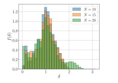
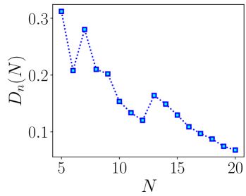
Figure 2: Left Panel : Plot of the peak level spacing statistics of the amplitude with $\zeta_{1}\cdot\zeta_{2}=0$. Right Panel : KS statistical distance between the level spacing statistics cumulative distribution of the amplitude and GOE random matrix statistics.

Next we perform the KS test for same values of $N$ for the two cases of $\zeta_{1}\cdot\zeta_{2}$, see Fig.3. It is found that a non-zero inner product between the polarizations approach the chaotic distribution for a smaller $N$ compared to the orthogonally polarized case. A likely explanation for this difference is the fact that $\zeta_{1}\cdot\zeta_{2}=0$ is a more restrictive kinematic choice than $\zeta_{1}\cdot\zeta_{2}\neq 0$. In particular, for the latter the phase space volume being more, notions of ETH are satisfied at a smaller $N$ value.

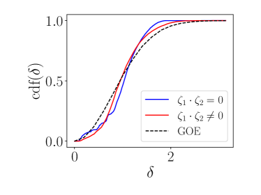
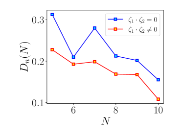
Figure 3: Left Panel : Plot of the peak level spacing statistics CDF of the amplitude with $\zeta_{1}\cdot\zeta_{2}=0$, $\zeta_{1}\cdot\zeta_{2}\neq 0$ and GOE random matrix statistics. Right Panel : KS statistical distance between the level spacing CDF of the amplitude and GOE, showing that $\zeta_{1}\cdot\zeta_{2}\neq 0$ case is closer to GOE for same values of $N$.

3.1.2 Probing off-diagonal matrix elements in the $HHT$ amplitude

We consider coarse-graining over the two $HES$ states in $\langle{HES_{1}(p_{1},\zeta_{1})T(p_{3})HES_{2}(p_{2},\zeta_{2})}\rangle$. The $|HES\rangle$ states are now taken to be at different levels, neverthless we average over all states at a given level. The information that we infer from this amplitude is the same present in the off-diagonal piece of Eq.(1.3). Fixing off-diagonal row & coloumn, i.e., fixed $N_{i}$ and $N_{j}$, we average over the amplitudes (matrix elements) which relate these two energy levels:

$$|{\langle{\tilde{A}}\rangle}_{ij}| =\text{Avg}_{\chi}\bigg{(}{1\over\Omega(N_{i})\Omega(N_{j})}\,\,\bigg{|}\sum_{\begin{subarray}{c}H_{i}\in\{N_{i}\}\\ H_{j}\in\{N_{j}\}\end{subarray}}{\langle{H_{i}TH_{j}}\rangle\over\sqrt{\langle{H_{i}|H_{i}}\rangle}\sqrt{\langle{H_{j}|H_{j}}\rangle}}\bigg{|}\bigg{)},\quad i\neq j.$$ (3.20)

Note, that after summing over states with fixed $N_{i}$ and $N_{j}$, we have taken an absolute value, hence we compare this with $|e^{-S(\bar{E})/2}f(\omega)R_{ij}|=e^{-S(\bar{E})/2}f(\omega)|R_{ij}|$, where $S(\bar{E})$ denotes the entropy corresponding to the states at average energy between $E_{i}$ and $E_{j}$. The coarse-grained amplitudes still depend on the kinematic variable $\chi$, the final averaging is to get rid of this dependence.

Additionally, we have to work with normalized $|HES\rangle$ states now since we Eq.(1.3) that we compare with, is for normalized states (See Appendix §D). Further, we replace ${|R_{ij}|}$ by its statistical average $1$, and then find $f(\omega)$ from the resulting answer by compensating for the entropic suppression. The entire analysis is numerical, since unlike the large $N$ diagonal case, we are unable to carry out the averaging analytically.

In [34] the authors derived an upper bound on $f(\omega)$ from analyticity of the thermal correlator : ${\rm tr}\left(e^{-\beta H/2}O(t)e^{-\beta H/2}O(0)\right)$, which is given by:

$$|f(\omega)|\leq\exp\left(-\beta|\omega|/4\right).$$ (3.21)

The inverse temperature $\beta$ is the effective thermal temperature which is to be associated with the average of $E_{i},E_{j}$. Since we are computing with strings at the correspondence point, we compare the above bound with $\beta$ given by the Schwarzschild temperature when $GM=\sqrt{\alpha^{\prime}}$. Thus we plug into the r.h.s of Eq.(3.21) $\beta=8\pi GM=8\pi\sqrt{\alpha^{\prime}}\simeq 17.7715$.

It is interesting to note that this is the same coarse-graining as in the case for probing ETH in $c>1$ CFTs for heavy states [51, 52, 53], where the analytical form of $f_{O}(\omega)$ revealed the quasi-normal modes. It will be interesting to understand if the modes of the correspondence point black hole can also be probed.

Numerical details

We fix $N_{1}=11$ corresponding to the rest-mass $=4.47214$ and we keep increasing $N_{2}$, thus probing larger $\omega$ regimes. We probe upto $N_{2}=25$, which corresponds to $\omega$ until $2.45607$. This value of $\omega$ is already pushing the limits of the ETH ansatz, which being a statement of local operator matrix elements only connects states non-extensively different in the system size. The number of computations keep growing exponentially with $N$, for instance in the $N_{1}=11,N_{2}=25$ case we average over $109648$ matrix elements. In Fig.4 we compare the numerically extracted $f(\omega)$ as a function of $\omega$. At $\omega=0$ it starts from a non-zero constant and then after a region of non-monotonicity, steadily decreases exponentially while respecting the bound. Since the bound is sensitive to the number $17.7715$ we interpret this as an evidence of ETH, as expected at the correspondence point.

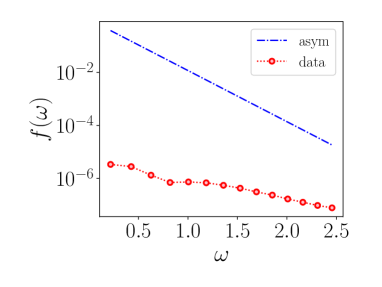
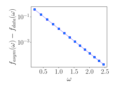
Figure 4: The blue dashed line represents the bound $\exp\left(-\beta|\omega|/4\right)$, where $\beta=17.7715$ is the correspondence point value. The dots are the numerically extracted $f(\omega)$. The plot is on a semi-$\log$ scale for clarity. See text for further details.

4 Computation of $HES_{1}(p_{1},\zeta_{1})+T_{2}(p_{2})\to HES_{3}(p_{3},\zeta_{3})+T_{4}(p_{4})$

In this section we compute the amplitude corresponding to the process as depicted below in Fig.5.

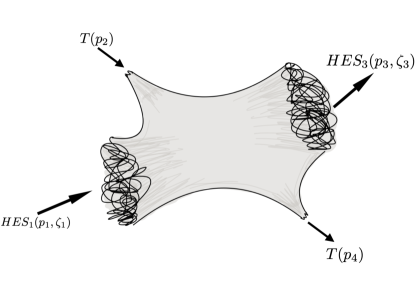
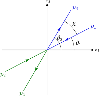
Figure 5: Left Panel : The $2\leftrightarrow 2$ scattering set-up considered. Right Panel : Kinematics indicating the scattering angles, green arrows indicate tachyons, while blue the $HES$.

Since this is a 4 point amplitude, it involves one integral over the cross-ratio. The integrand involves contractions between 4 vertex operators.

$$e^{\cal L}=\bigg{\langle}:\prod_{r_{1}} \left(\sum_{m_{1}}^{r_{1}}{i\over(m_{1}-1)!}\zeta_{1}\cdot\partial^{m_{1}}X_{1}S^{1}_{r_{1}-m_{1}}\right)e^{ip_{1}\cdot X_{1}}::\prod_{r_{3}}\left(\sum_{m_{3}}^{r_{3}}{i\over(m_{3}-1)!}\zeta_{3}\cdot\partial^{m_{3}}X_{3}S^{3}_{r_{3}-m_{3}}\right)$$

$$e^{ip_{3}\cdot X_{3}}::e^{ip_{2}\cdot X_{2}}::e^{ip_{4}\cdot X_{4}}:\bigg{\rangle}$$ (4.1)

Once again, we choose the constituent photons for $|HES_{1}\rangle$ and $|HES_{3}\rangle$ parallel to each other, i.e., $q_{3}=-\gamma q_{1}$. We also naturally have the relations:

$$\zeta_{1}\cdot\zeta_{3} =\lambda_{1}\cdot\lambda_{3},\,\,\ \zeta_{i}\cdot q_{j}=0,\,\,\,\lambda_{i}^{2}=0.$$ (4.2)

Carrying out the possible contractions yield:

$$e^{\cal{L}} =\sum_{k=0}^{\{J_{1},J_{3}\}_{min}}\sum_{\begin{subarray}{c}\{a(k)\}\subset\{r_{1}\}\\ \{b{(k)}\}\subset\{r_{3}\}\\ \text{ordered}\end{subarray}}{1\over k!}\prod_{i=1}^{k}\Bigg{[}\sum_{m_{1},m_{3}=1}^{a_{i},b_{i}}\bigg{\{}{(-1)^{m_{3}+1}(m_{1}+m_{3}-1)!\zeta_{1}.\zeta_{3}\over(m_{1}-1)!(m_{3}-1)!z_{31}^{m_{1}+m_{3}}}\bigg{\}}$$

$$\times S_{a_{i}-m_{1}}\bigg{(}{a_{i}\over s_{1}}\left({q_{1}\cdot p_{3}\over z_{31}^{s_{1}}}+{q_{1}\cdot p_{2}\over z_{21}^{s_{1}}}+{q_{1}\cdot p_{4}\over z_{41}^{s_{1}}}\right)\bigg{)}S_{b_{i}-m_{2}}\bigg{(}{b_{i}\over s_{3}}\bigg{(}{q_{3}\cdot p_{1}\over z_{13}^{s_{3}}}+{q_{3}\cdot p_{2}\over z_{23}^{s_{3}}}+{q_{3}\cdot p_{4}\over z_{43}^{s_{3}}}\bigg{)}\bigg{)}\Bigg{]}$$ (4.3)

$$\times \prod_{l_{1}\in\overline{\{a(k)\}}}\Bigg{[}\sum_{n_{1}=1}^{l_{1}}\bigg{(}{\zeta_{1}\cdot p_{3}\over z_{31}^{n_{1}}}+{\zeta_{1}\cdot p_{2}\over z_{21}^{n_{1}}}+{\zeta_{1}\cdot p_{4}\over z_{41}^{n_{1}}}\bigg{)}S_{l_{1}-n_{1}}\Bigg{]}$$

$$\times \prod_{l_{3}\in\overline{\{b(k)\}}}\Bigg{[}\sum_{n_{3}=1}^{l_{3}}\bigg{(}{\zeta_{3}\cdot p_{1}\over z_{13}^{n_{3}}}+{\zeta_{3}\cdot p_{2}\over z_{23}^{n_{3}}}+{\zeta_{3}\cdot p_{4}\over z_{43}^{n_{3}}}\bigg{)}S_{l_{3}-n_{3}}\Bigg{]}\times\prod_{i<j}z_{ij}^{p_{i}\cdot p_{j}}.$$

Using $SL_{2}$ invariance we fix, $z_{1}=0,z_{2}=x$ and $z_{3}=1$ and $z_{4}=\infty$. The four point amplitude is obtained by integrating over $x$ from $-\infty$ and $\infty$.

$${\cal A}_{4} =\int_{-\infty}^{\infty}{dx\over x^{2}}x^{-p_{1}\cdot p_{3}-p_{3}\cdot p_{2}}(1-x)^{p_{3}\cdot p_{2}}(-x)^{N_{1}+N_{3}}$$

$$\sum_{k=0}^{\{J_{1},J_{3}\}_{min}}\sum_{\begin{subarray}{c}\{a(k)\}\subset\{r_{1}\}\\ \{b{(k)}\}\subset\{r_{3}\}\\ \text{ordered}\end{subarray}}{1\over k!}\prod_{i=1}^{k}\sum_{m_{1},m_{3}=1}^{a_{i},b_{i}}\bigg{[}{(-1)^{m_{3}+1}(m_{3}+m_{1}-1)!\lambda_{1}\cdot\lambda_{3}\over(m_{1}-1)!(m_{3}-1)!}$$

$$\times S_{a_{i}-m_{1}}\bigg{(}{a_{i}\over s_{1}}\left(q_{1}\cdot p_{3}+{q_{1}\cdot p_{2}\over x^{s_{1}}}\right)\bigg{)}\times S_{b_{i}-m_{3}}\bigg{(}{b_{i}\over s_{3}}\bigg{(}(-1)^{s_{3}}q_{3}\cdot p_{1}+{q_{3}\cdot p_{2}\over(x-1)^{s_{3}}}\bigg{)}\bigg{)}\bigg{]}$$

$$\times\prod_{l_{1}\in\overline{\{a(k)\}}}\Bigg{[}\sum_{n_{1}=1}^{l_{1}}\bigg{(}\zeta_{1}\cdot p_{3}+{\zeta_{1}\cdot p_{2}\over x^{n_{1}}}\bigg{)}S_{l_{1}-n_{1}}\bigg{(}{l_{1}\over s_{1}}\left(q_{1}\cdot p_{3}+{q_{1}\cdot p_{2}\over x^{s_{1}}}\right)\bigg{)}\bigg{]}$$

$$\times\prod_{l_{3}\in\overline{\{b(k)\}}}\Bigg{[}\sum_{n_{3}=1}^{l_{3}}\bigg{(}(-1)^{n_{3}}\zeta_{3}\cdot p_{1}+{\zeta_{3}\cdot p_{2}\over(x-1)^{n_{3}}}\bigg{)}S_{l_{3}-m_{3}}\bigg{(}{l_{3}\over s_{3}}\bigg{(}(-1)^{s_{3}}q_{3}\cdot p_{1}+{q_{3}\cdot p_{2}\over(x-1)^{s_{3}}}\bigg{)}\bigg{)}\bigg{]}$$ (4.4)

If we choose kinematics such that $q_{i}\cdot p_{2}=0$ as well as $\zeta_{i}\cdot p_{2}=0$, then we have:

$${\cal A}_{4} =(-1)^{N_{1}+N_{3}}\int x^{N_{1}+N_{3}-2-p_{1}\cdot p_{3}-p_{3}\cdot p_{2}}(1-x)^{p_{3}\cdot p_{2}}$$

$$\sum_{k=0}^{\{J_{1},J_{3}\}_{min}}\sum_{\begin{subarray}{c}\{a(k)\}\subset\{r_{1}\}\\ \{b{(k)}\}\subset\{r_{3}\}\\ \text{ordered}\end{subarray}}{1\over k!}\prod_{i=1}^{k}\sum_{m_{1},m_{3}=1}^{a_{i},b_{i}}\bigg{[}{(-1)^{m_{3}+1}(m_{3}+m_{1}-1)!\lambda_{1}\cdot\lambda_{3}\over(m_{1}-1)!(m_{3}-1)!}$$

$$\times S_{a_{i}-m_{1}}\bigg{(}{a_{i}\over s_{1}}\left(q_{1}\cdot p_{3}\right)\bigg{)}\times S_{b_{i}-m_{3}}\bigg{(}{b_{i}\over s_{3}}\bigg{(}(-1)^{s_{3}}q_{3}\cdot p_{1}\bigg{)}\bigg{)}\bigg{]}$$

$$\times\prod_{l_{1}\in\overline{\{a(k)\}}}\Bigg{[}\sum_{n_{1}=1}^{l_{1}}\bigg{(}\zeta_{1}\cdot p_{3}\bigg{)}S_{l_{1}-n_{1}}\bigg{(}{l_{1}\over s_{1}}\left(q_{1}\cdot p_{3}\right)\bigg{)}\bigg{]}$$

$$\times\prod_{l_{3}\in\overline{\{b(k)\}}}\Bigg{[}\sum_{n_{3}=1}^{l_{3}}\bigg{(}(-1)^{n_{3}}\zeta_{3}\cdot p_{1}\bigg{)}S_{l_{3}-m_{3}}\bigg{(}{l_{3}\over s_{3}}\bigg{(}(-1)^{s_{3}}q_{3}\cdot p_{1}\bigg{)}\bigg{)}\bigg{]}$$ (4.5)

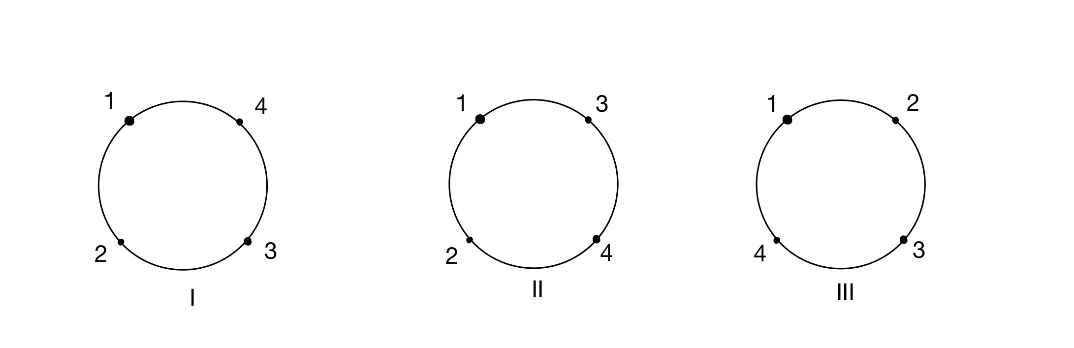
Figure 6: The process can happen in 3 different channels. Interchanging the positions of any two strings will correspond to a different channel. There can be six different diagrams, but $z_{1}=0$, $z_{3}=1$ and $z_{4}=\infty$ is fixed so the other $3$ channels are equivalent to these $3$.

The range of the above integration depends on the choice of channel. The integrals give rise to beta functions. The total amplitude therefore is a sum of different weighted beta functions, corresponding to different channels. In figure 6 the string configurations for different channels are shown. Hence, we write the full amplitude as:

$${\cal A}_{4} =(-1)^{N_{1}+N_{3}}\int x^{N_{1}+N_{3}-2-p_{1}\cdot p_{3}-p_{3}\cdot p_{2}}(1-x)^{p_{3}\cdot p_{2}}\sum_{k=0}^{\{J_{1},J_{3}\}_{min}}\sum_{\begin{subarray}{c}\{a(k)\}\\ \{b{(k)}\}\end{subarray}}{1\over k!}$$

$$\times\Bigg{(}\prod_{i=1}^{k}\bigg{[}\sum_{m_{1},m_{3}=1}^{a_{i},b_{i}}{(-1)^{m_{3}+1}(m_{3}+m_{1}-1)!\lambda_{1}\cdot\lambda_{3}\over(m_{1}-1)!(m_{3}-1)!}S_{a_{i}-m_{1}}\bigg{(}{a_{i}\over s_{1}}q_{1}\cdot p_{3}\bigg{)}S_{b_{i}-m_{3}}\bigg{(}{b_{i}\over s_{3}}(-1)^{s_{3}}q_{3}\cdot p_{1}\bigg{)}\bigg{]}$$

$$~{}~{}~{}~{}\times\prod_{l_{1}\in\overline{\{a(k)\}}}\Bigg{[}\sum_{n_{1}=1}^{l_{1}}\bigg{(}\zeta_{1}\cdot p_{3}\bigg{)}S_{l_{1}-n_{1}}\bigg{(}{l_{1}\over s_{1}}\left(q_{1}\cdot p_{3}\right)\bigg{)}\bigg{]}$$

$$~{}~{}~{}~{}\times\prod_{l_{3}\in\overline{\{b(k)\}}}\Bigg{[}\sum_{n_{3}=1}^{l_{3}}\bigg{(}(-1)^{n_{3}}\zeta_{3}\cdot p_{1}\bigg{)}S_{l_{3}-m_{3}}\bigg{(}{l_{3}\over s_{3}}\bigg{(}(-1)^{s_{3}}q_{3}\cdot p_{1}\bigg{)}\bigg{)}\bigg{]}\Bigg{)}$$

$$=(-1)^{N_{1}+N_{3}}\int x^{N_{1}+N_{3}-2-p_{1}\cdot p_{3}-p_{3}\cdot p_{2}}(1-x)^{p_{3}\cdot p_{2}}$$

$$~{}~{}~{}~{}\times\sum_{k=0}^{min\{J_{1},J_{3}\}}{1\over k!}\sum_{\begin{subarray}{c}\{a(k)\}\\ \{b(k)\}\end{subarray}}\left(\prod_{i=1}^{k}P(a_{i},b_{i})\prod_{l_{1}\in\overline{\{a(k)\}}}Q_{1}(l_{1})\prod_{l_{3}\in\overline{\{b(k)\}}}Q_{3}(l_{3})\right),$$ (4.6)

where $P(a_{i},b_{i})$ is same as that is in equation (2.15), $Q_{1}$ and $Q_{3}$ are given by,

$$Q_{1}(l_{1}) =\sum_{m_{1}=1}^{l_{1}}(\zeta_{1}\cdot p_{3})S_{l_{1}-m_{1}}\bigg{(}-{l_{1}\over s_{1}\gamma}\bigg{)}=(\zeta_{1}\cdot p_{3})(-1)^{l_{1}}\prod_{j_{1}=1}^{l_{1}-1}\bigg{(}{-l_{1}q_{1}\cdot p_{3}-j_{1}\over j_{1}}\bigg{)},$$ (4.7)

$$Q_{3}(l_{2}) =\sum_{m_{2}=1}^{l_{2}}(\zeta_{3}\cdot p_{1})(-1)^{m_{3}}S_{l_{3}-m_{3}}\bigg{(}-{l_{3}(-1)^{s_{3}}\over s_{3}}\gamma\bigg{)}=(\zeta_{3}\cdot p_{1})\prod_{j_{3}=1}^{l_{3}-1}\bigg{(}{-l_{3}q_{3}\cdot p_{1}-j_{3}\over j_{3}}\bigg{)}.$$ (4.8)

Restoring the dependence on $\alpha^{\prime}$ in equation(4) we get,

$${\cal A}_{4} =f_{N_{tot}}(s,t)\sum_{k=0}^{\{J_{1},J_{3}\}_{min}}\sum_{\begin{subarray}{c}\{a(k)\}\\ \{b{(k)}\}\end{subarray}}{1\over k!}\Bigg{(}\prod_{i=1}^{k}\bigg{[}\sum_{m_{1},m_{3}=1}^{a_{i},b_{i}}{(-1)^{m_{3}+1}(m_{3}+m_{1}-1)!\lambda_{1}\cdot\lambda_{3}\over(m_{1}-1)!(m_{3}-1)!}S_{a_{i}-m_{1}}\bigg{(}{2\alpha^{\prime}a_{i}\over s_{1}}q_{1}\cdot p_{3}\bigg{)}$$

$$\times S_{b_{i}-m_{3}}\bigg{(}{2\alpha^{\prime}b_{i}\over s_{3}}(-1)^{s_{3}}q_{3}\cdot p_{1}\bigg{)}\bigg{]}\prod_{l_{1}\in\overline{\{a(k)\}}}\Bigg{[}\sum_{n_{1}=1}^{l_{1}}\bigg{(}\sqrt{2\alpha^{\prime}}\zeta_{1}\cdot p_{3}\bigg{)}S_{l_{1}-n_{1}}\bigg{(}{2\alpha^{\prime}l_{1}\over s_{1}}\left(q_{1}\cdot p_{3}\right)\bigg{)}\bigg{]}$$ (4.9)

$$\times\prod_{l_{3}\in\overline{\{b(k)\}}}\Bigg{[}\sum_{n_{3}=1}^{l_{3}}\bigg{(}(-1)^{n_{3}}\sqrt{2\alpha^{\prime}}\zeta_{3}\cdot p_{1}\bigg{)}S_{l_{3}-m_{3}}\bigg{(}{2\alpha^{\prime}l_{3}\over s_{3}}\bigg{(}(-1)^{s_{3}}q_{3}\cdot p_{1}\bigg{)}\bigg{)}\bigg{]}\Bigg{)},$$

where, $f_{N_{tot}}(s,t)$ is given by the following integral formula that we evaluate using the analytic continuation of beta function as:

$$f_{N_{tot}}(s,t) =(-1)^{N_{tot}}\Bigg{[}\int\limits_{-\infty}^{0}+\int\limits_{0}^{1}+\int\limits_{1}^{+\infty}\Bigg{]}\,\,x^{N_{tot}-2-p_{1}\cdot p_{3}-p_{3}\cdot p_{2}}(1-x)^{-p_{3}\cdot p_{2}}$$

$$=(-1)^{N_{tot}}\Bigg{[}(-1)^{p_{2}\cdot p_{3}}B(3-N_{tot}+p_{1}\cdot p_{3},p_{2}\cdot p_{3}+1)+B(N_{tot}-1-p_{1}\cdot p_{3}-p_{2}\cdot p_{3},p_{2}\cdot p_{3}+1)$$

$$+(-1)^{N_{tot}-1-p_{1}\cdot p_{3}-p_{2}\cdot p_{3}}B(N_{tot}-1-p_{1}\cdot p_{3}-p_{2}\cdot p_{3},3-N_{tot}+p_{1}\cdot p_{3})\Bigg{]},$$ (4.10)

where $N_{tot}=N_{1}+N_{3}$. Here, $s=-(p_{1}+p_{2})^{2}$ and $t=-(p_{1}+p_{3})^{2}$ are the Mandelstam invariants. One can see the structural similarity between Eq.(4.9) and the $HHT$ scattering amplitude, Eq.(2.7) ; thus for the given kinematical choices we find

$${\cal{A}}_{4}(p_{i},\zeta_{i})\sim{\cal{A}}_{3}(p_{i},\zeta_{i})f_{N_{tot}}(p_{i}),$$ (4.11)

i.e., the three point amplitude ${\cal{A}}_{3}$ acts like a dressing of a scalar amplitude to give the required 4 point amplitude with both momenta as well as the polarization vectors.

4.1 Kinematics for $HHTT$ amplitude

Metric signature $(-,+,+\dots+)$. The on-shell condition is $p_{i}^{2}=-M_{i}^{2}$. Furthermore we take all the momenta to be ingoing. We choose the combined COM frame of $H_{1}$ and $T_{2}$. These are ingoing states. The outgoing states are $H_{3}$ and $T_{4}$. HES1 and HES2 have rest mass $\sqrt{2(N_{1}-1)}$ and $\sqrt{2(N_{3}-1)}$ respectively. Let us first write down the parametrizations for the momenta. The list of constraints are,

$$\left(p_{1}\right)^{2} =-M_{1}^{2}=-2(N_{1}-1),\,\,\left(p_{2}\right)^{2}=2,\,\,\left(p_{3}\right)^{2}=-M_{2}^{2}=-2(N_{3}-1),$$

$$\left(p_{4}\right)^{2} =2,\,\,\vec{p_{1}}+\vec{p_{2}}=0=\vec{p_{3}}+\vec{p_{4}},\,\,\,p_{1}+p_{2}+p_{3}+p_{4}=0.$$ (4.12)

Maintaining the constraints we get:

$$p_{1}=\left\{\sqrt{e^{2}+2N_{1}},\sqrt{e^{2}+2}\sin(\theta_{1}),\sqrt{e^{2}+2}\cos(\theta_{1}),0\right\},\,\,p_{2}=\left\{e,-\sqrt{e^{2}+2}\sin(\theta_{1}),-\sqrt{e^{2}+2}\cos(\theta_{1}),0\right\},$$

$$p_{3}=\left\{-\sqrt{d^{2}+2N_{3}},\sqrt{d^{2}+2}\sin(\theta_{2}),\sqrt{d^{2}+2}\cos(\theta_{2}),0\right\},$$

$$p_{4}=\left\{-d,-\sqrt{d^{2}+2}\sin(\theta_{2}),-\sqrt{d^{2}+2}\cos(\theta_{2}),0\right\},$$ (4.13)

where $d={-N_{3}\sqrt{e^{2}+2N_{1}}+N_{1}\sqrt{e^{2}+2N_{1}}+eN_{1}+eN_{3}\over 2N_{1}}$.

The DDF photon momenta are given by :

$$q_{1} =\left\{-{1\over\sqrt{e^{2}+2N_{1}}+e},{e\sin(\theta_{1})\over\sqrt{e^{2}+2}\left(\sqrt{e^{2}+2N_{1}}+e\right)},{e\cos(\theta_{1})\over\sqrt{e^{2}+2}\left(\sqrt{e^{2}+2N_{1}}+e\right)},{\sqrt{2}\over\sqrt{e^{2}+2}\left(\sqrt{e^{2}+2N_{1}}+e\right)}\right\}$$

$$q_{3} =-\gamma q_{1}\;\ \text{where}\;\ \gamma=-{1\over p_{3}\cdot q_{1}}={\sqrt{e^{2}+2}\left(\sqrt{e^{2}+2N_{1}}+e\right)\over\sqrt{e^{2}+2}\sqrt{d^{2}+2N_{3}}-\sqrt{d^{2}+2}e\cos(\theta_{1}-\theta_{2})}.$$ (4.14)

For this particular choice of kinematics, the polarization vectors of the DDF photons must contain an imaginary $5$-th component (to make the polarization vectors to be null-like) :

$$\lambda_{1} ={1\over\sqrt{2}}\{0,\cos\theta_{1},-\sin\theta_{1},0,i\},\lambda_{3}={1\over\sqrt{2}}\{0,\cos\theta_{1},-\sin\theta_{1},0,-i\},\zeta_{1}={1\over\sqrt{2}}\{0,\cos\theta_{1},-\sin\theta_{1},0,i\}$$

$$\zeta_{3} ={1\over\sqrt{2}}\bigg{\{}{\sqrt{(d^{2}+2)(e^{2}+2)}\sin(\theta_{1}-\theta_{2})\over\sqrt{e^{2}+2}\sqrt{d^{2}+2N_{3}}-\sqrt{d^{2}+2}e\cos(\theta_{1}-\theta_{2})},{\sqrt{(e^{2}+2)(d^{2}+2N_{3})}\cos(\theta_{1})-\sqrt{d^{2}+2}e\cos(\theta_{2})\over\sqrt{e^{2}+2}\sqrt{d^{2}+2N_{3}}-\sqrt{d^{2}+2}e\cos(\theta_{1}-\theta_{2})},$$

$$\;\ \;\ \;\ \;\ \;\ \;\ \;\ \;\ {-\sqrt{(e^{2}+2)(d^{2}+2N_{3})}\sin(\theta_{1})+\sqrt{d^{2}+2}e\sin(\theta_{2})\over\sqrt{e^{2}+2}\sqrt{d^{2}+2N_{3}}-\sqrt{d^{2}+2}e\cos(\theta_{1}-\theta_{2})},0,-i\bigg{\}}.$$ (4.15)

If we consider the case $N_{1}=N_{3}=N$, which corresponds to $e=d$, the kinematics and hence the amplitude itself becomes simple:

$$p_{1} =\left\{\sqrt{e^{2}+2N},\sqrt{e^{2}+2}\sin(\theta_{1}),\sqrt{e^{2}+2}\cos\theta_{1},0\right\},\,\,p_{2}=\left\{e,-\sqrt{e^{2}+2}\sin\theta_{1},-\sqrt{e^{2}+2}\cos\theta_{1},0\right\}$$

$$p_{3} =\left\{-\sqrt{e^{2}+2N},\sqrt{e^{2}+2}\sin\theta_{2},\sqrt{e^{2}+2}\cos\theta_{2},0\right\},\,p_{4}=\left\{-e,-\sqrt{e^{2}+2}\sin\theta_{2},-\sqrt{e^{2}+2}\cos\theta_{2},0\right\}$$

$$q_{1} =\left\{-{1\over\sqrt{e^{2}+2N}+e},{e\sin\theta_{1}\over\sqrt{e^{2}+2}\left(\sqrt{e^{2}+2N}+e\right)},{e\cos\theta_{1}\over\sqrt{e^{2}+2}\left(\sqrt{e^{2}+2N}+e\right)},{\sqrt{2}\over\sqrt{e^{2}+2}\left(\sqrt{e^{2}+2N}+e\right)}\right\}$$ (4.16)

$$q_{3} =-\gamma q_{1}\;\ ;\gamma={\sqrt{e^{2}+2N}+e\over\sqrt{e^{2}+2N}-e\cos(\theta_{1}-\theta_{2})}.$$

In this case the amplitude in equation (4) becomes,

$$\mathcal{A}_{4} =f_{2N}(s,t)\sum_{k=0}^{min\{J_{1},J_{3}\}}{1\over k!}\sum_{\begin{subarray}{c}\{a(k)\}\\ \{b(k)\}\end{subarray}}\left(\prod_{i=1}^{k}P(a_{i},b_{i})\prod_{l_{1}\in\overline{\{a(k)\}}}Q_{1}(l_{1})\prod_{l_{3}\in\overline{\{b(k)\}}}Q_{3}(l_{3})\right).$$ (4.17)

Here, $P$, $Q_{1}$ and $Q_{3}$ has the form same as in equation (4), and $\{e,\chi=\theta_{1}-\theta_{2}\}$ are given in terms of Mandelstam invariants $s$ and $t$. These relations and the expression for $\gamma$ are given by:

$$s =\left(\sqrt{e^{2}+2N}+e\right)^{2},\,\,\,t=4\left(e^{2}+2\right)\cos^{2}\left({\chi\over 2}\right),\,\,\,\gamma={\sqrt{e^{2}+2N}+e\over\sqrt{e^{2}+2N}-e\cos\chi}.$$ (4.18)

4.2 Evaluation of $HHTT$ amplitude

When $\zeta_{1}\cdot\zeta_{3}=0$ and $N_{1}=N_{3}=N$, in terms of kinematic parameters $e,\,N,\,\text{ and, }\chi$, the amplitude simplifies:

$$\mathcal{A}_{4} =f_{2N}(s,t)\prod_{\{r_{1}\}}\left(-{\sqrt{e^{2}+2}\sin(\chi)\over\sqrt{2}}(-1)^{r_{1}}\prod_{j_{1}=1}^{r_{1}-1}\bigg{(}{r_{1}/\gamma-j_{1}\over j_{1}}\bigg{)}\right)^{n_{r_{1}}}$$

$$\times\prod_{\{r_{3}\}}\left({\sqrt{e^{2}+2}\sin(\chi)\left(\sqrt{e^{2}+2N}+e\right)\over\sqrt{2}\left(e\cos(\chi)-\sqrt{e^{2}+2N}\right)}\prod_{j_{3}=1}^{r_{3}-1}\bigg{(}{r_{3}\gamma-j_{3}\over j_{3}}\bigg{)}\right)^{n_{r_{3}}}.$$ (4.19)

Where $\gamma$ is given as in equation (4.18), and a particular integer partition of $N_{i}$ is, $N_{i}=\sum_{r_{i}=1}^{N_{i}}r_{i}n_{r_{i}}$ with $r_{i}$’s necessarily distinct integers. Consistency requires that $e>0$, since $T(p_{2})$ is ingoing, see Eq.(4.16). The amplitude can be expressed in terms of the Mandelstam invariant $s=-\left(p_{1}+p_{2}\right)^{2}$ and kinematic angle $\chi=\chi(s,t)$, by plugging in:

$$e ={s-2N\over 2\sqrt{s}},\,\,\,\gamma={2s\over(2N-s)\cos(\chi)+2N+s},$$ (4.20)

$$\cos\chi =-1-{2st\over 8s+(s-2N)^{2}},$$

to obtain:

$$\mathcal{A}_{4} =f_{2N}\left(s,t\right)\prod_{\{r_{1}\}}\left(-\left(\sqrt{{(s-2N)^{2}\over 8s}+1}\right)\sin(\chi)\prod_{j_{1}=1}^{r_{1}-1}\bigg{(}{r_{1}/\gamma-j_{1}\over j_{1}}\bigg{)}\right)^{n_{r_{1}}}$$

$$\times\prod_{\{r_{3}\}}\left(-{s\left(\sqrt{{(s-2N)^{2}\over 2s}+4}\right)\sin(\chi)\over(2N-s)\cos(\chi)+2N+s}\prod_{j_{3}=1}^{r_{3}-1}\bigg{(}{r_{3}\gamma-j_{3}\over j_{3}}\bigg{)}\right)^{n_{r_{3}}}$$ (4.21)

5 $HHTT$ in different regimes and its statistics

In this section we look at various asymptotic regimes where the above amplitude exhibits interesting behaviours. We also demonstrate its chaotic nature in the probe limit, as well as, point out how it realizes a notion of typicality.

5.1 Fixed angle high energy scattering

This is the limit when $s\gg 2N$, and $\chi$ is fixed. The Mandelstam invariant $t$ is also large. The various factors become:

$$f_{2N}(s,\chi) \simeq B\left(-{s\over 2},{s\over 2}\sin^{2}\tfrac{\chi}{2}\right)-e^{-{1\over 2}i\pi s}B\left(-{s\over 2},{s\over 2}\cos^{2}\tfrac{\chi}{2}\right)+e^{{1\over 2}is\pi\sin^{2}({\small{\chi}/{2}})}B\left({s\over 2}\sin^{2}\tfrac{\chi}{2},{s\over 2}\cos^{2}\tfrac{\chi}{2}\right),$$ (5.1)

$$\gamma \sim{1\over\sin^{2}({\chi\over 2})},\,\,\zeta_{1}\cdot p_{3}\sim-{\sqrt{s}\over 2\sqrt{2}}\sin(\chi),\,\,\,\zeta_{3}\cdot p_{1}\sim-\sqrt{{s\over 2}}\cot({\chi\over 2}).$$

The $4$ point amplitude in this limit becomes :

$$\mathcal{A}_{4}^{\text{fixed }\chi} =f_{2N}(s,\chi)\bigg{(}-{\sqrt{s}\over 2\sqrt{2}}\sin\chi\bigg{)}^{J_{1}}\bigg{(}\sqrt{{s\over 2}}\cot\tfrac{\chi}{2}\bigg{)}^{J_{3}}$$

$$\times\prod_{\{r_{3}\}}\left({\Gamma(r_{3}\csc^{2}\tfrac{\chi}{2})\Gamma(r_{3}-r_{3}\csc^{2}\tfrac{\chi}{2})\over\Gamma(r_{3})}\sin\left(\pi r_{3}\csc^{2}\tfrac{\chi}{2}\right)\right)^{n_{r_{3}}}$$ (5.2)

$$\times\prod_{\{r_{1}\}}\left((-1)^{r_{1}}{\Gamma(r_{1}-r_{1}\cos^{2}\tfrac{\chi}{2})\Gamma(r_{1}\cos^{2}\tfrac{\chi}{2})\over\Gamma(r_{1})}\sin\left(\pi r_{1}\cos^{2}\tfrac{\chi}{2}\right)\right)^{n_{r_{1}}}.$$

Note, that when $N\gg 1$, this limit also satisfies the condition $s\gg|t|$ for all values of the scattering angle $\chi$. This however is still not the Regge limit where forward scattering dominates. In [30] the $HTTT$ amplitude was also computed in this limit. In their set-up, two tachyons come in head-on and the resulting scattering angle is $\theta$ :

$$\mathcal{A^{\prime}}_{4}^{\text{fixed }\theta} =f^{\prime}_{N}(s,\theta)\bigg{(}-\sqrt{s}(1-\tfrac{1}{2}\sin\theta)\bigg{)}^{J}\prod_{\{r\}}\bigg{(}{\Gamma(r\sin\theta)\Gamma(r-r\sin\theta)\over\Gamma(r)}\sin\left(\pi r\sin\theta\right)\bigg{)}^{n_{r}}.$$ (5.3)

The overall $s$ dependent factor in the forward scattering limit for $HTTT$ is $\left(\sqrt{s}\right)^{J}$ whereas, for $HHTT$ it is $\left(\sqrt{s}\right)^{J_{1}+J_{3}}$. Furthermore the structure of the factors appearing within the product is also similar. The dressing factor doubles in the $HHTT$ case, corresponding to the two $|HES\rangle$ states.

5.2 Regge limit

The Regge limit corresponds to $s\gg|t|$ irrespective of any bound on the parameter $N$. In Regge limit the various ingredients in the amplitude, Eq.(4.21) behaves as:

$$\gamma \simeq 1+\mathcal{O}\left({|t|\over s}\right),\,\,f_{2N}(s,t)\simeq{\cal{A}}_{Ven}^{Regge}=\Gamma(-\tfrac{t}{2}-1)s^{\tfrac{t}{2}+1},\,\,\zeta_{1}\cdot p_{3}\simeq\zeta_{3}\cdot p_{1}\simeq\sqrt{{|t|\over 2}},$$ (5.4)

$$\mathcal{A}_{4}^{Regge} \simeq{\cal{A}}_{Ven}^{Regge}\prod_{r_{1}}((-1)^{r_{1}}\zeta_{1}\cdot p_{3})^{n_{r_{1}}}\prod_{r_{3}}(\zeta_{3}\cdot p_{1})^{n_{r_{3}}}=(-1)^{N}\Gamma(-\tfrac{t}{2}-1)s^{\tfrac{t}{2}+1}\left({|t|\over 2}\right)^{{J_{1}+J_{3}\over 2}}.$$

The exponent is consistent with the expected linear Regge trajectory.

5.3 Probe limit : $\alpha^{\prime}s\sim N\gg 1$

In case of classical scattering processes, the fractal structure in the scattering data is considered to be a marker of chaos. For example, one may consider a low-energy particle being scattered by some potential and plot the angle $\theta$ of the outgoing particle (i.e, the output parameter) as a function of the incoming impact parameter $b$. If the scattering is a chaotic one, then $\theta(b)$ will have regions in $b$ where the data will be speckled (i.e, regions of dense fluctuations). As one zooms into these dense regions, again self similar dense scattering data appears. Existence of this kind of fractal structure in the scattering data are considered as the marker of transient chaos [54]. In [31] such a set-up was investigated in the context of $HHTT$ scattering where the outgoing angle for a fixed ingoing one: $\theta^{\prime}(\theta)$ was selected from the largest residue in the amplitude at fixed $s$. The strategy was implemented for fixed partitionings of $|HES\rangle$ states, hence there was no coarse-graining involved. Our strategy however is to implement coarse-graining, in order to make the notions of chaos and thermalizations emergent in the many-body context.

The classical analysis demands that we consider scattering a light particle by some potential. In terms of the 4-point $HHTT$ scattering, this can be interpreted as a low-energy string scattering against the $|HES\rangle$ at much higher energies. When $s\,\alpha^{\prime}$ is of order $N$ which is taken to be large, this corresponds to $N\gg\alpha^{\prime}e^{2}$. Here $t$ is fixed via the fixed scattering angle $\chi$, while we take the large $s$ limit. This means that the tachyon probe comes in with very low energy ($p_{2}^{0}=e$) compared to the $|HES\rangle$ target. For $\alpha=\tfrac{1}{2}$ and $N_{1}=N_{3}=N$ the Veneziano amplitude portion behaves as,

$$f_{2N}(s,t) =\int\limits_{-\infty}^{+\infty}x^{2N-2-p_{1}\cdot p_{3}-p_{3}\cdot p_{2}}(1-x)^{p_{3}\cdot p_{2}}\sim-{4(1+2\cos\chi)\over s-2N}+{\cal{O}}\left((s-2N)^{0}\right).$$ (5.5)

The $HHTT$ amplitude has a simple pole at $s\to N/\alpha^{\prime}$, whose residue is:

• For $\zeta_{1}\cdot\zeta_{3}=0$,

  $$\mathcal{A}_{4}^{\text{res}}|_{s\to 2N}\sim(1+2\cos\chi)(-\sin\chi)^{J_{1}+J_{3}}(-1)^{N},$$ (5.6)

• For $\zeta_{1}\cdot\zeta_{3}\neq 0$,

  $$\mathcal{A}_{4}^{\text{res}}|_{s\to 2N}\sim(1+2\cos\chi)(-\sin\chi)^{J_{1}+J_{3}}(-1)^{N}\sum_{k=0}^{\text{min}\{J_{1},J_{3}\}}{(\sin\chi)^{-2k}\over k!}\sum_{\begin{subarray}{c}\{a(k)\}\\ \{b(k)\}\end{subarray}}\prod_{i=1}^{k}\delta_{a_{i},b_{i}}(-a_{i}).$$ (5.7)

The peak statistics of both of these residues, show level repulsion (see Fig. 7), thus highlighting the inherent chaotic nature of the scattering in the probe limit. However we do not find any randomness with the position of the largest residue within the $|HES\rangle$ ensemble. In this sense our results are consistent with absence of transient chaos if we focus only on the largest residue as in [31].

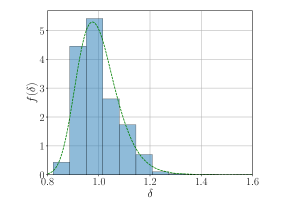
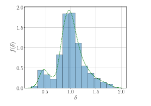
Figure 7: Nearest level spacing distribution of the residue $\mathcal{A}_{4}^{\text{res}}$ at probe limit for two cases. Left Panel: $\zeta_{1}\cdot\zeta_{3}=0$ and $N=20$, Right Panel: $\zeta_{1}\cdot\zeta_{3}\neq 0$ and $N=10$. Both of these show level repulsion.

The $\zeta_{1}\cdot\zeta_{3}=0$ answer in Eq.(5.6) is very similar to the three point amplitudes $HHT$ we got for large $N$. So the full average of the amplitude is given in the same way as equation (3.9) :

$$\langle\mathcal{A}_{4}\rangle_{F} \simeq-{4(1+2\cos\chi)\over s-2N}\exp\Bigg{[}4\sqrt{N}\bigg{(}\sqrt{\text{Li}_{2}(-\sin\chi)}-{\pi\over\sqrt{6}}\bigg{)}\Bigg{]}.$$ (5.8)

Similar to the discussion of §3 we can also consider the diagonal part:

$$\langle\mathcal{A}_{4}\rangle_{D} \simeq-{4(1+2\cos\chi)\over s-2N}\exp\Bigg{[}2\sqrt{N}\bigg{(}\sqrt{\text{Li}_{2}(\sin^{2}\chi)}-{\pi\over\sqrt{6}}\bigg{)}\Bigg{]}.$$ (5.9)

Therefore the probe limit is also sensitive to the thermal scales of the problem just as the three point function is.

5.4 Numerically probing typicality

In this subsection we study the different microstate-channel contributions in the $HHTT$ S-matrix amplitudes, Eq.(4.21). We consider the case $N_{1}=N=N_{3}$, and investigate numerically the partition dependences. We define the relevant part of the amplitude as:

$$\tilde{\mathcal{A}}_{4}(\mathcal{P}_{i},\mathcal{P}_{j})= \prod_{r_{1}\in\mathcal{P}_{i}}\left(-\left(\sqrt{{(s-2N)^{2}\over 8s}+1}\right)\sin(\chi)\prod_{j_{1}=1}^{r_{1}-1}\bigg{(}{r_{1}/\gamma-j_{1}\over j_{1}}\bigg{)}\right)$$

$$\times\prod_{r_{3}\in\mathcal{P}_{j}}\left(-{s\left(\sqrt{{(s-2N)^{2}\over 2s}+4}\right)\sin(\chi)\over(2N-s)\cos(\chi)+2N+s}\prod_{j_{3}=1}^{r_{3}-1}\bigg{(}{r_{3}\gamma-j_{3}\over j_{3}}\bigg{)}\right)$$ (5.10)

where $\mathcal{P}_{i}$ and $\mathcal{P}_{j}$ are partitions of $N_{1}$ and $N_{3}$ respectively; the partitions can contain repeated elements (hence the absence of $n_{r_{1}}$ and $n_{r_{3}}$ factors in the expression).

Here we study $\tilde{\mathcal{A}}_{4}(\mathcal{P}_{i},\mathcal{P}_{j})$ for $N=5$ case for a range $s\gtrsim 2N$ to $s\gg 2N$. Here the partitions are denoted as $\mathcal{P}_{1}\equiv\{5\},~{}\mathcal{P}_{2}\equiv\{4,1\},~{}\mathcal{P}_{3}\equiv\{3,2\},~{}\mathcal{P}_{4}\equiv\{3,1,1\},~{}\mathcal{P}_{5}\equiv\{2,2,1\},~{}\mathcal{P}_{6}\equiv\{2,1,1,1\},~{}\mathcal{P}_{7}\equiv\{1,1,1,1,1\}$.

Below in Fig.8 and in Fig.9 the S-matrix absolute amplitude is plotted for increasing values of $s$ starting from $s\gtrsim 2N$ for $\zeta_{1}\cdot\zeta_{3}=0$ and $\zeta_{1}\cdot\zeta_{3}\neq 0$ respectively. At $s\simeq 2N$, $\tilde{\mathcal{A}}_{4}(\mathcal{P}_{1},\mathcal{P}_{1})$ has the highest amplitude. For $\zeta_{1}\cdot\zeta_{3}=0$ case, with increasing $s$ the amplitude matrix profile shifts smoothly and for $s\gtrsim 2N$ the maxima saturates at $\tilde{\mathcal{A}}_{4}(\mathcal{P}_{1},\mathcal{P}_{7})$. For even greater values of $s$ the maximum amplitude shifts smoothly to $\tilde{\mathcal{A}}_{4}(\mathcal{P}_{7},\mathcal{P}_{7})$ for $s\gg 2N$. This feature continues to hold independent of $\chi$ as well as $N$.

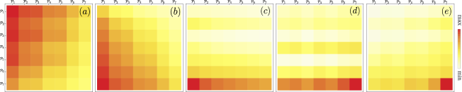
Figure 8: $|\tilde{\mathcal{A}}_{4}(N=5,s,\chi=1.2)|$ for the case $\zeta_{1}\cdot\zeta_{3}=0$, plotted for the $s$ values (a) 10.137, (b) 11.1507, (c) 21.2878, (d) 44.6031, (e) 204.769. Column and row partitions correspond to partitions of $N_{1}$ and $N_{2}$ respectively. With increasing $s$ the maximum amplitude moves smoothly from $\tilde{\mathcal{A}}_{4}(\mathcal{P}_{1},\mathcal{P}_{1})$ in (a) to $\tilde{\mathcal{A}}_{4}(\mathcal{P}_{1},\mathcal{P}_{7})$ in (c). For larger $s$ the maxima smoothly saturates to $\tilde{\mathcal{A}}_{4}(\mathcal{P}_{7},\mathcal{P}_{7})$.

The dominant microstate channels can be explained from Eq.(5.4) in various regimes. At $s\simeq 2N$, one can expand $\tilde{\mathcal{A}}_{4}$ to obtain (see Eq.(5.6)):

$$\tilde{\mathcal{A}}_{4}(\mathcal{P}_{i},\mathcal{P}_{j})\sim\left(-\sin(\chi)\right)^{J_{1}+J_{3}}(-1)^{N}$$ (5.11)

where, $N=\sum_{r}rn_{r},~{}~{}~{}J=\sum_{r}n_{r}$. Now, since we have $0\leq\sin(\chi)\leq 1$, $|\tilde{\mathcal{A}}_{4}|$ is maximum when $(J_{1}+J_{3})$ is minimum. As $\mathcal{P}_{1}$ has $J=\min J=1$, thus at $s\simeq 2N$ the $\tilde{\mathcal{A}}_{4}(\mathcal{P}_{1},\mathcal{P}_{1})$ component dominates. For $s\gtrsim 2N$, we expand Eq.(5.4) around $s=2N(1+\epsilon)$ with $\epsilon>0$ and keep till linear order in $\epsilon$. In this limit individual factors in (5.4) become:

$$\gamma\simeq 1+{\epsilon\over 2}(\cos(\chi)+1)\equiv 1+\epsilon a;~{}\zeta_{1}.p_{3}\simeq-\sin(\chi);~{}\zeta_{3}.p_{1}\simeq-\sin(\chi)(1+\epsilon a)$$

The two sub-products appearing in Eq.(5.4) reduce to:

$$\prod_{j_{1}=1}^{r_{1}-1} \simeq 1-{\epsilon\over 2}(1+\cos(\chi))(\gamma_{E}+\psi(r_{1})),\,\,\,\prod_{j_{2}=1}^{r_{2}-1}\simeq 1+{\epsilon\over 2}(1+\cos(\chi))(\gamma_{E}+\psi(r_{2})),$$

where, $\gamma_{E}$ denotes the Euler number, $\psi(r)=\Gamma^{\prime}(r)/\Gamma(r)$ is the digamma function. Hence, upto linear order in $\epsilon$ we obtain:

$$\tilde{\mathcal{A}}_{4}(\mathcal{P}_{i},\mathcal{P}_{j}) \sim\prod_{\begin{subarray}{c}r_{1}\in\mathcal{P}_{i}\\ r_{1}\text{ distinct}\end{subarray}}\left(-\sin(\chi)\left(1-{\epsilon\over 2}(1+\cos(\chi))(\gamma_{E}+\psi(r_{1}))\right)\right)^{n_{r_{1}}}$$

$$\prod_{\begin{subarray}{c}r_{2}\in\mathcal{P}_{j}\\ r_{2}\text{ distinct}\end{subarray}}\left(-\sin(\chi)\left(1+{\epsilon\over 2}(1+\cos(\chi))(1+\gamma_{E}+\psi(r_{2}))\right)\right)^{n_{r_{2}}}.$$ (5.12)

The magnitude of the first product is always less than $1$ whereas for the second it is larger than $1$. Thus for typical values of $\chi$, $\tilde{\mathcal{A}}_{4}(s\gtrsim 2N)$ maximizes when $J_{1}=\min J_{1}$ and $J_{2}=\max J_{2}$; so the asymmetric corner channel $\tilde{\mathcal{A}}_{4}(\mathcal{P}_{1},\mathcal{P}_{7})$ dominates the scattering process. Next, for $s\gg 2N$, from Eq.(5.2) we have for non-zero values of $\chi$: $\tilde{\mathcal{A}}_{4}(\mathcal{P}_{i},\mathcal{P}_{j})\sim\left(\sqrt{s}\right)^{J_{1}+J_{2}}$. So the component with $J_{1}=\max J_{1}$ and $J_{2}=\max J_{2}$ dominates. Thus in case of $N=5$, for $s\gg 2N$ the $\tilde{\mathcal{A}}_{4}(\mathcal{P}_{7},\mathcal{P}_{7})$ has the maximum amplitude. Lastly, for the $\chi=0$, the $\chi$ dependent part in Eq.(5.2) seems to be diverging because of the $\cot(\chi/2)$ factor. But one can take the $\chi\to 0$ limit carefully: $\gamma\xrightarrow{\chi\to 0,~{}s\gg 2N}{s\over 2N};\,\,~{}\zeta_{1}.p_{3}\xrightarrow{\chi\to 0,~{}s\gg 2N}{\chi\sqrt{s}\over 2\sqrt{2}};\,\,~{}\zeta_{3}.p_{1}\xrightarrow{\chi\to 0,~{}s\gg 2N}{\chi s^{3/2}\over 4\sqrt{2}N}$. Hence the product factors simplify to:

$$\prod_{j_{1}=1}^{r_{1}-1}\left({r_{1}/\gamma-j_{1}\over j_{1}}\right) \xrightarrow{s\gg 2N}1,\,\,\,\prod_{j_{2}=1}^{r_{2}-1}\left({r_{2}\gamma-j_{2}\over j_{2}}\right)\simeq\xrightarrow{s\gg 2N}{1\over\Gamma(r_{2})}$$

Therefore in the limit $s\gg 2N,\chi\to 0$ :

$$\tilde{\mathcal{A}}_{4}(\mathcal{P}_{i},\mathcal{P}_{j}) \sim\prod_{\begin{subarray}{c}r_{1}\in\mathcal{P}_{i}\\ r_{1}\text{ distinct}\end{subarray}}\left({\chi\sqrt{s}\over 2\sqrt{2}}\right)^{n_{r_{1}}}\prod_{\begin{subarray}{c}r_{2}\in\mathcal{P}_{j}\\ r_{2}\text{ distinct}\end{subarray}}\left({\chi s^{3/2}\over 4\sqrt{2}N}{1\over\Gamma(r_{2})}\right)^{n_{r_{2}}}\sim s^{J_{1}/2}s^{3J_{2}/2}$$ (5.13)

Again this is maximum for $J_{1}=\max J_{1}$ and $J_{2}=\max J_{2}$; thus the $\tilde{\mathcal{A}}_{4}(\mathcal{P}_{7},\mathcal{P}_{7})$ dominates for all values of $\chi$ when $s\gg 2N$.

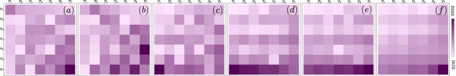
Figure 9: $|\tilde{\mathcal{A}}_{4}(N=5,s,\chi=1.2)|$ for the case $\zeta_{1}\cdot\zeta_{3}\neq 0$, plotted for the $s$ values (a) 10.137, (b) 15.2056, (c) 34.466, (d) 66.9048, (e) 93.2612, (f) 204.769. Column and row partitions correspond to partitions of $N_{1}$ and $N_{2}$ respectively. For $s\gtrsim 2N$, the amplitude is scattered throughout the partitions with no smooth transition. For larger $s$ the maxima smoothly saturates from $\tilde{\mathcal{A}}_{4}(\mathcal{P}_{1},\mathcal{P}_{7})$ in (d) to $\tilde{\mathcal{A}}_{4}(\mathcal{P}_{7},\mathcal{P}_{7})$ in (f).

Since the 4 point scattering amplitude has a dressing factor similar to the $HHT$ amplitude, Eq.(4.11), the thermal characteristics of the three point amplitude get inherited into the four point function as well. It is then natural to consider the centre-of-mass energy scale $s$ to give rise to an effective temperature in this context. Our numerical observations indicate that at higher temperatures (large $s$) the microstate channel which dominates is the one made out of small integer partitions. We point out that this typicality is expected for the $|HES\rangle$ states which can be represented by integer partitionings or Young tableaux. Young tableaux follows the Bose-Einstein distribution [38]. Excited descendants in 2D conformal field theories are also similarly labelled, and the same fact was used to establish typicality in [37] by investigating stress-tensor correlators. Given, the Bose-Einstein distribution, the average occupation number $n_{r}$ of mode number $r$ at inverse temperature $\beta$, for a system of size $L$ is:

$$\langle{n_{r}}\rangle_{\beta} ={1\over e^{2\pi\beta/Lr}-1}\xrightarrow{\beta/L\ll 1}{L\over 2\pi\beta r}.$$ (5.14)

Hence at high temperatures the lowest mode number : $r=1$ are dominantly occupied. This is consistent with the observed channel dominance at large $s$.

6 $HES$ form factor

According to our kinematic choice the process we want to study is

$$HES_{1}(p_{1})+T_{2}(p_{2})\to HES_{3}(p_{3})+T_{4}(p_{4}).$$ (6.1)

In QFT The elctromagnetic form factor of particle $1$ (which is identical to particle $3$) is obtained from the given process in Fig. 10. In the diagram the process is a QED interaction. The form factor of particle $2$ (which is identical to particle $4$) is known. Similarly if the form factor of a tachyon is known, then the form factor of a HES state can be calculated from a similar vertex. In our case string $1$ and $3$ are HES and rest are tachyons. Hence we must consider the process in channel II in figure 6. A schematic diagram of the string interactiion is showed in Fig. 10.

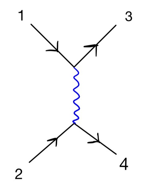
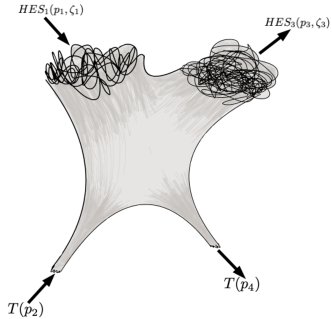
Figure 10: Left Panel : A QED process where the external particles are fermions and the internal propagator is a photon propagator. Right Panel : The string interaction vertex at tree level. For the calculation of the form factor of HES the above configuration should be considered.

The momenta of the states are taken so that the $p_{1},p_{2}$ are ingoing states(energy is positive) and $p_{3},p_{4}$ are outgoing states (therefore energy is negative in accordance with our conventions). To study the form factor of $|HES\rangle$ states we get contribution from a vertex which can be represented by the diagram in Fig.10. Hence the range of the integral in equation (4) would be $x\in(-\infty,0)$. In that limit the integral part of the equation (4) becomes,

$$(-1)^{N_{1}+N_{3}-1}\int_{-\infty}^{0}dxx^{N_{1}+N_{3}-2-p_{1}\cdot p_{3}-p_{2}\cdot p_{3}}(1-x)^{p_{2}\cdot p_{3}}$$

$$=(-1)^{p_{1}\cdot p_{3}+p_{2}\cdot p_{3}}{\Gamma(p_{1}\cdot p_{3}-N_{1}-N_{3}+1)\Gamma(-p_{1}\cdot p_{3}-p_{2}\cdot p_{3}+N_{1}+N_{3}-1)\over\Gamma(-p_{2}\cdot p_{3})}$$

$$=(-1)^{p_{1}\cdot p_{3}+p_{2}\cdot p_{3}}{\Gamma(-1+N-s/2)\Gamma(-1-t/2)\over\Gamma(-2+N-s/2-t/2)}\text{ if }N_{1}=N_{3}=N$$

$$\sim(-1)^{N+{s\over 2}+{t\over 2}}\left({s\over 2}\right)^{1+{t\over 2}}\Gamma(-1-{t\over 2})\text{ in Regge limit}$$ (6.2)

The $t$-channel amplitude with $\zeta_{1}\cdot\zeta_{3}=0$ and $N_{1}=N_{3}=N$ is given by,

$${\cal{A}}_{t} =(-1)^{p_{1}\cdot p_{3}+p_{2}\cdot p_{3}}B(1+p_{1}\cdot p_{3}-N_{1}-N_{3},N_{1}+N_{3}-1-(p_{1}+p_{2})\cdot p_{3})$$

$$\prod_{\{r_{1}\}}\left(\zeta_{1}\cdot p_{3}(-1)^{r_{1}}\prod_{j_{1}=1}^{r_{1}-1}{r_{1}/\gamma-j_{1}\over j_{1}}\right)^{n_{r_{1}}}\prod_{\{r_{3}\}}\left(\zeta_{3}\cdot p_{1}\prod_{j_{3}=1}^{r_{3}-1}{r_{3}\gamma-j_{3}\over j_{3}}\right)^{n_{r_{3}}},$$

$$=(-1)^{N+{s\over 2}}{\Gamma(-1+N-{s\over 2})\Gamma(-1-{t\over 2})\over\Gamma(-2+N-{s\over 2}-{t\over 2})}\prod_{\{r_{1}\}}\left({\sqrt{-t}\sqrt{(s-2N)^{2}+st+8s}\over\sqrt{2}\sqrt{(s-2N)^{2}+8s}}(-1)^{r_{1}}\prod_{j_{1}=1}^{r_{1}-1}{r_{1}/\gamma-j_{1}\over j_{1}}\right)^{n_{r_{1}}}$$

$$\prod_{\{r_{3}\}} \left({\sqrt{-t}\sqrt{(s-2N)^{2}+8s}\sqrt{(s-2N)^{2}+st+8s}\over\sqrt{2}\left((s-2N)^{2}-2Nt+st+8s\right)}\prod_{j_{3}=1}^{r_{3}-1}{r_{3}\gamma-j_{3}\over j_{3}}\right)^{n_{r_{3}}}.$$ (6.3)

In the above expression

$$\gamma={(s-2N)^{2}+8s\over 4N^{2}-2N(2s+t)+s(s+t+8)}.$$

We interpret Mandelstam variable $t$ as the transfer momentum at a $3$ point vertex, similar to QFT vertices i.e. $t=-Q^{2}$, where $Q=p_{1}+p_{3}$. In Regge limit (when $s\gg|t|=Q^{2}$) we have:

$$\gamma =1+{Q^{2}\over s}+O\left(s^{-2}\right),\,\,\zeta_{1}\cdot p_{3}={Q\over\sqrt{2}}-{Q^{3}\over\left(2\sqrt{2}\right)s}+O\left(s^{-2}\right),\,\,\zeta_{3}\cdot p_{1} ={Q\over\sqrt{2}}+{Q^{3}\over\left(2\sqrt{2}\right)s}+O\left(s^{-2}\right).$$ (6.4)

Hence the amplitude simplifies to:

$$\mathcal{A} \sim(-1)^{N+{s\over 2}+{t\over 2}}\left({s\over 2}\right)^{1+{t\over 2}}\Gamma(-1-{t\over 2})\prod_{\{r_{1}\}}\left({Q\over\sqrt{2}}(-1)^{r_{1}}\right)^{n_{r_{1}}}\prod_{\{r_{3}\}}\left({Q\over\sqrt{2}}\right)^{n_{r_{3}}}$$ (6.5)

$$\mathcal{A} \sim(-1)^{{s\over 2}+{t\over 2}}\left({s\over 2}\right)^{1+{t\over 2}}\Gamma(-1-{t\over 2})\prod_{\{r_{1}\}}\left({Q\over\sqrt{2}}\right)^{n_{r_{1}}}\prod_{\{r_{3}\}}\left({Q\over\sqrt{2}}\right)^{n_{r_{3}}}$$ (6.6)

At small momentum transfer $Q^{2}\to 0$, there is a $Q^{2}=0$ pole in the amplitude with coefficient given as below,

$$\mathcal{A} \sim{1\over Q^{2}}(-1)^{{s-Q^{2}\over 2}}s\exp[-{Q^{2}\over 2}\log({s\over 2})]\left({Q\over\sqrt{2}}\right)^{J_{1}+J_{3}}\sim{1\over Q^{2}}\mathcal{F}_{c}(Q^{2})\mathcal{F}_{N,\{n_{r_{1}}\},\{n_{r_{3}}\}}(Q^{2}).$$ (6.7)

In the above expression,

$$\mathcal{F}_{c}(Q^{2})=s\exp[-{Q^{2}\over 2}\log({s\over 2})]$$

is the tachyon vertex form factor and $\mathcal{F}_{N,\{n_{r_{1}}\},\{n_{r_{3}}\}}(Q^{2})=(-1)^{{s-Q^{2}\over 2}}\left({Q\over\sqrt{2}}\right)^{J_{1}+J_{3}}$ is the form factor for the $HES-HES$-massless intermediate particle vertex form factor. This is the leading order behavior of the quantity which depends on the partition of the $|HES\rangle$ state we are choosing. The average form factor can be obtained by summing over the final microstates at level $N_{3}$ and by averaging over the initial microstates at level $N_{1}$ [39] :

$$\langle|\mathcal{A}|^{2}\rangle ={1\over\Omega(N_{1})}\sum_{\{n_{r_{1}}\},\{n_{r_{3}}\}}{|\mathcal{A}|^{2}}={1\over Q^{4}}|\mathcal{F}_{c}(Q^{2})|^{2}|\mathcal{F}_{N}(Q^{2})|^{2}$$ (6.8)

We consider elastic limit with $N_{1}=N_{3}=N$. For all possible in states and out states, the average $4$ point amplitude becomes:

$$\langle{|{\cal A}|^{2}}\rangle ={1\over\Omega(N)}\sum_{\begin{subarray}{c}\{n_{r_{1}}\}\\ \{n_{r_{3}}\}\end{subarray}}\oint d\beta_{1}d\beta_{3}\,\,e^{\beta_{1}N+\beta_{3}N}e^{-\beta_{1}\sum_{r_{1}}r_{1}n_{r_{1}}}e^{-\beta_{3}\sum_{r_{3}}r_{3}n_{r_{3}}}|\mathcal{A}_{(\{r_{1}\},\{r_{3}\},\zeta_{1}\cdot\zeta_{3}=0)}|^{2}$$ (6.9)

In the Regge limit of small momenta transfer we find using Eq.(6.7) :

$$\begin{split}\langle{|{\cal A}|^{2}}\rangle&={s^{2}\exp[Q^{2}\log({s\over 2})]\over\Omega(N)\,Q^{4}}\sum_{\begin{subarray}{c}n_{r_{1}}=0\\ n_{r_{3}}=0\end{subarray}}^{\infty}\oint d\beta_{1}d\beta_{3}\,\,e^{\beta_{i}N}\prod_{r_{1}=1}^{\infty}e^{-\beta_{1}r_{1}n_{r_{1}}}\left({Q^{2}\over 2}\right)^{n_{r_{1}}}\prod_{r_{3}=1}^{\infty}e^{-\beta_{3}r_{3}n_{r_{3}}}\left({Q^{2}\over 2}\right)^{n_{r_{3}}}\\ &={s^{2}\exp[Q^{2}\log({s\over 2})]\over\Omega(N)\,Q^{4}}\oint d\beta_{1}d\beta_{3}\,\,e^{\beta_{i}N}\prod\limits_{r_{1}\in\{N\}}{1\over 1-{Q^{2}\over 2}e^{-\beta_{1}r_{1}}}\prod\limits_{r_{3}\in\{N\}}{1\over 1-{Q^{2}\over 2}e^{-\beta_{3}r_{3}}}.\end{split}$$ (6.10)

We proceed to evaluate the $\beta_{1},\beta_{3}$ integrals using saddle point :

$$\begin{split}\langle{|{\cal A}|^{2}}\rangle&={s^{2}\exp[Q^{2}\log({s\over 2})]\over Q^{4}}\exp\left[4\sqrt{N}\bigg{\{}\sqrt{\text{Li}_{2}{Q^{2}\over 2})}-{\pi\over 2\sqrt{6}}\bigg{\}}\right]\end{split}$$ (6.11)

Therefore we identify the effective excited state form factor to be :

$$\mathcal{F}_{N}(Q^{2}) =\exp\bigg{[}4\sqrt{N}\bigg{(}\sqrt{\text{Li}_{2}\left({Q^{2}\over 2}\right)}-{\pi\over 2\sqrt{6}}\bigg{)}\bigg{]}.$$ (6.12)

6.1 Size of the $HES$ state

From the form factor we can obtain the spatial distribution of the HES target in $D-1$ dimensions using Fourier transform:

$$\rho(\mathbf{r}) =\left({1\over 2\pi}\right)^{D-1}\int\text{d}^{D-1}Q\,\,\mathcal{F}_{N}(\mathbf{Q}^{2})\,e^{i\mathbf{Q}\cdot\mathbf{r}}$$

$$=\left({1\over 2\pi}\right)^{D-1}K_{D-3}\int_{0}^{\pi}\sin^{D-3}\theta d\theta\int_{0}^{\infty}dq~{}q^{D-2}e^{iqr\cos\theta}\mathcal{F}_{N}(q^{2})$$ (6.13)

We have introduced the $D-1$ dimensional polar coordinates. $K_{D-3}$ is the constant obtained by integrating the $D-3$ angular coordinates. Note that from Eq.(6.12), at $q=0$, since the dilogarithm function goes to zero, ${\cal F}_{N}$ becomes a constant. Therefore at zero momentum transfer the HES target appears like a point particle as $\rho(r)\sim\delta(r)$. To evaluate $\rho(r)$ for non-zero $q$ we further specialize to $D=4$ where $K_{1}=\int_{0}^{2\pi}d\phi=2\pi$.

$$\rho(r) ={1\over 4\pi^{2}}\int_{0}^{\pi}d\theta\,\,\sin\theta e^{i\,qr\cos\theta}\int_{0}^{\infty}dq\,\,q^{2}\exp\bigg{[}4\sqrt{N}\bigg{(}\sqrt{\text{Li}_{2}\left({q^{2}\over 2}\right)}-{\pi\over 2\sqrt{6}}\bigg{)}\bigg{]}$$

$$={1\over 2\pi^{2}r}\int_{0}^{\infty}dq\,\,q\sin(qr)\exp\bigg{[}4\sqrt{N}\bigg{(}\sqrt{\text{Li}_{2}\left({q^{2}\over 2}\right)}-{\pi\over 2\sqrt{6}}\bigg{)}\bigg{]},$$

$$={1\over 2\pi^{2}r}\text{Im}\bigg{(}\int_{0}^{\infty}dq\,\,q\exp\bigg{[}i\,qr+4\sqrt{N}\bigg{(}\sqrt{\text{Li}_{2}\left({q^{2}\over 2}\right)}-{\pi\over 2\sqrt{6}}\bigg{)}\bigg{]}\bigg{)}$$ (6.14)

Note, that consistency requires that we focus on large $r$ regimes, i.e., $r\gg q^{-1}$, wherein we can use the saddle point approximation to evaluate the integral. We carry this out numerically and obtain profiles of $\rho(r)$ as shown in Fig.11 below.

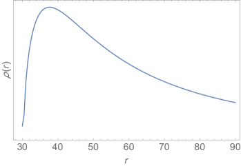
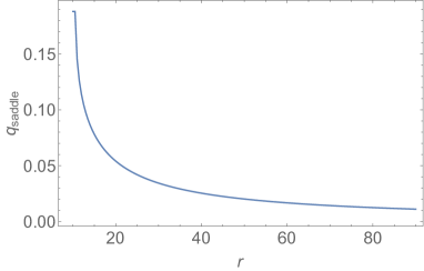
Figure 11: Left Panel : Profile of $\rho(r)$ as a function of $r$ for $N=50$. Right Panel : The value of the saddle point as a function of $r$.

In the numerical evaluation we keep track of the consistency of the saddle point by tracking the value of $q_{\texttt{saddle}}$ as a function of $r$. The large $r$ region where the saddle point approximation has less error, we find that the target profile decays. For the Amati-Ruso set-up this form factor was computed in [39] and the distribution $\rho(r)$ was shown to exactly match with that of a random walk distribution [55]. In particular one obtains that $\langle{r^{2}}\rangle\sim L$ where $L$ is the total length of the string [41]. The total string length $L$ being proportional to its mass goes like $\sqrt{N}\ell_{s}$. The intuitive picture is that the time-snap of the string is that of a random walk each of $\ell_{s}$ units, repeated $\sqrt{N}$ number of times. Therefore the extension is over the square root of this length which thus goes as $N^{1/4}\ell_{s}$. This is what one expects from the free string picture at low string couplings. At the correspondence point [11], however the entire string should lie within its Schwarzchild radius which is $\ell_{s}$. This can only be explained through a non-perturbative analysis in the string coupling as carried out in [56] using a thermal-scalar formalism. In our tree-level analysis these non-perturbative effects are ignored, therefore we expect to match onto random walk expectations.
Using the distribution $\rho(r)$ we compute numerically the mean-square spread of the string. For a normalized distribution this is defined as $\langle{r^{2}}\rangle=\int_{0}^{\infty}dr\,r^{2}\rho(r)$. Since we do not have access to the exact normalized distribution we consider a variant, a restriced-mean-square spread which we define as:

$$\langle{r^{2}}\rangle_{\texttt{R}} ={\int_{r_{\text{min}}}^{\texttt{R}}\,r^{2}\rho(r)dr\over\int_{r_{\text{min}}}^{r_{\text{max}}}\rho(r)dr}$$ (6.15)

Note, that since our saddle point evaluation limits us to start from a large enough $r_{\text{min}}>q_{\texttt{saddle}}^{-1}>0$, we need to normalize the expectation value. The value $R$, with $r_{\text{max}}>R>r_{\text{min}}$ parametrizes the string away from the centre of mass point, till where we look at the spread. For various values of $R$ we find that the restricted-mean-square spread fits to square root of $N$ scaling, consistent with the random walk picture.

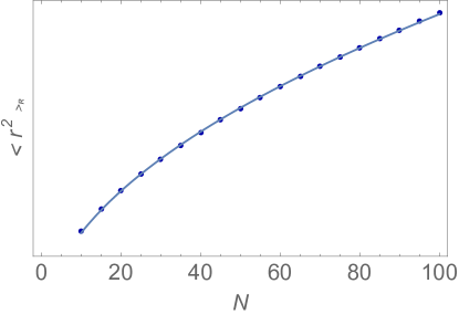
Figure 12: The above plot shows the second moment of $r$ has $\sqrt{N}$ scaling. The points are obtained from Eq.(6.15), and the line is the $\sqrt{N}$ fit.

7 Future directions

In this paper we have shown how tree-level bosonic string scattering amplitudes involving $|HES\rangle$ states contain features associated with quantum chaotic scattering, as well as quantum thermalization. Both of these features emerge statistically from the amplitudes. The statistical coarse-graining is facilitated via the large number of available microstates. The results lend support to the Susskind-Horowitz-Polchinski correspondence : the coarse-grained $|HES\rangle$ amplitudes are consistent with the thermal scales of the black hole at the correspondence point. The non-coarse-grained amplitudes themselves are statistically chaotic in the random matrix theory sense. The chaotic nature plays a key-role, as it causes huge number of cancellations when the amplitudes are coarse-grained, resulting in consistency with the eigenstate thermalization hypothesis. We hope to make this point sharper in future investigations. Additionally, we will like to point out certain suggestive directions:

• As indicated in the introduction, we will like to understand if the $HES$ S-matrix elements satisfy the non-trivial constraints as expected from a quantum gravity S-matrix which involves a black hole in the process [24]. This stems from the operator statement [57] :

  $$a^{\vphantom{\dagger}}_{\tilde{h}^{\prime}}a^{\dagger}_{h}=a^{\dagger}_{\tilde{h}}a^{\vphantom{\dagger}}_{h^{\prime}},$$

  where $a_{h}$ are annihilation operators associated with near horizon modes. The tilde on the mode indicates a shift of the Kruskal time $u$: $\tilde{h}(u)=h(u-\Delta u)$ which occurs due to quantum backreaction at the horizon from the other mode. In the L.H.S the outgoing mode has this shift, while the shift in the ingoing mode of the RHS is not seen as this mode falls inside the horizon. The change in the Kruskal time is related to the delay in the Schwarzchild time coordinate $t$, which depends on the black hole parameters. It maybe possible to match to the shift at the correspondence point, through the different kinematical orderings in the $\langle{HHTT\cdots T}\rangle$ scattering amplitude. In this respect our result in Eq.(C.5) will be useful.

• Using the techniques of [58] it should be possible to get the leading order $g_{s}$ corrections to the $|HES\rangle$ amplitudes, and understand what happens to the chaotic and the thermal features. Note, that at subleading orders in $g_{s}$, in the $AdS/CFT$ context, even the spectrum starts to show RMT statistics [59]. Going beyond the tree-level scattering will allow for:

  • Probing the Wigner time-delay [60]. This can be defined from the scattering amplitude in terms of energy derivative of the amplitude : $\Delta t=-{\cal A}^{\dagger}d{\cal A}/dE$. This time scale can be interpreted as the delay during the scattering process and is also called the dwell time. It will be interesting if this captures the Shapiro delay [61] of the black hole at the correspondence point. In the analytic plane, the scale is set by the closest distance of the resonance pole off the real-axis, however at tree-level all the poles of ${\cal A}$ are destined to appear on the real energy axis, therefore it will be necessary to go to one loop.

  • Another thing not visible in tree-level is how the long $|HES\rangle$ free string which follows the random walk picture gets squeezed into its own Schwarzchild radius, $r_{s}=\sqrt{\alpha^{\prime}}$. As discussed in [56] this is a non-perturbative effect and using effective field theory they find:

    $$r ={\sqrt{\alpha^{\prime}}\over g_{s}^{2}\sqrt{N}}.$$ (7.1)

    This relation is valid from $g_{o}<g_{s}<g_{c}$ where $g_{o}=N^{-3/8}$ and $g_{c}=N^{-1/4}$. Hence the string length $r$ interpolates from the random walk limit (at weak coupling) to the string scale at intermediate coupling. One will like to understand this calculation in the $|HES\rangle$ context from the $g_{s}$ corrections to the form factor computation. Recently the correspondence point was also discussed from this point of view in the supersymmetric case in [62].

  • In the above analysis non-perturbative techniques of [63] maybe useful. Another place where this maybe necessary will be to probe the chaotic fractal nature of the non-coarse-grained amplitude that is expected when $|HES\rangle$ states are involved. This is one of the conclusion in the absence of features from tree-level computations [31].

• The computation should be generalized to the case when the tachyon is replaced with photon. Due to extra polarization degrees of freedom available, by controlling different choices of $\zeta_{i}\cdot\zeta_{j}$ we might be able to speed-up / slow-down thermalization. Our work uncovered certain differences in the scales of chaos / thermalization when the $|HES\rangle$ polarizations were orthogonal / parallel to each other. It will be interesting to understand it completely including the role of the polarizations of the probe.

• The numerical precisions maybe pushed further in future to larger values of $N$ with smaller resolutions of scattering angles $\chi$ than considered in this work. In the context of off-diagonal ETH, Eq.(1.3), the RMT behaviour (uncorrelated random numbers) is expected to hold only for small $\omega$. It turns out that there is a critical $\omega=\Delta E_{RMT}$ which is parametrically (in system size) smaller than the corresponding time scale for thermalization [35, 64]. Going to larger levels of the $|HES\rangle$ states by pushing the numerics, will allow us to explore this scalings of $\Delta E_{RMT}$ with $N$, which in the string context is a placeholder for system size.

• It is well known that due to the KLT relations [65] closed string amplitudes can be expressed in terms of sum over open string amplitudes. Therefore using the tree-level results, one will be able to understand thermal and chaotic features of graviton scatterings within bosonic string theory. There is indication that near black hole horizons closed strings get stretched to open ones [66, 67, 68] : the $|HES\rangle$ set-up can offer a way to realize this. There are also signatures of non-adiabatic dynamics involved in horizon crossing [69], which will be interesting to realize in the $|HES\rangle$ context.

• Through the Mellin representation flat space scattering amplitudes are related to CFT correlators in Mellin space [70]. Recently similar ideas have been used to obtain via bootstrapping methods, the $AdS$ string scattering amplitudes [71], which hints towards reorganizing an arbitrary $CFT_{d}$ amplitude as string scattering amplitude in $AdS_{d+1}$. A natural question is : How the uplifted $|HES\rangle$ scattering amplitudes in $AdS$ are codified into a $CFT$ correlation function? It will be interesting to see if the answer to this question is related to the recently discussed OPE randomness hypothesis [72, 73, 74, 75] which defines random CFTs. Features of higher dimensional gravity e.g.  wormholes are known to emerge from these random CFTs [76, 77, 78].

• S-matrix elements have been computed for black holes realized in the intersection of D1-D5 systems [79]. It will be interesting to understand how chaos appears in this set-up.

• Recently [80] pointed out certain puzzles and their resolutions modulo the extremal Kerr case in the context of the black hole / string correspondence. One could explore what the $|HES\rangle$ string amplitudes can contribute towards these discussions.

Appendix A Appendix : Positivity of $\gamma$

We have:

$$q_{2}\cdot\tilde{p}_{2}=-\gamma q_{1}\cdot\tilde{p}_{2}=1.$$ (A.1)

Writing this out explicitly we obtain:

$$\gamma\left({\sqrt{N_{1}^{2}-2N_{1}(N_{2}-1)+N_{2}^{2}+2N_{2}-3}\over 2(N_{1}-1)}\cos(\beta-\theta)+{N_{1}+N_{2}-1\over 2(N_{1}-1)}\right)=1.$$ (A.2)

When, $N_{1},N_{2}\gg 1$ then using $N_{1}^{2}-2N_{1}(N_{2}-1)+N_{2}^{2}+2N_{2}-3=(N_{1}-N_{2})^{2}+2(N_{1}+N_{2})-3$ we get :

$$(N_{1}-N_{2})^{2}+2(N_{1}+N_{2})-3 \ll(N_{1}+N_{2}-1)^{2},$$

$$\text{or, }\,\,(N_{1}+N_{2}-1)\gg\sqrt{(N_{1}-N_{2})^{2}+2(N_{1}+N_{2})-3}\;\ \cos(\beta-\theta) \gg-(N_{1}+N_{2}-1).$$ (A.3)

Therefore for the first equation in Eq.(A.2) this fixes:

$$\left({\sqrt{N_{1}^{2}-2N_{1}(N_{2}-1)+N_{2}^{2}+2N_{2}-3}\over 2(N_{1}-1)}\right)\cos(\beta-\theta)+{N_{1}+N_{2}-1\over 2(N_{1}-1)} >0.$$ (A.4)

Hence we see that $\gamma$, which has the same sign as the l.h.s above is positive.

Appendix B Appendix : Total number of $HES$ states

In principle one HES might be constructed from any arbitrary number of DDF photons with arbitrary momenta. But for the simplicity of the calculation we are restricted to the case where all the constituent DDF photon momenta are parallel ($\sim nq)$ with different integer mode number $n$). The polarization of these photons can also be different. In a $d$-dimensional spacetime, each polarization vector can be linear combination of $d-2$ linearly independent null like vectors. For the process involving $2$ HES states, if we put a constraint $\lambda_{1}\cdot\lambda_{2}=$constant, then the number of choice of independent polarizations for $\lambda_{1}$ is $d-2$, and for polarization vector $\lambda_{2}$ is $d-3$, due to the constraint. the total number of microstates is given by,

$$\Omega =\Omega(N_{1})\Omega(N_{2})$$ (B.1)

$$=\underset{\{n_{r_{1}}\}}{\sum}\underset{\{n_{r_{2}}\}}{\sum}\delta(N_{1}-\sum_{r_{1}}r_{1}n_{r_{1}})\delta(N_{2}-\sum_{r_{2}}r_{2}n_{r_{2}})\prod_{r_{1}}C_{r_{1}}\prod_{r_{2}}C_{r_{2}}$$ (B.2)

$$C_{r_{1}} =\left(\begin{matrix}D-2+n_{r_{1}}-1\\ n_{r_{1}}\end{matrix}\right)=(-1)^{n_{r_{1}}}\left(\begin{matrix}2-D\\ n_{r_{1}}\end{matrix}\right)$$ (B.3)

$$C_{r_{2}} =\left(\begin{matrix}D-3+n_{r_{2}}-1\\ n_{r_{2}}\end{matrix}\right)=(-1)^{n_{r_{2}}}\left(\begin{matrix}3-D\\ n_{r_{2}}\end{matrix}\right)$$ (B.4)

$$\Omega(N_{1})\Omega(N_{2}) =\int d\beta_{1}d\beta_{2}~{}e^{\beta_{1}N_{1}+\beta_{2}N_{2}}\prod_{r_{1}}\left(e^{-\beta_{1}r_{1}}\right)^{n_{r_{1}}}\left(\begin{matrix}2-D\\ n_{r_{1}}\end{matrix}\right)\prod_{r_{2}}\left(e^{-\beta_{2}r_{2}}\right)^{n_{r_{2}}}\left(\begin{matrix}3-D\\ n_{r_{2}}\end{matrix}\right)$$ (B.5)

$$=\int d\beta_{1}d\beta_{2}~{}e^{\beta_{1}N_{1}+\beta_{2}N_{2}}\prod_{r_{1}}\left({1\over 1-e^{-\beta_{1}r_{1}}}\right)^{D-2}\prod_{r_{2}}\left({1\over 1-e^{-\beta_{2}r_{2}}}\right)^{D-3}$$

$$\sim\exp\bigg{[}{2\pi\over\sqrt{6}}\left(\sqrt{N_{1}(D-2)}+\sqrt{N_{3}(D-3)}\right)\bigg{]}.$$ (B.6)

B.1 Number of states with fixed polarizations

In our calculation we choose the DDF photon momenta of both the HES states are parallel. We also fix the polarization vectors of these photons. All the DDF photons for HES₁ have polarization $\lambda_{1}$ and similarly all the DDF photons for HES₂ have polarization $\lambda_{2}$. Here $\lambda_{1}$ and $\lambda_{2}$ both are fixed by kinamatic choice. Number of microstates in the process involving $2$ HES states (Having level $N_{1}$ and $N_{2}$ respectively) is then given by,

$$\begin{split}\Omega&=\Omega(N_{1})\Omega(N_{2})\\ &=\underset{\{n_{r_{1}}\}}{\sum}\underset{\{n_{r_{2}}\}}{\sum}\delta(N_{1}-\sum_{r_{1}}r_{1}n_{r_{1}})\delta(N_{2}-\sum_{r_{2}}r_{2}n_{r_{2}})\\ \Omega(N_{1})\Omega(N_{2})&=\underset{\{n_{r_{1}}\}}{\sum}\underset{\{n_{r_{2}}\}}{\sum}\int d\beta_{1}d\beta_{2}~{}e^{\beta_{1}N_{1}+\beta_{2}N_{2}}\prod_{r_{1}}\left(e^{-\beta_{1}r_{1}}\right)^{n_{r_{1}}}\prod_{r_{2}}\left(e^{-\beta_{2}r_{2}}\right)^{n_{r_{2}}}\\ &=\int d\beta_{1}d\beta_{2}~{}e^{\beta_{1}N_{1}+\beta_{2}N_{2}}\prod_{r_{1}}\left({1\over 1-e^{-\beta_{1}r_{1}}}\right)\prod_{r_{2}}\left({1\over 1-e^{-\beta_{2}r_{2}}}\right)\\ &=\exp\left[{2\pi\over\sqrt{6}}\left(\sqrt{N_{1}}+\sqrt{N_{2}}\right)\ \right]\end{split}$$ (B.7)

Appendix C Generalization to, $HES_{1}+T_{1}+\cdots+T_{n-k}\rightarrow HES_{2}+T_{n-k+1}+\cdots+T_{n}$ amplitude

Let’s consider the process involving $2$ HES states $H_{1}$ and $H_{2}$ and many ($n-2$) tachyons ($T_{3},T_{4}\ldots T_{n}$). The notion of ingoing and outgoing is not important here, that is encoded in the explicit form of the kinematic momenta. The amplitude can be written as,

$$\begin{split}\mathcal{A}&={1\over Vol(SL_{2})}\int\prod_{i=1}^{n}e^{\cal L}\\ \end{split}$$ (C.1)

$$e^{\cal L}=\bigg{\langle}:\prod_{r_{1}} \left(\sum_{m_{1}}^{r_{1}}{i\over(m_{1}-1)!}\zeta_{1}\cdot\partial^{m_{1}}X_{1}S^{1}_{r_{1}-m_{1}}\right)e^{ip_{1}\cdot X_{1}}::\prod_{r_{2}}\left(\sum_{m_{2}}^{r_{2}}{i\over(m_{2}-1)!}\zeta_{2}\cdot\partial^{m_{2}}X_{2}S^{3}_{r_{2}-m_{2}}\right)$$

$$e^{ip_{2}\cdot X_{2}}::e^{ip_{3}\cdot X_{3}}::e^{ip_{4}\cdot X_{4}}:\ldots:e^{ip_{n}\cdot X_{n}}:\bigg{\rangle}$$ (C.2)

For the sake of simplicity of the calculation we make kinematic choices :

$$q_{2} =\gamma q_{1},\,\,\,\zeta_{1}\cdot\zeta_{3}=\lambda_{1}\cdot\lambda_{3},$$ (C.3)

$$\zeta_{i}\cdot q_{j} =0,\,\,\,\lambda_{i}^{2}=0.$$ (C.4)

Carrying out the possible contractions yield:

$$\begin{split}\sum_{k=0}^{\{J_{1},J_{2}\}_{min}}{1\over k!}\sum_{\begin{subarray}{c}\{a(k)\}\subset\{r_{1}\}\\ \{b{(k)}\}\subset\{r_{2}\}\\ \text{ordered}\end{subarray}}&\prod_{i=1}^{k}\Bigg{[}\sum_{m_{1},m_{2}=1}^{a_{i},b_{i}}\bigg{\{}{(-1)^{m_{2}+1}(m_{1}+m_{2}-1)!\zeta_{1}.\zeta_{2}\over(m_{1}-1)!(m_{2}-1)!z_{21}^{m_{1}+m_{2}}}\bigg{\}}\\ &\times S_{a_{i}-m_{1}}\bigg{(}{a_{i}\over s_{1}}\left(\sum_{i\neq 1}{q_{1}\cdot p_{i}\over z_{i1}^{s_{1}}}\right)\bigg{)}S_{b_{i}-m_{2}}\bigg{(}{b_{i}\over s_{2}}\bigg{(}\sum_{i\neq 2}{q_{2}\cdot p_{i}\over z_{i2}^{s_{2}}}\bigg{)}\bigg{)}\Bigg{]}\\ \times&\prod_{l_{1}\in\overline{\{a(k)\}}}\Bigg{[}\sum_{n_{1}=1}^{l_{1}}\bigg{(}{\zeta_{1}\cdot p_{2}\over z_{21}^{n_{1}}}+{\zeta_{1}\cdot p_{3}\over z_{31}^{n_{1}}}\ldots+{\zeta_{1}\cdot p_{n}\over z_{n1}^{n_{1}}}\bigg{)}S_{l_{1}-n_{1}}\Bigg{]}\\ \times&\prod_{l_{2}\in\overline{\{b(k)\}}}\Bigg{[}\sum_{n_{2}=1}^{l_{2}}\bigg{(}{\zeta_{2}\cdot p_{1}\over z_{12}^{n_{2}}}+{\zeta_{2}\cdot p_{3}\over z_{32}^{n_{2}}}\ldots+{\zeta_{2}\cdot p_{n}\over z_{n2}^{n_{2}}}\bigg{)}S_{l_{2}-n_{2}}\Bigg{]}\times\prod_{i<j}z_{ij}^{p_{i}\cdot p_{j}}.\end{split}$$ (C.5)

Appendix D Appendix : Norm of the $|HES\rangle$ states

To calculate the norm of the DDF states, following [26] we use the commutation relation of DDF operators which is same as the creation operators:

$$\left[\alpha^{\mu}_{m},\alpha^{\nu}_{n}\right]=m\delta_{m,-n}\eta^{\mu,\nu}\Rightarrow\left[\lambda_{1}\cdot A_{m},\lambda_{2}\cdot A_{n}\right]=m\lambda_{1}\cdot\lambda_{2}\delta_{m,-n}.$$ (D.1)

Thus for a state with single creation operator the norm will be:

$$||\lambda\cdot A_{-m_{1}}|0\rangle|^{2}=\langle{0|\lambda^{*}\cdot A_{m_{1}}\lambda\cdot A_{-m_{1}}|0}\rangle=m_{1}|\lambda|^{2}=m_{1},$$ (D.2)

where we have used that according to our kinematic choice, $|\lambda|=1$. Thus for a generic DDF state we can write:

$$||\lambda\cdot A_{-m_{1}}\cdots\lambda\cdot A_{-m_{n}}|0\rangle|^{2} =\langle{0|\lambda^{*}\cdot A_{m_{1}}\cdots\lambda^{*}\cdot A_{m_{n}}\lambda\cdot A_{-m_{n}}\cdots\lambda\cdot A_{-m_{1}}|0}\rangle$$

$$\equiv\langle{0|A_{m_{1}}\cdots A_{m_{n}}A_{-m_{n}}\cdots A_{-m_{1}}|0}\rangle.$$ (D.3)

For a state with two creation operators, we can use commutations to obtain:

$$||\lambda\cdot A_{-m_{2}}\lambda\cdot A_{-m_{1}}|0\rangle|^{2}=\langle{0|A_{m_{1}}A_{m_{2}}A_{-m_{2}}A_{-m_{1}}|0}\rangle =m_{1}m_{2}\left(\delta_{m_{1},m_{2}}\delta_{m_{2},m_{1}}+\delta_{m_{1},m_{1}}\delta_{m_{2},m_{2}}\right)$$

$$=m_{1}^{2}\delta_{m_{1},m_{2}}+m_{1}m_{2}.$$ (D.4)

To find a general expression for DDF norms, we first look into the case for three creation operators:

In the above expression the green lines indicate the pair of indices appearing in delta functions, and the two sets of indices appear for the two sets of creation and annihilation operators. This amounts to keeping one set of indices fixed and pair all the $3!$ permutations of the other set of indices and pairing them position-wise. Each term in the expression contains all 3 indices, and collectively the expression in parentheses count the number of same indexed pairs that one can make out of $\{m_{1},m_{2},m_{3}\}$.

For example, for $\{m_{1},m_{2},m_{3}\}=\{1,2,4\}$ the only set of pair one can create is $\{(1,1),(2,2),(4,4)\}$, so only the first term contributes and the norm squared is $m_{1}m_{2}m_{3}\times 1$. But for $\{m_{1},m_{2},m_{3}\}=\{1,3,3\}$ the first and second terms in the parentheses contribute, thus the norm squared will be $m_{1}m_{2}m_{3}\times 2=m_{1}\times m_{2}^{2}\times 2!$. And for all three indices same one gets $m_{1}m_{2}m_{3}\times 3!=m_{1}^{3}\times 3!$.

Following this, we can generalize this procedure for any arbitrary number of creation operators: as one commutes an annihilation operator through the creation operators to bring it to the rightmost end, it produces a delta function for each commutation. Thus at the end one gets a sum of product of delta functions which amounts to counting the number of same indexed pairs from the annihilation and creation operators. So for a state created with $n_{m_{i}}$ number of $A_{-m_{i}}$ creation operators, the norm squared comes out to be:

$$\mathcal{N}^{2}=\bigg{|}|\underbrace{A_{-m_{k}}\cdots A_{-m_{k}}}_{n_{m_{k}}}\cdots\underbrace{A_{-m_{1}}\cdots A_{-m_{1}}}_{n_{m_{1}}}|0\rangle\bigg{|}^{2}=\prod_{i}^{k}m_{i}^{n_{m_{i}}}\cdot n_{m_{i}}!$$ (D.5)

References

- [1] L. Bombelli and E. Calzetta, Chaos around a black hole, Class. Quant. Grav. 9 (1992) 2573.
- [2] S.H. Shenker and D. Stanford, Black holes and the butterfly effect, JHEP 03 (2014) 067 [1306.0622].
- [3] S.H. Shenker and D. Stanford, Multiple Shocks, JHEP 12 (2014) 046 [1312.3296].
- [4] S. Leichenauer, Disrupting Entanglement of Black Holes, Phys. Rev. D 90 (2014) 046009 [1405.7365].
- [5] S.H. Shenker and D. Stanford, Stringy effects in scrambling, JHEP 05 (2015) 132 [1412.6087].
- [6] S.W. Hawking, Particle Creation by Black Holes, Commun. Math. Phys. 43 (1975) 199.
- [7] A. Almheiri, T. Hartman, J. Maldacena, E. Shaghoulian and A. Tajdini, The entropy of Hawking radiation, Rev. Mod. Phys. 93 (2021) 035002 [2006.06872].
- [8] A. Strominger and C. Vafa, Microscopic origin of the Bekenstein-Hawking entropy, Phys. Lett. B 379 (1996) 99 [hep-th/9601029].
- [9] C.G. Callan and J.M. Maldacena, D-brane approach to black hole quantum mechanics, Nucl. Phys. B 472 (1996) 591 [hep-th/9602043].
- [10] L. Susskind, Some speculations about black hole entropy in string theory, hep-th/9309145.
- [11] G.T. Horowitz and J. Polchinski, A Correspondence principle for black holes and strings, Phys. Rev. D 55 (1997) 6189 [hep-th/9612146].
- [12] D. Amati and J.G. Russo, Fundamental strings as black bodies, Phys. Lett. B 454 (1999) 207 [hep-th/9901092].
- [13] L. Cornalba, M.S. Costa, J. Penedones and P. Vieira, From Fundamental Strings to Small Black Holes, JHEP 12 (2006) 023 [hep-th/0607083].
- [14] R. Iengo and J.G. Russo, Semiclassical Iengo:2003ct of strings with maximum angular momentum, JHEP 03 (2003) 030 [hep-th/0301109].
- [15] B. Chen, M. Li and J.-H. She, The Fate of massive F-strings, JHEP 06 (2005) 009 [hep-th/0504040].
- [16] D. Chialva, R. Iengo and J.G. Russo, Search for the most stable massive state in superstring theory, JHEP 01 (2005) 001 [hep-th/0410152].
- [17] R. Iengo, Massless radiation from strings: Quantum spectrum average statistics and cusp-kink configurations, JHEP 05 (2006) 054 [hep-th/0602125].
- [18] T. Matsuo, Massless radiation from heavy rotating string and Kerr/string correspondence, Nucl. Phys. B 827 (2010) 217 [0909.1617].
- [19] J.L. Manes, Emission spectrum of fundamental strings: An Algebraic approach, Nucl. Phys. B 621 (2002) 37 [hep-th/0109196].
- [20] T. Kuroki and T. Matsuo, Production cross section of rotating string, Nucl. Phys. B 798 (2008) 291 [0712.4062].
- [21] A. Larkin and Y.N. Ovchinnikov, Quasi-classical method in the theory of superconductivity, Zh. Eksper. Teor. Fiz. 55 (1968) .
- [22] E. Ott and T. Tél, Chaotic scattering: An introduction, Chaos: An Interdisciplinary Journal of Nonlinear Science 3 (1993) 417.
- [23] V. Rosenhaus, Chaos in the Quantum Field Theory S-Matrix, Phys. Rev. Lett. 127 (2021) 021601 [2003.07381].
- [24] J. Polchinski, Chaos in the black hole S-matrix, 1505.08108.
- [25] E. Del Giudice, P. Di Vecchia and S. Fubini, General properties of the dual resonance model, Annals Phys. 70 (1972) 378.
- [26] D.J. Gross and V. Rosenhaus, Chaotic scattering of highly excited strings, JHEP 05 (2021) 048 [2103.15301].
- [27] M. Bianchi and M. Firrotta, DDF operators, open string coherent states and their scattering amplitudes, Nucl. Phys. B 952 (2020) 114943 [1902.07016].
- [28] M. Firrotta and V. Rosenhaus, Photon emission from an excited string, JHEP 09 (2022) 211 [2207.01641].
- [29] M. Bianchi, M. Firrotta, J. Sonnenschein and D. Weissman, Measure for Chaotic Scattering Amplitudes, Phys. Rev. Lett. 129 (2022) 261601 [2207.13112].
- [30] M. Bianchi, M. Firrotta, J. Sonnenschein and D. Weissman, Measuring chaos in string scattering processes, 2303.17233.
- [31] K. Hashimoto, Y. Matsuo and T. Yoda, Transient chaos analysis of string scattering, JHEP 11 (2022) 147 [2208.08380].
- [32] M. Srednicki, Chaos and Quantum Thermalization, cond-mat/9403051.
- [33] L. D’Alessio, Y. Kafri, A. Polkovnikov and M. Rigol, From quantum chaos and eigenstate thermalization to statistical mechanics and thermodynamics, Adv. Phys. 65 (2016) 239 [1509.06411].
- [34] C. Murthy and M. Srednicki, Bounds on chaos from the eigenstate thermalization hypothesis, Phys. Rev. Lett. 123 (2019) 230606 [1906.10808].
- [35] J. Richter, A. Dymarsky, R. Steinigeweg and J. Gemmer, Eigenstate thermalization hypothesis beyond standard indicators: Emergence of random-matrix behavior at small frequencies, Phys. Rev. E 102 (2020) 042127 [2007.15070].
- [36] M. Grinberg and J. Maldacena, Proper time to the black hole singularity from thermal one-point functions, JHEP 03 (2021) 131 [2011.01004].
- [37] S. Datta, P. Kraus and B. Michel, Typicality and thermality in 2d CFT, JHEP 07 (2019) 143 [1904.00668].
- [38] A.M. Vershik, Statistical mechanics of combinatorial partitions, and their limit shapes, Funktsional’nyi Analiz i ego Prilozheniya 30 (1996) 19.
- [39] J.L. Manes, String form-factors, JHEP 01 (2004) 033 [hep-th/0312035].
- [40] P. Salomonson and B.-S. Skagerstam, On Superdense Superstring Gases : A Heretic String Model Approach, Nucl. Phys. B 268 (1986) 349.
- [41] D. Mitchell and N. Turok, Statistical Properties of Cosmic Strings, Nucl. Phys. B 294 (1987) 1138.
- [42] V. Alba, Eigenstate thermalization hypothesis and integrability in quantum spin chains, Physical Review B 91 (2015) 155123.
- [43] P. Banerjee, A. Gaikwad, A. Kaushal and G. Mandal, Quantum quench and thermalization to GGE in arbitrary dimensions and the odd-even effect, JHEP 09 (2020) 027 [1910.02404].
- [44] G. Mandal, R. Sinha and N. Sorokhaibam, Thermalization with chemical potentials, and higher spin black holes, JHEP 08 (2015) 013 [1501.04580].
- [45] W.-Z. Guo, F.-L. Lin and J. Zhang, Note on ETH of descendant states in 2D CFT, JHEP 01 (2019) 152 [1810.01258].
- [46] E.M. Brehm and D. Das, Korteweg–de Vries characters in large central charge CFTs, Phys. Rev. D 101 (2020) 086025 [1901.10354].
- [47] B. Pozsgay, Failure of the generalized eigenstate thermalization hypothesis in integrable models with multiple particle species, Journal of Statistical Mechanics: Theory and Experiment 2014 (2014) P09026.
- [48] S. Nandy, A. Sen, A. Das and A. Dhar, Eigenstate Gibbs Ensemble in Integrable Quantum Systems, Phys. Rev. B 94 (2016) 245131 [1605.09225].
- [49] V. Burman, S. Das and C. Krishnan, To appear soon , https://youtu.be/LBFlo7msmdM?si=rzBCiMJ6sTLy728W, 2023.
- [50] J.R. David and S. Kumar, Thermal one point functions, large d and interior geometry of black holes, JHEP 03 (2023) 256 [2212.07758].
- [51] E.M. Brehm, D. Das and S. Datta, Probing thermality beyond the diagonal, Phys. Rev. D 98 (2018) 126015 [1804.07924].
- [52] A. Romero-Bermúdez, P. Sabella-Garnier and K. Schalm, A Cardy formula for off-diagonal three-point coefficients; or, how the geometry behind the horizon gets disentangled, JHEP 09 (2018) 005 [1804.08899].
- [53] Y. Hikida, Y. Kusuki and T. Takayanagi, Eigenstate thermalization hypothesis and modular invariance of two-dimensional conformal field theories, Phys. Rev. D 98 (2018) 026003 [1804.09658].
- [54] J.M. Seoane and M.A. Sanjuán, New developments in classical chaotic scattering, Reports on Progress in Physics 76 (2012) 016001.
- [55] J.L. Manes, Portrait of the string as a random walk, JHEP 03 (2005) 070 [hep-th/0412104].
- [56] G.T. Horowitz and J. Polchinski, Selfgravitating fundamental strings, Phys. Rev. D 57 (1998) 2557 [hep-th/9707170].
- [57] Y. Kiem, H.L. Verlinde and E.P. Verlinde, Black hole horizons and complementarity, Phys. Rev. D 52 (1995) 7053 [hep-th/9502074].
- [58] L. Eberhardt and S. Mizera, Evaluating one-loop string amplitudes, SciPost Phys. 15 (2023) 119 [2302.12733].
- [59] T. McLoughlin and A. Spiering, Chaotic spin chains in AdS/CFT, JHEP 09 (2022) 240 [2202.12075].
- [60] C.A. de Carvalho and H.M. Nussenzveig, Time delay, Physics Reports 364 (2002) 83.
- [61] I.I. Shapiro, Fourth test of general relativity, Physical Review Letters 13 (1964) 789.
- [62] Y. Chen, J. Maldacena and E. Witten, On the black hole/string transition, JHEP 01 (2023) 103 [2109.08563].
- [63] D.J. Gross and P.F. Mende, The high-energy behavior of string scattering amplitudes, Physics Letters B 197 (1987) 129.
- [64] J. Wang, M.H. Lamann, J. Richter, R. Steinigeweg, A. Dymarsky and J. Gemmer, Eigenstate Thermalization Hypothesis and Its Deviations from Random-Matrix Theory beyond the Thermalization Time, Phys. Rev. Lett. 128 (2022) 180601 [2110.04085].
- [65] H. Kawai, D.C. Lewellen and S.-H. Tye, A relation between tree amplitudes of closed and open strings, Nuclear Physics B 269 (1986) 1.
- [66] A. Bagchi, A. Banerjee and P. Parekh, Tensionless Path from Closed to Open Strings, Phys. Rev. Lett. 123 (2019) 111601 [1905.11732].
- [67] A. Bagchi, A. Banerjee and S. Chakrabortty, Rindler Physics on the String Worldsheet, Phys. Rev. Lett. 126 (2021) 031601 [2009.01408].
- [68] A. Bagchi, A. Banerjee, S. Chakrabortty and R. Chatterjee, A Rindler road to Carrollian worldsheets, JHEP 04 (2022) 082 [2111.01172].
- [69] E. Silverstein, Backdraft: String Creation in an Old Schwarzschild Black Hole, 1402.1486.
- [70] J. Penedones, Writing CFT correlation functions as AdS scattering amplitudes, JHEP 03 (2011) 025 [1011.1485].
- [71] R. Gopakumar, E. Perlmutter, S.S. Pufu and X. Yin, Snowmass White Paper: Bootstrapping String Theory, 2202.07163.
- [72] A. Belin and J. de Boer, Random statistics of OPE coefficients and Euclidean wormholes, Class. Quant. Grav. 38 (2021) 164001 [2006.05499].
- [73] A. Belin, J. de Boer, D.L. Jafferis, P. Nayak and J. Sonner, Approximate CFTs and Random Tensor Models, 2308.03829.
- [74] T. Anous, A. Belin, J. de Boer and D. Liska, OPE statistics from higher-point crossing, JHEP 06 (2022) 102 [2112.09143].
- [75] A. Belin, J. de Boer and D. Liska, Non-Gaussianities in the statistical distribution of heavy OPE coefficients and wormholes, JHEP 06 (2022) 116 [2110.14649].
- [76] A. Maloney and E. Witten, Averaging over Narain moduli space, JHEP 10 (2020) 187 [2006.04855].
- [77] J. Cotler and K. Jensen, AdS3 gravity and random CFT, JHEP 04 (2021) 033 [2006.08648].
- [78] J. Chandra, S. Collier, T. Hartman and A. Maloney, Semiclassical 3D gravity as an average of large-c CFTs, JHEP 12 (2022) 069 [2203.06511].
- [79] O. Lunin and S.D. Mathur, A toy black hole S-matrix in the D1-D5 CFT, JHEP 02 (2013) 083 [1211.5830].
- [80] N. Čeplak, R. Emparan, A. Puhm and M. Tomašević, The correspondence between rotating black holes and fundamental strings, JHEP 11 (2023) 226 [2307.03573].