Aspects of the Higgs phase in SU(2)U(1) lattice gauge Higgs theory
Abstract
Using a simplified lattice version of the electroweak sector of the standard model, with dynamical fermions excluded, we determine at fixed Weinberg angle the transition line between the confined phase and the Higgs phase, the latter defined as the region where the global center subgroup of the gauge group is spontaneously broken, and “separation of charge” confinement disappears. We then search, via lattice Monte Carlo simulations, for possible neutral vector bosons in the Higgs region, apart from the photon and Z. There are numerical indications of a “light Z” in the lattice data (along with the photon and the Z), but a lack of the expected scaling of the light mass particle excludes any firm conclusions about the physical spectrum.
I Introduction
The location of the Higgs phase of the Standard Model in the space of couplings depends on what one means by the Higgs phase. The earliest numerical work on the zero temperature phase diagram that we are aware of was by Shrock in *Shrock:1985un; *Shrock:1985ur; *Shrock:1986av, and a much later treatment was by Veselov and Zubkov in Zubkov:2008gi ; Zubkov:2009bk . Of course there have been a great many lattice treatments of the electroweak phase transition at finite temperature (mostly in the SU(2) gauge Higgs model, e.g. Fodor:1994sj ), as well as other topics in the electroweak theory (such as vacuum stability Kuti:2008PT ), but this article is concerned with phase structure at zero temperature. If the Higgs and confinement phases of the electroweak sector were entirely separated by a boundary of thermodynamic transition, then determination of the phase diagram at zero temperature would be fairly straightforward. However, as we know from the work of Osterwalder:1977pc ; Fradkin:1978dv ; Banks:1979fi , this is generally not the case in gauge Higgs theories with the Higgs field transforming in the fundamental representation of the gauge group. In the absence of such a boundary, it is necessary to carefully define what is meant by the “spontaneous breaking” of a gauge symmetry, which for local symmetries is actually ruled out by the Elitzur theorem Elitzur:1975im . Our view, advocated in Greensite:2020nhg , is that the Higgs phase is distinguished from the confinement and massless phases of a gauge Higgs theory by the spontaneous breaking of the global center subgroup (GCS) of the gauge group, e.g. the spontaneous breaking of the global subgroup of a local SU(N) gauge group, and this global subgroup transforms the matter fields of the theory, but does not affect the gauge fields. While the breaking of this symmetry may or may not be accompanied by a thermodynamic transition, it nonetheless is accompanied by physical effects, in particular the disappearance of metastable flux tube states in the Higgs phase, and corresponding absence of linear Regge trajectories.
In this article we first map out the transition line, using the above symmetry breaking criterion, in a simplified SU(2)U(1) lattice gauge Higgs theory, with a unimodular Higgs field (corresponding to infinite Higgs mass), and no dynamical fermions. Keeping the Weinberg angle fixed, the Wilson coupling for the SU(2) lattice field and a single parameter in the Higgs sector define a two-dimensional parameter space, and the transition line we compute lies in this plane.
A second objective is a search, via lattice Monte Carlo simulations, for new vector boson particle states within the Higgs phase whose boundary we have located. Here we note that physical particles in the electroweak theory are, in some sense, composite objects, and in any quantum theory composite objects generally have a spectrum of excitations. As ’t Hooft emphasized many years ago tHooft:1979yoe , weak isospin is actually “confined” in the electroweak sector. Certainly there is a distinction between electrons and neutrinos, but the physical particles are actually composites, with weak isospin screened by the Higgs field. The same point was made by Frohlich et al. Frohlich:1981yi and by Banks and Rabinovici Banks:1979fi . So, non-perturbatively, excited fermion states might exist. Simulations in SU(3) gauge Higgs theory strongly suggest that this may be the case Greensite:2020lmh . Unfortunately we have no reliable lattice formulation of a chiral gauge theory, so the existence of such excitations in the electroweak theory is not amenable to numerical investigation. But there is no such obstruction to a search for new states with the quantum numbers of the photon and the Z boson in a lattice formulation, providing dynamical fermions are excluded. We will see that there is evidence, in the simplified theory, for a new vector boson state, with a mass significantly lighter than the Z boson, but unfortunately that mass does not scale with lattice couplings in the way one would expect. This prevents us from drawing strong conclusions about the existence of such particles in the actual electroweak sector.
In section II we review for completeness some of the ideas presented in Greensite:2020nhg regarding the Higgs phase as a phase of broken global center symmetry. These ideas are extended to SU(2)U(1) gauge Higgs theory in section III, where the confinement to Higgs transition line, at fixed Weinberg angle, is determined. Section IV describes the results of our search for new Z boson-like excitations, and the last section contains our conclusions.
II The symmetric/Higgs phase distinction
Our view, as just mentioned, is that Higgs phase is distinguished from the confinement and Coulomb phases of a gauge Higgs theory by the spontaneous breaking of the global center subgroup (GCS) of the gauge group, and this breaking is accompanied by physical effects. In the case of a massless to Higgs transition, this is simply the appearance of a mass gap. The effect in the confinement to Higgs transition is more subtle; it is the loss of metastable color electric flux tubes which would be associated with linear Regge trajectories. This is a transition between confinement types, which were termed, in Greensite:2020nhg , “separation of charge” (S confinement and color (C) confinement, and it is not necessarily accompanied by a thermodynamic phase transition. The GCS is a subgroup of the gauge group which transforms matter fields but not gauge fields, and should not be confused with a different center symmetry which transforms gauge fields but not matter fields, with Polyakov lines as an order parameter for symmetry breaking.111In the case of SU(2) gauge Higgs theory there is a larger global SU(2) symmetry, generally known as “custodial” symmetry, which transforms the Higgs but not the gauge fields, and it was the SU(2) gauge group that was mainly considered in Greensite:2020nhg . But SU(2) is a special case, and the relevant symmetry in the general case is the global center subgroup of the gauge group.
We define a “charged” state to be a physical state, satisfying the Gauss Law constraint, which transforms covariantly under an unbroken GCS. The simplest illustration of a charged state in an infinite volume, and the motivation for this definition, is a state containing a single static fermion coupled to the quantized Maxwell field (no dynamical matter fields), presented long ago by Dirac Dirac:1955uv . In gauge the charged state is
| (1) |
where is the ground state, creates a static fermion, with
| (2) |
and Misner:1973prb
| (3) |
Let be an arbitrary U(1) gauge transformation. The ground state is obviously invariant under this transformation, while transforms covariantly. The field , however, is almost but not quite covariant under the gauge transformation. Let be the zero mode of , i.e. . Then it is easy to see that
| (4) |
and therefore, under an arbitary gauge transformation
| (5) |
In other words, a charged state in U(1) gauge theory is almost but not entirely gauge invariant. It transforms covariantly under the global center subgroup of the gauge group, consisting of transformations . If there is a dynamical matter (e.g. scalar) field in the theory which transforms in the same way as the static fermion, then one can also construct neutral states containing the static fermion, such as
| (6) |
which is invariant under the full gauge group. However, this sharp distinction between charged and neutral states breaks down if, upon inclusion of dynamical matter, the GCS is spontaneously broken, as in the Higgs phase of the abelian Higgs model. In situations of that kind, states which transform covariantly under the GCS are not necessarily orthogonal to neutral states such as above.
All of this extends directly to non-abelian gauge Higgs theories. The operator is one example of what has been called a “pseudomatter” operator Greensite:2020nhg , defined to be a functional of the gauge field which transforms like a matter field in the fundamental representation of the gauge group, except under gauge transformations belonging to the global center subgroup of the gauge group. Examples in non-abelian lattice gauge theories include gauge transformations to physical gauges, and eigenstates of the covariant lattice Laplacian on a time slice
| (7) |
where
is the lattice Laplacian, and superscripts are color indices. Note that since the lattice gauge field is unaffected by the global center subgroup of the gauge group, so are the . Using the pseudomatter operators , or any other pseudomatter operators, we can construct physical states in gauge Higgs theories such as
| (9) |
which transform covariantly under the GCS, and are charged providing that this symmetry is not spontaneously broken. A gauge Higgs theory, or any gauge theory with matter in the fundamental representation of the gauge group, is in the separation of charge (S ) confining phase if the energy expectation value of any state of this kind, above the vacuum energy, is infinite. In a finite volume one can construct finite energy states by creating separated charges
| (10) |
In the S phase the energy of such states tends to infinity as for any pseudomatter operator . In fact the statement holds for any state of this form
| (11) |
where is any functional of the gauge field only, transforming bicovariantly at the points . S confinement exists only when the GCS symmetry is unbroken. In the Higgs phase, where the GCS symmetry is broken, it can be shown that there are always some choices for which result in finite energy states as Greensite:2020nhg . The question is how to construct a gauge-invariant order parameter for the symmetry breaking.
Of course it is nonsense to regard as an order parameter. In the absence of gauge fixing this quantity is zero regardless of the couplings; in a unitary gauge it is non-zero regardless of the couplings, and in other gauges it may be zero or non-zero in various regions of coupling constant space, depending on the choice of gauge Caudy:2007sf . Following Greensite:2020nhg , we construct an order parameter starting from
| (12) |
where it is understood that on the left hand side of this equation are defined as the spatial links and scalar field on a three-dimensional time slice at , and , in lattice units, is the inverse of the lattice extension in the time direction. We then ask whether the GCS ( for SU(N)) is spontaneously broken, for a given background in the system described by the partition function . For this purpose we introduce
| (13) |
The global symmetry is spontaneously broken if is non-zero throughout the lattice. In general this quantity is not the same at each position since the background breaks translation invariance, and typically the spatial average of is negligible. It is then convenient to define the spatial average of the modulus in the spatial volume of the time slice
| (14) |
which is zero in the unbroken phase, and non-zero is the broken phase for a given background. Having derived an order parameter for global symmetry breaking at a given , we can now determine whether this symmetry is broken in the full theory by taking the expectation value
| (15) |
in the usual probability measure. If , then the global center subgroup of the gauge group is broken in every relevant configuration generated by that measure, and this is the precise meaning of the statement that global center symmetry is spontaneously broken in the Higgs phase. The order parameter is very closely analogous to the Edwards-Anderson order parameter for a spin glass Edward_Anderson , as emphasized in Greensite:2020nhg .
Here we have glossed over an important technicality. Strictly speaking, symmetries cannot be spontaneously broken in a finite volume. It is necessary to add a small term to , proportional to some constant , which breaks the global symmetry explicitly. Then the symmetry is broken if after taking first the thermodynamic and then the limit. It is possible to construct this term in a way which does not break the local gauge symmetry. For details the reader is referred to Greensite:2020nhg ; but for the numerical calculations discussed in the next section these formalities will not be necessary.
III Transition line in SU(2) U(1) gauge Higgs theory
The electroweak gauge group has a special feature: both the confined and the Higgs phases have charged states which couple to a massless particle.222It is likely, however, that at sufficiently strong couplings there is a transition within the confinement phase to a phase in which all vector particles are massive. At least, this is known to be true in other gauge theories such as the abelian Higgs model, which also contains a U(1) gauge symmetry. An example of a state of this kind is the following:
| (16) |
while a neutral state can have the form
| (17) |
and the are the Pauli matrices. Proposals of this kind (for electron and neutrino states) were made long ago in tHooft:1979yoe ; Frohlich:1981yi ; Banks:1979fi . Here are the SU(2) and U(1) lattice gauge fields respectively, and is a pseudomatter field, analogous to (2). We take the static fermion operator and the Higgs field to both transform in the fundamental representation of SU(2), but with opposite weak hypercharge . Thus transforms under a global U(1) symmetry with weak hypercharge .
In the Higgs phase, the global center symmetry is spontaneously broken. Nevertheless, in the Higgs phase, an operator which transforms as a singlet under global SU(2), and with hypercharge under global U(1), can also be regarded as transforming covariantly under a certain global U(1) transformation which is unbroken in the Higgs phase. The symmetry can be identified by going to a physical gauge defined by the gauge rotating such that upper component of vanishes, i.e.
| (18) |
and in this gauge there is a remnant local U(1) symmetry consisting of transformations
| (19) |
Under a global transformation of this type, in the Higgs phase. In the confined phase, where the global GCS is unbroken and the gauge (18) is ill-defined, we still have under a transformation .
The procedure for finding the confinement to Higgs transition in SU(2) gauge theories has been described in Greensite:2020nhg , and this procedure is unchanged for SU(2)U(1). The lattice action is
| (20) | |||||
with SU(2) gauge field and U(1) gauge field and, for simplicity, we have imposed the unimodular condition . For the lattice versions of the and photon fields in terms of in unitary gauge, cf. Veselov and Zubkov Zubkov:2008gi . The gauge and scalar fields are updated in the usual way, but each data-taking sweep actually consists of a set of sweeps in which the spacelike links are held fixed on the time slice. Let be the scalar field at site on the time slice at the -th sweep. Then we compute from the average over sweeps
| (21) |
and the order parameter from (14). Here it is important to indicate the dependence on . Then the procedure is repeated, updating links and the scalar field together, followed by another computation of from a simulation with spatial links at held fixed, and so on. Averaging the obtained by these means results in an estimate for . Since is a sum of moduli, it cannot be zero. Instead, on general statistical grounds, we expect 333One must keep in mind that at finite , would actually vanish at , since a symmetry cannot break in a finite volume. The proper order of limits is first , then . Nevertheless, for not too large, (22) is a good fit to the data, and the extrapolation should be reliable.
| (22) |
where is some constant. By computing in independent runs at a range of values, and fitting the results to (22), we obtain an estimate for at any point in the plane of lattice couplings.
III.1 Numerical results
We work throughout at fixed Weinberg angle radians. In this section we allow both and to vary and use the approach just described to compute the confinement to Higgs transition line in the plane. It is understood that in both phases there exists a massless vector boson, so not all charges are confined in either phase. But in the confined phase, at least the non-abelian charge is confined according to the S criterion. In the next section, for the computation of vector boson masses, we set , which should be close to the physical value corresponding to the usual fine structure constant.
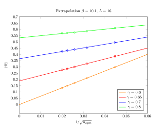
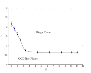
In Fig. 1 we display the extrapolation of to at on a lattice volume. For , the data extrapolates to , and the system is in the confined phase. At and above, , and the system is in the Higgs phase. The transition is for somewhere between 0.6 and 0.65. Fig. 2 shows the transition line obtained by this method, up to , on lattice volumes.444It is possible that the sudden change in slope of the transition line around is associated with a transition to a fully massive phase in the region of unbroken GCS. A similar effect was seen in SU(2) gauge theory in five dimensions, cf. Ward Ward:2021qqh .
As noted in the Introduction, the first results for the SU(2)U(1) phase diagram with a fixed modulus Higgs were obtained by Shrock Shrock:1985un ; Shrock:1985ur ; Shrock:1986av , who in fact presented phase boundary surfaces in the full three dimensional phase volume (two gauge couplings and ). In this early work the criterion for a transition was thermodynamic, i.e. non-analytic behavior of the plaquette and the Higgs action density defined below, and results were obtained by a combination of series expansions around soluble limits, and the numerical tools and methods available in the mid 1980s (the latter included estimation of transition points from hysteresis curves on very small lattices). We are calculating essentially a slice of the phase diagram in the three volume, and although it is difficult to make a precise comparison, our transition line, derived using a different criterion for the Higgs phase, appears to roughly agree with the results reported by Shrock. Our transition line is also very similar, but perhaps not exactly the same, as the line obtained in much later work by Veselov and Zubkov Zubkov:2008gi . Those authors, however, used slightly different parameters for the (renormalized) fine structure constant and the Weinberg angle, so some modest deviation is to be expected. Their criterion for a transition is also different from ours, and has to do with a drop in monopole density.
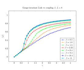
Since our criterion for a transition to the Higgs phase is non-thermodynamic, and the transition may or may not be accompanied by a thermodynamic transition, the next question is whether the confinement to Higgs transition line is also a line of thermodynamic transition. The answer appears to be similar to the SU(2) case: the symmetry breaking transition is a thermodynamic transition at large , but not at small . Define the “gauge-invariant link” as the spacetime average of the Higgs action
| (23) |
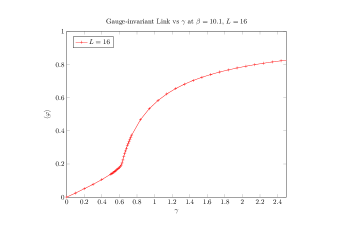
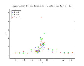
where is the lattice 4-volume. In Fig. 3 we plot the expectation value of vs. at various on a volume, and we see that while the curve is smooth at small , it seems to develop a “kink,” i.e. a discontinuity in the slope at larger . In Fig. 4 we show the same data for on a lattice volume. Precisely this type of non-analyticity has been seen before in the transition to the Higgs phase in the abelian Higgs model Matsuyama:2019lei . It is also useful to study the susceptibility,
| (24) |
at , vs. at various volumes. Note that the data point for the volume at the transition point lies well above the data points at lower volumes. All of this suggests a thermodynamic transition or, at least, a very sharp crossover around at , which is consistent with our estimate of the location of the GCS breaking transition, somewhere between and .
IV New weak vector bosons?
We search for neutral vector bosons in our simplified SU(2)U(1) gauge theory by studying correlation functions of gauge invariant operators which, operating on the vacuum, would create physical states corresponding to neutral vector bosons. Photons and physical Z bosons are states of this type, and we would like to know if there are any more in the spectrum. Define , with the lattice Laplacian operator covariant under the SU(2)U(1) group. Let be the lowest eigenstates of the Laplacian operator, with the Higgs field.
Now we use the fields to construct gauge-invariant operators which, when operating on the vacuum, will construct physical states with the quantum numbers of the physical photon and Z. Define
| (25) |
and
| (26) |
where index are spatial directions, and (which is labels the choice of pseudomatter (or Higgs) field .
Let be the transfer matrix, the vacuum energy, and
| (27) |
a modified transfer matrix. Consider two states and . Then
| (28) |
We look for states which diagonalize in the subspace of Hilbert space spanned by the such that
| (29) |
To achieve this, we compute the matrices
| (30) |
Then we solve numerically the generalized eigenvalue equation
| (31) |
or
| (32) |
There will be vectors which satisfy this equation, and then
| (33) |
are the eigenstates of in the subspace. Now we evolve these states in Euclidean time, and define
| (34) | |||||
Since, on general grounds,
| (35) |
where the are energy eigenstates (i.e. exact eigenstates of the Hamiltonian), it follows that
| (36) |
where is the energy of state above the vacuum energy (i.e. it is the energy minus ).
By construction all states are zero momentum, so for the one-particle states these are particles at rest. In that case, their masses correspond to the . If each of the were exact eigenstates of the transfer matrix in the full Hilbert space, then
| (37) |
where is one of the energy eigenvalues; in our case one of the particle masses. But that seems unlikely; we do not expect that the are exact eigenstates of the Hamiltonian. In general it is difficult to fit data to a sum of exponentials, unless the data is extraordinarily accurate. However, in our case we actually know for sure one of the masses, which is the mass of the photon, and that mass is zero. If we are fortunate, it may be enough fit each of the to the simple form
| (38) |
where is a non-zero particle mass, and is coming from an admixture of the massless photon state.
Numerically we compute
| (39) |
by lattice Monte Carlo. Note that corresponds to matrix and gives us . This provides the necessary information to determine the correlators described above.
IV.1 Numerical results
We work on a lattice at radians and . At tree-level, as in the continuum theory, there are two neutral vector bosons: a massless photon, and the Z boson. Setting the physical value GeV determines the lattice spacing, and hence in physical units
| (40) |
In the electroweak sector of the Standard Model, with a finite Higgs mass and dynamical fermions, the known value is GeV. The Z mass at tree level is
| (41) |
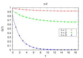
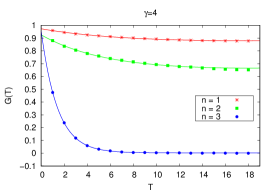
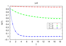
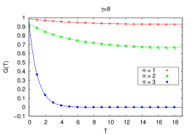
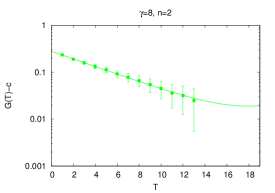
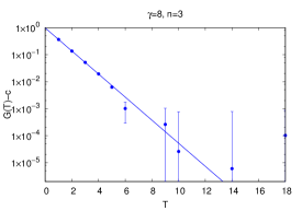
In Fig. 6 we show our data for at and , , obtained using Laplacian eigenstates and the Higgs field as described above. It is clear that the state is mostly the massless photon state, with only a small admixture of higher energy densities, given the fact that asymptotes to a flat line with . Because the falloff over a range of is so small, it is difficult for us to reliably extract the admixture of higher mass. So this mainly photon state will be excluded in the following logarithmic plots. The state also has a substantial admixture of a photon state, but for and the situation is more favorable for extracting masses, as we will see. Since our truncated Hilbert space is spanned by four states, there is also data for , but here the data is rather noisy, and not favorable for curve fitting.
At each value we have run 20 independent lattice Monte Carlo simulations consisting of 250,000 sweeps each, with 20,000 sweeps for thermalization, and data taking separated by 100 update sweeps. Each independent run supplies data for
| (42) |
with . The linear algebra required to compute is carried out by a Matlab program. To plot the data we simply average the 20 values of at each , and compute from the standard deviation. Masses can be extracted from a fit to
| (43) |
where we have allowed for periodicity in the time direction. However, cannot be interpreted as an error bar, because the chi-square of the curve fit is far too low. It is better to think of these as indicating an envelope which contains 20 separate smooth curves. An alternative procedure is to fit each of the twenty data sets to the form (43), resulting in 20 values for . This gives us an average and an error bar for the , which are the values shown in Table 1. The masses are in good agreement with the masses obtained by the first method, although we regard the second method as the appropriate procedure for obtaining error estimates on the mass values.
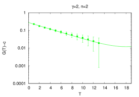
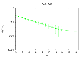
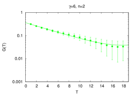
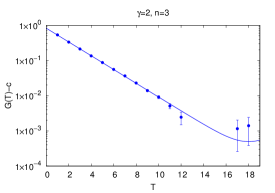
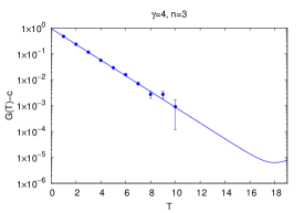
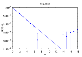
In Figs. 7 and 8 we plot the data for and respectively with the fitting constant subtracted from both the data. Having subtracted the photon component represented by the constant from the data, we display the subtracted data compared to the previous fit also with subtracted, i.e.
| (44) |
The data appears to fit a straight line on a log plot, at least for the smaller values. Deviations at larger values may be attributed to the fact that when the fitting constant is quite small, which is generally the case for , then small fluctuations in the data result in seemingly large deviations in from a straight line fit on a logarithmic plot.
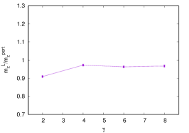
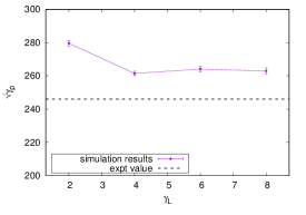
In Fig. 9 we show the ratio of the mass of the state, determined from a fit to the data, divided by the lattice tree level value in (41), and we see that the ratio, especially for , is quite close to unity, which gives us confidence in identifying the mass as the mass of the Z boson obtained in our simulations. Using these values for , we obtain a lattice spacing and a corresponding value for for each lattice coupling . These results (Fig. 10) come out close to the experimental value of GeV. All of this, together with the appearance of a zero mass (photon) state in the data, gives us some confidence that our procedure is delivering the results expected from perturbation theory.
.
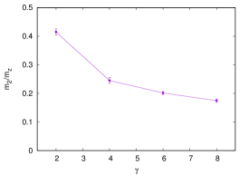
But what do we make of the intermediate mass ? The data supporting the existence of such a state, shown in Fig. 7, seems just as solid as the data for , and if we take this data seriously, it appears that the lattice regularized SU(2)U(1) theory contains an extra vector boson state, in addition to the photon and Z boson states that we have already seen, that is invisible in perturbation theory. The problem, however, is that in lattice units is almost insensitive to , and as a result the mass ratio is -dependent, as seen in Fig. 11. A first thought, since this is by construction a zero total momentum state, is that might represent two photons of opposite momenta. But for a lattice of 16 units in spatial extent, this would be a state of energy 0.79 in lattice units, which is far above . Moreover, we have checked our results on a smaller lattice of volume , with results for masses consistent (to within a few percent) with the results shown in Table 1. It seems that the data insists that is the mass of a static massive one-particle state. But this implies non-universality of the lattice action, at least so far as this intermediate mass particle is concerned. As for reasons, we can only speculate that it might be related to our unimodular condition on the Higgs field, or to the triviality of lattice theories in general.
| mass in lattice units | ||
|---|---|---|
| intermediate boson | Z boson () | |
| 2 | ||
| 4 | ||
| 6 | ||
| 8 | ||
V Conclusions
In this article we have considered an SU(2)U(1) gauge Higgs theory with a unimodular Higgs field, fixed Weinberg angle,
and no dynamical fermions. In this simplified theory we have located the transition line between the confinement and Higgs phases,
as determined from the spontaneous breaking of the global center symmetry of the gauge group. Then, in the Higgs phase, we have found at each parameter , with fixed Weinberg angle and fine structure constant, a set of three neutral vector bosons. One of these is the massless photon, and a second can be identified, because of the proximity of its mass to the tree level Z boson mass, as the Z boson. But we have also
found another massive particle state, well below the mass of the Z, which seems to be entirely non-perturbative in origin. However, the ratio of
mass of this “light Z” particle to the Z mass varies with , which indicates a non-universality in the lattice formulation. If we had obtained
results in which this ratio were fixed, then we would be able to quote a value of in physical units, and go on to wonder why such a
state has not (yet?) been seen in the collider data. However, in view of the non-universality of this ratio, such phenomenological considerations
seem premature. We speculate
that this non-universality might be associated with either our unimodular constraint on the Higgs field, or perhaps the triviality of theories. In any case, because of this non-universality, we cannot offer any predictions about the existence of a light Z in the physical spectrum of the electroweak theory. It would be interesting to repeat the calculation with a realistic Higgs potential, and we hope to report
on the results in a future publication.
Acknowledgements.
This research is supported by the U.S. Department of Energy under Grant No. DE-SC0013682.References
- (1) R. E. Shrock, Phys. Lett. B 162, 165 (1985).
- (2) R. E. Shrock, Nucl. Phys. B 267, 301 (1986).
- (3) R. E. Shrock, Phys. Lett. B 180, 269 (1986).
- (4) M. A. Zubkov and A. I. Veselov, JHEP 12, 109 (2008), arXiv:0804.0140.
- (5) M. A. Zubkov, Phys. Lett. B 684, 141 (2010), arXiv:0909.4106.
- (6) Z. Fodor, J. Hein, K. Jansen, A. Jaster, and I. Montvay, Nucl. Phys. B 439, 147 (1995), arXiv:hep-lat/9409017.
- (7) J. Kuti, PoS LATTICE 2007, 056 (2008).
- (8) K. Osterwalder and E. Seiler, Annals Phys. 110, 440 (1978).
- (9) E. H. Fradkin and S. H. Shenker, Phys.Rev. D19, 3682 (1979).
- (10) T. Banks and E. Rabinovici, Nucl. Phys. B 160, 349 (1979).
- (11) S. Elitzur, Phys.Rev. D12, 3978 (1975).
- (12) J. Greensite and K. Matsuyama, Phys. Rev. D 101, 054508 (2020), arXiv:2001.03068.
- (13) G. ’t Hooft, NATO Sci. Ser. B 59, 117 (1980).
- (14) J. Frohlich, G. Morchio, and F. Strocchi, Nucl. Phys. B190, 553 (1981).
- (15) J. Greensite, Phys. Rev. D 102, 054504 (2020), arXiv:2007.11616.
- (16) P. A. M. Dirac, Can. J. Phys. 33, 650 (1955).
- (17) C. W. Misner, K. S. Thorne, and J. A. Wheeler, Gravitation (W. H. Freeman, San Francisco, 1973).
- (18) W. Caudy and J. Greensite, Phys.Rev. D78, 025018 (2008), arXiv:0712.0999.
- (19) S. F. Edwards and P. W. Anderson, Journal of Physics F: Metal Physics 5, 965 (1975).
- (20) D. Ward, Phys. Rev. D 105, 034516 (2022), arXiv:2112.12220.
- (21) K. Matsuyama and J. Greensite, Phys. Rev. B100, 184513 (2019), arXiv:1905.09406.