A Framework for Self-Intersecting Surfaces (SOS):
Symmetric Optimisation for Stability

Abstract

In this paper, we give a stable and efficient method for fixing self-intersections and non-manifold parts in a given embedded simplicial complex. In addition, we show how symmetric properties can be used for further optimisation. We prove an initialisation criterion for computation of the outer hull of an embedded simplicial complex. To regularise the outer hull of the retriangulated surface, we present a method to remedy non-manifold edges and points. We also give a modification of the outer hull algorithm to determine chambers of complexes which gives rise to many new insights. All of these methods have applications in many areas, for example in 3D-printing, artistic realisations of 3D models or fixing errors introduced by scanning equipment applied for tomography. Implementations of the proposed algorithms are given in the computer algebra system GAP4. For verification of our methods, we use a data-set of highly self-intersecting symmetric icosahedra.

1 Introduction

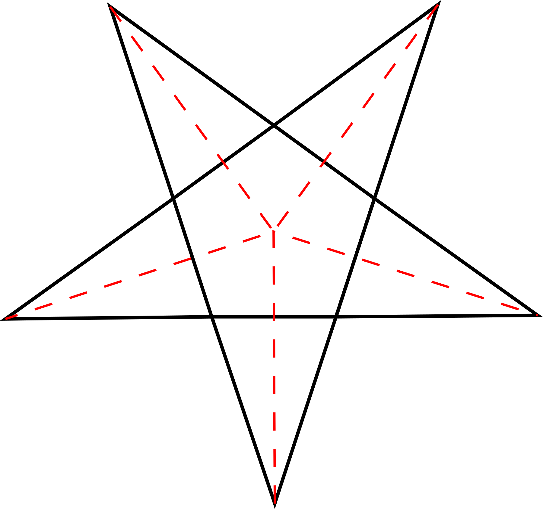
(a)

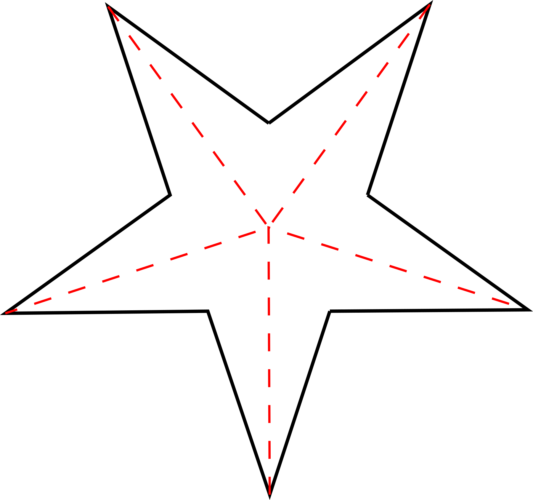
(b)

(c)

Figure 1: (a) Initial Complex with Self-Intersections; non-manifold Edges are highlighted in red-dashed Lines. (b) Outer Hull after detecting Self-Intersections and Retriangulation in Steps 1 to 3. (c) Fixture of non-manifold Parts in Step 4.

Starting with geometric data $X$ consisting of embedded triangles in $\mathbb{R}^{3}$, it is often the case that corrective actions have to be taken before handling it. For instance, $X$ could model a triangular mesh or a surface of a geometric object. Here, several techniques such as scanning methods or designing models in CAD software potentially lead to self-intersection or other artefacts.

On the other hand, one can often assume useful properties like symmetries of the given object. In this work, we focus on triangular surfaces with self-intersections and additionally enable the use of known symmetries for stability and efficiency. We model these mathematically via the terminology of embedded simplicial complexes and surfaces, which are able to describe the combinatorics of well-behaved triangular surfaces in $\mathbb{R}^{3}$. For designing purposes and other processing techniques, it is essential to compute outer hulls, see [2]. Furthermore, artefacts such as non-manifold edges and non-manifold vertices need to be addressed. In other words, focusing on the following mathematical question, we provide a framework starting with a potentially degenerate complex and ending with a well-behaved surface that satisfies the user’s need:

• How far away is an embedded simplicial complex from an embedded simplicial surface?

Given a triangulated complex $X$, we can compute its symmetry group $\text{Sym}(X)\leq\text{O}(3)$ consisting of all orthogonal transformations leaving $X$ invariant. Here, we assume that the centre of the given surface lies in the origin of the underlying coordinate system (otherwise, use translations in addition to orthogonal transformations).

This enables the use of symmetry (when applicable) for answering the above question by the following steps:

1. Compute all self-intersections of the model (using symmetry) in Sections 3 and 5.

2. Compute a retriangulation of the model (using symmetry) in Sections 5 and 4.

3. Compute the outer hull in Section 6.

4. Remedy non-manifold parts in Section 8.

These steps are shown schematically for the following example in Figure 1 above.
To guarantee a surface that is as close as possible to an initial complex, we apply robust methods throughout the framework. Furthermore, motivated by a combinatorial approach, we apply a retriangulation method that guarantees a minimal number of triangles in the resulting model.

We evaluate our methods using a dataset of icosahedra with an edge length $1$, as classified in [6] and available at [5]. Additionally, we test on surfaces with cyclic symmetry, as classified in [1]. Our algorithms are implemented in the computer algebra system GAP4 [12] which is suitable for operations with symmetry groups. In general, we can show that our symmetry algorithm leads to a speed-up in order of the number of orbits of the action of the symmetric group, see Section 5.

Example

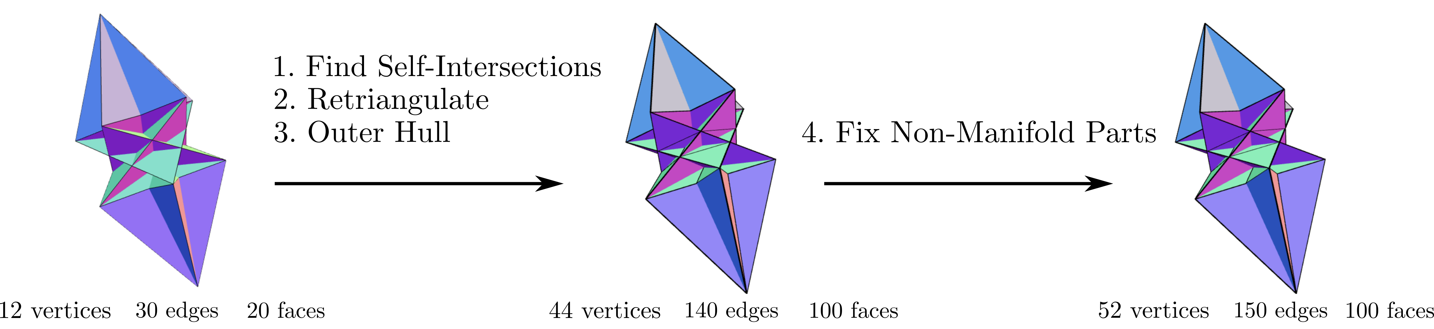
(a)

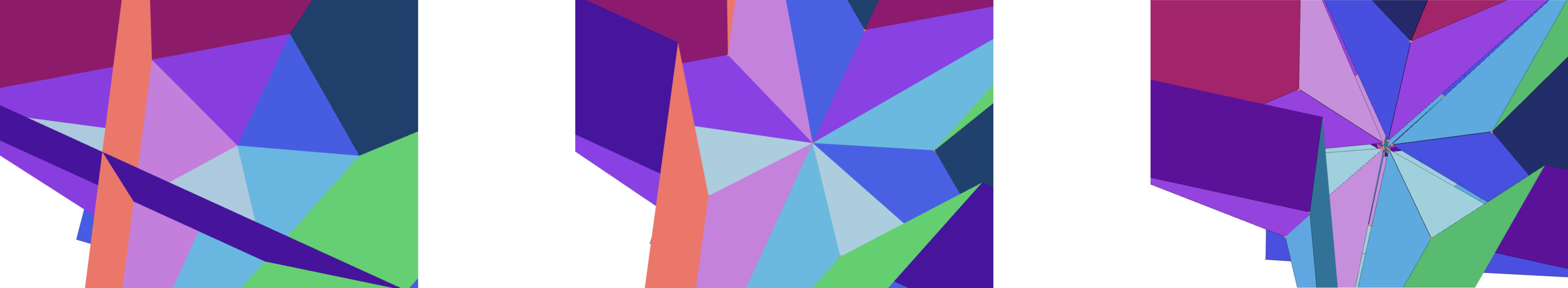
(b)

Figure 2: (a) Fixing an Icosahedron with unit Edge Lengths [6] (b) Interior in each Step

The complex $X$ shown in Figure 2(a) is combinatorally equivalent to a regular Icosahedron (a platonic solid), see Figure 3, with $12$ vertices, $30$ edges and $20$ faces and thus Euler characteristic $12-30+20=2$. Same as the standard embedding of the Icosahedron, $X$ has unit edge lengths, however, it is non-convex and there are 55 self-intersections present in the embedding of $X$. From Figure 2(a), it is clear that $X$ displays many symmetries. In fact, $\text{Sym}(X)$ has order $20$ and is isomorphic to a Dihedral group of order $20$. Locally, there are only two distinct type of faces: faces in the bottom or top and faces in the middle. Using the symmetry group, we can both simplify the determination of all self-intersections and the computation of a new triangulated complex without self-intersections $\tilde{X}$ such that $\text{Sym}(X)=\text{Sym}(\tilde{X})$ holds. Afterwards, we compute the outer hull of $\tilde{X}$ leading to a complex with $44$ vertices, $140$ edges and $100$ faces. The geometric outer hull is left invariant under our methods. However, we encounter non-manifold parts in this model that can be also seen by the Euler characteristic, which is now $4$ instead of $2$. In fact, there are in total $10$ non-manifold edges which are each connected to more than two faces. By introducing new vertices we split these edges and obtain a simplicial surface with $52$ vertices, $150$ edges and $100$ faces and Euler characteristic $2=52-150+100.$

Related Work

Self-intersections and non-manifold parts of models are very active fields of research. This is because of the obstructions they cause in many fields, such as meshing, scanning of 3D-models, and 3D-printing [2, 10, 23, 27].
In [2], the author presents an algorithm to compute the outer hull, which we also apply and modify to compute all chambers of the given complex. Furthermore, the author provides an initialisation criterion for which we add a mathematical proof. In [27], the authors describe a robust method to rectify self-intersections of a complex and use a subdivision based on Delaunay triangulation with certain constraints to retriangulate the initial complex.
Focusing on self-intersections in triangulated complexes, there are several approaches for finding all self-intersections or testing if two given triangles intersect, for instance [18, 17]. Also, see [21] for a recent review on algorithms for the detection of self-intersections. Repairing and retriangulation methods can be found in [3] for a direct approach, which is also suitable for the computation of outer hulls, [16] for a method using immersion techniques, [26] for a method employing edge swap techniques, and [8] for a method using a combination of an adaptive octree with nested binary space partitions (BSP), to name a few. Works on remedying non-manifold parts can be found in [20, 23, 11]. Another similar direction is the treatment of meshes and their repair, as done in [10]. As an input to our model, we use the symmetries of a given complex, which leads to simplification and speed up the algorithms. Of course, this is an idea that can be applied to different settings, such as in model segmentation in [14]. In conjunction with the ideas we present, one can consider detection of symmetries in surfaces, as in [15], [7].

2 Preliminaries

In this section, we introduce the main terminology used in this work. We start by giving a definition of an adapted version of simplicial complexes corresponding to a triangular surface, motivated by the combinatorial theory of simplicial surfaces, see [4, 19].

Definition 2.1 (Simplicial Complex).

Let $V$ be a finite set. A closed simplicial complex $X$ with vertices $V$ is a subset of $\mathcal{P}_{3}(V)=\{A\subset V:|A|\leq 3\}$ such that the following conditions hold.

1. For all $v\in V$, $\{v\}\in X$. Additionally, $\emptyset\not\in X$.

2. For each $\emptyset\neq x\subset t\in X$ it follows that $x\in X$.

3. For each $t\in X$, $|t|<3$, we can find $|t^{\prime}|>|t|$ with $t\subset t^{\prime}$ and $t\in X$.

4. For each $f\in X$ with $\lvert f\rvert=3$ and each $v_{1},v_{2}\in f$, we can find $f^{\prime}\neq f$ such that $v_{1},v_{2}\in f^{\prime}$.

We call the three-element sets in $X$ the faces or triangles $f_{i}$, the two-element sets in $X$ the edges $e_{i}$ and the one-element sets in $X$ the vertices $v_{i}$. Write $X_{2}$ for the faces, $X_{1}$ for the edges and $X_{0}$ for the vertices. We also call $v_{i}$ incident to the edge $e_{j}$ or $e_{j}$ incident to $f_{k}$ if $v_{i}\in e_{j}$ or $e_{j}\in f_{k}$, respectively. Since there will be no other complexes other than simplicial ones, we may omit the word simplicial.

The conditions in the definition above all correlate to natural assumptions for a surface made up of triangles. For example, since we consider $\mathcal{P}_{3}(V)$, the faces are triangles. The conditions $(i)-(iv)$ are interpreted as follows:
$(i)$ gives that the vertex set on which our surface is build is actually part of it.
$(ii)$ implies that if we take a face or edge, its parts are also included in the description of the surface.
$(iii)$ enforces that each vertex is part of an edge and each edge is part of a face.
$(iv)$ forces the surface to be closed, so every edge has to be incident to at least two faces.
In total, we observe that a simplicial complex $X$ is uniquely determined by its faces.

We also make the following definition of faces associated to a given vertex.

Definition 2.2.

Let $X$ be a simplicial complex and take a vertex $v$ of $X$. Define the faces incident to $v$ to be the set $X_{2}(v)\coloneqq\{f\in X:v\in f\text{ and }|f|=3\}$.

A more regular object is a simplicial surface, which corresponds to a natural incidence relation on a triangular surface.

Definition 2.3 (Simplicial surface).

A closed simplicial surface $S$ is a closed simplicial complex that additionally fulfils the following.

1. For all faces $f_{1},f_{2},f_{3}\in S$ with $|f_{1}\cap f_{2}\cap f_{3}|=2$ it holds that $|\{f_{1},f_{2},f_{3}\}|=2$.

2. For all vertices $v\in V$ we can order all the faces incident to $v$, i.e. the set $S_{2}(v)$, in a cycle $(f_{1},\dots,f_{n})$ such that $f_{i}$ and $f_{i+1}$ (and additionally $f_{1}$ and $f_{n}$) share a common edge.

The above conditions turn out to be crucial for identifying non-manifold parts of embedded simplicial complexes considered in the following sections. For example, the first condition directly corresponds to no non-manifold edges being present in the complex. The second condition is called the umbrella condition. The vertices that do not fulfil it are called non-manifold vertices. More general defintions of simplicial surfaces, also allowing distinct faces with the same set of incident vertices can be found in [19, 4, 1].

Definition 2.4 (Embedding).

An embedding of a simplicial complex $X$ with vertices $V$ is an injective map

$$\phi:V\to\mathbb{R}^{3}.$$

We write $(X,\phi)$ for a complex $X$ with embedding $\phi$. Thus we also write $\phi(e)=\{\phi(v_{1}),\phi(v_{2})\}$ for edges $e\in X$ and similarly for faces $f\in X$. If a given complex $X$ is embedded into $\mathbb{R}^{3}$, we omit the map $\phi$ whenever it is clear from the context. Moreover, we often identify the vertices, edges and faces with their resp. images under $\phi$.

In the definition above, the map $\phi$ is chosen to be injective to avoid degenerate edges and faces. Additionally, we can obtain the initial underlying complex $X$ from its embedding $\phi(X)$.

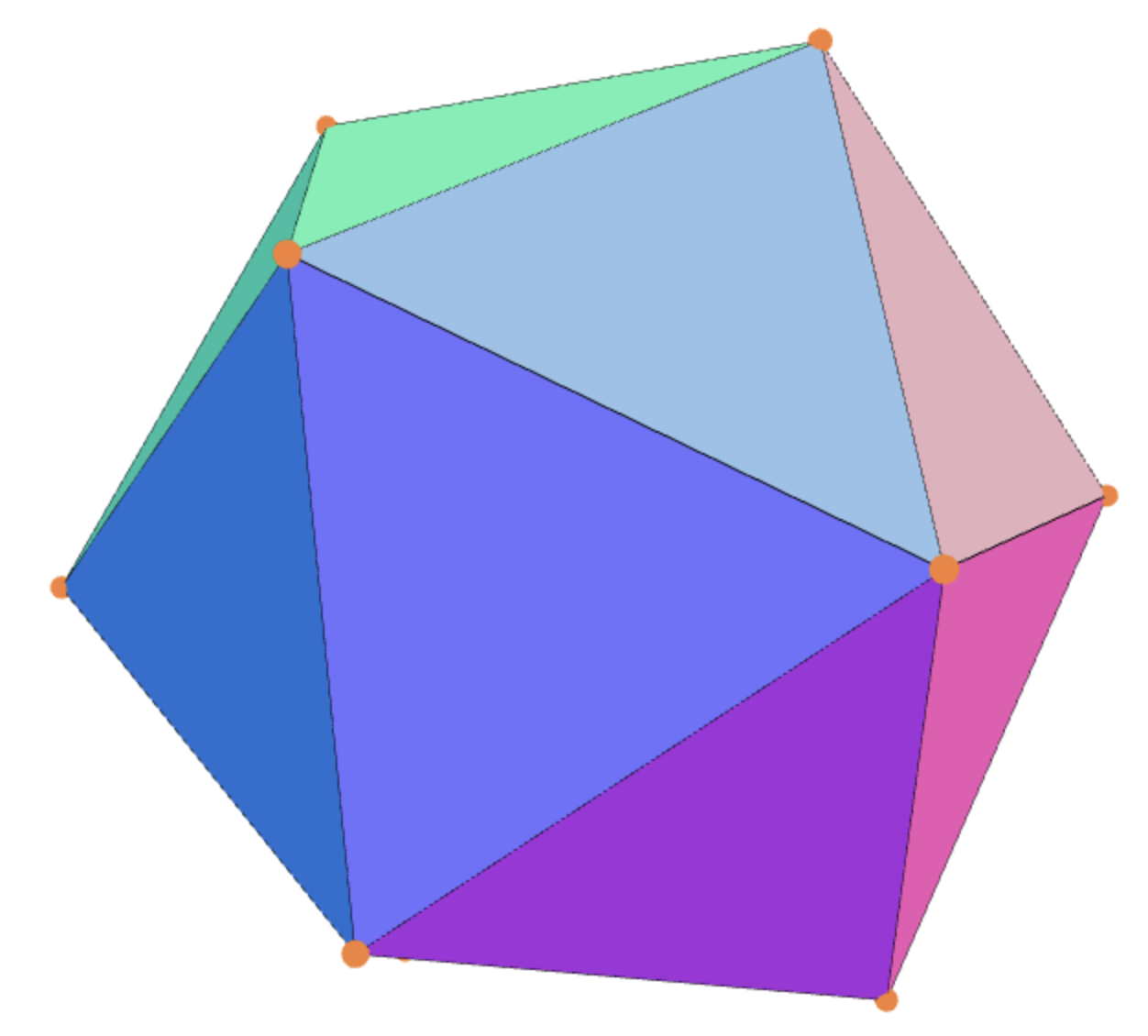
(a)

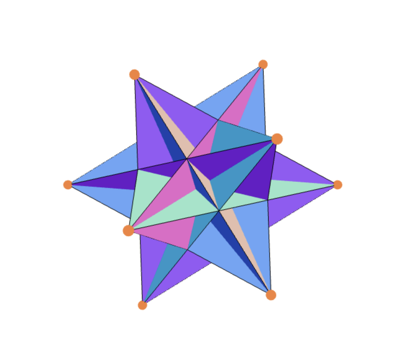
(b)

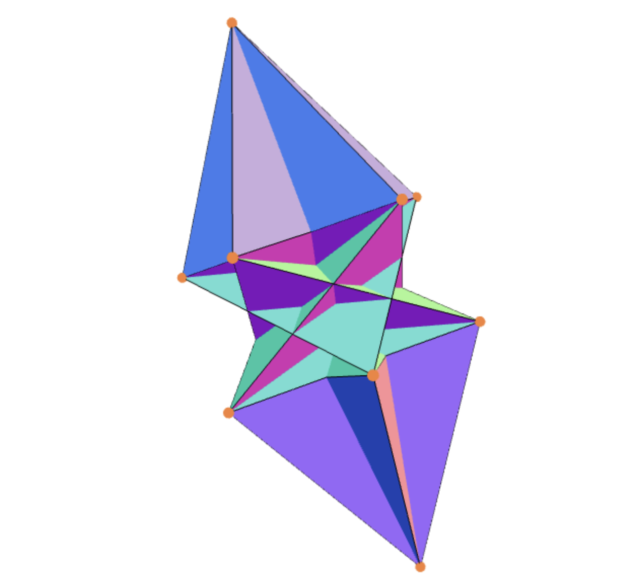
(c)

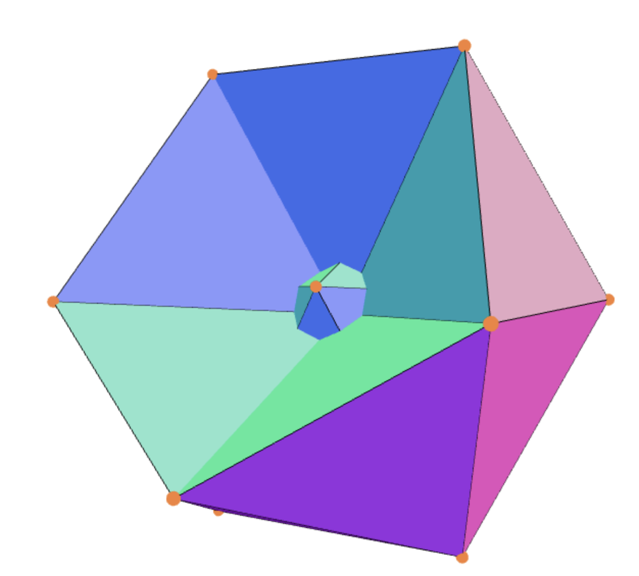
(d)

Figure 3: One simplicial Surface (Icosahedron) with distinct Embeddings of unit Edge Length [6]: (a) Platonic Solid (b) The Great Icosahedron (c) Icosahedron_3_1 (d) Icosahedron_3_2 (Notation given in [5])

In Figure 3, we see several distinct embeddings of the same underlying simplicial surface.

Remark 2.5.

The map $\phi$ above can be represented as a list with $|V|$ entries in $\mathbb{R}^{3}$ or alternatively as a matrix in $\mathbb{R}^{|V|\times 3}$. Thus, one can switch from the algebraic structure of an embedded simplicial complex to one used in application, such as a coordinate representation or an STL file. Here, it suffices to store the embedding data suitably, for example via a list of lists.

We can define the orientation of a simplicial surface in a combinatorial way below.

Definition 2.6 (Orientation).

An orientation of a simplicial surface $S$ is given by a cyclic ordering of the three vertices of each face, such that for any given edge $\{v_{1},v_{2}\}=e=f_{1}\cap f_{2}$ of two incident faces, we have that either the ordering of $f_{1}$ is $(v,v_{1},v_{2})$ and the one of $f_{2}$ is $(v^{\prime},v_{2},v_{1})$ or the other way around with ordering of $f_{1}$ by $(v,v_{1},v_{2})$ and $f_{2}$ by $(v^{\prime},v_{1},v_{2})$.

This can be used to give a normal vector for each face pointing to the outside.

Remark 2.7.

If an embedded surface is orientable, we can define the outer normals for each face as follows: Let $f=\{v_{1},v_{2},v_{3}\}$ such that the vertices are ordered as $(v_{1},v_{2},v_{3})$, then the outer normal is given by the right-hand rule

$$(v_{2}-v_{1})\times(v_{3}-v_{1}).$$

Alternatively to the combinatorial approach of defining an orientation and related outer normals for an embedding, we give the geometric definition of chambers and the outer hull for an embedded complex as follows.

Definition 2.8 (Chambers and outer hull).

The chambers of the embedded complex $X$ are defined as the connected components of $\mathbb{R}^{3}\setminus\bigcup_{f\in X_{2}}\text{conv}(f)$. The outer hull $X_{\text{out}}$ is the boundary of the unique chamber $O$ with infinite volume.

Note that since we require $S$ to be closed and the embedding to be injective, the set $W$ from Definition 2.8 exists and is non-empty. Therefore, it is reasonable to consider applications such as 3D printing of the surface, as the object possesses a well-defined inner volume.

With this definition in mind, we can also define when a point is contained inside the embedded complex.

Definition 2.9.

Let $X$ be an embedded simplicial complex. We say that a point $p\in\mathbb{R}^{3}$ is contained in $X$ if it is either contained in one of the finite volume chambers of $X$ or in one of the faces.

With this, we can give a more intuitive and equivalent definition of the outer hull as follows.

Remark 2.10.

The outer hull of an embedded complex $X$ can be also viewed as the maximal subset $X_{\text{out}}\subset X$ such that there exists a non-intersecting path from any far away point not contained in $X$ to each face of $X_{\text{out}}$.

Another central term is intersection points,i.e. points where triangles of the complex meet, but which are not vertices or on common edges.

Definition 2.11 (Intersection points).

Let $(X,\phi)$ be an embedded simplicial complex. We say that the embedding (or just $X$) has an intersection point $p\in\mathbb{R}^{3}$ if there exist faces $f_{1},f_{2}$ such that $p\in\mathrm{conv}(\phi(f_{1}))\cap\mathrm{conv}(\phi(f_{2}))$ and $p\not=\phi(v)$ for all vertices $v\in f_{1}\cap f_{2}$. Write $I(X,\phi)$ for the collection of all intersection points and $I(X,\phi,f):=I(X,\phi)\cap\mathrm{conv}(\phi(f))$ for the collection of all intersection points of a fixed face $f$. If $I(X,\phi)$ is empty, we call the embedded surface intersection-free, else we say that it has self-intersections, as in Figure 4.

Rectifying intersections points is important to be able to infer about the outside and inside of our embedded surface, as is described in Remark 2.12.

(a) Intersection of two faces

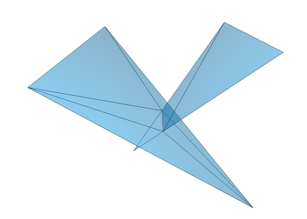
(b) Retriangulation of the two faces

Figure 4: Intersection of Triangles inside a Complex $X$

Together with the embedding, the normal vectors are sufficient to create a 3D model of the simplicial complex, as seen in [25]. But if an embedding has a self-intersection, the following needs to be considered.

Remark 2.12.

Note that the outer hull of an embedded complex is well-defined even in the case that the embedding has self-intersections. However, then our description of the complex is not sufficient to compute it, as can be seen in Figure 4. This is because faces can lie in multiple chambers at once, and thus we can not use normals to infer about the outer hull. For example, if we can assumed the faces to be on the outer hull and tried to define the outer normal of the left triangle to be pointing towards the upper right. But then both the area above and below the right triangle would have to be outside of $X$, which gives a contradiction.

3 Detecting Self-Intersections

In order to retriangulate a complex with self-intersections, we first need to detect its self-intersection points. Since our main focus lies on giving a robust retriangulation, we employ a well-known and robust way to check if two triangles intersect. Since our methods are modular, one could also use state of the art intersection detection algorithms such as PANG2 (see [17]) instead.

Consider a simplicial complex $X$ with embedding $\phi$, two faces $f_{l}=\{v_{1}^{l},v_{2}^{l},v_{3}^{l}\},\ l=1,2$ in $X$ and their respective vertices. For simplicity, we identify the vertices of $X$ with their images under the embedding $\phi$. In the following, we use the standard Euclidean dot product

$$\langle\cdot,\cdot\rangle:\mathbb{R}^{3}\times\mathbb{R}^{3}\to\mathbb{R},(x,y)\mapsto\langle x,y\rangle=x^{tr}\cdot y.$$

We determine the intersections by examining the edges between vertices of $f_{1}$ and use the normal equation of the plane $P(f_{2})$ spanned by $v^{2}_{1},v^{2}_{2}$ and $v^{2}_{3}$ to compute when these intersect the plane in a point $p$. Afterwards, we have to check if $p$ lies inside the triangle $f_{2}$. For an edge $\{v_{i}^{1},v_{j}^{1}\}=e\subset f_{1}$, we have to distinguish between the following two cases:

1. $e$ is not parallel to $f_{2}$.

2. $e$ is parallel to $f_{2}$.

Case $(i)$ holds if and only if $\langle v^{1}_{j}-v^{1}_{i},n_{f_{2}}\rangle\neq 0$, where $n_{f_{2}}$ is the unit normal vector of the face $f_{2}$. So assume first that this holds, and treat $(ii)$ later on.

If $n_{f_{2}}$ is a normal vector of the plane $P(f_{2})$, containment of a point $p$ is in the plane $P(f_{2})$ can be described as follows:

$$p\in P(f_{2})\iff\langle p-v^{2}_{1},n_{f_{2}}\rangle=0.$$ (1)

Thus, for points of the line connecting $v_{i}^{1}$ and $v_{j}^{1}$ given by $l_{ij}(\alpha):=\alpha v_{j}^{1}+(1-\alpha)v_{i}^{1}$, we get

$$l_{ij}(\alpha)\in P(f_{2})\iff\alpha=\dfrac{\langle v^{2}_{1}-v^{1}_{i},n_{f_{2}}\rangle}{\langle v^{1}_{j}-v^{1}_{i},n_{f_{2}}\rangle}.$$ (2)

To then check if the intersection point $p$ is contained in the edge of $f^{1}$, $\alpha\in[-\varepsilon,1+\varepsilon]$ for a small $\varepsilon>0$ needs to hold (where the $\varepsilon$ accounts for numerical errors).

If we find a point $p$ that lies in the plane $P(f_{2})$, we need to check if it is actually contained inside the triangle $f_{2}$. For this, we use the following geometric approach: If $p$ sits inside the face $f_{2}$, its scalar product for all $i\in\{1,2,3\}$ with the normal $\tilde{n}_{i}$ of the plane spanned by $n_{f_{2}}$ and $v_{i}^{2}-v_{j}^{2}$ (for an fixed $j\neq i$) has to be non-negative if $\tilde{n}_{i}$ points towards the inside of the face.
With this information, we can ensure the correct orientation of the normal vectors and then simply check if $\langle\tilde{n}_{1},v_{0}\rangle\geq-\varepsilon$ for $i\in\{1,2,3\}$.

For the second case that the edge is contained in the plane $P(f_{2})$, we need to distinguish between the following cases:

1. The edge is contained in a parallel plane different from the triangle

2. The edge is contained in the same plane as the triangle and

   1. Does not intersects inside the triangle,

   2. Intersects the triangle,

   3. Lies inside the triangle.

For a treatment of these cases, we refer to [22].

By using the methods described above, we compute all intersection points $I_{2}$ of edges of $f_{1}$ with $f_{2}$. We also need the reverse: the intersection points $I_{2}$ of edges of $f_{2}$ with $f_{1}$, as seen in Figure 5.

Figure 5: Edges of both Faces need to be considered

After accounting for numerical duplicates, we examine $I_{1}\cup I_{2}$, as its cardinality $c:=|I_{1}\cup I_{2}|$ determines if the faces intersect non-trivially: Only if, $c=2$, the faces intersect, as can be seen in Figure 6. The intersection is then parameterised by $v_{1},v_{2}$ with $I_{1}\cup I_{2}=\{v_{1},v_{2}\}$.

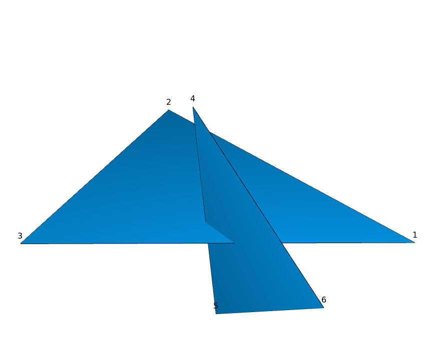
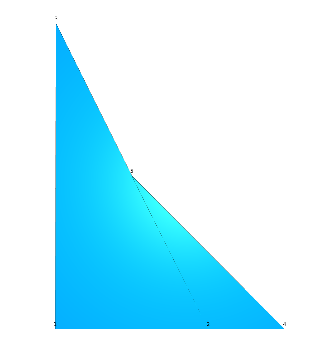
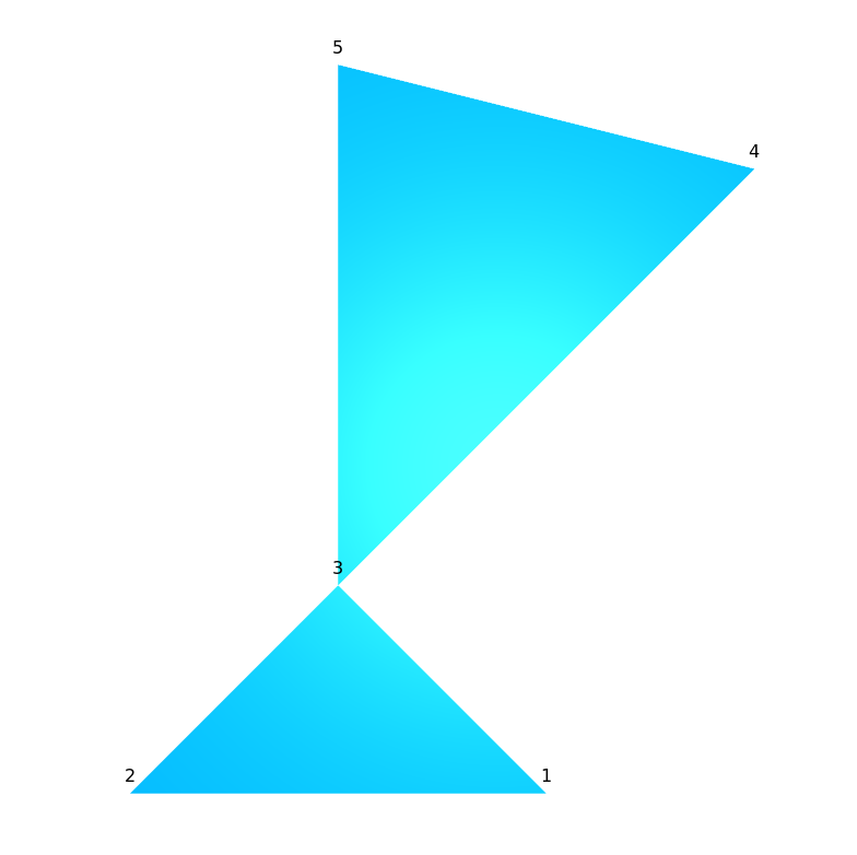
Figure 6: Intersection of Triangles (left, middle) vs no Intersection (right)

4 Retriangulation

In this section, we introduce an algorithm that yields a retriangulation of an embedded complex with self-intersections. In the Section 3 we give a method for computing all self-intersections of face pairs and showed that it suffices to retriangulate one face after another.

Now, given a face $f\in X$ with intersections given by the set $I(X,\phi,f)$, where $(X,\phi)$ denotes the underlying embedded complex. Below, we give a data structure that contains all self-intersections of $f$ with other faces as a list $l$ with two entries:

1. In the first entry, $l$ contains all embedded data of vertices $V$ of $f$, and all vertices given by the intersections with other faces.

2. In the second entry of $l$ the edges that connect two vertices are given as pairs of distinct vertices.

The starting step is to search for edge intersections and containment of vertices in edges. Note that here, for a set $Y$, $Y^{(k)}:=\{g:\{1,\dots,k\}\rightarrow Y\text{ injective}\}$ for $k\in\mathbb{N}$ is the set of $k-$tuples with pairwise distinct entries.

input: Triangle together with intersection points $l[1]\subset\mathbb{R}^{3},l[2]\subset V^{(2)}$

output: $l$ has no-self intersections

begin

       $l\leftarrow CleanData(l)$

       $edges\leftarrow l[2]$

       $vertices\leftarrow l[1]$

       for $v\in vertices$ do

             for $e\in edges$  do

                   if $v$ is contained in $e$ then

                         $edges\leftarrow edges\setminus e\cup\{\{v,e[1]\},\{v,e[2]\}\}$

                         /* edge $e$ is split via vertex $v$ */

                        

                   end if

                  

             end for

            

       end for

      $l\leftarrow CleanData(l)$

       $edgepairs\leftarrow edges^{(2)}$

       for $edgepair\in edgepairs$ do

             if $edgepair[1]$ intersects $edgepair[2]$ in $v\notin l[1]$ then

                   $edges\leftarrow edges\setminus\{edgepair[1],edgepair[2]\}$

                   $edges\leftarrow edges\cup\{\{v,edgepair[2][1]\},\{v,edgepair[2][2]\}$

                   $edges\leftarrow edges\cup\{\{v,edgepair[1][1]\},\{v,edgepair[1][2]\}\}$

                   /* edges $edgepair[1],edgepair[2]$ intersect in a vertex $v$ */

                  

             end if

            

       end for

      $l\leftarrow CleanData(l)$

       return l

      

end

Algorithm 1 Fixing intersection in a triangle

Next, we retriangulate the cleaned list $l$ given as an output of Algorithm 1. For this, we introduce the following termination criterion indicating when we inserted enough edges to receive a triangulated disc.

Lemma 4.1.

The Euler characteristic of a disc is given by

$$V+(E+E^{\prime})-\frac{E+(E+E^{\prime})}{3}=1,$$ (3)

where $V$ is the number of vertices and $E$ resp. $E^{\prime}$ the number of inner resp. boundary edges.

Proof.

Gluing together two identical discs at their boundary leads to a sphere with $2V+V^{\prime}$ vertices and $2E+E^{\prime}$ edges. The number of faces in a closed simplicial sphere equals $2E/3$ and its Euler Characteristic is equal to $2$. Hence, we have

$$2V+V^{\prime}-(2E+E^{\prime})+\frac{2(2E+E^{\prime}))}{3}=2.$$

Using the face that the number of boundary vertices $V^{\prime}$ equals the number of boundary edges $E^{\prime}$, we arrive at the desired statement above. ∎

Now, to triangulate $l$, it suffices to add non-self intersecting edges until condition 3 is fulfilled. For this, we first compute the number of boundary vertices $V^{\prime}$ of $l$, which equals the number of boundary edges $E^{\prime}$ and thus use that $E+E^{\prime}=\lvert l[2]\rvert,V=\lvert l[1]\rvert$. Since we only need to add inner edges $E$, we can compute the number of total internal edges by

$$E=3V-2E^{\prime}-3.$$

Therefore we only need to add $3\cdot\lvert l[1]\rvert-2E^{\prime}-3-\lvert l[2]\rvert$ edges.

input: $l$ has no self-intersections

output: $l$ is triangulated

begin

       $possibleedges\leftarrow V^{(2)}$

       $possibleedges\leftarrow SortByLength(possibleedges)$

       while $V-(E+E^{\prime})+\frac{E+(E+E^{\prime})}{3}\neq 1$ do

             $e_{1}\leftarrow\text{possibleedges}[1]$

             $possibleedges\leftarrow\text{possibleedges}\setminus e_{1}$

             $foundnewedge\leftarrow\text{true}$

             for $e_{2}\in l[2]$ do

                   if $e_{1}$ intersects $e_{2}$ then

                         $ok\leftarrow\text{false}$

                         /* edge $e$ is split via vertex $v$ */

                         break

                        

                   end if

                  

             end for

            

       end while

      $l\leftarrow\text{CleanData}(l)$

       $edgepairs\leftarrow\text{edges}^{(2)}$

       for $edgepair\in\text{edgepairs}$ do

             if $\text{edgepair}[1]$ intersects $\text{edgepair}[2]$ in $v\notin l[1]$ then

                   $\text{edges}\leftarrow\text{edges}\setminus\{\text{edgepair}[1],\text{edgepair}[2]\}$

                   $\text{edges}\leftarrow\text{edges}\cup\{\{v,\text{edgepair}[2][1]\},\{v,\text{edgepair}[2][2]\}\}$

                   $\text{edges}\leftarrow\text{edges}\cup\{\{v,\text{edgepair}[1][1]\},\{v,\text{edgepair}[1][2]\}\}$

                   /* edges $\text{edgepair}[1]$, $\text{edgepair}[2]$ intersect in a vertex $v$ */

                  

             end if

            

       end for

      

end

Algorithm 2 Triangulation of data $l$

Algorithm 2 terminates for arbitrary inputs.

5 Symmetry

Symmetry of a given embedded complex $X$ can be used in two ways to simplify computations for finding and fixing self-intersection:

1. Finding self-intersections: consider only face pairs up to symmetry,

2. Retriangulation: only fix self-intersections and retriangulate one face in each orbit of the symmetry group acting on the faces.

The orthogonal group $\text{O}(3)$ defined by rotation and reflection matrices acting on the real-space $\mathbb{R}^{3}$ consists of $3\times 3$-matrices $A$ with $A^{tr}\cdot A=\mathbb{I}$, i.e. matrices $A$ with inverse given by their transposed matrix. The standard scalar product of two vectors $x,y\in\mathbb{R}^{3}$ is thus invariant under multiplication of an orthogonal matrix $A$ since we have

$$\langle Ax,Ay\rangle=\left(Ax\right)^{tr}\left(Ay\right)=x^{tr}A^{tr}Ay=x^{tr}y=\langle x,y\rangle.$$

Given an embedded complex $X$, we can define its symmetry group $G\coloneqq\text{Sym}(X)\leq\text{O}(3)$ by all orthogonal transformations leaving $X$ invariant, i.e.

$$\text{Sym}(X)\coloneqq\{\pi\in\text{O}(3)\mid\pi(X)=X\},$$

where the action of an element $\pi\in\text{O}(3)$ on a complex $X$ is defined by applying $\pi$ to the 3D-coordinates of each vertex.

The symmetry group $G$ induces subgroups of the automorphism group $\text{Aut}(X)$ of the underlying simplicial complex $X$, i.e. subgroups of the symmetry group on the vertices, edges and faces. These permutation groups can be used when computing face and face-pair orbits. Switching to a discrete permutation group allows both faster and precise computations without the use of numerical methods.

The group $G$ acts on the set of faces $X_{2}$ of the given complex. Before remedying the self-intersections, as in Section 4, we can determine a transversal of the orbits of $G$ on the set of faces, that is a minimal set of faces $\{f_{1},\dots,f_{n}\}$ with

$$\bigcup_{i=1}^{n}G(f_{i})=X_{2}.$$

Thus each face of the complex can be obtained by applying certain symmetries onto a face in the much smaller set $\{f_{1},\dots,f_{n}\}$.

When computing self-intersection, we have to consider face pairs $(f_{1},f_{2})$. We can extend the action of $G$ on the faces $X_{2}$ to the pairs of distinct faces, denoted by $X_{2}^{(2)}$. Hence, it suffices to consider the orbits defined by this group action instead of considering all face pairs

$$G\times X_{2}^{2}\to X_{2}^{2},\big{(}g,(f_{1},f_{2})\big{)}\mapsto(g(f_{1}),g(f_{2})).$$

Here, the face $f_{1}$ resp. $f_{2}$ is transformed onto $g(f_{1})=f_{1}^{\prime}$ resp.  $g(f_{2})=f_{2}^{\prime}$ by applying an element $g$ in the symmetry group $G$. Now we can observe that the faces $f_{1},f_{2}$ intersect if and only if the faces $f_{1}^{\prime},f_{2}^{\prime}$ intersect. Let $I_{f_{1},f_{2}}=f_{1}\cap f_{2}$ denote the intersection of two faces. With the notation above it follows that

$$g(I_{f_{1},f_{2}})=I_{f_{1}^{\prime},f_{2}^{\prime}}.$$

This means that it suffices to only consider one element of the orbit

$$G((f_{1},f_{2}))\coloneqq\{(g(f_{1}),g(f_{2}))\mid g\in G\}$$

to determine all intersections of face pairs in this set.

Combining both observations of the group actions of $\text{Sym}(X)$ on the faces $X_{2}$ and face pairs $X_{2}^{(2)}$, it suffices to only consider face pairs of the form $(f_{i},f)$ with $i=1,\dots,n$ and $f_{i}$ being part of the chosen face transversal. In order to obtain all such relevant face pairs, we can compute the orbits of the stabiliser $\text{Stab}_{f_{i}}(X_{2}^{(2)})$ of the face $f_{i}$ on the set of faces $X_{2}$.

These steps are summarised in Algorithm 3.

input: Embedded complex $X$ and $G\coloneqq\text{Sym}(X)$

output: Embedded complex $X^{\prime}$ without self-intersection and $G\cong\text{Sym}(X^{\prime})$

begin

       FaceRepresentatives$=$ orbits of $G$ on the faces $X_{2}$ of $X$

       FacePairRepresentatives$=[\ ]$

       for $f\in$ FaceRepresentatives do

             /* Add all face pair representatives containing $f$ */

            FacePairRepresentatives$[f]=\text{Stab}_{f}(X_{2}^{(2)})$

            

       end for

      FaceIntersectionsRepresentatives$=[\ ]$

       for $f\in$ FaceRepresentatives do

             for $(f,f^{\prime})\in$ FacePairRepresentatives$[f]$ do

                   if HasIntersection($(f,f^{\prime})$) then

                         /* Find all representative face pair intersections with $f$ */

                         Add Intersection($(f,f^{\prime})$ to the list FaceIntersectionsRepresentatives$[f]$

                        

                   end if

                  

             end for

            

       end for

      /* Transfer all representative face pair intersections containing $f$ */

       FaceIntersections$=[\ ]$

       for $f\in$ FaceRepresentatives do

             for $g\in\text{Stab}_{f}$ do

                   FaceIntersections$[f]=$ Concatenate(FaceIntersections$[f]$,$g$(FaceIntersectionsRepresentatives$[f]$))

                  

             end for

            

       end for

      /* Fix intersections and retriangulate face representatives */

       FaceRetriangulations$=[]$

       for $f\in$ FaceRepresentatives do

             FaceRetriangulations$[f]=$Retriangulate($f$)

             /* transfer retriangulation to remaining faces */

             for $g\in\text{Stab}_{f}$ do

                   FaceRetriangulations$[g(f)]=g($FaceRetriangulations$[f])$

                  

             end for

            

       end for

      return FaceRetriangulations

end

Algorithm 3 Exploiting Symmetry

Another advantage of this approach is that we obtain an embedded complex $X^{\prime}$ without self-intersections and

$$\text{Sym}(X)=\text{Sym}(X^{\prime}).$$

Instead of using a group, it is also possible to provide a set of face pairs which can be identified under the action of a group. This approach can also be modified if local symmetries can be described via face identifications. For instance, finite cutouts of triply periodic surfaces can be oven reduced to a single translational cell or fundamental domain which describes the whole surface, see [24].

The resulting speed up compared to methods that do not exploit the symmetry of the given complex corresponds in both steps to the number of orbits. The number of orbits for a group operation on a given set can be computed by the use of the well-known result attributed to Cauchy, Frobenius and Burnside:

Lemma 5.1 (Cauchy-Frobenius-Burnside Lemma).

The number of orbits equals the average number of fixed points of a group element. Precisely, if a finite group $G$ acts on a finite set $X$, we have that

$$|X/G|=1/|G|\sum_{g\in G}\mathrm{Fix}_{g}(X),$$

where $\mathrm{Fix}_{g}(X)=\lvert\{x\in X\mid g(x)=x\}\rvert$.

For example, if only the identity element fixes elements in the set $X$ we have exactly $|X|/|G|$-orbits. In terms of Algorithm 3, this would result into a speed up in the order of $G$, i.e. the number of symmetries leaving $X$ invariant.

6 Computation of outer Hull

For several purposes such as 3D-printing or surface modelling it is necessary to compute the outer-hull of a self-intersecting complex $X$. For this, we follow an approach by Attene, see [2]. The algorithm relies on a initialisation with an outer triangle $t$ (so one that is part of the outer hull of $X$) with corresponding normal $n$ pointing outwards. We also write $(t,n)$ for a pair of a triangle and its oriented normal.
So given a closed embedded intersection-free complex $(X,\phi)$, we use the following criterion to find an outer triangle together with its oriented normal.

Lemma 6.1.

Let $X$ be a closed simplicial complex with vertices given by $V$ and embedding $\phi:V\to\mathbb{R}^{3}$ such that $\left(X,\phi\right)$ has no self-intersections. We identify points, edges and faces with their embedding under $\phi$. Now, let $v$ be the vertex with maximal first-coordinate, i.e.

$$v_{x}=\max\left\{v_{x}\mid v\in V\right\}.$$

Let $e=\{v_{0},v_{1}\}$ be the edge in $X$ incident to $v_{0}=v$ such that

$$\frac{\lvert(v_{0}-v_{1})_{x}\rvert}{\lVert v_{0}-v_{1}\rVert}=\min\left\{\frac{\lvert(v_{0}-v_{1})_{x}\rvert}{\lVert v_{0}-v_{1}\rVert}\;\middle|\;v\subset e^{\prime}=\{v_{0},v_{1}\}\right\}$$

(compare Figure 7). Then, let $t_{0}$ be the face incident to $e$ with unit normal $n_{0}$ such that

$$\lvert(n_{0})_{x}\rvert=\max\left\{\lvert n^{\prime}_{x}\rvert\mid n^{\prime}\text{ is a unit normal of a face }f\text{ with }v\subset e\subset f\right\}$$

If $(n_{0})_{x}<0$, negate $n_{0}$. Then it follows that $t_{0}$ is an outer triangle with normal $n_{0}$ pointing outwards.

Figure 7: Projection of unit Edge Vectors onto the Plane $z=0$

Proof.

Since the complex is intersection free, either $n_{0}$ or $-n_{0}$ is a corrected orientated normal if we know that $t_{0}$ lies on the outer hull. Additionally, we may assume that, up to rotation, the $x$-value of $C(v_{0})$ is a strict maximum. Then proceed by contraposition.
So let $(t_{0},n_{0})$ be wrongly oriented, thus either $t_{0}$ is not part of the outer hull, or $n_{0}$ is pointing inwards. Then from all points $p\in t_{0}$, we hit another point $h_{p}\in X$ when travelling along $p+\alpha n$, $\alpha\geq 0$. Since the complex is intersection-free, if $p$ is not a vertex, then $h_{p}\neq p$.
Label the vertices of $t_{0}$ now such that the edge $e$ connects $v_{0}$ and $v_{1}$ and call $e^{\prime}$ the edge connecting the third vertex $v_{2}$ to $v_{0}$. Then take a sequence $l_{n}\in e^{\prime}$ that converges to $v_{0}$. The corresponding sequence $h_{l_{n}}$ also converges to $v_{0}$ by maximality of $v_{0}$ and positive $x$-coordinate of $n_{0}$. Since we only have finite amount of faces in our model, there is a minimal face diameter, thus we can assume that without loss of generality, $h_{l_{n}}\in t^{\prime}$ for some face $t^{\prime}$. Now the fact that $X$ is intersection-free forces $v_{0}\in t^{\prime}$ and since we can hit $t^{\prime}$ along $e^{\prime}$ via $n$, the other two vertices of $t^{\prime}$ have to have $x$-value greater than $v_{2}$. It holds that $e$ can be reached via two edge-face paths from $t^{\prime}$, since $X$ is a closed surface. In at least one direction, there can never be vertices that do not have $x$-value greater than $v_{1}$ as else there would need to be a self-intersection present. Thus there exists a vertex $v$ with $x$-value greater than $v_{1}$ that is incident to a face $t^{\prime\prime}$ that contains $e$ (so that $v$ is not incident to $e$). But this contradicts the choice of the normal $n_{0}$, so $(t_{0},n_{0})$ is correctly oriented. ∎

The idea of computing the outer hull is based on DFS resp. BFS on the faces and edges of the outer hull. For this we use the initialisation configuration given in Lemma 6.1 for a given face and a normal vector. Next, we need a criterion to decide for each edge which face lies on the surface of the outer hull. In [2], the author introduces an algorithm for the computation of the outer-hull which is summarised briefly in the following. For each edge a fan of faces is created in the order of faces obtained via a given normal vector of one face inside the fan. Since we start with a correct initialisation step, we can proceed inductively to cover the whole surface of the outer-hull, as the surface is connected. In [2], the author also covers sheets, i.e. faces that are contained with both sides inside the outer-hull. Because the initial surface is closed, we do not need to consider this case here.

input: Intersection-free complex $X$, initialization face $t_{0}$ with normal $n_{0}$

output: Chamber containing face $t_{0}$ with side given by $n_{0}$

begin

       $e_{1},e_{2},e_{3}=$ three edges of initialization face $t_{0}$

       $B=[\langle t_{0},e_{1}\rangle,\langle t_{0},e_{2}\rangle,\langle t_{0},e_{3}\rangle$]

       mark $t_{0}$ as outer

       while $B\neq[]$ do

             $\langle t_{i},e_{j}\rangle=$first element of $B$

             remove $\langle t_{i},e_{j}\rangle$ from $B$

             $t_{new}=$ upward continuation of $t_{i}$ at $e_{j}$

             if $t_{new}=$ is not tagged as outer then

                   mark $t_{new}$ as outer

                   $e_{1},e_{2}=$two edges of face $t_{new}$ not equal to $e_{j}$

                   Add $\langle t_{new},e_{1}\rangle,\langle t_{new},e_{2}\rangle$ to $B$

                  

             end if

            

       end while

      

end

Algorithm 4 Chamber extraction algorithm from [2]

We extend the algorithm in [2] to compute all chambers of $X$, which are covered in more detail in Section 7.

Lemma 6.2.

Let $X$ be an embedded simplicial complex without self-intersections. Let $f$ be a face of $X$ with given normal vector $n$. Using Algorithm 4, we obtain a closed connected subcomplex $Y$ of $X$ which is the boundary of a chamber of $X$ (see Definition 2.8).

Algorithm 4 associates a set of faces to a chamber. It is straightforward to show that the choice of the starting configuration does not matter.

Lemma 6.3.

The set of faces $X_{2}$ of an embedded simplicial complex $X$ together with an orientation $\{+,-\}$ can be partitioned using the notion of chambers above, i.e. each side of each face belongs to a unique chamber. The outer-hull can be obtained using the start configuration from Lemma 6.1.

Proof.

Algorithm 4 stays inside a given chamber. As a chamber is connected and a DFS is conducted, the output is independent of the initialisation face of a given chamber. ∎

7 Chambers

In general, self-intersecting closed complexes have a tangled internal structure. The outer-hull algorithm used in the previous section can be slightly modified in order to determine all components, called chambers, that form the given complex. As the initial complex is closed, it follows that each face belongs to exactly two different components, see Lemma 6.3. More precisely, each side of the each face belongs to a unique component. Partitioning the two-sided faces in this way leads to the faces of each component. In Figure 8, we show an exploded view of the 413 internal chambers of the great icosahedron, where each chamber is shifted away from the centre with the same magnitude: let $p\in\mathbb{R}^{3}$ be the centre of the great icosahedron and for a given component $Y$ with centre $y\in\mathbb{R}^{3}$, we shift the chamber $Y$ with magnitude $m\in\mathbb{R}_{>0}$ using the translation $m\cdot(y-p)$.

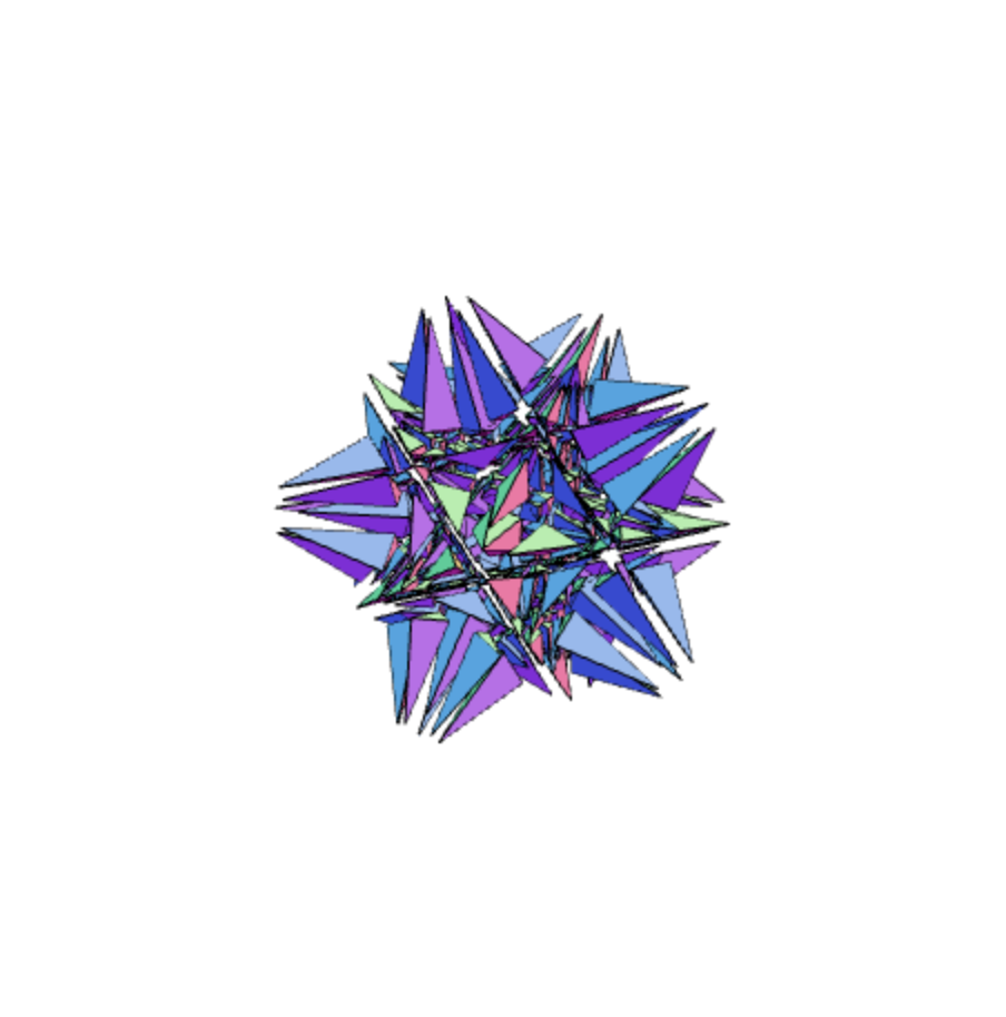
(a) $m=1$

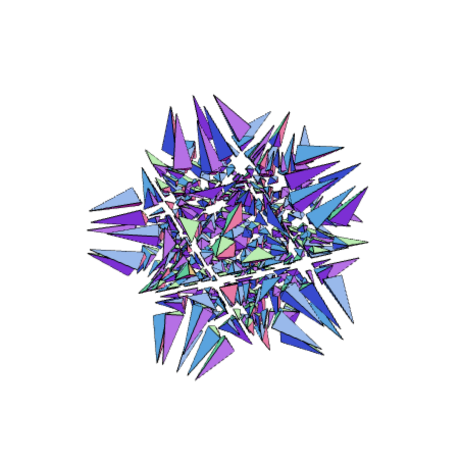
(b) $m=2$

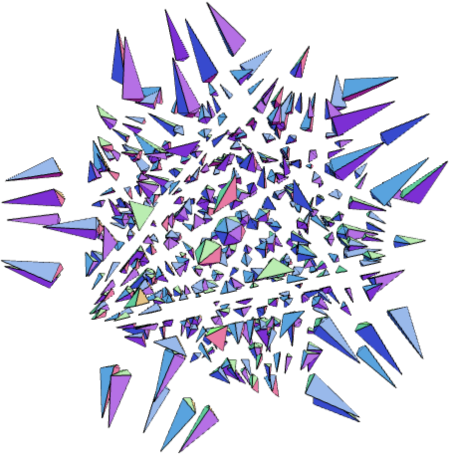
(c) $m=4$

Figure 8: Exploded Views of the $413$ internal Chambers of the Great Icosahedron with different Magnitudes $m$

The centre chamber of the great icosahedron is given by the regular icosahedron (a platonic solid).

Computing chambers and visualising them leads to a more profound understanding of the involved complexes. Volumes resp. other invariants can be computed in a parallel way for each chamber, leading to the volume resp. invariants of the whole given complex.

For example, consider the surface $X_{23}$, see [1], with symmetry group isomorphic to $C_{23}$ (cyclic group with $23$ elements). It has $6\cdot 23=138$ faces, $71$ vertices and $207$ edges with Euler characteristic $71-207+138=2$. Its symmetry group $G=\text{Sym}(X_{23})\leq\text{O}(3)$ is given by elements of the form

$$\begin{pmatrix}\cos(\varphi)&-\sin(\varphi)&0\\ \sin(\varphi)&\cos(\varphi)&0\\ 0&0&1\end{pmatrix}$$

with $\varphi\in\{\frac{2\pi\cdot j}{23}\mid 0\leq j<23\}$ and generated by

$$\begin{pmatrix}\cos(\frac{2\pi}{23})&-\sin(\frac{2\pi}{23})&0\\ \sin(\frac{2\pi}{23})&\cos(\frac{2\pi}{23})&0\\ 0&0&1\end{pmatrix}$$

which can be seen by matrix-multiplication and the addition theorem of $\cos$ and $\sin$. Label the $138$ faces $f_{1}$ to $f_{138}$, leading to $\binom{138}{2}=9453$ face pairs. There are exactly $6$ orbits of faces under the action of $G$, with representatives that we call $f^{\prime}_{1}$ to $f^{\prime}_{6}$. We can find all face pair intersections by the action of $G$ on pairs of the form $(f_{i}^{\prime},f),i=1,\dots,6$. Hence, it suffices to test intersection on these orbit representatives as every intersection can be obtained by applying a group element on one of these face pairs (see Section 5). We retriangulate $f_{1},\dots,f_{6}$ and then apply $G$ to obtain a retriangulation of the whole surface $X_{23}$. Transferring, i.e. applying group elements of $G$, can be done in linear time in the number of faces. Thus, we obtain an approximate speed-up in the order of $G$, so $23=|G|$. In Figure 9, we see an exploded view of the internal chambers of $X_{23}$.

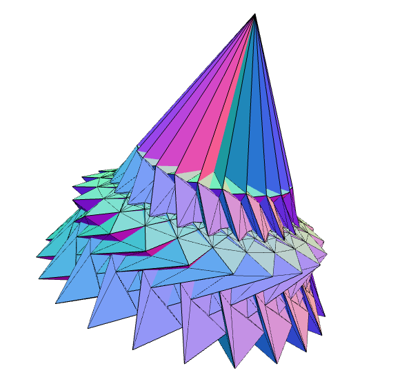
(a) $m=0$

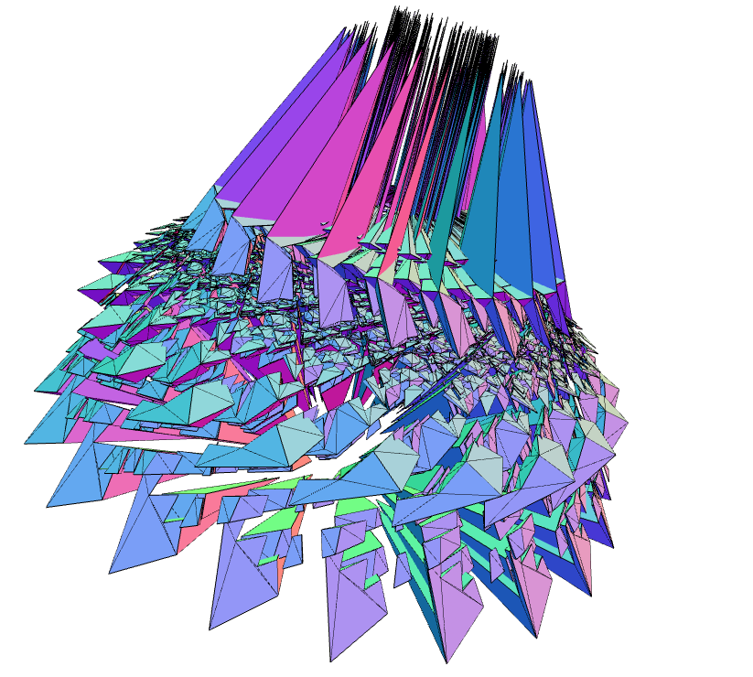
(b) $m=1$

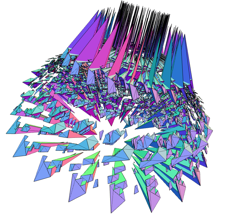
(c) $m=2$

Figure 9: Exploded Views of the Complex $X_{23}$ with different Magnitudes $m$

8 Ramifications

Another issue that might arise in a model is the existence of ramifications, that is non-manifold edges or non-manifold points. Remedying these non-manifold parts is crucial in many applications. In 3D-printing, for example, they cause problems or instabilities during the printing process, as a 3D printer can not print sets of zero measure. At the same time, they occur naturally, such as in the data set of embedded icosahedra of edge length one, see [6].
For efficiency reasons, it is sensible to consider these after first fixing self-intersections and computing the outer hull (for example, Figure 10 could be part of an inner chamber). Thus, in the following we assume a complex with embedding $(X,\phi)$ that is intersection-free and reduced to its outer hull.
Algebraically, the process of fixing non-manifold parts of a embedded complex corresponds to turning it into a simplicial surface by changing the parts that do not fulfil conditions $(i)$ and $(ii)$ from Definition 2.3.

Edge Ramifications

Non-manifold edges are edges which are incident to more than two triangles, as shown in Figure 10.

Figure 10: Red non-manifold Edge

We differentiate two types of non-manifold edges. Inner non-manifold edges are ones where both of its vertices are incident to another non-manifold edge, and outer non-manifold edges are ones where only one vertex is incident to another non-manifold edge.
We assume every non-manifold edge in our input to be connected to at least one other non-manifold edge. Since we already imposed closedness and reduction to the outer hull, only few irregular examples do not conform to this.
To correct a inner non-manifold edge $e$, we split vertices $v_{i}$ incident to $e$, resulting in new vertices $v^{j}_{i}$ for $i,j=1,2$. Additionally, we create another edge $e^{\prime}$ with $v^{2}_{1},v^{2}_{2}\in e^{\prime}$ and set $v^{1}_{1},v^{1}_{2}\in e$. The assignment of coordinates to the new vertices is decided based on the umbrellas.
For a outer non-manifold edge, we only split the vertex incident to another non-manifold edge. Both cases are visualised in Figure 11.

Figure 11: Splitting Ramified Edges based on Ramification Type: outer (left) and inner (right).

To compute the new vertices, we shift them by some $\varepsilon>0$ into a suitable direction $s_{e}$ given as follows.
For this $s_{e}$, choose faces $f_{1},f_{2}\supset e$ by taking $f_{1}\supset e$ and $f_{2}$ the next face on the fan of $e$ along the (correctly oriented) normal vector $n_{f_{1}}$ of $f_{1}$. We impose a compatibility condition,

$$\det[v,e,n_{f_{1}}]>0,$$

where $v$ is the vector orthogonal to $e$ pointing towards the vertex of $f_{1}$ not incident to e. This guarantees that we choose compatible directions $s_{e}$ for all non-manifold edges $e$. Then, take for both $f_{1},f_{2}$ the vertex $w_{i}$ that is not incident to $e$ and set

$$s_{e}:=1/2(w_{1}-v_{1})+1/2(w_{2}-v1).$$

Finally, we distribute the faces to the edges in such a way that the surface keeps being locally connected even after a cut, as seen in Figure 12.

Figure 12: Unramification of red Edge

This is embedded in a path-based framework: we first gather all the non-manifold edges and then treat edge-paths of non-manifold edges (which we call non-manifold paths) iteratively as described above. Every non-manifold path that is not a circle starts and ends at an outer non-manifold edge, and thus we only need to split one vertex per edge. For circles, it is also enough to split one vertex per edge and stop after reaching the first edge again.
If, while finding the non-manifold paths of the surface, there is a junction, it is sufficient to just choose one way and split the other ones up into disjoint paths, since the edges are already fixed by splitting the common vertex. It possible in certain configurations to produce a single ramified vertex after all ramified edges are corrected, which is why one should deal with edges first and then consider vertices.

Vertex Ramifications

Non-manifold points are ones at which the umbrella condition does not hold. So a neighbourhood of the point in the surface would fail to be connected if we would removed the point.
To remedy such a vertex $v_{0}$, we iterate over all local umbrellas $C_{\alpha}$ of $v$, that is all faces of $v$ that are edge-connected via edges that are incident to $v$. For each $C_{\alpha}$, we take for all $f\in C_{\alpha}$ their vertices $v_{f}^{1}$ and $v_{f}^{2}$ that do not equal $v_{0}$ and compute an average direction vector

$$p_{\alpha}=\dfrac{1}{|C_{\alpha}|}\left(\sum_{f\in C_{\alpha}}^{n}\dfrac{1}{2}(v_{f}^{1}-v_{0})+\dfrac{1}{2}(v_{f}^{2}-v_{0})\right).$$

Then, we replace $v_{0}$ by $v_{\alpha}:=v_{0}+p_{\alpha}\cdot\varepsilon$ in all of the $f$, where $\varepsilon>0$ is a small shift parameter.
Thus we move $v_{0}$ slightly in the direction of the local umbrella, and by doing this for each of the local umbrellas, we obtain $m$-moved versions of $v_{0}$ that are pairwise distinct and not non-manifold, where $\alpha=1,...,m$ is the number of $v$-edge-connected components of faces of $v$.
Lastly, for each $\alpha$, we exchange $v_{0}$ for $v_{\alpha}$ so that no new intersections or non-manifold vertices are created.

9 Self-Intersecting Icosahedra

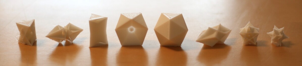
Figure 13: 3D-printed Icosahedra with Edge Length $2\text{cm}$

In [6], the authors classify all $35$ symmetric embeddings of icosahedra with equilateral triangles of edge length $1$. This means that the underlying simplicial surface agrees but the embedding varies, see [5] for coordinates and visualizations of the resulting surfaces. From these $35$ embeddings, $33$ have self-intersections and thus yield candidates for testing the algorithms presented in the previous sections.

In Figure 8, we see such an icosahedra, also known as great icosahedron, with automorphism group isomorphic to the whole icosahedral group. Thus, we can use symmetric optimzation as proposed in Section 5. In Table 1 we see that this leads to a large speed up of the factor $14.68$ when first retriangulating the surface and subsequently computing the outer hull. In Figure 13 we see printed versions of some of the icosahedra at edge length 2 cm.

The computations were performed on a MacBook Pro with Apple M1 Pro chip and 16GB memory averaging over 10 run times. We observe a strong correlation between the group sizes and the average speedup when comparing the time needed with or without using the symmetry group. In total, using the values given in Table 1, we have a speedup of a factor of approximately $3.17$.

10 Conclusion and Outlook

As can be seen from Table 1, for a group size of 2, which corresponds to just a single symmetry in the model, the average speedup in our data set is still $2.12$. Thus, even if no symmetries are known a-priori, symmetry detection as in [15] and [7] can be used to compute the automorphism group and employ a symmetry-driven algorithm such as ours. If symmetries are already given, the advantage are even bigger. The symmetry optimisation method can be also applied to infinite structures if the face-orbits are finite. For instance, crystallographic groups give examples of doubly periodic symmetries with face-orbit representatives sitting inside a fundamental domain, see [13, 24] for examples of such surfaces.
The study of chambers of an embedded complex can be used to compute various geometric properties such as volume and has the potential of designing interlocking puzzles [9] by subdividing a given complex into its chambers and introduce connectors.

The retriangulation method in this paper is motivated by producing a complex with a minimal number of triangles. The robustness of the underlying algorithm and the possibility of applying symmetries leads to a numerical stable and fast method. The results we obtained for embedded icosahedra and cyclic complexes show that a high order of speedup is possible without any loss of algorithmic stability.
It would also be possible to for example study modifications that enhance the run time both theoretically and for practical examples as follows. The outer hull algorithm given by [2] is applied to obtain the outer hull of the retriangulated complex (after removing self-intersection) and further studied in the context of chambers. Additionally, one could consider finding alternative algorithms that compute the outer hull before considering self-intersections, since only the ones one the outer hull are relevant in many settings. For practical reason, e.g. 3D-printing of surfaces, we consider rectification of complexes to obtain 3D-printable files. In this context non-manifold parts are replaced or adjusted. Non-manifold edges (also known as ramified edges) are considered and replaced to gain a surface that is as close as possible to the initial surface while yielding a 3D-printable file. Future research needs to be conducted to gain an understanding of how parameters need to be set in order to guarantee a model that satisfies the same properties as the underlying geometric model.

11 Acknowledgments

This work was funded by the Deutsche Forschungsgemeinschaft (DFG, German Research Foundation) - SFB/TRR 280. Project-ID: 417002380. The authors thank Prof. Alice C. Niemeyer for her valuable comments and Lukas Schnelle for support in generation of images.

12 Appendix

Table 1: Timing of computing outer hull of Icosahedra [5]

Icosahedron	Group Size	Time w/ Group (ms)	Time w/ Group (ms)	Speedup
Icosahedron_1_1	4	30.6	83.0	2.71
Icosahedron_2_1	120	715.4	10502.6	14.68
Icosahedron_2_2	120	13.6	67.4	4.96
Icosahedron_3_1	20	75.0	385.6	5.14
Icosahedron_3_2	20	280.8	116.0	3.80
Icosahedron_4_1	12	35.8	80.9	2.31
Icosahedron_4_2	12	84.9	424.1	2.26
Icosahedron_5_1	4	33.2	144.7	5.00
Icosahedron_5_2	4	116.0	622.1	4.36
Icosahedron_6_1	20	39.2	140.6	5.36
Icosahedron_7_1	12	1090.5	2536.7	2.33
Icosahedron_7_2	12	488.8	1343.2	2.75
Icosahedron_7_3	12	212.8	517.5	2.43
Icosahedron_8_1	4	111.5	325.1	2.92
Icosahedron_9_1	4	229.8	409.1	1.78
Icosahedron_9_2	4	2074.3	4097.2	1.98
Icosahedron_9_3	4	89.8	149.2	1.66
Icosahedron_9_4	4	136.8	241.9	1.77
Icosahedron_9_5	4	58.3	99.3	1.70
Icosahedron_10_1	2	679.9	3024.7	4.45
Icosahedron_10_2	2	21.2	66.9	3.16
Icosahedron_11_1	10	99.1	248.1	2.50
Icosahedron_11_2	10	42.6	111.6	2.62
Icosahedron_12_1	6	137.9	213.0	1.54
Icosahedron_12_2	6	109.7	163.8	1.49
Icosahedron_12_3	6	145.9	240.3	1.65
Icosahedron_12_4	6	223.2	380.5	1.70
Icosahedron_13_1	2	352.8	567.4	1.61
Icosahedron_13_2	2	751.4	1130.4	1.50
Icosahedron_13_3	2	460.7	703.2	1.53
Icosahedron_13_4	2	467.0	780.6	1.67
Icosahedron_13_5	2	153.2	236.4	1.54
Icosahedron_13_6	2	243.9	373.4	1.53
Icosahedron_14_1	10	57.3	182.9	3.19

References

- [1] Reymond Akpanya and Tom Goertzen “Surfaces with given Automorphism Group” In arXiv e-prints, 2023, pp. arXiv:2307.12681 DOI: 10.48550/arXiv.2307.12681
- [2] Marco Attene “As-exact-as-possible repair of unprintable STL files” In Rapid Prototyping Journal 24.5 Emerald Publishing Limited, 2018, pp. 855–864 DOI: 10.1108/RPJ-11-2016-0185
- [3] Marco Attene “Direct repair of self-intersecting meshes” In Graphical Models 76.6, 2014, pp. 658–668 DOI: https://doi.org/10.1016/j.gmod.2014.09.002
- [4] Markus Baumeister “Regularity aspects for combinatorial simplicial surfaces”, 2020 DOI: 10.18154/RWTH-2020-07027
- [5] Karl-Heinz Brakhage et al. “Documentation of Paper: The icosahedra of edge length 1” (Accessed on 30/11/2023), http://algebra.data.rwth-aachen.de/Icosahedra/visualplusdata.html
- [6] Karl-Heinz Brakhage et al. “The icosahedra of edge length 1” In J. Algebra 545, 2020, pp. 4–26 DOI: 10.1016/j.jalgebra.2019.04.028
- [7] Mladen Buric, Tina Bosner and Stanko Skec “A Framework for Detection of Exact Global and Partial Symmetry in 3D CAD Models” In Symmetry 15.5, 2023 DOI: 10.3390/sym15051058
- [8] Marcel Campen and Leif Kobbelt “Exact and Robust (Self-)Intersections for Polygonal Meshes” In Computer Graphics Forum 29.2, 2010, pp. 397–406 DOI: https://doi.org/10.1111/j.1467-8659.2009.01609.x
- [9] Rulin Chen, Ziqi Wang, Peng Song and Bernd Bickel “Computational Design of High-Level Interlocking Puzzles” In ACM Trans. Graph. 41.4 New York, NY, USA: Association for Computing Machinery, 2022 DOI: 10.1145/3528223.3530071
- [10] Lei Chu, Hao Pan, Yang Liu and Wenping Wang “Repairing Man-Made Meshes via Visual Driven Global Optimization with Minimum Intrusion” In ACM Trans. Graph. 38.6 New York, NY, USA: Association for Computing Machinery, 2019 DOI: 10.1145/3355089.3356507
- [11] Leila De Floriani, Daniele Panozzo and Annie Hui “Computing and Visualizing a Graph-Based Decomposition for Non-manifold Shapes” In Graph-Based Representations in Pattern Recognition Berlin, Heidelberg: Springer Berlin Heidelberg, 2009, pp. 62–71 DOI: 10.1007/978-3-642-02124-4_7
- [12] “GAP – Groups, Algorithms, and Programming, Version 4.12.2”, 2022 The GAP Group URL: https://www.gap-system.org
- [13] Tom Goertzen, Alice C. Niemeyer and Wilhelm Plesken “Topological Interlocking via Symmetry” In 6th fib International Congress on Concrete Innovation for Sustainability, 2022; Oslo; Norway, 2022, pp. 1235–1244 URL: https://www.scopus.com/inward/record.uri?eid=2-s2.0-85143905977&partnerID=40&md5=157f82e57ed12d582902da55864644a7
- [14] Aleksey Golovinskiy and Thomas Funkhouser “Consistent Segmentation of 3D Models” In Computers and Graphics (Shape Modeling International 09) 33.3, 2009, pp. 262–269
- [15] Bo Li, Henry Johan, Yuxiang Ye and Yijuan Lu “Efficient 3D reflection symmetry detection: A view-based approach” SIGGRAPH Asia Workshop on Creative Shape Modeling and Design In Graphical Models 83, 2016, pp. 2–14 DOI: https://doi.org/10.1016/j.gmod.2015.09.003
- [16] Yijing Li and Jernej Barbič “Immersion of Self-Intersecting Solids and Surfaces” In ACM Trans. Graph. 37.4 New York, NY, USA: Association for Computing Machinery, 2018 DOI: 10.1145/3197517.3201327
- [17] Conor Mccoid and Martin J. Gander “A Provably Robust Algorithm for Triangle-Triangle Intersections in Floating-Point Arithmetic” In ACM Trans. Math. Softw. 48.2 New York, NY, USA: Association for Computing Machinery, 2022 DOI: 10.1145/3513264
- [18] Tomas Möller “A Fast Triangle-Triangle Intersection Test” In Journal of Graphics Tools 2.2 Taylor & Francis, 1997, pp. 25–30 DOI: 10.1080/10867651.1997.10487472
- [19] Alice C. Niemeyer, Wilhelm Plesken and Daniel Robertz “Simplicial Surfaces of Congruent Triangles” In preparation, 2023
- [20] Jarek Rossignac and David Cardoze “Matchmaker: Manifold BReps for Non-Manifold r-Sets” In Proceedings of the Fifth ACM Symposium on Solid Modeling and Applications, SMA ’99 Ann Arbor, Michigan, USA: Association for Computing Machinery, 1999, pp. 31–41 DOI: 10.1145/304012.304016
- [21] Vaclav Skala “A Brief Survey of Clipping and Intersection Algorithms with a List of References (including Triangle-Triangle Intersections)” In Informatica 34.1 Vilnius University, 2023, pp. 169–198 DOI: 10.15388/23-INFOR508
- [22] John Vince “Geometry for Computer Graphics: Formulae, Examples and Proofs” Published: 05 January 2005 Springer London, 2005, pp. XXII\bibrangessep342 DOI: 10.1007/b138852
- [23] Marc Wagner, Ulf Labsik and Günther Greiner “Repairing non-manifold triangle meshes using simulated annealing” In International Journal of Shape Modeling 9, 2003 DOI: 10.1142/S0218654303000085
- [24] Sebastian Wiesenhuetter et al. “Triply Periodic Minimal Surfaces – A Novel Design Approach for Lightweight CRC Structures” In Building for the Future: Durable, Sustainable, Resilient Cham: Springer Nature Switzerland, 2023, pp. 1449–1458 URL: https://doi.org/10.1007/978-3-031-32511-3_148
- [25] “Writing an .stl file from scratch” (Accessed on 01/12/2023), https://danbscott.ghost.io/writing-an-stl-file-from-scratch/
- [26] Soji Yamakawa and Kenji Shimada “Removing Self Intersections of a Triangular Mesh by Edge Swapping, Edge Hammering, and Face Lifting” In Proceedings of the 18th International Meshing Roundtable Berlin, Heidelberg: Springer Berlin Heidelberg, 2009, pp. 13–29
- [27] Jiang Zhu, Yurio Hosaka and Hayato Yoshioka “A Robust Algorithm to Remove the Self-intersection of 3D Mesh Data without Changing the Original Shape” In Journal of Physics: Conference Series 1314.1 IOP Publishing, 2019, pp. 012149 DOI: 10.1088/1742-6596/1314/1/012149