Golden parachutes under the threat of accidents

Abstract

This paper addresses a continuous-time contracting model that extends the problem introduced by Sannikov [47] and later rigorously analysed by Possamaï and Touzi [44]. In our model, a principal hires a risk-averse agent to carry out a project. Specifically, the agent can perform two different tasks, namely to increase the instantaneous growth rate of the project’s value, and to reduce the likelihood of accidents occurring. In order to compensate for these costly actions, the principal offers a continuous stream of payments throughout the entire duration of a contract, which concludes at a random time, potentially resulting in a lump-sum payment. We examine the consequences stemming from the introduction of accidents, modelled by a compound Poisson process that negatively impact the project’s value. Furthermore, we investigate whether certain economic scenarii are still characterised by a golden parachute as in Sannikov’s model. A golden parachute refers to a situation where the agent stops working and subsequently receives a compensation, which may be either a lump-sum payment leading to termination of the contract or a continuous stream of payments, thereby corresponding to a pension.

Key words: principal–agent problem, random horizon, integro-differential Hamilton–Jacobi–Bellman equation

1 Introduction

Risk naturally emerges in various interactions across all sectors of the economy and is well-known to be closely linked to the concept of uncertainty. It involves the potential occurrence of unexpected shocks that could lead to harm or loss, thus exerting a significant—and usually negative—influence on the considered economic scenario. Here, one is naturally led to consider situations such as accidents during the production process in a company, injuries in an health insurance context, or even the devaluation of financial assets in specific corporations, due to the bankruptcy of a subsidiary. Although various other instances could be mentioned, they all have in common the potential for certain adverse events that can be categorised as accidents. It is therefore natural to study risk prevention in contract theory, specifically within principal–agent problems.

The principal–agent paradigm addresses the optimal contracting problem in the presence of information asymmetry between two economic actors: a principal (‘she’) and an agent (‘he’). In the typical scenario, the principal designs a contract to hire the agent, who can accept or reject it based on whether it provides sufficiently adequate incentives to ensure that his reservation utility is attained. The primary challenge is that the principal designs this contract to optimise her utility while having imperfect information about the efforts provided by the agent. This problem originated in the 1970s within a discrete-time framework and was subsequently reformulated in a continuous-time model by Holmström and Milgrom [26]. This seminal work initiated the study of moral hazard problems in continuous-time, providing important insights into formulating an optimal contract between a principal and an agent whose effort influences the drift of the output process. Following this, numerous results have been established to explore more general models and derive tractable solutions, thereby expanding the scope of this initial work. A comprehensive analysis of the related literature can be found in the survey paper of Sung [55] or in the book of Cvitanić and Zhang [18].

It has nowadays been universally acknowledged that Sannikov [47] achieved a substantial breakthrough in the field. In this work, the author studied an infinite horizon principal–agent model, in which the principal provides continuous payments to the agent, who exclusively controls the drift of the output process until a random retirement time. The significance of this work lies in its pioneering approach, which enables the transformation of the original bi-level optimisation problem between the principal and the agent into a standard stochastic control problem, whose solution can be described through an Hamilton–Jacobi–Bellman equation. This approach led to numerous follow-up works that rigorously formalised Sannikov’s ideas. Particularly noteworthy are the PhD thesis of Choi [13] and, more recently, the contribution of Possamaï and Touzi [44], which extended the principal–agent model introduced by Sannikov by considering potentially different discount rates for both parties. Their primary focus was on technical rigour, ultimately providing a complete characterisation of the solution to the contracting problem. Another significant extension was introduced by Cvitanić, Possamaï, and Touzi [19], presenting a comprehensive mathematical approach to solve principal–agent problems that allow control over both the drift and diffusion of the output process. While this analysis focused on a finite deterministic horizon setting, Lin, Ren, Touzi, and Yang [33] subsequently addressed principal–agent problems over random horizons.

It is nonetheless important to point out that the Brownian framework considered in all the previously mentioned works fails to capture sudden and unpredictable events, and consequently it becomes necessary to consider principal–agent problems involving a jump component in the output process. There exists a vast literature that adopts jump processes to replicate negative shocks, with an early influential contribution from Sung [54]. This work extended Holmström and Milgrom’s model, addressing a corporate insurance problem driven by a multi-dimensional point process, where each component represents a specific type of accident, less likely to occur when the agent exerts effort. More recently, Zhang [56] explored efficient allocations in a Mirrleesean economy influenced by persistent shocks that transition according to a continuous-time Markov chain that is beyond the control of the agent. Similarly, Sannikov and Skrzypacz [48] investigated the dynamic interaction among economic actors in a scenario where the information process is characterised by a discontinuous uncontrolled Poisson component associated to bad news. In contrast, Biais, Mariotti, Rochet, and Villeneuve [9, 10] simulated accidents and large and unfrequent losses, respectively, using a Poisson process whose intensity can be influenced by the agent’s actions. Additionally, Pagès and Possamaï [40], later extended by Hernández Santibáñez, Possamaï, and Zhou [24] to include adverse selection, explored the optimal securitisation of a pool of long-term loans exposed to Poisson default risk, where the default intensity can be reduced through the monitoring activity of a bank. Furthermore, Martin and Villeneuve [36] modelled a large insurable risk capable of halting production entirely using a single jump process. However, it is worth noting that in existing literature, a jump process is not exclusively associated with negative events. El Euch, Mastrolia, Rosenbaum, and Touzi [21] linked a Poisson process with market orders to investigate a contract offered by an exchange to a market-maker, aiming to reduce the bid–ask spread for a single risky asset. Subsequently, this model was extended to consider multiple market participants by Baldacci, Possamaï, and Rosenbaum [4] and to enable trading on dark liquidity pools by Baldacci, Manziuk, Mastrolia, and Rosenbaum [5].

All the previously mentioned works adopt jump processes with a constant jump size to simulate sudden shocks. To the best of our knowledge, the first study to consider accidents of different random sizes is by Capponi and Frei [12]. The authors examined a principal–agent model where the agent can exert both effort and accident prevention, aiming to decrease the likelihood of negative events that are described by an exogenous loss distribution. Later on, Bensalem, Hernández Santibáñez, and Kazi-Tani [8] employed a similar jump–diffusion framework in their investigation of an insurance demand model, enabling the protection buyer to exert prevention effort to reduce his risk exposure. An extension of all the aforementioned principal–agent models can be found in the work of Hernández Santibáñez [23]. Here, the author studied a general contracting problem between the principal and a finite number of agents, where each agent has control over the drift of the output process and the compensator of its associated jump measure. Additionally, Mastrolia and Zhang [37] formulated an energy-optimal demand–response model where the principal hires an infinite number of agents, incorporating accidents by introducing a Lévy process.

Principal–agent models with jumps that go beyond simple Poisson process lead to Hamilton–Jacobi–Bellman equations with an additional integral term. Consequently, the notion of viscosity solution introduced by Crandall and Lions [16] and Lions [35] requires particular attention as the equations become non-local. The first works in this direction are to be attributed to Soner [52, 53] for bounded measures and Sayah [49, 50] for unbounded measures. Subsequently, Alvarez and Tourin [2] proved a general existence and uniqueness result for viscosity solutions to integro-differential equations characterised by a bounded integral operator, while Pham [42] achieved a similar result for a special case involving singular measures. In recent years, there has been a surge of interest in extending the theory of viscosity solutions to integro-differential equations. This growth in the literature is largely due to the dependence of the results on the integrability of the singular measure characterising the integral operator. Among these advancements, Jakobsen and Karlsen [28] presented a first version of a non-local maximum principle, which allowed the deduction of a comparison principle for viscosity sub-quadratic solutions. Subsequently, Barles and Imbert [7] and later the PhD thesis of Hollender [25] generalised their uniqueness result by considering solutions with arbitrary growth at infinity.

In this paper, we examine the model introduced by Sannikov [47] in the presence of accidents, thereby making the model suitable for investigating contracting problems between a principal and an agent in an economic environment that might experience unpredictable and negative shocks of unknown size. Specifically, we explore optimal contracts offered by a risk-neutral principal to a risk-averse agent aimed at executing a project. To maximise the project’s value, which is described by an underlying jump–diffusion process, the agent can employ two distinct actions simultaneously, influencing both the drift of the process and the likelihood of accidents occurring. We model the impact of accidents using a compound Poisson process, in line with the approach outlined by Capponi and Frei. However, a slight issue arises in the derivation of optimal contracts in the mentioned work, particularly in the application of the martingale representation property in [12, Lemma 3.1]. This issue inevitably imposes a restriction on the set of the admissible contracts. Consequently, our contribution can be seen as an extension to this model, not only due to this concern but also because we assume that the principal offers compensation to the agent not solely at the random termination time but consistently throughout the entire duration of the contract.

The main objective of this paper is to verify whether the rigorous study by Possamaï and Touzi [44] regarding Sannikov’s contracting problem remains valid within our framework that incorporates accidents. More specifically, we aim to test the robustness of the economic conclusions drawn by these authors by studying the economic implications resulting from these unpredictable events that negatively impact the principal–agent interaction. Our focus is particularly on examining the concept of a ‘golden parachute’ in the context of accident risk. This term refers to a situation where the agent ceases to work at a random time—or refrains from working completely—and subsequently receives a positive compensation. This compensation may take the form of a lump-sum payment, leading to termination of the contract, or a continuous stream of payments, indicating retirement. Therefore, our investigation aims to determine whether economic conditions exist that could lead to the existence of these two distinct instances of golden parachutes, similarly to what was observed in the problem without accidents. To conduct this analysis, we need to consider different regimes based on the impatience levels of both parties:

1. when the principal is significantly more impatient than the agent, a golden parachute does not exist. This scenario depends only on the impatience of both economic actors and the agent’s level of risk aversion, completely mirroring the case without accident risk. Indeed, the problem degenerates because the principal can achieve her maximum reward regardless of the agent’s participation level. However, optimal contracts do not exist;

2. when the principal is more impatient than the agent but still above the threshold mentioned above, a golden parachute can correspond to either of the previously described situations. Unlike the analysis not involving accidents, if the agent stops working, this means that he is either fired or retired. This difference is due to the impact of accidents on the economic scenario, leading the principal to prefer terminating the contract over retiring the agent for a sufficiently small continuation utility of the agent. This decision is influenced by the expenses associated with potential future losses outweighing the immediate cost of compensating the agent. This is in stark contrast with the analysis excluding accidents, where termination is never considered the optimal choice;

3. when the principal is as impatient as the agent, the analysis closely aligns with that conducted without considering accidents. In other words, we know that a golden parachute is likely to exist, and it corresponds to a lump-sum compensation;

4. when the agent is strictly more impatient than the principal, a golden parachute can be associated with both distinct compensation schemes, which further depends on the average loss per accident. When the size of potential accidents is not significant, contract termination is never an optimal choice, analogously to the model without accidents. However, when the impact of an accident grows significantly, resulting in higher associated costs, the principal prefers either firing the agent or retiring him, based on the continuation utility of the agent. Hence, we observe that the nature of a golden parachute is deeply linked to the average accident size. In case of large accidents, it translates to either a lump-sum payment or a continuous stream of payments. Conversely, as the accident size decreases, it corresponds to the retirement scenario, mirroring the situation in the absence of accidents.

We emphasise that the economic features of the model are closely related to the specific regime under consideration and thus rely on the impatience levels of both parties, exactly as in the problem without accidents. However, despite the unchanged structure of the problem, the introduction of unpredictable and adverse events allows for the possibility of both golden parachute scenarii. In other words, when the agent is not as impatient as the principal, a golden parachute can be associated with both retirement and termination, while retirement is always the preferred choice in the absence of accidents. This different characterisation stems from the different nature of an appropriate face-lifted version of the agent’s inverse utility function, which is defined through an obstacle problem. While in the accident-free framework, this problem simplifies to the study of an ordinary differential equation, in our model, the analysis of this face-lifted utility function is significantly more involved due to its significant correlation with the average accident size. We also mention that even with relatively small potential accidents, the impact on the principal is significant, and can result in a 50% reduction of the value of the principal for an accident size which represents only 2.5% of the average value of the project.

Another important difference with the reference model without accidents is obvious in the study of the first-best problem, which is no longer directly solvable, except in the scenario where the principal and the agent are equally impatient. Despite the difficulty in fully characterising the first-best solution for every regime, we can still replicate similar economic considerations. However, the most challenging aspect of investigating the model incorporating accidents lies in describing the second-best problem in order to address the economic question of whether a golden parachute is optimal. Unfortunately, we cannot provide a definitive answer to this question due to the complexity arising from the integral term appearing in the Hamilton–Jacobi–Bellman equation associated with the contracting problem. We will discuss this in more detail in Section 5.2. Nonetheless, we are able to characterise the solution to the problem as the unique viscosity solution of the aforementioned equation through a generalisation of Tietze’s extension theorem that allows to overcome the obstacles posed by the limited liability constraint.

The rest of the paper is structured as follows. In Section 2, we formulate the principal–agent model and provide a comprehensive explanation of the criteria of the agent and the principal. We then discuss the two notions of a golden parachute along with the definition of the face-lifted utility function that combines these concepts. In Section 3, we completely characterise the face-lifted utility in all the various cases $(i)$, $(ii)$, $(iii)$ and $(iv)$ outlined above. In Section 4, we study the first-best contracting problem, which offers insights into the subsequent analysis of the second-best contracting problem in Section 5. We defer technical proofs to the appendices.

Notation. Let $\mathbb{N}$ be the set of positive integers, and $\mathbb{R}_{+}$ the set of non-negative real-numbers. For any $(a,b)\in[-\infty,\infty]^{2}$, we write $a\wedge b\coloneqq\min\{a,b\}$ and $a\vee b\coloneqq\max\{a,b\}$. Consider a probability space $(\Omega,\mathcal{F},\mathbb{P})$ carrying a filtration $\mathbb{F}\coloneqq(\mathcal{F}_{t})_{t\geq 0}$. We use the convention $\mathcal{F}_{0-}\coloneqq\mathcal{F}_{0}$ and $\mathcal{F}_{\infty}\coloneqq\mathcal{F}_{\infty-}\coloneqq\sigma(\cup_{t\geq 0}\mathcal{F}_{t})$. For $t\in[0,\infty]$, we write $\mathbb{E}^{\mathbb{P}}_{t}[\xi]$ for the conditional expectation of a random variable $\xi$ with respect to $\mathcal{F}_{t}$. For any $\mathbb{F}$–stopping time $\tau$, we denote by $\mathcal{T}_{\tau}(\mathbb{F})$ the set of $\mathbb{F}$–stopping times $\theta$ such that $\theta\leq\tau$, $\mathbb{P}$–a.s., and by $\llbracket\theta,\tau\rrbracket$ (resp. $\rrbracket\theta,\tau\rrbracket$) the stochastic interval $\{(t,\omega)\in\mathbb{R}_{+}\times\Omega:\;\theta(\omega)\leq(\text{resp.}<)\;t\leq\tau(\omega)\}$. The notation $\widetilde{\mathcal{P}}(\mathbb{F})$ (resp. $\widetilde{\mathcal{O}}(\mathbb{F})$) refers to the predictable (resp. optional) $\sigma$-algebra on $\Omega\times\mathbb{R}_{+}\times\mathbb{R}$. For a random measure $\mu$ on $\mathbb{R}_{+}\times\mathbb{R}$, we denote by $\mu^{p}$ (resp. $\tilde{\mu}\coloneqq\mu-\mu^{p}$) its $(\mathbb{F},\mathbb{P})$-compensator (resp. $(\mathbb{F},\mathbb{P})$-compensated random measure). We introduce the spaces

$$G_{\rm loc}(\mu,\mathbb{F},\mathbb{P}) \coloneqq\bigg{\{}\mathbb{R}\text{\rm-valued},\;\widetilde{\mathcal{P}}(\mathbb{F})\text{\rm-measurable functions}\;U:\bigg{(}\int_{0}^{\cdot}\int_{\mathbb{R}}|U_{s}(\ell)|^{2}\mu(\mathrm{d}s,\mathrm{d}\ell)\bigg{)}^{\frac{1}{2}}\;\text{\rm is}\;(\mathbb{F},\mathbb{P})\text{\rm--locally}\;\mathbb{P}\text{\rm-{integrable}}\bigg{\}},\;$$

$$\mathbb{L}^{2}_{\mathrm{loc}}(W,\mathbb{F},\mathbb{P}) \coloneqq\bigg{\{}\mathbb{R}\text{\rm-valued},\;\mathbb{F}\text{\rm-predictable processes}\;Z:\int_{0}^{\cdot}|Z_{s}|^{2}\mathrm{d}s\;\text{\rm is}\;(\mathbb{F},\mathbb{P})\text{\rm--locally}\;\mathbb{P}\text{\rm-integrable}\bigg{\}},$$

where $W$ is an $(\mathbb{F},\mathbb{P})$–Brownian motion. For an $(\mathbb{F},\mathbb{P})$–local martingale $X$ in the sense of Jacod and Shiryaev [27, Definition I.1.45], we denote its stochastic exponential by $\mathcal{E}(X)$, that is,

$$\mathcal{E}(X)_{t}=\mathrm{exp}\big{(}X_{t}-\frac{1}{2}[X^{c}]_{t}\big{)}\prod_{0<s\leq t}(1+\Delta X_{s})\mathrm{e}^{-\Delta X_{s}},\;\text{for}\;t\geq 0,$$

where $[X^{c}]$ is the quadratic variation of the continuous martingale part of $X$ and $\Delta X$ denotes the jump process of $X$ (as in [27, Theorem I.4.61]).

2 Model and assumptions

We investigate a continuous-time contracting problem in which a risk-neutral principal hires a risk-averse agent to manage a project over a possibly infinite time horizon. During this period, the agent can exert effort to increase the instantaneous growth rate of the project’s value, that is, the principal’s profit, while simultaneously reducing the likelihood of accidents that negatively impact the total profit. It is important to emphasise that in the model considered here, the agent is unable to reduce the impact of accidents on the project’s value as he has no control over their size, which is an exogenous factor.

2.1 The setting

Let $\left(\Omega,\mathcal{F},\mathbb{P}\right)$ be a probability space carrying the following jointly $\mathbb{P}$–independent objects: a one-dimensional Brownian motion $W=(W_{t})_{t\geq 0}$, a Poisson process $N=(N_{t})_{t\geq 0}$ with $\mathbb{P}$-intensity $\int_{0}^{\cdot}\mathrm{d}s$ (see [27, Definition I.3.26]), and a collection of bounded and positive $\mathbb{P}$–i.i.d. random variables $(L_{i})_{i\in\mathbb{N}}$. Let $\sigma>0$, and let $x_{0}\in\mathbb{R}$ denote a given initial investment. The dynamics of the project’s value, referred to as the output process hereafter, under no exertion of effort by the agent is given by

$$X_{t}\coloneqq x_{0}+\sigma W_{t}-J_{t},\;\text{for}\;t\geq 0,$$

where $J=(J_{t})_{t\geq 0}$ denotes the compound Poisson process

$$J_{t}\coloneqq\sum_{i=1}^{N_{t}}L_{i},\;\text{for}\;t\geq 0.$$

Here, $W$ represents a source of randomness, and $J$ models the losses that can occur throughout the lifetime of the project at random times. The Poisson process $N$ represents the total number of accidents, while $J$ the respective cumulative losses since, for $i\in\mathbb{N}$, each random variable $L_{i}$ quantifies the size of the $i$-th accident. The average loss per accident is denoted by

$$m\coloneqq\mathbb{E}^{\mathbb{P}}[L_{i}]=\int_{\mathbb{R}_{\text{$+$}}}\ell\Phi(\mathrm{d}\ell),$$ (2.1)

where $\Phi$ is the common distribution function associated to all the $L_{i}$, $i\in\mathbb{N}$. Note that $m$ is positive since $L_{i}$ is assumed to be positive. Finally, we let $\mathbb{F}=(\mathcal{F}_{t})_{t\geq 0}$ be the $\mathbb{P}$-augmentation of the filtration generated by the Brownian motion $W$ and the compound Poisson process $J$. Note that $\mathbb{F}$ satisfies the usual conditions under $\mathbb{P}$ by Protter [45, Theorem I.31].

In this setting, a natural question to ask is whether the predictable martingale representation property with respect to $W$ and $J$ holds. This can indeed be achieved by introducing the associated jump measure of $J$ as follows. Let

$$\mu^{J}(\mathrm{d}t,\mathrm{d}\ell)\coloneqq\sum_{s>0}\mathbf{1}_{\{\Delta J_{\text{$s$}}\neq 0\}}\varepsilon_{(s,\Delta J_{\text{$s$}})}(\mathrm{d}t,\mathrm{d}\ell),$$

where $\varepsilon$ denotes the Dirac measure, the $(\mathbb{F},\mathbb{P})$-compensator (see [27, Theorem II.1.8] for the definition) is then given by

$$\mu^{J,p}(\mathrm{d}t,\mathrm{d}\ell)\coloneqq\Phi(\mathrm{d}\ell)\mathrm{d}t.$$

To ease the notation, we write $\tilde{\mu}^{J}(\mathrm{d}t,\mathrm{d}\ell)$ for the compensated random measure $\mu^{J}(\mathrm{d}t,\mathrm{d}\ell)-\mu^{J,p}(\mathrm{d}t,\mathrm{d}\ell)$. Furthermore, for any $Z\in\mathbb{L}^{2}_{\mathrm{loc}}(W,\mathbb{F},\mathbb{P})$ and $U\in G_{\rm loc}(\mu^{J},\mathbb{F},\mathbb{P})$, we denote by

$$\int_{0}^{t}Z_{s}\mathrm{d}W_{s}\;\text{and}\;\int_{0}^{t}\int_{\mathbb{R}}U_{s}(\ell)\tilde{\mu}^{J}(\mathrm{d}s,\mathrm{d}\ell),\;t\geq 0,$$ (2.2)

the stochastic integral of $Z$ with respect to $W$ and the compensated stochastic integral of $U$ with respect to the random measure $\mu^{J}$, respectively, in the sense of [27, Chapter 1 & 2]. Having collected the necessary ingredients, we can now state the following martingale representation theorem, which is derived from Cohen and Elliott [14, Theorem 14.5.7] combined with [27, Observation I.4.1].

Lemma 2.1.

Let $M$ be an $(\mathbb{F},\mathbb{P})$–local martingale. Then, there exist unique $Z\in\mathbb{L}^{2}_{\mathrm{loc}}(W,\mathbb{F},\mathbb{P})$ and $U\in G_{\rm loc}(\mu^{J},\mathbb{F},\mathbb{P})$ such that

$$M_{t}=M_{0}+\int_{0}^{t}Z_{s}\mathrm{d}W_{s}+\int_{0}^{t}\int_{\mathbb{R}}U_{s}(\ell)\tilde{\mu}^{J}(\mathrm{d}s,\mathrm{d}\ell),\;t\geq 0,\;\mathbb{P}\text{\rm--a.s.}$$

Moreover, this property is preserved under an equivalent change of measure, see for instance [27, Theorem III.5.24].

2.2 Actions and contracts

We assume that through specific costly efforts, the agent can influence the distribution of the output process $X$, that is, he can affect the probability measure under which the problem is described in its weak formulation. For this, we introduce a compact subset $A$ of $\mathbb{R}_{+}$ containing $0$ and bounded by $\bar{a}\in A$, for some $\bar{a}>0$, representing the possible effort values that the agent can exert on the drift of the output process. Additionally, we define another compact subset $B$ of $\mathbb{R}_{+}$ bounded by $m$. This set $B$ denotes all possible accident frequencies, which is why it needs to satisfy the technical condition of being bounded away from zero. Specifically, there exists some $\varepsilon_{m}\in B$ such that $\varepsilon_{m}\in(0,m]$ and $\varepsilon_{m}\leq b$ for any $b\in B$. Note that the fact that $\varepsilon_{m}$ is positive implies that accidents are less likely to happen if the agent exerts effort, but he cannot eliminate them completely. We denote for simplicity $U\coloneqq A\times B$.

The collection of admissible controls $\mathcal{U}$ for the agent consists of all $\mathbb{F}$-predictable processes $\nu\coloneqq(\alpha,\beta)$ with values in $U$ such that the following stochastic exponential

$$M^{\nu}_{t}\coloneqq\mathcal{E}\left(\int_{0}^{\cdot}\frac{\alpha_{s}}{\sigma}\mathrm{d}W_{s}\right)_{t}\mathcal{E}\left(\int_{0}^{\cdot}\left(\frac{\beta_{s}}{m}-1\right)\left(\mathrm{d}N_{s}-\mathrm{d}s\right)\right)_{t}=\mathcal{E}\bigg{(}\int_{0}^{\cdot}\frac{\alpha_{s}}{\sigma}\mathrm{d}W_{s}\bigg{)}\mathcal{E}\bigg{(}\int_{0}^{\cdot}\int_{\mathbb{R}}\bigg{(}\frac{\beta_{s}}{m}-1\bigg{)}\tilde{\mu}^{N}(\mathrm{d}s,\mathrm{d}\ell)\bigg{)}_{t},\;\text{for}\;t\geq 0,$$

is a $\mathbb{P}$–uniformly integrable $(\mathbb{F},\mathbb{P})$-martingale. It is well-known that this implies the existence of an $\mathcal{F}_{\infty\text{$-$}}$-measurable random variable $M^{\nu}_{\infty}$ such that $(M^{\nu}_{t})_{t\in[0,\infty]}$ is still a $\mathbb{P}$–uniformly integrable $(\mathbb{F},\mathbb{P})$-martingale.

For any $\nu\in\mathcal{U}$, we define $\mathbb{P}^{\nu}$ as the probability measure on $(\Omega,\mathcal{F})$ whose density with respect to $\mathbb{P}$ is given by

$$\frac{\mathrm{d}\mathbb{P}^{\nu}}{\mathrm{d}\mathbb{P}}\coloneqq M^{\nu}_{\infty}.$$ (2.3)

While the agent can control the growth rate of the output process and reduce the intensity at which accidents occur through costly effort, the objective of the principal is to design a contract that incentives the agent to increase the overall value of the project. The execution of the contract starts at time 0 and terminates at the random time $\tau$. Throughout that period, the agent receives a remuneration for his work in the form of a continuous stream of payments $\pi$ and a lump-sum payment $\xi$ at termination. We assume that $\tau$ is an $\mathbb{F}$–stopping time, $\pi$ is an $\mathbb{F}$-predictable non-negative process, and $\xi$ is a non-negative $\mathcal{F}_{\tau}$-measurable random variable. We denote by $\mathcal{C}$ the collection of contracts $\mathbf{C}\coloneqq(\tau,\pi,\xi)$.

Remark 2.2.

1. To be precise, we only need the process $(M^{\nu}_{t})_{t\in[0,\tau]}$ to be a $\mathbb{P}$–uniformly integrable $(\mathbb{F},\mathbb{P})$-martingale, where $\tau$ represents the termination of the contract between the principal and the agent. However, it is straightforward to notice that we are not asking for more by requiring that $M^{\nu}$ is a $\mathbb{P}$–uniformly integrable $(\mathbb{F},\mathbb{P})$-martingale since we can simply redefine the process $\nu$ as $\nu_{t}=(\alpha_{t},\beta_{t})=(0,m)$ for all $t\in(\tau,\infty)$ if $\tau$ is finite.

2. By [14, Theorem 15.2.6], for any $\nu\in\mathcal{U}$, the process $W^{\nu}\coloneqq W-\int_{0}^{\cdot}(\alpha_{s}/\sigma)\mathrm{d}s$ is an $(\mathbb{F},\mathbb{P}^{\nu})$–Brownian motion, and the compound Poisson process $J$ and the Poisson process $N$ have $\mathbb{P}^{\nu}$-intensity given by $\int_{0}^{\cdot}\beta_{s}\mathrm{d}s$ and $\int_{0}^{\cdot}(\beta_{s}/m)\mathrm{d}s$, respectively. Moreover, the measure $\mu^{J}(\mathrm{d}t,\mathrm{d}\ell)$ has $(\mathbb{F},\mathbb{P}^{{\nu}})$-compensator $\mu^{J^{\text{$\nu$}},p}(\mathrm{d}t,\mathrm{d}\ell)\coloneqq({\beta_{t}}/{m})\Phi(\mathrm{d}\ell)\mathrm{d}t$. Notice that we highlight the dependence on the probability measure $\mathbb{P}^{\nu}$ with the superscript $J^{\nu}$. Accordingly, for any $\nu\in\mathcal{U}$, the output process $X$ can be expressed as

   $$X_{t}=x_{0}+\int_{0}^{t}\alpha_{s}\mathrm{d}s+\sigma W^{\nu}_{t}-J_{t}\;\text{\rm for any}\;t\geq 0,\;\mathbb{P}\text{\rm--a.s.}$$

2.3 The problem of the agent

The preferences of the agent are determined by a utility function $u:[0,\infty)\longrightarrow[0,\infty)$, which is supposed to be increasing, strictly concave and twice continuously differentiable. Moreover, we assume $u(0)=0$ and the condition $\lim_{\pi\rightarrow\infty}u^{\prime}(\pi)=0$. The function $u$ satisfies the following growth condition:

$$c_{0}\big{(}-1+\pi^{\frac{1}{\gamma}}\big{)}\leq u(\pi)\leq c_{1}\big{(}1+\pi^{\frac{1}{\gamma}}\big{)},\;\text{for}\;\pi\geq 0,\;\text{for some}\;(c_{0},c_{1})\in(0,\infty)^{2},\;\text{and some}\;\gamma>1.$$ (2.4)

Now, we introduce the opposite of its inverse that we will be using throughout the paper. Precisely,

$$F(y)\coloneqq-u^{(-1)}(y),\;\text{for}\;y\geq 0.$$ (2.5)

The required conditions on the agent’s utility function immediately imply that $F$ is twice continuously differentiable, strictly concave, and that $F(0)=0$. Furthermore,

$$\tilde{c}_{0}\big{(}-1-y^{\gamma}\big{)}\leq F(y)\leq\tilde{c}_{1}\big{(}1-y^{{\gamma}}\big{)}\;\text{for any}\;y\geq 0,\;\text{for some}\;(\tilde{c}_{0},\tilde{c}_{1})\in(0,\infty)^{2}.$$ (2.6)

Given a contract $\mathbf{C}=(\tau,\pi,\xi)\in\mathcal{C}$ offered by the principal, the agent’s optimisation problem is

$$V^{\rm A}(\mathbf{C})\coloneqq\sup_{\nu\in\mathcal{U}}J^{\rm A}(\mathbf{C},\nu),\;\text{where}\;J^{\rm A}(\mathbf{C},\nu)\coloneqq\mathbb{E}^{\mathbb{P}^{\text{$\nu$}}}\bigg{[}\mathrm{e}^{-r\tau}u(\xi)\mathbf{1}_{\{\tau<\infty\}}+\int_{0}^{\tau}r\mathrm{e}^{-rs}(u(\pi_{s})-h(\nu_{s}))\mathrm{d}s\bigg{]}.$$ (2.7)

In order to simplify notations in the subsequent discussion, it is convenient to rewrite the criterion of the agent as follows

$$J^{\rm A}(\mathbf{C},\nu) =\mathbb{E}^{\mathbb{P}^{\text{$\nu$}}}\bigg{[}\mathrm{e}^{-r\tau}\zeta\mathbf{1}_{\{\tau<\infty\}}+\int_{0}^{\tau}r\mathrm{e}^{-rs}(\eta_{s}-h(\nu_{s}))\mathrm{d}s\bigg{]}\;\text{for all}\;(\mathbf{C},\nu)\in\mathcal{C}\times\mathcal{U}.$$

Here, we have denoted $\zeta\coloneqq u(\xi)$ and $\eta\coloneqq u(\pi)$, respectively. Henceforth, we indifferently identify as a contract $\mathbf{C}\in\mathcal{C}$ the triplet $(\tau,\pi,\xi)$ or the triplet $(\tau,\eta,\zeta)$ due to the one-to-one correspondence between them.

The agent chooses the effort $\nu\coloneqq(\alpha,\beta)$ that maximises his utility from remuneration subject to the corresponding cost $h(\nu)=h(\alpha,\beta)$. Here, we abuse notation and indifferently identify the one-argument function $h(\cdot)$ with the two-arguments function $h(\cdot,\cdot)$. We assume the cost function $h:[0,\bar{a}]\times[\varepsilon_{m},m]\longrightarrow[0,\infty)$ to be twice continuously differentiable, strictly convex, and satisfying $h(0,m)=0$. This latter assumption captures the fact that there is no cost for exerting no effort. Moreover, we suppose that $h(\cdot,b):[0,\bar{a}]\longrightarrow[0,\infty)$ is increasing for any $b\in[\varepsilon_{m},m]$, and that $h(a,\cdot):[\varepsilon_{m},m]\longrightarrow[0,\infty)$ is decreasing when $a\in[0,\bar{a}]$. This description of the cost function mathematically reflects the idea that exerting effort to increase the instantaneous growth rate of the value of the project and to decrease the likelihood of negative events causes discomfort to the agent as his utility is reduced. Finally, in order to consider the time-value of money, the agent exponentially discounts future income at the constant discount rate $r>0$.

A control $\hat{\nu}\in\mathcal{U}$ is considered an optimal response to the contract $\mathbf{C}\in\mathcal{C}$ if $V^{\rm A}(\mathbf{C})=J^{A}(\mathbf{C},\hat{\nu})$. We denote by $\mathcal{U}^{\star}(\mathbf{C})$ the set of all optimal responses of the agent to the contract $\mathbf{C}$. In addition, as usual in contract theory, we suppose that the agent has a reservation utility $u(R)$, for some $R\geq 0$, meaning that he is only willing to accept the contract $\mathbf{C}$ if his participation constraint is satisfied, that is, $J^{A}(\mathbf{C},\hat{\nu})\geq u(R)$. Consequently, the agent only accepts contracts in

$$\mathfrak{C}_{R}\coloneqq\big{\{}\mathbf{C}\in\mathfrak{C}:V^{\rm A}(\mathbf{C})\geq u(R)\big{\}},$$

where the set $\mathfrak{C}$ denotes the collection of admissible contracts that will be introduced at the end of Section 2.5, as we need to impose some additional integrability requirements first.

2.4 The problem of the principal

Anticipating the optimal response of the agent, a risk-neutral principal seeks to design the contract which best serves her objective under his participation constraint. Specifically, her problem is

$$V^{\rm P}\coloneqq\sup_{\mathbf{C}\in\mathfrak{C}_{\text{$R$}}}\sup_{\nu\in\mathcal{U}^{\text{$\star$}}(\mathbf{C})}J^{\rm P}(\mathbf{C},\nu),$$ (2.8)

where

$$J^{\rm P}(\mathbf{C},\nu)\coloneqq\mathbb{E}^{\mathbb{P}^{\text{$\nu$}}}\bigg{[}-\mathrm{e}^{-\rho\tau}\xi\mathbf{1}_{\{\tau<\infty\}}+\int_{0}^{\tau}\rho\mathrm{e}^{-\rho s}(\mathrm{d}X_{s}-\pi_{s}\mathrm{d}s)\bigg{]}=\mathbb{E}^{\mathbb{P}^{\text{$\nu$}}}\bigg{[}-\mathrm{e}^{-\rho\tau}\xi\mathbf{1}_{\{\tau<\infty\}}+\int_{0}^{\tau}\rho\mathrm{e}^{-\rho s}(\alpha_{s}-\beta_{s}-\pi_{s})\mathrm{d}s\bigg{]},$$ (2.9)

as a consequence of Doob’s optional sampling theorem. With the notation introduced in the previous section and using the utility function $F$ given in (2.5), we can rewrite the criterion of the principal to

$$J^{\rm P}(\mathbf{C},\nu)=\mathbb{E}^{\mathbb{P}^{\text{$\nu$}}}\bigg{[}\mathrm{e}^{-\rho\tau}F(\zeta)\mathbf{1}_{\{\tau<\infty\}}+\int_{0}^{\tau}\rho\mathrm{e}^{-\rho s}(\alpha_{s}-\beta_{s}+F(\eta_{s}))\mathrm{d}s\bigg{]}\;\text{for any}\;(\mathbf{C},\nu)\in\mathcal{C}\times\mathcal{U}.$$

It is worth noting that the future rewards of the principal are discounted with a constant discount rate $\rho>0$, which may differ from the one of the agent. Additionally, we adopt the convention $\sup\varnothing=-\infty$ that implies that the principal has an interest in only offering contracts $\mathbf{C}$ which induce an optimal response from the agent, that is, contracts for which the set $\mathcal{U}^{\star}(\mathbf{C})$ is not empty.

2.5 Golden parachute and reformulation

A golden parachute is a situation where the agent ceases to exert any effort but receives a compensation from the principal. Within the framework presented here, there are two ways in which a golden parachute can occur

• retirement: the agent is retired by the principal at some non-negative random time, and continues to receive a stream of positive payments;

• termination: the contract is terminated at some non-negative random time, and the agent receives a lump-sum compensation.

As pointed out in [44], we will prove that although the agent is unconcerned by the two scenarii, the discrepancy between the two discount rates $r$ and $\rho$ can lead to a situation where the principal can improve her reward by retiring the agent rather than firing him, and thus terminating the contract. More precisely, for any given state $\omega\in\Omega$, the agent is indifferent between receiving $\xi(\omega)$ at some non-negative random time $\tau(\omega)$ or a continuous stream of payments $\pi(\omega)$ over the interval $[\tau(\omega),\tau(\omega)+T]$ for some $T\geq 0$, with subsequent termination of the contract postponed to time $\tau(\omega)+T$ with a lump-sum compensation $\xi^{\prime}(\omega)$ verifying the following condition

$$u(\xi(\omega))=\mathrm{e}^{-rT}u(\xi^{\prime}(\omega))\mathbf{1}_{\{T<\infty\}}+\int_{0}^{T}r\mathrm{e}^{-rs}u(\pi_{s}(\omega))\mathrm{d}s.$$

On the contrary, the principal may prefer retiring the agent in this case since her criterion compared to the termination scenario can be improved by the quantity informally expressed as

$$\sup_{\pi(\omega)}\sup_{T}\bigg{\{}-\mathrm{e}^{-\rho T}\xi^{\prime}(\omega)\mathbf{1}_{\{T<\infty\}}+\int_{0}^{T}\rho\mathrm{e}^{-\rho s}(-m-\pi_{s}(\omega))\mathrm{d}s\bigg{\}}.$$

Therefore, it is evident that the problem of the principal exhibits the so-called face-lifting phenomenon, as her reward can be improved by the introduction of the face-lifted utility $\bar{F}$, which is defined by the following deterministic mixed control–stopping problem

$$\bar{F}(y_{0})\coloneqq\sup_{p\in\mathcal{B}_{\text{$\mathbb{R}$}_{\text{$+$}}}}\sup_{T\in[0,T^{\text{$y$}_{\text{$0$}}\text{$,$}\text{$p$}}_{\text{$0$}}]}\bigg{\{}\mathrm{e}^{-\rho T}F\big{(}y^{y_{\text{$0$}},p}(T)\big{)}\mathbf{1}_{\{T<\infty\}}+\int_{0}^{T}\rho\mathrm{e}^{-\rho t}\big{(}-m+F(p(t))\big{)}\mathrm{d}t\bigg{\}},\;\text{for}\;y_{0}\geq 0,$$ (2.10)

where the function $F$ is introduced in (2.5), $\mathcal{B}_{{\mathbb{R}}_{\text{$+$}}}$ denotes the set of Borel-measurable maps from $\mathbb{R}_{+}$ to $\mathbb{R}_{+}$, and for all $(y_{0},p)\in\mathbb{R}_{+}\times\mathcal{B}_{\mathbb{R}_{\text{$+$}}}$, the state process $y^{y_{\text{$0$}},p}$ is defined by the controlled first-order ODE

$$\dot{y}^{y_{\text{$0$}},p}(t)=r\big{(}y^{y_{\text{$0$}},p}(t)-p(t)\big{)},\;\text{for}\;t>0,\;y^{y_{\text{$0$}},p}(0)=y_{0},$$ (2.11)

which is given explicitly by

$$y^{y_{\text{$0$}},p}(t)=\mathrm{e}^{rt}\bigg{(}y_{0}-\int_{0}^{t}r\mathrm{e}^{-rs}p(s)\mathrm{d}s\bigg{)}\;\text{for any}\;t\in\big{[}0,T^{y_{\text{$0$}},p}_{0}\big{)},\;\text{where}\;T^{y_{\text{$0$}},p}_{0}\coloneqq\inf\{t\geq 0:y^{y_{\text{$0$}},p}(t)\leq 0\}.$$

It is important to emphasise that we need to restrict our attention to the subset $[0,T^{{y}_{\text{$0$}},{p}}_{0})$. This results from the fact that the agent cannot receive negative payments as he is protected by limited liability, and $y^{y\text{$0$},p}(t)$ represents the utility he gets from the lump-sum payment $u^{{(-1)}}(y^{y\text{$0$},p}(t))$ for every time $t\in[0,T^{{y}_{\text{$0$}},{p}}_{0})$.

After having introduced the face-lifted utility $\bar{F}$, it would be natural to define what is known as the relaxed criterion of the principal in [44]. However, before proceeding with this, we first need to define the set of admissible contracts. We denote by $\mathfrak{C}$ the collection of contracts $\mathbf{C}=(\tau,\pi,\xi)\in\mathcal{C}$ satisfying the integrability condition

$$\sup_{\nu\in\mathcal{U}}\mathbb{E}^{\mathbb{P}^{\text{$\nu$}}}\bigg{[}\mathrm{e}^{-r^{\text{$\prime$}}q\tau}\xi^{\frac{q}{\gamma}}\mathbf{1}_{\{\tau<\infty\}}+\int_{0}^{\tau}\mathrm{e}^{-r^{\text{$\prime$}}qs}\pi_{s}^{\frac{q}{\gamma}}\mathrm{d}s\bigg{]}<\infty,$$ (2.12)

for some $r^{\prime}\in(0,r)$ and $q>2\vee\gamma$.

Remark 2.3.

1. Note that the value function of the agent $V^{\rm A}(\mathbf{C})$ is finite for any $\mathbf{C}\in\mathfrak{C}$, that is, for any contract that verifies the integrability condition (2.12). Additionally, the value function of the principal $V^{\rm P}$ is locally bounded; it is trivially bounded from above by $\bar{a}-\varepsilon_{m}$ and locally bounded from below since there exists at least a contract $\mathbf{C}\in\mathfrak{C}_{R}$ such that the set $\mathcal{U}^{{\star}}(\mathbf{C})$ is not empty.

2. The requirement $q>2$ in the integrability condition (2.12) is necessary in order to apply Kruse and Popier [29, Proposition 2] in the reduction argument in Appendix C. Specifically, this condition is crucial for the application of the Burkholder–Davis–Gundy inequality for non-continuous local martingales.

Analogously to [44], we can introduce the collection $\mathfrak{C}^{0}$ of admissible contracts $\mathbf{C}^{0}=(\tau^{0},\pi^{0},\xi^{0})\in\mathfrak{C}$ where

$$\tau^{0}\coloneqq\tau+T,\;\pi^{0}\coloneqq\pi\;\mathbf{1}_{\llbracket 0,\tau\rrbracket}+p\;\mathbf{1}_{\rrbracket\tau,\tau^{0}\rrbracket},\;\text{and}\;u(\xi^{0})\coloneqq y^{u(\xi),p}(T),$$

for some $\mathbf{C}=(\tau,\pi,\xi)\in\mathfrak{C}$, $\mathcal{F}_{\tau}$-measurable $p$ with values in $\mathcal{B}_{\mathbb{R}_{\text{$+$}}}$, and $T\in[0,T^{{u(\xi)},{p}}_{0}]$. Since it can be easily shown that the two sets $\mathfrak{C}$ and $\mathfrak{C}^{0}$ coincide, we have the following equivalent formulations of the problem of the principal

$$V^{\rm P}\coloneqq\sup_{\mathbf{C}\in\mathfrak{C}_{\text{$R$}}}\sup_{\nu\in\mathcal{U}^{\text{$\star$}}(\mathbf{C})}J^{\rm P}(\mathbf{C},\nu)=\bar{V}^{\rm P}\coloneqq\sup_{\mathbf{C}\in\mathfrak{C}_{\text{$R$}}}\sup_{\nu\in\mathcal{U}^{\text{$\star$}}(\mathbf{C})}\bar{J}^{\rm P}(\mathbf{C},\nu),$$

where the relaxed reward of the principal is given by

$$\bar{J}^{\rm P}(\mathbf{C},\nu)\coloneqq\mathbb{E}^{\mathbb{P}^{\text{$\nu$}}}\bigg{[}\mathrm{e}^{-\rho\tau}\bar{F}(\zeta)\mathbf{1}_{\{\tau<\infty\}}+\int_{0}^{\tau}\rho\mathrm{e}^{-\rho s}\big{(}\alpha_{s}-\beta_{s}+F(\eta_{s})\big{)}\mathrm{d}s\bigg{]},\;\text{for}\;(\mathbf{C},\nu)\in\mathcal{C}\times\mathcal{U}.$$ (2.13)

Consequently, the introduction of the face-lifted utility $\bar{F}$ and its corresponding relaxed reward for the principal plays a crucial role as it combines both notions of a golden parachute in the termination scenario.

Definition 2.4.

The relaxed contracting problem $\bar{V}^{\rm P}$ exhibits a golden parachute if $\xi^{\star}>0$ on the event set $\{\tau^{\star}<\infty\}$, for any optimal contract $\mathbf{C}^{\star}=(\tau^{\star},\pi^{\star},\xi^{\star})\in\mathfrak{C}$.

It is worth noticing that in the definition of a golden parachute, the optimal termination $\tau^{\star}$ of the contract $\mathbf{C}^{\star}$ can be null, indicating that the agent receives some remuneration without starting to work. This scenario is a consequence of the formulation of the problem, as the principal cannot choose not to hire the agent, and thus may simply decide to hire him and terminate the contract simultaneously.

3 On the face-lifted utility

We first start by investigating the problem $\eqref{eq:FbarEquation}$ to provide an explicit characterisation of the face-lifted utility $\bar{F}$. The associated Hamilton–Jacobi equation is given by

$$\min\big{\{}\bar{F}(y)-F(y),F^{\star}(\delta\bar{F}^{\prime}(y))-\delta y\bar{F}^{\prime}(y)+\bar{F}(y)+m\big{\}}=0,\;y\in(0,\infty),\;\bar{F}(0)=0,$$ (3.1)

where $\delta\coloneqq r/\rho$, and $F^{\star}$ denotes the concave conjugate of $F$ defined as

$$F^{\star}(p)\coloneqq\inf_{y\geq 0}\{yp-F(y)\},\;\text{for}\;p\in\mathbb{R}.$$

It is straightforward to verify that $F^{\star}$ is null on $[F^{\prime}(0),\infty)$, and it is negative on $(-\infty,F^{\prime}(0))$. Furthermore, the growth condition (2.4) imposed on the utility function of the agent results in

$$-c^{\star}_{0}\big{(}1+(-p)^{\frac{\gamma}{1-\gamma}}\big{)}\leq F^{\star}(p)\leq c^{\star}_{1}\big{(}1-(-p)^{\frac{\gamma}{1-\gamma}}\big{)},\;\text{for}\;p<F^{\prime}(0),\;\text{for some}\;(c^{\star}_{0},c^{\star}_{1})\in(0,\infty)^{2}.$$ (3.2)

The subsequent sections are dedicated to the analysis of the aforementioned Hamilton–Jacobi equation to compute the face-lifted utility $\bar{F}$ in closed-form. We prove that when the agent and the principal are equally impatient, namely when $\delta=1$, the principal never benefits from delaying the termination of the contract and allowing the agent to exert no effort for a while. Only this particular scenario corresponds exactly to the analogous one without accidents studied in [44]. Indeed, when the two discount factors differ, the possibility of accidents may lead the principal to consider termination as a more favourable option. However, this decision is never optimal when $m=0$, unless the continuation utility reaches the value $0$.

If the agent is more impatient than the principal, and thus $\delta>1$, we need to divide the analysis into two cases based on the size of possible accidents. When the average size per accident is small, precisely $m\leq-F^{\star}(\delta F^{\prime}(0))$, we show that nothing differs from the results in [44] because the face-lifted function $\bar{F}$ is always strictly above $F$, meaning that the retirement scenario is always preferred by the principal. This decision originates from the principal’s relatively limited concern for accidents, given that the potential losses she might face are not significant.

However, when the size of the accidents becomes larger, specifically when $m$ is above the aforementioned threshold, the decision to retire the agent is no longer optimal in general because the two functions $\bar{F}$ and $F$ coincide for small values of the continuation utility of the agent. This difference can be attributed solely to the principal’s concern regarding accidents since the occurrence of an accident now significantly impacts the value of the project. Consequently, the principal chooses to terminate the contract by firing the agent when his continuation utility decreases sufficiently. This is in stark contrast with the results of [44], where termination is never optimal for $\delta>1$.

When the principal becomes much more impatient than the agent, namely $\rho\geq\gamma r$, the problem degenerates exactly as in [44] since $\bar{F}$ coincides with $F$ until the latter reaches the value $-m$, after which it stays identically equal to $-m$. Consequently, for small values of the continuation utility of the agent, the presence of accidents leads the principal to prefer dismissing the agent rather than risking the occurrence of an accident that is more costly for her. Conversely, when the continuation utility of the agent increases sufficiently, the principal chooses not to terminate the contract, and the cost of retiring the agent is given exactly by the average loss incurred in case of an accident.

Finally, in case where the principal is still more impatient than the agent but $\rho<r\gamma$, there is one point at which the concavity of $\bar{F}$ breaks, a feature which never occurred in [44], where $\bar{F}$ is always concave. In fact, the face-lifted utility $\bar{F}$ coincides with $F$ up to this point, and is then a non-trivial majorant of $F$. This implies that the principal can prefer dismissing the agent or retiring him based on the actual level of his continuation utility, owing to the combined effect of her impatience and her concerns regarding possible accidents. Surprisingly, this decision is independent of the size of the potential losses, unlike in the case where $\delta>1$. For every positive value of $m$, termination of the contract is a possibility, which never arises in the analysis without accidents, namely when $m=0$.

3.1 The equally impatient case

Here we examine the case where $r=\rho$, or equivalently, $\delta=1$.

Proposition 3.1.

When $\delta=1$, we have $\bar{F}=F$ on $[0,\infty)$.

Proof.

Let us fix some $y_{0}\geq 0$. The definition of the control–stopping problem in Equation 2.10 easily implies that $\bar{F}(y_{0})\geq F(y_{0})$. To show the reverse inequality, we fix some $p\in\mathcal{B}_{\mathbb{R}_{\text{$+$}}}$ and $T\in[0,T^{y_{\text{$0$}},p}_{0}]$. If $T<\infty$, the fundamental theorem of calculus implies that

$$\mathrm{e}^{-\rho T}F(y^{y_{\text{$0$}},p}(T))=F(y_{0})+\int_{0}^{T}\rho\mathrm{e}^{-\rho t}\Big{(}-F\big{(}y^{y_{\text{$0$}},p}(t)\big{)}-F^{\prime}\big{(}y^{y_{\text{$0$}},p}(t)\big{)}\big{(}p(t)-y^{y_{\text{$0$}},p}(t)\big{)}\Big{)}\mathrm{d}t,$$

given that the state $y^{y_{\text{$0$}},p}$ is determined by the ODE (2.11) and the fact that $\rho=r$. Accordingly, it holds that

$$\mathrm{e}^{-\rho T}F(y^{y_{\text{$0$}},p}(T))+\int_{0}^{T}\rho\mathrm{e}^{-\rho t}\big{(}-m+F(p(t))\big{)}\mathrm{d}t$$

$$=F(y_{0})+\int_{0}^{T}\rho\mathrm{e}^{-\rho t}\Big{(}-F\big{(}y^{y_{\text{$0$}},p}(t)\big{)}-F^{\prime}\big{(}y^{y_{\text{$0$}},p}(t)\big{)}\big{(}p(t)-y^{y_{\text{$0$}},p}(t)\big{)}+F(p(t))-m\Big{)}\mathrm{d}t\leq F(y_{0})+m\big{(}\mathrm{e}^{-\rho T}-1\big{)}\leq F(y_{0}),$$

due to the concavity of the function $F$. On the other hand, if $T=\infty$, similar computations as before lead to

$$\lim_{T^{\prime}\rightarrow\infty}\bigg{(}\mathrm{e}^{-\rho T^{\prime}}F(y^{y_{\text{$0$}},p}(T^{\prime}))\mathbf{1}_{\{T^{\prime}<\infty\}}+\int_{0}^{T^{\prime}}\rho\mathrm{e}^{-\rho t}\big{(}-m+F(p(t))\big{)}\mathrm{d}t\bigg{)}\leq F(y_{0}).$$

Thus, we can conclude that $\bar{F}(y_{0})\leq F(y_{0})$ by arbitrariness of $p\in\mathcal{B}_{\mathbb{R}_{\text{$+$}}}$ and $T\in[0,T^{y_{\text{$0$}},p}_{0}]$. ∎

3.2 Different discount rates

In general, the Hamilton–Jacobi equation corresponding to the mixed control–stopping problem $\bar{F}$ cannot be simplified into an ODE as presented in [44, Equation A.1]. Nonetheless, with the following assumption, we can verify whether the function $F$ can be a solution in the case where the two discount factors $r$ and $\rho$ differ.

Assumption 3.2.

If $\delta\neq 1$, the function $F_{\delta m}:[0,\infty)\longrightarrow\mathbb{R}$ defined by

$$F_{\delta m}(y)\coloneqq F^{\star}\big{(}\delta F^{\prime}(y)\big{)}-\delta yF^{\prime}(y)+F(y)+m,\;\text{for}\;y\geq 0,$$ (3.3)

is decreasing and such that $\lim_{y\rightarrow\infty}F_{\delta m}(y)=-\infty$.

The assumption naturally implies the existence of the following point

$$\bar{y}\coloneqq\inf\big{\{}y\geq 0:F_{\delta m}(y)\leq 0\big{\}}\in[0,\infty),$$ (3.4)

and we will implicitly assume this throughout the paper. We show below that 3.2, which is introduced for mathematical convenience, also holds in a simple and reasonable example.

Remark 3.3.

It is important to highlight that within the accident-free framework examined by [44], 3.2 is unnecessary. Specifically, when $m=0$ (and $\delta\neq 1$), the function $F_{\delta m}$ is strictly negative on $(0,\infty)$ due to the strict concavity of $F$ over the same interval. Consequently, the latter is a sub-solution, not a solution, to the ODE in (3.1). This observation is also confirmed by [44, Proposition 2.1], which establishes that, under these conditions, the face-lifted utility $\bar{F}$ is a strict majorant of $F$.

Example 3.4.

Suppose $\gamma>1$ and consider the utility function $u(\pi)=\pi^{\frac{1}{\gamma}}$, for $\pi\geq 0$. Then,

$$F(y)=-y^{\gamma},\;\text{\rm for}\;y\geq 0,\;\text{\rm and}\;F^{\star}(p)=-(\gamma-1)\bigg{(}{\frac{-p}{\gamma}}\bigg{)}^{\frac{\gamma}{\gamma-1}}\;\mathbf{1}_{\{p\leq 0\}},\;\text{\rm for}\;p\in\mathbb{R}.$$

It is straightforward to verify that 3.2 holds. Indeed,

$$F_{\delta m}(y)=\big{(}(1-\gamma)\delta^{\frac{\gamma}{\gamma-1}}+\delta\gamma-1\big{)}y^{\gamma}+m,\;y\geq 0.$$

The factor in front of the positive power function $y^{\gamma}$ is negative when $\delta\neq 1$, which implies that the map $F_{\delta m}$ is decreasing with $\lim_{y\rightarrow\infty}F_{\delta m}(y)=-\infty$. In particular, we find that

$$\bar{y}=\left(\frac{m}{(\gamma-1)\delta^{\frac{\gamma}{\gamma-1}}-\delta\gamma+1}\right)^{\frac{1}{\gamma}},\;\text{\rm and consequently}\;F(\bar{y})=-\frac{m}{(\gamma-1)\delta^{\frac{\gamma}{\gamma-1}}-\delta\gamma+1}.$$

3.2.1 A more impatient agent

Throughout this section, we characterise the face-lifted reward function $\bar{F}$ in the case where $\delta>1$.

Proposition 3.5.

Let us assume that $\delta>1$. We introduce the function

$$w^{\star}(p)\coloneqq\frac{(-p)^{\frac{1}{1-\delta}}}{\delta-1}\int_{p}^{p^{\text{$\star$}}}\frac{F^{\star}(\delta x)}{(-x)^{1+\frac{1}{1-\delta}}}\mathrm{d}x+m\bigg{(}1-\bigg{(}\frac{p}{p^{\star}}\bigg{)}^{\frac{1}{1-\delta}}\bigg{)}+\bigg{(}\frac{p}{F^{\prime}(\bar{y})}\bigg{)}^{\frac{1}{1-\delta}}F^{\star}(F^{\prime}(\bar{y}))\mathbf{1}_{\{m>-F^{\text{$\star$}}(\delta F^{\text{$\prime$}}(0))\}},\;\text{for}\;p\leq p^{\star},$$

where $p^{\star}\coloneqq((F^{\star})^{-1}(-m)/\delta)\mathbf{1}_{\{m\leq-F^{\text{$\star$}}(\delta F^{\text{$\prime$}}(0))\}}+F^{\prime}(\bar{y})\mathbf{1}_{\{m>-F^{\text{$\star$}}(\delta F^{\text{$\prime$}}(0))\}}$. Then, the face-lifted utility function $\bar{F}$ is such that

1. if $m\leq-F^{\star}(\delta F^{\prime}(0))$, we have $\bar{F}(y)=(w^{\star})^{\star}(y)$, for $y\geq 0;$

2. if $m>-F^{\star}(\delta F^{\prime}(0))$, we have $\bar{F}(y)=F(y)\mathbf{1}_{[0,\bar{y}]}(y)+(w^{\star})^{\star}(y)\mathbf{1}_{(\bar{y},\infty)}(y)$, for $y\geq 0$.

In particular, $\bar{F}$ is continuously differentiable with $\bar{F}^{\prime}(0)=((F^{\star})^{-1}(-m)/\delta)\mathbf{1}_{\{m\leq-F^{\text{$\star$}}(\delta F^{\text{$\prime$}}(0))\}}+F^{\prime}(0)\mathbf{1}_{\{m>-F^{\text{$\star$}}(\delta F^{\text{$\prime$}}(0))\}}\leq 0$. Moreover, it is decreasing and strictly concave, and satisfies the following growth condition:

$$\bar{c}_{0}\big{(}-1+y^{{\gamma}}\big{)}\leq\bar{F}(y)\leq\bar{c}_{1}\big{(}1+y^{{\gamma}}\big{)},\;\text{for}\;y\geq 0,\;\text{\rm for some}\;(\bar{c}_{0},\bar{c}_{1})\in(0,\infty)^{2}.$$

The proof is postponed to Appendix A.

Remark 3.6.

Proposition 3.5 distinguishes between two cases based on the size of the average loss per accident. When this value is small, specifically less than $-F^{\star}(\delta F^{\prime}(0))$, the point $\bar{y}$ introduced in (3.4) becomes zero, and therefore the function $F$ cannot be a solution of the Hamilton–Jacobi equation (3.1). Conversely, when $m$ is strictly above the aforementioned threshold, $F$ solves the equation on the non-degenerate interval $[0,\bar{y}]$.

Example 3.7.

In the specific positive power utility setting of Example 3.4, only the second scenario described in Proposition 3.5 occurs, as $F^{\star}(\delta F^{\prime}(0))=0$. Consequently, the face-lifted utility $\bar{F}$ coincides with $F$ on $[0,\bar{y}]$, and then it is described by the concave conjugate of $w^{\star}$, which is given by

$$w^{\star}(p)=-\left(\frac{-p}{\gamma}\right)^{\frac{1}{1-\delta}}\left(\frac{m}{1-\gamma\delta+(\gamma-1)\delta^{\frac{\gamma}{\gamma-1}}}\right)^{\frac{\gamma-1}{\gamma(\delta-1)}}\left(\frac{m\gamma(\delta-1)}{\gamma\delta-1}\right)-(-p)^{\frac{\gamma}{\gamma-1}}\frac{(1-\gamma)^{2}}{\gamma\delta-1}\left(\frac{\delta}{\gamma}\right)^{\frac{\gamma}{\gamma-1}}+m,\;\text{for}\;p\leq F^{\prime}(\bar{y}).$$

Unfortunately, providing an explicit expression for the face-lifted reward $\bar{F}$ on $(\bar{y},\infty)$ is hindered by the presence of the two different powers that characterise the above formula. Nevertheless, we can approximate $\bar{F}$ using numerical techniques, as it is shown in the graphs at the end of this section.

3.2.2 When the principal becomes strictly more impatient

In our current scenario where $\delta<1$, our aim is to provide a comprehensive characterisation of the solution to the Hamilton–Jacobi equation (3.1). Initially, we observe that the point $\bar{y}$, as defined in (3.4), is positive due to the fact that $F_{\delta m}(0)=F^{\star}(\delta F^{\prime}(0))+m=m>0$. This observation suggests the possibility of the solution coinciding with the function $F$ in a right-neighbourhood of zero. We will prove that it indeed agrees with $F$, at least until the latter reaches the value of $-m$. However, prior to presenting this main result, we derive some key features of ${F}$.

Lemma 3.8.

If $\delta<1$, then it holds that $F(\bar{y})<-m$.

Proof.

It is sufficient to prove that $F^{\star}(\delta F^{\prime}(\bar{y}))-\delta\bar{y}F^{\prime}(\bar{y})>0$ since $F^{\star}(\delta F^{\prime}(\bar{y}))-\delta\bar{y}F^{\prime}(\bar{y})+F(\bar{y})+m=F_{\delta m}(\bar{y})=0$ due to continuity. To achieve this, consider $y^{\star}$ as the maximiser in the definition of $F^{\star}(\delta F^{\prime}(\bar{y}))$, which is the unique value $y^{\star}>0$ such that $\delta F^{\prime}(\bar{y})=F^{\prime}(y^{\star})$ when $\delta F^{\prime}(\bar{y})<F^{\prime}(0)$, otherwise $y^{\star}=0$. In the first case, the fact that $\delta<1$ implies that $\bar{y}>y^{\star}$ allowing us to conclude that

$$F^{\star}(\delta F^{\prime}(\bar{y}))-\delta\bar{y}F^{\prime}(\bar{y})=\delta F^{\prime}(\bar{y})(y^{\star}-\bar{y})-F(y^{\star})>0.$$

In the second case, it follows that $F^{\star}(\delta F^{\prime}(\bar{y}))-\delta\bar{y}F^{\prime}(\bar{y})=-\delta\bar{y}F^{\prime}(\bar{y})>0$ as $y^{\star}=0$. This completes the proof. ∎

Hence, we introduce

$$\hat{y}\coloneqq\inf\{y\geq 0:F(y)\leq-m\}\in(0,\bar{y}).$$ (3.5)

It is now fundamental to distinguish between two distinct cases, depending on $\gamma\delta\leq 1$ or $\gamma\delta>1$. Specifically, when $\gamma\delta\leq 1$, the problem (2.10) degenerates, leading to the face-lifted utility $\bar{F}$ coinciding with the function $F$ up to the point $\hat{y}$, after which $\bar{F}$ remains constant at the value of $-m$. Conversely, if $\delta<1$ and $\gamma\delta>1$, we will show that the two aforementioned functions coincide up to some point within the interval $(\hat{y},\bar{y})$. Beyond this point, referred to as $\tilde{y}$ in Lemma 3.9, $\bar{F}$ takes the form of an affine transformation of the face-lifted reward introduced in [44, Proposition 2.1], which we denote as $w_{0}$ and which is given by

$$w_{0}(y)\coloneqq(w^{\star}_{0})^{\star}(y)=\inf_{p\leq 0}\{yp-w^{\star}_{0}(p)\},\;\text{for}\;y\geq 0,\;\text{where}\;w^{\star}_{0}(p)\coloneqq\int_{0}^{\infty}\rho\mathrm{e}^{-\rho t}F^{\star}(\delta\mathrm{e}^{\rho(1-\delta)t}p)\mathrm{d}t,\;\text{for}\;p\leq 0.$$ (3.6)

Furthermore, [44, Proposition 2.1] proves that $w_{0}$ is twice-continuously differentiable, decreasing with $w_{0}^{\prime}(0)=0$, and

$$F^{\star}(\delta w_{0}^{\prime}(y))-\delta yw_{0}^{\prime}(y)+w_{0}(y)=0,\;y\in(0,\infty),\;w_{0}(0)=0.$$ (3.7)

Consequently, we deduce that both the function $w_{0}$ and its first derivative $w_{0}^{\prime}$ are negative on the interval $(0,\infty)$.

Lemma 3.9.

Let $\delta<1$ and $\gamma\delta>1$. There exists a unique $\tilde{y}\in(\hat{y},\bar{y})$ that satisfies $F(\tilde{y})=w_{0}(\tilde{y})-m$.

Proof.

We show that the function $\chi(y)\coloneqq F(y)-w_{0}(y)+m$, for $y\geq 0$, has a unique zero on the interval $(\hat{y},\bar{y})$. To achieve this, we assert that $\chi$ is decreasing on $(0,\infty)$; however, the proof is postponed to the end for the sake of clarity. As a result, the statement follows directly because $\chi(\hat{y})>0$ and $\chi(\bar{y})<0$. The former inequality arises from the definition of the point $\hat{y}$ in (3.5), given that $\chi(\hat{y})=F(\hat{y})-w_{0}(\hat{y})+m=-w_{0}(\hat{y})>0$. To prove that $\chi(\bar{y})<0$, we first observe that the definition of the point $\bar{y}$ stated in (3.4) and the Equation 3.7 satisfied by $w_{0}$ lead to the following:

$$\upsilon_{\bar{y}}(w_{0}^{\prime}(\bar{y}))-\upsilon_{\bar{y}}(F^{\prime}(\bar{y}))=F^{\star}\big{(}\delta w_{0}^{\prime}(\bar{y})\big{)}-\delta\bar{y}w_{0}(\bar{y})-\big{(}F^{\star}\big{(}\delta F^{\prime}(\bar{y})\big{)}-\delta\bar{y}F^{\prime}(\bar{y})\big{)}=F(\bar{y})-m-w_{0}(\bar{y})=\chi(\bar{y}),$$

where $\upsilon_{\bar{y}}(p)\coloneqq F^{\star}(\delta p)-\delta\bar{y}p$, for $p\in\mathbb{R}$. By noticing that $\upsilon_{\bar{y}}$ is decreasing on $(F^{\prime}(\bar{y})/\delta,\infty)$ and $F^{\prime}(\bar{y})/\delta<F^{\prime}(\bar{y})<w_{0}^{\prime}(\bar{y})$, we can conclude that $\chi(\bar{y})<0$. The proof is complete once we verify the claim that $F^{\prime}<w_{0}^{\prime}$ on $(0,\infty)$. We proceed by contradiction by assuming there exists some $y_{0}\in(0,\infty)$ such that $F^{\prime}(y_{0})\geq w_{0}^{\prime}(y_{0})$. Then, by differentiating the ODE satisfied by $w_{0}$ and the function $F_{\delta m}$, combined with 3.2, we can observe that

$$\delta w^{\prime\prime}_{0}(y)(y-(F^{\star})^{\prime}(\delta w^{\prime}_{0}(y)))=w^{\prime}_{0}(y)(1-\delta)\;\text{and}\;\delta F^{\prime\prime}(y)(y-(F^{\star})^{\prime}(\delta F^{\prime}(y)))>F^{\prime}(y)(1-\delta),\;\text{for any}\;y\in(0,\infty).$$

Given that $\delta<1$, we deduce that

$$\delta w^{\prime\prime}_{0}(y_{0})(y_{0}-(F^{\star})^{\prime}(\delta w^{\prime}_{0}(y_{0})))=w^{\prime}_{0}(y_{0})(1-\delta)\leq F^{\prime}(y_{0})(1-\delta) <\delta F^{\prime\prime}(y_{0})(y_{0}-(F^{\star})^{\prime}(\delta F^{\prime}(y_{0})))$$

$$\leq\delta F^{\prime\prime}(y_{0})(y_{0}-(F^{\star})^{\prime}(\delta w^{\prime}_{0}(y_{0}))),$$

where we have used the fact that $(F^{\star})^{\prime}(\delta w^{\prime}_{0}(y_{0}))\geq(F^{\star})^{\prime}(\delta F^{\prime}(y_{0}))$ as $w^{\prime}_{0}(y_{0})\leq F^{\prime}(y_{0})$. It follows that $w^{\prime\prime}_{0}(y_{0})<F^{\prime\prime}(y_{0})$. Now, let us define the set of sets

$$\mathcal{I}^{y_{\text{$0$}}}\coloneqq\{(y_{0},y^{\ast}):w^{\prime}_{0}(y)\leq F^{\prime}(y)\;\text{for any}\;y\in(y_{0},y^{\ast})\}.$$

It holds that $\cup_{\mathcal{I}\in\mathcal{I}^{\text{$y$}_{\text{$0$}}}}\mathcal{I}=(y_{0},b_{0})$ for some $b_{0}\in(y_{0},\infty)$. We have $b_{0}=\infty$; otherwise, the same argument as before would lead to the existence of some $\varepsilon>0$ such that $\cup_{\mathcal{I}\in\mathcal{I}^{\text{$y$}_{\text{$0$}}}}\mathcal{I}=(y_{0},b_{0})\subset(y_{0},b_{0}+\varepsilon)\subseteq\cup_{\mathcal{I}\in\mathcal{I}^{\text{$y$}_{\text{$0$}}}}\mathcal{I}$. Consequently, $w^{\prime}_{0}\leq F^{\prime}$, and $w^{\prime\prime}_{0}<F^{\prime\prime}$ on $[y_{0},\infty)$. As a result, the function $w_{0}-F$ is strictly concave and decreasing on $(y_{0},\infty)$, implying that $\lim_{y\rightarrow\infty}(w_{0}-F)(y)=-\infty$. However, this contradicts the fact that $w_{0}$ dominates $F$ on $(0,\infty)$ (see [44, Lemma A.3]). ∎

Proposition 3.10.

Let us assume that $\delta<1$. Then, the face-lifted utility function $\bar{F}$ can be described as follows:

1. if $\gamma\delta\leq 1$, we have $\bar{F}(y)=F(y)\mathbf{1}_{[0,\hat{y}]}(y)-m\mathbf{1}_{(\hat{y},\infty)}(y)$, for $y\geq 0;$

2. if $\gamma\delta>1$, we have $\bar{F}(y)=F(y)\mathbf{1}_{[0,\tilde{y}]}(y)+(w_{0}(y)-m)\mathbf{1}_{(\tilde{y},\infty)}(y)$, for $y\geq 0$,

where $\hat{y}$ is defined in Equation 3.5, whereas $\tilde{y}$ is introduced in Lemma 3.9. It holds that $\bar{F}$ is twice-continuously differentiable, except at a single point. Furthermore, when $\gamma\delta>1$, it is decreasing and exhibits the following growth:

$$\bar{c}_{0}\big{(}-1+y^{{\gamma}}\big{)}\leq\bar{F}(y)\leq\bar{c}_{1}\big{(}1+y^{{\gamma}}\big{)},\;\text{for}\;y\geq 0,\;\text{for some}\;(\bar{c}_{0},\bar{c}_{1})\in(0,\infty)^{2}.$$

This result is proved in Appendix A.

Example 3.11.

Within the specific framework of the positive power utility as described in Example 3.4, we find that

$$\hat{y}=m^{\frac{1}{\gamma}},\;\text{\rm and}\;\tilde{y}=m^{\frac{1}{\gamma}}\bigg{(}1-\frac{1}{\delta}\bigg{(}\frac{\gamma\delta-1}{\delta(\gamma-1)}\bigg{)}^{\gamma-1}\bigg{)}^{-\frac{1}{\gamma}}.$$

Consequently, if $\gamma\delta>1$, then

$$\bar{F}(y)=-y^{\gamma}\mathbf{1}_{[0,\tilde{y}]}(y)-\bigg{(}\bigg{(}\frac{\gamma\delta-1}{\gamma-1}\bigg{)}^{\gamma-1}\bigg{(}\frac{y}{\delta}\bigg{)}^{\gamma}+m\bigg{)}\mathbf{1}_{(\tilde{y},\infty)}(y),\;\text{\rm for}\;y\geq 0.$$

3.3 Numerical simulations

In order to gain a deeper insight into the implications stemming from the accidents incorporated in Sannikov’s contracting problem explored by [44], we perform some numerical simulations. Initially, we consider the specific positive power utility setting outlined in Example 3.4, which we elaborate on in Example 3.7 and Example 3.11, depending on the value of the ratio $\delta$. For this analysis, we set $\gamma=2$ and $m=6$. Specifically, in the two graphs provided in Figure 1, we illustrate the face-lifted utility $\bar{F}$ and compare it with its barrier $F$ and the face-lifted utility $w_{0}$ that characterises the problem without accidents. As expected, the latter is always a strict upper bound, particularly since termination is never optimal when $m=0$ but becomes an option for small values of the continuation utility of the agent when $m>0$. However, as the continuation utility exceeds either $\bar{y}$ or $\tilde{y}$ (depending on $\delta$), the principal prefers retiring the agent since her reward $\bar{F}$ starts to deviate from the barrier $F$. This results from the requirement to ensure that the agent receives a sufficiently high utility, leading the principal to prefer the risk of potential future losses.

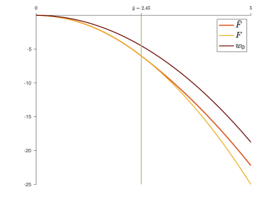
(a) $\delta=2$

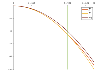
(b) $\delta=3/4$

Figure 1: the face-lifted utility $\bar{F}$

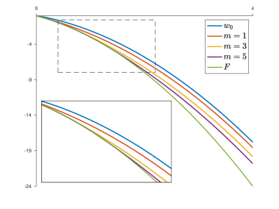
(a) $\delta=2$

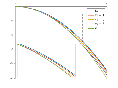
(b) $\delta=3/4$

Figure 2: the face-lifted utility $\bar{F}$ for different values of $m$

As discussed in Example 3.7, the positive power utility exhibits only a singular scenario when $\delta>1$. Consequently, we slightly modify the utility function by considering $F(y)=-y^{\gamma}-\gamma y$, for $y\geq 0$. It is important to note that since this function is injective, it corresponds to a specific utility $u$, which cannot be expressed analytically. However, this is unnecessary for our analysis; what is significant is that $F^{\star}(\delta F^{\prime}(0))=-(\gamma-1)(\delta-1)^{\frac{\gamma}{\gamma-1}}>0$ since this condition ensures that both scenarios in Proposition 3.5 are feasible. We proceed by illustrating the face-lifted utility $\bar{F}$ in the case when $\gamma=2$ as before, but for different values of $m$. The plot in Figure 2a highlights a continuous dependence between the value of $m$ and the value of $\bar{y}$, and therefore a continuous dependence between the average size of accidents and the length of the interval where termination is the preferred choice. Specifically, it is evident that, as the size of the potential losses reduces, the value of $\bar{y}$ also decreases, while the function $\bar{F}$ increases until converging to the accident-free reward $w_{0}$. A similar analysis can be carried out for $\delta<1$; however, for numerical convenience, we consider the standard positive power utility setting $F(y)=-y^{\gamma}-\gamma y$, for $y\geq 0$, where we set $\gamma=2$. The results are plotted in Figure 2b. Analogously to the case $\delta>1$, we can observe a correlation between the value $m$ and $\tilde{y}$. The only difference is that the latter is null only in the absence of accidents, that is, when $m=0$.

4 The first-best problem

In this section, we analyse the first-best contracting problem, which represents the benchmark situation without moral hazard. Indeed, in this case, the principal has all the bargaining power, in the sense that she actually chooses both the contract and the effort of the agent under the constraint that his utility is above the reservation utility:

$$V^{\rm P,FB}\coloneqq\sup_{\begin{subarray}{c}(\mathbf{C},\nu)\in\mathfrak{C}\times\mathcal{U}\\ J^{\text{$\rm A$}}(\mathbf{C},\nu)\geq u(R)\end{subarray}}J^{\rm P}(\mathbf{C},\nu)=\sup_{\begin{subarray}{c}(\mathbf{C},\nu)\in\mathfrak{C}\times\mathcal{U}\\ J^{\text{$\rm A$}}(\mathbf{C},\nu)\geq u(R)\end{subarray}}\bar{J}^{\rm P}(\mathbf{C},\nu).$$ (4.1)

Note that this equality directly follows from the analysis in Section 2.5 as $\mathfrak{C}=\mathfrak{C}^{0}$. To characterise the solution to this contracting problem, we introduce the notation $v^{\text{$\rm FB$}}(y)$ to represent the maximal reward obtained by the principal when maintaining the utility of the agent at the level $y\geq 0$. This function is referred to as the first-best value function, and it holds that $V^{\rm P,FB}=v^{\text{$\rm FB$}}(u(R)).$ By introducing a Lagrange multiplier $\lambda\leq 0$ associated to the participation constraint of the agent and applying the classical Karush–Kuhn–Tucker method, we can always rewrite the first-best value function, for any $y\geq 0$, as

$$v^{\text{$\rm FB$}}(y)=\inf_{\lambda\leq 0}\bigg{\{}\lambda y+\sup_{(\mathbf{C},\nu)\in\mathfrak{C}\times\mathcal{U}}\mathbb{E}^{\mathbb{P}^{\text{$\nu$}}}\bigg{[}\big{(}\mathrm{e}^{-\rho\tau}F(\zeta)-\lambda\mathrm{e}^{-r\tau}\zeta\big{)}\mathbf{1}_{\{\tau<\infty\}}+\int_{0}^{\tau}\Big{(}\rho\mathrm{e}^{-\rho s}\big{(}\alpha_{s}-\beta_{s}+F(\eta_{s})\big{)}-\lambda r\mathrm{e}^{-rs}\big{(}\eta_{s}-h(\alpha_{s},\beta_{s})\big{)}\Big{)}\mathrm{d}s\bigg{]}\bigg{\}}.$$

Clearly, the above expression can be expressed in a more compact form as follows:

$$v^{\text{$\rm FB$}}(y)=\inf_{\lambda\leq 0}\bigg{\{}\lambda y+\sup_{T\geq 0}\bigg{\{}-\mathrm{e}^{-\rho T}F^{\star}\big{(}\lambda\mathrm{e}^{\rho(1-\delta)T}\big{)}\mathbf{1}_{\{T<\infty\}}+\int_{0}^{T}\rho\mathrm{e}^{-\rho t}\big{(}G^{\star}-F^{\star}\big{)}\big{(}\delta\lambda\mathrm{e}^{\rho(1-\delta)t}\big{)}\mathrm{d}t\bigg{\}}\bigg{\}}\;\text{for any}\;y\geq 0,$$ (4.2)

where we have introduced $G^{\star}(p)\coloneqq\sup_{(a,b)\in U}\{a-b+ph(a,b)\},\;\text{for}\;p\in\mathbb{R}.$ Notice that this function is clearly non-decreasing and convex. In particular, $G^{\star}(p)\in[-m,\bar{a}-\varepsilon_{m}]$ for all $p\leq 0$.

In the subsequent analysis, the study of the first-best problem (4.1) is divided into two separate investigations depending on the ratio $\delta$. Namely, when $\delta=1$, the problem can be easily tackled with the aforementioned Karush–Kuhn–Tucker method, while this classical method is not successful to provide a complete characterisation of the first-best value function when $\delta\neq 1$. Nevertheless, under the additional condition $\gamma\delta>1$, we can identify the first-best value function as the unique viscosity solution of the following obstacle problem:

$$\min\big{\{}v^{\text{$\rm FB$}}(y)-\bar{F}(y),F^{\star}(\delta(v^{\text{$\rm FB$}})^{\prime}(y))-\delta y(v^{\text{$\rm FB$}})^{\prime}(y)+v^{\text{$\rm FB$}}(y)-\mathcal{J}^{\text{$\rm FB$}}\big{(}(v^{\text{$\rm FB$}})^{\prime}(y),(v^{\text{$\rm FB$}})^{\prime\prime}(y)\big{)}\big{\}}=0,\;y>0,\;v^{\text{$\rm FB$}}(0)=v^{\text{$\rm FB$}}_{0},$$ (4.3)

for the operator

$$\mathcal{J}^{\text{$\rm FB$}}(p,q)\coloneqq G^{\star}(\delta p)\mathbf{1}_{(-\infty,0]}(q)+\infty\mathbf{1}_{(0,\infty)}(q),\;\text{for}\;(p,q)\in\mathbb{R}^{2}.$$ (4.4)

Here, the initial value $v^{\text{$\rm FB$}}_{0}$ is given by the expression (4.2), that is,

$$v^{\text{$\rm FB$}}_{0}\coloneqq\inf_{\lambda\leq 0}\sup_{T\geq 0}\bigg{\{}-\mathrm{e}^{-\rho T}F^{\star}\big{(}\lambda\mathrm{e}^{\rho(1-\delta)T}\big{)}\mathbf{1}_{\{T<\infty\}}+\int_{0}^{T}\rho\mathrm{e}^{-\rho s}(G^{\star}-F^{\star})\big{(}\lambda\delta\mathrm{e}^{\rho(1-\delta)s}\big{)}\mathrm{d}s\bigg{\}}\in[0,\bar{a}-\varepsilon_{m}).$$ (4.5)

Remark 4.1.

1. Notice that the value $\bar{a}-\varepsilon_{m}$ is not attainable. Achieving this value would require choosing $\alpha^{\star}=\bar{a}$, $\beta^{\star}=\varepsilon_{m}$, $\tau^{\star}=\infty$ and $\pi^{\star}=0$, but the contract $(\tau^{\star},\pi^{\star},\xi)$ does not satisfy the participation constraint of the agent for any choice of the lump-sum payment $\xi$ which is $\mathcal{F}_{\infty}$-measurable.

2. We cannot further simplify the expression in (4.5) since the function $G^{\star}$ is not always non-negative. As a result, the concavity of the conjugate $F^{\star}$ is not sufficient to guarantee that the supremum is reached at $T=\infty$, as it is shown in the proof of [44, Theorem 3.1] for the problem without accidents.

Despite the apparent differences emphasised previously, we get analogous results to those in [44, Theorem 3.1]. Specifically, we can prove that when $\delta=1$, the first-best value function touches the barrier $\bar{F}$ and, when this occurs, the two functions coincide forever. Conversely, when $\delta>1$, it can be shown that either the two aforementioned functions coincide in a right-neighbourhood of the origin or they never touch. Unfortunately, in the case where $\delta<1$, we are unable to proceed with the analysis; it is possible only when $\gamma\delta\leq 1$, as we can demonstrate that the problem degenerates. In fact, analogously to [44, Theorem 3.1], it can be shown that the principal can achieve her maximal value $\bar{a}-\varepsilon_{m}$, motivating the agent to exert maximal effort continuously and promising him a substantial lump-sum payment at a large retirement time.

Theorem 4.2.

1. Let $\gamma\delta\leq 1$. Then $v^{\text{$\rm FB$}}=\bar{a}-\varepsilon_{m}$ on $[0,\infty)$ and an optimal contract does not exist.

2. Let $\delta=1$, and introduce $\lambda_{G}\coloneqq\inf\{\lambda\leq 0:G^{\star}(\lambda)\geq 0\}\in(-\infty,0)$.

   1. If $\lambda_{G}\geq F^{\prime}(0)$, then $v^{\text{$\rm FB$}}=F$ on $[0,\infty);$

   2. otherwise if $\lambda_{G}<F^{\prime}(0)$, we have that $v^{\text{$\rm FB$}}(y)=F(y)$ for any $y\geq y^{F^{\text{$\star$}}}\coloneqq(F^{\star})^{\prime}(\lambda_{G})>0$. Additionally, the first-best value function is continuously differentiable and, defining $y^{F^{\text{$\star$}},G^{\text{$\star$}}}\coloneqq(F^{\star})^{\prime}(\lambda_{G})-(G^{\star})^{\prime}(\lambda_{G})$, determined by

      $$v^{\text{$\rm FB$}}(y)=\begin{cases}\inf_{\lambda\leq 0}\big{\{}y\lambda-F^{\star}(\lambda)+G^{\star}(\lambda)\big{\}}\mathbf{1}_{[0,0\wedge y^{\text{$F$}^{\text{$\star$}}\text{$,$}\text{$G$}^{\text{$\star$}}})}(y)+\big{(}y\lambda_{G}-F^{\star}(\lambda_{G})\big{)}\mathbf{1}_{[0\wedge y^{\text{$F$}^{\text{$\star$}}\text{$,$}\text{$G$}^{\text{$\star$}}},y^{\text{$F$}^{\text{$\star$}}})}(y),\;y\in[0,y^{F^{\text{$\star$}}}),\\ F(y),\;y\in[y^{F^{\text{$\star$}}},\infty).\end{cases}$$

3. Let $\delta\neq 1$ and $\gamma\delta>1$. We have that the first-best value function $v^{\text{$\rm FB$}}$ is the unique continuous viscosity solution of Equation 4.3 in the class of functions $v$ such that $|v(y)-\bar{F}(y)|\leq C$ for any $y\geq 0$, for some $C>0$.

   1. Let $\delta>1$. If $v^{\text{$\rm FB$}}_{0}=0$, then there exists $\varepsilon>0$ such that $v^{\text{$\rm FB$}}=\bar{F}$ on $[0,\varepsilon]$. Moreover, it is true that $v^{\text{$\rm FB$}}=\bar{F}$ on $[0,\infty)$ if $m\leq F^{\star}(\delta F^{\prime}(0));$

   2. otherwise if $v^{\text{$\rm FB$}}_{0}>0$, and $\delta>1$, then it holds that $v^{\text{$\rm FB$}}>\bar{F}$ on $[0,\infty)$. Furthermore, it is twice continuously differentiable, and with $\lambda^{\star}_{0}\coloneqq(v^{\text{$\rm FB$}})^{\prime}(0)\in(-\infty,0)$ such that

      $$v^{\text{$\rm FB$}}=\big{(}v^{\text{$\rm FB$},\star}\big{)}^{\star},\;\text{\rm where}\;v^{\text{$\rm FB$},\star}(p)=-(-p)^{\frac{1}{1-\delta}}\Bigg{(}\frac{v^{\text{$\rm FB$}}_{0}}{(-\lambda^{\star}_{0})^{\frac{1}{1-\delta}}}-\frac{1}{{\delta-1}}\int_{p}^{\lambda^{\text{$\star$}}_{\text{$0$}}}\frac{F^{\star}(\delta x)-G^{\star}(\delta x)}{(-x)^{1+\frac{1}{1-\delta}}}\mathrm{d}x\Bigg{)},\;p\leq\lambda^{\star}_{0}.$$

   3. Let $\delta<1$, and assume that $\frac{\partial h}{\partial a}(0,b)>0$ for any $b\in B$ and $\frac{\partial h}{\partial b}(a,m)<0$ for any $a\in A$. We can define $y_{m}\coloneqq\inf\{y\geq 0:G^{\star}(\delta w_{0}^{\prime}(y))=-m\}\in(-\infty,0)$, recalling that $w_{0}$ represents the face-lifted reward in the problem without accidents as introduced in (3.6). If $v^{\text{$\rm FB$}}(y^{0})=\bar{F}(y^{0})$ for some $y^{0}\in[y_{m}\vee\tilde{y},\infty)$, then $v^{\text{$\rm FB$}}=\bar{F}$ on $[y^{0},\infty)$.

The proof of the first result follows; we show the remaining items in the subsequent sections and in Appendix B.

Proof of Theorem 4.2.$(i)$.

The fact that the first-best value function $v^{\text{$\rm FB$}}$ is constantly equal to $\bar{a}-\varepsilon_{m}$ on $[0,\infty)$ follows directly from Theorem 5.7.$(i)$. Furthermore, this value can only be achieved by selecting the effort $(\alpha^{\star},\beta^{\star})=(\bar{a},\varepsilon_{m})$ and the contract $\mathbf{C}^{\star}=(\tau^{\star},\pi^{\star},\xi^{\star})$ with $\tau^{\star}=\infty$ and $\pi^{\star}=0$. However, as highlighted in Remark 4.1.$(i)$, this contract fails to meet the participation constraint of the agent. ∎

Remark 4.3.

1. Definition 2.4 can be readily translated into the first-best setting. Specifically, we say that the first-contracting problem (4.1) exhibits a golden parachute if an optimal solution satisfies $\xi^{\star}>0$ on the event set $\{\tau^{\star}<\infty\}$. Based on Theorem 4.2.$(ii)$, we can conclude that when $\delta=1$ and $\lambda_{G}<F^{\prime}(0)$, a first-best golden parachute always exists, and it represents a termination scenario. In other words, the agent stops working at a finite time $($null if the reservation utility of the agent exceeds $y^{F^{\text{$\star$}}})$ leading to the termination of the contract, and the principal paying a positive lump-sum payment. The same holds if $\lambda_{G}\geq F^{\prime}(0)$ and the agent has a positive reservation utility. In this case, the termination time is always zero, signifying that the contract does not start, and the agent receives his reservation utility as payment.

2. Theorem 4.2.$(iii)$$(iii$-$1)$ directly implies analogous conclusions when $\delta>1$, $v^{\text{$\rm FB$}}_{0}=0$ and $m\leq F^{\star}(\delta F^{\prime}(0))$. In fact, if the reservation utility of the agent is positive, the first-best problem exhibits a golden parachute. However, since in this case the face-lifted function $\bar{F}$ is strictly above $F$, the contract does not terminate immediately. Instead, the agent does zero effort right from the beginning of the contract, he is immediately retired, and receives a continuous stream of payments. This scenario is never possible in the absence of accidents. In fact, according to [44, Theorem 3.1], there is no golden parachute whenever $\delta>1$. This is because the initial value $v^{\text{$\rm FB$}}_{0}$ is always positive when $m=0$, as the function $G^{\star}$ is non-negative.

3. The same result as in the case without accidents holds when $\delta>1$ and $v^{\text{$\rm FB$}}_{0}>0$. Theorem 4.2.$(iii)$$(iii$-$2)$ states that a first-best golden parachute does not exist since the first-best value function $v^{\text{$\rm FB$}}$ never touches its barrier $\bar{F}$ on $[0,\infty)$.

4. The case of $\delta<1$ and $\gamma\delta>1$ is the only one that we are unable to analyse in detail. Given the explicit form of the face-lifted utility $\bar{F}$ expressed in Proposition 3.10.$(ii)$, particularly the fact that it is only continuous, we expect that the first-best value function $v^{\text{$\rm FB$}}$ might not be smooth on the entire interval of definition $[0,\infty)$. Furthermore, we suspect that, similar to the accident-free framework, there exists a point from which $v^{\text{$\rm FB$}}$ and its barrier $\bar{F}$ coincide if $\frac{\partial h}{\partial a}(0,b)>0$ for any $b\in B$ and $\frac{\partial h}{\partial b}(a,m)<0$ for any $a\in A$. If this were to be confirmed, we could conclude that a first-best golden parachute exists whenever $v^{\text{$\rm FB$}}_{\text{$0$}}>0$, and this might also be a termination scenario, unlike the case with $m=0$ where the golden parachute always represents a retirement scenario. Conversely, if $v^{\text{$\rm FB$}}_{\text{$0$}}=0$, we could not automatically claim the existence of a golden parachute, we would need to pay attention to the interval of the non-negative half-line that we are considering. Note that the condition $\frac{\partial h}{\partial a}(0,b)>0$ for any $b\in B$ and $\frac{\partial h}{\partial b}(a,m)<0$ for any $a\in A$ is fundamental to ensure that the face-lifted utility $\bar{F}$ is a super-solution $($and hence a solution, considering that $G^{\star}\geq-m$ on the whole real line$)$ of Equation 4.3 from a certain point onwards. This is the same condition required in [44, Theorem 3.1] for $m=0$. In this case, it is proved that when the marginal cost of effort at zero is null, the first-best value function never touches the barrier $\bar{F}$, thereby ruling out the existence of a first-best golden parachute.

4.1 The Karush–Kuhn–Tucker method

Proof of Theorem 4.2.$(ii)$.

The first-best value function, as expressed in (4.2), can be further simplified when $\delta=1$:

$$v^{\text{$\rm FB$}}(y)=\inf_{\lambda\leq 0}\bigg{\{}\lambda y-F^{\star}(\lambda)+\sup_{T\geq 0}\big{\{}G^{\star}(\lambda)\big{(}1-\mathrm{e}^{-\rho T}\big{)}\big{\}}\bigg{\}}\;\text{for any}\;y\geq 0.$$

The optimisation with respect to the variable $T$ yields the following problem:

$$v^{\text{$\rm FB$}}(y)=\inf_{\lambda\leq 0}\Big{\{}\lambda y-F^{\star}(\lambda)+G^{\star}(\lambda)\mathbf{1}_{(\lambda_{\text{$G$}},0]}(\lambda)\Big{\}}.$$ (4.6)

If $\lambda_{G}\geq F^{\prime}(0)$, the optimisation with respect to $\lambda$ implies that $v^{\text{$\rm FB$}}(y)=\inf_{\lambda\leq 0}\big{\{}\lambda y-F^{\star}(\lambda)\big{\}}=F(y).$ This is because $y-(F^{\star})^{\prime}(\lambda)+(G^{\star})^{\prime}(\lambda)=y+(G^{\star})^{\prime}(\lambda)>0$ for any $y\in(\lambda_{G},0]$. We can deduce that $v^{\text{$\rm FB$}}=F$ on $[0,\infty)$.

On the other hand, we assume now that $\lambda_{G}<F^{\prime}(0)$. Considering the reformulation of the first-best problem as shown in (4.6), we describe the function $v^{\text{$\rm FB$}}$ by distinguishing three distinct cases depending on which interval of the non-negative half-line we are considering. To begin, let us suppose that $y\in(0,0\vee y^{F^{\text{$\star$}},G^{\text{$\star$}}})$. It is worth noting that this interval can be empty because $y^{F^{\text{$\star$}},G^{\text{$\star$}}}$ can be non-positive. If this is not the case, then we have that $y-(F^{\star})^{\prime}(\lambda_{G})+(G^{\star})^{\prime}(\lambda_{G})<0$, and

$$v^{\text{$\rm FB$}}(y)=\inf_{\lambda\in(\lambda_{\text{$G$}},0)}\big{\{}\lambda y-F^{\star}(\lambda)+G^{\star}(\lambda)\big{\}}=\inf_{\lambda\leq 0}\big{\{}\lambda y-F^{\star}(\lambda)+G^{\star}(\lambda)\big{\}}.$$

We then consider the case where $y\in[0\vee y^{F^{\text{$\star$}},G^{\text{$\star$}}},y^{F^{\text{$\star$}}})$. It holds that $y-(F^{\star})^{\prime}(\lambda_{G})+(G^{\star})^{\prime}(\lambda_{G})\geq 0$ and $y-(F^{\star})^{\prime}(\lambda_{G})<0$ because of the definition of the two points $y^{F^{\text{$\star$}},G^{\text{$\star$}}}$ and $y^{F^{\text{$\star$}}}$. Hence, $v^{\text{$\rm FB$}}$ is a linear function of the following form $v^{\text{$\rm FB$}}(y)=y\lambda_{G}-F^{\star}(\lambda_{G}).$ Lastly, when we have $y\in[y^{F^{\text{$\star$}}},\infty)$, it follows that $y-(F^{\star})^{\prime}(\lambda_{G})\geq 0$. As a consequence,

$$v^{\text{$\rm FB$}}(y)=\inf_{\lambda\leq\lambda_{G}}\big{\{}\lambda y-F^{\star}(\lambda)\big{\}}=\inf_{\lambda\leq 0}\big{\{}\lambda y-F^{\star}(\lambda)\big{\}}=F(y).$$

Reviewing the computations done so far, we can deduce that $v^{\text{$\rm FB$}}>F$ on $[0,y^{F^{\text{$\star$}}})$. Moreover, the first-best value function $v^{\text{$\rm FB$}}$ is not only continuous but also continuously differentiable since

$$(v^{\text{$\rm FB$}})^{\prime}_{-}(y^{F^{\text{$\star$}},G^{\text{$\star$}}})\mathbf{1}_{\{y^{\text{$F$}^{\text{$\star$}}\text{$,$}\text{$G$}^{\text{$\star$}}}>0\}}=(v^{\text{$\rm FB$}})^{\prime}_{+}(y^{F^{\text{$\star$}},G^{\text{$\star$}}})\mathbf{1}_{\{y^{\text{$F$}^{\text{$\star$}}\text{$,$}\text{$G$}^{\text{$\star$}}}>0\}}=\lambda_{G}=(v^{\text{$\rm FB$}})^{\prime}_{-}(y^{\text{$F^{\star}$}})=(v^{\text{$\rm FB$}})^{\prime}_{+}(y^{F^{\text{$\star$}}}).$$

∎

Example 4.4.

In the specific framework of the positive power utility described in Example 3.4 with $\delta=1$, we have $\bar{F}(y)=F(y)=-y^{\gamma},\;\text{\rm for}\;y\geq 0.$ Additionally, let us set some $\bar{a}$, $\varepsilon_{m}$ and $m$ such that $\bar{a}>0$ and $0<\varepsilon_{m}<m$, and consider the following cost function:

$$h(a,b)\coloneqq h_{a}(a)+h_{b}(b)\coloneqq\frac{a^{2}}{2}+\bigg{(}\frac{1}{b}-\frac{1}{m}\bigg{)},\;\text{\rm where}\;(a,b)\in A\times B\coloneqq[0,\bar{a}]\times[\varepsilon_{m},m].$$

The decision to consider a separate cost in the two tasks of applying effort and reducing accident risk is solely for purely analytical reasons, as it significantly simplifies the calculations, allowing us to explicitly characterise the convex dual

$$G^{\star}(p)=G^{\star}_{a}(p)+G^{\star}_{b}(p)\coloneqq\sup_{a\in[0,\bar{a}]}\{a+ph_{a}(a)\}+\sup_{b\in[\varepsilon_{\text{$m$}},m]}\{-b+ph_{b}(b)\}\;\text{\rm for any}\;p\in\mathbb{R}.$$

Under the present specification, we have that

$$G^{\star}_{a}(p) =-\frac{1}{2p}\mathbf{1}_{\{p\leq-1/\bar{a}\}}+\bar{a}\Big{(}1+\frac{\bar{a}}{2}p\Big{)}\mathbf{1}_{\{p>-1/\bar{a}\}},$$

$$G^{\star}_{b}(p) =-m\mathbf{1}_{\{p\leq-m^{\text{$2$}}\}}-\big{(}2m-(-p)^{\frac{1}{2}}\big{)}\frac{(-p)^{\frac{1}{2}}}{m}\mathbf{1}_{\{-m^{\text{$2$}}<p<-\varepsilon_{\text{$m$}}^{\text{$2$}}\}}-\bigg{(}\varepsilon_{m}+\bigg{(}\frac{1}{m}-\frac{1}{\varepsilon_{m}}\bigg{)}p\bigg{)}\mathbf{1}_{\{p\geq-\varepsilon_{m}^{\text{$2$}}\}},\;\text{\rm for}\;p\in\mathbb{R}.$$

Given this specific choice of the utility function $F$, particularly noting that $F^{\prime}(0)=0$, we fall into the second scenario of Theorem 4.2.$(ii)$. Consequently, the first-best value function is not identically equal to its barrier $F$, but we are unable to provide explicit formulas since $y^{{F}^{\text{$\star$}}{,}{G}^{\text{$\star$}}}$ and $y^{{F}^{\text{$\star$}}}$ cannot be computed analytically. Setting $\gamma=2$, $\bar{a}=0.6$, $\varepsilon_{m}=0.1$ and $m=0.3$, we plot our numerical results below. Specifically, we observe that $y^{{F}^{\text{$\star$}}{,}{G}^{\text{$\star$}}}$ is positive, and therefore, the function $v^{\text{$\rm FB$}}$ is a strictly concave solution to the ODE that characterises the obstacle problem (4.3) within the interval $[0,y^{{F}^{\text{$\star$}}{,}{G}^{\text{$\star$}}})$, is affine on $[y^{{F}^{\text{$\star$}}{,}{G}^{\text{$\star$}}},y^{{F}^{\text{$\star$}}}]$, and then coincides with $F$ on $(y^{{F}^{\text{$\star$}}},\infty)$. It is worth noting that contrary to the results in [44], the function is not strictly concave on the whole domain of definition. Additionally, it is only continuously differentiable, as the gluing of the functions $\inf_{\lambda\leq 0}\{y\lambda-F^{\star}(\lambda)+G^{\star}(\lambda)\}$, for $y\in[0,y^{\text{$F$}^{\text{$\star$}}\text{$,$}\text{$G$}^{\text{$\star$}}})$, $y\lambda_{G}-F^{\star}(\lambda_{G})$, for $y\in[y^{\text{$F$}^{\text{$\star$}}\text{$,$}\text{$G$}^{\text{$\star$}}},y^{\text{$F$}^{\text{$\star$}}})$, and $F(y)$, for $y\in(y^{\text{$F$}^{\text{$\star$}}},\infty)$, is only continuously differentiable. These differences arise from the fact that $G^{\star}$ can be negative in our framework with accidents.

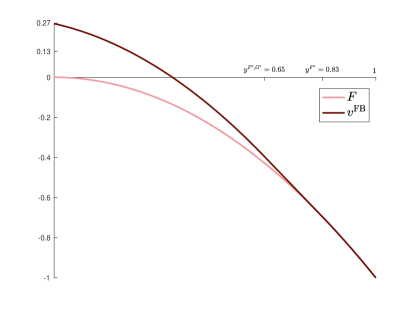
Figure 3: the first-best value function $v^{\text{$\rm FB$}}$ and its barrier $F$

4.2 HJB approach

In order to solve the first-best version (4.1) of the contracting problem when $\delta\neq 1$ and $\gamma\delta>1$, we follow the general approach developed by [33, Section 4]. More precisely, we show that there is no loss of generality when the principal solves her first-best problem in maximising over the set $\mathcal{V}^{\text{$\rm FB$}}(Y^{{\rm A}}_{0})$, which we introduce later in Theorem 4.6, as opposed to optimising over $\mathfrak{C}\times\mathcal{U}$ such that the participation constraint is satisfied. This reduction simplifies the first-best problem to a standard stochastic control problem, making it more tractable.

To begin, let us fix a stopping time $\tau$, an $\mathbb{F}$-predictable non-negative process $\pi$ and a control $\nu\in\mathcal{U}$. For a constant $Y^{{\rm A}}_{0}\in\mathbb{R}$, an $\mathbb{R}$-valued $\mathbb{F}$-predictable process $Z^{{\rm A}}$ and an $\mathbb{R}$-valued $\widetilde{\mathcal{P}}(\mathbb{F})$-measurable function $U^{{\rm A}}$, we introduce the process $Y^{\text{$\rm FB$},{Y}^{\text{$\rm A$}}_{\text{$0$}}{,}{Z}^{\text{$\rm A$}}{,}{U}^{\text{$\rm A$}},\pi}$ defined by the following SDE, for $t\geq 0$:

$$Y^{\text{$\rm FB$},{Y}^{\text{$\rm A$}}_{\text{$0$}}{,}{Z}^{\text{$\rm A$}}{,}{U}^{\text{$\rm A$}}{,}{\pi}}_{t}=Y^{{\rm A}}_{0}+\int_{0}^{t}r\big{(}Y^{\text{$\rm FB$},{Y}^{\text{$\rm A$}}_{\text{$0$}}{,}{Z}^{\text{$\rm A$}}{,}{U}^{\text{$\rm A$}}{,}{\pi}}_{s}-u(\pi_{s})+h(\nu_{s})\big{)}\mathrm{d}s+r\sigma\int_{0}^{t}Z^{{\rm A}}_{s}\mathrm{d}W^{\nu}_{s}+r\int_{0}^{t}\int_{\mathbb{R}^{\text{$+$}}}U^{{\rm A}}_{s}(\ell)\tilde{\mu}^{{J}^{\text{$\nu$}}}(\mathrm{d}s,\mathrm{d}\ell),$$ (4.7)

where $\tilde{\mu}^{{J}^{\text{$\nu$}}}$ denotes the $(\mathbb{F},\mathbb{P}^{\nu})$-compensated random measure $\mu^{J}-\mu^{J^{\text{$\nu$}},p}$. Then, we introduce the set $\mathcal{V}^{\text{$\rm FB$}}_{\tau}$ as the collection of all $Z^{{\rm A}}$ and $U^{{\rm A}}$ defined as previously, satisfying in addition the following integrability conditions

$$\sup_{\nu\in\mathcal{U}}\mathbb{E}^{\mathbb{P}^{\text{$\nu$}}}\bigg{[}\sup_{t\geq 0}\Big{|}\mathrm{e}^{-\kappa(t\wedge\tau)}Y^{\text{$\rm FB$},{Y}^{\text{$\rm A$}}_{\text{$0$}}{,}{Z}^{\text{$\rm A$}}{,}{U}^{\text{$\rm A$}}{,}{\pi}}_{t\wedge\tau}\Big{|}^{p}\bigg{]}<\infty,$$

$$\sup_{\nu\in\mathcal{U}}\mathbb{E}^{\mathbb{P}^{\text{$\nu$}}}\Bigg{[}\bigg{(}\int_{0}^{\tau}\mathrm{e}^{-2\kappa s}|Z^{{\rm A}}_{s}|^{2}\mathrm{d}s\bigg{)}^{\frac{p}{2}}\Bigg{]}<\infty,\;\text{and}\;\sup_{\nu\in\mathcal{U}}\mathbb{E}^{\mathbb{P}^{\text{$\nu$}}}\Bigg{[}\bigg{(}\int_{0}^{\tau}\int_{\mathbb{R}^{\text{$+$}}}\mathrm{e}^{-2\kappa s}|U^{{\rm A}}_{s}(\ell)|^{2}\Phi(\mathrm{d}\ell)\mathrm{d}s\bigg{)}^{\frac{p}{2}}\Bigg{]}<\infty,$$

for some $\kappa\in(0,r)$, $p>2$.

Remark 4.5.

Note that based on Øksendal and Sulem [39, Theorem 1.19], the Lipschitz-continuity in the $y$-variable of the drift implies that the SDE (4.7) has a pathwise unique solution up to the random time $\tau$. Furthermore, we always consider a càdlàg $\mathbb{P}$-modification of the process $Y^{\text{$\rm FB$},{Y}^{\text{$\rm A$}}_{\text{$0$}}{,}{Z}^{\text{$\rm A$}}{,}{U}^{\text{$\rm A$}}{,}{\pi}}$.

For any $Y^{{\rm A}}_{0}\in\mathbb{R}$, we define the set $\mathcal{V}^{\text{$\rm FB$}}(Y^{{\rm A}}_{0})$ as the collection of all quintuples $(\tau,\pi,\nu,Z^{{\rm A}},U^{{\rm A}})$, where $\tau$ is an $\mathbb{F}$–stopping time, $\pi$ is an $\mathbb{F}$-predictable non-negative process, and $(Z^{{\rm A}},U^{{\rm A}})\in\mathcal{V}^{\text{$\rm FB$}}_{\tau}$, that verify that

$$\text{the contract}\;\mathbf{C}\coloneqq\big{(}\tau,\pi,u^{-1}\big{(}Y^{\text{$\rm FB$},{Y}^{\text{$\rm A$}}_{\text{$0$}}{,}{Z}^{\text{$\rm A$}}{,}{U}^{\text{$\rm A$}}{,}{\pi}}_{\tau}\big{)}\big{)}\;\text{satisfies the integrability conditions \eqref{eq:integrabilityCondition}}.$$

Theorem 4.6.

It holds that

$$V^{\rm P,FB}=\sup_{(\tau,\pi,\nu,Z^{\text{$\rm A$}},U^{\text{$\rm A$}})\in\mathcal{V}^{\text{$\rm FB$}}(u(R))}\mathbb{E}^{\mathbb{P}^{\text{$\nu$}}}\bigg{[}\mathrm{e}^{-\rho\tau}\bar{F}\big{(}Y^{\text{$\rm FB$},{Y}^{\text{$\rm A$}}_{\text{$0$}}{,}{Z}^{\text{$\rm A$}}{,}{U}^{\text{$\rm A$}}{,}{\pi}}_{\tau}\big{)}\mathbf{1}_{\{\tau<\infty\}}+\int_{0}^{\tau}\rho\mathrm{e}^{-\rho s}(\alpha_{s}-\beta_{s}-\pi_{s})\mathrm{d}s\bigg{]}.$$

Proof.

The proof follows by simply adapting the arguments in Theorem 5.2 taking into account that, for any contract $\mathbf{C}=(\tau,\pi,\xi)\in\mathfrak{C}$ and any control $\nu\in\mathcal{U}$, the process defined as

$$M^{\text{$\rm A$}\text{$,$}\text{$\rm FB$}}_{t}(\mathbf{C},\nu)\coloneqq V^{\text{$\rm A$}\text{$,$}\text{$\rm FB$}}_{t\wedge\tau}(\mathbf{C},\nu)\mathrm{e}^{-r(t\wedge\tau)}+\int_{0}^{t\wedge\tau}r\mathrm{e}^{-rs}(u(\pi_{s})-h(\nu_{s}))\mathrm{d}s,\;\text{for}\;t\geq 0,$$ (4.8)

is a $\mathbb{P}^{\nu}$–uniformly integrable $(\mathbb{F},\mathbb{P}^{{\nu}})$-martingale (see for instance [27, Theorem I.1.42]). Here,

$$V^{\text{$\rm A$}\text{$,$}\text{$\rm FB$}}_{t}(\mathbf{C},\nu)\coloneqq\mathbb{E}^{\mathbb{P}^{\text{$\nu$}}}_{t}\bigg{[}\mathrm{e}^{-r(\tau-t)}u(\xi)\mathbf{1}_{\{\tau<\infty\}}+\int_{t}^{\tau}r\mathrm{e}^{-r(s-t)}(u(\pi_{s})-h(\nu_{s}))\mathrm{d}s\bigg{]},\;\text{for}\;t\in[0,\tau].$$

∎

Remark 4.7.

From the representation provided in (4.2) of the first-best value function $v^{\text{$\rm FB$}}$, we immediately infer that it is non-increasing, given that the Lagrange multipliers $\lambda$ take values in the non-positive half-line. This implies that the reward of agent is exactly given by his participation constraint $u(R)$. Consequently, if an optimal contract $\mathbf{C}^{\star}$ exists for the first-best contracting problem, it has the following form

$$\mathbf{C}^{\star}\coloneqq\big{(}\tau^{\star},\pi^{\star},u^{-1}\big{(}Y^{\text{$\rm FB$},{Y}^{\text{$\rm A$}}_{\text{$0$}}{,}{Z}^{\text{$\rm A$}}{,}{U}^{\text{$\rm A$}}{,}{\pi^{\text{$\star$}}}}_{\tau}\big{)}\big{)},$$

where $\tau^{\star}$ is an $\mathbb{F}$–stopping time, $\pi^{\star}$ is an $\mathbb{F}$-predictable non-negative process and $(Z^{{\rm A}},U^{{\rm A}})\in\mathcal{V}^{\text{$\rm FB$}}_{\tau^{\text{$\star$}}}$.

Theorem 4.6 reduces the complexity of the problem. This reduction simplifies the problem by associating the first-best value function $v^{\text{$\rm FB$}}$ with the corresponding Hamilton–Jacobi–Bellman equation, as presented in (4.3), following the classical reasoning in control theory. Our next objective is to show that the value function $v^{\text{$\rm FB$}}$ is the unique viscosity solution of the aforementioned equation in the class of functions that behave like $\bar{F}$ at infinity. Before verifying this statement, it is necessary to prove that our value function exhibits the desired growth.

Lemma 4.8.

If $\delta\neq 1$ and $\gamma\delta>1$, then there exists some $C>0$ such that $|v^{\text{$\rm FB$}}(y)-\bar{F}(y)|\leq C$ for any $y\geq 0$.

Proof.

The definition of the first-best problem straightforwardly implies that $v^{\text{$\rm FB$}}-\bar{F}\geq-C$ on $[0,\infty)$, where $C>0$. To prove the reverse bound, we first introduce the function

$$\iota(y)\coloneqq\inf_{\lambda\leq 0}\bigg{\{}\lambda y-\int_{0}^{\infty}\rho\mathrm{e}^{-\rho s}F^{\star}\big{(}\lambda\delta\mathrm{e}^{\rho(1-\delta)s}\big{)}\mathrm{d}s\bigg{\}},\;\text{for}\;y\geq 0.$$

For any $y\geq 0$, we note that

$$v^{\text{$\rm FB$}}(y) =\inf_{\lambda\leq 0}\bigg{\{}\lambda y+\sup_{T\geq 0}\bigg{\{}-\mathrm{e}^{-\rho T}F^{\star}\big{(}\lambda\mathrm{e}^{\rho(1-\delta)T}\big{)}\mathbf{1}_{\{T<\infty\}}+\int_{0}^{T}\rho\mathrm{e}^{-\rho s}\big{(}G^{\star}-F^{\star}\big{)}\big{(}\lambda\delta\mathrm{e}^{\rho(1-\delta)s}\big{)}\mathrm{d}s\bigg{\}}\bigg{\}}$$

$$\leq\inf_{\lambda\leq 0}\bigg{\{}\lambda y+\sup_{T\geq 0}\bigg{\{}-\mathrm{e}^{-\rho T}F^{\star}\big{(}\lambda e^{\rho(1-\delta)T}\big{)}\mathbf{1}_{\{T<\infty\}}-\int_{0}^{T}\rho\mathrm{e}^{-\rho s}F^{\star}\big{(}\lambda\delta\mathrm{e}^{\rho(1-\delta)s}\big{)}\mathrm{d}s\bigg{\}}+\bar{a}-\varepsilon_{m}=\iota(y)+\bar{a}-\varepsilon_{m},$$

where the second inequality is a consequence of the definition of $G^{\star}$, while the last equality follows from the concavity of $F^{\star}$. Consequently, it is sufficient to verify that there exists a constant $C>0$ such that

$$\iota(y)-\bar{F}(y)\leq C\;\text{for any}\;y\geq 0.$$ (4.9)

We can divide the proof into three distinct parts, depending on the specific case under consideration and the corresponding face-lifted utility $\bar{F}$. In the scenario where $\delta>1$ and $m\leq-F^{\star}(\delta F^{\prime}(0))$, the function $\bar{F}$ is given in terms of its concave conjugate $w^{\star}$ introduced in (A.3). Based on its description, we can deduce that

$$w^{\star}(p)\leq m+\frac{(-p)^{\frac{1}{1-\delta}}}{\delta-1}\int_{p}^{0}\frac{F^{\star}(\delta x)}{(-x)^{1+\frac{1}{1-\delta}}}\mathrm{d}x=m+\int_{0}^{\infty}\rho\mathrm{e}^{-\rho t}F^{\star}\big{(}\delta p\mathrm{e}^{\rho(1-\delta)t}\big{)}\mathrm{d}t\;\text{for any}\;p\leq\frac{(F^{\star})^{-1}(-m)}{\delta}.$$

In the first inequality, we have used the fact that $F^{\star}(\delta x)+m\geq 0$ for any $x\in[f_{\delta m},0]$ followed by the change of variables $x\longmapsto p\mathrm{e}^{\rho(1-\delta)t}$. From the previous inequality, it becomes evident that $\iota(y)-\bar{F}(y)\leq m$ for all $y\geq 0$. We can conclude that the inequality in (4.9) is satisfied.

When the jumps become larger, specifically in the case of $\delta>1$ and $m>-F^{\star}(\delta F^{\prime}(0))$, we have that $\bar{F}=F$ on $[0,\bar{y}]$. As the function $\iota$ is upper–semi-continuous since it is an infimum of an arbitrary family of continuous functions, we can deduce the existence of a constant $C>0$ such that $(\iota-F)(y)\leq C$ for any $y\in[0,\bar{y}]$. Nonetheless, we still need to provide a similar bound on $(F^{\prime}(\bar{y}),\infty)$, where $\bar{F}$ is described by the concave conjugate of $w^{\star}_{\bar{y}}$ as given in (A.8). Its explicit formula is as follows, for any $p\in(-\infty,F^{\prime}(\bar{y}))$:

$$w^{\star}_{\bar{y}}(p) =\frac{(-p)^{\frac{1}{1-\delta}}}{\delta-1}\int_{p}^{F^{\prime}(\bar{y})}\frac{F^{\star}(\delta x)+m}{(-x)^{1+\frac{1}{1-\delta}}}\mathrm{d}x+F^{\star}(F^{\prime}(\bar{y}))\left(\frac{p}{F^{\prime}(\bar{y})}\right)^{\frac{1}{1-\delta}}$$

$$\leq\frac{(-p)^{\frac{1}{1-\delta}}}{\delta-1}\int_{p}^{F^{\prime}(\bar{y})}\frac{F^{\star}(\delta x)+m}{(-x)^{1+\frac{1}{1-\delta}}}\mathrm{d}x$$

$$=\frac{(-p)^{\frac{1}{1-\delta}}}{\delta-1}\int_{p}^{0}\frac{F^{\star}(\delta x)+m}{(-x)^{1+\frac{1}{1-\delta}}}\mathrm{d}x-\frac{(-p)^{\frac{1}{1-\delta}}}{\delta-1}\int_{F^{\prime}(\bar{y})}^{0}\frac{F^{\star}(\delta x)+m}{(-x)^{1+\frac{1}{1-\delta}}}\mathrm{d}x\leq C+\frac{(-p)^{\frac{1}{1-\delta}}}{\delta-1}\int_{p}^{0}\frac{F^{\star}(\delta x)+m}{(-x)^{1+\frac{1}{1-\delta}}}\mathrm{d}x,$$

for some $C>0$. This allows us to conclude by applying the same change of variables as we did previously.

Lastly, we examine the scenario where $\delta<1$ and $\gamma\delta>1$. It is straightforward to prove that the inequality in (4.9) is satisfied on the interval $[0,\tilde{y}]$. Additionally, for $y\in(\tilde{y},\infty)$, it holds that $\iota(y)=w_{0}(y)=\bar{F}(y)$, where the function $w_{0}$ is introduced in (3.6). This concludes the proof. ∎

Proof of Theorem 4.2.$(iii)$.

First, it is important to note that the operator $\mathcal{J}^{\text{$\rm FB$}}$ introduced in (4.4) is Lipschitz-continuous and non-decreasing with respect to its second variable. These properties are sufficient to say that the same techniques presented in [44, Lemma B.1] work in our setting to prove a comparison theorem for the Hamilton–Jacobi–Bellman equation (4.3) in the class of functions $v$ verifying $|v(y)-\bar{F}(y)|\leq C$, $y\geq 0$, for some $C>0$. Furthermore, standard arguments from viscosity solution theory show that $v^{\text{$\rm FB$}}$ is a discontinuous viscosity solution of Equation 4.3 (the approach is similar to the one in Proposition A.11). Consequently, Lemma 4.8 allows to apply the aforementioned comparison theorem to the function $v^{\text{$\rm FB$}}$, leading to the conclusion that $v^{\text{$\rm FB$}}$ is the unique viscosity solution, in that class of functions, and it is continuous. ∎

Proof of Theorem 4.2.$(iii)$$(iii$-$3)$.

By assumption, there exists some $y^{0}\in[y_{m}\vee\tilde{y},\infty)$ such that $v^{\text{$\rm FB$}}(y^{0})=\bar{F}(y^{0})$. Since $y^{0}\geq\tilde{y}$, it follows that $\bar{F}(y)=w_{0}(y)-m$ for any $y\in[y^{0},\infty)$ due to Proposition 3.10.$(ii)$. Additionally, on this interval, $\bar{F}$ solves Equation 4.3 because the fact that $w_{0}$ is a decreasing function implies that $G^{\star}(\delta w_{0}^{\prime}(y))=-m$ for any $y\in[y^{0},\infty)$. Therefore, the comparison theorem mentioned in the proof of Theorem 4.2.$(iii)$ allows us to conclude. ∎

5 Reduction of the second-best contracting problem

This section focuses on reducing the Stackelberg game (2.8) of the principal to a standard mixed control–stopping stochastic problem, following the approach outlined in [47], which was further developed in [19]. This reduction is possible by introducing the continuation utility of the agent as an additional state variable, and then identifying a specific class of contracts $\mathbf{C}$ that reveal the optimal response $\nu^{\star}(\mathbf{C})$ of the agent, while ensuring no loss of generality. Before exploring further into this approach, it is essential to note that the Hamiltonian associated to the problem of the agent is defined as

$$H^{\rm A}(z^{\text{$\rm A$}},u^{\text{$\rm A$}})\coloneqq\sup_{(a,b)\in U}h^{\rm A}(z^{\text{$\rm A$}},u^{\text{$\rm A$}},a,b)\coloneqq\sup_{(a,b)\in U}\bigg{\{}az^{\text{$\rm A$}}-\frac{m-b}{m}\int_{\mathbb{R}_{+}}u^{\text{$\rm A$}}(\ell)\Phi(\mathrm{d}\ell)-h(a,b)\bigg{\}},\;\text{for}\;(z^{\text{$\rm A$}},u^{\text{$\rm A$}})\in\mathbb{R}\times\mathcal{B}_{\mathbb{R}}.$$ (5.1)

Let us introduce an $\mathbb{R}$-valued $\mathbb{F}$-predictable process $Z^{\rm A}$ and an $\mathbb{R}$-valued $\widetilde{\mathcal{P}}(\mathbb{F})$-measurable function $U^{\rm A}$. For any given $\mathbb{F}$–stopping time $\tau$, we define the set $\mathcal{U}^{\star}_{\tau}(Z^{{\rm A}},U^{{\rm A}})$ as the collection of efforts $\nu=(\alpha,\beta)\in\mathcal{U}$ such that

$$(\alpha_{t},\beta_{t})\in\operatorname*{arg\,max}_{(a,b)\in U}\big{\{}h^{\rm A}(Z^{\rm A}_{t},U^{\rm A}_{t},a,b)\big{\}},\;\mathrm{d}t\otimes\mathrm{d}\mathbb{P}\text{--a.e.}\;\text{on}\;\llbracket 0,\tau\rrbracket.$$ (5.2)

We also need to introduce a family of processes that will be used to reformulate the admissible lump-sum payments at terminal time received by the agent. Let us fix a constant $Y^{\rm A}_{0}\in\mathbb{R}$ along with a non-negative $\mathbb{F}$-predictable process $\pi$. We define the process $Y^{Y^{\text{$\rm A$}}_{\text{$0$}},Z^{\text{$\rm A$}},U^{\text{$\rm A$}},\pi}$ as the solution of the following SDE, for $t\geq 0$:

$$Y^{Y^{\text{$\rm A$}}_{\text{$0$}},Z^{\text{$\rm A$}},U^{\text{$\rm A$}},\pi}_{t}=Y^{\rm A}_{0}+\int_{0}^{t}r\big{(}Y^{Y^{\text{$\rm A$}}_{\text{$0$}},Z^{\text{$\rm A$}},U^{\text{$\rm A$}},\pi}_{s}-u(\pi_{s})-H^{\rm A}(Z^{\rm A}_{s},U^{\rm A}_{s})\big{)}\mathrm{d}s+r\sigma\int_{0}^{t}Z^{\rm A}_{s}\mathrm{d}W_{s}+r\int_{0}^{t}\int_{\mathbb{R}}U^{\rm A}_{s}(\ell)\tilde{\mu}^{{J}}(\mathrm{d}s,\mathrm{d}\ell).$$ (5.3)

Then, we introduce the set $\mathcal{V}^{\text{$\rm A$}}_{\tau}$ as the collection of all $\mathbb{R}$-valued, $\mathbb{F}$-predictable processes $Z^{\rm A}$ and $\mathbb{R}$-valued $\widetilde{\mathcal{P}}(\mathbb{F})$-measurable functions $U^{\rm A}$ such that the supremum (5.2) in the definition of $H^{\rm A}(Z_{t}^{{\rm A}},U_{t}^{{\rm A}})$ is attained. More precisely, we require that the set $\mathcal{U}^{\star}_{\tau}(Z^{{\rm A}},U^{{\rm A}})$ is not empty. Additionally, the following integrability conditions need to be satisfied

$$\sup_{\nu\in\mathcal{U}}\mathbb{E}^{\mathbb{P}^{\text{$\nu$}}}\bigg{[}\sup_{t\geq 0}\Big{|}\mathrm{e}^{-\kappa(t\wedge\tau)}Y^{Y^{\text{$\rm A$}}_{\text{$0$}},Z^{\text{$\rm A$}},U^{\text{$\rm A$}},\pi}_{t\wedge\tau}\Big{|}^{p}\bigg{]}<\infty,$$ (5.4)

$$\sup_{\nu\in\mathcal{U}}\mathbb{E}^{\mathbb{P}^{\text{$\nu$}}}\Bigg{[}\bigg{(}\int_{0}^{\tau}\mathrm{e}^{-2\kappa s}|Z^{\rm A}_{s}|^{2}\mathrm{d}s\bigg{)}^{\frac{p}{2}}\Bigg{]}<\infty,\;\text{and}\;\sup_{\nu\in\mathcal{U}}\mathbb{E}^{\mathbb{P}^{\text{$\nu$}}}\Bigg{[}\bigg{(}\int_{0}^{\tau}\int_{\mathbb{R}_{\text{$+$}}}\mathrm{e}^{-2\kappa s}|U^{\rm A}_{s}(\ell)|^{2}\Phi(\mathrm{d}\ell)\mathrm{d}s\bigg{)}^{\frac{p}{2}}\Bigg{]}<\infty,$$ (5.5)

for some $\kappa\in(0,r)$ and $p>2\vee\gamma$.

Remark 5.1.

1. As pointed out in Remark 4.5, the previous SDE admits a unique strong solution $Y^{Y^{\text{$\rm A$}}_{\text{$0$}},Z^{\text{$\rm A$}},U^{\text{$\rm A$}},\pi}$. We will prove that the process $Y^{Y^{\text{$\rm A$}}_{\text{$0$}},Z^{\text{$\rm A$}},U^{\text{$\rm A$}},\pi}$ represents the continuation utility of the agent given the contract $\mathbf{C}=(\tau,\pi,\xi)$, where $\xi=\xi^{Y^{\text{$\rm A$}}_{\text{$0$}},Z^{\text{$\rm A$}},U^{\text{$\rm A$}},\pi}\coloneqq u^{-1}\big{(}Y^{Y^{\text{$\rm A$}}_{\text{$0$}},Z^{\text{$\rm A$}},U^{\text{$\rm A$}},\pi}_{\tau}\big{)}$. In particular, $Y^{Y^{\text{$\rm A$}}_{\text{$0$}},Z^{\text{$\rm A$}},U^{\text{$\rm A$}},\pi}_{0}=V^{\rm A}(\mathbf{C})$.

2. We highlight the fact that the non-negativity condition imposed on both the utility function $u$ and the cost function $h$ is translated into a non-negativity constraint of the continuation utility of the agent, namely $Y^{Y^{\text{$\rm A$}}_{\text{$0$}},Z^{\text{$\rm A$}},U^{\text{$\rm A$}},\pi}_{t\wedge\tau}\geq 0$ for any $t\geq 0$, $\mathbb{P}$–a.s. This is just a consequence of a comparison theorem for BSDEs $($see for instance Papapantoleon, Possamaï, and Saplaouras [41, Theorem 3.25]$)$. Additionally, the limited liability constraint implies that

   $$Y^{Y^{\text{$\rm A$}}_{\text{$0$}},Z^{\text{$\rm A$}},U^{\text{$\rm A$}},\pi}_{t-}+r\int_{\mathbb{R}}U^{\rm A}_{t}(\ell)\Phi(\mathrm{d}\ell)\geq 0,\;\mathrm{d}t\otimes\mathrm{d}\mathbb{P}\text{\rm--a.e.}\;\text{\rm on}\;\llbracket 0,\tau\rrbracket.$$

Considering the previous discussion, we define the set $\mathcal{V}^{\text{$\rm S$}}(Y^{\rm A}_{0})$ as the collection all quadruples $(\tau,\pi,Z^{\rm A},U^{\rm A})$ verifying that $\tau$ is an $\mathbb{F}$–stopping time, $\pi$ is an $\mathbb{F}$-predictable non-negative process, and $(Z^{\rm A},U^{\rm A})\in\mathcal{V}_{\tau}^{\text{$\rm A$}}$. Additionally, the contract $(\tau,\pi,u^{-1}(Y^{Y^{\text{$\rm A$}}_{\text{$0$}},Z^{\text{$\rm A$}},U^{\text{$\rm A$}},\pi}_{\tau}))$ satisfies the integrability condition (2.12). With this setup, we can now proceed to formulate the reduction argument to rewrite the problem of the principal.

Theorem 5.2.

It holds that

$${V}^{\rm P}=\bar{V}^{\rm P}= \sup_{Y^{\text{$\rm A$}}_{\text{$0$}}\geq u(R)}\bar{V}^{\rm P}(Y^{\rm A}_{0}),$$

with

$$\bar{V}^{\rm P}(Y^{\rm A}_{0})\coloneqq\sup_{(\tau,\pi,Z^{\text{$\rm A$}},U^{\text{$\rm A$}})\in\mathcal{V}^{\text{$\rm S$}}(Y^{\text{$\rm A$}}_{\text{$0$}})}\sup_{\nu\in\mathcal{U}_{\tau}^{\text{$\star$}}(Z^{\text{$\rm A$}},U^{\text{$\rm A$}})}\mathbb{E}^{\mathbb{P}^{\text{$\nu$}}}\bigg{[}\mathrm{e}^{-\rho\tau}\bar{F}(Y^{Y^{\text{$\rm A$}}_{\text{$0$}},Z^{\text{$\rm A$}},U^{\text{$\rm A$}},\pi}_{\tau})\mathbf{1}_{\{\tau<\infty\}}+\int_{0}^{\tau}\rho\mathrm{e}^{-\rho s}(\alpha_{s}-\beta_{s}-\pi_{s})\mathrm{d}s\bigg{]}.$$ (5.6)

The result is proved in Appendix C.

Following this result, we can now limit our study to the restricted class of contracts introduced earlier, as this restriction, for the principal, is indeed without loss of generality. Moreover, this choice allows us to reformulate the contracting problem defined by (2.8) in a more standard way, as the agent’s optimal efforts are determined by the maximisers of his Hamiltonian, and thus the problem of the agent can be easily solved. Furthermore, as already emphasised in Remark 5.1.$(i)$, the proof of Theorem 5.2 demonstrates that $Y^{Y^{\text{$\rm A$}}_{\text{$0$}},Z^{\text{$\rm A$}},U^{\text{$\rm A$}},\pi}_{0}=Y^{{\rm A}}_{0}=V^{\rm A}(\mathbf{C})$. Hence, the requirement that $Y^{{\rm A}}\geq u(R)$ ensures that the participation constraint is satisfied.

5.1 The associated HJB equation

In accordance with the results from the reference paper [44] in the accident-free framework, we show that the second-best contracting problem (2.8) degenerates when $\gamma\delta\leq 1$. In the alternative scenario where $\gamma\delta>1$, this degeneracy is no longer observed, and in order to characterise the solution of the Stackelberg game, we can consider the simpler mixed control–stopping problem presented in Equation 5.6. This is indeed possible based on Theorem 5.2. Therefore, by using standard techniques in stochastic control (see for instance [39]), we can introduce the following second-order integro-differential equation:

$$\min\big{\{}v^{\text{$\rm SB$}}(y)-\bar{F}(y),F^{\star}(\delta(v^{\text{$\rm SB$}})^{\prime}(y))-\delta y(v^{\text{$\rm SB$}})^{\prime}(y)+v^{\text{$\rm SB$}}(y)-\mathcal{J}^{\text{$\rm SB$}}\big{(}y,(v^{\text{$\rm SB$}})^{\prime}(y),(v^{\text{$\rm SB$}})^{\prime\prime}(y),v^{\text{$\rm SB$}}(\cdot))\big{\}}=0,\;y\in(0,\infty),$$ (5.7)

for the initial condition $v^{\text{$\rm SB$}}(0)=0$. Here, $v^{\text{$\rm SB$}}(y)$ represents the maximal reward obtained by the principal while maintaining the utility of the agent at the level $y\geq 0$, following a notation similar to that used for the first-best problem. For any $(y,p,q,v(\cdot))\in\mathbb{R}_{+}\times\mathbb{R}\times\mathbb{R}\times\mathcal{B}_{\mathbb{R}}$, the non-local operator is of the form

$$\begin{split}\mathcal{J}^{\text{$\rm SB$}}(y,p,q,v(\cdot))\coloneqq\sup_{(z^{\text{$\rm A$}},u^{\text{$\rm A$}})\in\mathfrak{V}_{y}}\sup_{(a,b)\in U^{\text{$\star$}}(z^{\text{$\rm A$}},u^{\text{$\rm A$}})}\bigg{\{}&a-b+\delta h(a,b)p+\frac{r\delta\sigma^{2}}{2}(z^{\rm A})^{2}q\\ &+\frac{b}{m\rho}\int_{\mathbb{R}_{\text{$+$}}}\big{(}v(y+ru^{\rm A}(\ell))-v(y)-rpu^{\rm A}(\ell)\big{)}\Phi(\mathrm{d}\ell)\bigg{\}}\mathbf{1}_{q\leq 0}+\infty\mathbf{1}_{q>0},\end{split}$$ (5.8)

where the set $\mathfrak{V}_{y}$ is the collection of all $z^{\rm A}\in\mathbb{R}$ and $u^{\rm A}\in\mathcal{B}_{\mathbb{R}}$ such that

$$\min_{\ell\in\mathbb{R}_{\text{$+$}}}\big{\{}ru^{{\rm A}}(\ell)\big{\}}\geq-y,\;\text{and}\;\int_{\mathbb{R}_{\text{$+$}}}|u^{{\rm A}}(\ell)|^{\mu}\Phi(\mathrm{d}\ell)<\infty,$$ (5.9)

for some $\mu\geq 1$. Additionally, recalling that the function $h^{\rm A}$ is introduced in Equation 5.1, we denote

$$U^{\star}(z^{\rm A},u^{\rm A})\coloneqq\bigg{\{}u^{\star}=(a^{\star},b^{\star})\in U:u^{\star}\in\operatorname*{arg\,max}_{(a,b)\in U}\big{\{}h^{\rm A}(z^{\rm A},u^{\rm A},a,b)\big{\}}\bigg{\}}.$$

Remark 5.3.

It is important to note that the integral operator is of order zero due to the fact that $\Phi$ is a bounded measure by assumption since it represents the accident size distribution. Moreover, we have supposed that its support is contained in $[c_{m},C_{m}]$, for some $0<c_{m}\leq C_{m}$. Consequently, there is no singularity even at infinity and the integrability condition stated in Equation 5.9 is sufficient to guarantee that the integral operator is well-defined for any function $v\in\mathcal{G}_{\mu}$, where

$$\mathcal{G}_{\mu}\coloneqq\bigg{\{}v:[0,\infty)\longrightarrow\mathbb{R}:\sup_{y\in[0,\infty)}\frac{|v(y)|}{1+|y|^{\mu}}<\infty\bigg{\}}.$$

Equation 5.7 should be interpreted in a weaker sense because we do not know a priori whether the value function $v^{\text{$\rm SB$}}$ is smooth, given that it is well-known it does not hold true in various applications. Therefore, we need to refer to an appropriate concept of viscosity solution.

5.1.1 Viscosity solutions for the integro-differential HJB equation

In this section, we introduce the notion of viscosity solution that we refer to throughout the paper since it strictly depends on the integral term appearing in Equation 5.7, especially on the regularity of the measure $\Phi$. For the purpose of our application, it is convenient to adopt the definition of viscosity solution from [25, Definition 2.1] (analogous to the one used by [2, Definition 2]), specifically the version derived from [25, Lemma 2.6], as we seek a solution $v^{\text{$\rm SB$}}$ to (5.7) that is defined on the interval $[0,\infty)$ rather than the entire real line.

Definition 5.4.

Let us fix $\mu\geq 1$. An upper–semi-continuous $($resp. lower–semi-continuous$)$ function $u:[0,\infty)\longrightarrow\mathbb{R}$ is a viscosity sub-solution $($resp. viscosity super-solution$)$ of (5.7) on $(0,\infty)$ if $u\in\mathcal{G}_{\mu}$, and for any $(y,\phi)\in(0,\infty)\times C^{2}((0,\infty))$ such that $\phi\in\mathcal{G}_{\mu}$, and $u-\phi$ attains a global maximum $($resp. global minimum$)$ at $y$, it holds that

$$\min\left\{u(y)-\bar{F}(y),F^{\star}(\delta\phi^{\prime}(y))-\delta y\phi^{\prime}(y)+u(y)-\mathcal{J}^{\text{$\rm SB$}}(y,\phi^{\prime}(y),\phi^{\prime\prime}(y),\phi(\cdot))\right\}\leq 0\;(\text{resp.}\;\geq 0).$$

Additionally, we say that a locally bounded function $u:[0,\infty)\longrightarrow\mathbb{R}$ is a viscosity solution of (5.7) on $(0,\infty)$ if its upper–semi-continuous envelope and its lower–semi-continuous envelope is a viscosity sub-solution and a viscosity super-solution of (5.7) on $(0,\infty)$, respectively.

We can take advantage of the regularity of the integral term that characterises our Hamilton–Jacobi–Bellman equation (5.7) to provide two equivalent formulations of being a viscosity sub-solution (and consequently a viscosity super-solution). These alternative definitions will be more convenient in proving the comparison theorem for (5.7), as we will employ a standard maximum principle that invokes the notion of semi-jets instead of being formulated in terms of test functions.

Lemma 5.5.

An upper–semi-continuous function $u:[0,\infty)\longrightarrow\mathbb{R}$ is a viscosity sub-solution of (5.7) on $(0,\infty)$ if and only if either of the two following conditions hold:

1. for any $y\in(0,\infty)$, it is true that

   $$\min\big{\{}u(y)-\bar{F}(y),F^{\star}(\delta p)-\delta yp+u(y)-\mathcal{J}^{\text{$\rm SB$}}(y,p,q,u(\cdot))\big{\}}\leq 0,\;\text{\rm for}\;(p,q)\in J^{2,+}u(y);$$ (5.10)

2. for any $(y,\phi)\in(0,\infty)\times C^{2}((0,\infty))$ such that $u-\phi$ attains a global maximum at $y$, it is true that

   $$\min\big{\{}u(y)-\bar{F}(y),F^{\star}(\delta\phi^{\prime}(y))-\delta y\phi^{\prime}(y)+u(y)-\mathcal{J}^{\text{$\rm SB$}}(y,\phi^{\prime}(y),\phi^{\prime\prime}(y),u(\cdot))\big{\}}\leq 0.$$

Remark 5.6.

As noted in [2, Remark 2], in Lemma 5.5.$(i)$, it is equivalent to require that a sub-solution $u$ satisfies (5.10) for any $(p,q)\in\bar{J}^{2,+}u(y)$, where $y\in(0,\infty)$.

Proof.

It is straightforward to verify that Lemma 5.5.$(i)$ implies that $u$ is a viscosity sub-solution of (5.7) on $(0,\infty)$. Indeed, consider $(y,\phi)\in(0,\infty)\times C^{2}((0,\infty))$ such that $\phi\in\mathcal{G}_{\mu}$ and $u-\phi$ attains a global maximum at $y$. Consequently, by definition, it holds that $(\phi^{\prime}(y),\phi^{\prime\prime}(y))\in J^{2,+}u(y)$. Furthermore, we require that $(u-\phi)(y)=0$, and thus $u\leq\phi$ on $[0,\infty)$. Hence, the monotonicity of the integral operator allows us to conclude since

$$\min\left\{u(y)-\bar{F}(y),F^{\star}(\delta\phi^{\prime}(y))-\delta y\phi^{\prime}(y)+u(y)-\mathcal{J}^{\text{$\rm SB$}}(y,\phi^{\prime}(y),\phi^{\prime\prime}(y),\phi(\cdot))\right\}$$

$$\leq\min\left\{u(y)-\bar{F}(y),F^{\star}(\delta\phi^{\prime}(y))-\delta y\phi^{\prime}(y)+u(y)-\mathcal{J}^{\text{$\rm SB$}}(y,\phi^{\prime}(y),\phi^{\prime\prime}(y),u(\cdot))\right\}\leq 0.$$

Analogously, we can show that Lemma 5.5.$(i)$ implies Lemma 5.5.$(ii)$. Conversely, let us assume Lemma 5.5.$(ii)$ and fix some $y>0$ and $(p,q)\in J^{2,+}u(y)$. By referencing Fleming and Soner [22, Lemma V.4.1] (or equivalently [25, Theorem 1.23]), it follows that there exists a $C^{2}((0,\infty))$-function $\phi$ such that $(p,q)=(\phi^{\prime}(y),\phi^{\prime\prime}(y))$, and $u-\phi$ achieves its maximum at $y$. Moreover, we can also assume that $(u-\phi)(y)=0$. This implies Lemma 5.5.$(i)$, and thus proves the desired implication.

Finally, in order to show that Definition 5.4 implies Lemma 5.5.$(i)$, we consider some $y>0$ and $(\tilde{p},\tilde{q})\in J^{2,+}u(y)$. As before, we can derive the existence of a $C^{2}((0,\infty))$-function $\phi_{0}$ such that $(\tilde{p},\tilde{q})=(\phi_{0}^{\prime}(y),\phi_{0}^{\prime\prime}(y))$, and $u-\phi_{0}$ achieves its maximum at $y$, where $(u-\phi)(y)=0$. The result in [25, Theorem 1.20] allows us to select a sequence of $C^{2}((0,\infty))$-functions $(\phi_{n})_{n\in\mathbb{N}}$ such that, for each $n\in\mathbb{N}$, $\phi_{n}\in\mathcal{G}_{\mu}$ for some $\mu\geq 1$ and

$$u(x)\leq\phi_{n+1}(x)\leq\phi_{n}(x)\leq\phi_{0}(x)\;\text{for any}\;x>0.$$

Moreover, it holds that $\lim_{n\rightarrow\infty}\phi_{n}(x)=u(x)$ for any $x>0$. We can deduce that $u-\phi_{n}$ and $\phi_{n}-\phi_{0}$ also have global maxima at $y$. The latter maximum condition implies that $\phi_{n}^{\prime}(y)=\phi_{0}^{\prime}(y)=\tilde{p}$ and $\phi_{n}^{\prime\prime}(y)\leq\phi_{0}^{\prime\prime}(y)=\tilde{q}$. Therefore,

$$F^{\star}(\delta p(y))-\delta y\tilde{p}(y)+u(y)-\mathcal{J}^{\text{$\rm SB$}}(y,\tilde{p},\tilde{q},\phi_{n}(\cdot))\leq F^{\star}(\delta\phi_{n}^{\prime}(y))-\delta y\phi_{n}^{\prime}(y)+u(y)-\mathcal{J}^{\text{$\rm SB$}}(y,\phi_{n}^{\prime}(y),\phi_{n}^{\prime\prime}(y),\phi_{n}(\cdot))\leq 0.$$

The following equality holds:

$$\int_{\mathbb{R}_{\text{$+$}}}\big{(}\phi_{n}(y+ru^{\rm A}(\ell))-\phi_{n}(y)-r\tilde{p}u^{\rm A}(\ell)\big{)}\Phi(\mathrm{d}\ell)=\int_{\mathbb{R}_{\text{$+$}}}\big{(}\phi_{n}(y+ru^{\rm A}(\ell))-u(y)-r\tilde{p}u^{\rm A}(\ell)\big{)}\Phi(\mathrm{d}\ell),$$

and thus the proof immediately follows from the the monotone convergence theorem, as it implies that

$$\int_{\mathbb{R}_{\text{$+$}}}\big{(}\phi_{n}(y+ru^{\rm A}(\ell))-u(y)-r\tilde{p}u^{\rm A}(\ell)\big{)}\Phi(\mathrm{d}\ell)\underset{n\to\infty}{\longrightarrow}\int_{\mathbb{R}_{\text{$+$}}}\big{(}u(y+ru^{\rm A}(\ell))-u(y)-r\tilde{p}u^{\rm A}(\ell)\big{)}\Phi(\mathrm{d}\ell).$$

∎

5.2 Characterisation of the solution to the contracting problem

As already mentioned, the second-best contracting problem degenerates when $\gamma\delta\leq 1$. Specifically, we can show that the reward of the principal reaches its maximum $\bar{a}-\varepsilon_{m}$ by means of a sequence of admissible contracts that offer the agent small intermediate payments and promise him a large lump-sum payment at a large retirement time. These contracts are constructed in such a way that the agent exerts maximum effort throughout their extremely long duration. However, the large discrepancy between the discount rates of the agent and the principal ensures that even the utility of the agent reaches its maximum.

The alternative scenario where $\gamma\delta>1$ is more interesting to analyse since the problem no longer degenerates. Nevertheless, it is quite challenging since the non-local nature of the Hamilton–Jacobi–Bellman equation (5.7) prevents us from replicating the regularity results presented in [44]. What we can still do is characterising the second-best value function $v^{\text{$\rm SB$}}$ as the unique viscosity solution (within a specific class of functions) to the aforementioned equation by applying dynamic programming principle and some other standard arguments in control theory.

Theorem 5.7.

1. If $\gamma\delta\leq 1$, then $v^{\text{$\rm SB$}}=\bar{a}-\varepsilon_{m}$ on $[0,\infty)$. Moreover, there is no admissible contract achieving this value.

2. Let $\gamma\delta>1$. The second-best value function $v^{\text{$\rm SB$}}$ is the unique continuous viscosity solution of Equation 5.7 in the class of functions $v$ such that $|v(y)-\bar{F}(y)|\leq C$ for any $y\geq 0$, for some $C>0$. Additionally, $(v^{\text{$\rm SB$}})^{\prime}(0)\leq 0$ if $\delta>1$.

The proof of Theorem 5.7.$(i)$ is given in Section D.1.

Proof of Theorem 5.7.$(ii)$.

The result is obtained in two main steps. First, the fact that the second-best value function $v^{\text{$\rm SB$}}$ is a viscosity solution of Equation 5.7 is an immediate consequence of some standard arguments in control theory (see for instance [39]). Second, Theorem 4.2 implies that $|v^{\text{$\rm SB$}}(y)-\bar{F}(y)|\leq C\;\text{for any}\;y\in[0,\infty),\;\text{for some}\;C>0,$ given the fact that the first-best value function $v^{\text{$\rm FB$}}$ is an upper bound for $v^{\text{$\rm SB$}}$ on their domain of definition $[0,\infty)$. In Section D.2, we prove a comparison result for the integro-differential variational inequality (5.7) that immediately allows us to deduce that the second-best value function $v^{\text{$\rm SB$}}$ is the unique viscosity solution of Equation 5.7, and that it is continuous. Lastly, if $\delta>1$, we can prove that $(v^{\text{$\rm SB$}})^{\prime}(0)\leq 0$, where $(v^{\text{$\rm SB$}})^{\prime}(0)$ exists as the right derivative of a continuous function. This is an immediate consequence of [44, Theorem 3.4] as the second-best value function in the accident-free setting is a viscosity super-solution of our Hamilton–Jacobi–Bellman equation (5.7). ∎

Unfortunately, we are unable to replicate the regularity results proved in the reference paper without accidents. Specifically, the fact that $\mathcal{J}^{\text{$\rm SB$}}$ maximises over the set of controls $\mathfrak{V}_{y}$ that depend on the considered point $y\geq 0$ prevents us from showing that whenever the second-best value function $v^{\text{$\rm SB$}}$ intersects its barrier $\bar{F}$, then it coincides with it forever (this is not possible even under the assumption of [44, Lemma 8.1] that $F^{\prime}$ is concave). Consequently, we cannot characterise the stopping region $\{v^{\text{$\rm SB$}}=\bar{F}\}$ of the contracting problem. Moreover, the introduction of accidents poses another challenge stemming from the definition of the operator $\mathcal{J}^{\text{$\rm SB$}}$. The latter is described as the sum of two components: one related to the effort $a$ on the drift of the output process and the other related to the effort $b$ on the intensity of accidents. For the sake of simplicity, let us assume that the cost function is separable, specifically $h(a,b)=h_{a}(a)+h_{b}(b)$, for $(a,b)\in A\times B$. As a result,

$$\mathcal{J}^{\text{$\rm SB$}}(y,p,q,v(\cdot))=\big{(}\mathcal{J}^{\text{$\rm SB$}\text{$:$}\text{$a$}}(p,q)+\mathcal{J}^{\text{$\rm SB$}\text{$:$}\text{$b$}}(y,p,v(\cdot))\big{)}\mathbf{1}_{q\leq 0}+\infty\mathbf{1}_{q>0}\;\text{for any}\;(y,p,q,v(\cdot))\in\mathbb{R}_{+}\times\mathbb{R}\times\mathbb{R}\times\mathcal{B}_{\mathbb{R}},$$ (5.11)

where

$$\mathcal{J}^{\text{$\rm SB$}\text{$:$}\text{$a$}}(p,q) \coloneqq\sup_{z^{\text{$\rm A$}}\in\mathbb{R}}\sup_{a\in A^{\text{$\star$}}(z^{\text{$\rm A$}})}\bigg{\{}a+\delta h_{a}(a)p+\frac{r\delta\sigma^{2}}{2}(z^{\rm A})^{2}q\bigg{\}}\;\text{and}$$

$$\mathcal{J}^{\text{$\rm SB$}\text{$:$}\text{$b$}}(y,p,v(\cdot)) \coloneqq\sup_{\begin{subarray}{c}u^{\text{$\rm A$}}\in\mathcal{B}_{\mathbb{R}}\;\text{s.t.}\\ \text{conditions \eqref{equation:minPlusIntCond} are satisfied}\end{subarray}}\sup_{b\in B^{\text{$\star$}}(u^{\text{$\rm A$}})}\bigg{\{}-b+h_{b}(b)p+\frac{b}{m\rho}\int_{\mathbb{R}_{\text{$+$}}}\big{(}v(y+ru^{\rm A}(\ell))-v(y)-rpu^{\rm A}(\ell)\big{)}\Phi(\mathrm{d}\ell)\bigg{\}}.$$

Hence, it is evident that $\mathcal{J}^{\text{$\rm SB$}\text{$:$}\text{$a$}}\geq 0$ and $\mathcal{J}^{\text{$\rm SB$}\text{$:$}\text{$b$}}\geq-m$. To analyse the differences with the framework without accidents, we consider an open interval $\mathcal{I}\subset(0,\infty)$ where the second-best value function $v^{\text{$\rm SB$}}$ does not coincide with its barrier $\bar{F}$, and thus solves the ODE that characterises the variational inequality (5.7). Two different scenarii can occur:

1. if the operator $\mathcal{J}^{\text{$\rm SB$}\text{$:$}\text{$a$}}$ is positive on $\mathcal{I}$, then it is possible to demonstrate that $v^{\text{$\rm SB$}}$ is twice continuously differentiable on $\mathcal{I}$. Indeed, similarly to Step 2 in the proof of [44, Lemma 8.1], we can show that the aforementioned ODE is uniformly elliptic and consequently admits a classical solution $w$ (unique if initial conditions are provided). This is because Theorem 5.7.$(ii)$ implies that $v^{\text{$\rm SB$}}$ is continuous, and therefore the ODE can be rewritten as

   $$F^{\star}(\delta w^{\prime}(y))-\delta yw^{\prime}(y)+w(y)-\mathcal{J}\big{(}y,w^{\prime}(y),w^{\prime\prime}(y))=0,\;y\in\mathcal{I},$$ (5.12)

   where

   $$\mathcal{J}(y,p,q)\coloneqq\big{(}\mathcal{J}^{\text{$\rm SB$}\text{$:$}\text{$a$}}(p,q)+\mathcal{J}^{\text{$\rm SB$}\text{$:$}\text{$b$}}(y,p,v^{\text{$\rm SB$}}(\cdot))\big{)}\mathbf{1}_{q\leq 0}+\infty\mathbf{1}_{q>0},\;(p,q)\in\mathbb{R}^{2}.$$ (5.13)

   We argue that the solution $w$ coincides with $v^{\text{$\rm SB$}}$ on $\mathcal{I}$ since the comparison theorem [44, Lemma B.1] can still be applied to Equation 5.12. However, we are unable to find sufficient conditions that guarantee that the operator $\mathcal{J}^{\text{$\rm SB$}\text{$:$}\text{$a$}}$ is positive. For example, in the accident-free framework with $\delta=1$, the fact that the value function is necessarily strictly concave implies that $\mathcal{J}^{\text{$\rm SB$}\text{$:$}\text{$a$}}$ is positive in a right-neighbourhood of zero. In the case with accidents, this condition only implies that the operator $\mathcal{J}$ is positive, and this is compatible with having $\mathcal{J}^{\text{$\rm SB$}\text{$:$}\text{$a$}}(p,q)=0$ and $\mathcal{J}^{\text{$\rm SB$}\text{$:$}\text{$b$}}(y,p,v(\cdot))>0$ if the first derivative $p$ is positive for any $(y,q,v)\in\mathbb{R}_{+}\times\mathbb{R}\times\mathcal{B}_{\mathbb{R}}$;

2. if the operator $\mathcal{J}^{\text{$\rm SB$}\text{$:$}\text{$a$}}$ vanishes on $\mathcal{I}$, this does not necessarily imply that $\mathcal{J}=-m$ on $\mathcal{I}$, and thus the second-best value function $v^{\text{$\rm SB$}}$ might solve a different equation from the one that characterises its barrier $\bar{F}$. This is a pure non-linear first-order integro-differential equation. This possibility can never occur in the problem without accidents since whenever $\mathcal{J}^{\text{$\rm SB$}\text{$:$}\text{$a$}}=0$, then the value function touches $\bar{F}$ or it solves the same equation but with a different initial condition.

These considerations lead us to believe that it is unlikely for our second-best value function $v^{\text{$\rm SB$}}$ to be more regular than continuously differentiable, especially when considering that Theorem 4.2 proves that its upper bound $v^{\text{$\rm PB$}}$ is only continuously differentiable when $\delta=1$.

5.3 Numerical result

Given the impossibility of explicitly characterising the second-best value function $v^{\text{$\rm SB$}}$, it is necessary to perform some numerical simulations to illustrate its behaviour and provide insights into its properties. For computational tractability, we simplify the model by assuming that accidents have a constant size, specifically equal to $m$. Consequently, the distribution function $\Phi$ of each accident becomes a Dirac measure. This simplification facilitates the direct calculation of the maximisers of the Hamiltonian in (5.1) and, as a result, enables the use of a finite difference approximation to solve the Hamilton–Jacobi–Bellman equation (5.7). To draw a comparison with the case analysed by [47, Figure 1], later revisited by [44, Example 3.10], we consider the scenario $\delta=1$ within the specific positive power utility setting with separable cost

$$h(a,b)\coloneqq h_{a}(a)+h_{b}(b)\coloneqq\bigg{(}\frac{a^{2}}{2}+\frac{2a}{5}\bigg{)}+\bigg{(}\frac{1}{b}-\frac{1}{m}\bigg{)},\;\text{\rm where}\;(a,b)\in A\times B\coloneqq[0,\bar{a}]\times[\varepsilon_{m},m].$$

We set the parameters as follows: $\gamma=2$, $\bar{a}=4.6$, $\varepsilon_{m}=0.1$ and $m=0.2$, along with $r=0.1=\rho$ and $\sigma=1$. Note that despite considering the set $A$ as bounded, fixing this bound to $\bar{a}=4.6$ enables us to illustrate Sannikov’s contracting problem within the context of accidents, even though Sannikov’s problem is characterised by an unbounded $A$. This is because this parameter choice ensures that the optimal effort $a^{\star}$ remains bounded by $\bar{a}=4.6$.

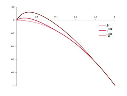
Figure 4: the second-best value function $v^{\text{$\rm SB$}}$, its barrier $F$ and the accident-free second-best value function $v^{\text{$\rm SB$}}_{0}$

Figure 4 illustrates the second-best value function $v^{\text{$\rm SB$}}$ and its barrier $F$, along with the second-best value function within the accident-free framework $v^{\text{$\rm SB$}}_{0}$. The latter obviously represents an upper bound for $v^{\text{$\rm SB$}}$ as the criterion of the principal is higher in the absence of accidents. While these two functions do not coincide over the entire half-line, it is evident that the features defining $v^{\text{$\rm SB$}}_{0}$ are transferred into the description of $v^{\text{$\rm SB$}}$. In other words, this parameter choice leads us to infer that the agent with a small reservation utility benefits from an informational rent because the principal optimally offers him a contract that gives utility strictly higher than his participation value. Furthermore, we can notice that the second-best value function $v^{\text{$\rm SB$}}$ does not coincide with its barrier ${F}$ in a neighbourhood of zero, but then becomes equal to it, indicating the existence of a golden parachute. This suggests that if the agent’s reservation utility is higher than the point where these functions intersect, the contract terminates immediately. In such a scenario, the agent exerts no effort but receives a positive lump-sum compensation since we are considering the case where both parties are equally impatient, resulting in $\bar{F}=F$.

To better understand how the second-best value function $v^{\text{$\rm SB$}}$ is affected by the accidents’ size, we compute this function for different values of $m$ while keeping the other parameters unchanged. Figure 5 clearly shows the convergence of $v^{\text{$\rm SB$}}$ to the second-best value function within the accident-free framework $v^{\text{$\rm SB$}}_{0}$ as $m$ decreases to 0. Furthermore, it is evident that as $m$ increases, the value function $v^{\text{$\rm SB$}}$ reaches the barrier $F$ sooner. This happens because, as $m$ becomes large, the size of potential accidents grows, leading the principal to decide earlier to terminate the contract due to her increased fear. Consequently, we can deduce that accidents significantly influence the second-best value function $v^{\text{$\rm SB$}}$ when the agent’s reservation utility is not too high. This occurs because in this case, the principal prefers to terminate the contract earlier than in the framework with fewer or no accidents. This preference arises from the increased cost associated with potential accidents, which exceeds the cost of offering the agent an immediate lump-sum compensation. This phenomenon is clearly visible in the zoomed-in box.

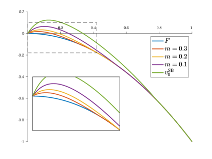
Figure 5: the second-best value function $v^{\text{$\rm SB$}}$ for different values of $m$

To conclude the analysis, we present in Table 1 the maximum values assumed by the functions $v^{\text{$\rm SB$}}_{0}$ and $v^{\text{$\rm SB$}}$ for different values of $m$. This helps us to better understand the loss in utility for the principal due to the presence of accidents. It is evident that as $m$ increases, the relative loss increases significantly. This phenomenon occurs because the larger the potential loss the principal could face, the more inclined she is to avoid risks and terminate the contract by compensating the agent with a lump-sum payment. It is worth noting that seemingly small values of $m$ can result in significant losses, approaching nearly 50%, as seen in the case of $m=0.1$.

	$v^{\text{$\rm SB$}}_{0}$	$m=0.1$	$m=0.2$	$m=0.3$
maximum value	0.1234	0.0648	0.0336	0.0176
relative loss	—	47.48%	72.75%	85.75%

Table 1: maximum value and relative loss for different values of $m$

To demonstrate that $m=0.1$ indeed represents a small value concerning potential accidents, we compare it against the average value assumed by the project’s value $X$ at the termination of the contract. Specifically, we simulate several paths of the project’s value $X$, whose dynamics under the optimal effort $\nu^{\star}=(\alpha^{\star},\beta^{\star})$ is given by

$$X_{t}=x_{0}+\int_{0}^{t}\alpha^{\star}_{s}\mathrm{d}s+\sigma W^{\nu^{\star}}_{t}-mN_{t},\;\text{\rm for}\;t\geq 0,$$

where the intensity of the Poisson process $N$ is $\int_{0}^{\cdot}(\beta^{\star}_{s}/m)\mathrm{d}s$. We consider $x_{0}=0$. Additionally, the optimal control $\nu^{\star}$ is associated with the continuation value of the agent $Y^{Y^{\text{$\rm A$}}_{\text{$0$}},\hat{Z}^{\text{$\rm A$}},\hat{U}^{\text{$\rm A$}},\hat{\pi}}$, whose dynamics is given in Equation 5.3. More precisely, $\hat{Z}^{{\rm A}}_{t}$ and $\hat{U}^{{\rm A}}_{t}$ are the maximisers of the operator $\mathcal{J}^{\text{$\rm SB$}}\big{(}Y^{{Y}^{\text{$\rm A$}}_{\text{$0$}},{\hat{Z}}^{\text{$\rm A$}},{\hat{U}}^{\text{$\rm A$}},{\hat{\pi}}}_{t},(v^{\text{$\rm SB$}})^{\prime}(Y^{{Y}^{\text{$\rm A$}}_{\text{$0$}},{\hat{Z}}^{\text{$\rm A$}},{\hat{U}}^{\text{$\rm A$}},{\hat{\pi}}}_{t}),(v^{\text{$\rm SB$}})^{\prime\prime}(Y^{{Y}^{\text{$\rm A$}}_{\text{$0$}},{\hat{Z}}^{\text{$\rm A$}},{\hat{U}}^{\text{$\rm A$}},{\hat{\pi}}}_{t}),v^{\text{$\rm SB$}}(\cdot))$, with associated optimal effort $\nu^{\star}_{t}=(\alpha^{\star}_{t},\beta^{\star}_{t})\in U^{\star}(Z^{{\rm A}}_{t},U^{{\rm A}}_{t})$, and $\hat{\pi}_{t}\coloneqq(F^{\star})^{\prime}((v^{\text{$\rm SB$}})^{\prime}(Y^{Y^{\text{$\rm A$}}_{\text{$0$}},\hat{Z}^{\text{$\rm A$}},\hat{U}^{\text{$\rm A$}},\hat{\pi}}_{t}))$. The termination of the contract then occurs at

$$\tau^{\star}\coloneqq\inf\big{\{}t\geq 0:\;v^{\text{$\rm SB$}}(Y^{Y^{\text{$\rm A$}}_{\text{$0$}},\hat{Z}^{\text{$\rm A$}},\hat{U}^{\text{$\rm A$}},\hat{\pi}}_{t})=F(Y^{Y^{\text{$\rm A$}}_{\text{$0$}},\hat{Z}^{\text{$\rm A$}},\hat{U}^{\text{$\rm A$}},\hat{\pi}}_{t})\big{\}}.$$

Since $Y^{\rm A}_{0}=V^{\rm A}$ (as explained in Remark 5.1.$(i)$), and Figure 5 indicates that the maximiser is $0.1011$ for $m=0.1$, we set $Y^{\rm A}_{0}=0.11$. Figure 6 illustrates several trajectories of the stopped project’s value $X^{\tau^{\text{$\star$}}}$ under the optimal effort $\nu^{\star}$ on the time horizon $[0,20]$, along with its average value. We select this time interval because less than 5% of the trajectories fail to reach the stopping region by that time, making the graph statistically significant. We can infer that the average value of $X$ at the time $\tau^{\star}$ is slightly below 4, indicating that $0.1$ is indeed small in comparison.

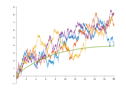
Figure 6: several trajectories depicting the project’s value $X$, under the optimal effort $\nu^{\star}$, and its average value

Appendix A Representation of the face-lifted utility

In this section, our objective is twofold: first, to deduce the form of the face-lifted utility $\bar{F}$ through an analysis of the Hamilton–Jacobi equation (3.1), and second, to establish that the conjectured function is indeed given by the mixed control–stopping problem. This is accomplished by means of a verification argument when the candidate solution exhibits sufficient regularity, or by invoking the dynamic programming principle in case where this regularity condition is not met.

A.1 An impatient agent and small average accident size

We assume that $\delta>1$ and $m\leq-F^{\star}(\delta F^{\prime}(0))$. The latter assumption implies that point $\bar{y}$ introduced in (3.4) is zero, and thus leads to the conclusion that the function $F$ cannot be a solution of the Hamilton–Jacobi equation (3.1). Hence, we focus our attention to the study of the following ODE:

$$F^{\star}\big{(}\delta w^{\prime}(y)\big{)}-\delta yw^{\prime}(y)+w(y)+m=0,\;y\in(0,\infty),\;w(0)=0.$$ (A.1)

In what follows, we adopt the same approach as in [44, Appendix A] to show that the utility $\bar{F}$ is a strictly concave solution to the previously introduced ODE, and it never touches the barrier $F$.

Lemma A.1.

If $w$ is a strictly concave continuously differentiable solution of Equation A.1, then $w^{\prime}(0)=f_{\delta m}$, where $f_{\delta m}\coloneqq(F^{\star})^{-1}(-m)/\delta$.

Proof.

If the right-derivative $w^{\prime}(0)$ is finite, the result follows by simply computing the limit for $y$ going to $0$ in (A.1). If we rather assume that $w^{\prime}(0)$ is not finite, specifically, $w^{\prime}(0)=\infty$ given the strict concavity of the function $w$, then there exists some $\varepsilon>0$ such that $w>0$ and $F^{\star}(\delta w^{\prime})=0$ on $(0,\varepsilon)$. Consequently, the following equation is satisfied:

$$-\delta yw^{\prime}(y)+w(y)+m=0,\;y\in(0,\varepsilon).$$

For any arbitrary $y_{0}\in(0,\varepsilon)$, the previous equation implies that

$$w(y)=\frac{w(y_{0})+m}{y_{0}^{\frac{1}{\delta}}}y^{\frac{1}{\delta}}-m\;\text{for any}\;y\in(y_{0},\varepsilon).$$

Given that $w(0)=0$, we deduce that $\lim_{y_{0}\rightarrow 0^{\text{$+$}}}(w(y_{0})+m)y_{0}^{-\frac{1}{\delta}}=\infty$. Then, $w=\infty$ on the interval $[0,\varepsilon)$, which contradicts the initial condition. ∎

Let us introduce the notation $w$ for a strictly concave and continuously differentiable solution to the ODE given in Equation A.1. Our goal is to derive the ODE that its concave conjugate $w^{\star}$ satisfies in order to deduce some properties that characterise $w^{\star}$, and consequently the function $w$ by standard convex duality. According to Alvarez, Lasry, and Lions [3, Proposition 5], the ODE that $w^{\star}$ satisfies is

$$F^{\star}(\delta p)+(1-\delta)p(w^{\star})^{\prime}(p)-w^{\star}(p)+m=0,\;p\in(-\infty,f_{\delta m}),\;w^{\star}(f_{\delta m})=0.$$ (A.2)

We can express the previous ODE in a linear form. As a result, based on, for instance, Ahmad and Ambrosetti [1, Corollary 2.2.11], we can uniquely determine the solution $w^{\star}$ by the following expression:

$$w^{\star}(p)=\frac{(-p)^{\frac{1}{1-\delta}}}{\delta-1}\int_{p}^{f_{\text{$\delta$}\text{$m$}}}\frac{F^{\star}(\delta x)}{(-x)^{1+\frac{1}{1-\delta}}}\mathrm{d}x+m\bigg{(}1-\bigg{(}\frac{p}{f_{\delta m}}\bigg{)}^{\frac{1}{1-\delta}}\bigg{)},\;\text{for}\;p\leq f_{\delta m}.$$ (A.3)

Proposition A.2.

It holds that $F^{\star}(p)\geq w^{\star}(p)$ for any $p\leq f_{\delta m}$. Moreover, $w^{\star}$ is strictly concave and increasing on $(-\infty,f_{\delta m})$.

Proof.

The condition imposed on the parameter $m$, specifically $m\leq-F^{\star}(\delta F^{\prime}(0))$, implies that $\bar{y}$, as introduced in (3.4), is equal to zero. Consequently,

$$-F^{\star}(p)+(1-\delta)p(F^{\star})^{\prime}(p)+F^{\star}(\delta p)+m\leq 0\;\text{for any}\;p\leq F^{\prime}(0)\leq f_{\delta m},$$

by standard convex duality (see [3, Proposition 5]). Additionally, if $F^{\prime}(0)<f_{\delta m}$, then $F^{\star}=0$ and $(F^{\star})^{\prime}=0$ on the interval $(F^{\prime}(0),f_{\delta m}]$. This observation, together with the fact that $f_{\delta m}=(F^{\star})^{-1}(-m)/\delta$, leads to the following inequality on the entire domain of definition of $w^{\star}$:

$$-F^{\star}(p)+(1-\delta)p(F^{\star})^{\prime}(p)+F^{\star}(\delta p)+m\leq 0,\;p\in(-\infty,f_{\delta m}].$$ (A.4)

By defining $\phi(p)\coloneqq(-p)^{-\frac{1}{1-\delta}}(F^{\star}(p)-w^{\star}(p))$, for $p\leq f_{\delta m}$, and using the fact that $w^{\star}$ satisfies (A.2), we derive that

$$\phi^{\prime}(p) =\frac{1}{1-\delta}(-p)^{-\frac{1}{1-\delta}-1}\big{(}F^{\star}(p)-w^{\star}(p)-p(1-\delta)((F^{\star})^{\prime}(p)-(w^{\star})^{\prime}(p)\big{)}$$

$$=\frac{1}{1-\delta}(-p)^{-\frac{1}{1-\delta}-1}\left(F^{\star}(p)-(1-\delta)p(F^{\star})^{\prime}(p)-F^{\star}(\delta p)-m\right).$$

It follows that the function $\phi$ is non-increasing because of (A.4). As a consequence, $F^{\star}$ is not below $w^{\star}$ on $(-\infty,f_{\delta m}]$ since

$$\phi(p)\geq\lim_{p\rightarrow f^{\text{$-$}}_{\text{$\delta$}\text{$m$}}}\phi(p)=(-f_{\delta m})^{-\frac{1}{1-\delta}}\big{(}F^{\star}(f_{\delta m})-w^{\star}(f_{\delta m})\big{)}=0\;\text{for any}\;p\leq f_{\delta m}.$$

We have showed that $F^{\star}(p)\geq w^{\star}(p)$ for any $p\leq f_{\delta m}$. However, it is still necessary to verify that the function $w^{\star}$ is strictly concave and to do this, we prove that its second derivative is negative by differentiating the ODE (A.2):

$$(1-\delta)^{2}p^{2}(w^{\star})^{\prime\prime}(p) =\delta\big{(}(1-\delta)p(w^{\star})^{\prime}(p)-(1-\delta)p(F^{\star})^{\prime}(\delta p)\big{)}$$

$$=\delta(w^{\star}(p)-F^{\star}(\delta p)-m-(1-\delta)p(F^{\star})^{\prime}(\delta p))\leq\delta(w^{\star}(p)-F^{\star}(p)-m)<0\;\text{for any}\;p<f_{\delta m}.$$

The fact that $w^{\star}$ is strictly concave on $(-\infty,f_{\delta m})$ implies that $w^{\star}$ is an increasing function since $w^{\star}(f_{\delta m})=0$, and it remains below $F^{\star}$, which is increasing on $(-\infty,F^{\prime}(0))$ and constant at $0$ on $[F^{\prime}(0),f_{\delta m}]$. ∎

Let us introduce the concave conjugate of $w^{\star}$, that is, $w^{\star\star}(y)\coloneqq\inf_{p\leq f_{\text{$\delta$}\text{$m$}}}\{yp-w^{\star}(p)\}$, for $y\geq 0$.

Proposition A.3.

Assuming that $\delta>1$ and $m\leq-F^{\star}(\delta F^{\prime}(0))$, and considering the unique solution $w^{\star}$ to Equation A.2, it holds that $w=w^{\star\star}$ is a solution to (3.1) and satisfies the growth condition $\bar{c}_{0}(-1-y^{\gamma})\leq w(y)\leq\bar{c}_{1}(1-y^{\gamma})$, $y\geq 0$, for some $(\bar{c}_{0},\bar{c}_{1})\in(0,\infty)^{2}$. Moreover, $w^{\prime}(0)=f_{\delta m}=(F^{\star})^{-1}(-m)/\delta$.

Proof.

The result Rockafellar [46, Theorem 12.2] shows that $w=w^{\star\star}$ due to the strict concavity of $w^{\star}$. This strict concavity property further implies the continuously differentiability of $w$, as demonstrated by [46, Theorem 26.6]. Finally, concave duality ensures the growth of $w$ from the growth condition of $w^{\star}$, and implies that $w$ is a solution of (A.1) but also of (3.1), given that $w\geq F^{\star\star}=F$ on the interval $[0,\infty)$. ∎

We can conclude this section by employing a standard verification argument to prove that the previously mentioned function $w$ indeed represents the face-lifted utility defined by the deterministic mixed control–stopping problem in (2.10).

Proof of Proposition 3.5.$(i)$.

We first show that $w$ is an upper bound for $\bar{F}$ on $[0,\infty)$. To this aim, we select a starting point $y_{0}\geq 0$, a control $p\in\mathcal{B}_{\mathbb{R}_{\text{$+$}}}$ and a stopping time $T\in[0,T^{y_{\text{$0$}},p}_{0}]$. Given that the function $w$ is not below $F$ on $[0,\infty)$, as proved in Proposition A.3, we have

$$w(y_{0}) =\mathrm{e}^{-\rho T}w(y^{y_{\text{$0$}},p}(T))\mathbf{1}_{\{T<\infty\}}+\int_{0}^{T}\rho\mathrm{e}^{-\rho t}\big{(}w(y^{y_{\text{$0$}},p}(t))-\delta w^{\prime}(y^{y_{\text{$0$}},p}(t))(y^{y_{0},p}(t)-p(t))\big{)}\mathrm{d}t$$

$$\geq\mathrm{e}^{-\rho T}F(y^{y_{\text{$0$}},p}(T))\mathbf{1}_{\{T<\infty\}}+\int_{0}^{T}\rho\mathrm{e}^{-\rho t}\big{(}F(p(t))-m\big{)}\mathrm{d}t,$$

due to the fact that $w$ solves Equation A.2. The arbitrariness of $p\in\mathcal{B}_{\mathbb{R}_{\text{$+$}}}$ and $T\in[0,T^{y_{\text{$0$}},p}_{0}]$ implies the desired inequality, that is, $w\geq F$ on the interval $[0,\infty)$.

To establish the converse inequality, let us fix some $y_{0}\geq 0$. We consider the maximiser in the definition of $F^{\star}(\delta w^{\prime}(y^{y_{\text{$0$}},p^{\star}}))$ as a feedback control, described by

$$\dot{y}^{y_{\text{$0$}},p^{\text{$\star$}}}(t)=r\big{(}y^{y_{\text{$0$}},p^{\text{$\star$}}}(t)-p^{\star}(t)\big{)},\;\text{where}\;p^{\star}(t)\coloneqq(F^{\star})^{\prime}\big{(}\delta w^{\prime}(y^{y_{\text{$0$}},p^{\text{$\star$}}}(t))\big{)},\;\text{for}\;t\geq 0.$$

It holds that

$$\dot{y}^{y_{\text{$0$}},p^{\text{$\star$}}}(t)=r\bigg{(}\frac{1-\delta}{\delta}\bigg{)}\frac{w^{\prime}(y^{y_{\text{$0$}},p^{\text{$\star$}}}(t))}{w^{\prime\prime}(y^{y_{\text{$0$}},p^{\text{$\star$}}}(t))}\;\text{for any}\;t>0.$$

Consequently, the trajectory $y^{y_{\text{$0$}},p^{\text{$\star$}}}$ is decreasing and thus remains well-defined until it reaches zero at its first hitting time $T^{\star}\coloneqq T^{y_{\text{$0$}},p^{\star}}_{0}<\infty$. The same calculations done in the first part of the proof lead to

$$w(y_{0})=\mathrm{e}^{-\rho T^{\star}}w\big{(}y^{y_{\text{$0$}},p^{\text{$\star$}}}(T^{\star})\big{)}+\int_{0}^{T^{\text{$\star$}}}\rho\mathrm{e}^{-\rho t}\big{(}F(p^{\star}(t))-m\big{)}\mathrm{d}t =\mathrm{e}^{-\rho T^{\text{$\star$}}}w(0)+\int_{0}^{T^{\text{$\star$}}}\rho\mathrm{e}^{-\rho t}\big{(}F(p^{\star}(t))-m\big{)}\mathrm{d}t$$

$$=\mathrm{e}^{-\rho T^{\text{$\star$}}}F(0)+\int_{0}^{T^{\text{$\star$}}}\rho\mathrm{e}^{-\rho t}\big{(}F(p^{\star}(t))-m\big{)}\mathrm{d}t$$

$$=\mathrm{e}^{-\rho T^{\text{$\star$}}}F(y^{y_{\text{$0$}},p^{\text{$\star$}}}(T^{\star}))+\int_{0}^{T^{\text{$\star$}}}\rho\mathrm{e}^{-\rho t}\big{(}F(p^{\star}(t))-m\big{)}\mathrm{d}t,$$

since $w(0)=0=F(0)$ by the boundary condition. We deduce that $(T^{\star},p^{\star})$ is an optimal control for the problem $\bar{F}$, thereby leading to the conclusion that the face-lifted utility $\bar{F}$ coincides with its upper bound $w$. ∎

A.2 When the agent is more impatient and the accidents’ size matters

Throughout this section, we investigate the mixed control–stopping problem (2.10) under the assumptions that $\delta>1$ and $m>-F^{\star}(\delta F^{\prime}(0))$. It is important to note that the latter assumption latter implies that $\bar{y}$ introduced in (3.4) is positive. In contrast to the previous section, it follows that $F$ can be a solution to the Hamilton–Jacobi equation (3.1) on a right-neighbourhood of zero. Indeed, this is precisely the case, as demonstrated by the following lemma for strictly concave solutions.

Lemma A.4.

For any strictly concave solution $w$ of Equation 3.1, there exists $\varepsilon>0$ such that $w$ coincides with $F$ on $[0,\varepsilon)$.

Proof.

Let us fix $\varepsilon>0$. We assume to the contrary that $w$ is a strictly concave solution of the Hamilton–Jacobi equation (3.1) such that it is above $F$ on $(0,\varepsilon)$. Consequently, it becomes a solution of Equation A.1 on the interval $(0,\varepsilon)$, leading to $w^{\prime}(0)=f_{\delta m}$, as inferred from Lemma A.1. The given hypothesis regarding the parameter $m$, that is, $F^{\star}(\delta F^{\prime}(0))>-m=F^{\star}(\delta f_{\delta m})$, implies that $w^{\prime}(0)<F^{\prime}(0)$. However, this contradicts the fact that $w>F$ on $(0,\varepsilon)$. ∎

Similar to the previous section, we now examine the equation solved by the concave conjugate $w^{\star}$ which is given by [3, Proposition 5] to be

$$-\min\Big{\{}(w^{\star})^{\prime}(p)p-w^{\star}(p)-F\big{(}(w^{\star})^{\prime}(p)\big{)},(1-\delta)p(w^{\star})^{\prime}(p)-w^{\star}(p)+F^{\star}(\delta p)+m\Big{\}}=0,\;p<F^{\prime}(0),\;w^{\star}(F^{\prime}(0))=0.$$ (A.5)

As we seek a strictly concave solution to the previous equation that coincides with $F^{\star}$ on the right-neighbourhood of $F^{\prime}(0)$ (as indicated by Lemma A.4), let us fix some $p_{\bar{y}}<F^{\prime}(0)$ and consider the function

$$w^{\star}(p)\coloneqq\begin{cases}w^{\star}_{\bar{y}}(p),\;p\in(-\infty,p_{\bar{y}})\\ F^{\star}(p),\;p\in[p_{\bar{y}},F^{\prime}(0)]\end{cases},$$ (A.6)

where $w^{\star}_{\bar{y}}$ is the unique solution of

$$-w^{\star}_{\bar{y}}(p)+(1-\delta)p(w^{\star}_{\bar{y}})^{\prime}(p)+F^{\star}(\delta p)+m=0,\;p\in(-\infty,p_{\bar{y}}),\;w^{\star}_{\bar{y}}(p_{\bar{y}})=F^{\star}(p_{\bar{y}}).$$ (A.7)

The solution to the equation above is explicitly given by

$$w^{\star}_{\bar{y}}(p)=\frac{(-p)^{\frac{1}{1-\delta}}}{\delta-1}\int_{p}^{p_{\text{$\bar{y}$}}}\frac{F^{\star}(\delta x)}{(-x)^{1+\frac{1}{1-\delta}}}\mathrm{d}x+\bigg{(}\frac{p}{p_{\bar{y}}}\bigg{)}^{\frac{1}{1-\delta}}(F^{\star}(p_{\bar{y}})-m)+m,\;\text{for}\;p\leq p_{\bar{y}}.$$ (A.8)

Lemma A.5.

The function described in (A.6) is continuously differentiable on $(-\infty,F^{\prime}(0))$ if and only if $p_{\bar{y}}=F^{\prime}(\bar{y})$.

Proof.

The function $w^{\star}$ is continuously differentiable if and only if

$$\frac{F^{\star}(\delta p_{\bar{y}})-F^{\star}(p_{\bar{y}})+m}{p_{\bar{y}}(\delta-1)}=(w^{\star}_{\bar{y}})^{\prime}(p_{\bar{y}})=(F^{\star})^{\prime}(p_{\bar{y}}).$$

The previous equality holds true if and only if

$$F^{\star}(p_{\bar{y}})-F^{\star}(\delta p_{\bar{y}})-m=w^{\star}_{\bar{y}}(p_{\bar{y}})-F^{\star}(\delta p_{\bar{y}})-m=(1-\delta)p_{\bar{y}}(w^{\star}_{\bar{y}})^{\prime}(p_{\bar{y}})=(1-\delta)p_{\bar{y}}(F^{\star})^{\prime}(p_{\bar{y}}).$$

By standard convex duality and in accordance with Assumption 3.2, there exists a unique $p_{\bar{y}}\leq F^{\prime}(0)$ for which the aforementioned equality is satisfied. Specifically, this is determined as $p_{\bar{y}}=F^{\prime}(\bar{y})$. ∎

Henceforth, we slightly abuse notations by setting $p_{\bar{y}}=F^{\prime}(\bar{y})$ in the definition of the function $w^{\star}$ as given in Equation A.6. Then, we proceed to outline several properties of this function $w^{\star}$ and prove this latter solves the conjugate obstacle problem. This, in turn, allows us to conclude that the concave conjugate of $w^{\star}$ coincides with the face-lifted function $\bar{F}$.

Remark A.6.

It holds that $w^{\star}\leq F^{\star}$ on $(-\infty,F^{\prime}(0)]$, and $w^{\star}$ is strictly concave and increasing on $(-\infty,F^{\prime}(0))$. These properties are evident on $[F^{\prime}(\bar{y}),F^{\prime}(0)]$ because $w^{\star}$ coincides with $F^{\star}$ on this interval, while can be proved with arguments similar to those presented in Proposition A.2 on $(-\infty,F^{\prime}(\bar{y}))$.

Proposition A.7.

The function $w^{\star}$ introduced in (A.6) satisfies Equation A.5.

Proof.

The function $w^{\star}$ is given by $F^{\star}$ on $[F^{\prime}(\bar{y}),F^{\prime}(0)]$. Within this interval, the following equations hold:

$$(F^{\star})^{\prime}(p)p-F^{\star}(p)-F((F^{\star})^{\prime}(p))=0,\;\text{and}\;-F^{\star}(p)+(1-\delta)p(F^{\star})^{\prime}(p)+F^{\star}(\delta p)+m\geq 0,$$

where the inequality is a consequence of the definition of $\bar{y}$ in (3.4). Then, we only need to show that the solution $w^{\star}_{\bar{y}}$ of the ODE (A.7) satisfies $(w^{\star}_{\bar{y}})^{\prime}(p)p-w^{\star}_{\bar{y}}(p)-F((w^{\star}_{\bar{y}})^{\prime}(p))\geq 0$ on $(-\infty,F^{\prime}(\bar{y}))$ in order to conclude the proof. However, this is verified because

$$(w^{\star}_{\bar{y}})^{\prime}(p)p-w^{\star}_{\bar{y}}(p)-F((w^{\star}_{\bar{y}})^{\prime}(p)) \geq(w^{\star}_{\bar{y}})^{\prime}(p)p-F^{\star}(p)-F((w^{\star}_{\bar{y}})^{\prime}(p))$$

$$\geq(w^{\star}_{\bar{y}})^{\prime}(p)p-F^{\star}(p)-\big{(}F((F^{\star})^{\prime}(p))+F^{\prime}((F^{\star})^{\prime}(p))((w^{\star}_{\bar{y}})^{\prime}(p)-(F^{\star})^{\prime}(p))\big{)}$$

$$=(w^{\star}_{\bar{y}})^{\prime}(p)(p-F^{\prime}((F^{\star})^{\prime}(p)))=0.$$

∎

Up to this point, we have investigated the properties of the function $w^{\star}$. Our current objective is to translate them into characteristics of its concave conjugate $w^{\star\star}$. By standard convex duality, the latter can be expressed as

$$w^{\star\star}(y)=\begin{cases}F(y),\;y\in[0,\bar{y}]\\ w_{\bar{y}}(y),\;y\in(\bar{y},\infty)\end{cases},$$ (A.9)

where $w_{\bar{y}}$ represents the concave conjugate of $w^{\star}_{\bar{y}}$ and thus satisfies

$$F^{\star}\big{(}\delta w^{\prime}_{\bar{y}}(y)\big{)}-\delta yw^{\prime}_{\bar{y}}(y)+w_{\bar{y}}(y)+m=0,\;y\in(\bar{y},\infty),\;w_{\bar{y}}(\bar{y})=F(\bar{y}),\;w^{\prime}_{\bar{y}}(\bar{y})=F^{\prime}(\bar{y}).$$ (A.10)

Proposition A.8.

Let $\delta>1$ and $m>-F^{\star}(\delta F^{\prime}(0))$. The function $w^{\star\star}$ introduced in (A.9) is a solution to the Hamilton–Jacobi equation (3.1) while satisfying the growth condition $\bar{c}_{0}(-1-y^{\gamma})\leq w^{\star\star}(y)\leq\bar{c}_{1}(1-y^{\gamma})$ for any $y\geq 0$, for some $(\bar{c}_{0},\bar{c}_{1})\in(0,\infty)^{2}$.

Proof.

As taking conjugates evidently reverses functional inequalities, it follows that $w^{\star\star}$ is always above $F$. This observation, together with the definition of $\bar{y}$, leads us to the conclusion that it is indeed a solution to Equation 3.1. Furthermore, concave duality ensures the growth of $w^{\star\star}$ in accordance with the growth condition established for $w^{\star}$. ∎

We can now present the main result of this section, which demonstrates that the aforementioned function $w^{\star\star}$ indeed represents the face-lifted utility $\bar{F}$.

Proof of Proposition 3.5.$(ii)$.

Similar to the proof of the statement in Proposition 3.5.$(i)$, we can show that $w^{\star\star}\geq\bar{F}$ on $[0,\infty)$. To prove the reverse inequality, we need to distinguish two distinct cases. Firstly, when $y_{0}\in[0,\bar{y}]$, the trivial control $(T^{\star},p^{\star}):=(0,0)$ is optimal as it attains the upper bound $w^{\star\star}(y_{0})$. This is straightforward to prove, as follows:

$$w^{\star\star}(y_{0})=\mathrm{e}^{-\rho T^{\star}}w^{\star\star}\big{(}y^{y_{\text{$0$}},p^{\star}}(T^{\star})\big{)}+\int_{0}^{T^{\text{$\star$}}}\rho\mathrm{e}^{-\rho t}\big{(}F(p^{\star}(t))-m\big{)}\mathrm{d}t=w^{\star\star}(y^{y_{\text{$0$}},p^{\text{$\star$}}}(0))=F\big{(}(y^{y_{\text{$0$}},p^{\text{$\star$}}}(0))\big{)}=F(y_{0}).$$

Next, we turn our attention to the case where $y_{0}>\bar{y}$. In this scenario, we define $p^{\star}(t)$ as the maximiser in the definition of $F^{\star}(\delta(\bar{F}^{\star\star})^{\prime}(y^{y_{\text{$0$}},p^{\text{$\star$}}}(t)))$, for $t\in[0,T^{\star}]$, where $T^{\star}\coloneqq\inf\{t\geq 0:y^{y_{\text{$0$}},p^{\text{$\star$}}}(t)\leq\bar{y}\}\in(0,T^{y_{\text{$0$}},p^{\text{$\star$}}}_{0})$. Consequently, the state dynamics is given by

$$\dot{y}^{y_{\text{$0$}},p^{\text{$\star$}}}(t)=r\bigg{(}\frac{1-\delta}{\delta}\bigg{)}\frac{(w^{\star\star})^{\prime}(y^{y_{\text{$0$}},p^{\text{$\star$}}}(t))}{(w^{\star\star})^{\prime\prime}(y^{y_{\text{$0$}},p^{\text{$\star$}}}(t))}\;\text{for any}\;t\in(0,T^{\star}).$$

It follows that $y^{y_{\text{$0$}},p^{\text{$\star$}}}$ is decreasing and, therefore, well-defined on $(0,T^{\star})$. Under the control $(T^{\star},p^{\star})$, it holds that

$$w^{\star\star}(y_{0})=\mathrm{e}^{-\rho T^{\text{$\star$}}}w^{\star\star}(y^{y_{\text{$0$}},p^{\text{$\star$}}}(T^{\star}))+\int_{0}^{T^{\text{$\star$}}}\rho\mathrm{e}^{-\rho t}\big{(}F(p^{\star}(t))-m\big{)}\mathrm{d}t =\mathrm{e}^{-\rho T^{\text{$\star$}}}F(\bar{y})+\int_{0}^{T^{\text{$\star$}}}\rho\mathrm{e}^{-\rho t}\big{(}F(p^{\star}(t))-m\big{)}\mathrm{d}t$$

$$=\mathrm{e}^{-\rho T^{\text{$\star$}}}F(y^{y_{0},p^{\star}}(T^{\star}))+\int_{0}^{T^{\text{$\star$}}}\rho\mathrm{e}^{-\rho t}\big{(}F(p^{\star}(t))-m\big{)}\mathrm{d}t.$$

Here, we have used the fact that $y^{y_{\text{$0$}},p^{\text{$\star$}}}(T^{\star})=\bar{y}$ and that $v_{\bar{y}}(\bar{y})=F(\bar{y})$. We deduce that $(T^{\star},p^{\star})$ is an optimal control for the problem $\bar{F}$ when $y_{0}>\bar{y}$. This concludes the proof. ∎

A.3 When the principal becomes impatient, but not too much

We assume that $\delta<1$ and $\gamma\delta>1$. Reasoning analogous to that developed in Lemma A.4 suggests that any solution $w$ to the Hamilton-Jacobi equation (3.1) coincides with the function $F$ on $[0,\varepsilon)$ for some $\varepsilon>0$. Furthermore, $w$ is continuously differentiable only when it equals $F$ on the non-degenerate interval $[0,\bar{y}]$ (it is important to highlight that $\bar{y}$ is positive under the assumptions of this section). However, this choice is inadmissible since it leads to a solution $w$ that falls below the barrier $F$ on a right-neighbourhood of $\bar{y}$. Therefore, we propose the ansatz that $w$ takes the form outlined in Proposition 3.10. Given that the suggested function $w$ fails to be differentiable everywhere, our next results necessitate the use of the theory of viscosity solutions. For a more comprehensive treatment in the case of Hamilton–Jacobi equations, we refer the reader to Lions [34].

Proposition A.9.

Assuming $\delta<1$ and $\gamma\delta>1$, the function

$$v_{\tilde{y}}(y)\coloneqq\begin{cases}F(y),\;y\in[0,\tilde{y}]\\ w_{0}(y)-m,\;y\in(\tilde{y},\infty)\end{cases},$$

becomes a viscosity solution to the Hamilton–Jacobi equation (3.1). Here, $w_{0}$ denotes the face-lifted utility that is introduced in [44, Proposition 2.1] and readdressed in Equation 3.6, while $\tilde{y}$ is defined in Lemma 3.9. Additionally, we have that $\bar{c}_{0}(-1-y^{\gamma})\leq v_{\tilde{y}}(y)\leq\bar{c}_{1}(1-y^{\gamma})$, for $y\geq 0$, for some $(\bar{c}_{0},\bar{c}_{1})\in(0,\infty)^{2}$.

Proof.

Firstly, it is important to note that the growth condition directly follows from [44, Proposition 2.1]. Subsequently, as highlighted in Lemma 3.9, the function $v_{\tilde{y}}$ is continuous on $(0,\infty)$ and continuously differentiable on the same interval, except at the point $\tilde{y}>0$, by definition. We can then prove that $v_{\tilde{y}}$ satisfies the Hamilton–Jacobi equation (3.1) in three distinct steps based on the interval of the non-negative half-line under consideration. Initially, it is trivial that $v_{\tilde{y}}$ solves Equation 3.1 on $(0,\tilde{y})$ since $\tilde{y}<\bar{y}$. The proof is also straightforward on $(\tilde{y},\infty)$, given that $w_{\tilde{y}}$ is a solution to the ODE (3.7). It is only sufficient to check whether $v_{\tilde{y}}$ is above $F$ on that interval but this is simply verified. In fact, the proof of Lemma 3.9 implies that the function $v_{\tilde{y}}-F=w_{0}-m-F$ is increasing on $(\tilde{y},\infty)$ and $(v_{\tilde{y}}-F)(\tilde{y})=0$.

Lastly, the proof of the viscosity solution property of $v_{\tilde{y}}$ at $\tilde{y}$ requires our focus on examining the super-differential $D^{+}v_{\tilde{y}}(\tilde{y})$ and the sub-differential $D^{-}v_{\tilde{y}}(\tilde{y})$ of the function at that particular point, see for instance Bardi and Capuzzo-Dolcetta [6, Lemma I.1.7]. As a direct consequence of this result, the viscosity super-solution property of $v_{\tilde{y}}$ at $\tilde{y}$ turns out to be equivalent to the following condition:

$$\min\left\{v_{\tilde{y}}(\tilde{y})-F(\tilde{y}),F^{\star}(\delta p)-\delta\tilde{y}p+v_{\tilde{y}}(\tilde{y})+m\right\}=\min\left\{0,F^{\star}(\delta p)-\delta\tilde{y}p+w_{0}(\tilde{y})\right\}\geq 0\;\text{for any}\;p\in D^{-}v_{\tilde{y}}(\tilde{y}).$$ (A.11)

Therefore, Equation A.11 is verified if and only if $F^{\star}(\delta p)-\delta\tilde{y}p+w_{0}(\tilde{y})\geq 0$ for any $p\in D^{-}v_{\tilde{y}}(\tilde{y})$. This condition is derived straightforwardly from the fact that the function $[F^{\prime}(\tilde{y}),w_{0}^{\prime}(\tilde{y})]\ni p\longmapsto F^{\star}(\delta p)-\delta\hat{y}p+w_{0}(\tilde{y})$ is decreasing and is null at $w_{0}^{\prime}(\tilde{y})$ due to the ODE satisfied by $w_{0}$, while $D^{-}v_{\tilde{y}}(\tilde{y})=\{p\in\mathbb{R}:F^{\prime}(\tilde{y})\leq p\leq w^{\prime}_{0}(\tilde{y})\}$. However, the proof of this last assertion is deferred to the end for the sake of clarity. Consequently, we can conclude that $v_{\tilde{y}}$ constitutes a viscosity solution of the Hamilton–Jacobi equation (3.1) at $\tilde{y}$ because [6, Lemma II.1.8] implies that the super-differential $D^{+}v_{\tilde{y}}(\tilde{y})$ is empty due to the function not being continuously differentiable at that specific point.

To complete the proof, it remains to prove the claim $D^{-}v_{\tilde{y}}(\tilde{y})=\{p\in\mathbb{R}:F^{\prime}(\tilde{y})\leq p\leq w^{\prime}_{0}(\tilde{y})\}$. For any $p>w^{\prime}_{0}(\tilde{y})$, it is evident that

$$\liminf_{y\rightarrow\tilde{y}}\bigg{\{}\frac{v_{\tilde{y}}(y)-v_{\tilde{y}}(\tilde{y})-p(y-\tilde{y})}{|\tilde{y}-y|}\bigg{\}}\leq\liminf_{y\rightarrow\tilde{y}^{\text{$+$}}}\bigg{\{}\frac{w_{0}(y)-w_{0}(\tilde{y})-p(y-\tilde{y})}{|\tilde{y}-y|}\bigg{\}}\leq w^{\prime}_{0}(\tilde{y})-p<0.$$

Here, we have used the fact that the function $w_{0}$ is strictly concave on its domain of definition. Therefore, it follows that $p\notin D^{-}v_{\tilde{y}}(\tilde{y})$, and the same conclusion holds for any $p<F^{\prime}(\tilde{y})$:

$$\liminf_{y\rightarrow\tilde{y}}\bigg{\{}\frac{v_{\tilde{y}}(y)-v_{\tilde{y}}(\tilde{y})-p(y-\tilde{y})}{|\tilde{y}-y|}\bigg{\}}\leq\liminf_{y\rightarrow\tilde{y}^{\text{$-$}}}\bigg{\{}\frac{F(y)-F(\tilde{y})-p(y-\tilde{y})}{|\tilde{y}-y|}\bigg{\}}\leq p-F^{\prime}(\tilde{y})<0,$$

taking into account the concavity of $F$. For any $p\in[F^{\prime}(\tilde{y}),w^{\prime}(\tilde{y})]$, let us define the continuously differentiable function

$$\phi_{p}(y)\coloneqq F(\tilde{y})+p(y-\tilde{y})-(y-\tilde{y})^{\frac{1}{\gamma}},\;\text{for}\;y\geq 0.$$

We can justify that $\tilde{y}$ is a local minimum of the difference $v_{\tilde{y}}-\phi_{p}$ because $p$ falls within the interval $[(v_{\tilde{y}})_{-}^{\prime}(\tilde{y}),(v_{\tilde{y}})_{+}^{\prime}(\tilde{y})]=[F^{\prime}(\tilde{y}),0]$. According to [6, Lemma II.1.7], it follows that $p\in D^{-}v_{\tilde{y}}(\tilde{y})$. ∎

We have just proved that $v_{\tilde{y}}$ is a viscosity solution of the Hamilton–Jacobi equation (3.1). Next, we proceed to show that the function $\bar{F}$, defined as the solution to the mixed control-stopping problem in (2.10), also satisfies the same equation in the viscosity sense. Subsequently, by invoking a comparison theorem, we can effectively characterise $\bar{F}$ as the unique viscosity solution, with appropriate growth at infinity. This guarantees the equivalence of the two aforementioned functions. To this aim, we introduce the following result, which is fundamental for characterising $\bar{F}$ as a viscosity solution of Equation 2.10, as proven in Proposition A.11 below.

Lemma A.10.

Let us fix some $y_{0}\geq 0$. For any time $\theta\geq 0$, it holds that

$$\bar{F}(y_{0}) \leq\sup_{p\in\mathcal{B}_{\text{$\mathbb{R}$}_{\text{$+$}}}}\sup_{T\in[0,T^{\text{$y$}_{\text{$0$}}\text{$,$}\text{$p$}}_{\text{$0$}}]}\bigg{\{}\int_{0}^{T\wedge\theta}\rho\mathrm{e}^{-\rho t}(-m+F(p(t)))\mathrm{d}t+\mathrm{e}^{-\rho T}F(y^{y_{\text{$0$}},p}(T))\mathbf{1}_{\{T<\theta\}}+\mathrm{e}^{-\rho\theta}\bar{F}^{s}(y^{y_{\text{$0$}},p}(\theta))\mathbf{1}_{\{T\geq\theta\}}\bigg{\}}$$

$$\bar{F}(y_{0}) \geq\sup_{p\in\mathcal{B}_{\text{$\mathbb{R}$}_{\text{$+$}}}}\sup_{T\in[0,T^{\text{$y$}_{\text{$0$}}\text{$,$}\text{$p$}}_{\text{$0$}}]}\bigg{\{}\int_{0}^{T\wedge\theta}\rho\mathrm{e}^{-\rho t}\big{(}-m+F(p(t))\big{)}\mathrm{d}t+\mathrm{e}^{-\rho T}F(y^{y_{\text{$0$}},p}(T))\;\mathbf{1}_{\{T<\theta\}}+\mathrm{e}^{-\rho\theta}\bar{F}_{i}(y^{y_{\text{$0$}},p}(\theta))\;\mathbf{1}_{\{T\geq\theta\}}\bigg{\}}.$$

Here, the functions $\bar{F}^{s}$ and $\bar{F}_{i}$ denote the upper–semi-continuous and the lower–semi-continuous envelope of $\bar{F}$, respectively.

Proof.

Let us consider some $p\in\mathcal{B}_{\mathbb{R}_{+}}$ and $T\in[0,T^{y_{\text{$0$}},p}_{0}]$, and denote

$$f^{y_{\text{$0$}}}(p,T)\coloneqq \int_{0}^{T}\rho\mathrm{e}^{-\rho t}\big{(}-m+F(p(t))\big{)}\mathrm{d}t+\mathrm{e}^{-\rho T}F\big{(}y^{y_{\text{$0$}},p}(T)\big{)}\mathbf{1}_{\{T<\infty\}}.$$

It follows that

$$f^{y_{\text{$0$}}}(p,T) =f^{y_{\text{$0$}}}(p,T)\mathbf{1}_{\{T<\theta\}}$$

$$\quad+\bigg{(}\int_{0}^{\theta}\rho\mathrm{e}^{-\rho t}\big{(}-m+F(p(t))\big{)}\mathrm{d}t+\int_{\theta}^{T}\rho\mathrm{e}^{-\rho t}\big{(}-m+F(p(t))\big{)}\mathrm{d}t+\mathrm{e}^{-\rho T}F\big{(}y^{y_{\text{$0$}},p}(T)\big{)}\mathbf{1}_{\{T<\infty\}}\bigg{)}\mathbf{1}_{\{T\geq\theta\}}$$

$$=f^{y_{\text{$0$}}}(p,T)\mathbf{1}_{\{T<\theta\}}+\bigg{(}\int_{0}^{\theta}\rho\mathrm{e}^{-\rho t}\big{(}-m+F(p(t))\big{)}\mathrm{d}t\bigg{)}\mathbf{1}_{\{T\geq\theta\}}$$

$$\quad+\mathrm{e}^{-\rho\theta}\bigg{(}\int_{0}^{T-\theta}\rho\mathrm{e}^{-\rho t}\big{(}-m+F(\tilde{p}(t))\big{)}\mathrm{d}t+\mathrm{e}^{-\rho(T-\theta)}F\big{(}y^{{y^{\text{$y$}_{\text{$0$}}\text{$,$}\text{$p$}}(\theta)},\tilde{p}}(T-\theta)\big{)}\mathbf{1}_{\{T<\infty\}}\bigg{)}\mathbf{1}_{\{T\geq\theta\}},$$

where $\tilde{p}(t)\coloneqq p(t-\theta)$, for $t\geq 0$. Since $\tilde{p}\in\mathcal{B}_{\mathbb{R}_{\text{$+$}}}$, we have

$$f^{y_{\text{$0$}}}(p,T) \leq f^{y_{\text{$0$}}}(p,T)\mathbf{1}_{\{T<\theta\}}+\bigg{(}\int_{0}^{\theta}\rho\mathrm{e}^{-\rho t}\big{(}-m+F(p(t))\big{)}\mathrm{d}t+\mathrm{e}^{-\rho\theta}\bar{F}^{s}(y^{y_{\text{$0$}},p}(\theta))\bigg{)}\mathbf{1}_{\{T\geq\theta\}}.$$

We deduce that the first inequality simply follows by taking the supremum over $p\in\mathcal{B}_{\mathbb{R}_{\text{$+$}}}$ and $T\in\left[0,T^{y_{\text{$0$}},p}_{0}\right]$. In order to prove the second inequality, let us fix $\varepsilon>0$. For any $y\geq 0$, there exist some $p^{\varepsilon,y}\in\mathcal{B}_{\mathbb{R}_{\text{$+$}}}$ and $T^{\varepsilon,y}\in[0,T^{y,p^{\text{$\varepsilon$}\text{$,$}\text{$y$}}}_{0}]$ such that

$$\int_{0}^{T^{\text{$\varepsilon$}\text{$,$}\text{$y$}}}\rho\mathrm{e}^{-\rho t}\big{(}-m+F(p^{\varepsilon,y}(t))\big{)}\mathrm{d}t+\mathrm{e}^{-\rho T^{\text{$\varepsilon$}\text{$,$}\text{$y$}}}F\big{(}y^{y,p^{\text{$\varepsilon$}\text{$,$}\text{$y$}}}(T^{\varepsilon,y})\big{)}\mathbf{1}_{\{T^{\text{$\varepsilon$}\text{$,$}\text{$y$}}<\infty\}}\geq\bar{F}_{i}(y)-\varepsilon.$$ (A.12)

Let us fix $p\in\mathcal{B}_{\mathbb{R}_{\text{$+$}}}$ and $T\in[0,T^{y_{\text{$0$}},p}_{0}]$. It holds that

$$\bar{F}(y_{0}) \geq f^{y_{\text{$0$}}}(p,T)\mathbf{1}_{\{T<\theta\}}+\bigg{(}\int_{0}^{\theta+T^{\text{$\varepsilon$}\text{$,$}\text{$y$}^{\text{$y$}_{\text{$0$}}\text{$,$}\text{$p$}}(\theta)}}\rho\mathrm{e}^{-\rho t}\big{(}-m+F(\tilde{p}^{\varepsilon,y^{y_{\text{$0$}},p}(\theta)}(t))\big{)}\mathrm{d}t\bigg{)}\mathbf{1}_{\{T\geq\theta\}}$$

$$\quad+\mathrm{e}^{-\rho(\theta+T^{\text{$\varepsilon$}\text{$,$}\text{$y$}^{\text{$y$}_{\text{$0$}}\text{$,$}\text{$p$}}(\theta)})}F\Big{(}y^{y_{\text{$0$}},\tilde{p}^{\text{$\varepsilon$}\text{$,$}\text{$y$}^{\text{$y$}_{\text{$0$}}\text{$,$}\text{$p$}}(\theta)}}\big{(}\theta+T^{\text{$\varepsilon$}\text{$,$}\text{$y$}^{\text{$y$}_{\text{$0$}}\text{$,$}\text{$p$}}(\theta)}\big{)}\Big{)}\mathbf{1}_{\{T^{\text{$\varepsilon$}\text{$,$}\text{$y$}^{\text{$y$}_{\text{$0$}}\text{$,$}\text{$p$}}(\theta)}<\infty\}}\mathbf{1}_{\{T\geq\theta\}},$$

where

$$\tilde{p}^{\varepsilon,y^{\text{$y$}_{\text{$0$}}\text{$,$}\text{$p$}}(\theta)}(t)\coloneqq\begin{cases}p(t),\;t\in[0,\theta)\\ p^{\varepsilon,y^{\text{$y$}_{\text{$0$}}\text{$,$}\text{$p$}}(\theta)}(t-\theta),\;t\in[\theta,\infty)\end{cases}.$$

As $\tilde{p}^{\varepsilon}\in\mathcal{B}_{\mathbb{R}_{\text{$+$}}}$ and $\theta+T^{\varepsilon,y^{\text{$y$}_{\text{$0$}}\text{$,$}\text{$p$}}_{\theta}}\in[0,T^{y_{\text{$0$}},\tilde{p}^{\varepsilon}}_{0}]$, we can apply the previous inequality (A.12) to get

$$\bar{F}(y_{0}) \geq\int_{0}^{T\wedge\theta}\rho\mathrm{e}^{-\rho t}\big{(}-m+F(p(t))\big{)}\mathrm{d}t+\mathrm{e}^{-\rho T}F(y^{y_{\text{$0$}},p}(T))\mathbf{1}_{\{T<\theta\}}$$

$$\quad+\bigg{(}\mathrm{e}^{-\rho\theta}\int_{\theta}^{\theta+T^{\text{$\varepsilon$}\text{$,$}\text{$y$}^{\text{$y$}_{\text{$0$}}\text{$,$}\text{$p$}}(\theta)}}\rho\mathrm{e}^{-\rho(t-\theta)}\big{(}-m+F(p^{\varepsilon,y^{y_{\text{$0$}},p}(\theta)}(t-\theta))\big{)}\mathrm{d}t\bigg{)}\mathbf{1}_{\{T\geq\theta\}}$$

$$\quad+\mathrm{e}^{-\rho\theta}\mathrm{e}^{-\rho T^{\text{$\varepsilon$}\text{$,$}\text{$y$}^{\text{$y$}_{\text{$0$}}\text{$,$}\text{$p$}}(\theta)}}F\Big{(}y^{y^{\text{$y$}_{\text{$0$}}\text{$,$}\text{$p$}}(\theta),p^{\text{$\varepsilon$}\text{$,$}\text{$y$}^{\text{$y$}_{\text{$0$}}\text{$,$}\text{$p$}}(\theta)}}\big{(}T^{\varepsilon,y^{\text{$y$}_{\text{$0$}}\text{$,$}\text{$p$}}(\theta)}\big{)}\Big{)}\mathbf{1}_{\{T^{\text{$\varepsilon$}\text{$,$}\text{$y$}^{\text{$y$}_{\text{$0$}}\text{$,$}\text{$p$}}(\theta)}<\infty\}}\mathbf{1}_{\{T\geq\theta\}}$$

$$\geq\int_{0}^{T\wedge\theta}\rho\mathrm{e}^{-\rho t}\big{(}-m+F(p(t))\big{)}\mathrm{d}t+\mathrm{e}^{-\rho T}F\big{(}y^{y_{\text{$0$}},p}(T)\big{)}\;\mathbf{1}_{\{T<\theta\}}+\big{(}\bar{F}_{i}(y^{y_{\text{$0$}},p}(\theta))-\varepsilon\big{)}\mathbf{1}_{\{T\geq\theta\}}.$$

The conclusion follows by taking the supremum over $p\in\mathcal{B}_{\mathbb{R}_{\text{$+$}}}$ and $T\in[0,T^{y_{\text{$0$}},p}_{0}]$, and then by sending $\varepsilon$ to zero. ∎

Proposition A.11.

The function $\bar{F}$ is a viscosity solution of the Hamilton–Jacobi equation (3.1).

Proof.

Starting from the evident inequality $\bar{F}-F\geq 0$ on $[0,\infty)$, it follows immediately that $\bar{F}_{i}-F\geq 0$ on the same interval. Thus, it suffices to prove that $\bar{F}$ is a viscosity super-solution of the ODE presented in (3.1) to show the super-solution property. Let us fix a smooth test function $\phi$ and $y^{0}\geq 0$ such that $y^{0}$ is a local minimum point for the difference $\bar{F}_{i}-\phi$ on $[0,\infty)$, with $(\bar{F}_{i}-\phi)(y^{0})=0$. Then, by definition of $\bar{F}_{i}$, there exists a non-negative sequence $(y_{n})_{n\in\mathbb{N}}$ such that

$$y_{n}\underset{n\to\infty}{\longrightarrow}y^{0},\;\bar{F}(y_{n})\underset{n\to\infty}{\longrightarrow}\bar{F}_{i}(y^{0}),\;\bar{F}(y_{n})-\phi(y_{n})\underset{n\to\infty}{\longrightarrow}0.$$

Consequently, we can define a positive sequence $(h_{n})_{n\in\mathbb{N}}$ by

$$h_{n}\coloneqq|\bar{F}(y_{n})-\phi(y_{n})|^{\frac{1}{2}}\;\mathbf{1}_{\{|\bar{F}(y_{\text{$n$}})-\phi(y_{\text{$n$}})|>0\}}+\frac{1}{n}\;\mathbf{1}_{\{|\bar{F}(y_{\text{$n$}})-\phi(y_{\text{$n$}})|=0\}},\;\text{for}\;n\in\mathbb{N}.$$ (A.13)

It is true that

$$h_{n}\underset{n\to\infty}{\longrightarrow}0,\;\frac{\bar{F}(y_{n})-\phi(y_{n})}{h_{n}}\underset{n\to\infty}{\longrightarrow}0.$$

The second inequality of Lemma A.10 implies that, for any $p\in\mathcal{B}_{\mathbb{R}_{\text{$+$}}}$ and sufficiently small values of $h_{n}$,

$$\bar{F}(y_{n}) \geq\int_{0}^{h_{n}}\rho\mathrm{e}^{-\rho t}\big{(}-m+F(p(t))\big{)}\mathrm{d}t+\mathrm{e}^{-\rho h_{\text{$n$}}}\bar{F}_{i}(y^{y_{\text{$n$}},p}(h_{n}))$$

$$\geq\int_{0}^{h_{n}}\rho\mathrm{e}^{-\rho t}\big{(}-m+F(p(t))\big{)}\mathrm{d}t+\mathrm{e}^{-\rho h_{\text{$n$}}}\phi(y^{y_{\text{$n$}},p}(h_{n}))$$

$$=\int_{0}^{h_{n}}\rho\mathrm{e}^{-\rho t}\big{(}-m+F(p(t))\big{)}\mathrm{d}t+\bigg{(}\phi(y_{n})+\int_{0}^{h_{n}}\rho\mathrm{e}^{-\rho t}\big{(}-\phi(y^{y_{\text{$n$}},p}(t))+\delta\phi^{\prime}(y^{y_{\text{$n$}},p}(t))(y^{y_{\text{$n$}},p}(t)-p(t))\big{)}\mathrm{d}t\bigg{)}.$$

Here, the second inequality follows directly from the local minimiser property of $\tilde{y}$, while the last equality is a consequence of the fundamental theorem of calculus. It follows that

$$\frac{\bar{F}(y_{n})-\phi(y_{n})}{h_{n}}+\frac{1}{h_{n}}\int_{0}^{h_{n}}\rho\mathrm{e}^{-\rho t}\big{(}m-F(p(t))+\phi(y^{y_{\text{$n$}},p}(t))-\delta\phi^{\prime}(y^{y_{\text{$n$}},p}(t))(y^{y_{\text{$n$}},p}(t)-p(t))\big{)}\mathrm{d}t\geq 0$$

and, by taking the limit for $n$ going to $\infty$, we get that

$$m-F(p(0))+\phi(y^{0})-\delta\phi^{\prime}(y^{0})(y^{0}-p(0))\geq 0\;\text{for any}\;p\in\mathcal{B}_{\mathbb{R}_{\text{$+$}}}.$$

The super-solution property is therefore proved due to the arbitrariness of $p\in\mathcal{B}_{\mathbb{R}_{\text{$+$}}}$. Subsequently, we show that $\bar{F}$ is a sub-solution by contradiction. As before, we select a smooth test function $\phi$ and $y^{0}\geq 0$ such that $y^{0}$ is a point of local maximum for $\bar{F}^{s}-\phi$, with $(\bar{F}^{s}-\phi)(y^{0})=0$. By contradiction, we assume that

$$\phi(y^{0})-F(y^{0})>0,\;\text{and}\;F^{\star}(\delta\phi^{\prime}(y^{0}))-\delta\phi^{\prime}(y^{0})y^{0}+\phi(y^{0})+m>0.$$

Let us fix $\varepsilon>0$. The definition of $\bar{F}^{s}$ implies the existence of a sequence $(y_{n})_{n\in\mathbb{N}}$ taking values in $(\tilde{y}-\varepsilon,\tilde{y}+\varepsilon)\cap[0,\infty)$ such that

$$y_{n}\underset{n\to\infty}{\longrightarrow}y^{0},\;\bar{F}(y_{n})\underset{n\to\infty}{\longrightarrow}\bar{F}^{s}(y^{0}),\;\bar{F}(y_{n})-\phi(y_{n})\underset{n\to\infty}{\longrightarrow}0.$$

As in (A.13), we can construct a positive sequence $(h_{n})_{n\in\mathbb{N}}$ satisfying

$$h_{n}\underset{n\to\infty}{\longrightarrow}0,\;\frac{\bar{F}(y_{n})-\phi(y_{n})}{h_{n}}\underset{n\to\infty}{\longrightarrow}0.$$

Then, the first inequality in Lemma A.10 implies that, for sufficiently small values of $h_{n}$, there exists $p^{\varepsilon}\in\mathcal{B}_{\mathbb{R}_{+}}$ such that

$$\bar{F}(y_{n})-\varepsilon h_{n} \leq\int_{0}^{h_{n}}\rho\mathrm{e}^{-\rho t}\big{(}-m+F(p^{\varepsilon}(t))\big{)}\mathrm{d}t+\mathrm{e}^{-\rho h_{n}}\bar{F}^{s}\big{(}y^{y_{\text{$n$}},p^{\text{$\varepsilon$}}}(h_{n})\big{)}$$

$$\leq\int_{0}^{h_{n}}\rho\mathrm{e}^{-\rho t}\big{(}-m+F(p^{\varepsilon}(t))\big{)}\mathrm{d}t+\mathrm{e}^{-\rho h_{n}}\phi\big{(}y^{y_{\text{$n$}},p^{\text{$\varepsilon$}}}(h_{n}))$$

$$=\int_{0}^{h_{n}}\rho\mathrm{e}^{-\rho t}\big{(}-m+F(p^{\varepsilon}(t))\big{)}\mathrm{d}t+\phi(y_{n})+\int_{0}^{h_{n}}\rho\mathrm{e}^{-\rho t}\big{(}-\phi(y^{y_{\text{$n$}},p^{\text{$\varepsilon$}}}(t))+\delta\phi^{\prime}(y^{y_{\text{$n$}},p^{\text{$\varepsilon$}}}(t))(y^{y_{\text{$n$}},p^{\text{$\varepsilon$}}}(t)-p^{\varepsilon}(t))\big{)}\mathrm{d}t.$$

It follows that

$$\frac{\bar{F}(y_{n})-\phi(y_{n})}{h_{n}}-\varepsilon+\frac{1}{h_{n}}\int_{0}^{h_{n}}\rho\mathrm{e}^{-\rho t}\big{(}m-F(p^{\varepsilon}(t))+\phi(y^{y_{\text{$n$}},p^{\text{$\varepsilon$}}}(t))-\delta\phi^{\prime}(y^{y_{\text{$n$}},p^{\text{$\varepsilon$}}}(t))(y^{y_{\text{$n$}},p^{\text{$\varepsilon$}}}(t)-p^{\varepsilon}(t))\big{)}\mathrm{d}t\leq 0.$$

Additionally, the mean-value theorem implies that

$$-\varepsilon+\rho\big{(}m-F(p^{\varepsilon}(0))+\phi(y^{0})-\delta\phi^{\prime}(y^{0})(y^{0}-p^{\varepsilon}(0))\big{)}\leq 0.$$

We get the desired contradiction by taking the limit for $\varepsilon$ going to zero. ∎

After showing that $\bar{F}$ is a viscosity solution of the Hamilton–Jacobi equation (3.1), we can infer its equivalence with $v_{\tilde{y}}$ as defined in Proposition A.9. This conclusion is attained through the following result that relies on the application of the comparison theorem for the aforementioned equation in Proposition A.12.

Proof of Proposition 3.10.$(i)$.

Proposition A.11 proves that $\bar{F}^{s}$ is an upper–semi-continuous viscosity sub-solution of (3.1), whereas $\bar{F}_{i}$ is a lower–semi-continuous viscosity super-solution. The comparison result stated in Proposition A.12 further indicates that $\bar{F}^{s}\leq\bar{F}_{i}$, leading to the conclusion that the function $\bar{F}$ is continuous on its domain of definition. It follows that $\bar{F}$ is the unique viscosity solution of the equation (3.1) within an appropriate class of functions with a given growth condition. Moreover, Proposition A.9 implies that $\bar{F}=v_{\tilde{y}}$ on $[0,\infty)$. ∎

Proposition A.12.

Let $u$ be an upper–semi-continuous viscosity sub-solution and $v$ be a lower–semi-continuous viscosity super-solution to Equation 3.1 so that there exists $(\bar{c}_{0},\bar{c}_{1})\in(0,\infty)^{2}$ satisfying

$$-\bar{c}_{0}(1+y^{\gamma})\leq\phi(y)\leq\bar{c}_{1}(1-y^{\gamma}),\;y\geq 0,\;\text{for}\;\phi\in\{u,v\}.$$

If $u(0)=0=v(0)$, then $u\leq v$ on $[0,\infty)$.

Proof.

By contradiction, we assume that there exists some $y^{\text{$\Delta$}}\in(0,\infty)$ such that $(u-v)(y^{\text{$\Delta$}})>0$. Let us fix $\varepsilon>0$. We introduce a positive and non-decreasing sequence $(\alpha_{n})_{n\in\mathbb{N}}$ such that $\alpha_{n}$ goes to $\infty$ as $n$ goes to $\infty$, and define

$$M_{\alpha_{\text{$n$}}}^{\varepsilon}\coloneqq\sup_{(x,y)\in\mathbb{R}^{\text{$2$}}_{\text{$+$}}}\big{\{}u(x)-v(y)-\phi_{\alpha_{n}}^{\varepsilon}(x,y)\big{\}},\;\text{where}\;\phi_{\alpha_{\text{$n$}}}^{\varepsilon}(x,y)\coloneqq\frac{1}{2}\big{(}\alpha_{n}|x-y|^{p}+\varepsilon|x|^{p}+\varepsilon|y|^{p}\big{)},\;\text{for}\;(x,y)\in\mathbb{R}^{2}_{+},$$

for a generic $p>\gamma$. The growth condition on $u$ and $v$ implies that there exists a maximiser $(x_{n},y_{n})\coloneqq(x_{\alpha_{\text{$n$}}},y_{\alpha_{\text{$n$}}})$ such that

$$M_{\alpha_{\text{$n$}}}^{\varepsilon}=u(x_{n})-v(y_{n})-\phi_{\alpha_{\text{$n$}}}^{\varepsilon}(x_{n},y_{n}).$$

It is worth noting that we can find a compact set where the sequence $(x_{n},y_{n})_{n\in\mathbb{N}}$ takes values. Consequently, by considering a sub-sequence if necessary, we have that $(x_{n},y_{n})_{n\in\mathbb{N}}$ converges to $(x^{0},y^{0})$ as $n$ goes to $\infty$, for some non-negative $x^{0}$ and $y^{0}$. Let us first prove that the sequence $(\alpha_{n})_{n\in\mathbb{N}}$ is such that

$$(x_{n},y_{n})\underset{n\to\infty}{\longrightarrow}(y^{0},y^{0}),\;\alpha_{n}|x_{n}-y_{n}|^{p}\underset{n\to\infty}{\longrightarrow}0,\;M^{\varepsilon}_{\alpha_{\text{$n$}}}\underset{n\to\infty}{\longrightarrow}M^{\varepsilon}_{\infty}\coloneqq\sup_{y\in\mathbb{R}_{\text{$+$}}}\big{\{}(u-v)(y)-\varepsilon|y|^{p}\big{\}}.$$

To this aim, note that

$$N^{\varepsilon}\coloneqq\sup_{y\in\mathbb{R}_{\text{$+$}}}\big{\{}(u-v)(y)-\varepsilon|y|^{p}\big{\}}\leq M^{\varepsilon}_{\alpha_{\text{$n$}}}=u(x_{n})-v(y_{n})-\phi^{\varepsilon}_{\alpha_{\text{$n$}}}(x_{n},y_{n})<\infty.$$

Then, taking into account the upper–semi-continuity of the function and the fact that $\lim_{y\rightarrow\infty}\{(u-v)(y)-\varepsilon|y|^{p}\}=-\infty$, we can deduce the existence of a maximiser $y^{\star,\varepsilon}$ satisfying $N^{\varepsilon}=(u-v)(y^{\star,\varepsilon})-\varepsilon|y^{\star,\varepsilon}|^{p}$. Therefore,

$$d^{\star,\varepsilon}\coloneqq\frac{1}{2}\limsup_{n\rightarrow\infty}\big{\{}\alpha_{n}|x_{n}-y_{n}|^{p}\big{\}} \leq\limsup_{n\rightarrow\infty}\bigg{\{}u(x_{n})-v(y_{n})-\frac{\varepsilon}{2}|x_{n}|^{p}-\frac{\varepsilon}{2}|y_{n}|^{p}\bigg{\}}-(u-v)(y^{\star})+\varepsilon|y^{\star}|^{p}$$

$$\leq u(x^{0})-v(y^{0})-\frac{\varepsilon}{2}|x^{0}|^{p}-\frac{\varepsilon}{2}|y^{0}|^{p}-(u-v)(y^{\star,\varepsilon})+\varepsilon|y^{\star,\varepsilon}|^{p},$$

given the upper–semi-continuity of the map $(x,y)\longmapsto u(x)-v(y)-\frac{\varepsilon}{2}|x|^{p}-\frac{\varepsilon}{2}|y|^{p}$. We deduce that $d^{\star,\varepsilon}<\infty$, which in turn implies that $x^{0}=y^{0}$ since $\alpha_{n}$ explodes as $n$ goes to $\infty$. Hence, we can conclude that $M^{\varepsilon}_{\alpha_{\text{$n$}}}$ converges to $M^{\varepsilon}_{\infty}$ since, by definition of $y^{\star,\varepsilon}$, we have that

$$0\leq d^{\star,\varepsilon}\leq u(y^{0})-v(y^{0})-\frac{\varepsilon}{2}|y^{0}|^{p}-\frac{\varepsilon}{2}|y^{0}|^{p}-(u-v)(y^{\star,\varepsilon})+\varepsilon|y^{\star,\varepsilon}|^{p}\leq 0.$$

We show that $y^{0}$ is positive. For $\varepsilon$ small enough, it holds that

$$0<(u-v)(y^{\text{$\Delta$}})-\varepsilon|y^{\text{$\Delta$}}|^{p}\leq u(x_{n})-v(y_{n})-\phi_{\alpha_{\text{$n$}}}^{\varepsilon}(x_{n},y_{n})=M^{\varepsilon}_{\alpha_{\text{$n$}}} \leq\limsup_{n\rightarrow\infty}M^{\varepsilon}_{\alpha_{\text{$n$}}}$$

$$\leq\limsup_{n\rightarrow\infty}(u(x_{n})-v(y_{n}))$$

$$\leq\limsup_{n\rightarrow\infty}u(x_{n})-\liminf_{n\rightarrow\infty}v(y_{n})\leq u(y^{0})-v(y^{0}).$$

Therefore, we can deduce that $\tilde{y}>0$ since $u(0)=0=v(0)$ by assumption.

We have now all the necessary elements to achieve the desired contradiction. In fact, we have that $x_{n}$ is a local maximiser of the function $x\longmapsto u(x)-\phi^{1,\varepsilon}_{\alpha_{n}}(x)\coloneqq u(x)-\frac{1}{2}(\alpha_{n}|x-y_{n}|^{p}+\varepsilon|x|^{p})$. We can deduce from the fact that $u$ is a viscosity sub-solution that

$$\min\bigg{\{}u(x_{n})-F(x_{n}),F^{\star}\big{(}\delta\phi^{{1,\varepsilon}^{\text{$\prime$}}}_{\alpha_{n}}(x_{n},y_{n})\big{)}-\frac{\delta p}{2}x_{n}(\alpha_{n}\mathrm{sgn}(x_{n}-y_{n})|x_{n}-y_{n}|^{p-1}+\varepsilon|x_{n}|^{p-1})+u(x_{n})+m\bigg{\}}\leq 0.$$ (A.14)

Similarly, the point $y_{n}$ is a local minimiser of $y\longmapsto v(y)-\phi^{2,\varepsilon}_{\alpha_{n}}(y)\coloneqq v(y)-\left(-\frac{1}{2}(\alpha_{n}|x_{n}-y|^{p}-\varepsilon|y|^{p})\right)$, and $v$ is a viscosity super-solution. Therefore, we get that

$$\min\bigg{\{}v(y_{n})-F(y_{n}),F^{\star}\big{(}\delta\phi^{{2,\varepsilon}^{\text{$\prime$}}}_{\alpha_{n}}(x_{n},y_{n})\big{)}-\frac{\delta p}{2}y_{n}(\alpha_{n}\mathrm{sgn}(x_{n}-y_{n})|x_{n}-y_{n}|^{p-1}-\varepsilon|y_{n}|^{p-1})+v(y_{n})+m\bigg{\}}\geq 0.$$ (A.15)

We divide our analysis into two distinct cases. The first case occurs if $u(x_{n})-F(x_{n})\leq 0$ along some subsequence. In this scenario, Equation A.15 implies that $u(x_{n})\leq v(y_{n})$, which contradicts the fact that $(u-v)(y^{\text{$\Delta$}})>0$. Therefore, we can only consider the second case, where along some subsequence, it holds that

$$F^{\star}\big{(}\delta\phi^{{1,\varepsilon}^{\text{$\prime$}}}_{\alpha_{n}}(x_{n},y_{n})\big{)}-\frac{\delta p}{2}x_{n}(\alpha_{n}\mathrm{sgn}(x_{n}-y_{n})|x_{n}-y_{n}|^{p-1}+\varepsilon|x_{n}|^{p-1})+u(x_{n})+m\leq 0.$$ (A.16)

We combine (A.16) with (A.15), yielding

$$u(x_{n})-v(y_{n}) \leq F^{\star}\big{(}\delta\phi^{{2,\varepsilon}^{\text{$\prime$}}}_{\alpha_{n}}(x_{n},y_{n})\big{)}-F^{\star}\big{(}\delta\phi^{{1,\varepsilon}^{\text{$\prime$}}}_{\alpha_{n}}(x_{n},y_{n})\big{)}+\frac{\delta p}{2}\alpha_{n}\mathrm{sgn}(x_{n}-y_{n})|x_{n}-y_{n}|^{p}+\frac{\delta p}{2}\varepsilon|x_{n}|^{p}+\frac{\delta p}{2}\varepsilon|y_{n}|^{p}$$

$$=F^{\star}\bigg{(}\frac{\delta p}{2}(\alpha_{n}\mathrm{sgn}(x_{n}-y_{n})|x_{n}-y_{n}|^{p-1}-\varepsilon|y_{n}|^{p-1})\bigg{)}-F^{\star}\bigg{(}\frac{\delta p}{2}(\alpha_{n}\mathrm{sgn}(x_{n}-y_{n})|x_{n}-y_{n}|^{p-1}+\varepsilon|x_{n}|^{p-1})\bigg{)}$$

$$\quad+\frac{\delta p}{2}\alpha_{n}\mathrm{sgn}(x_{n}-y_{n})|x_{n}-y_{n}|^{p}+\frac{\delta p}{2}\varepsilon|x_{n}|^{p}+\frac{\delta p}{2}\varepsilon|y_{n}|^{p}$$

$$\leq\frac{\delta p}{2}\alpha_{n}\mathrm{sgn}(x_{n}-y_{n})|x_{n}-y_{n}|^{p}+\frac{\delta p}{2}\varepsilon|x_{n}|^{p}+\frac{\delta p}{2}\varepsilon|y_{n}|^{p}.$$

We arrive at a contradiction with the hypothesis that $(u-v)(y^{\text{$\Delta$}})>0$ by first letting $\varepsilon$ go to zero, and then $n$ go to infinity. This completes the proof. ∎

A.4 A very impatient principal

We consider here the remaining case where $\delta<1$ and $\gamma\delta\leq 1$. In analogy with the reference paper [44], which demonstrates that the face-lifted utility is null, we posit that the mixed control–stopping problem degenerates. In what follows, we prove that $\bar{F}$ coincides with the function already introduced in Proposition 3.10:

$$v_{m}(y)\coloneqq F(y)\mathbf{1}_{[0,\hat{y}]}(y)-m\mathbf{1}_{(\hat{y},\infty)}(y),\;y\geq 0.$$ (A.17)

To achieve this, we once again need to employ the theory of viscosity solutions, as $v_{m}$ is not continuously differentiable.

Lemma A.13.

The function $\bar{F}$ introduced in Equation 2.10 is lower–semi-continuous.

Proof.

The lemma is proved by showing that the epigraph $\mathrm{epi}(\bar{F})\coloneqq\{(y,t)\in[0,\infty)\times\mathbb{R}:t\geq\bar{F}(y)\}$ is closed. We first observe that, for any $y_{0}\geq 0$, the function $\bar{F}$ can be expressed as

$$\bar{F}(y_{0})=\sup_{p\in\mathcal{B}_{\mathbb{R}_{\text{$+$}}}}\sup_{T\geq 0}\bigg{\{}\bigg{(}\mathrm{e}^{-\rho T}F\big{(}y^{y_{\text{$0$}},p}(T)\big{)}\mathbf{1}_{\{T<\infty\}}+\int_{0}^{T}\rho\mathrm{e}^{-\rho t}\big{(}-m+F(p(t))\big{)}\mathrm{d}t\bigg{)}\mathbf{1}_{\{T\in[0,T^{\text{$y$}_{\text{$0$}}\text{$,$}\text{$p$}}_{\text{$0$}}]\}}-\infty\mathbf{1}_{\{T\in(T^{\text{$y$}_{\text{$0$}}\text{$,$}\text{$p$}}_{\text{$0$}},\infty)\}}\bigg{\}}.$$

Let us consider a sequence $(y_{n},t_{n})_{n\in\mathbb{N}}$ such that

$$(y_{n},t_{n})\in\mathrm{epi}(\bar{F})\;\text{for any}\;n\in\mathbb{N},\;\text{and}\;(y_{n},t_{n})\underset{n\to\infty}{\longrightarrow}(y_{0},t),\;\text{for some}\;y_{0}\geq 0,\;t\in\mathbb{R}.$$

Furthermore, for any $p\in\mathcal{B}_{\mathbb{R}_{\text{$+$}}}$ and $T\geq 0$, we have

$$t_{n}\geq\bar{F}(y_{n})\geq\bigg{(}\mathrm{e}^{-\rho T}F\big{(}y^{y_{\text{$n$}},p}(T)\big{)}\mathbf{1}_{\{T<\infty\}}+\int_{0}^{T}\rho\mathrm{e}^{-\rho t}\big{(}-m+F(p(t))\big{)}\mathrm{d}t\bigg{)}\mathbf{1}_{\{T\in[0,T^{\text{$y$}_{\text{$n$}}\text{$,$}\text{$p$}}_{\text{$0$}}]\}}-\infty\mathbf{1}_{\{T\in(T^{\text{$y$}_{\text{$n$}}\text{$,$}\text{$p$}}_{\text{$0$}},\infty)\}}.$$

By extracting a monotone sub-sequence $(y_{n_{\text{$k$}}})_{k\in\mathbb{N}}$, we observe that

$$t\geq\limsup_{k\rightarrow\infty}\bigg{\{}\bigg{(}\mathrm{e}^{-\rho T}F\big{(}y^{y_{\text{$n$}_{\text{$k$}}},p}(T)\big{)}\mathbf{1}_{\{T<\infty\}}+\int_{0}^{T}\rho\mathrm{e}^{-\rho t}\big{(}-m+F(p(t))\big{)}\mathrm{d}t\bigg{)}\mathbf{1}_{\{T\in[0,T^{\text{$y$}_{\text{$n$}_{\text{$k$}}}\text{$,$}\text{$p$}}_{\text{$0$}}]\}}-\infty\mathbf{1}_{\{T\in(T^{\text{$y$}_{\text{$n$}_{\text{$k$}}}\text{$,$}\text{$p$}}_{\text{$0$}},\infty)\}}\bigg{\}}.$$

The fact that $(y_{n_{\text{$k$}}})_{k\in\mathbb{N}}$ is a convergent monotone sequence implies that so is $(T^{y_{n_{\text{$k$}}},p}_{0})_{k\in\mathbb{N}}$ for any $p\in\mathcal{B}_{\mathbb{R}_{\text{$+$}}}$. We can therefore conclude that

$$t\geq\sup_{p\in\mathcal{B}_{\text{$\mathbb{R}$}_{\text{$+$}}}}\sup_{T\geq 0}\bigg{\{}\bigg{(}\mathrm{e}^{-\rho T}F\big{(}y^{y_{\text{$n$}_{\text{$k$}}},p}(T)\big{)}\mathbf{1}_{\{T<\infty\}}+\int_{0}^{T}\rho\mathrm{e}^{-\rho t}\big{(}-m+F(p(t))\big{)}\mathrm{d}t\bigg{)}\mathbf{1}_{\{T\in[0,T^{\text{$y$}_{\text{$0$}}\text{$,$}\text{$p$}}_{\text{$0$}})\}}-\infty\mathbf{1}_{\{T\in(T^{\text{$y$}_{\text{$0$}}\text{$,$}\text{$p$}}_{\text{$0$}},\infty)\}}\bigg{\}}=\bar{F}(y_{0}).$$

This completes the proof. ∎

Now, we can show that the solution $\bar{F}$ of the mixed control–stopping problem coincides with the function $v_{m}$ defined in Equation A.17.

Proof of Proposition 3.10.$(ii)$.

First, we prove that $v_{m}\geq\bar{F}$ on $[0,\infty)$. We fix some $\varepsilon>0$ and easily construct a strictly convex, continuously differentiable function $g_{\varepsilon}:[\hat{y}-\varepsilon,\hat{y}+\varepsilon]\longrightarrow\mathbb{R}$ such that

$$v_{\varepsilon,m}(y)\coloneqq\begin{cases}v_{m}(y)=F(y),\;y\in[0,\hat{y}-\varepsilon)\\ g_{\varepsilon}(y),\;y\in[\hat{y}-\varepsilon,\hat{y}+\varepsilon]\\ v_{m}(y)=-m,\;y\in(\hat{y}+\varepsilon,\infty)\end{cases}$$

is continuously differentiable. Our goal is to prove that $v_{\varepsilon,m}$ is a viscosity super-solution of the Hamilton–Jacobi equation (3.1). To achieve this, it is sufficient to focus our analysis on $[\hat{y}-\varepsilon,\hat{y}+\varepsilon]$, as this property is clearly satisfied outside this interval. We begin by noting that $g_{\varepsilon}\geq F$. This is a consequence of the fact that the derivative $g^{\prime}_{\varepsilon}$ is decreasing, as evidenced by

$$g_{\varepsilon}(y)=g_{\varepsilon}(\hat{y}-\varepsilon)+\int_{\hat{y}-\varepsilon}^{y}g^{\prime}_{\varepsilon}(s)\mathrm{d}s\geq F(\hat{y}-\varepsilon)+\int_{\hat{y}-\varepsilon}^{y}F^{\prime}(s)\mathrm{d}s=F(y)\;\text{for any}\;y\in[\hat{y}-\varepsilon,\hat{y}+\varepsilon].$$

Therefore, we need to determine the sign of $F^{\star}(\delta g^{\prime}_{\varepsilon}(y))-\delta yg^{\prime}_{\varepsilon}(y)+g_{\varepsilon}(y)+m$ for any $y\in[\hat{y}-\varepsilon,\hat{y}+\varepsilon]$. Let us fix some $y$ within this interval and consider the concave function $[F^{\prime}(y),0]\ni p\longmapsto F^{\star}(\delta p)-\delta yp$. Since this function is decreasing and null at $0$, we have that

$$F^{\star}(\delta g^{\prime}_{\varepsilon}(y))-\delta yg^{\prime}_{\varepsilon}(y)\geq 0\;\text{for any}\;y\in[\hat{y}-\varepsilon,\hat{y}+\varepsilon].$$

Furthermore, it is evident that $g_{\varepsilon}+m\geq F+m\geq 0$ holds on $[\hat{y}-\varepsilon,\hat{y}+\varepsilon]$. Consequently, we can conclude that the function $v_{\varepsilon,m}$ is a viscosity super-solution of the Hamilton–Jacobi equation (3.1). Therefore, by mimicking the proof of [44, Lemma A.2], it can be easily proved that $v_{\varepsilon,m}\geq\bar{F}$ on $[0,\infty)$.

We have showed the required inequality for the function $v_{\varepsilon,m}$, but we still need to demonstrate it for $v_{m}$, which is what we aim to accomplish. It is evident that $v_{m}\geq\bar{F}$ on $[0,\hat{y})\cup(\hat{y},\infty)$ since $v_{\varepsilon,m}(y)$ converges to $v_{m}(y)$ as $\epsilon$ goes to zero, for any $y$ in that interval. However, this is also true at $\hat{y}$ because Lemma A.13 proves that $\bar{F}$ is lower–semi-continuous (and $v_{m}$ is continuous by definition). In fact, by considering a non-negative non-constant sequence $(y_{n})_{n\in\mathbb{N}}$ converging to $\hat{y}$, we can see that $v_{\varepsilon,m}(y_{n})\geq\bar{F}(y_{n})$. Hence, $v_{m}(y_{n})\geq\bar{F}(y_{n})$ for any $n\in\mathbb{N}$, and thus

$$v_{m}(\hat{y})\geq\liminf_{n\rightarrow\infty}\bar{F}(y_{n})\geq\bar{F}(\hat{y}).$$

Finally, we need to show the reverse inequality, that is, $v_{m}\leq\bar{F}$ on $[0,\infty)$. For any $y\in[0,\hat{y}]$, it is easy to see that the trivial control $(T^{\star},p^{\star})=(0,0)$ is optimal since it attains the upper bound $v_{m}(y)=F(y)$. On the other hand, if $y>\hat{y}$, we can mimic the proof in [44, Section A.1] by constructing a sequence of controls $(T^{\star},p^{\star})$ which induces $\bar{F}(y)$ to reach its upper bound $v_{m}(y)=-m$. This concludes the proof. ∎

Appendix B Analysis of the first-best problem when the agent is more impatient

Theorem 4.2.$(iii)$ identifies the first-best value function as the unique viscosity solution of the Hamilton–Jacobi–Bellman equation (4.3) when $\delta\neq 1$ and $\gamma\delta>1$. However, our analysis can extend even further in the scenario where $\delta>1$, by examining the two distinct cases of $v^{\text{$\rm FB$}}_{0}=0$ and $v^{\text{$\rm FB$}}_{0}>0$.

B.1 On the first-best value function when it starts at zero

Proof of Theorem 4.2.$(iii)$$(iii$-$1)$.

Theorem 4.2.$(iii)$ states that the function $v^{\text{$\rm FB$}}$ is a continuous solution of Equation 4.3. Consequently, we can deduce that there exists $\varepsilon>0$ such that either $v^{\text{$\rm FB$}}=\bar{F}$ or $v^{\text{$\rm FB$}}>\bar{F}$ on $(0,\varepsilon)$. However, the latter scenario is not feasible as, by taking the limit for $y$ going to zero in (4.3), it should hold that

$$F^{\star}(\delta\lambda^{\star}_{0})-G^{\star}(\delta\lambda^{\star}_{0})=0,$$ (B.1)

where $\lambda^{\star}_{0}$ is a maximiser in the definition of the initial value $v^{\text{$\rm FB$}}_{0}$ given in (4.5). This equality contradicts that $v^{\text{$\rm FB$}}_{0}=0$ since

$$v^{\text{$\rm FB$}}_{0}=\sup_{T\geq 0}\Big{\{}-\mathrm{e}^{-\rho T}F^{\star}(\lambda^{\star}_{0}\mathrm{e}^{\rho(1-\delta)T})\mathbf{1}_{\{T<\infty\}}+\int_{0}^{T}\rho\mathrm{e}^{-\rho s}\big{(}G^{\star}-F^{\star}\big{)}\big{(}\delta\lambda^{\star}_{0}\mathrm{e}^{\rho(1-\delta)s}\big{)}\mathrm{d}s\bigg{\}}\geq\int_{0}^{\infty}\rho\mathrm{e}^{-\rho s}\big{(}G^{\star}-F^{\star}\big{)}\big{(}\delta\lambda^{\star}_{0}\mathrm{e}^{\rho(1-\delta)s}\big{)}\mathrm{d}s.$$

The last term is positive because the fact that $\delta>1$ implies that

$$\int_{0}^{\infty}\rho\mathrm{e}^{-\rho s}\big{(}G^{\star}-F^{\star}\big{)}\big{(}\delta\lambda^{\star}_{0}\mathrm{e}^{\rho(1-\delta)s}\big{)}\mathrm{d}s>\big{(}G^{\star}-F^{\star}\big{)}(\delta\lambda^{\star}_{0})=0,$$

where the previous equality follows from Equation B.1. We can conclude that $v^{\text{$\rm FB$}}=\bar{F}$ on $[0,\varepsilon]$ and, as a result,

$$F^{\star}(\delta\bar{F}^{\prime}(0))\geq G^{\star}(\delta\bar{F}^{\prime}(0)).$$ (B.2)

This is due to the fact that $v^{\text{$\rm FB$}}$ solves (4.3). Moreover, in the scenario where $m\leq-F^{\star}(\delta F^{\prime}_{+}(0))$, the last inequality implies that $G^{\star}(\delta\bar{F}^{\prime}(0))=-m$ because $-m=F^{\star}(\delta\bar{F}^{\prime}(0))$ (see Lemma A.1). Hence, the face-lifted utility $\bar{F}$ solves the Hamilton–Jacobi–Bellman equation (4.3) on the interval $(0,\infty)$ as a consequence of the fact that $G^{\star}(\delta\bar{F}^{\prime}(y))=-m$ for any $y\in(0,\infty)$, given the concavity of $\bar{F}$. With this, we have just provided a continuous viscosity solution of the aforementioned equation that fulfils the growth condition necessary for applying the comparison theorem mentioned in the proof of Theorem 4.2.$(iii)$. We can conclude that $v^{\text{$\rm FB$}}=\bar{F}$ on $[0,\infty)$ by uniqueness. ∎

B.2 On the first-best value function when it starts above zero

The first-best value function $v^{\text{$\rm FB$}}$ is continuous by Theorem 4.2.$(iii)$. It is evident that it is non-increasing because the optimisers $\lambda$ are constrained to the interval $(-\infty,0]$ as described in (4.2). This monotonicity and continuity imply that $v^{\text{$\rm FB$}}$ admits both a left- and right-derivative $v^{\text{$\rm FB$}}_{-}(y)$ and $v^{\text{$\rm FB$}}_{+}(y)$ at any $y\in(0,\infty)$. This also proves the existence of $(v^{\text{$\rm FB$}})^{\prime}(0)$, where it is meant as the right derivative, and we show that it is negative.

Lemma B.1.

If we assume that $\delta>1$, then $(v^{\text{$\rm FB$}})^{\prime}(0)\in(-\infty,0)$.

Proof.

To prove the result, we observe that $(v^{\text{$\rm FB$}})^{\prime}(0)=\lambda^{\star}_{0}$, where $\lambda^{\star}_{0}$ minimises $v^{\text{$\rm FB$}}_{0}$ as defined in (4.5). Therefore, we analyse the following function:

$$f(\lambda)\coloneqq\sup_{T\geq 0}\bigg{\{}-\mathrm{e}^{-\rho T}F^{\star}\big{(}\lambda\mathrm{e}^{\rho(1-\delta)T}\big{)}\mathbf{1}_{\{T<\infty\}}+\int_{0}^{T}\rho\mathrm{e}^{-\rho t}\big{(}G^{\star}-F^{\star}\big{)}\big{(}\lambda\delta\mathrm{e}^{\rho(1-\delta)t}\big{)}\mathrm{d}t\bigg{\}},\;\text{for}\;\lambda\in(-\infty,0].$$

By recalling the definition of $\lambda_{G}$ in Theorem 4.2, we have that the descriptions of $G^{\star}$ and $F^{\star}$ imply that

$$f(\lambda)=\int_{0}^{\infty}\rho\mathrm{e}^{-\rho t}\big{(}G^{\star}-F^{\star}\big{)}\big{(}\lambda\delta\mathrm{e}^{\rho(1-\delta)t}\big{)}\mathrm{d}t\;\text{for any}\;\lambda\in(\lambda_{G},0].$$

It follows that

$$\inf_{\lambda\in(\lambda_{\text{$0$}},0]}\bigg{\{}\lambda y+\sup_{T\geq 0}\bigg{\{}-\mathrm{e}^{-\rho T}F^{\star}\big{(}\lambda\mathrm{e}^{\rho(1-\delta)T}\big{)}\mathbf{1}_{\{T<\infty\}}+\int_{0}^{T}\rho\mathrm{e}^{-\rho t}\big{(}G^{\star}-F^{\star}\big{)}\big{(}\lambda\delta\mathrm{e}^{\rho(1-\delta)t}\big{)}\mathrm{d}t\bigg{\}}\bigg{\}} =\inf_{\lambda\in(\lambda_{\text{$0$}},0]}\big{\{}\lambda y+f(\lambda)\big{\}}.$$

Here, we have used the convexity of $f$ and the fact that $f^{\prime}(0)=(G^{\star}-F^{\star})^{\prime}(0)=(G^{\star})^{\prime}(0)=h(\bar{a},\varepsilon_{m})>0$. This is because $(F^{\star})^{\prime}(0)=0$, and $G^{\star}(p)=\bar{a}-\varepsilon_{m}+ph(\bar{a},\varepsilon_{m})$ for any $p\geq 0$. This excludes the possibility of zero being an optimiser. ∎

In analogy with the case without accidents studied in [44, Theorem 3.1], we conjecture that the first-best value function $v^{\text{$\rm FB$}}$ does not touch the barrier $\bar{F}$, when $\delta>1$ and $v^{\text{$\rm FB$}}_{0}>0$. This means that it effectively solves the ODE in the Hamilton–Jacobi–Bellman equation (4.3) over the entire interval $(0,\infty)$. In this case, we can prove that $v^{\text{$\rm FB$}}$ is strictly concave. Therefore, we can conclude that $v^{\text{$\rm FB$}}$ is decreasing, as we have just proved that $(v^{\text{$\rm FB$}})^{\prime}(0)$ is negative.

Lemma B.2.

Let $\delta>1$. Denote by $v$ a non-increasing continuous function that solves

$$F^{\star}(\delta v^{\prime}(y))-\delta yv^{\prime}(y)+v(y)-\mathcal{J}^{\text{$\rm FB$}}\big{(}v^{\prime}(y),v^{\prime\prime}(y)\big{)}=0,\;y\in(0,\infty),\;v(0)=v^{\text{$\rm FB$}}_{0},$$ (B.3)

where the operator $\mathcal{J}^{\text{$\rm FB$}}$ is introduced in (4.4), and the initial value $v^{\text{$\rm FB$}}_{0}$ in (4.5). Then, $v$ is strictly concave and, therefore, decreasing on $(0,\infty)$.

Proof.

We can prove the result by following the same argument of [44, Lemma 8.1]. It is evident that $v^{\text{$\rm FB$}}$ is concave. To prove the strict concavity, we suppose, to the contrary, that there exist $b_{0}$, $b_{1}\in\mathbb{R}$ such that $v(y)=b_{0}+b_{1}y$ for any $y\in[y_{0},y_{1}]$, for some $y_{1}>y_{0}\geq 0$. It follows that

$$F^{\star}(\delta b_{1})+(1-\delta)yb_{1}+b_{0}-G^{\star}(\delta b_{1})=0,\;y\in[y_{0},y_{1}].$$

Due to the fact that $\delta>1$, we can conclude that $b_{1}=0$, which in turn implies that $b_{0}=G^{\star}(0)=\bar{a}-\varepsilon_{m}$. Consequently, we have $v=\bar{a}-\varepsilon_{m}$ on $[y_{0},y_{1}]$, leading to the conclusion that $v(0)=v^{\text{$\rm FB$}}_{0}\geq\bar{a}-\varepsilon_{m}$ since the function $v$ is non-increasing by assumption. However, this observation contradicts Remark 4.1.$(i)$. ∎

Aiming at characterising the first-best value function $v^{\text{$\rm FB$}}$ as a strictly concave, decreasing function satisfying (B.3), it seems natural to introduce the concave dual function $v^{\text{$\rm FB$},\star}$ and the equation that it should satisfy. This approach allows us to subsequently to deduce the properties that define $v^{\text{$\rm FB$}}$ from those of $v^{\text{$\rm FB$},\star}$. We consider the following equation

$$\min\bigg{\{}(v^{\text{$\rm FB$},\star})^{\prime}(p)p-v^{\text{$\rm FB$},\star}(p)-\bar{F}\big{(}(v^{\text{$\rm FB$},\star})^{\prime}(p)\big{)},(1-\delta)p(v^{\text{$\rm FB$},\star})^{\prime}(p)-v^{\text{$\rm FB$},\star}(p)+F^{\star}(\delta p)-\mathcal{J}^{\text{$\rm FB$}}\bigg{(}p,\frac{1}{(v^{\text{$\rm FB$},\star})^{\prime\prime}(p)}\bigg{)}\bigg{\}}=0,\;p\leq\lambda^{\star}_{0},$$

with the initial condition $v^{\text{$\rm FB$},\star}(\lambda^{\star}_{0})=-v^{\text{$\rm FB$}}_{0}$. Let us recall that $\lambda^{\star}_{0}=(v^{\text{$\rm FB$}})^{\prime}_{+}(0)\in(-\infty,0)$, as introduced in Theorem 4.2.$(iii)$$(iii$-$2)$. Additionally, the operator $\mathcal{J}^{\text{$\rm FB$}}$ is defined in (4.4). Next, we focus our attention on

$$-v^{\text{$\rm FB$},\star}(p)+(1-\delta)p(v^{\text{$\rm FB$},\star})^{\prime}(p)+F^{\star}(\delta p)-G^{\star}(\delta p)=0,\;p\in(-\infty,\lambda^{\star}_{0}),\;v^{\text{$\rm FB$},\star}\big{(}\lambda^{\star}_{0}\big{)}=-v^{\text{$\rm FB$}}_{0}.$$ (B.4)

The previous ODE can be expressed as an explicit initial value problem, given that $\lambda^{\star}_{0}$ is negative. This implies the existence of a unique solution described by

$$v^{\text{$\rm FB$},\star}(p)=-(-p)^{\frac{1}{1-\delta}}\Bigg{(}\frac{v^{\text{$\rm FB$}}_{0}}{(-\lambda^{\star}_{0})^{\frac{1}{1-\delta}}}-\frac{1}{{\delta-1}}\int_{p}^{\lambda^{\text{$\star$}}_{\text{$0$}}}\frac{F^{\star}(\delta x)-G^{\star}(\delta x)}{(-x)^{1+\frac{1}{1-\delta}}}\mathrm{d}x\Bigg{)}\;\text{for any}\;p\leq\lambda^{\star}_{0}.$$ (B.5)

We deduce that $v^{\text{$\rm FB$},\star}\big{(}\lambda^{\star}_{0}\big{)}=-v^{\text{$\rm FB$}}_{0}=F^{\star}(\delta\lambda^{\star}_{0})-G^{\star}(\delta\lambda^{\star}_{0})$.

Lemma B.3.

Suppose $\delta>1$. In that case, the solution (B.5) to Equation B.4 is strictly concave and increasing.

Proof.

We prove the statement by following a similar approach to the proof in [44, Lemma A.4]. To begin, it is important to note that the concavity of $F^{\star}-G^{\star}$ implies that for any $p\leq\lambda^{\star}_{0}$, it holds that

$$(F^{\star}-v^{\text{$\rm FB$},\star}-G^{\star})(p)=F^{\star}(p)-F^{\star}(\delta p)-G^{\star}(p)+G^{\star}(\delta p)-(1-\delta)p(v^{\text{$\rm FB$},\star})^{\prime}(p)\geq(1-\delta)p(F^{\star}-v^{\text{$\rm FB$},\star}-G^{\star})^{\prime}(p).$$

Now, consider the function $\phi(p)\coloneqq(-p)^{-\frac{1}{1-\delta}}(F^{\star}(p)-v^{\text{$\rm FB$},\star}(p)-G^{\star}(p))$, for $p\leq\lambda^{\star}_{0}$. This function is non-increasing, and therefore,

$$\phi(p)\geq\lim_{p\rightarrow(\lambda^{\star}_{0})^{-}}\phi(p)=(-\lambda^{\star}_{0})^{-\frac{1}{1-\delta}}(F^{\star}(\lambda^{\star}_{0})-v^{\text{$\rm FB$},\star}(\lambda^{\star}_{0})-G^{\star}(\lambda^{\star}_{0}))=0\;\text{for any}\;p\leq\lambda^{\star}_{0}.$$

By differentiating Equation B.4 and substituting the expression for the derivative $(v^{\text{$\rm FB$},\star})^{\prime}$, we get that $v^{\text{$\rm FB$},\star}$ is concave, as indicated by the following inequality:

$$(1-\delta)^{2}p^{2}(v^{\text{$\rm FB$},\star})^{\prime\prime}(p)\leq\delta(v^{\text{$\rm FB$},\star}(p)-F^{\star}(p)-G^{\star}(p))\leq 0\;\text{for any}\;p<\lambda^{\star}_{0}.$$

Actually, the function $v^{\text{$\rm FB$},\star}$ is strictly concave because there does not exists a non-empty interval $\mathcal{I}\subset(-\infty,\lambda^{\star}_{0})$ where this function exhibit a linear growth, as evident from its representation in (B.5). Lastly, since $v^{\text{$\rm FB$},\star}$ is strictly concave and $(v^{\text{$\rm FB$},\star})^{\prime}(\lambda^{\star}_{0})=0$, it must be increasing on its domain. ∎

We have showed that the unique solution to Equation B.4 is strictly concave and twice continuously differentiable on $(-\infty,\lambda^{\star}_{0})$. Consequently, we can deduce that it satisfies the equation:

$$-v^{\text{$\rm FB$},\star}(p)+(1-\delta)p(v^{\text{$\rm FB$},\star})^{\prime}(p)+F^{\star}(\delta p)-\mathcal{J}^{\text{$\rm FB$}}\bigg{(}p,\frac{1}{(v^{\text{$\rm FB$},\star})^{\prime\prime}(p)}\bigg{)}=0,\;p\in(-\infty,\lambda^{\star}_{0}),\;v^{\text{$\rm FB$},\star}\big{(}\lambda^{\star}_{0}\big{)}=-v^{\text{$\rm FB$}}_{0}.$$

We now introduce the concave dual function $v^{\text{$\rm FB$},\star\star}(y)\coloneqq\inf_{p\leq\lambda^{\star}_{0}}\{yp-v^{\text{$\rm FB$},\star}(p)\}$, for $y\geq 0$.

Proof of Theorem 4.2.$(iii)$$(iii$-$2)$.

According to [3, Proposition 5 and Lemma 5]), $v^{\text{$\rm FB$},\star\star}$ is a twice continuously differentiable solution of the following equation:

$$F^{\star}(\delta(v^{\text{$\rm FB$},\star\star})^{\prime}(y))-\delta y(v^{\text{$\rm FB$},\star\star})^{\prime}(y)+v^{\text{$\rm FB$},\star\star}(y)-\mathcal{J}^{\text{$\rm FB$}}((v^{\text{$\rm FB$},\star\star})^{\prime}(y),(v^{\text{$\rm FB$},\star\star})^{\prime\prime}(y))=0,\;y\in(0,\infty),$$

with initial condition $v^{\text{$\rm FB$},\star\star}(0)=-v^{\text{$\rm FB$},\star}(\lambda^{\star}_{0})=v^{\text{$\rm FB$}}_{0}$. Hence, to prove the result, it is sufficient to show that $v^{\text{$\rm FB$},\star\star}$ is always above $\bar{F}$ on $[0,\infty)$. This leads to the conclusion that it satisfies Equation 4.3. Subsequently, we can deduce that it is the first-best value function, as a consequence of the comparison theorem mentioned in the proof of Theorem 4.2.$(iii)$, due to its required growth at infinity, which is inherited from the growth at infinity of its dual function $v^{\text{$\rm FB$},\star}$.

First, we discuss the case where $m\leq-F^{\star}(\delta F^{\prime}(0))$. We compare $v^{\text{$\rm FB$},\star}$ and $w^{\star}$ on the interval $(-\infty,f_{\delta m}\wedge\lambda^{\star}_{0})$, where $w^{\star}$ is the concave conjugate of the face-lifted utility $\bar{F}$ introduced in Equation A.3. If $\lambda^{\star}_{0}\geq f_{\delta m}$, then we have that

$$v^{\text{$\rm FB$},\star}(f_{\delta m})-w^{\star}(f_{\delta m})=v^{\text{$\rm FB$},\star}(f_{\delta m})<0$$

because $v^{\text{$\rm FB$},\star}(f_{\delta m})<v^{\text{$\rm FB$},\star}(\lambda^{\star}_{0})=-v^{\text{$\rm FB$}}_{0}<0$ based on our assumption. On the other hand, if $\lambda^{\star}_{0}<f_{\delta m}$, then there exists some $y_{0}>0$ such that $\bar{F}^{\prime}(y_{0})=\lambda^{\star}_{0}$. This is due to the strict concavity of the face-lifted utility function. Therefore,

$$w^{\star}(\lambda^{\star}_{0})>(\delta-1)y_{0}\lambda^{\star}_{0}+w^{\star}(\lambda^{\star}_{0})=\delta y_{0}\lambda^{\star}_{0}-\bar{F}(y_{0})=F^{\star}(\delta\lambda^{\star}_{0})+m.$$ (B.6)

The first equality is a direct result of the characterisation of $w^{\star}$ as the concave conjugate of $\bar{F}$, while the second equality follows from the ODE (A.2) that $\bar{F}$ satisfies. By recalling that $v^{\text{$\rm FB$},\star}(\lambda^{\star}_{0})=F^{\star}(\delta\lambda^{\star}_{0})-G^{\star}(\delta\lambda^{\star}_{0})$, we can deduce from Equation B.6 that

$$w^{\star}(\lambda^{\star}_{0})-v^{\text{$\rm FB$},\star}(\lambda^{\star}_{0})>F^{\star}(\delta\lambda^{\star}_{0})+m-v^{\text{$\rm FB$},\star}(\lambda^{\star}_{0})=G^{\star}(\delta\lambda^{\star}_{0})+m\geq 0.$$ (B.7)

Since both concave conjugates $v^{\text{$\rm FB$},\star}$ and $w^{\star}$ are solutions of (B.4) and (A.2) respectively, their difference $d^{\star}(p)\coloneqq v^{\text{$\rm FB$},\star}(p)-w^{\star}(p)$, for $p\leq f_{\delta m}\wedge\lambda^{\star}_{0}$, satisfies the following equation:

$$(1-\delta)p(d^{\star})^{\prime}(p)-d^{\star}(p)-m-G^{\star}(\delta p)=0,\;p\in(-\infty,f_{\delta m}\wedge\lambda^{\star}_{0}),\;d^{\star}(f_{\delta m}\wedge\lambda^{\star}_{0})<0.$$ (B.8)

The unique solution of (B.8), for any $p\leq f_{\delta m}\wedge\lambda^{\star}_{0}$, is given by

$$d^{\star}(p)=(-p)^{\frac{1}{1-\delta}}\Bigg{(}\frac{d^{\star}(f_{\delta m}\wedge\lambda^{\star}_{0})}{(-f_{\delta m}\wedge\lambda^{\star}_{0})^{\frac{1}{1-\delta}}}+\frac{1}{1-\delta}\int_{p}^{f_{\text{$\delta$}\text{$m$}}\wedge\lambda^{\text{$\star$}}_{\text{$0$}}}\frac{G^{\star}(\delta x)+m}{(-x)^{1+\frac{1}{1-\delta}}}\bigg{)}\leq\bigg{(}\frac{p}{f_{\delta m}\wedge\lambda^{\star}_{0}}\Bigg{)}^{\frac{1}{1-\delta}}d^{\star}(f_{\delta m}\wedge\lambda^{\star}_{0})<0.$$

Here, we have used the facts that $G^{\star}\geq-m$ by definition and that $\delta>1$ by assumption. Since taking conjugates clearly reverses functional inequalities, we can conclude that $v^{\text{$\rm FB$},\star\star}$ is always above $\bar{F}$. Consequently, $v^{\text{$\rm FB$},\star\star}$ is the unique solution of the Hamilton–Jacobi–Bellman equation (4.3) with the required growth condition, which implies that it coincides with the first-best value function $v^{\text{$\rm FB$}}$.

Now, we show that the statement remains true even in the case when $m>-F^{\star}(\delta F^{\prime}(0))$ by adopting the same argument as before. Here, the face-lifted utility $\bar{F}$ is the concave conjugate of $w^{\star}$ introduced in Equation A.6, so we need to analyse the difference $d^{\star}(p)\coloneqq v^{\text{$\rm FB$},\star}(p)-w^{\star}(p)$, for $p\leq F^{\prime}(0)\wedge\lambda^{\star}_{0}$. More precisely, our goal is to prove that the function $d^{\star}$ is negative on $(-\infty,F^{\prime}(0)\wedge\lambda^{\star}_{0})$. As a result, it becomes evident that $v^{\text{$\rm FB$},\star\star}>\bar{F}$ on $[0,\infty)$, and this also implies that $v^{\text{$\rm FB$}}=v^{\text{$\rm FB$},\star\star}$ on the same interval. To begin, let us observe that the function $d^{\star}$ satisfies

$$(1-\delta)p(d^{\star})^{\prime}(p)-d^{\star}(p)-m-G^{\star}(\delta p)\leq 0,\;p\in(-\infty,F^{\prime}(0)\wedge\lambda^{\star}_{0}),\;d^{\star}(F^{\prime}(0)\wedge\lambda^{\star}_{0})\leq 0.$$ (B.9)

Notice that $F^{\prime}(0)\wedge\lambda^{\star}_{0}$ must be negative, following from Lemma B.1. Consequently, we derive:

$$(d^{\star})^{\prime}(p)\leq\frac{1}{(1-\delta)p}\big{(}d^{\star}(p)+m+G^{\star}(\delta p)\big{)},\;p\in(-\infty,F^{\prime}(0)\wedge\lambda^{\star}_{0}),\;d^{\star}(F^{\prime}(0)\wedge\lambda^{\star}_{0})\leq 0.$$

Based on [38, Strong Comparison Theorem (page 420)], we conclude that

$$d^{\star}(p)\leq(-p)^{\frac{1}{1-\delta}}\Bigg{(}\frac{d^{\star}(F^{\prime}(0)\wedge\lambda^{\star}_{0})}{(F^{\prime}(0)\wedge\lambda^{\star}_{0})^{\frac{1}{1-\delta}}}+\frac{1}{1-\delta}\int_{p}^{F^{\prime}_{+}(0)\wedge\lambda^{\star}_{0}}\frac{G^{\star}(\delta x)+m}{(-x)^{1+\frac{1}{1-\delta}}}\bigg{)}\leq 0\;\text{for any}\;p\leq F^{\prime}(0)\wedge\lambda^{\star}_{0}.$$ (B.10)

Verifying that $d^{\star}<0$ on $(-\infty,F^{\prime}(0)\wedge\lambda^{\star}_{0})$ is straightforward when $\lambda^{\star}_{0}\geq F^{\prime}(0)$. In this case, the reasoning is as follows:

$$d^{\star}(F^{\prime}(0)\wedge\lambda^{\star}_{0})=d^{\star}(F^{\prime}(0))=v^{\text{$\rm FB$},\star}(F^{\prime}(0))-w^{\star}(F^{\prime}(0))=v^{\text{$\rm FB$},\star}(F^{\prime}(0))<0.$$

On the other hand, assume that $\lambda^{\star}_{0}<F^{\prime}(0)$. Under this assumption, there exists some $y_{0}>0$ such that $\bar{F}^{\prime}(y_{0})=\lambda^{\star}_{0}$. When $y_{0}\geq\bar{y}$, the fact that the function $d^{\star}$ is negative follows by the same reasoning as in (B.6) and (B.7). This is because the function $w^{\star}$ solves the ODE (A.7) on $(-\infty,\lambda^{\star}_{0}]=(-\infty,F^{\prime}(0)\wedge\lambda^{\star}_{0}]$ by continuity. However, if $y_{0}<\bar{y}$, then $w^{\star}$ no longer satisfies the aforementioned ODE on the entire interval. Instead, it coincides with $F^{\star}$ on $[F^{\prime}(\bar{y}),\lambda^{\star}_{0}]$. In this case, let first notice that the definition of $v_{0}^{\text{$\rm FB$}}$ given in (4.5) trivially implies that $v^{\text{$\rm FB$},\star\star}(0)=v_{0}^{\text{$\rm FB$}}\geq-F^{\star}(\lambda^{\star}_{0})=-w^{\star}(\lambda^{\star}_{0})$. This leads to the following inequality:

$$d^{\star}(F^{\prime}(0)\wedge\lambda^{\star}_{0})=d^{\star}(\lambda^{\star}_{0})=v^{\text{$\rm FB$},\star}(\lambda^{\star}_{0})-w^{\star}(\lambda^{\star}_{0})\leq 0.$$

If the previous inequality holds strictly, our proof is complete. Otherwise, if $d^{\star}(\lambda^{\star}_{0})=0$, we show that $d^{\star}<0$ on $(-\infty,\lambda^{\star}_{0})$ by analysing the sign of $G^{\star}(\delta\lambda^{\star}_{0})+m$. If $G^{\star}(\delta\lambda^{\star}_{0})+m>0$, it implies the existence of some $\varepsilon>0$ such that $G^{\star}(\delta p)+m>0$ for all $p\in(\lambda^{\star}_{0}-\varepsilon,\lambda^{\star}_{0}]$. Consequently, from Equation B.10, we deduce that the function $d^{\star}$ is negative, given our assumption that $\delta>1$. Conversely, suppose that $G^{\star}(\delta\lambda^{\star}_{0})=-m$. As the function $G^{\star}$ is non-increasing with a minimum value of $-m$, it implies that $G^{\star}(\delta p)=-m$ for all $p\in(-\infty,\lambda^{\star}_{0}]$. In this scenario, Equation B.9 implies that the function $d^{\star}$ is non-increasing on its domain. Now, assuming by contradiction that there exists some $p_{0}\in(-\infty,F^{\prime}(0)\wedge\lambda^{\star}_{0})=(-\infty,\lambda^{\star}_{0})$ such that $d^{\star}(p_{0})=0$, it follows that $d^{\star}=0$, and consequently $v^{\text{$\rm FB$},\star}=w^{\star}$, on $[p_{0},\lambda^{\star}_{0}]$. However, this scenario is not possible since $w^{\star}$ does not satisfy the ODE (B.4) on the non-degenerate interval $(p_{0}\wedge F^{\prime}(\bar{y}),\lambda^{\star}_{0}]$. Instead, it coincides with $F^{\star}$ on that interval. ∎

Appendix C Proof of the reduction argument

C.1 The dynamic programming principle for the problem of the agent

Let us fix an arbitrary contract $\mathbf{C}=(\tau,\pi,\xi)\in\mathfrak{C}_{R}$ such that the set $\mathcal{U}^{\star}(\mathbf{C})$ is not empty. Below, we will derive several properties of the dynamic version of the response of the agent to the given contract $\mathbf{C}$, which is defined as the following family of random variables:

$$V^{\rm A}_{\theta}(\mathbf{C})\coloneqq\operatorname*{ess\,sup}_{\nu\in\mathcal{U}}\tilde{V}^{\rm A}_{\theta}(\mathbf{C},\nu)\coloneqq\operatorname*{ess\,sup}_{\nu\in\mathcal{U}}\mathbb{E}^{\mathbb{P}^{\text{$\nu$}}}_{\theta}\bigg{[}\mathrm{e}^{-r(\tau-\theta)}u(\xi)\mathbf{1}_{\{\tau<\infty\}}+\int_{\theta}^{\tau}r\mathrm{e}^{-r(s-\theta)}(u(\pi_{s})-h(\nu_{s}))\mathrm{d}s\bigg{]},$$ (C.1)

where $\theta$ is an $\mathbb{F}$–stopping time such that $\theta\leq\tau$, $\mathbb{P}$–a.s.

Lemma C.1.

For any $\mathbb{F}$–stopping times $\theta$ and $\tilde{\theta}$ such that $\theta\leq\tilde{\theta}\leq\tau$, $\mathbb{P}$–a.s., it holds that

$$V^{\rm A}_{\theta}(\mathbf{C})=\operatorname*{ess\,sup}_{\nu\in\mathcal{U}}\mathbb{E}^{\mathbb{P}^{\text{$\nu$}}}_{\theta}\bigg{[}\mathrm{e}^{-r(\tilde{\theta}-\theta)}V^{\rm A}_{\tilde{\theta}}(\mathbf{C})\mathbf{1}_{{\{\tilde{\theta}}<\infty\}}+\int_{\theta}^{\tilde{\theta}}r\mathrm{e}^{-r(s-\theta)}(u(\pi_{s})-h(\nu_{s}))\mathrm{d}s\bigg{]},\;\mathbb{P}\text{\rm--a.s.}$$

Proof.

Proving that the right-hand side of the previous equality is greater than the left-hand side is straightforward. In fact, the tower property implies that

$$V^{\rm A}_{\theta}(\mathbf{C})=\operatorname*{ess\,sup}_{\nu\in\mathcal{U}}\mathbb{E}^{\mathbb{P}^{\text{$\nu$}}}_{\theta}\bigg{[}\mathrm{e}^{-r(\tilde{\theta}-\theta)}\tilde{V}^{\rm A}_{\tilde{\theta}}(\mathbf{C},\nu)\mathbf{1}_{{\{\tilde{\theta}}<\infty\}}+\int_{\theta}^{\tilde{\theta}}r\mathrm{e}^{-r(s-\theta)}(u(\pi_{s})-h(\nu_{s}))\mathrm{d}s\bigg{]},\;\mathbb{P}\text{--a.s.}$$

Since $\tilde{V}^{\rm A}_{\tilde{\theta}}(\mathbf{C},\nu)\leq V^{\rm A}_{\tilde{\theta}}(\mathbf{C})$ on the event set $\{\tilde{\theta}<\infty\}$ by definition, then we can conclude that

$$V^{\rm A}_{\theta}(\mathbf{C})\leq\operatorname*{ess\,sup}_{\nu\in\mathcal{U}}\mathbb{E}^{\mathbb{P}^{\text{$\nu$}}}_{\theta}\bigg{[}\mathrm{e}^{-r(\tilde{\theta}-\theta)}V^{\rm A}_{\tilde{\theta}}(\mathbf{C})\mathbf{1}_{{\{\tilde{\theta}}<\infty\}}+\int_{\theta}^{\tilde{\theta}}r\mathrm{e}^{-r(s-\theta)}(u(\pi_{s})-h(\nu_{s}))\mathrm{d}s\bigg{]},\;\mathbb{P}\text{--a.s.}$$

We follow the arguments of [21, Lemma A.4] to prove the reverse inequality. First, let us introduce two arbitrary controls $(\nu^{1},\nu^{2})\in\mathcal{U}^{2}$, and define the process $\tilde{\nu}$ as follows:

$$\tilde{\nu}_{s}\coloneqq\nu^{1}_{s}\;\mathbf{1}_{[0,\tilde{\theta}]}(s)+\nu^{2}_{s}\;\mathbf{1}_{(\tilde{\theta},\tau]}(s),\;\text{for}\;s\geq 0.$$

As it is evident that $\tilde{\nu}\in\mathcal{U}$, we see that

$$V^{\rm A}_{\theta}(\mathbf{C})\geq\tilde{V}^{\rm A}_{\theta}(\mathbf{C},\tilde{\nu}) =\mathbb{E}^{\mathbb{P}^{\text{$\tilde{\nu}$}}}_{\theta}\bigg{[}\mathrm{e}^{-r(\tilde{\theta}-\theta)}\tilde{V}^{\rm A}_{\tilde{\theta}}(\mathbf{C},\tilde{\nu})\mathbf{1}_{{\{\tilde{\theta}}<\infty\}}+\int_{\theta}^{\tilde{\theta}}r\mathrm{e}^{-r(s-\theta)}(u(\pi_{s})-h(\tilde{\nu}_{s}))\mathrm{d}s\bigg{]}$$

$$=\mathbb{E}^{\mathbb{P}^{\text{$\tilde{\nu}$}}}_{\theta}\bigg{[}\mathrm{e}^{-r(\tilde{\theta}-\theta)}\tilde{V}^{\rm A}_{\tilde{\theta}}(\mathbf{C},\nu^{2})\mathbf{1}_{{\{\tilde{\theta}}<\infty\}}+\int_{\theta}^{\tilde{\theta}}r\mathrm{e}^{-r(s-\theta)}(u(\pi_{s})-h(\nu^{1}_{s}))\mathrm{d}s\bigg{]},\;\mathbb{P}\text{--a.s.}$$

because $\tilde{V}^{\rm A}_{\tilde{\theta}}(\mathbf{C},\tilde{\nu})$ does not depend on the values that $\tilde{\nu}$ takes before the stopping time $\tilde{\theta}$. A change of measure implies that

$$\begin{aligned} \tilde{V}^{\rm A}_{\theta}(\mathbf{C},\tilde{\nu})&=\mathbb{E}^{\mathbb{P}}_{\theta}\Bigg{[}\frac{M^{\text{$\tilde{\nu}$}}_{\tilde{\theta}}}{M^{\text{$\tilde{\nu}$}}_{\theta}}\bigg{(}\mathrm{e}^{-r(\tilde{\theta}-\theta)}\tilde{V}^{\rm A}_{\tilde{\theta}}(\mathbf{C},\nu^{2})\mathbf{1}_{{\{\tilde{\theta}}<\infty\}}+\int_{\theta}^{\tilde{\theta}}r\mathrm{e}^{-r(s-\theta)}(u(\pi_{s})-h(\nu^{1}_{s}))\mathrm{d}s\bigg{)}\Bigg{]}\\ &=\mathbb{E}^{\mathbb{P}}_{\theta}\Bigg{[}\frac{M^{\text{${\nu^{1}}$}}_{\tilde{\theta}}}{M^{\text{${\nu^{1}}$}}_{\theta}}\bigg{(}\mathrm{e}^{-r(\tilde{\theta}-\theta)}\tilde{V}^{\rm A}_{\tilde{\theta}}(\mathbf{C},\nu^{2})\mathbf{1}_{{\{\tilde{\theta}}<\infty\}}+\int_{\theta}^{\tilde{\theta}}r\mathrm{e}^{-r(s-\theta)}(u(\pi_{s})-h(\nu^{1}_{s}))\mathrm{d}s\bigg{)}\Bigg{]}\\ &=\mathbb{E}^{\mathbb{P}^{\text{$\nu$}^{\text{$1$}}}}_{\theta}\bigg{[}\mathrm{e}^{-r(\tilde{\theta}-\theta)}\tilde{V}^{\rm A}_{\tilde{\theta}}(\mathbf{C},\nu^{2})\mathbf{1}_{{\{\tilde{\theta}}<\infty\}}+\int_{\theta}^{\tilde{\theta}}r\mathrm{e}^{-r(s-\theta)}(u(\pi_{s})-h(\nu^{1}_{s}))\mathrm{d}s\bigg{]},\;\mathbb{P}\text{--a.s.}\end{aligned}$$ (C.2)

It is evident that $\{\tilde{V}^{\rm A}_{\tilde{\theta}}(\mathbf{C},\nu^{2})\}_{\nu^{2}\in\mathcal{U}}$ is an upward directed family of random variables. Consequently, there exists a sequence of processes $(\nu^{2}_{n})_{n\in\mathbb{N}}$, where each $\nu_{n}\in\mathcal{U}$, such that

$$V^{\rm A}_{\tilde{\theta}}(\mathbf{C})=\operatorname*{ess\,sup}_{\nu^{\text{$2$}}\in\mathcal{U}}\tilde{V}^{\rm A}_{\tilde{\theta}}(\mathbf{C},\nu^{2})=\lim_{n\rightarrow\infty}{\uparrow}\tilde{V}^{\rm A}_{\tilde{\theta}}(\mathbf{C},\nu^{2}_{n}),\;\mathbb{P}\text{--a.s.}$$

Hence, the monotone convergence theorem, together with (C.2), implies that

$$V^{\rm A}_{\theta}(\mathbf{C}) \geq\lim_{n\rightarrow\infty}\mathbb{E}^{\mathbb{P}^{\text{${\nu^{1}}$}}}_{\theta}\bigg{[}\mathrm{e}^{-r(\tilde{\theta}-\theta)}\tilde{V}^{\rm A}_{\tilde{\theta}}(\mathbf{C},\nu^{2}_{n})\mathbf{1}_{{\{\tilde{\theta}}<\infty\}}+\int_{\theta}^{\tilde{\theta}}r\mathrm{e}^{-r(s-\theta)}(u(\pi_{s})-h(\nu^{1}_{s}))\mathrm{d}s\bigg{]}$$

$$=\mathbb{E}^{\mathbb{P}^{\text{$\nu$}^{\text{$1$}}}}_{\theta}\bigg{[}\mathrm{e}^{-r(\tilde{\theta}-\theta)}\lim_{n\rightarrow\infty}\tilde{V}^{\rm A}_{\tilde{\theta}}(\mathbf{C},\nu^{2}_{n})\mathbf{1}_{{\{\tilde{\theta}}<\infty\}}+\int_{\theta}^{\tilde{\theta}}r\mathrm{e}^{-r(s-\theta)}(u(\pi_{s})-h(\nu^{1}_{s}))\mathrm{d}s\bigg{]}$$

$$=\mathbb{E}^{\mathbb{P}^{\text{$\nu$}^{\text{$1$}}}}_{\theta}\bigg{[}\mathrm{e}^{-r(\tilde{\theta}-\theta)}V^{\rm A}_{\tilde{\theta}}(\mathbf{C})\mathbf{1}_{{\{\tilde{\theta}}<\infty\}}+\int_{\theta}^{\tilde{\theta}}r\mathrm{e}^{-r(s-\theta)}(u(\pi_{s})-h(\nu^{1}_{s}))\mathrm{d}s\bigg{]},\;\mathbb{P}\text{--a.s.}$$

We conclude thanks to the arbitrariness of the control $\nu^{1}\in\mathcal{U}$, that is,

$$V^{\rm A}_{\theta}(\mathbf{C})\geq\operatorname*{ess\,sup}_{\nu^{\text{$1$}}\in\mathcal{U}}E^{\mathbb{P}^{\text{${\nu^{1}}$}}}_{\theta}\bigg{[}\mathrm{e}^{-r(\tilde{\theta}-\theta)}V^{\rm A}_{\tilde{\theta}}(\mathbf{C})\mathbf{1}_{{\{\tilde{\theta}}<\infty\}}+\int_{\theta}^{\tilde{\theta}}r\mathrm{e}^{-r(s-\theta)}(u(\pi_{s})-h(\nu^{1}_{s}))\mathrm{d}s\bigg{]},\;\mathbb{P}\text{--a.s.}$$

∎

The previous dynamic programming principle allows us to prove the following result, which, together with the subsequent one, will play a crucial role in the reformulation of the problem of the principal as a standard mixed control–stopping stochastic problem.

Proposition C.2.

For an arbitrary control $\nu\in\mathcal{U}$, we define the process

$$M^{\rm A}_{t}(\mathbf{C},\nu)\coloneqq V^{\rm A}_{t\wedge\tau}(\mathbf{C})\mathrm{e}^{-r(t\wedge\tau)}+\int_{0}^{t\wedge\tau}r\mathrm{e}^{-rs}(u(\pi_{s})-h(\nu_{s}))\mathrm{d}s,\;t\geq 0,$$ (C.3)

where $V^{\rm A}(\mathbf{C})$ is introduced in (C.1), that is,

$$V^{\rm A}_{t}(\mathbf{C})=\operatorname*{ess\,sup}_{\nu\in\mathcal{U}}\mathbb{E}^{\mathbb{P}^{\text{$\nu$}}}_{t\wedge\tau}\bigg{[}\mathrm{e}^{-r(\tau-(t\wedge\tau))}u(\xi)\mathbf{1}_{\{\tau<\infty\}}+\int_{t\wedge\tau}^{\tau}r\mathrm{e}^{-r(s-t)}(u(\pi_{s})-h(\nu_{s}))\mathrm{d}s\bigg{]},\;\text{for}\;t\geq 0.$$

Then, $M^{\rm A}(\mathbf{C},\nu)$ is an $(\mathbb{F},\mathbb{P}^{{\nu}})$-super-martingale. Moreover, it is an $(\mathbb{F},\mathbb{P}^{\nu^{\text{$\star$}}})$-martingale for any $\nu^{\star}\in\mathcal{U}^{\star}(\mathbf{C})$.

Proof.

First, we prove that $M^{\rm A}(\mathbf{C},\nu)$ is a process by following the same reasoning of Possamaï and Tangpi [43, Footnote 6]. Let $\mathcal{T}_{\tau}(\mathbb{F})$ be the set of $\mathbb{F}$–stopping times $\theta$ such that $\theta\leq\tau$, $\mathbb{P}$–a.s. We introduce a family of random variables $(M^{\rm A}_{\theta}(\mathbf{C},\nu))_{\theta\in\mathcal{T}_{\tau}(\mathbb{F})}$ such that

$$M^{\rm A}_{\theta}(\mathbf{C},\nu)\coloneqq V^{\rm A}_{\theta}(\mathbf{C})\mathrm{e}^{-r\theta}\mathbf{1}_{\{\theta<\infty\}}+\int_{0}^{\theta}r\mathrm{e}^{-rs}(u(\pi_{s})-h(\nu_{s}))\mathrm{d}s.$$

This family is an $(\mathbb{F},\mathbb{P}^{{\nu}})$-super-martingale system (see Dellacherie and Lenglart [20, Definition 10]). In fact, the super-martingale property is a trivial consequence of Lemma C.1 and the $\mathbb{P}^{{\nu}}$-integrability of $M^{\rm A}_{\theta}(\mathbf{C},\nu)$ follows from the integrability conditions (2.12). Let us fix $\theta\in\mathcal{T}_{\tau}(\mathbb{F})$, we have that there exists a constant $C>0$ such that

$$\Big{|}V^{\rm A}_{\theta}(\mathbf{C})\mathrm{e}^{-r\theta}\mathbf{1}_{\{\theta<\infty\}}\Big{|} \leq\operatorname*{ess\,sup}_{\tilde{\nu}\in\mathcal{U}}\mathbb{E}^{\mathbb{P}^{\text{$\tilde{\nu}$}}}_{\theta}\bigg{[}\big{|}\mathrm{e}^{-r\tau}u(\xi)\mathbf{1}_{\{\tau<\infty\}}\big{|}+\int_{\theta}^{\tau}r\mathrm{e}^{-rs}|u(\pi_{s})-h(\tilde{\nu}_{s})|\mathrm{d}s\bigg{]}$$

$$\leq C\bigg{(}1+\operatorname*{ess\,sup}_{\tilde{\nu}\in\mathcal{U}}\mathbb{E}^{\mathbb{P}^{\text{$\tilde{\nu}$}}}_{\theta}\bigg{[}\left|\mathrm{e}^{-r\tau}u(\xi)\mathbf{1}_{\{\tau<\infty\}}\right|+\int_{\theta}^{\tau}\mathrm{e}^{-rs}u(\pi_{s})\mathrm{d}s\bigg{]}\bigg{)}$$

$$=C\bigg{(}1+\lim_{n\rightarrow\infty}\uparrow\mathbb{E}^{\mathbb{P}^{\text{$\tilde{\nu}_{n}$}}}_{\theta}\bigg{[}\mathrm{e}^{-r\tau}u(\xi)\mathbf{1}_{\{\tau<\infty\}}+\int_{\theta}^{\tau}\mathrm{e}^{-rs}u(\pi_{s})\mathrm{d}s\bigg{]}\bigg{)},\;\mathbb{P}\text{--a.s.},$$

where the last equality is a consequence of the fact that $\big{\{}\mathbb{E}^{\mathbb{P}^{\text{$\tilde{\nu}$}}}_{\theta}\big{[}\mathrm{e}^{-r\tau}u(\xi)\mathbf{1}_{\{\tau<\infty\}}+\int_{\theta}^{\tau}\mathrm{e}^{-rs}u(\pi_{s})\mathrm{d}s\big{]}\big{\}}_{\tilde{\nu}\in\mathcal{U}}$ is an upward directed family of random variables. Then, the monotone convergence theorem implies that

$$\mathbb{E}^{\mathbb{P}^{\text{$\nu$}}}\Big{[}\big{|}V^{\rm A}_{\theta}(\mathbf{C})\mathrm{e}^{-r\theta}\mathbf{1}_{\{\theta<\infty\}}\big{|}\Big{]} \leq C\bigg{(}1+\mathbb{E}^{\mathbb{P}^{\text{$\nu$}}}\bigg{[}\lim_{n\rightarrow\infty}\uparrow\mathbb{E}^{\mathbb{P}^{\text{$\tilde{\nu}$}_{\text{$n$}}}}_{\theta}\bigg{[}\mathrm{e}^{-r\tau}u(\xi)\mathbf{1}_{\{\tau<\infty\}}+\int_{\theta}^{\tau}\mathrm{e}^{-rs}u(\pi_{s})\mathrm{d}s\bigg{]}\bigg{]}\bigg{)}$$

$$=C\bigg{(}1+\lim_{n\rightarrow\infty}\mathbb{E}^{\mathbb{P}^{\text{$\nu$}}}\bigg{[}\mathbb{E}^{\mathbb{P}^{\text{$\tilde{\nu}$}_{\text{$n$}}}}_{\theta}\bigg{[}\mathrm{e}^{-r\tau}u(\xi)\mathbf{1}_{\{\tau<\infty\}}+\int_{\theta}^{\tau}\mathrm{e}^{-rs}u(\pi_{s})\mathrm{d}s\bigg{]}\bigg{]}\bigg{)}$$

$$=C\bigg{(}1+\lim_{n\rightarrow\infty}\mathbb{E}^{\mathbb{P}^{\text{$\nu$}}}\bigg{[}\mathbb{E}^{\mathbb{P}}_{\theta}\bigg{[}\frac{M^{\text{$\tilde{\nu}$}_{\text{$n$}}}_{\tau}}{M^{\text{$\tilde{\nu}$}_{\text{$n$}}}_{\theta}}\bigg{(}\mathrm{e}^{-r\tau}u(\xi)\mathbf{1}_{\{\tau<\infty\}}+\int_{\theta}^{\tau}\mathrm{e}^{-rs}u(\pi_{s})\mathrm{d}s\bigg{)}\bigg{]}\bigg{]}\bigg{)}$$

$$=C\bigg{(}1+\lim_{n\rightarrow\infty}\mathbb{E}^{\mathbb{P}^{\text{$\nu$}}}\bigg{[}\mathbb{E}^{\mathbb{P}^{\text{$\bar{\nu}$}_{\text{$n$}}}}_{\theta}\bigg{[}\mathrm{e}^{-r\tau}u(\xi)\mathbf{1}_{\{\tau<\infty\}}+\int_{\theta}^{\tau}\mathrm{e}^{-rs}u(\pi_{s})\mathrm{d}s\bigg{]}\bigg{]}\bigg{)},\;\mathbb{P}\text{--a.s.},$$

where $(\bar{\nu}_{n})_{s}\coloneqq\nu_{s}\;\mathbf{1}_{[0,\theta]}(s)+(\nu_{n})_{s}\;\mathbf{1}_{(\theta,\tau]}(s)$, for $s\geq 0$. By definition, it holds that $\mathbb{P}^{{\nu}}$ and $\mathbb{P}^{\bar{\nu}_{\text{$n$}}}$ coincide on $\mathcal{F}_{\theta}$, and thus

$$\mathbb{E}^{\mathbb{P}^{\text{$\nu$}}}\Big{[}\big{|}V^{\rm A}_{\theta}(\mathbf{C})\mathrm{e}^{-r\theta}\mathbf{1}_{\{\theta<\infty\}}\big{|}\Big{]}\leq C\bigg{(}1+\sup_{\nu\in\mathcal{U}}\mathbb{E}^{\mathbb{P}^{\text{$\nu$}}}\bigg{[}\mathrm{e}^{-r\tau}u(\xi)\mathbf{1}_{\{\tau<\infty\}}+\int_{\theta}^{\tau}\mathrm{e}^{-rs}u(\pi_{s})\mathrm{d}s\bigg{]}\bigg{)}<\infty.$$

We can conclude that

$$\mathbb{E}^{\mathbb{P}^{\text{$\nu$}}}\Big{[}\big{|}M^{\rm A}_{\theta}(\mathbf{C},\nu)\big{|}\Big{]} \leq C\bigg{(}1+\mathbb{E}^{\mathbb{P}^{\text{$\nu$}}}\bigg{[}\big{|}V^{\rm A}_{\theta}(\mathbf{C})\mathrm{e}^{-r\theta}\mathbf{1}_{\{\theta<\infty\}}\big{|}+\int_{0}^{\theta}r\mathrm{e}^{-rs}u(\pi_{s})\mathrm{d}s\bigg{]}\bigg{)}<\infty.$$

Consequently, [20, Theorem 15] implies that $(M^{\rm A}_{\theta}(\mathbf{C},\nu))_{\theta\in\mathcal{T}_{\tau}(\mathbb{F})}$ can be aggregated into an $\mathbb{F}$-optional process given by (C.3). Additionally, we can immediately say that the process $M^{\rm A}(\mathbf{C},\nu)$ is an $(\mathbb{F},\mathbb{P}^{{\nu}})$-super-martingale. Moreover, let us fix some $\nu^{\star}\in\mathcal{U}^{*}(\mathbf{C})$ and an $\mathbb{F}$–stopping time $\theta$. It holds that

$$V^{\rm A}(\mathbf{C})=V^{\rm A}_{0}(\mathbf{C}) =M^{\rm A}_{0}(\mathbf{C},\nu^{\star})$$

$$\geq\mathbb{E}^{\mathbb{P}^{\nu^{\star}}}\Big{[}M^{A}_{\theta}(\mathbf{C},\nu^{\star})\Big{]}$$

$$\geq\mathbb{E}^{\mathbb{P}^{\nu^{\star}}}\Big{[}M^{A}_{\tau}(\mathbf{C},\nu^{\star})\Big{]}=\mathbb{E}^{\mathbb{P}^{\nu^{\star}}}\bigg{[}V^{\rm A}_{\tau}(\mathbf{C})\mathrm{e}^{-r\tau}\mathbf{1}_{\{\tau<\infty\}}+\int_{0}^{\tau}r\mathrm{e}^{-rs}(u(\pi_{s})-h(\nu^{\star}_{s}))\mathrm{d}s\bigg{]}\geq J^{A}(\mathbf{C},\nu^{\star})=V^{\rm A}(\mathbf{C}).$$

We can conclude that $M^{\rm A}(\mathbf{C},\nu^{\star})$ is an $(\mathbb{F},\mathbb{P}^{\nu^{\star}})$-martingale (see for instance [27, lemma I.1.44]). ∎

Lemma C.3.

Let us fix $\kappa\in(0,r)$. The family $\left(\mathrm{e}^{-\kappa\theta}V^{\rm A}_{\theta}(\mathbf{C})\mathbf{1}_{\{\theta<\infty\}}\right)_{\theta\in\mathcal{T}_{\tau}(\mathbb{F})}$ is $\mathbb{P}^{{\nu}}$-uniformly integrable for any $\nu\in\mathcal{U}$.

Proof.

Let us fix $q>2\vee\gamma$. For any $\nu\in\mathcal{U}$ and $\theta\in\mathcal{T}_{\tau}(\mathbb{F})$, there exists some $C>0$ such that the following holds:

$$\bigg{|}\int_{\theta}^{\tau}r\mathrm{e}^{-\kappa s}\mathrm{e}^{(s-\theta)(\kappa-r)}|u(\pi_{s})-h({\nu}_{s})|\mathrm{d}s\bigg{|}^{q} \leq C\bigg{(}\int_{\theta}^{\tau}\mathrm{e}^{(s-\theta)(\kappa-r)\frac{q}{q-1}}\mathrm{d}s\bigg{)}^{q-1}\int_{\theta}^{\tau}\mathrm{e}^{-\kappa qs}|u(\pi_{s})-h({\nu}_{s})|^{q}\mathrm{d}s$$

$$=C\bigg{(}\frac{q-1}{q(r-\kappa)}\Big{(}1-\mathrm{e}^{(\kappa-r)(\tau-\theta)\frac{q}{q-1}}\Big{)}\bigg{)}^{q-1}\int_{\theta}^{\tau}\mathrm{e}^{-\kappa qs}|u(\pi_{s})-h({\nu}_{s})|^{q}\mathrm{d}s$$

$$\leq C\int_{\theta}^{\tau}\mathrm{e}^{-\kappa qs}|u(\pi_{s})-h({\nu}_{s})|^{q}\mathrm{d}s,\;\mathbb{P}\text{--a.s.}$$

Here, the first inequality is a direct consequence of Hölder’s inequality, while the last one follows from the fact that $\kappa<r$. Then, we have that

$$\big{|}\mathrm{e}^{-\kappa\theta}V^{\rm A}_{\theta}(\mathbf{C})\mathbf{1}_{\{\theta<\infty\}}\big{|}^{q} =\bigg{|}\operatorname*{ess\,sup}_{{\nu}\in\mathcal{U}}\mathbb{E}^{\mathbb{P}^{\text{${\nu}$}}}_{\theta}\bigg{[}\mathrm{e}^{-\kappa\tau}\mathrm{e}^{(\tau-\theta)(\kappa-r)}u(\xi)\mathbf{1}_{\{\tau<\infty\}}+\int_{\theta}^{\tau}r\mathrm{e}^{-\kappa s}\mathrm{e}^{(s-\theta)(\kappa-r)}(u(\pi_{s})-h({\nu}_{s}))\mathrm{d}s\bigg{]}\bigg{|}^{q}$$

$$\leq C\operatorname*{ess\,sup}_{{\nu}\in\mathcal{U}}\mathbb{E}^{\mathbb{P}^{\text{$\tilde{\nu}$}}}_{\theta}\bigg{[}\mathrm{e}^{-\kappa q\tau}u(\xi)^{q}\mathbf{1}_{\{\tau<\infty\}}+\int_{\theta}^{\tau}r\mathrm{e}^{-\kappa qs}|u(\pi_{s})-h({\nu}_{s})|^{q}\mathrm{d}s\bigg{]},$$

where we have once more used the fact that $\kappa<r$. Hence, we can follow the same computations done in the proof of Proposition C.2 to show that

$$\mathbb{E}^{\mathbb{P}^{\text{$\nu$}}}\left[\left|\mathrm{e}^{-\kappa\theta}V^{\rm A}_{\theta}(\mathbf{C})\mathbf{1}_{\{\theta<\infty\}}\right|^{q}\right]\leq C\left(1+\mathbb{E}^{\mathbb{P}^{\text{$\nu$}}}\left[\operatorname*{ess\,sup}_{{\nu}\in\mathcal{U}}\mathbb{E}^{\mathbb{P}^{\text{$\tilde{\nu}$}}}_{\theta}\left[\mathrm{e}^{-\kappa q\tau}u(\xi)^{q}\mathbf{1}_{\{\tau<\infty\}}+\int_{\theta}^{\tau}\mathrm{e}^{-\kappa qs}u(\pi_{s})^{q}\mathrm{d}s\right]\right]\right)<\infty$$

because of the integrability condition (2.12). The proof follows by applying de la Vallée Poussin’s criterion. ∎

C.2 Restricted class of contracts

In this section, we prove the result stated in Theorem 5.2 which shows that any contract $\mathbf{C}$ can be represented as $\big{(}\tau,\pi,u^{-1}\big{(}Y^{Y^{\text{$\rm A$}}_{\text{$0$}},Z^{\text{$\rm A$}},U^{\text{$\rm A$}},\pi}_{\tau}\big{)}\big{)}$, where the process $Y^{Y^{\text{$\rm A$}}_{\text{$0$}},Z^{\text{$\rm A$}},U^{\text{$\rm A$}},\pi}$ is introduced in (5.3). Additionally, under contracts of this form, the value function of the agent coincides with the process $Y^{Y^{\text{$\rm A$}}_{\text{$0$}},Z^{\text{$\rm A$}},U^{\text{$\rm A$}},\pi}$ and the corresponding optimal efforts are identified as the maximisers of the Hamiltonian $H^{\rm A}$.

Proof of Theorem 5.2.

We prove the statement by adapting the same argument as in [33, Theorem 4.2]. In order to prove the inequality $\bar{V}^{\rm P}\geq\sup_{Y^{\text{$\rm A$}}_{\text{$0$}}\geq u(R)}\bar{V}^{\rm P}(Y^{\rm A}_{0})$, we first fix $Y^{\rm A}_{0}\geq u(R)$ and some processes $(\tau,\pi,Z^{\rm A},U^{\rm A})\in\mathcal{V}^{\text{$\rm S$}}(Y^{\rm A}_{0})$. Note that we have assumed implicitly that the set $\mathcal{V}^{\text{$\rm S$}}(Y^{\rm A}_{0})$ is non-empty. However, if this assumption does not hold, the aforementioned inequality is trivially satisfied due to our convention that $\sup\varnothing=-\infty$. Next, we introduce the following contract:

$$\mathbf{C}=\Big{(}\tau,\pi,\xi^{Y^{\text{$\rm A$}}_{\text{$0$}},Z^{\text{$\rm A$}},U^{\text{$\rm A$}},\tau,\pi}\Big{)}\coloneqq\Big{(}\tau,\pi,u^{-1}\Big{(}Y^{Y^{\text{$\rm A$}}_{\text{$0$}},Z^{\text{$\rm A$}},U^{\text{$\rm A$}},\pi}_{\tau}\Big{)}\Big{)}.$$

By its definition, it is clear that $\xi^{Y^{\text{$\rm A$}}_{\text{$0$}},Z^{\text{$\rm A$}},U^{\text{$\rm A$}},\tau,\pi}$ is a non-negative, $\mathbb{F}_{\tau}$-measurable random variable satisfying (2.12). Furthermore, when we introduce $\tau_{n}\coloneqq\tau\wedge n$, $n\in\mathbb{N}$, for an arbitrary control $\nu\in\mathcal{U}$, it holds that

$$J^{\rm A}(\mathbf{C},\nu) =\mathbb{E}^{\mathbb{P}^{\text{$\nu$}}}\bigg{[}\mathrm{e}^{-r\tau}Y^{Y^{\text{$\rm A$}}_{\text{$0$}},Z^{\text{$\rm A$}},U^{\text{$\rm A$}},\pi}_{\tau}\mathbf{1}_{\{\tau<\infty\}}+\int_{0}^{\tau}r\mathrm{e}^{-rs}(u(\pi_{s})-h(\nu_{s}))\mathrm{d}s\bigg{]}$$

$$=\mathbb{E}^{\mathbb{P}^{\text{$\nu$}}}\bigg{[}\lim_{n\rightarrow\infty}\bigg{(}\mathrm{e}^{-r\tau_{\text{$n$}}}Y^{Y^{\text{$\rm A$}}_{\text{$0$}},Z^{\text{$\rm A$}},U^{\text{$\rm A$}},\pi}_{\tau_{\text{$n$}}}+\int_{0}^{\tau_{\text{$n$}}}r\mathrm{e}^{-rs}(u(\pi_{s})-h(\nu_{s}))\mathrm{d}s\bigg{)}\bigg{]}$$

$$=\lim_{n\rightarrow\infty}\mathbb{E}^{\mathbb{P}^{\text{$\nu$}}}\bigg{[}\mathrm{e}^{-r\tau_{\text{$n$}}}Y^{Y^{\text{$\rm A$}}_{\text{$0$}},Z^{\text{$\rm A$}},U^{\text{$\rm A$}},\pi}_{\tau_{n}}+\int_{0}^{\tau_{\text{$n$}}}r\mathrm{e}^{-rs}(u(\pi_{s})-h(\nu_{s}))\mathrm{d}s\bigg{]}\eqqcolon\lim_{n\rightarrow\infty}J_{n}^{\rm A}(\mathbf{C},\nu)$$

by dominated convergence theorem as $(\tau,\pi,Z^{\rm A},U^{\rm A})\in\mathcal{V}^{\text{$\rm S$}}(Y^{\rm A}_{0})$. A direct application of Itô’s formula implies that

$$J_{n}^{\rm A}(\mathbf{C},\nu)$$

$$=\mathbb{E}^{\mathbb{P}^{\text{$\nu$}}}\bigg{[}Y^{\rm A}_{0}-\int_{0}^{\tau_{\text{$n$}}}r\mathrm{e}^{-rs}Y^{Y^{\text{$\rm A$}}_{\text{$0$}},Z^{\text{$\rm A$}},U^{\text{$\rm A$}},\pi}_{s}\mathrm{d}s+\int_{0}^{\tau_{\text{$n$}}}\mathrm{e}^{-rs}\mathrm{d}Y^{Y^{\text{$\rm A$}}_{\text{$0$}},Z^{\text{$\rm A$}},U^{\text{$\rm A$}},\pi}_{s}+\int_{0}^{\tau_{\text{$n$}}}r\mathrm{e}^{-rs}(u(\pi_{s})-h(\nu_{s}))\mathrm{d}s\bigg{]}$$

$$=\mathbb{E}^{\mathbb{P}^{\text{$\nu$}}}\bigg{[}Y^{\rm A}_{0}-\int_{0}^{\tau_{\text{$n$}}}r\mathrm{e}^{-rs}\big{(}h(\nu_{s})+H^{\rm A}(Z^{\rm A}_{s},U^{\rm A}_{s})\big{)}\mathrm{d}s+r\sigma\int_{0}^{\tau_{n}}\mathrm{e}^{-rs}Z^{\rm A}_{s}\mathrm{d}W_{s}+r\int_{0}^{\tau_{\text{$n$}}}\int_{\mathbb{R}_{\text{$+$}}}\mathrm{e}^{-rs}U^{\rm A}_{s}(\ell)\tilde{\mu}^{{J}}(\mathrm{d}s,\mathrm{d}\ell)\bigg{]}$$

$$=\mathbb{E}^{\mathbb{P}^{\text{$\nu$}}}\bigg{[}Y^{\rm A}_{0}+\int_{0}^{\tau_{\text{$n$}}}r\mathrm{e}^{-rs}\big{(}h^{\rm A}(Z^{\rm A}_{s},U^{\rm A}_{s},\alpha_{s},\beta_{s})-H^{\rm A}(Z^{\rm A}_{s},U^{\rm A}_{s})\big{)}\mathrm{d}s+r\sigma\int_{0}^{\tau_{\text{$n$}}}\mathrm{e}^{-rs}Z^{\rm A}_{s}\mathrm{d}W^{\nu}_{s}+r\int_{0}^{\tau_{\text{$n$}}}\int_{\mathbb{R}_{\text{$+$}}}\mathrm{e}^{-rs}U^{\rm A}_{s}(\ell)\tilde{\mu}^{{J}^{\text{$\nu$}}}(\mathrm{d}s,\mathrm{d}\ell)\bigg{]}.$$

This expression, along with [27, Lemma I.1.44], the integrability conditions in (2.12) and the dominated convergence theorem, implies the following:

$$J^{\rm A}(\mathbf{C},\nu)=\lim_{n\rightarrow\infty}J^{\rm A}_{n}(\mathbf{C},\nu)=Y^{\rm A}_{0}+\mathbb{E}^{\mathbb{P}^{\text{$\nu$}}}\bigg{[}\int_{0}^{\tau}r\mathrm{e}^{-rs}\left(h^{\rm A}(Z^{\rm A}_{s},U^{\rm A}_{s})-H^{\rm A}(Z^{\rm A}_{s},U^{\rm A}_{s})\right)\mathrm{d}s\bigg{]}.$$ (C.4)

Hence, by definition of $H^{\rm A}$ we can conclude that $J^{\rm A}(\mathbf{C},\nu)\leq Y^{\rm A}_{0}$ for any $\nu\in\mathcal{U}$, and the equality $J^{\rm A}(\mathbf{C},\nu^{\star})=Y^{\rm A}_{0}$ in (C.4) holds if and only if $\nu^{\star}$ is the maximiser of the Hamiltonian $H^{\rm A}$. In other words:

$$\nu^{\star}_{t}\in\operatorname*{arg\,max}_{(a,b)\in U}\bigg{\{}aZ^{\rm A}_{t}-\frac{m-b}{m}U^{\rm A}_{t}-h(a,b)\bigg{\}},\;\mathrm{d}t\otimes\mathrm{d}\mathbb{P}\text{--a.e.}\;\text{on}\;\llbracket 0,\tau\rrbracket.$$

We notice that the set $\operatorname*{arg\,max}_{(a,b)\in U}h^{\rm A}(Z^{\rm A}_{t},U^{\rm A}_{t},a,b)$ is not empty due to the continuity of the function $h$ and the compactness of the set $U$. Moreover, by applying a classical measurable selection argument (see for instance Schäl [51, Theorem 3]), we can deduce that there exists a Borel-measurable map $v$ such that $v(Z^{\rm A}_{t\wedge\tau},U^{\rm A}_{t\wedge\tau})=\nu^{\star}_{t\wedge\tau}$, $\mathrm{d}t\otimes\mathrm{d}\mathbb{P}$–a.e., for any $t\geq 0$. We also have that

$$J^{\rm A}\big{(}\mathbf{C},v\big{(}Z^{\rm A},U^{\rm A}\big{)}\big{)}=J^{\rm A}(\mathbf{C},\nu^{\star})=Y^{\rm A}_{0}=V^{\rm A}(\mathbf{C}).$$

Here, we slightly abuse notations by considering $v\big{(}Z^{\rm A},U^{\rm A}\big{)}$ as the process $(v(Z^{\rm A}_{t\wedge\tau},U^{\rm A}_{t\wedge\tau}))_{t\geq 0}$. Then, since the constructed contract $\mathbf{C}\in\mathfrak{C}_{R}$, it immediately follows that $\bar{V}^{\rm P}\geq\sup_{Y^{\text{$\rm A$}}_{\text{$0$}}\geq u(R)}\bar{V}^{\rm P}(Y^{\rm A}_{0})$.

We turn to the reverse inequality. To begin, we fix a contract $\mathbf{C}=(\tau,\pi,\xi)\in\mathfrak{C}_{R}$ and notice that $\bar{J}^{\rm P}(\mathbf{C},\nu)=-\infty$ for any $\nu\notin\mathcal{U}^{{\star}}(\mathbf{C})$. Thus, without loss of generality, we can suppose that the contract $\mathbf{C}$ is such that $\mathcal{U}^{\star}(\mathbf{C})\neq\emptyset$ and consider a control ${\nu}^{\star}\in\mathcal{U}^{\star}(\mathbf{C})$. Consequently, Proposition C.2 implies that the process $M^{\rm A}(\mathbf{C},{\nu}^{\star})$ defined in (C.3) is an $(\mathbb{F},\mathbb{P}^{\nu^{\star}})$-martingale. This, in turn, leads to the application of the martingale representation property, implying the existence of $(\mathrm{e}^{-r(t\wedge\tau)}Z^{\rm A}_{t\wedge\tau})_{t\geq 0}\in\mathbb{L}^{2}_{\rm loc}(W^{\nu^{\star}},\mathbb{F},\mathbb{P})$ and $(\mathrm{e}^{-r(t\wedge\tau)}U^{\rm A}_{t\wedge\tau}(\ell))_{t,\ell\geq 0}\in G_{\rm loc}(\mu,\mathbb{F},\mathbb{P})$ such that

$$M^{\rm A}_{t}(\mathbf{C},\nu^{\star})=M^{\rm A}_{0}(\mathbf{C},\nu^{\star})+\int_{0}^{t\wedge\tau}r\sigma\mathrm{e}^{-rs}{Z}^{\rm A}_{s}\mathrm{d}W^{\nu^{\star}}_{s}+\int_{0}^{t\wedge\tau}\int_{\mathbb{R}_{+}}r\mathrm{e}^{-rs}{U}^{\rm A}_{s}(\ell)\tilde{\mu}^{{J}^{\text{$\nu^{\star}$}}}(\mathrm{d}s,\mathrm{d}\ell),\;\mathbb{P}\text{--a.s.},\;\text{for}\;t\geq 0.$$ (C.5)

Here, $\tilde{\mu}^{{J}^{\text{$\nu$}^{\text{$\star$}}}}(\mathrm{d}s,\mathrm{d}\ell)$ is the $(\mathbb{F},\mathbb{P}^{\nu^{\star}})$-compensated random measure $\mu^{J}(\mathrm{d}s,\mathrm{d}\ell)-\mu^{J^{\text{$\nu$}^{\text{$\star$}}},p}(\mathrm{d}s,\mathrm{d}\ell)$. Applying Itô’s formula directly, we observe that

$$V^{\rm A}_{t\wedge\tau}(\mathbf{C})=V^{\rm A}_{0}(\mathbf{C})+r\int_{0}^{t\wedge\tau}(V^{\rm A}_{s}(\mathbf{C})-u(\pi_{s})+h(\nu^{\star}_{s}))\mathrm{d}s+\int_{0}^{t\wedge\tau}r\sigma Z^{\rm A}_{s}\mathrm{d}W^{\nu^{\star}}_{s}+\int_{0}^{t\wedge\tau}\int_{\mathbb{R}_{\text{$+$}}}rU^{A}_{s}(\ell)\tilde{\mu}^{{J}^{\text{$\nu$}^{\text{$\star$}}}}(\mathrm{d}s,\mathrm{d}\ell),\;\mathbb{P}\text{--a.s.}$$

Then, by defining the $\mathbb{R}$-valued process $Y^{\rm A}\coloneqq V^{\rm A}(\mathbf{C})$, we obtain that $(Y^{\rm A},Z^{\rm A},U^{\rm A})$ is a solution to the following BSDE:

$$Y^{\rm A}_{t\wedge\tau}=u(\xi)-r\int_{t\wedge\tau}^{\tau}(Y^{\rm A}_{s}-u(\pi_{s})+h(\nu^{\star}_{s}))\mathrm{d}s-\int_{t\wedge\tau}^{\tau}r\sigma Z^{\rm A}_{s}\mathrm{d}W^{\nu^{\text{$\star$}}}_{s}-\int_{t\wedge\tau}^{\tau}\int_{\mathbb{R}_{\text{$+$}}}rU^{\rm A}_{s}(\ell)\tilde{\mu}^{{J}^{\text{$\nu$}^{\text{$\star$}}}}(\mathrm{d}s,\mathrm{d}\ell),\;\mathbb{P}\text{--a.s.}$$ (C.6)

Now, let us consider an arbitrary control $\nu=(\alpha,\beta)\in\mathcal{U}$ instead of restricting it to $\nu^{\star}\in\mathcal{U}^{\star}(\mathbf{C})$. By definition, the $(\mathbb{F},\mathbb{P}^{\nu})$–super-martingale $M^{\rm A}(\mathbf{C},\nu)$ defined in (C.3) can be rewritten as

$$M^{\rm A}_{t}(\mathbf{C},\nu) =M^{\rm A}_{t}(\mathbf{C},\nu^{\star})+\int_{0}^{t\wedge\tau}r\mathrm{e}^{-rs}(h(\nu^{\star}_{s})-h(\nu_{s}))\mathrm{d}s$$

$$=M^{\rm A}_{0}(\mathbf{C},\nu)+\int_{0}^{t\wedge\tau}r\mathrm{e}^{-rs}\bigg{(}h(\nu^{\star}_{s})-h(\nu_{s})+Z^{\rm A}_{s}(\alpha_{s}-\alpha^{\star}_{s})+(\beta_{s}-\beta^{\star}_{s})\int_{\mathbb{R}_{\text{$+$}}}\frac{U^{\rm A}_{s}(\ell)}{m}\Phi(\mathrm{d}\ell)\bigg{)}\mathrm{d}s$$

$$\quad+\int_{0}^{t\wedge\tau}r\sigma\mathrm{e}^{-rs}Z^{\rm A}_{s}\mathrm{d}W^{\nu}_{s}+\int_{0}^{t\wedge\tau}\int_{\mathbb{R}_{\text{$+$}}}r\mathrm{e}^{-rs}U^{\rm A}_{s}(\ell)\tilde{\mu}^{{J}^{\text{$\nu$}}}(\mathrm{d}s,\mathrm{d}\ell)\;\text{for any}\;t\geq 0,\;\mathbb{P}\text{\rm--a.s.},$$

which follows from (C.5). Since $M^{\rm A}(\mathbf{C},\nu)$ is an $(\mathbb{F},\mathbb{P}^{{\nu}})$-super-martingale, we deduce that

$$\nu^{\star}_{t}\in\operatorname*{arg\,max}_{(a,b)\in U}\bigg{\{}aZ^{\rm A}_{t}-\frac{m-b}{m}\int_{\mathbb{R}_{\text{$+$}}}U^{\rm A}_{t}(\ell)\Phi(\mathrm{d}\ell)-h(a,b)\bigg{\}},\;\mathrm{d}t\otimes\mathrm{d}\mathbb{P}\text{--a.e.}\;\text{on}\;\llbracket 0,\tau\rrbracket,$$

and, as in the first part of the proof, we can introduce an optimal feedback control $v(Z^{\rm A}_{t\wedge\tau},U^{\rm A}_{t\wedge\tau})=\nu^{\star}_{t\wedge\tau}$, $\mathrm{d}t\otimes\mathrm{d}\mathbb{P}$–a.e., for any $t\geq 0$, for some Borel-measurable map $v$. We conclude that $v^{\star}\in\mathcal{U}^{\star}(Z^{\rm A},U^{\rm A})$. To complete the proof, it suffices to verify that the quadruple $(\tau,\pi,Z^{\rm A},U^{\rm A})\in\mathcal{V}^{\text{$\rm S$}}(Y^{\rm A}_{0})$. To do this, let us fix $r^{\prime}\in(0,r)$ and $q>2\vee\gamma$ associated to the integrability conditions (2.12) of the contract $\mathbf{C}$, and introduce $\kappa\in(0,r^{\prime}]$. For any $t$, $t^{\prime}\geq 0$ such that $t\leq t^{\prime}$, a direct application of Itô–Tanaka–Meyer formula to $\mathrm{e}^{-\kappa\cdot}|Y_{\cdot}^{\rm A}|$ on $[t\wedge\tau,t^{\prime}\wedge\tau]$ shows that

$$\mathrm{e}^{-\kappa(t^{\prime}\wedge\tau)}|Y_{t^{\prime}\wedge\tau}^{\rm A}|-\mathrm{e}^{-\kappa(t\wedge\tau)}|Y_{t\wedge\tau}^{\rm A}| =-\int_{t\wedge\tau}^{t^{\prime}\wedge\tau}\kappa\mathrm{e}^{-\nu s}|Y^{\rm A}_{s}|\mathrm{d}s+\int_{t\wedge\tau}^{t^{\prime}\wedge\tau}r\mathrm{e}^{-\kappa s}\operatorname{sgn}(Y^{\rm A}_{s})(Y^{\rm A}_{s}-u(\pi_{s})+h(\nu^{\star}_{s}))\mathrm{d}s$$

$$\quad+\int_{t\wedge\tau}^{t^{\prime}\wedge\tau}r\sigma\mathrm{e}^{-\kappa s}\operatorname{sgn}(Y^{\rm A}_{s-})Z^{\rm A}_{s}\mathrm{d}W^{\nu^{\text{$\star$}}}_{s}+\int_{t\wedge\tau}^{t^{\prime}\wedge\tau}\int_{\mathbb{R}_{\text{$+$}}}r\mathrm{e}^{-\kappa s}\operatorname{sgn}(Y^{\rm A}_{s-})U^{\rm A}_{s}(\ell)\tilde{\mu}^{{J}^{\text{$\nu$}^{\text{$\star$}}}}(\mathrm{d}s,\mathrm{d}\ell)$$

$$\quad+\int_{t\wedge\tau}^{t^{\prime}\wedge\tau}\int_{\mathbb{R}_{\text{$+$}}}\mathrm{e}^{-\kappa s}(|Y^{\rm A}_{s-}+rU^{\rm A}_{s}(\ell)|-|Y^{\rm A}_{s-}|-r\operatorname{sgn}(Y^{\rm A}_{s-})U^{\rm A}_{s}(\ell))\mu^{J}(\mathrm{d}s,\mathrm{d}\ell),\;\mathbb{P}\text{--a.s.}$$

Since the last term in the above expression is non-negative, and given that $\kappa<r$, we can deduce that

$$\mathrm{e}^{-\kappa(t^{\prime}\wedge\tau)}|Y_{t^{\prime}\wedge\tau}^{\rm A}|-\mathrm{e}^{-\kappa(t\wedge\tau)}|Y_{t\wedge\tau}^{\rm A}|\geq -\int_{t\wedge\tau}^{t^{\prime}\wedge\tau}r\mathrm{e}^{-\kappa s}\operatorname{sgn}(Y^{\rm A}_{s})(u(\pi_{s})-h(\nu^{\star}_{s}))\mathrm{d}s$$

$$+\int_{t\wedge\tau}^{t^{\prime}\wedge\tau}r\sigma\mathrm{e}^{-\kappa s}\operatorname{sgn}(Y^{\rm A}_{s-})Z^{\rm A}_{s}\mathrm{d}W^{\nu^{\text{$\star$}}}_{s}+\int_{t\wedge\tau}^{t^{\prime}\wedge\tau}\int_{\mathbb{R}_{\text{$+$}}}r\mathrm{e}^{-\kappa s}\operatorname{sgn}(Y^{\rm A}_{s-})U^{\rm A}_{s}(\ell)\tilde{\mu}^{{J}^{\text{$\nu$}^{\text{$\star$}}}}(\mathrm{d}s,\mathrm{d}\ell),\;\mathbb{P}\text{--a.s.}$$

We now substitute $t^{\prime}$ with $\tau_{n}\coloneqq n\wedge\tau$, where $n\in\mathbb{N}$ such that $n\geq t$. By applying the monotone convergence theorem, the dominated convergence theorem, and considering the continuity of the cost function $h$ defined on the compact set $U$, we can say that there exists some $C>0$ such that the following inequality holds:

$$\mathrm{e}^{-\kappa(t\wedge\tau)}|Y_{t\wedge\tau}^{\rm A}| \leq C\bigg{(}1+\lim_{n\rightarrow\infty}\mathbb{E}_{t\wedge\tau}^{\mathbb{P}^{\text{$\nu$}^{\text{$\star$}}}}\bigg{[}\mathrm{e}^{-\kappa\tau_{\text{$n$}}}|Y_{\tau_{\text{$n$}}}^{\rm A}|+\int_{0}^{\tau_{\text{$n$}}}\mathrm{e}^{-\kappa s}u(\pi_{s})\mathrm{d}s\bigg{]}\bigg{)}$$

$$=C\bigg{(}1+\mathbb{E}_{t\wedge\tau}^{\mathbb{P}^{\text{$\nu$}^{\text{$\star$}}}}\bigg{[}\mathrm{e}^{-\kappa\tau}u(\xi)\mathbf{1}_{\{\tau<\infty\}}+\int_{0}^{\tau}\mathrm{e}^{-\kappa s}u(\pi_{s})\mathrm{d}s\bigg{]}\bigg{)},\;\mathbb{P}\text{--a.s.}$$

Then, for any $p\in(0,q)$, we deduce that

$$\begin{split}\sup_{\nu\in\mathcal{U}}\mathbb{E}^{\mathbb{P}^{\text{$\nu$}}}\bigg{[}\sup_{t\geq 0}\big{|}\mathrm{e}^{-\kappa(t\wedge\tau)}Y^{\rm A}_{t\wedge\tau}\big{|}^{p}\bigg{]}&\leq C\bigg{(}1+\sup_{\nu\in\mathcal{U}}\mathbb{E}^{\mathbb{P}^{\text{$\nu$}}}\bigg{[}\sup_{t\geq 0}\bigg{(}\mathbb{E}_{t\wedge\tau}^{\mathbb{P}^{\text{$\nu$}^{\text{$\star$}}}}\bigg{[}\mathrm{e}^{-\kappa\tau}u(\xi)\mathbf{1}_{\{\tau<\infty\}}+\int_{0}^{\tau}\mathrm{e}^{-\kappa s}u(\pi_{s})\mathrm{d}s\bigg{]}\bigg{)}^{p}\bigg{]}\bigg{)}\\ &\leq C\bigg{(}1+\frac{q}{q-p}\bigg{(}\sup_{\nu\in\mathcal{U}}\mathbb{E}^{\mathbb{P}^{\text{$\nu$}}}\bigg{[}\bigg{(}\mathbb{E}_{\tau}^{\mathbb{P}^{\text{$\nu$}^{\text{$\star$}}}}\bigg{[}\mathrm{e}^{-\kappa\tau}u(\xi)\mathbf{1}_{\{\tau<\infty\}}+\int_{0}^{\tau}\mathrm{e}^{-\kappa s}u(\pi_{s})\mathrm{d}s\bigg{]}\bigg{)}^{q}\bigg{]}\bigg{)}^{\frac{p}{q}}\bigg{)},\end{split}$$ (C.7)

where the last inequality follows from Lin, Ren, Touzi, and Yang [32, Lemma 4.1]. However, for any $\nu\in\mathcal{U}$, Jensen’s inequality implies that

$$\mathbb{E}^{\mathbb{P}^{\text{$\nu$}}}\bigg{[}\bigg{(}\mathbb{E}_{\tau}^{\mathbb{P}^{\text{$\nu$}^{\text{$\star$}}}}\bigg{[}\mathrm{e}^{-\kappa\tau}u(\xi)\mathbf{1}_{\{\tau<\infty\}}+\int_{0}^{\tau}\mathrm{e}^{-\kappa s}u(\pi_{s})\mathrm{d}s\bigg{]}\bigg{)}^{q}\bigg{]} \leq\mathbb{E}^{\mathbb{P}^{\text{$\nu$}}}\bigg{[}\mathbb{E}_{\tau}^{\mathbb{P}^{\text{$\nu$}^{\text{$\star$}}}}\bigg{[}\bigg{|}\mathrm{e}^{-\kappa\tau}u(\xi)\mathbf{1}_{\{\tau<\infty\}}+\int_{0}^{\tau}\mathrm{e}^{-\kappa s}u(\pi_{s})\mathrm{d}s\bigg{|}^{q}\bigg{]}\bigg{]}$$

$$=\mathbb{E}^{\mathbb{P}^{\text{$\nu$}}}\bigg{[}\bigg{|}\mathrm{e}^{-\kappa\tau}u(\xi)\mathbf{1}_{\{\tau<\infty\}}+\int_{0}^{\tau}\mathrm{e}^{-\kappa s}u(\pi_{s})\mathrm{d}s\bigg{|}^{q}\bigg{]}.$$

Consequently, the integrability condition in (5.4) immediately follows from Equation C.7 along with the last observation. Then, to derive the integrability conditions in (5.5), our goal is to apply the estimates in [29, Proposition 2] to the BSDE in (C.6) on the finite time horizon $[0,\tau_{n}]$, where $\tau_{n}\coloneqq n\wedge\tau$, for $n\in\mathbb{N}$. However, to do so, we need to rewrite it under the measure $\mathbb{P}^{\nu}$, for some $\nu=(\alpha,\beta)\in\mathcal{U}$. This leads us to consider the following expression:

$$\begin{split}Y^{\rm A}_{t\wedge\tau_{\text{$n$}}}&=Y^{\rm A}_{\tau_{\text{$n$}}}-r\int_{0}^{t\wedge\tau_{\text{$n$}}}\bigg{(}Y^{\rm A}_{s}-u(\pi_{s})+h(\nu_{s})+h^{\rm A}(Z^{\rm A}_{s},U^{\rm A}_{s},\alpha_{s},\beta_{s})-H^{\rm A}(Z^{\rm A}_{s},U^{\rm A}_{s})\bigg{)}\mathrm{d}s\\ &\quad-\int_{0}^{t\wedge\tau_{\text{$n$}}}r\sigma Z^{\rm A}_{s}\mathrm{d}W^{\nu}_{s}-\int_{0}^{t\wedge\tau_{\text{$n$}}}\int_{\mathbb{R}_{\text{$+$}}}rU^{\rm A}_{s}(\ell)\tilde{\mu}^{{J}^{\text{$\nu$}}}(\mathrm{d}s,\mathrm{d}\ell),\;\mathbb{P}\text{--a.s.},\;\text{for}\;t\geq 0.\end{split}$$ (C.8)

Based on [29, Proposition 2], we can introduce $\tilde{p}\in(2\vee\gamma,q)$ and conclude that there exists some $C>0$ such that

$$\mathbb{E}^{\mathbb{P}^{\text{$\nu$}}}\Bigg{[}\bigg{(}\int_{0}^{\tau_{\text{$n$}}}\mathrm{e}^{-2\kappa s}|Z^{\rm A}_{s}|^{2}\mathrm{d}s\bigg{)}^{\frac{\tilde{p}}{2}}\Bigg{]}+\mathbb{E}^{\mathbb{P}^{\nu}}\Bigg{[}\bigg{(}\int_{0}^{\tau_{\text{$n$}}}\int_{\mathbb{R}_{+}}\mathrm{e}^{-2\kappa s}|U^{\rm A}_{s}(\ell)|^{2}\Phi(\mathrm{d}\ell)\mathrm{d}s\bigg{)}^{\frac{\tilde{p}}{2}}\Bigg{]}$$

$$\leq C\Bigg{(}1+\mathbb{E}^{\mathbb{P}^{\nu}}\Bigg{[}\sup_{t\geq 0}\big{|}\mathrm{e}^{-\kappa(t\wedge\tau)}Y^{\rm A}_{t\wedge\tau}\big{|}^{\tilde{p}}\Bigg{]}+\mathbb{E}^{\mathbb{P}^{\nu}}\Bigg{[}\int_{0}^{\tau}\mathrm{e}^{-\kappa\tilde{p}s}u(\pi_{s})^{\tilde{p}}\mathrm{d}s\Bigg{]}\Bigg{)}<\infty,$$

given the integrability condition (5.4), which we have previously proved, and the one in (2.12) that the contract $\mathbf{C}$ satisfies by assumption. Consequently, the monotone convergence theorem allows us to deduce (5.5). In conclusion, for any contract $\mathbf{C}=(\tau,\pi,\xi)\in\mathfrak{C}_{R}$, we can find $(Z^{\rm A},U^{\rm A})\in\mathcal{V}^{\rm A}$ such that $\xi=u^{-1}(Y^{\rm A}_{\tau})$, $\mathbb{P}$–a.s., where $Y^{\rm A}$ solves the BSDE (C.6), or equivalently (C.8), and $Y^{\rm A}_{0}\geq u(R)$ by construction. Moreover, it holds that the quadruple $(\tau,\pi,Z^{\rm A},U^{\rm A})\in\mathcal{V}^{\text{$\rm S$}}(Y^{\rm A}_{0})$. If we denote the contract $\mathbf{C}^{Y^{\text{$\rm A$}}_{\text{$0$}},Z^{\text{$\rm A$}},U^{\text{$\rm A$}},\pi}\coloneqq\big{(}\tau,\pi,u^{-1}\big{(}Y^{\rm A}_{\tau}\big{)}\big{)})$, then the first part of the proof also implies that the agent’s control problem can be explicitly solved given $\mathbf{C}^{Y^{\text{$\rm A$}}_{\text{$0$}},Z^{\text{$\rm A$}},U^{\text{$\rm A$}},\pi}$, and we obtain that $V^{\rm A}(\mathbf{C}^{Y^{\text{$\rm A$}}_{\text{$0$}},Z^{\text{$\rm A$}},U^{\text{$\rm A$}},\pi})=Y^{\rm A}_{0}$. The arbitrariness of the contract $\mathbf{C}$ allows us to deduce that $\bar{V}^{\rm P}\leq\sup_{Y^{\text{$\rm A$}}_{\text{$0$}}\geq u(R)}\bar{V}^{\rm P}(Y^{\rm A}_{0})$. This concludes the proof. ∎

The reduction presented in Theorem 5.2, which has just been demonstrated, motivates the introduction of the Hamilton–Jacobi–Bellman equation associated with the problem of the principal. This equation is presented in (5.7), and we can note that is characterised by a non-local operator defined in (5.8). To ensure the latter is well-defined, it is essential the first integrability condition in (5.9) is satisfied. Consequently, we find it necessary to prove the following result, which we use to show that the principal’s value function is the unique viscosity solution to the corresponding Hamilton–Jacobi–Bellman equation.

Lemma C.4.

Let us consider a quadruple $(\tau,\pi,Z^{\rm A},U^{\rm A})\in\mathcal{V}^{\text{$\rm S$}}(Y^{\rm A}_{0})$ such that the set $\mathcal{U}^{\star}(Z^{\rm A},U^{\rm A})$ is not empty. For some given $q>2\vee\gamma$, it holds that

$$\int_{\mathbb{R}_{\text{$+$}}}\Big{|}|Y^{\rm A}_{t-}+rU^{\rm A}_{t}(\ell)|^{q}-|Y^{\rm A}_{t-}|^{q}-qrU^{\rm A}_{t}(\ell)|Y^{\rm A}_{t-}|^{q-1}\Big{|}\Phi(\mathrm{d}\ell)<\infty,\;\mathrm{d}t\otimes\mathrm{d}\mathbb{P}\text{\rm--a.e.}\;\text{\rm on}\;\llbracket 0,\tau\rrbracket,$$

where $(Y^{\rm A},Z^{\rm A},U^{\rm A})$ solves the BSDE (C.6), or equivalently (C.8).

Proof.

Let us fix $q\geq 2\vee\gamma$ and $\kappa\in(0,r)$. For any $n\in\mathbb{N}$, we define the stopping time $\tau_{n}$ as follows

$$\tau_{n}\coloneqq\inf\bigg{\{}t\geq 0:\int_{0}^{t}\bigg{(}\big{|}\mathrm{e}^{-q\kappa s}|Y^{\rm A}_{s}|^{q-1}Z^{\rm A}_{s}\big{|}^{2}+\int_{\mathbb{R}_{\text{$+$}}}\big{|}\mathrm{e}^{-q\kappa s}|Y^{\rm A}_{s}|^{q-1}U^{\rm A}_{s}(\ell)\big{|}^{2}\Phi(\mathrm{d}\ell)+\mathrm{e}^{-q\kappa s}|Y^{\rm A}_{s}|^{q-1}u(\pi_{s})\bigg{)}\mathrm{d}s\geq n\bigg{\}}\wedge n\wedge\tau.$$

Applying Itô formula to $\mathrm{e}^{-q\kappa\cdot}|Y_{\cdot}^{\rm A}|^{q}$ on $[0,\tau_{n}]$, we get that

$$\mathrm{e}^{-q\kappa\tau_{\text{$n$}}}|Y_{\tau_{\text{$n$}}}^{\rm A}|^{q}\geq\mathrm{e}^{-q\kappa\tau_{\text{$n$}}}|Y_{\tau_{\text{$n$}}}^{\rm A}|^{q}-|Y_{0}^{\rm A}|^{q}$$

$$=-\int_{0}^{\tau_{\text{$n$}}}q\kappa\mathrm{e}^{-q\kappa s}|Y^{\rm A}_{s}|^{q}\mathrm{d}s+\int_{0}^{\tau_{\text{$n$}}}qr\mathrm{e}^{-q\kappa s}|Y^{\rm A}_{s}|^{q-1}(Y^{\rm A}_{s}-u(\pi_{s})+h(\nu^{\star}_{s}))\mathrm{d}s$$

$$\quad+\int_{0}^{\tau_{\text{$n$}}}qr\sigma\mathrm{e}^{-q\kappa s}|Y^{\rm A}_{s-}|^{q-1}Z^{\rm A}_{s}\mathrm{d}W^{\nu^{\text{$\star$}}}_{s}+\int_{0}^{\tau_{\text{$n$}}}\int_{\mathbb{R}_{\text{$+$}}}qr\mathrm{e}^{-q\kappa s}|Y^{\rm A}_{s-}|^{q-1}U^{\rm A}_{s}(\ell)\tilde{\mu}^{{J}^{\text{$\nu$}^{\text{$\star$}}}}(\mathrm{d}s,\mathrm{d}u)$$

$$\quad+\frac{q(q-1)}{2}\int_{0}^{\tau_{\text{$n$}}}r^{2}\sigma^{2}\mathrm{e}^{-q\kappa s}|Y^{\rm A}_{s}|^{q-2}|Z^{\rm A}_{s}|^{2}\mathrm{d}s$$

$$\quad+\int_{0}^{\tau_{\text{$n$}}}\int_{\mathbb{R}_{\text{$+$}}}\mathrm{e}^{-q\kappa s}(|Y^{\rm A}_{s-}+rU^{\rm A}_{s}(\ell)|^{q}-|Y^{\rm A}_{s-}|^{q}-qrU^{\rm A}_{s}(\ell)|Y^{\rm A}_{s-}|^{q-1})\mu^{J}(\mathrm{d}s,\mathrm{d}\ell)$$

$$\geq-\int_{0}^{\tau_{\text{$n$}}}qr\mathrm{e}^{-q\kappa s}|Y^{\rm A}_{s}|^{q-1}(u(\pi_{s})-h(\nu^{\star}_{s}))\mathrm{d}s$$

$$\quad+\int_{0}^{\tau_{\text{$n$}}}qr\sigma\mathrm{e}^{-q\kappa s}|Y^{\rm A}_{s-}|^{q-1}Z^{\rm A}_{s}\mathrm{d}W^{\nu^{\text{$\star$}}}_{s}+\int_{0}^{\tau_{\text{$n$}}}\int_{\mathbb{R}_{\text{$+$}}}qr\mathrm{e}^{-q\kappa s}|Y^{\rm A}_{s-}|^{q-1}U^{\rm A}_{s}(\ell)\tilde{\mu}^{{J}^{\text{$\nu$}^{\text{$\star$}}}}(\mathrm{d}s,\mathrm{d}u)$$

$$\quad+\int_{0}^{\tau_{\text{$n$}}}\int_{\mathbb{R}_{\text{$+$}}}\mathrm{e}^{-q\kappa s}(|Y^{\rm A}_{s-}+rU^{\rm A}_{s}(\ell)|^{q}-|Y^{\rm A}_{s-}|^{q}-qrU^{\rm A}_{s}(\ell)|Y^{\rm A}_{s-}|^{q-1})\mu^{J}(\mathrm{d}s,\mathrm{d}\ell),\;\mathbb{P}\text{--a.s.},$$

given the fact that $\kappa<r$. Additionally, considering the continuity of the cost function $h$ over the compact set $U$, we deduce that

$$\mathrm{e}^{-q\kappa\tau_{\text{$n$}}}|Y_{\tau_{\text{$n$}}}^{\rm A}|^{q} \geq-\int_{0}^{\tau_{\text{$n$}}}qr|\mathrm{e}^{-\kappa s}Y^{\rm A}_{s}|^{q-1}\mathrm{e}^{-\kappa s}u(\pi_{s})\mathrm{d}s$$

$$\quad+\int_{0}^{\tau_{\text{$n$}}}qr\sigma\mathrm{e}^{-q\kappa s}|Y^{\rm A}_{s-}|^{q-1}Z^{\rm A}_{s}\mathrm{d}W^{\nu^{\text{$\star$}}}_{s}+\int_{0}^{\tau_{\text{$n$}}}\int_{\mathbb{R}_{\text{$+$}}}qr\mathrm{e}^{-q\kappa s}|Y^{\rm A}_{s-}|^{q-1}U^{\rm A}_{s}(\ell)\tilde{\mu}^{{J}^{\text{$\nu$}^{\text{$\star$}}}}(\mathrm{d}s,\mathrm{d}u)$$

$$\quad+\int_{0}^{\tau_{\text{$n$}}}\int_{\mathbb{R}_{\text{$+$}}}\mathrm{e}^{-q\kappa s}(|Y^{\rm A}_{s-}+rU^{\rm A}_{s}(\ell)|^{q}-|Y^{\rm A}_{s-}|^{q}-qrU^{\rm A}_{s}(\ell)|Y^{\rm A}_{s-}|^{q-1})\mu^{J}(\mathrm{d}s,\mathrm{d}\ell),\;\mathbb{P}\text{--a.s.}$$

Now, we can rearrange terms to get

$$\mathrm{e}^{-q\kappa\tau_{\text{$n$}}}|Y_{\tau_{\text{$n$}}}^{\rm A}|^{q}+\int_{0}^{\tau_{\text{$n$}}}qr|\mathrm{e}^{-\kappa s}Y^{\rm A}_{s}|^{q-1}\mathrm{e}^{-\kappa s}u(\pi_{s})\mathrm{d}s$$

$$\geq\int_{0}^{\tau_{\text{$n$}}}qr\sigma\mathrm{e}^{-q\kappa s}|Y^{\rm A}_{s-}|^{q-1}Z^{\rm A}_{s}\mathrm{d}W^{\nu^{\text{$\star$}}}_{s}+\int_{0}^{\tau_{\text{$n$}}}\int_{\mathbb{R}_{\text{$+$}}}qr\mathrm{e}^{-q\kappa s}|Y^{\rm A}_{s-}|^{q-1}U^{\rm A}_{s}(\ell)\tilde{\mu}^{{J}^{\text{$\nu$}^{\text{$\star$}}}}(\mathrm{d}s,\mathrm{d}u)$$

$$\quad+\int_{0}^{\tau_{\text{$n$}}}\int_{\mathbb{R}_{\text{$+$}}}\mathrm{e}^{-q\kappa s}(|Y^{\rm A}_{s-}+rU^{\rm A}_{s}(\ell)|^{q}-|Y^{\rm A}_{s-}|^{q}-qrU^{\rm A}_{s}(\ell)|Y^{\rm A}_{s-}|^{q-1})\mu^{J}(\mathrm{d}s,\mathrm{d}\ell),\;\mathbb{P}\text{--a.s.}$$

We deduce that there exists some $C>0$ such that

$$\mathbb{E}^{\mathbb{P}^{\text{$\nu$}^{\text{$\star$}}}}\bigg{[}\big{|}\mathrm{e}^{-\kappa(t\wedge\tau)}Y^{\rm A}_{t\wedge\tau}\big{|}^{q}\bigg{]}+\mathbb{E}^{\mathbb{P}^{\text{$\nu$}^{\text{$\star$}}}}\bigg{[}\sup_{t\geq 0}\big{|}\mathrm{e}^{-\kappa(t\wedge\tau)}Y^{\rm A}_{t\wedge\tau}\big{|}^{q-1}\int_{0}^{\tau_{\text{$n$}}}\mathrm{e}^{-\kappa s}u(\pi_{s})\mathrm{d}s\bigg{]}$$

$$\geq C\mathbb{E}^{\mathbb{P}^{\text{$\nu$}^{\text{$\star$}}}}\bigg{[}\int_{0}^{\tau_{\text{$n$}}}\int_{\mathbb{R}_{\text{$+$}}}\mathrm{e}^{-q\kappa s}\big{(}|Y^{\rm A}_{s-}+rU^{\rm A}_{s}(\ell)|^{q}-|Y^{\rm A}_{s-}|^{q}-qrU^{\rm A}_{s}(\ell)|Y^{\rm A}_{s-}|^{q-1}\big{)}\mu^{J}(\mathrm{d}s,\mathrm{d}\ell)\bigg{]}.$$

We can apply Hölder’s inequality with Hölder conjugates $q/(q-1)$ and $q$, and then Jensen’s inequality to observe that

$$\infty >\mathbb{E}^{\mathbb{P}^{\text{$\nu$}^{\text{$\star$}}}}\bigg{[}\big{|}\mathrm{e}^{-\kappa(t\wedge\tau)}Y^{\rm A}_{t\wedge\tau}\big{|}^{q}\bigg{]}+\mathbb{E}^{\mathbb{P}^{\text{$\nu$}^{\text{$\star$}}}}\bigg{[}\int_{0}^{\tau}\mathrm{e}^{-\kappa qs}u(\pi_{s})^{q}\mathrm{d}s\bigg{]}$$

$$\geq C\mathbb{E}^{\mathbb{P}^{\text{$\nu$}^{\text{$\star$}}}}\bigg{[}\int_{0}^{\tau_{\text{$n$}}}\int_{\mathbb{R}_{\text{$+$}}}\mathrm{e}^{-\kappa qs}\big{(}|Y^{\rm A}_{s-}+rU^{\rm A}_{s}(\ell)|^{q}-|Y^{\rm A}_{s-}|^{q}-qrU^{\rm A}_{s}(\ell)|Y^{\rm A}_{s-}|^{q-1}\big{)}\mu^{J}(\mathrm{d}s,\mathrm{d}\ell)\bigg{]}.$$

Since the integrand is non-negative (due to the convexity of $|\cdot|^{q}$), the monotone convergence theorem implies that

$$\infty>\mathbb{E}^{\mathbb{P}^{\text{$\nu$}^{\text{$\star$}}}}\bigg{[}\int_{0}^{\tau}\int_{\mathbb{R}_{\text{$+$}}}\mathrm{e}^{-\kappa qs}\big{(}|Y^{\rm A}_{s-}+rU^{\rm A}_{s}(\ell)|^{q}-|Y^{\rm A}_{s-}|^{q}-qrU^{\rm A}_{s}(\ell)|Y^{\rm A}_{s-}|^{q-1}\big{)}\mu^{J}(\mathrm{d}s,\mathrm{d}\ell)\bigg{]}.$$

Then, the conclusion of the proof can be derived from [27, Theorem II.1.8], along with the observation that all the measures $(\mathbb{P}^{\nu})_{\nu\in\mathcal{U}}$ are equivalent to $\mathbb{P}$. ∎

Appendix D On the reduced Stackelberg game

D.1 When the principal is very impatient

Proof of Theorem 5.7.$(i)$.

We can prove the result by employing a similar argument as in [44, Theorem 3.4]. To do so, let us fix some $y_{0}>0$. Furthermore,

$$z^{\text{$\rm A$}}\in\mathbb{R}\;\text{such that}\;z^{\text{$\rm A$}}\geq\max_{b\in[\varepsilon_{\text{$m$}},m]}\frac{\partial h(\bar{a},b)}{\partial a},\;\text{and}\;u^{\text{$\rm A$}}\in\mathcal{B}_{\mathbb{R}}\;\text{such that}\;u^{\text{$\rm A$}}(\ell)=u^{\text{$\rm A$}}\leq\min_{a\in A}\frac{\partial h(a,\varepsilon_{m})}{\partial b}\;\text{for any}\;\ell\in\mathbb{R}.$$

This choice evidently leads to $U^{\star}(z^{\text{$\rm A$}},u^{\text{$\rm A$}})=\{(\bar{a},\varepsilon_{m})\}$. Henceforth, we denote $\bar{u}\coloneqq(\bar{a},\varepsilon_{m})$ to simplify the notation. In order to apply the reduction from Theorem 5.2, we introduce the parameter $\varepsilon\in(0,r\wedge 1)$. Moreover, we consider the continuous payment $\pi^{\varepsilon}\coloneqq u^{-1}(\varepsilon Y^{\frac{\text{$y$}_{\text{$0$}}}{\text{$\sqrt{\varepsilon}$}},z,u,\pi^{\text{$\varepsilon$}}})$, for $t\geq 0$, in the definition of the continuation utility of the agent. Hence, the process $Y^{\varepsilon}\coloneqq Y^{\frac{\text{$y$}_{\text{$0$}}}{\text{$\sqrt{\varepsilon}$}},z,u,\pi^{\text{$\varepsilon$}}}$ is described by

$$Y^{\varepsilon}_{t}=\frac{y_{0}}{\sqrt{\varepsilon}}+\int_{0}^{t}\Big{(}(r-\varepsilon)Y^{\varepsilon}_{s}+rh(\bar{a},\varepsilon)\Big{)}\mathrm{d}s+r\sigma z^{\text{$\rm A$}}W^{\bar{u}}_{t}+ru^{\text{$\rm A$}}\tilde{N}_{t}^{\bar{u}}\;\text{for any}\;t\geq 0,$$

or equivalently by,

$$Y^{\varepsilon}_{t}=\mathrm{e}^{(r-\varepsilon)t}\frac{y_{0}}{\sqrt{\varepsilon}}+\frac{r}{r-\varepsilon}h(\bar{a},\varepsilon)\big{(}\mathrm{e}^{(r-\varepsilon)t}-1\big{)}+r\sigma z^{\text{$\rm A$}}\int_{0}^{t}\mathrm{e}^{(r-\varepsilon)(t-s)}\mathrm{d}W^{\bar{u}}_{s}+ru^{\text{$\rm A$}}\int_{0}^{t}\mathrm{e}^{(r-\varepsilon)(t-s)}\mathrm{d}\tilde{N}^{\bar{u}}_{s},\;\mathbb{P}\text{--a.s.},\;\text{for any}\;t\geq 0.$$

Let us introduce $T^{\varepsilon}_{0}\coloneqq\inf\big{\{}t>0:Y^{\varepsilon}_{t}<0\big{\}}$, and consequently $\tau^{\varepsilon}\coloneqq-\log(\varepsilon)/\varepsilon\wedge T^{\varepsilon}_{0}$. Then, we can say that the quadruple $(\tau^{\varepsilon},\pi^{\varepsilon},z^{\rm A},u^{\rm A})\in\mathcal{V}^{\text{$\rm S$}}({y_{0}}/{\varepsilon})$. This is because the fact that $z^{\rm A}$ and $u^{\rm A}$ are deterministic, and $\tau^{\varepsilon}$ is bounded implies that the integrability conditions (5.4) and (5.5) are satisfied, given also the explicit formula for $Y^{\varepsilon}$.

The proof of Theorem 5.2 shows that $(\tau^{\varepsilon},\pi^{\varepsilon},z^{\rm A},u^{\rm A})$ corresponds to a contract $\mathbf{C}^{\varepsilon}$ that guarantees the agent a utility of $y_{0}/\varepsilon$, an offer which the agent accepts for sufficiently small values of $\varepsilon$. When it comes to the principal, her reward is given by the following:

$$\bar{J}^{\rm P}(\mathbf{C}^{\varepsilon},\bar{u})=\mathbb{E}^{\mathbb{P}^{\text{$\bar{u}$}}}\Big{[}\mathrm{e}^{-\rho\tau^{\text{$\varepsilon$}}}\bar{F}(Y^{\varepsilon}_{\tau^{\varepsilon}})\Big{]}+\mathbb{E}^{\mathbb{P}^{\text{$\bar{u}$}}}\bigg{[}\int_{0}^{\tau^{\text{$\varepsilon$}}}\rho\mathrm{e}^{-\rho s}F\big{(}\varepsilon Y^{\varepsilon}_{s}\big{)}\mathrm{d}s\bigg{]}+(\bar{a}-\varepsilon_{m})\Big{(}1-\mathbb{E}^{\mathbb{P}^{\text{$\bar{u}$}}}\Big{[}\mathrm{e}^{-\rho\tau^{\text{$\varepsilon$}}}\Big{]}\Big{)}.$$ (D.1)

In what follows, we provide some estimates for each term to show that the sum convergences to its upper bound $\bar{a}-\varepsilon_{m}$ for $\varepsilon$ going to zero. First, it is worth noticing that $Y^{\varepsilon}$ is a a spectrally negative Lévy process. As a result, we can apply Kyprianou [30, Theorem 8.1] and Kyprianou, Kuznetsov, and Rivero [31, Lemma 3.3] to show that

$$\lim_{\varepsilon\rightarrow 0^{+}}\mathbb{P}^{\bar{u}}\big{[}T^{\varepsilon}_{0}<\infty\big{]}=\lim_{\varepsilon\rightarrow 0^{+}}\bigg{(}1-\mathbb{E}^{\bar{u}}\big{[}Y^{\varepsilon}_{1}\big{]}W\bigg{(}\frac{y_{0}}{\sqrt{\varepsilon}}\bigg{)}\bigg{)}=0,$$

where $W$ is the scale function associated to $Y^{\varepsilon}$. This, together with Step 1 of the proof in [44, Theorem 3.4], is sufficient to conclude that the last term in (D.1) converges to $\bar{a}-\varepsilon_{m}$. Concerning the first term, Step 2 of the mentioned proof demonstrates the existence of some $C$, $C^{\varepsilon}>0$ such that $\lim_{\varepsilon\rightarrow 0^{+}}C^{\varepsilon}=0$. Additionally, it shows that

$$\begin{split}0&\leq-\mathbb{E}^{\mathbb{P}^{\text{$\bar{u}$}}}\Big{[}\mathrm{e}^{-\rho\tau^{\text{$\varepsilon$}}}F\big{(}Y^{\varepsilon}_{\tau^{\text{$\varepsilon$}}}\big{)}\Big{]}\\ &\leq C^{\varepsilon}+C\mathrm{e}^{\rho\frac{\log(\varepsilon)}{\varepsilon}}\bigg{(}\mathrm{e}^{-\gamma(r-\varepsilon)\frac{\log(\varepsilon)}{\varepsilon}}\mathbb{E}^{\mathbb{P}^{\text{$\bar{u}$}}}\bigg{[}\bigg{|}\int_{0}^{-\frac{\log(\varepsilon)}{\varepsilon}}\mathrm{e}^{-(r-\varepsilon)s}\mathrm{d}\tilde{N}_{s}^{\bar{u}}\bigg{|}^{\gamma}\bigg{]}\bigg{)}+C\bigg{(}\mathbb{E}^{\mathbb{P}^{\text{$\bar{u}$}}}\bigg{[}\mathbf{1}_{\{T^{\text{$\varepsilon$}}_{0}<\infty\}}\bigg{|}\int_{0}^{\tau^{\text{$\varepsilon$}}}\mathrm{e}^{-(r-\varepsilon)s}\mathrm{d}\tilde{N}_{s}^{\bar{u}}\bigg{|}^{\gamma}\bigg{]}\bigg{)}.\end{split}$$ (D.2)

By applying Bouchard, Possamaï, Tan, and Zhou [11, Remark 2.1], we can bound the first term in (D.2) as follows:

$$\mathbb{E}^{\mathbb{P}^{\text{$\bar{u}$}}}\bigg{[}\bigg{|}\int_{0}^{-\frac{\log(\varepsilon)}{\varepsilon}}\mathrm{e}^{-(r-\varepsilon)s}\mathrm{d}\tilde{N}_{s}^{\bar{u}}\bigg{|}^{\gamma}\bigg{]}$$

$$\leq 2^{\gamma-1}\bigg{(}\mathbb{E}^{\mathbb{P}^{\text{$\bar{u}$}}}\bigg{[}\bigg{|}\int_{0}^{-\frac{\log(\varepsilon)}{\varepsilon}}\mathrm{e}^{-(r-\varepsilon)s}\mathrm{d}N_{s}\bigg{|}^{\gamma}\bigg{]}+C\bigg{|}\int_{0}^{-\frac{\log(\varepsilon)}{\varepsilon}}\mathrm{e}^{-(r-\varepsilon)s}\mathrm{d}s\bigg{|}^{\gamma}\bigg{)}$$

$$\leq C\bigg{(}\sum_{i\in\mathbb{N}}\mathbb{E}^{\mathbb{P}^{\text{$\bar{u}$}}}\bigg{[}\bigg{|}\int_{0}^{-\frac{\log(\varepsilon)}{\varepsilon}}\mathrm{e}^{-(r-\varepsilon)s}\mathrm{d}N_{s}\bigg{|}^{\gamma}\bigg{|}N_{-{\log(\varepsilon)}/{\varepsilon}}=i\bigg{]}\mathbb{P}^{\bar{u}}\Big{(}N_{-{\log(\varepsilon)}/{\varepsilon}}=i\Big{)}+\bigg{(}\frac{1-\mathrm{e}^{(r-\varepsilon)\frac{\log(\varepsilon)}{\varepsilon}}}{(r-\varepsilon)}\bigg{)}^{\gamma}.$$

In this expression, the constant $C>0$ may vary. Furthermore, we introduce the jump times $(T^{\text{$N$}}_{k})_{k\in\mathbb{N}}$ associated to the Poisson process $N$ to see that

$$\mathbb{E}^{\mathbb{P}^{\text{$\bar{u}$}}}\bigg{[}\bigg{|}\int_{0}^{-\frac{\log(\varepsilon)}{\varepsilon}}\mathrm{e}^{-(r-\varepsilon)s}\mathrm{d}N_{s}\bigg{|}^{\gamma}\bigg{|}N_{-{\log(\varepsilon)}/{\varepsilon}}=i\bigg{]} =\mathbb{E}^{\mathbb{P}^{\bar{u}}}\bigg{[}\bigg{|}\sum_{k=1}^{i}\mathrm{e}^{-(r-\varepsilon)T^{\text{$N$}}_{k}}\bigg{|}^{\gamma}\bigg{|}N_{-\log(\varepsilon)/\varepsilon}=i\bigg{]}$$

$$\leq i^{\gamma-1}\sum_{k=1}^{i}\mathbb{E}^{\mathbb{P}^{\bar{u}}}\bigg{[}\mathrm{e}^{-\gamma(r-\varepsilon)T^{N}_{k}}\bigg{|}N_{-{\log(\varepsilon)}/{\varepsilon}}=i\bigg{]}$$

$$=-i^{\gamma}\frac{\varepsilon}{\log(\varepsilon)}\int_{0}^{-\frac{\log(\varepsilon)}{\varepsilon}}\mathrm{e}^{-\gamma(r-\varepsilon)t}\mathrm{d}t=-i^{\gamma}\frac{\varepsilon}{\log(\varepsilon)}\frac{1}{\gamma(r-\varepsilon)}\Big{(}1-\mathrm{e}^{\gamma(r-\varepsilon)\frac{\log(\varepsilon)}{\varepsilon}}\Big{)},$$

where we have once again applied [11, Remark 2.1], and we also consider the fact that for any $i\in\mathbb{N}$, the random variables $(T^{\text{$N$}}_{k})_{k\in\{1,\dots,i\}}$ are independent and follow a uniform distribution on the interval $(0,-\log(\varepsilon)/\varepsilon)$, given that $N_{-{\log(\varepsilon)}/{\varepsilon}}=i$. We deduce that the second term in (D.2) is bounded by

$$0 \leq C\mathrm{e}^{\rho\frac{\log(\varepsilon)}{\varepsilon}}\bigg{(}\mathrm{e}^{-\gamma(r-\varepsilon)\frac{\log(\varepsilon)}{\varepsilon}}\mathbb{E}^{\mathbb{P}^{\text{$\bar{u}$}}}\bigg{[}\bigg{|}\int_{0}^{-\frac{\log(\varepsilon)}{\varepsilon}}\mathrm{e}^{-(r-\varepsilon)s}\mathrm{d}\tilde{N}_{s}^{\bar{u}}\bigg{|}^{\gamma}\bigg{]}\bigg{)}$$

$$\leq-C\mathrm{e}^{\rho\frac{\log(\varepsilon)}{\varepsilon}}\bigg{(}\mathrm{e}^{-\gamma(r-\varepsilon)\frac{\log(\varepsilon)}{\varepsilon}}\bigg{(}P^{\varepsilon}\frac{\varepsilon}{\log(\varepsilon)}\frac{1}{\gamma(r-\varepsilon)}\Big{(}1-\mathrm{e}^{\gamma(r-\varepsilon)\frac{\log(\varepsilon)}{\varepsilon}}\Big{)}+\bigg{(}\frac{1-\mathrm{e}^{(r-\varepsilon)\frac{\log(\varepsilon)}{\varepsilon}}}{(r-\varepsilon)}\bigg{)}^{\gamma}\bigg{)}.$$

Here, $P^{\varepsilon}$ represents a polynomial in $-\log(\varepsilon)/\varepsilon$. It can be directly verified that this expression goes to zero as $\varepsilon$ goes to zero, given that $\gamma\delta\leq 1$. Then, we need to analyse the last term in (D.2):

$$\mathbb{E}^{\mathbb{P}^{\text{$\bar{u}$}}}\bigg{[}\mathbf{1}_{\{T^{\text{$\varepsilon$}}_{0}<\infty\}}\bigg{|}\int_{0}^{\frac{\log(\varepsilon)}{\varepsilon}}\mathrm{e}^{-(r-\varepsilon)s}\mathrm{d}\tilde{N}_{s}^{\bar{u}}\bigg{|}^{\gamma}\bigg{]} \leq C\Big{(}\mathbb{P}^{\bar{u}}\big{(}T^{\varepsilon}_{0}<\infty\big{)}\Big{)}^{\frac{1}{2}}\mathbb{E}^{\mathbb{P}^{\text{$\bar{u}$}}}\bigg{[}\bigg{|}\int_{0}^{\frac{\log(\varepsilon)}{\varepsilon}}\mathrm{e}^{-(r-\varepsilon)s}\mathrm{d}\tilde{N}_{s}^{\bar{u}}\bigg{|}^{2\gamma}\bigg{]}^{\frac{1}{2}}$$

$$\leq C\Big{(}\mathbb{P}^{\bar{u}}\big{(}T^{\varepsilon}_{0}<\infty\big{)}\Big{)}^{\frac{1}{2}}\mathbb{E}^{\mathbb{P}^{\text{$\bar{u}$}}}\bigg{[}\bigg{|}\int_{0}^{\frac{\log(\varepsilon)}{\varepsilon}}\mathrm{e}^{-2(r-\varepsilon)s}\mathrm{d}{N}_{s}\bigg{|}^{\gamma}\bigg{]}^{\frac{1}{2}},$$

as a direct consequence of the Cauchy–Schwarz’s inequality and the Burkholder–Davis–Gundy’s inequality. Analogously to the previous computations, we can prove that this expression, and hence the first term in (D.1), tends to zero as $\varepsilon$ goes to zero. To conclude the proof we only need to show the convergence of the second term in (D.1), which immediately follows from Step 3 of [44, Theorem 3.4]. ∎

D.2 The comparison theorem

We start this section with a generalisation of Tietze’s extension theorem to show that the domain of viscosity sub-solutions (and consequently viscosity super-solutions and viscosity solutions) to the integro-differential variational inequality (5.7) can be extended to the whole real line. This extension is feasible because the non-local part relies exclusively on the values within the interval $[0,\infty)$, as indicated by the first condition in (5.9). This condition also explains the $y$-dependence of the set $\mathfrak{V}_{y}$ over which the non-local operator optimises; additionally, this dependence is the very reason why we could not apply comparison results from the existing literature to our Hamilton–Jacobi–Bellman equation.

Lemma D.1.

Fix some $\mu\geq 1$. Let $u:[0,\infty)\rightarrow\mathbb{R}$ be an upper–semi-continuous viscosity sub-solution to Equation 5.7 such that $u\in\mathcal{G}_{\mu}$. Then, there exists an upper–semi-continuous function $\tilde{u}:\mathbb{R}\rightarrow\mathbb{R}$ verifying $\tilde{u}\in\mathcal{G}_{\mu}$ and $\tilde{u}=u$ on $[0,\infty)$. Moreover, it satisfies the following variational inequality:

$$\min\left\{\tilde{u}(y)-\bar{F}(y),F^{\star}(\delta\tilde{\phi}^{\prime}(y))-\delta y\tilde{\phi}^{\prime}(y)+\tilde{u}(y)-\mathcal{J}^{\text{$\rm SB$}}(y,\tilde{\phi}^{\prime}(y),\tilde{\phi}^{\prime\prime}(y),\tilde{\phi}(\cdot))\right\}\leq 0$$

for any $(y,\tilde{\phi})\in(0,\infty)\times C^{2}(\mathbb{R})$ with $\tilde{\phi}\in\mathcal{G}_{\mu}$ such that $\tilde{u}-\tilde{\phi}$ attains a global maximum at $y$.

Proof.

Motivated by [25, Lemma 2.6], we define the function $\tilde{u}$ by

$$\tilde{u}(y)\coloneqq\begin{cases}\displaystyle\inf_{x\geq 0}\bigg{\{}\frac{u(x)}{1+|x|^{\mu}}+\frac{x}{|y|}\bigg{\}}(1+|y|^{\mu}),\;y\in(-\infty,0)\\ u(y),\;y\in[0,\infty)\end{cases}.$$

According to [25, Theorem 1.26], $\tilde{u}$ is upper–semi-continuous function with the required growth condition. Next, we introduce a test function $\tilde{\phi}\in C^{2}(\mathbb{R})$ such that $\tilde{\phi}\in\mathcal{G}_{\mu}$ ,and $\tilde{u}-\tilde{\phi}$ has a global maximum at $y\geq 0$. If we define a new function $\phi:[0,\infty)\rightarrow\mathbb{R}$ such that $\phi=\tilde{\phi}$ on $[0,\infty)$, then it follows that $u-{\phi}$ has a global maximum at the same point $y$. Therefore, the assertion that $u$ is a viscosity sub-solution of (5.7) implies that

$$\min\left\{\tilde{u}(y)-\bar{F}(y),F^{\star}(\delta\tilde{\phi}^{\prime}(y))-\delta y\tilde{\phi}^{\prime}(y)+\tilde{u}(y)-\mathcal{J}^{\text{$\rm SB$}}(y,\tilde{\phi}^{\prime}(y),\tilde{\phi}^{\prime\prime}(y),\tilde{\phi}(\cdot))\right\}\leq 0.$$

This holds true as the non-local part depends only on $[0,\infty)$. ∎

We can now state the comparison theorem for Equation 5.7. We emphasise once more that the fact that our Hamilton–Jacobi–Bellman equation is characterised by a non-local operator prevents us from directly applying [44, Lemma B.1] to our framework. However, the proof of following result is strongly inspired by the proof of the comparison theorem without accidents, since the non-singularity of the non-local part allows us to use a local maximum principle, and therefore the classical viscosity solution techniques.

Proposition D.2.

Let $u$ be an upper–semi-continuous viscosity sub-solution and $v$ be a lower–semi-continuous viscosity super-solution to Equation 5.7 so that $u(0)\leq 0\leq v(0)$ and

$$\bar{F}(y)\leq\phi(y)\leq C\big{(}1+\bar{F}(y)\big{)},\;y\geq 0,\;\text{\rm for some}\;C\in(0,\infty),\;\text{\rm for}\;\phi\in\{u,v\}.$$

Then, $u\leq v$ on $[0,\infty)$.

Proof.

Based on our assumption, which states that $u(0)\leq v(0)$, we can redefine $v(0)\coloneqq\lim_{y\rightarrow 0^{+}}v(y)$ without any loss of generality. With this modification, we can start proving the result by contradiction, assuming the existence of some $y^{{\Delta}}\in(0,\infty)$ such that $\Delta_{{y}^{\text{$\Delta$}}}\coloneqq(u-v)(y^{{\Delta}})>0$. We introduce $\mu\coloneqq(2\vee\gamma)+\varepsilon$, for some $\varepsilon>0$, and select $\eta>0$ sufficiently small such that

$$M^{\eta}\coloneqq\sup_{y\in[0,\infty)}\bigg{\{}(u-v)(y)-\frac{\eta}{\mu}|y|^{\mu}\bigg{\}}>0.$$

Note that the function $y\longmapsto(u-v)(y)-{\eta}/{\mu}|y|^{\mu}$ is upper–semi-continuous, and as $\lim_{y\rightarrow\infty}\big{\{}(u-v)(y)-{\eta}/{\mu}|y|^{\mu}\big{\}}=-\infty$, the supremum in the definition of $M^{\eta}$ is therefore achieved at some $y^{\star,\eta}\in(0,\infty)$. Subsequently, we introduce the upper–semi-continuous functions $\tilde{u}$, $-\tilde{v}$ defined in Lemma D.1, and a positive non-decreasing sequence $(\alpha_{n})_{n\in\mathbb{N}}$ such that $\alpha_{n}$ goes to $\infty$ as $n$ goes to $\infty$. We then proceed to define

$$M_{\alpha_{\text{$n$}}}^{\eta}\coloneqq\sup_{(x,y)\in(-\infty,\infty)^{\text{$2$}}}\Psi_{\alpha_{\text{$n$}}}^{\eta}(x,y)\coloneqq\sup_{(x,y)\in(-\infty,\infty)^{\text{$2$}}}\big{\{}\tilde{u}(x)-\tilde{v}(y)-\psi_{\alpha_{n}}^{\eta}(x,y)\big{\}},\;\text{where}\;\psi_{\alpha_{\text{$n$}}}^{\eta}(x,y)\coloneqq\frac{\alpha_{n}}{\mu}|x-y|^{\mu}+\frac{\eta}{\mu}|y|^{\mu}.$$

The growth condition of $\tilde{u}$ and $\tilde{v}$ implies the existence of a maximiser $(x^{\eta}_{n},y^{\eta}_{n})\coloneqq(x^{\eta}_{\alpha_{\text{$n$}}},y^{\eta}_{\alpha_{\text{$n$}}})$ such that

$$M_{\alpha_{\text{$n$}}}^{\eta}=\tilde{u}(x^{\eta}_{n})-\tilde{v}(y^{\eta}_{n})-\psi_{\alpha_{\text{$n$}}}^{\eta}(x_{n}^{\eta},y_{n}^{\eta}).$$

Notice that we can find a compact set within which the sequence $(x^{\eta}_{n},y^{\eta}_{n})_{n\in\mathbb{N}}$ takes values. Consequently, by considering a sub-sequence if necessary, we have that $(x^{\eta}_{n},y^{\eta}_{n})$ converges to $(\tilde{x}^{\eta},\tilde{y}^{\eta})$ as $n$ goes to $\infty$, for some $(\tilde{x}^{\eta},\tilde{y}^{\eta})\in(-\infty,\infty)^{2}$. Next, we introduce

$$M^{\eta}_{\infty}\coloneqq\sup_{y\in(-\infty,\infty)}\bigg{\{}(\tilde{u}-\tilde{v})(y)-\frac{\eta}{\mu}|y|^{\mu}\bigg{\}}.$$

It is straightforward to prove that $M^{\eta}_{\infty}=M^{\eta}$ due to the fact that

$$\tilde{u}(x)-\tilde{v}(y)\leq u(0)(1+|x|^{\gamma})-v(0)(1+|y|^{\gamma})\leq 0,\;\text{for any}\;(x,y)\in(-\infty,0)^{2}.$$

Using a technique analogous to Crandall, Ishii, and Lions [17, Proposition 3.7], we can prove that the sequence $(\alpha_{n})_{n\in\mathbb{N}}$ is such that

$$(x_{n}^{\eta},y_{n}^{\eta})\underset{n\to\infty}{\longrightarrow}(y^{\star,\eta},y^{\star,\eta}),\;\alpha_{n}|x_{n}-y_{n}|^{\mu}\underset{n\to\infty}{\longrightarrow}0,\;M^{\eta}_{\alpha_{\text{$n$}}}\underset{n\to\infty}{\longrightarrow}M^{\eta}_{\infty}=M^{\eta}.$$

Henceforth, it is worth noting that, for sufficiently small values of $\eta$, the following inequalities hold

$$0<\Delta_{{y}^{\text{$\Delta$}}}-\frac{\eta}{\mu}|{y}^{\text{$\Delta$}}|^{\mu}\leq(u-v)(y^{\star,\eta})-\frac{\eta}{\mu}|y^{\star,\eta}|^{\mu}\leq\tilde{u}(x^{\eta}_{n})-\tilde{v}(y^{\eta}_{n})-\phi_{\alpha_{\text{$n$}}}^{\eta}(x^{\eta}_{n},y^{\eta}_{n}) \leq\limsup_{n\rightarrow\infty}\big{\{}\tilde{u}(x^{\eta}_{n})-\tilde{v}(y^{\eta}_{n})\big{\}}.$$

We can attain the desired contradiction, and the comparison result as a consequence, by simply showing that

$$\limsup_{\eta\rightarrow 0^{+}}\limsup_{n\rightarrow\infty}\big{\{}\tilde{u}(x^{\eta}_{n})-\tilde{v}(y^{\eta}_{n})\big{\}}\leq 0.$$ (D.3)

To achieve this, we adapt the proof of [44, Lemma B.1]. Considering a sub-sequence if necessary, we can consider that $(x^{\eta}_{n},y^{\eta}_{n})\in(0,\infty)^{2}$ for any $n\in\mathbb{N}$ because the sequence $(x^{\eta}_{n},y^{\eta}_{n})_{n\in\mathbb{N}}$ converges to $(y^{\star,\eta},y^{\star,\eta})\in(0,\infty)^{2}$. Therefore, let us fix $n\in\mathbb{N}$. By a direct application of Crandall and Ishii [15, Theorem 1] to the function $\Psi_{\alpha_{\text{$n$}}}^{\eta}$ at the point $(x^{\eta}_{n},y^{\eta}_{n})$, we can find a sequence $(X_{n}^{\eta},Y^{\eta}_{n})_{n\in\mathbb{N}}$ such that

$$\Big{(}\alpha_{n}|x^{\eta}_{n}-y^{\eta}_{n}|^{\mu-1}\operatorname{sgn}(x^{\eta}_{n}-y^{\eta}_{n}),X^{\eta}_{n}\Big{)}\in\bar{J}^{2,+}\tilde{u}(x^{\eta}_{n}),\;\Big{(}\alpha_{n}|x^{\eta}_{n}-y^{\eta}_{n}|^{\mu-1}\operatorname{sgn}(x^{\eta}_{n}-y^{\eta}_{n})-\eta|y^{\eta}_{n}|^{\mu-1},Y^{\eta}_{n}\Big{)}\in\bar{J}^{2,-}\tilde{v}(y^{\eta}_{n}),$$

and

$$-\bigg{(}\frac{1}{\lambda}+\|C^{\eta}_{n}\|\bigg{)}I_{2}\leq\begin{pmatrix}X^{\eta}_{n}&0\\ 0&-Y^{\eta}_{n}\end{pmatrix}\leq C^{\eta}_{n}(I_{2}+\lambda C^{\eta}_{n})\;\text{for any}\;\lambda>0.$$ (D.4)

Here, $I_{2}$ denotes the identity matrix, and $C^{\eta}_{n}\coloneqq a_{n}^{\eta}A+b_{n}^{\eta}B$, where

$$a_{n}^{\eta}\coloneqq\alpha_{n}(\mu-1)|x^{\eta}_{n}-y^{\eta}_{n}|^{\mu-2},\;b^{\eta}_{n}\coloneqq-\eta(\mu-1)|y^{\eta}_{n}|^{\mu-2},\;\text{and}\;A=\begin{pmatrix}1&-1\\ -1&1\end{pmatrix},\;B=\begin{pmatrix}0&0\\ 0&1\end{pmatrix}.$$

By choosing $\lambda$ as the inverse of the square root of the spectral norm $\|C^{\eta}_{n}\|$ of the matrix $C^{\eta}_{n}$, and multiplying the inequality (D.4) by the vectors $(1,1)$ to the left and $(1,1)^{\top}$ to the right, we get the following

$$X^{\eta}_{n}-Y^{\eta}_{n}\leq b^{\eta}_{n}+\frac{(b^{\eta}_{n})^{2}}{\sqrt{\|C^{\eta}_{n}\|}}.$$ (D.5)

Subsequently, the definition of the closure of the second-order superjet $\bar{J}^{2,+}\tilde{u}(x^{\eta}_{n})$ implies that

$$\begin{split}\min\Big{\{}\tilde{u}(x^{\eta}_{n})-\bar{F}(x^{\eta}_{n}),&\;F^{\star}\big{(}\delta\alpha_{n}|x^{\eta}_{n}-y^{\eta}_{n}|^{\mu-1}\operatorname{sgn}(x^{\eta}_{n}-y^{\eta}_{n})\big{)}-\delta x^{\eta}_{n}\alpha_{n}|x^{\eta}_{n}-y^{\eta}_{n}|^{\mu-1}\operatorname{sgn}(x^{\eta}_{n}-y^{\eta}_{n})\\ &+\tilde{u}(x^{\eta}_{n})-\mathcal{J}^{\text{$\rm SB$}}\big{(}x^{\eta}_{n},\alpha_{n}|x^{\eta}_{n}-y^{\eta}_{n}|^{\mu-1}\operatorname{sgn}(x^{\eta}_{n}-y^{\eta}_{n}),X^{\eta}_{n},\tilde{u}(\cdot)\big{)}\Big{\}}\leq 0,\end{split}$$ (D.6)

and, similarly for the closure of the subjet $\bar{J}^{2,-}\tilde{v}(y^{\eta}_{n})$,

$$\begin{split}\min\Big{\{}\tilde{v}(y^{\eta}_{n})-\bar{F}(y^{\eta}_{n}),&\;F^{\star}\big{(}\delta\alpha_{n}|x^{\eta}_{n}-y^{\eta}_{n}|^{\mu-1}\operatorname{sgn}(x^{\eta}_{n}-y^{\eta}_{n})-\delta\eta|y^{\eta}_{n}|^{\mu-1}\big{)}-\delta y^{\eta}_{n}\alpha_{n}|x^{\eta}_{n}-y^{\eta}_{n}|^{\mu-1}\operatorname{sgn}(x^{\eta}_{n}-y^{\eta}_{n})+\delta\eta|y^{\eta}_{n}|^{\mu}+\tilde{v}(y^{\eta}_{n})\\ &-\mathcal{J}^{\text{$\rm SB$}}\big{(}y^{\eta}_{n},\alpha_{n}|x^{\eta}_{n}-y^{\eta}_{n}|^{\mu-1}\operatorname{sgn}(x^{\eta}_{n}-y^{\eta}_{n})-\eta|y^{\eta}_{n}|^{\mu-1}-\eta(y^{\eta}_{n}-y^{\star,\eta}),Y^{\eta}_{n},\tilde{v}(\cdot)\big{)}\Big{\}}\geq 0.\end{split}$$ (D.7)

We divide our analysis into two cases. First, let us assume that $\tilde{u}(x^{\eta}_{n})-\bar{F}(x^{\eta}_{n})\leq 0$ along some subsequence. Here, Equation D.7 implies the required contradiction in Equation D.3 since

$$\limsup_{n\rightarrow\infty}\big{\{}\tilde{u}(x^{\eta}_{n})-\tilde{v}(y^{\eta}_{n})\big{\}}\leq\limsup_{n\rightarrow\infty}\big{\{}\bar{F}(x^{\eta}_{n})-\bar{F}(y^{\eta}_{n})\big{\}}=0.$$

Then, we need to examine the second scenario, specifically the one in which there exists a sub-sequence $(x^{\eta}_{n},y^{\eta}_{n})_{n\in\mathbb{N}}$ that satisfies the following

$$F^{\star}\big{(}\delta\alpha_{n}|x^{\eta}_{n}-y^{\eta}_{n}|^{\mu-1}\operatorname{sgn}(x^{\eta}_{n}-y^{\eta}_{n})\big{)}-\delta x^{\eta}_{n}\alpha_{n}|x^{\eta}_{n}-y^{\eta}_{n}|^{\mu-1}\operatorname{sgn}(x^{\eta}_{n}-y^{\eta}_{n})+\tilde{u}(x^{\eta}_{n})$$

$$\quad-\mathcal{J}^{\text{$\rm SB$}}\big{(}x^{\eta}_{n},\alpha_{n}|x^{\eta}_{n}-y^{\eta}_{n}|^{\mu-1}\operatorname{sgn}(x^{\eta}_{n}-y^{\eta}_{n}),X^{\eta}_{n},\tilde{u}(\cdot)\big{)}\leq 0.$$

By combining the previous equation with (D.7), we obtain that

$$\begin{split}&\tilde{u}(x^{\eta}_{n})-\tilde{v}(y^{\eta}_{n})\\ &\leq F^{\star}\big{(}\delta\alpha_{n}|x^{\eta}_{n}-y^{\eta}_{n}|^{\mu-1}\operatorname{sgn}(x^{\eta}_{n}-y^{\eta}_{n})-\delta\eta|y^{\eta}_{n}|^{\mu-1}\big{)}-F^{\star}\big{(}\delta\alpha_{n}|x^{\eta}_{n}-y^{\eta}_{n}|^{\mu-1}\operatorname{sgn}(x^{\eta}_{n}-y^{\eta}_{n})\big{)}\\ &\quad+\delta x^{\eta}_{n}\alpha_{n}|x^{\eta}_{n}-y^{\eta}_{n}|^{\mu-1}\operatorname{sgn}(x^{\eta}_{n}-y^{\eta}_{n})-\delta y^{\eta}_{n}\alpha_{n}|x^{\eta}_{n}-y^{\eta}_{n}|^{\mu-1}\operatorname{sgn}(x^{\eta}_{n}-y^{\eta}_{n})+\delta\eta|y^{\eta}_{n}|^{\mu}\\ &\quad+\mathcal{J}^{\text{$\rm SB$}}\big{(}x^{\eta}_{n},\alpha_{n}|x^{\eta}_{n}-y^{\eta}_{n}|^{\mu-1}\operatorname{sgn}(x^{\eta}_{n}-y^{\eta}_{n}),X^{\eta}_{n},\tilde{u}(\cdot)\big{)}-\mathcal{J}^{\text{$\rm SB$}}\big{(}y^{\eta}_{n},\alpha_{n}|x^{\eta}_{n}-y^{\eta}_{n}|^{\mu-1}\operatorname{sgn}(x^{\eta}_{n}-y^{\eta}_{n})-\eta|y^{\eta}_{n}|^{\mu-1},Y^{\eta}_{n},\tilde{v}(\cdot)\big{)}\\ &\leq\delta\alpha_{n}|x^{\eta}_{n}-y^{\eta}_{n}|^{\mu}+\delta\eta|y^{\eta}_{n}|^{\mu}\\ &\quad+\mathcal{J}^{\text{$\rm SB$}}\big{(}x^{\eta}_{n},\alpha_{n}|x^{\eta}_{n}-y^{\eta}_{n}|^{\mu-1}\operatorname{sgn}(x^{\eta}_{n}-y^{\eta}_{n}),X^{\eta}_{n},\tilde{u}(\cdot)\big{)}-\mathcal{J}^{\text{$\rm SB$}}\big{(}y^{\eta}_{n},\alpha_{n}|x^{\eta}_{n}-y^{\eta}_{n}|^{\mu-1}\operatorname{sgn}(x^{\eta}_{n}-y^{\eta}_{n})-\eta|y^{\eta}_{n}|^{\mu-1},Y^{\eta}_{n},\tilde{v}(\cdot)\big{)},\end{split}$$ (D.8)

as the function $F^{\star}$ is non-decreasing. Before proceeding with the analysis of the aforementioned expression to derive a contradiction in Equation D.3, it is important to note that the sequence $(Y^{\eta}_{n})_{n\in\mathbb{N}}$ is non-positive due to the fact Equation D.7 holds. Furthermore, the inequality in (D.5), along with the same reasoning that concludes the proof of [44, Lemma B.1], allows us to deduce that, along some subsequence and for sufficiently small values of $\eta$, it holds that $(X^{\eta}_{n})_{n\in\mathbb{N}}$ is also non-positive.

In the next step, we observe that we can assume that the sequence $(x^{\eta}_{n}-y^{\eta}_{n})_{n\in\mathbb{N}}$ is monotone without any loss of generality. Initially, let us suppose that $(x^{\eta}_{n}-y^{\eta}_{n})_{n\in\mathbb{N}}$ is non-decreasing, implying that $x^{\eta}_{n}\leq y^{\eta}_{n}$ for any $n\in\mathbb{N}$ since $(x^{\eta}_{n}-y^{\eta}_{n})_{n\in\mathbb{N}}$ converges to 0. Given this assumption and the previous observation, if we fix some $n\in\mathbb{N}$, then we can conclude that there exists some $C>0$ such that

$$\mathcal{J}^{\text{$\rm SB$}}\big{(}x^{\eta}_{n},\alpha_{n}|x^{\eta}_{n}-y^{\eta}_{n}|^{\mu-1}\operatorname{sgn}(x^{\eta}_{n}-y^{\eta}_{n}),X^{\eta}_{n},\tilde{u}(\cdot)\big{)}-\mathcal{J}^{\text{$\rm SB$}}\big{(}y^{\eta}_{n},\alpha_{n}|x^{\eta}_{n}-y^{\eta}_{n}|^{\mu-1}\operatorname{sgn}(x^{\eta}_{n}-y^{\eta}_{n})-\eta|y^{\eta}_{n}|^{\mu-1},Y^{\eta}_{n},\tilde{v}(\cdot)\big{)}$$

$$\leq\sup_{(z^{\text{$\rm A$}},u^{\text{$\rm A$}})\in\mathfrak{V}_{\text{$x$}^{\text{$\eta$}}_{\text{$n$}}}}\sup_{(a,b)\in U^{\text{$\star$}}(z^{\text{$\rm A$}},u^{\text{$\rm A$}})}\bigg{\{}\delta h(a,b)\eta|y^{\eta}_{n}|^{\mu-1}+\frac{r\delta\sigma^{2}}{2}(z^{\rm A})^{2}(X^{\eta}_{n}-Y^{\eta}_{n})$$

$$\quad+\frac{b}{m\rho}\int_{\mathbb{R}_{\text{$+$}}}\Big{(}\tilde{u}(x^{\eta}_{n}+ru^{\rm A}(\ell))-\tilde{v}(y^{\eta}_{n}+ru^{\rm A}(\ell))+\tilde{v}(y^{\eta}_{n})-\tilde{u}(x^{\eta}_{n})-r\eta|y_{n}^{\eta}|^{\mu-1}u^{\rm A}(\ell)\Big{)}\Phi(\mathrm{d}\ell)\bigg{\}}$$

$$\leq C\bigg{(}\eta|y^{\eta}_{n}|^{\mu-1}+b^{\eta}_{n}+\frac{(b^{\eta}_{n})^{2}}{\sqrt{\|C^{\eta}_{n}\|}}\bigg{)}$$

$$\quad+C\sup_{(z^{\text{$\rm A$}},u^{\text{$\rm A$}})\in\mathfrak{V}_{\text{$x$}^{\text{$\eta$}}_{\text{$n$}}}}\int_{\mathbb{R}_{\text{$+$}}}\bigg{(}\Psi_{\alpha_{\text{$n$}}}^{\eta}(x^{\eta}_{n}+ru^{\rm A}(\ell),y^{\eta}_{n}+ru^{\rm A}(\ell))-\Psi_{\alpha_{\text{$n$}}}^{\eta}(x^{\eta}_{n},y^{\eta}_{n})+\frac{\eta}{\mu}\bigg{(}|y^{\eta}_{n}+ru^{\rm A}(\ell)|^{\mu}-|y^{\eta}_{n}|^{\mu}-r\mu|y^{\eta}_{n}|^{\mu-1}\bigg{)}\bigg{)}\Phi(\mathrm{d}\ell)$$

$$\leq C\bigg{(}\eta|y^{\eta}_{n}|^{\mu-1}+b^{\eta}_{n}+\frac{(b^{\eta}_{n})^{2}}{\sqrt{\|C^{\eta}_{n}\|}}\bigg{)}+C\sup_{(z^{\text{$\rm A$}},u^{\text{$\rm A$}})\in\mathfrak{V}_{\text{$x$}^{\text{$\eta$}}_{\text{$n$}}}}\int_{\mathbb{R}_{\text{$+$}}}\frac{\eta}{\mu}\bigg{(}|y^{\eta}_{n}+ru^{\rm A}(\ell)|^{\mu}-|y^{\eta}_{n}|^{\mu}-r\mu|y^{\eta}_{n}|^{\mu-1}\bigg{)}\Phi(\mathrm{d}\ell),$$

where we have used the fact that $(x^{\eta}_{n},y^{\eta}_{n})$ maximises the function $\Psi_{\alpha_{\text{$n$}}}^{\eta}$. We can derive from Equation D.8 that

$$\tilde{u}(x^{\eta}_{n})-\tilde{v}(y^{\eta}_{n}) \leq\delta\alpha_{n}|x^{\eta}_{n}-y^{\eta}_{n}|^{\mu}+\delta\eta|y^{\eta}_{n}|^{\mu}$$

$$\quad+C\bigg{(}\eta|y^{\eta}_{n}|^{\mu-1}+b^{\eta}_{n}+\frac{(b^{\eta}_{n})^{2}}{\sqrt{\|C^{\eta}_{n}\|}}+\frac{\eta}{\mu}\sup_{u^{\text{$\rm A$}}\in\mathfrak{U}}\int_{\mathbb{R}_{\text{$+$}}}\big{(}|y^{\eta}_{n}+ru^{\rm A}(\ell)|^{\mu}-|y^{\eta}_{n}|^{\mu}-\mu r|y^{\eta}_{n}|^{\mu-1}u^{\rm A}(\ell)\big{)}\Phi(\mathrm{d}\ell)\bigg{)},$$

where we denote by $\mathfrak{U}$ the collection of $u^{{\rm A}}\in\mathcal{B}_{{\mathbb{R}}}$ satisfying the condition $\int_{\mathbb{R}_{\text{$+$}}}|u^{{\rm A}}(\ell)|^{\mu}\Phi(\mathrm{d}\ell)<\infty$. Hence, let us fix some $\tilde{\varepsilon}>0$. Given that the supremum in the above expression is finite, there exists some $u^{\rm A}_{{\tilde{\varepsilon}},{\eta},{n}}\in\mathfrak{U}$ such that

$$\limsup_{n\rightarrow\infty}\sup_{u^{\text{$\rm A$}}\in\mathfrak{U}}\int_{\mathbb{R}_{\text{$+$}}}\big{(}|y^{\eta}_{n}+ru^{\rm A}(\ell)|^{\mu}-|y^{\eta}_{n}|^{\mu}-\mu r|y^{\eta}_{n}|^{\mu-1}u^{\rm A}(\ell)\big{)}\Phi(\mathrm{d}\ell)$$

$$<\limsup_{n\rightarrow\infty}\int_{\mathbb{R}_{\text{$+$}}}\big{(}|y^{\eta}_{n}+ru^{\rm A}_{\text{$\tilde{\varepsilon}$},\text{$\eta$},\text{$n$}}(\ell)|^{\mu}-|y^{\eta}_{n}|^{\mu}-\mu r|y^{\eta}_{n}|^{\mu-1}u^{\rm A}_{\text{$\tilde{\varepsilon}$},\text{$\eta$},\text{$n$}}(\ell)\big{)}\Phi(\mathrm{d}\ell)+\tilde{\varepsilon}$$

$$\leq\sup_{u^{\text{$\rm A$}}\in\mathfrak{U}}\limsup_{n\rightarrow\infty}\int_{\mathbb{R}_{\text{$+$}}}\big{(}|y^{\eta}_{n}+ru^{\rm A}(\ell)|^{\mu}-|y^{\eta}_{n}|^{\mu}-\mu r|y^{\eta}_{n}|^{\mu-1}u^{\rm A}(\ell)\big{)}\Phi(\mathrm{d}\ell)+\tilde{\varepsilon}$$

$$=\sup_{u^{\text{$\rm A$}}\in\mathfrak{U}}\int_{\mathbb{R}_{\text{$+$}}}\big{(}|y^{\star,\eta}+ru^{\rm A}(\ell)|^{\mu}-|y^{\star,\eta}|^{\mu}-\mu r|y^{\star,\eta}|^{\mu-1}u^{\rm A}(\ell)\big{)}\Phi(\mathrm{d}\ell)+\tilde{\varepsilon}<\infty,$$

where the last equality is a direct consequence of the dominated convergence theorem. Once more, we can apply the same reasoning that concludes the proof of [44, Lemma B.1] to get the desired contradiction since

$$\limsup_{\tilde{\varepsilon}\rightarrow 0^{\text{$+$}}}\limsup_{\eta\rightarrow 0^{\text{$+$}}}\limsup_{n\rightarrow\infty}\big{\{}\tilde{u}(x^{\eta}_{n})-\tilde{v}(y^{\eta}_{n})\big{\}}=C\limsup_{\eta\rightarrow 0^{\text{$+$}}}\limsup_{n\rightarrow\infty}\bigg{\{}\alpha_{n}|x^{\eta}_{n}-y^{\eta}_{n}|^{\mu}+\eta|y^{\eta}_{n}|^{\mu-1}+b^{\eta}_{n}+\frac{(b^{\eta}_{n})^{2}}{\sqrt{\|C^{\eta}_{n}\|}}+\eta\bigg{\}}=0.$$

This concludes the analysis of the first case.

Conversely, let us now assume that the sequence $(x^{\eta}_{n}-y^{\eta}_{n})_{n\in\mathbb{N}}$ is non-increasing. It holds that $x^{\eta}_{n}\geq y^{\eta}_{n}$ for any $n\in\mathbb{N}$. To arrive at the necessary contradiction, it is sufficient to estimate the difference between the two non-local operators in Equation D.8, as the other terms are identical to those in the previous scenario. Hence, we proceed as follows

$$\begin{split}&\mathcal{J}^{\text{$\rm SB$}}\big{(}x^{\eta}_{n},\alpha_{n}|x^{\eta}_{n}-y^{\eta}_{n}|^{\mu-1}\operatorname{sgn}(x^{\eta}_{n}-y^{\eta}_{n}),X^{\eta}_{n},\tilde{u}(\cdot)\big{)}-\mathcal{J}^{\text{$\rm SB$}}\big{(}y^{\eta}_{n},\alpha_{n}|x^{\eta}_{n}-y^{\eta}_{n}|^{\mu-1}\operatorname{sgn}(x^{\eta}_{n}-y^{\eta}_{n})-\eta|y^{\eta}_{n}|^{\mu-1},Y^{\eta}_{n},\tilde{v}(\cdot)\big{)}\\ &=\mathcal{J}^{\text{$\rm SB$}}\big{(}x^{\eta}_{n},\alpha_{n}|x^{\eta}_{n}-y^{\eta}_{n}|^{\mu-1},X^{\eta}_{n},\tilde{u}(\cdot)\big{)}-j(x^{\eta}_{n},y^{\eta}_{n},\alpha_{n}|x^{\eta}_{n}-y^{\eta}_{n}|^{\mu-1}-\eta|y^{\eta}_{n}|^{\mu-1},Y^{\eta}_{n},\tilde{v}(\cdot))\\ &\quad+j(x^{\eta}_{n},y^{\eta}_{n},\alpha_{n}|x^{\eta}_{n}-y^{\eta}_{n}|^{\mu-1}-\eta|y^{\eta}_{n}|^{\mu-1},Y^{\eta}_{n},\tilde{v}(\cdot))-\mathcal{J}^{\text{$\rm SB$}}\big{(}y^{\eta}_{n},\alpha_{n}|x^{\eta}_{n}-y^{\eta}_{n}|^{\mu-1}-\eta|y^{\eta}_{n}|^{\mu-1},Y^{\eta}_{n},\tilde{v}(\cdot)\big{)},\end{split}$$ (D.9)

where

$$j(x,y,p,q,v(\cdot)) \coloneqq\sup_{(z^{\text{$\rm A$}},u^{\text{$\rm A$}})\in\mathfrak{V}_{x}}\iota(y,p,q,v(\cdot),z^{\rm A},u^{\rm A})$$

$$=\sup_{(z^{\text{$\rm A$}},u^{\text{$\rm A$}})\in\mathfrak{V}_{\text{$x$}}}\sup_{(a,b)\in U^{\text{$\star$}}(z^{\text{$\rm A$}},u^{\text{$\rm A$}})}\bigg{\{}a-b+\delta h(a,b)p+\frac{r\delta\sigma^{2}}{2}(z^{\rm A})^{2}q$$

$$\qquad\qquad\qquad\qquad\qquad\qquad\qquad\qquad\qquad+\frac{b}{m\rho}\int_{\mathbb{R}_{\text{$+$}}}\big{(}v(y+ru^{\rm A}(\ell))-v(y)-rpu^{\rm A}(\ell)\big{)}\Phi(\mathrm{d}\ell)\bigg{\}}.$$

Analogously to the previous case, we can prove that the difference of the first two terms in (D.9) is bounded from above by zero by taking the limit for $n$ going to $\infty$ and $\eta$ going to $0$. To prove that this property also holds for the difference of the other two terms, we first claim that the function $\tilde{v}$ is continuous on the whole real line $(-\infty,\infty)$, and that the sequence $(\alpha_{n}|x^{\eta}_{n}-y^{\eta}_{n}|^{\mu-1})_{n\in\mathbb{N}}$ is bounded from above. Consequently, considering a subsequence if necessary, we have that there exists some $L^{\eta}\in[0,\infty)$ such that $\lim_{n\rightarrow\infty}\alpha_{n}|x^{\eta}_{n}-y^{\eta}_{n}|^{\mu-1}=L^{\eta}$. If we fix some $n\in\mathbb{N}$, this allows us to deduce that the supremum $j(x,y^{\eta}_{n},\alpha_{n}|x^{\eta}_{n}-y^{\eta}_{n}|^{\mu-1}-\eta|y^{\eta}_{n}|^{\mu-1},Y^{\eta}_{n},\tilde{v}(\cdot))$ is bounded from above for any $x\in(0,\infty)$.

Now, we need to distinguish two further cases. First, we assume that $\lim_{n\rightarrow\infty}Y^{\eta}_{n}=-\infty$. In this scenario, for sufficiently large values of $n$, we have the following

$$j(x^{\eta}_{n},y^{\eta}_{n},\alpha_{n}|x^{\eta}_{n}-y^{\eta}_{n}|^{\mu-1}-\eta|y^{\eta}_{n}|^{\mu-1},Y^{\eta}_{n},\tilde{v}(\cdot))-\mathcal{J}^{\text{$\rm SB$}}\big{(}y^{\eta}_{n},\alpha_{n}|x^{\eta}_{n}-y^{\eta}_{n}|^{\mu-1}-\eta|y^{\eta}_{n}|^{\mu-1},Y^{\eta}_{n},\tilde{v}(\cdot)\big{)}$$

$$=\underbrace{\sup_{u^{\text{$\rm A$}}\in\mathfrak{V}_{\text{$x$}^{\text{$\eta$}}_{\text{$n$}}}}\iota(y^{\eta}_{n},\alpha_{n}|x^{\eta}_{n}-y^{\eta}_{n}|^{\mu-1}-\eta|y^{\eta}_{n}|^{\mu-1},Y^{\eta}_{n},\tilde{v}(\cdot),0,u^{{\rm A}})-\sup_{u^{\text{$\rm A$}}\in\mathfrak{V}_{\text{$y$}^{\text{$\eta$}}_{\text{$n$}}}}\iota(y^{\eta}_{n},\alpha_{n}|x^{\eta}_{n}-y^{\eta}_{n}|^{\mu-1}-\eta|y^{\eta}_{n}|^{\mu-1},Y^{\eta}_{n},\tilde{v}(\cdot),0,u^{{\rm A}})}_{\eqqcolon\ell_{\text{$n$}}}.$$

Taking the limit, we obtain that

$$\limsup_{n\rightarrow\infty}\ell_{n}$$

$$\leq\limsup_{n\rightarrow\infty}\sup_{u^{\text{$\rm A$}}\in\mathfrak{U}}\Big{\{}\iota(y^{\eta}_{n},\alpha_{n}|x^{\eta}_{n}-y^{\eta}_{n}|^{\mu-1}-\eta|y^{\eta}_{n}|^{\mu-1},Y^{\eta}_{n},\tilde{v}(\cdot),0,u^{{\rm A}})\;\mathbf{1}_{\{\min_{\ell\in\mathbb{R}_{\text{$+$}}}\{ru^{\text{$\rm A$}}(\ell)\}\geq-x^{\text{$\eta$}}_{\text{$n$}}\}}-\infty\mathbf{1}_{\{\min_{\ell\in\mathbb{R}_{\text{$+$}}}\{ru^{\text{$\rm A$}}(\ell)\}<-x^{\text{$\eta$}}_{\text{$n$}}\}}\Big{\}}$$

$$\quad-\liminf_{n\rightarrow\infty}\sup_{u^{\text{$\rm A$}}\in\mathfrak{U}}\Big{\{}\iota(y^{\eta}_{n},\alpha_{n}|x^{\eta}_{n}-y^{\eta}_{n}|^{\mu-1}-\eta|y^{\eta}_{n}|^{\mu-1},Y^{\eta}_{n},\tilde{v}(\cdot),0,u^{{\rm A}})\;\mathbf{1}_{\{\min_{\ell\in\mathbb{R}_{\text{$+$}}}\{ru^{\text{$\rm A$}}(\ell)\}\geq-y^{\text{$\eta$}}_{\text{$n$}}\}}-\infty\mathbf{1}_{\{\min_{\ell\in\mathbb{R}_{\text{$+$}}}\{ru^{\text{$\rm A$}}(\ell)\}<-y^{\text{$\eta$}}_{\text{$n$}}\}}\Big{\}}$$

$$\leq\limsup_{n\rightarrow\infty}\sup_{u^{\text{$\rm A$}}\in\mathfrak{U}}\Big{\{}\iota(y^{\eta}_{n},\alpha_{n}|x^{\eta}_{n}-y^{\eta}_{n}|^{\mu-1}-\eta|y^{\eta}_{n}|^{\mu-1},Y^{\eta}_{n},\tilde{v}(\cdot),0,u^{{\rm A}})\;\mathbf{1}_{\{\min_{\ell\in\mathbb{R}_{\text{$+$}}}\{ru^{\text{$\rm A$}}(\ell)\}\geq-x^{\text{$\eta$}}_{\text{$n$}}\}}-\infty\mathbf{1}_{\{\min_{\ell\in\mathbb{R}_{\text{$+$}}}\{ru^{\text{$\rm A$}}(\ell)\}<-x^{\text{$\eta$}}_{\text{$n$}}\}}\Big{\}}$$

$$\quad-\sup_{u^{\text{$\rm A$}}\in\mathfrak{U}}\liminf_{n\rightarrow\infty}\Big{\{}\iota(y^{\eta}_{n},\alpha_{n}|x^{\eta}_{n}-y^{\eta}_{n}|^{\mu-1}-\eta|y^{\eta}_{n}|^{\mu-1},Y^{\eta}_{n},\tilde{v}(\cdot),0,u^{{\rm A}})\;\mathbf{1}_{\{\min_{\ell\in\mathbb{R}_{\text{$+$}}}\{ru^{\text{$\rm A$}}(\ell)\}\geq-y^{\text{$\eta$}}_{\text{$n$}}\}}-\infty\mathbf{1}_{\{\min_{\ell\in\mathbb{R}_{\text{$+$}}}\{ru^{\text{$\rm A$}}(\ell)\}<-y^{\text{$\eta$}}_{\text{$n$}}\}}\Big{\}}$$

$$<\limsup_{n\rightarrow\infty}\Big{\{}\iota(y^{\eta}_{n},\alpha_{n}|x^{\eta}_{n}-y^{\eta}_{n}|^{\mu-1}-\eta|y^{\eta}_{n}|^{\mu-1},Y^{\eta}_{n},\tilde{v}(\cdot),0,u^{\rm A}_{\text{$\tilde{\varepsilon}$},\text{$\eta$},\text{$n$}})\;\mathbf{1}_{\{\min_{\ell\in\mathbb{R}_{\text{$+$}}}\{ru^{\rm A}_{\text{$\tilde{\varepsilon}$},\text{$\eta$},\text{$n$}}(\ell)\}\geq-x^{\text{$\eta$}}_{\text{$n$}}\}}-\infty\mathbf{1}_{\{\min_{\ell\in\mathbb{R}_{\text{$+$}}}\{ru^{\rm A}_{\text{$\tilde{\varepsilon}$},\text{$\eta$},\text{$n$}}(\ell)\}<-x^{\text{$\eta$}}_{\text{$n$}}\}}\Big{\}}+\tilde{\varepsilon}$$

$$\quad-\sup_{u^{\text{$\rm A$}}\in\mathfrak{U}}\liminf_{n\rightarrow\infty}\Big{\{}\iota(y^{\eta}_{n},\alpha_{n}|x^{\eta}_{n}-y^{\eta}_{n}|^{\mu-1}-\eta|y^{\eta}_{n}|^{\mu-1},Y^{\eta}_{n},\tilde{v}(\cdot),0,u^{{\rm A}})\;\mathbf{1}_{\{\min_{\ell\in\mathbb{R}_{\text{$+$}}}\{ru^{\text{$\rm A$}}(\ell)\}\geq-y^{\text{$\eta$}}_{\text{$n$}}\}}-\infty\mathbf{1}_{\{\min_{\ell\in\mathbb{R}_{\text{$+$}}}\{ru^{\text{$\rm A$}}(\ell)\}<-y^{\text{$\eta$}}_{\text{$n$}}\}}\Big{\}},$$

for some $\tilde{\varepsilon}>0$ and $u^{\rm A}_{\text{$\tilde{\varepsilon}$},\text{$\eta$},\text{$n$}}\in\mathfrak{U}$. Therefore

$$\limsup_{n\rightarrow\infty}\Big{\{}\iota(y^{\eta}_{n},\alpha_{n}|x^{\eta}_{n}-y^{\eta}_{n}|^{\mu-1}-\eta|y^{\eta}_{n}|^{\mu-1},Y^{\eta}_{n},\tilde{v}(\cdot),0,u^{\rm A}_{{\tilde{\varepsilon}},{\eta},{n}})\;\mathbf{1}_{\{\min_{\ell\in\mathbb{R}_{\text{$+$}}}\{ru^{\rm\text{$A$}}_{\text{$\tilde{\varepsilon}$}\text{$,$}\text{$\eta$}\text{$,$}\text{$n$}}(\ell)\}\geq-x^{\text{$\eta$}}_{\text{$n$}}\}}-\infty\mathbf{1}_{\{\min_{\ell\in\mathbb{R}_{\text{$+$}}}\{ru^{\rm\text{$A$}}_{\text{$\tilde{\varepsilon}$}\text{$,$}\text{$\eta$}\text{$,$}\text{$n$}}(\ell)\}<-x^{\text{$\eta$}}_{\text{$n$}}\}}\Big{\}}+\tilde{\varepsilon}$$

$$\quad-\sup_{u^{\text{$\rm A$}}\in\mathfrak{U}}\liminf_{n\rightarrow\infty}\Big{\{}\iota(y^{\eta}_{n},\alpha_{n}|x^{\eta}_{n}-y^{\eta}_{n}|^{\mu-1}-\eta|y^{\eta}_{n}|^{\mu-1},Y^{\eta}_{n},\tilde{v}(\cdot),0,u^{{\rm A}})\mathbf{1}_{\{\min_{\ell\in\mathbb{R}_{\text{$+$}}}\{ru^{\text{$\rm A$}}(\ell)\}\geq-y^{\text{$\eta$}}_{\text{$n$}}\}}-\infty\mathbf{1}_{\{\min_{\ell\in\mathbb{R}_{\text{$+$}}}\{ru^{\text{$\rm A$}}(\ell)\}<-y^{\text{$\eta$}}_{\text{$n$}}\}}\Big{\}}$$

$$\leq\sup_{u^{\text{$\rm A$}}\in\mathfrak{U}}\Big{\{}\iota(y^{\star,\eta},L^{\eta}-\eta|y^{\star,\eta}|^{\mu-1},-\infty,\tilde{v}(\cdot),0,u^{\rm A})\mathbf{1}_{\{\min_{\ell\in\mathbb{R}_{\text{$+$}}}\{ru^{\text{$\rm A$}}(\ell)\}\geq-y^{\text{$\star$}\text{$,$}\text{$\eta$}}\}}-\infty\mathbf{1}_{\{\min_{\ell\in\mathbb{R}_{\text{$+$}}}\{ru^{\text{$\rm A$}}(\ell)\}<-y^{\text{$\star$}\text{$,$}\text{$\eta$}}\}}\Big{\}}+\tilde{\varepsilon}$$

$$\quad-\sup_{u^{\text{$\rm A$}}\in\mathfrak{U}}\Big{\{}\iota(y^{\star,\eta},L^{\eta}-\eta|y^{\star,\eta}|^{\mu-1},-\infty,\tilde{v}(\cdot),0,u^{{\rm A}})\mathbf{1}_{\{\min_{\ell\in\mathbb{R}_{\text{$+$}}}\{ru^{{\rm\text{$A$}}}(\ell)\}>-y^{\text{$\star$}\text{$,$}\text{$\eta$}}\}}-\infty\mathbf{1}_{\{\min_{\ell\in\mathbb{R}_{\text{$+$}}}\{ru^{\text{$\rm A$}}(\ell)\}\leq-y^{\text{$\star$}\text{$,$}\text{$\eta$}}\}}\Big{\}}$$

$$=\sup_{u^{\text{$\rm A$}}\in\mathfrak{U},\;\min_{\text{$\ell$}\text{$\in$}\text{$\mathbb{R}$}_{\text{$+$}}}\{ru^{\text{$\rm A$}}(\ell)\}\geq-y^{\text{$\star$}\text{$,$}\text{$\eta$}}}\iota(y^{\star,\eta},L^{\eta}-\eta|y^{\star,\eta}|^{\mu-1},-\infty,\tilde{v}(\cdot),0,u^{\rm A})+\tilde{\varepsilon}$$

$$\quad-\sup_{u^{\text{$\rm A$}}\in\mathfrak{U},\;\min_{\text{$\ell$}\text{$\in$}\text{$\mathbb{R}$}_{\text{$+$}}}\{ru^{\text{$\rm A$}}(\ell)\}>-y^{\text{$\star$}\text{$,$}\text{$\eta$}}}\iota(y^{\star,\eta},L^{\eta}-\eta|y^{\star,\eta}|^{\mu-1},-\infty,\tilde{v}(\cdot),0,u^{{\rm A}})=\tilde{\varepsilon}.$$

The last equality is due to the fact that the function that is maximised is continuous and the supremum is finite. The arbitrariness of $\tilde{\varepsilon}$ implies that

$$\limsup_{n\rightarrow\infty}\big{\{}j (x^{\eta}_{n},y^{\eta}_{n},\alpha_{n}|x^{\eta}_{n}-y^{\eta}_{n}|^{\mu-1}-\eta|y^{\eta}_{n}|^{\mu-1},Y^{\eta}_{n},\tilde{v}(\cdot))-\mathcal{J}^{\text{$\rm SB$}}\big{(}y^{\eta}_{n},\alpha_{n}|x^{\eta}_{n}-y^{\eta}_{n}|^{\mu-1}-\eta|y^{\eta}_{n}|^{\mu-1},Y^{\eta}_{n},\tilde{v}(\cdot)\big{)}\big{\}}\leq 0.$$ (D.10)

This observation leads to the required contradiction in Equation D.3 in the case $\lim_{n\rightarrow\infty}Y^{\eta}_{n}=-\infty$. The computations necessary to prove (D.10) in the other case are analogous to the previous ones. This is because the condition $\limsup_{n\rightarrow\infty}Y^{\eta}_{n}>-\infty$ implies the existence of a convergent sub-sequence $(Y^{\eta}_{n})_{n\in\mathbb{N}}$.

In order to complete the proof, we need to verify the assertions we have previously made. Specifically, we need to prove that $\tilde{v}$ is a continuous function on the whole real line, and that the sequence $(\alpha_{n}|x^{\eta}_{n}-y^{\eta}_{n}|^{\mu-1})_{n\in\mathbb{N}}$ is bounded from above. To this aim, we first observe that $\tilde{v}$ is concave on the interval $(0,\infty)$. In fact, if we suppose, to the contrary, that $\tilde{v}$ is strictly convex on some non-empty open interval $\mathcal{I}\subset(0,\infty)$, then we would have that $\mathcal{J}^{\text{$\rm SB$}}(y,\tilde{v}^{\prime}(y),\tilde{v}^{\prime\prime}(y),v(\cdot))=\infty$ for any $y\in\mathcal{I}$ in viscosity sense, contradicting the hypothesis that $\tilde{v}$ is a viscosity super-solution of Equation 5.7. The concavity of $\tilde{v}$ on $(0,\infty)$ implies its continuity on the same interval (see for instance [46, Theorem 10.1.1]). Consequently, $\tilde{v}$ is continuous on $(-\infty,\infty)$ due to its construction since $\tilde{v}(0)=\lim_{y\rightarrow 0^{+}}v(y)$, as established in [25, Lemma 1.26].

Subsequently, the continuity of $\tilde{v}$ ensures the existence of $\tilde{v}^{\prime}_{-}(y)$ and $\tilde{v}^{\prime}_{+}(y)$ for all $y\in(0,\infty)$. Furthermore, due to its concavity, the following inequalities hold:

$$\tilde{v}^{\prime}_{+}(y_{1})\geq\tilde{v}^{\prime}_{-}(y)\geq\tilde{v}^{\prime}_{+}(y)\geq\tilde{v}^{\prime}_{-}(y_{2}),\;\text{for}\;(y_{1},y,y_{2})\in(0,\infty)\times[y_{1},\infty)\times[y,\infty).$$ (D.11)

It is evident that $\tilde{v}^{\prime}_{-}(y)<\infty$ for any $y\in(0,\infty)$. Consequently, we can deduce that $\lim_{n\rightarrow\infty}\alpha_{n}|x^{\eta}_{n}-y^{\eta}_{n}|^{\mu-1}<\infty$. In fact, $\alpha_{n}|x^{\eta}_{n}-y^{\eta}_{n}|^{\mu-1}$ is such that $\big{(}\alpha_{n}|x^{\eta}_{n}-y^{\eta}_{n}|^{\mu-1}-\eta|y^{\eta}_{n}|^{\mu-1},Y^{\eta}_{n}\big{)}\in\bar{J}^{2,-}\tilde{v}(y^{\eta}_{n})$. This condition implies that, for any fixed $n\in\mathbb{N}$, there exists a sequence $((y^{\eta}_{n})_{m},(p^{\eta}_{n})_{m},(Y^{\eta}_{n})_{m})_{m\in\mathbb{N}}$ such that $\big{(}(p^{\eta}_{n})_{m},(Y^{\eta}_{n})_{m}\big{)}\in{J}^{2,-}\tilde{v}((y^{\eta}_{n})_{m})$, and the following convergences holds

$$(y^{\eta}_{n})_{m}\underset{m\to\infty}{\longrightarrow}y^{\eta}_{n},\;\tilde{v}((y^{\eta}_{n})_{m})\underset{m\to\infty}{\longrightarrow}\tilde{v}(y^{\eta}_{n}),\;(p^{\eta}_{n})_{m}\underset{m\to\infty}{\longrightarrow}\alpha_{n}|x^{\eta}_{n}-y^{\eta}_{n}|^{\mu-1}-\eta|y^{\eta}_{n}|^{\mu-1},\;(Y^{\eta}_{n})_{m}\underset{m\to\infty}{\longrightarrow}Y^{\eta}_{n}.$$ (D.12)

For any fixed $(m,n)\in\mathbb{N}^{2}$, the condition $\big{(}(p^{\eta}_{{n}})_{m},(Y^{\eta}_{{n}})_{m}\big{)}\in{J}^{2,-}\tilde{v}((y^{\eta}_{{n}})_{m})$ is equivalent to the existence of a twice-continuously differentiable function $w_{m}$ defined on $(-\infty,\infty)$ (see for instance [22, Lemma V.4.1]) such that

$$(p^{\eta}_{{n}})_{m}=w_{m}^{\prime}((y^{\eta}_{{n}})_{m}),\;(Y^{\eta}_{{n}})_{m}=w_{m}^{\prime\prime}((y^{\eta}_{{n}})_{m}),$$

and $(y^{\eta}_{{n}})_{m}$ is a local minimiser of the difference $\tilde{v}-w_{m}$. Additionally, we have that $(p^{\eta}_{{n}})_{m}\in D^{-}\tilde{v}((y^{\eta}_{{n}})_{m})$, as proved in [6, Lemma II.1.7]. Not only that, we know that $(p^{\eta}_{{n}})_{m}=\tilde{v}^{\prime}((y^{\eta}_{{n}})_{m})$ since the concavity of the function $\tilde{v}$ on $(0,\infty)$ implies that $D^{+}\tilde{v}((y^{\eta}_{\text{$n$}})_{m})$ is not empty (see for instance [22, Lemma II.1.8]), and thus $\tilde{v}$ is differentiable at $(y^{\eta}_{n})_{m}$ because of [6, Lemma II.1.8]. It follows that $(p^{\eta}_{n})_{m}=\tilde{v}^{\prime}((y^{\eta}_{n})_{m})$. Then, given the first convergence in (D.12), it is straightforward that $\lim_{n\rightarrow\infty}\lim_{m\rightarrow\infty}(y^{\eta}_{{n}})_{m}=y^{\star,\eta}\in(0,\infty)$, and therefore we can assume the existence of some $\hat{y}^{\eta}\in(0,\infty)$ such that $(y^{\eta}_{{n}})_{m}\in[\hat{y}^{\eta},\infty)$ for all $m$, $n\in\mathbb{N}$. This fact, along with the inequalities provided in (D.11), imply that $(p^{\eta}_{n})_{m}=\tilde{v}^{\prime}((y^{\eta}_{n})_{m})\leq\tilde{v}^{\prime}_{-}(\hat{y}^{\eta})$ for any $(m,n)\in\mathbb{N}^{2}$, allowing us to conclude that

$$-\eta|y^{\star,\eta}|^{\mu-1}\leq\lim_{n\rightarrow\infty}\big{\{}\alpha_{n}|x^{\eta}_{n}-y^{\eta}_{n}|^{\mu-1}-\eta|y^{\eta}_{n}|^{\mu-1}\big{\}}=\lim_{n\rightarrow\infty}\lim_{m\rightarrow\infty}(p^{\eta}_{n})_{m}=\lim_{n\rightarrow\infty}\lim_{m\rightarrow\infty}\tilde{v}^{\prime}((y^{\eta}_{n})_{m})\leq\tilde{v}^{\prime}_{-}(\hat{y}^{\eta})<\infty.$$

This completes the proof. ∎

References

- Ahmad and Ambrosetti [2015] S. Ahmad and A. Ambrosetti. A textbook on ordinary differential equations, volume 88 of UNITEXT. Springer Cham, 2nd edition, 2015.
- Alvarez and Tourin [1996] O. Alvarez and A. Tourin. Viscosity solutions of nonlinear integro-differential equations. Annales de l’institut Henri Poincaré, Analyse non Linéaire C, 13(3):293–317, 1996.
- Alvarez et al. [1997] O. Alvarez, J.-M. Lasry, and P.-L. Lions. Convex viscosity solutions and state constraints. Journal de Mathématiques Pures et Appliquées, 76(3):265–288, 1997.
- Baldacci et al. [2021] B. Baldacci, D. Possamaï, and M. Rosenbaum. Optimal make–take fees in a multi market maker environment. SIAM Journal on Financial Mathematics, 12(1):446–486, 2021.
- Baldacci et al. [2023] B. Baldacci, I. Manziuk, T. Mastrolia, and M. Rosenbaum. Market making and incentives design in the presence of a dark pool: a Stackelberg actor–critic approach. Management Science, 71(2):727–749, 2023.
- Bardi and Capuzzo-Dolcetta [1997] M. Bardi and I. Capuzzo-Dolcetta. Optimal control and viscosity solutions of Hamilton–Jacobi–Bellman equations. Modern Birkhäuser classics. Birkhäuser Boston, MA, 1997.
- Barles and Imbert [2008] G. Barles and C. Imbert. Second-order elliptic integro-differential equations: viscosity solutions’ theory revisited. In Annales de l’IHP Analyse non linéaire, volume 25, pages 567–585, 2008.
- Bensalem et al. [2023] S. Bensalem, N. Hernández Santibáñez, and N. Kazi-Tani. A continuous-time model of self-protection. Finance and Stochastics, 27:503–537, 2023.
- Biais et al. [2007] B. Biais, T. Mariotti, J.-C. Rochet, and S. Villeneuve. Environmental risk insurance under dynamic moral hazard. Technical report, Université de Toulouse, 2007.
- Biais et al. [2010] B. Biais, T. Mariotti, J.-C. Rochet, and S. Villeneuve. Large risks, limited liability, and dynamic moral hazard. Econometrica, 78(1):73–118, 2010.
- Bouchard et al. [2018] B. Bouchard, D. Possamaï, X. Tan, and C. Zhou. A unified approach to a priori estimates for supersolutions of BSDEs in general filtrations. Annales de l’institut Henri Poincaré, Probabilités et Statistiques B, 54(1):154–172, 2018.
- Capponi and Frei [2015] A. Capponi and C. Frei. Dynamic contracting: accidents lead to nonlinear contracts. SIAM Journal on Financial Mathematics, 6(1):959–983, 2015.
- Choi [2014] S.M. Choi. On Sannikov’s continuous-time principal–agent problem. PhD thesis, University of California Berkeley, 2014.
- Cohen and Elliott [2015] S.N. Cohen and R.J. Elliott. Stochastic calculus and applications. Probability and its applications. Springer New York, 2015.
- Crandall and Ishii [1990] M.G. Crandall and H. Ishii. The maximum principle for semicontinuous functions. Differential and Integral Equations, 3(6):1001–1014, 1990.
- Crandall and Lions [1983] M.G. Crandall and P.-L. Lions. Viscosity solutions of Hamilton–Jacobi equations. Transactions of the American Mathematical Society, 277(1):1–42, 1983.
- Crandall et al. [1992] M.G. Crandall, H. Ishii, and P.-L. Lions. User’s guide to viscosity solutions of second order partial differential equations. Bulletin of the American Mathematical Society, 27(1):1–67, 1992.
- Cvitanić and Zhang [2012] J. Cvitanić and J. Zhang. Contract theory in continuous-time models. Springer, 2012.
- Cvitanić et al. [2018] J. Cvitanić, D. Possamaï, and N. Touzi. Dynamic programming approach to principal–agent problems. Finance and Stochastics, 22(1):1–37, 2018.
- Dellacherie and Lenglart [1981] C. Dellacherie and É. Lenglart. Sur des problèmes de régularisation, de recollement et d’interpolation en théorie des martingales. Séminaire de probabilités de Strasbourg, XV:328–346, 1981.
- El Euch et al. [2021] O. El Euch, T. Mastrolia, M. Rosenbaum, and N. Touzi. Optimal make–take fees for market making regulation. Mathematical Finance, 31(1):109–148, 2021.
- Fleming and Soner [2006] W.H. Fleming and H.M. Soner. Controlled Markov processes and viscosity solutions, volume 25 of Stochastic modelling and applied probability. Springer-Verlag New York, 2nd edition, 2006.
- Hernández Santibáñez [2022] N. Hernández Santibáñez. Principal–multiagents problem under equivalent changes of measure: general study and an existence result. ArXiv preprint arXiv:2208.11575, 2022.
- Hernández Santibáñez et al. [2020] N. Hernández Santibáñez, D. Possamaï, and C. Zhou. Bank monitoring incentives under moral hazard and adverse selection. Journal of Optimization Theory and Applications, 184(3):988–1035, 2020.
- Hollender [2016] J. Hollender. Lévy-type processes under uncertainty and related nonlocal equations. PhD thesis, TU Dresden, 2016.
- Holmström and Milgrom [1987] B. Holmström and P. Milgrom. Aggregation and linearity in the provision of intertemporal incentives. Econometrica, 55(2):303–328, 1987.
- Jacod and Shiryaev [2003] J. Jacod and A.N. Shiryaev. Limit theorems for stochastic processes, volume 288 of Grundlehren der mathematischen Wissenschaften. Springer-Verlag Berlin Heidelberg, 2003.
- Jakobsen and Karlsen [2006] E.R. Jakobsen and K.H. Karlsen. A “maximum principle for semicontinuous functions” applicable to integro-partial differential equations. Nonlinear Differential Equations and Applications NoDEA, 13:137–165, 2006.
- Kruse and Popier [2015] T. Kruse and A. Popier. BSDEs with monotone generator driven by Brownian and Poisson noises in a general filtration. Stochastics: An International Journal of Probability and Stochastic Processes, 88(4):491–539, 2015.
- Kyprianou [2014] A.E. Kyprianou. Fluctuations of Lévy processes with applications. Universitext. Springer Berlin Heidelberg, 2nd edition, 2014.
- Kyprianou et al. [2013] A.E. Kyprianou, A. Kuznetsov, and V. Rivero. The theory of scale functions for spectrally negative Lévy processes. In S. Cohen, A. Kuznetsov, A.E. Kyprianou, and V. Rivero, editors, Lévy matters II, volume 2061 of Lecture notes in mathematics, pages 97–186. Springer Berlin Heidelberg, 2013.
- Lin et al. [2020] Y. Lin, Z. Ren, N. Touzi, and J. Yang. Second order backward SDE with random terminal time. Electronic Journal of Probability, 25(99):1–43, 2020.
- Lin et al. [2022] Y. Lin, Z. Ren, N. Touzi, and J. Yang. Random horizon principal–agent problem. SIAM Journal on Control and Optimization, 60(1):355–384, 2022.
- Lions [1982] P.-L. Lions. Generalized solutions of Hamilton–Jacobi equations, volume 69 of Research notes in mathematics. Pitman Advanced Publishing Program, Boston, London, Melbourne, 1982.
- Lions [1983] P.-L. Lions. Optimal control of diffustion processes and Hamilton–Jacobi–Bellman equations. III—regularity of the optimal cost function. In H. Brezis and J.-L. Lions, editors, Nonlinear partial differential equations and their applications. Collège de France seminar volume V, volume 93 of Research notes in mathematics, pages 95–205. Taylor & Francis, 1983.
- Martin and Villeneuve [2023] J. Martin and S. Villeneuve. Risk-sharing and optimal contracts with large exogenous risks. Decisions in Economics and Finance, 46:1–43, 2023.
- Mastrolia and Zhang [2022] T. Mastrolia and J. Zhang. Agency problem and mean field system of agents with moral hazard, synergistic effects and accidents. arXiv preprint arXiv:2207.11087, 2022.
- McNabb [1986] A. McNabb. Comparison theorems for differential equations. Journal of Mathematical Analysis and Applications, 119(1–2):417–428, 1986.
- Øksendal and Sulem [2007] B. Øksendal and A. Sulem. Applied stochastic control of jump diffusions. Universitext. Springer-Verlag Berlin Heidelberg, 2nd edition, 2007.
- Pagès and Possamaï [2014] H. Pagès and D. Possamaï. A mathematical treatment of bank monitoring incentives. Finance and Stochastics, 18(1):39–73, 2014.
- Papapantoleon et al. [2018] A. Papapantoleon, D. Possamaï, and A. Saplaouras. Existence and uniqueness for BSDEs with jumps: the whole nine yards. Electronic Journal of Probability, 23(121):1–68, 2018.
- Pham [1998] H Pham. Optimal stopping of controlled jump diffusion processes: a viscosity solution approach. Journal of Mathematical Systems Estimation and Control, 8(1):127–130, 1998.
- Possamaï and Tangpi [2021] D. Possamaï and L. Tangpi. Non-asymptotic convergence rates for mean-field games: weak formulation and McKean–Vlasov bsdes. ArXiv preprint arXiv:2105.00484, 2021.
- Possamaï and Touzi [2020] D. Possamaï and N. Touzi. Is there a golden parachute in Sannikov’s principal–agent problem? ArXiv preprint arXiv:2007.05529, 2020.
- Protter [2005] P.E. Protter. Stochastic integration and differential equations, volume 21 of Stochastic modelling and applied probability. Springer-Verlag Berlin Heidelberg, 2nd edition, 2005.
- Rockafellar [1970] R.T. Rockafellar. Convex analysis. Princeton University Press, 1970.
- Sannikov [2008] Y. Sannikov. A continuous-time version of the principal–agent problem. The Review of Economic Studies, 75(3):957–984, 2008.
- Sannikov and Skrzypacz [2010] Y. Sannikov and A. Skrzypacz. The role of information in repeated games with frequent actions. Econometrica, 78(3):847–882, 2010.
- Sayah [1991a] A. Sayah. Èquations d’Hamilton–Jacobi du premier ordre avec termes intégro-différentiels, partie I : unicité des solutions de viscosité. Communications in Partial Differential Equations, 16(6–7):1057–1074, 1991a.
- Sayah [1991b] A. Sayah. Èquations d’Hamilton–Jacobi du premier ordre avec termes intégro-différentiels, partie II : existence de solutions de viscosité. Communications in Partial Differential Equations, 16(6–7):1075–1093, 1991b.
- Schäl [1974] M. Schäl. A selection theorem for optimization problems. Archiv der Mathematik, 25(1):219–224, 1974.
- Soner [1986a] H.M. Soner. Optimal control with state–space constraint I. SIAM Journal on Control and Optimization, 24(3):552–561, 1986a.
- Soner [1986b] H.M. Soner. Optimal control with state–space constraint II. SIAM Journal on Control and Optimization, 24(6):1110–1122, 1986b.
- Sung [1997] J. Sung. Corporate insurance and managerial incentives. Journal of Economic Theory, 74(2):297–332, 1997.
- Sung [2001] J. Sung. Lectures on the theory of contracts in corporate finance: from discrete-time to continuous-time models. Com2Mac Lecture Note Series, 4, 2001.
- Zhang [2009] Y. Zhang. Dynamic contracting with persistent shocks. Journal of Economic Theory, 144(2):635–675, 2009.