On the Ziv–Merhav theorem beyond Markovianity II:
A thermodynamic approach

Abstract

We prove asymptotic results for a modification of the cross-entropy estimator originally introduced by Ziv and Merhav in the Markovian setting in 1993. Our results concern a more general class of decoupled measures. In particular, our results imply strong asymptotic consistency of the modified estimator for all pairs of functions of stationary, irreducible, finite-state Markov chains satisfying a mild decay condition. Our approach is based on the study of a rescaled cumulant-generating function called the cross-entropic pressure, importing to information theory some techniques from the study of large deviations within the thermodynamic formalism.

1 Introduction

Entropy, cross entropy and relative entropy are key quantities in information theory and many adjacent fields: statistical physics, dynamical systems, machine learning, etc. The problem of estimating them from data, making as few assumptions as possible on the sources generating the data, has a long history. In 1993, Ziv and Merhav proposed a procedure for estimating the cross entropy

$$h_{\textnormal{c}}({\mathbb{Q}}|{\mathbb{P}}):=\lim_{n\to\infty}-\frac{1}{n}\sum_{a\in\mathcal{A}^{n}}{\mathbb{Q}}[a]\ln{\mathbb{P}}[a]$$ (1.1)

for two ergodic measures ${\mathbb{P}}$ and ${\mathbb{Q}}$ on a space of sequences with values in some finite alphabet ${\cal A}$. Roughly summarized, their procedure entails counting the number $c_{N}^{\textnormal{ZM}}(y|x)$ of words in a sequential parsing of $y_{1}^{N}$ using the longest possible strings that can be found in $x_{1}^{N}$, where $y$ and $x$ are produced respectively by the sources ${\mathbb{Q}}$ and ${\mathbb{P}}$, and then computing

$$Q_{N}^{\textnormal{ZM}}(y,x)=\frac{c_{N}^{\textnormal{ZM}}(y|x)\ln N}{N}$$

as an estimator for $h_{\textnormal{c}}({\mathbb{Q}}|{\mathbb{P}})$; see [ZM93, §II] and Example 2.2. This provided an operational point of view on cross entropy (and thus on relative entropy, as explained below) that was not in the literature on statistical mechanics or dynamical systems. They have shown that if ${\mathbb{P}}$ and ${\mathbb{Q}}$ are ergodic Markov measures, then this estimator is strongly asymptotically consistent in the sense that

$$\lim_{N\to\infty}Q_{N}^{\textnormal{ZM}}(y,x)=h_{\textnormal{c}}({\mathbb{Q}}|{\mathbb{P}})$$ (1.2)

for $({\mathbb{P}}\otimes{\mathbb{Q}})$-almost every $(x,y)$. As a particular case, if ${\mathbb{P}}={\mathbb{Q}}$ then this suggests an entropy estimator. In a recent work [BGPR23], we have extended this almost sure result to a class of decoupled measures that includes regular g-measures and 1-dimensional Gibbs measures for summable interactions satisfying very mild assumptions, but not all hidden-Markov models with finite hidden alphabet. This seemed to be the best one could do by following the parsing procedure in the spirit of the original proof.

In this sequel, we propose a modification of Ziv and Merhav’s estimator, denoted $Q_{N}$, for which we can prove considerably more general results relying on the properties of the cross entropic-pressure

$$\overline{q}(\alpha):=\limsup_{n\to\infty}\frac{1}{n}\ln\sum_{a\in\operatorname{supp}{\mathbb{Q}}_{n}}{\mathbb{P}}[a]^{-\alpha}{\mathbb{Q}}[a].$$ (1.3)

This approach is inspired by the thermodynamic formalism and statistical mechanics of lattice gases. Notably, it does not involve the construction of any auxiliary parsing; cf. [ZM93, BGPR23]. Our main result, Theorem 2.5, confines, in the almost sure sense, the limit points of $Q_{N}$ to the subdifferential of $\overline{q}$ at the origin, as soon as the shift-invariant measures ${\mathbb{P}}$ and ${\mathbb{Q}}$ both satisfy the upper- and selective lower-decoupling assumptions of [CJPS19] and some mild decay assumptions; see Conditions UD, SLD, SE and ND below. Early numerical experiments using hidden-Markov models suggest that the practical performance is very similar to that of the original ZM estimator.

The rest of the paper is organized as follows. In Section 2, we properly define the objects of interest, state our main result, and argue that if $\overline{q}(\alpha)$ is a regular enough limit near $\alpha=0$, then Theorem 2.5 immediately implies almost sure convergence to the cross entropy, as in (1.2). The main result is proved in Section 3, building on ideas from [Kon98, CJPS19, CDEJR23, CR23]. In Section 4, we state and discuss an open problem concerning the passage to (1.2) in the absence of regularity of $\bar{q}$. It is framed as a “rigidity” problem for the cross-entropy analogue of the Shannon–McMillan–Breiman theorem, and we show that partial results on this problem yield strong asymptotic consistency in special cases. Finally, important examples, including hidden-Markov models, are discussed in Section 5.

2 Setting and main result

Let ${\cal A}$ be a finite set and let $T:{\cal A}^{\mathbb{N}}\to{\cal A}^{\mathbb{N}}$ be the left shift. We use $[a]:=\{x\in{\cal A}^{\mathbb{N}}:x_{1}^{n}=a\}$ for basic cylinder sets, where $x_{1}^{n}$ is used for the symbols $x_{1}x_{2}\dotsc x_{n}$ in the sequence $x=(x_{k})_{k=1}^{\infty}$. Let us introduce the waiting times

$$W_{\ell}(y,x):=\inf\{r\in{\mathbb{N}}:x_{r}^{r+\ell-1}=y_{1}^{\ell}\},$$

and match lengths

$$\Lambda_{N}(y,x):=\max\left\{1,\sup\{\ell\in{\mathbb{N}}:W_{\ell}(y,x)\leq N-\ell+1\}\right\}.$$

Their relation to cross entropy has been pioneered in [WZ89] and progressively refined in [Shi93, Kon98, CDEJR23, CR23].

Definition 2.1.

The modified Ziv–Merhav (mZM) parsing of $y_{1}^{N}$ with respect to $x_{1}^{N}$ is defined sequentially as follows:

• The first word $\overline{w}^{(1,N)}(y,x)$ is the shortest prefix of $y_{1}^{N}$ that does not appear in $x_{1}^{N}$, that is

  $$\overline{w}^{(1,N)}(y,x):=y_{1}^{\min\{N,\Lambda_{N}(y,x)+1\}}$$

  or all of $y_{1}^{N}$ if no such prefix exists — which would terminate the procedure.

• Given that the first $i$ words collected so far have lengths summing to $L_{i,N}<N$, the next word $\overline{w}^{(i+1,N)}(y,x)$ is the shortest prefix of $y_{L_{i}+1}^{N}$ that does not appear in $x_{1}^{N}$, that is

  $$\overline{w}^{(i+1,N)}(y,x):=y_{L_{i}+1}^{\min\{N,L_{i}+\Lambda_{N}(T^{L_{i}}y,x)+1\}},$$

  or all of $y_{L_{i}+1}^{N}$ if no such prefix exists — which would terminate the procedure.

The mZM estimator is then given by

$$Q_{N}(y,x):=\frac{c_{N}(y|x)\ln N}{N-c_{N}(y|x)},$$

where $c_{N}(y|x)$ is the number of words in the mZM parsing of $y_{1}^{N}$ with respect to $x_{1}^{N}$.

Example 2.2.

Consider the following two sequences with values in ${\cal A}=\{\mathsf{0},\mathsf{1}\}$:

$$x =\mathsf{1010010101001011101010011}\dotsc,$$

$$y =\mathsf{0101100101100101010100110}\dotsc$$

In the original ZM parsing, the first word is the longest prefix of $y_{1}^{25}$ that appears somewhere in $x_{1}^{25}$, which is $\mathsf{01011}$, and the second word is obtained in the same way after having removed $\mathsf{01011}$ at the beginning of $y_{1}^{25}$, and so on and so forth until

$$y_{1}^{25}=\mathsf{01011|001011|00101010|10011|0}.$$

The estimated cross entropy between the sources is

$$Q^{\textnormal{ZM}}_{25}(y,x)=\frac{5\ln 25}{25}\approx 0.64.$$

In the mZM parsing, the first word is the shortest prefix of $y_{1}^{25}$ that does not appear anywhere in $x_{1}^{25}$, which is $\mathsf{010110}$, and the second word is obtained in the same way after having removed $\mathsf{010110}$ (i.e. after removing one more letter than in the ZM parsing) at the beginning of $y_{1}^{25}$, and so on and so forth until

$$y_{1}^{25}=\mathsf{010110|010110|01010101|00110}.$$

The estimated cross entropy between the sources is

$$Q_{25}(y,x)=\frac{4\ln 25}{25-4}\approx 0.61.$$

At finite $N$, our estimator differs from the original ZM estimator in two ways. First, we are counting words that consist of substrings of $y_{1}^{N}$ that cannot be found in $x_{1}^{N}$ instead of substrings of $y_{1}^{N}$ that can be found in $x_{1}^{N}$. Second, we are dividing by $N-c_{N}(y|x)$ instead of $N$. Each of these modifications has two motivations.

The change from longest substring that can be found to shortest substring that cannot be found mimics more closely a Lempel–Ziv parsing on the concatenation $x_{1}^{N}y_{1}^{n}$ that is sometimes used in practice as a variant of the ZM algorithm [BCL02, CF05, BBCDE08]. Also, working with this variant bypasses some technical estimates that are essential to Ziv and Merhav’s argument, and which may fail beyond the scope of our previous work [BGPR23]; see Section 3.4 there.

If one believes that the original ZM estimator is close to being unbiased, then the change from $N$ to $N-c_{N}(y|x)$ can be seen as an attempt to correct the bias introduced by our first change. Indeed, the $N$ in the denominator — as opposed to the $\ln N$ in the numerator — is tailored to the length of $y_{1}^{N}$, so we are correcting for the fact that, from the ZM point of view, our first change drops the “effective length” of $y_{1}^{N}$ from $N$ to something closer to $N-c_{N}(y|x)$. In Example 2.2, if we had divided by $25$ instead of $25-4$, then we would have obtained an estimation of approximately $0.52$ instead of $0.61$, which would be further from the original ZM estimation of $0.64$. It will appear as a consequence of an intermediate result that $c_{N}=o(N)$ under our assumptions, so that this correction is irrelevant in the limit; see Remark 3.2. This arguably ad hoc correction to the denominator has the following two advantages: the denominator naturally appears in some technical arguments, and estimation at finite $N$ seems to improve on numerical examples; see Sections 3.3 and 5.1.

Throughout this work, two stationary sources of strings of symbols from ${\cal A}$ are described by shift-invariant measures ${\mathbb{P}}$ and ${\mathbb{Q}}$ on ${\cal A}^{\mathbb{N}}$, and we use

$$\operatorname{supp}{\mathbb{P}}_{n} :=\{a\in{\cal A}^{n}:{\mathbb{P}}[a]>0\}, \operatorname{supp}{\mathbb{P}} :=\{x\in{\cal A}^{\mathbb{N}}:{\mathbb{P}}[x_{1}^{n}]>0\text{ for all }n\},$$

$$\operatorname{supp}{\mathbb{Q}}_{n} :=\{a\in{\cal A}^{n}:{\mathbb{Q}}[a]>0\}, \operatorname{supp}{\mathbb{Q}} :=\{x\in{\cal A}^{\mathbb{N}}:{\mathbb{Q}}[x_{1}^{n}]>0\text{ for all }n\}.$$

We only consider the case where the sources are independent from one another, i.e. samples from the product measure ${\mathbb{P}}\otimes{\mathbb{Q}}$ on ${\cal A}^{\mathbb{N}}\times{\cal A}^{\mathbb{N}}$.

We recall that the (specific) cross entropy of ${\mathbb{Q}}$ with respect to ${\mathbb{P}}$, i.e. the limit (1.1), need not exist in full generality, but in cases where it exists, the (specific) relative entropy $h_{\textnormal{r}}({\mathbb{Q}}|{\mathbb{P}})$ of ${\mathbb{Q}}$ with respect to ${\mathbb{P}}$ can be defined as

$$h_{\textnormal{r}}({\mathbb{Q}}|{\mathbb{P}}):=h_{\textnormal{c}}({\mathbb{Q}}|{\mathbb{P}})-h({\mathbb{Q}}),$$

where the (specific) entropy $h({\mathbb{P}})$ of ${\mathbb{P}}$ is the limit

$$h({\mathbb{P}}):=\lim_{n\to\infty}-\frac{1}{n}\sum_{a\in\mathcal{A}^{n}}{\mathbb{P}}[a]\ln{\mathbb{P}}[a].$$

This last limit is guaranteed to exist in $[0,\ln(\#{\cal A})]$ by subadditivity of entropy for measures on products of finite sets and Fekete’s lemma. The relative entropy appears perhaps more directly in many applications, but since estimation of the entropy term $h({\mathbb{Q}})$ is by now well understood, there is no serious harm in focusing on $h_{\textnormal{c}}({\mathbb{Q}}|{\mathbb{P}})$.

As in [CJPS19, BCJP21, CDEJR23, CR23], the following two decoupling conditions are at the heart of our arguments.

UD

A measure ${\mathbb{P}}$ is said to be upper decoupled if there exists two $o(n)$-sequences $(k_{n})_{n=1}^{\infty}\subset[0,\infty)$ and $(\tau_{n})_{n=1}^{\infty}\subseteq{\mathbb{N}}_{0}$ with the following property: for all $n\in{\mathbb{N}}$, $a\in\operatorname{supp}{\mathbb{P}}_{n}$, $\xi\in\operatorname{supp}{\mathbb{P}}_{\tau_{n}}$, $m\in{\mathbb{N}}$ and $b\in\operatorname{supp}{\mathbb{P}}_{m}$,

$${{\mathbb{P}}[a\xi b]}\leq\mathrm{e}^{k_{n}}{{\mathbb{P}}[a]{\mathbb{P}}[b]}.$$ (2.1)

SLD

A measure ${\mathbb{P}}$ is said to be selectively lower decoupled if there exists two $o(n)$-sequences $(k_{n})_{n=1}^{\infty}\subset[0,\infty)$ and $(\tau_{n})_{n=1}^{\infty}\subseteq{\mathbb{N}}_{0}$ with the following property: for all $n\in{\mathbb{N}}$, $a\in\operatorname{supp}{\mathbb{P}}_{n}$, $m\in{\mathbb{N}}$ and $b\in\operatorname{supp}{\mathbb{P}}_{m}$, there exists $0\leq\ell=\ell(a,b)\leq\tau_{n}$ and $\xi=\xi(a,b)\in\operatorname{supp}{\mathbb{P}}_{\ell}$ such that

$${{\mathbb{P}}[a\xi b]}\geq\mathrm{e}^{-k_{n}}{{\mathbb{P}}[a]{\mathbb{P}}[b]}.$$ (2.2)

Remark 2.3.

Note that, both in UD and SLD, $\tau_{n}$ can always be replaced by some $\tau^{\prime}_{n}\geq\tau_{n}$; see e.g. [CJPS19, §2.2]. By taking for each $n$ the maximum of the first $n$ terms, one can assume without loss of generality that the $o(n)$-sequences are nondecreasing. Furthermore, by taking the index-wise maximum, one can consider the same pair of sequences when assuming both conditions for several measures; again, see [CJPS19, §2.2].

Recall that we have introduced the cross-entropic pressure

$$\overline{q}(\alpha):=\limsup_{n\to\infty}\frac{1}{n}\ln\sum_{a\in\operatorname{supp}{\mathbb{P}}_{n}}{\mathbb{P}}[a]^{-\alpha}{\mathbb{Q}}[a].$$

Note that this is not the rescaled cumulant-generating function for the estimator $Q_{N}$, but rather for the sequence of logarithmic probabilities in the cross entropy analogue of the Shannon–McMillan–Breiman theorem discussed in Section 3.1 — sometimes called the Moy–Perez theorem [Moy61, Kie74, Ore85].

We will use the notation $q(\alpha)$ for the limit when it exists. Note that $\overline{q}$ is a nondecreasing, (possibly improper) convex function as a limit superior of functions that are nondecreasing, and convex by Hölder’s inequality; the same is true for $q$ when it exists. It is also easy to see that $q(0)$ exists and equals $0$. Relations between this cross-entropic pressure and the cumulant generating functions of waiting times have been studied extensively in [AdACG22, CR23].

We will denote by $[D_{-}\overline{q}(0),D_{+}\overline{q}(0)]$ the interval delimited by the (possibly infinite) left and right derivatives of $\overline{q}$ at the origin. The following are relatively mild conditions on the decay of the probability of cylinders.

SE

A measure ${\mathbb{P}}$ will be said to decay slowly enough if there exists $\beta\geq 1$ and $\gamma_{-}<0$ such that

$$\min_{a\in\operatorname{supp}{\mathbb{P}}_{n}}{\mathbb{P}}[a]\geq\mathrm{e}^{\gamma_{-}n^{\beta}}$$ (2.3)

for all $n\in{\mathbb{N}}$.

ND

A pair $({\mathbb{P}},{\mathbb{Q}})$ will be said to be nondegenerate if the limit superior ${\overline{q}(-1)}$ is negative.

Remark 2.4.

Using monotonicity and convexity, Condition ND can be reformulated as the requirement that $\overline{q}$ is not identically vanishing on the left of the origin. It is straightforward to show that ND will hold if there exists $\gamma_{+}<0$ such that for all $n\in{\mathbb{N}}$, either $\max_{a\in\operatorname{supp}{\mathbb{Q}}_{n}}{\mathbb{P}}[a]\leq\mathrm{e}^{\gamma_{+}n}$ or $\max_{a\in\operatorname{supp}{\mathbb{P}}_{n}}{\mathbb{Q}}[a]\leq\mathrm{e}^{\gamma_{+}n}$, i.e. if one of the two measures decays (at least) exponentially fast on the support of the other. We will come back on this point in the context of examples in Section 5. We will further discuss ND in Remark 2.7.

These conditions serve as the hypotheses for our main theorem, which we will prove, discuss and refine for the rest of the paper.

Theorem 2.5.

Suppose that ${\mathbb{P}}$ satisfies SLD, UD, and SE, that ${\mathbb{Q}}$ satisfies UD, and that ND holds. If, in addition $\operatorname{supp}{\mathbb{Q}}\subseteq\operatorname{supp}{\mathbb{P}}$, then

$$D_{-}\overline{q}(0) \leq\liminf_{N\to\infty}Q_{N}(y,x)$$ (2.4a)

$$\leq\limsup_{N\to\infty}Q_{N}(y,x)\leq D_{+}\overline{q}(0)$$ (2.4b)

for $({\mathbb{P}}\otimes{\mathbb{Q}})$-almost every $(x,y)$.

Remark 2.6.

We are making an assumption on how the supports of ${\mathbb{P}}$ and ${\mathbb{Q}}$ relate to each other. This assumption amounts to a relation of absolute continuity between the marginals, and will be enforced throughout the rest of the article. However, note that a straightforward argument using Birkhoff’s ergodic theorem shows that if $\operatorname{supp}{\mathbb{Q}}\not\subseteq\operatorname{supp}{\mathbb{P}}$ and ${\mathbb{Q}}$ is ergodic, then $Q_{N}(y,x)\to\infty$ as $N\to\infty$ for $({\mathbb{P}}\otimes{\mathbb{Q}})$-almost every $(x,y)$. This can be interpreted as consistent with (2.4) (and also with (2.5) below), provided that one uses the appropriate arithmetic conventions for $0^{-\alpha}$, $\ln 0$, $\ln\infty$, $0\pm\infty$ and so on.

Remark 2.7.

We are also assuming that ND holds. Note that ND can only fail if $D_{-}\overline{q}(0)=0$, in which case (2.4a) trivially holds. Furthermore, we will see in Section 3.4 that, under some additional conditions, $D_{-}\overline{q}(0)=0$ in turn implies that $h_{\textnormal{c}}({\mathbb{Q}}|{\mathbb{P}})=0$, and hence that both $h({\mathbb{Q}})=0$ and $h_{\textnormal{r}}({\mathbb{Q}}|{\mathbb{P}})=0$, which is a particularly degenerate case.

The strength of the conclusions that one can directly draw from Theorem 2.5 will depend on further regularity properties of the pressure at the origin, as made explicit in the next corollary. We emphasize that, under the above decoupling conditions, such properties are by no means guaranteed [CJPS19, BCJP21, CR23]. However, they hold for measures that fit within the classical uniqueness regimes of the thermodynamic formalism; see e.g. [Kel, §4.3] and [Wal01, §4].

Corollary 2.8.

Suppose, in addition to the hypotheses of Theorem 2.5, that $q$ exists as a finite limit on an open interval containing the origin, and that $q$ is differentiable at the origin. Then,

$$\lim_{N\to\infty}Q_{N}(y,x)\\ =h_{\textnormal{c}}({\mathbb{Q}}|{\mathbb{P}})$$ (2.5)

for $({\mathbb{P}}\otimes{\mathbb{Q}})$-almost every $(x,y)$.

Proof.

Since ${\mathbb{P}}$ satisfies UD, we have

$$\lim_{n\to\infty}\frac{-\ln{\mathbb{P}}[y_{1}^{n}]}{n}=h_{{\mathbb{P}}}(y)$$

for ${\mathbb{Q}}$-almost every $y$, where $h_{{\mathbb{P}}}$ is a nonnegative, measurable, shift-invariant function integrating to $h_{\textnormal{c}}({\mathbb{Q}}|{\mathbb{P}})$ with respect to ${\mathbb{Q}}$; see Lemma 3.4 below. On the other hand, if $q$ exists as a finite limit on an open interval containing the origin and is differentiable at the origin, then a standard large-deviation argument [Ell, §II.6] yields

$$\lim_{n\to\infty}\frac{-\ln{\mathbb{P}}[y_{1}^{n}]}{n}=q^{\prime}(0)$$

for ${\mathbb{Q}}$-almost every $y$. Hence, we may use $D_{-}\bar{q}(0)=D_{+}\bar{q}(0)=h_{\textnormal{c}}({\mathbb{Q}}|{\mathbb{P}})$ in (2.4) to deduce (2.5). ∎

In some sense, the gap to bridge from (2.4) to (2.5) outside of this regular situation is not a problem regarding the behavior of the mZM estimator itself as much as it is a problem regarding a certain rigidity of the convergence in the cross-version of the Shannon–McMillan–Breiman theorem; this will be discussed in Section 4.

3 Proof

Theorem 2.5 and Corollary 2.8 will follow from Theorem 3.6 and Proposition 3.7 below. Before we proceed with their proofs, let us provide some intuition and introduce some notation. If $\overline{w}^{(i,N)}(y,x)$ (sometimes simply $\overline{w}^{(i,N)}$) is a word coming from the mZM parsing of $y_{1}^{N}$ with respect to $x_{1}^{N}$, we write $\ell_{i,N}$ for its length. Furthermore, we denote by $\underline{w}^{(i,N)}(y,x)$ (sometimes simply $\underline{w}^{(i,N)}$) the string obtained by considering $\overline{w}^{(i,N)}$ without its last letter, and by $\underline{\ell}_{i,N}$ its length. Sometimes, we suppress the $N$-dependence from the notation and simply write $\overline{w}^{(i)}$, $\ell_{i}$, $\underline{w}^{(i)}$ and $\underline{\ell}_{i}$ for readability. Our treatment of the estimator requires the following 4 ingredients with high enough probability:

1. The number $c_{N}$ of words in the mZM parsing can be bounded above in terms of the probabilities ${\mathbb{P}}[\overline{w}^{(i,N)}]$.

   To see why this is plausible, think of $W_{\ell}(y,x)$ as a geometric random variable with parameter ${\mathbb{P}}[y_{1}^{\ell}]$ as in e.g. [GS97, CR23]: $W_{\ell}(y,x)$ is very likely to be less than $N-\ell+1$ as long as ${\mathbb{P}}[y_{1}^{\ell}]$ stays above $N^{-1+\epsilon}$. This suggests that, most likely, $\ln{\mathbb{P}}[\overline{w}^{(1,N)}]<-(1-\epsilon)\ln N$. If there is enough decoupling that the same is true not only for $i=1$ but for all $i$ up to $c_{N}-1$, then summing over $i$ suggests that, most likely,

   $$(1-\epsilon)[c_{N}-1]\ln N\leq-\sum_{i=1}^{c_{N}-1}\ln{\mathbb{P}}[\overline{w}^{(i,N)}].$$

2. The number $c_{N}$ of words in the mZM parsing can be bounded below in terms of the probabilities ${\mathbb{P}}[\underline{w}^{(i,N)}]$.

   To see why this is plausible, consider the same geometric approximation as for Ingredient I: $W_{\ell}(y,x)$ is very likely to be more than $N$ once ${\mathbb{P}}[y_{1}^{\ell}]$ drops below $N^{-1-\epsilon}$. This suggests that, most likely, $\ln{\mathbb{P}}[\underline{w}^{(1,N)}]>-(1+\epsilon)\ln N$. If there is enough decoupling that the same is true not only for $i=1$ but for all $i$ up to $c_{N}$, then summing over $i$ suggests that, most likely,

   $$(1+\epsilon)[c_{N}-1]\ln N\geq-\sum_{i=1}^{c_{N}}\ln{\mathbb{P}}[\underline{w}^{(i,N)}].$$

3. Minus the sum of the logarithms of the probabilities ${\mathbb{P}}[\overline{w}^{(i,N)}]$ can be bounded above in terms of the cross entropy or the cross-entropic pressure.

   To see why this is plausible, recall that under suitable decoupling conditions, there is a large-deviation principle for $(-\ln{\mathbb{P}}[y_{1}^{\ell}])_{\ell=1}^{\infty}$ with $y$ sampled from ${\mathbb{Q}}$ [CR23]. Therefore, it should be very unlikely for any of the $-\tfrac{1}{\ell_{i,N}}\ln{\mathbb{P}}[\overline{w}^{(i,N)}]$ to fall outside the zero-set of the rate function as the words get long. But this zero-set is expected to be the subdifferential of the pressure at $0$.

4. Minus the sum of the logarithms of the probabilities ${\mathbb{P}}[\underline{w}^{(i,N)}]$ can be bounded below in terms of the cross entropy or the cross-entropic pressure.

   The heuristics here mimic those for Ingredient III.

3.1 Preliminaries

Note that the above heuristic arguments rely on the words in the mZM parsing growing in length as $N$ increases. It turns out that, for some technical arguments, we will also need these length not to grow too fast as $N$ increases. This is why the following a priori bounds on the length of the words in the mZM parsing will play an important role in establishing every ingredient. For the rest of this section, we will denote these a priori bounds by $\ell_{-,N}$ and $\ell_{+,N}$ (sometimes simply $\ell_{\pm}$) where

$$\ell_{-,N}:=\left(\frac{1}{2|\gamma_{-}|}\ln N\right)^{\beta^{-1}}$$

and

$$\ell_{+,N}:=\frac{2(\nu+2)}{-\overline{q}(-1)}\ln N,$$

for some $\nu>0$.
The assumptions that ${\mathbb{P}}$ and ${\mathbb{Q}}$ are shift invariant and that $\operatorname{supp}{\mathbb{Q}}\subseteq\operatorname{supp}{\mathbb{P}}$ are enforced throughout, but other assumptions will be explicitly imposed when needed.

Lemma 3.1.

Suppose that ${\mathbb{P}}$ satisfies SLD and SE and that ND holds. Then, for all $\nu>0$, we have, for $N$ large enough, that with probability at least $1-2N^{-\nu}$,

$$\ell_{-,N}\leq|\underline{w}^{(i,N)}|<|\overline{w}^{(i,N)}|\leq\ell_{+,N}$$ (3.1)

for $i<c_{N}$, and the corresponding upper bound for $\overline{w}^{(c_{N},N)}$.

Proof.

We start with the upper bound, relying on ND. By a mere union bound, we have

$$({\mathbb{P}}\otimes{\mathbb{Q}})\left\{(x,y):W_{\ell}(y,x)<N\right\} \leq\sum_{a\in\operatorname{supp}{\mathbb{P}}_{\ell}}{\mathbb{Q}}[a]\cdot N{\mathbb{P}}[a]$$

$$=N\mathrm{e}^{\ell\cdot\frac{1}{\ell}\ln\sum_{a\in\operatorname{supp}{\mathbb{P}}_{\ell}}{\mathbb{Q}}[a]{\mathbb{P}}[a]}$$

$$\leq N\mathrm{e}^{\ell\frac{{{\overline{q}(-1)}}}{2}}$$

for all $\ell$ large enough. In particular, with ${\ell_{+}}=\frac{2(\nu+2)}{-{{\overline{q}(-1)}}}\ln N$, we find

$$({\mathbb{P}}\otimes{\mathbb{Q}})\left\{(x,y):W_{\ell_{+}}(y,x)<N\right\} \leq N\mathrm{e}^{\frac{2(\nu+2)}{-{{\overline{q}(-1)}}}\ln N\frac{{{\overline{q}(-1)}}}{2}}$$

$$=N^{-\nu-1}$$

for all $N$ large enough. Using a union bound and shift invariance, we find the following: with probability at least $1-N^{-\nu}$, no substring of $y$ of length $\ell_{+}$ appears in $x_{1}^{N}$.

We now turn to the lower bound, relying on SLD and SE. Using SE with $\ell_{-}=(\frac{1}{2}|\gamma_{-}|^{-1}\ln N)^{\beta^{-1}}$, we find that

$$\sup_{a\in\operatorname{supp}{\mathbb{Q}}_{\ell_{-}}}{\mathbb{P}}[a]\geq\mathrm{e}^{-\frac{1}{2}\ln N}$$

for $N$ large enough. By the Kontoyiannis argument for measures satisfying SLD, whenever we have $a\in\operatorname{supp}{\mathbb{Q}}_{\ell_{-}}(\subseteq\operatorname{supp}{\mathbb{P}}_{\ell_{-}})$, we have

$${\mathbb{P}}\{x:W_{\ell_{-}}(a,x)>N-2\ell_{-}\} \leq(1-\mathrm{e}^{-k_{\ell_{-}}}{\mathbb{P}}[a])^{\left\lfloor\frac{N-2\ell_{-}-1}{\ell_{-}+\tau_{\ell_{-}}}\right\rfloor}$$

$$\leq\exp\left(-\frac{N{\mathbb{P}}[a]}{\mathrm{e}^{k_{\ell_{-}}}3\ell_{-}}\right);$$

see e.g. [CR23, §3.1]. But since $\beta\geq 1$ implies $\ell_{-}=O(\ln N)$, this implies

$${\mathbb{P}}\{x:W_{\ell_{-}}(a,x)>N-2\ell_{-}\} \leq\exp\left(-\frac{N^{1-\frac{1}{2}}}{\mathrm{e}^{o(\ln N)}O(\ln N)}\right).$$

Using a union bound over $a$, we find the following for $N$ large enough: with probability at least $1-N^{-\nu}$, all words of length $\ell_{-}$ that are at all likely to appear in $y_{1}^{N}$ do appear in $x_{1}^{N}$.

Therefore, with probability at least $1-2N^{-\nu}$, all words in the mZM parsing of $y_{1}^{N}$ have lengths between $\ell_{-}$ and $\ell_{+}$. ∎

Remark 3.2.

The bounds (3.1) imply bounds on $c_{N}(y|x)$, and in particular that $c_{N}(y|x)=o(N)$.

Remark 3.3.

Note that SLD is only used through an upper bound on the probability of a waiting time exceeding a certain value, for which we have referred to [CR23, §3.1]. This section is based on ideas from [Kon98, §2] and [CDEJR23, §3]. In Kontoyiannis original work, a $\psi$-mixing property was used instead of SLD, and the former implies the latter. The same remark applies to Theorem 3.6 and Lemma 4.7.

Lemma 3.4.

If ${\mathbb{P}}$ satisfies UD, then $h_{\textnormal{c}}({\mathbb{Q}}|{\mathbb{P}})$ exists and

$$\lim_{n\to\infty}\frac{-\ln{\mathbb{P}}[y_{1}^{n}]}{n}=h_{{\mathbb{P}}}(y)$$

for ${\mathbb{Q}}$-almost every $y$, where $h_{{\mathbb{P}}}$ is a nonnegative, measurable, shift-invariant function integrating to $h_{\textnormal{c}}({\mathbb{Q}}|{\mathbb{P}})$ with respect to ${\mathbb{Q}}$. If, in addition, ${\mathbb{Q}}$ is ergodic, then

$$\lim_{n\to\infty}\frac{-\ln{\mathbb{P}}[y_{1}^{n}]}{n}=h_{\textnormal{c}}({\mathbb{Q}}|{\mathbb{P}})$$

for ${\mathbb{Q}}$-almost every $y$.

Proof.

In view of UD, we can apply a gapped version of Kingman’s subadditive ergodic theorem [Raq23, §III] to the sequence $(f_{n})_{n=1}^{\infty}$ of measurable functions on $(\operatorname{supp}{\mathbb{P}},\mathcal{F},T,{\mathbb{Q}})$ defined by $f_{n}(x):=\ln{\mathbb{P}}[x_{1}^{n}]$. This provides all the assertions of the lemma. ∎

Lemma 3.5.

If ${\mathbb{P}}$ and ${\mathbb{Q}}$ both satisfy UD, then $q(\alpha)$ exists in $[-\infty,0]$ for all $\alpha\leq 0$. Moreover, we have the variational representation

$$q(\alpha)=\sup_{\mu\textnormal{ invar}}\int\alpha h_{\mathbb{P}}-[h_{\mathbb{Q}}-h_{\mu}]\mathop{\mathrm{\mathstrut d}}\nolimits\!\mu$$ (3.2)

for all $\alpha\leq 0$, where the supremum is taken over all shift-invariant probability measures $\mu$ on ${\cal A}^{\mathbb{N}}$.

Proof.

Existence can be shown without using the variational representation. Let

$$q_{n}(\alpha):=\ln\sum_{a\in\operatorname{supp}{\mathbb{P}}_{n}}{\mathbb{P}}[a]^{-\alpha}{\mathbb{Q}}[a].$$

If $\alpha\leq 0$, then $p\in{\mathbb{R}}_{+}\mapsto p^{-\alpha}$ is nondecreasing, so UD implies

$$q_{n+\tau_{n}+m}(\alpha) =\ln\sum_{a\in\operatorname{supp}{\mathbb{P}}_{n+\tau_{n}+m}}{\mathbb{P}}[a]^{-\alpha}{\mathbb{Q}}[a]$$

$$\leq\ln\sum_{a\in\operatorname{supp}{\mathbb{P}}_{n}}\sum_{\xi\in\operatorname{supp}{\mathbb{P}}_{\tau_{n}}}\sum_{b\in\operatorname{supp}{\mathbb{P}}_{m}}(\mathrm{e}^{k_{n}}{\mathbb{P}}[a]{\mathbb{P}}[b])^{-\alpha}\mathrm{e}^{k_{n}}{\mathbb{Q}}[a]{\mathbb{Q}}[b]$$

$$=q_{n}(\alpha)+q_{m}(\alpha)+(1-\alpha)k_{n}+\ln(\#\operatorname{supp}{\mathbb{P}}_{\tau_{n}}).$$

Because $k_{n}=o(n)$ and $\ln|\operatorname{supp}{\mathbb{P}}_{\tau_{n}}|\leq\tau_{n}\ln(\#{\cal A})=o(n)$, the limit exists in $[-\infty,0]$ and equals

$$q(\alpha)=\inf_{n\in{\mathbb{N}}}\frac{q_{n}(\alpha)+(1-\alpha)k_{n}+\tau_{n}\ln(\#{\cal A})}{n+\tau_{n}}$$

by a gapped version of Fekete’s lemma; see [Raq23, §II].

We now turn to the variational representation. Note that the variational principle for measures on finite sets yields

$$q_{n}(\alpha)=\sup_{\mu_{n}}\left(-\alpha\int\ln{\mathbb{P}}_{n}\mathop{\mathrm{\mathstrut d}}\nolimits\!\mu_{n}-\int[-\ln{\mathbb{Q}}_{n}+\ln\mu_{n}]\mathop{\mathrm{\mathstrut d}}\nolimits\!\mu_{n}\right),$$ (3.3)

where the supremum is taken over all probability measure $\mu_{n}$ on ${\cal A}^{n}$. Dividing by $n$ and taking $n\to\infty$ for (the marginals of) every invariant measure $\mu$ and then taking a supremum, we find the following variational inequality:

$$q(\alpha)\geq\sup_{\mu\text{ invar}}\left(\int\alpha h_{\mathbb{P}}-[h_{\mathbb{Q}}-h_{\mu}]\mathop{\mathrm{\mathstrut d}}\nolimits\!\mu\right).$$ (3.4)

We have used Lemma 3.4 and the Shannon–McMillan–Breiman theorem. The fact that this is actually an equality can be proved by showing that maximizers for (3.3) (whose form is explicit) admit — once properly extended and periodized — a subsequence converging weakly as $n\to\infty$ to a maximizer for (3.4), in a way that parallels [BJPP18, §4.1]; also see e.g. [Sim, §III.4]. At the technical level, the proof requires an adaptation of Lemma 2.3 in [CFH08, §2] on subadditive sequences of functions to $(\ln{\mathbb{P}}_{n})_{n=1}^{\infty}$, which instead satisfies the gapped subadditivity condition considered in [Raq23]. ∎

3.2 Ingredients I and II

Within our framework, the situation for Ingredients I and II is rather satisfying, as exhibited by the following theorem.

Theorem 3.6.

Suppose that ${\mathbb{P}}$ satisfies SLD and SE, that ${\mathbb{Q}}$ satisfies UD, and that ND holds. Then, for all $\epsilon\in(0,1)$ and $\nu>0$, we have the following properties for $N$ large enough:

1. with probability at least $1-3N^{-\nu}$,

   $$(1-\epsilon)[c_{N}-1]\ln N\leq-\sum_{i=1}^{c_{N}-1}\ln{\mathbb{P}}[\overline{w}^{(i,N)}];$$

2. with probability at least $1-3N^{-\nu}$,

   $$-\sum_{i=1}^{c_{N}}\ln{\mathbb{P}}[\underline{w}^{(i,N)}]\leq(1+2\epsilon)c_{N}\ln N.$$

Proof.

Let $\nu>0$ and $\epsilon\in(0,1)$ be arbitrary.

1. We begin with a simple observation: if $[c_{N}(y|x)-1]\ln N>-\frac{1}{1-\epsilon}\sum_{i=1}^{c_{N}-1}\ln{\mathbb{P}}[\overline{w}^{(i)}]$ and the bounds in (3.1) hold, then there must exist $j\in\{0,1,\dotsc,N-\ell_{-}\}$ and $\ell\in\{1,2,\dotsc,\ell_{+}\}$ such that $W_{\ell}(T^{j}y,x)\geq N-\ell$ and ${\mathbb{P}}[y_{j+1}^{j+\ell}]>N^{-1+\epsilon}$. Importantly, the implication about the waiting time comes from the definition of the mZM parsing. Indeed, if a subword $\overline{w}^{(i)}$ appears as a parsed word in $y_{1}^{N}$, then by definition it cannot appear as a subword inside $x_{1}^{N}$. Therefore, by Lemma 3.1 and a union bound, we have

   $$({\mathbb{P}}\otimes{\mathbb{Q}})\left\{(x,y):[c_{N}(y|x)-1]\ln N>-\frac{1}{1-\epsilon}\sum_{i=1}^{c_{N}-1}\ln{\mathbb{P}}[\overline{w}^{(i)}]\right\}$$

   $$\qquad\leq 2N^{-\nu}+\sum_{j=0}^{N-1}\sum_{\ell=1}^{\ell_{+}}({\mathbb{P}}\otimes{\mathbb{Q}})\left\{(x,y):W_{\ell}(T^{j}y,x)\geq N-\ell_{+}\text{ and }{\mathbb{P}}[y_{j+1}^{j+\ell}]>N^{-1+\epsilon}\right\}.$$

   Now, recalling the Kontoyiannis argument for measures satisfying SLD [CR23, §3.1] and the fact that $\tau_{\ell}=o(\ell)$, we have

   $$({\mathbb{P}}\otimes{\mathbb{Q}})\left\{(x,y):W_{\ell}(y,x)\geq N-\ell_{+}\text{ and }{\mathbb{P}}[y_{1}^{\ell}]>N^{-1+\epsilon}\right\} \leq(1-\mathrm{e}^{-k_{\ell}}N^{-1+\epsilon})^{\left\lfloor\frac{N-\ell_{+}-1}{\ell+\tau_{\ell}}\right\rfloor}$$

   $$\leq\exp\left(-\frac{N^{\epsilon}}{3\ell\mathrm{e}^{k_{\ell}}}\right).$$

   Hence, recalling that $k_{\ell}=o(\ell)$ and we are only considering $\ell\leq\ell_{+}=O(\ln N)$, by shift-invariance,

   $$({\mathbb{P}}\otimes{\mathbb{Q}})\left\{(x,y):[c_{N}(y|x)-1]\ln N>-\frac{1}{1-\epsilon}\sum_{i=1}^{c_{N}-1}\ln{\mathbb{P}}[\overline{w}^{(i)}]\right\}\leq 2N^{-\nu}+\mathrm{e}^{-N^{\frac{\epsilon}{2}}}\leq 3N^{-\nu},$$

   as desired.

2. Let $r\in(0,1)$ be arbitrary. We will omit integer parts for readability. Given a value $c$ of $c_{N}(y|x)$ we construct a family $(\mathcal{I}_{s})_{s=1}^{s_{c}}$ of subsets $\{1,2,\dotsc,c\}$ as depicted in Figure 1.

   

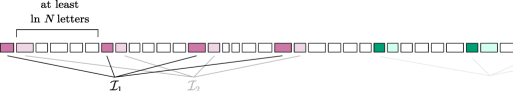
   Figure 1: A visual aid for the construction of $(\mathcal{I}_{s})_{s=1}^{s_{c}}$. Here, we imagine that $N^{r}=4$ so that $\mathcal{I}_{1}$ contains 4 indices: $i=1$, $i=7$, $i=13$ and $i=19$.

   First,

   $$\mathcal{I}_{1} =\{1,1+\ell_{-}^{-1}\ln N,1+2\ell_{-}^{-1}\ln N,\dotsc,1+(N^{r}-1)\ell_{-}^{-1}\ln N\},$$

   $$\mathcal{I}_{2} =\{2,2+\ell_{-}^{-1}\ln N,2+2\ell_{-}^{-1}\ln N,\dotsc,2+(N^{r}-1)\ell_{-}^{-1}\ln N\},$$

   $$\hskip 5.38193pt\vdots$$

   $$\mathcal{I}_{\ell_{-}^{-1}\ln N} =\{\ell_{-}^{-1}\ln N,2\ell_{-}^{-1}\ln N,3\ell_{-}^{-1}\ln N,\dotsc,N^{r}\ell_{-}^{-1}\ln N\}.$$

   Then, for as long as $(k+1)N^{r}\ell_{-}^{-1}\ln N<c$, we set

   $$\mathcal{I}_{k(\ell_{-}^{-1}\ln N)+1} =\mathcal{I}_{1}+kN^{r}\ell_{-}^{-1}\ln N,$$

   $$\mathcal{I}_{k(\ell_{-}^{-1}\ln N)+2} =\mathcal{I}_{2}+kN^{r}\ell_{-}^{-1}\ln N,$$

   $$\hskip 5.38193pt\vdots$$

   $$\mathcal{I}_{(k+1)\ell_{-}^{-1}\ln N} =\mathcal{I}_{\ell_{-}^{-1}\ln N}+kN^{r}\ell_{-}^{-1}\ln N.$$

   The two key features of these subsets are:

   • The subsets $\mathcal{I}_{1}$, $\mathcal{I}_{2},\dotsc,\mathcal{I}_{s_{c}}$ cover most of $\{1,2,\dotsc,c\}$ in the sense that

     $$\#\left(\{1,2,\dotsc,c\}\setminus\bigcup_{s=1}^{s_{c}}\mathcal{I}_{s}\right)\leq N^{r}\ell_{-}^{-1}\ln N.$$ (3.5)

     In conjunction with SE, this will allow us to neglect the contribution of $-\ln{\mathbb{P}}[\underline{w}^{(i)}]$ for $i$ not in any $\mathcal{I}_{s}$.

   • Between words $\underline{w}^{(i)}$ and  $\underline{w}^{(i^{\prime})}$ corresponding to indices $i<i^{\prime}$ in the same $\mathcal{I}_{s}$, there is a gap of at least $\ell_{-}^{-1}\ln N$ words. Provided that (3.1) holds, this amounts to a gap of at least $\ln N>\tau_{\ell_{i}}$ symbols, allowing us to make use of UD.

   Since

   $$({\mathbb{P}}\otimes{\mathbb{Q}})\left\{\sum_{i=1}^{c_{N}}-\ln{\mathbb{P}}[\underline{w}^{(i)}(y,x)]\geq(1+2\epsilon)c_{N}\ln N\right\}$$

   $$\quad\leq 2N^{-\nu}+\sum_{c=N\ell_{+}^{-1}}^{N\ell_{-}^{-1}}({\mathbb{P}}\otimes{\mathbb{Q}})\left\{\sum_{i=1}^{c}-\ln{\mathbb{P}}[\underline{w}^{(i)}(y,x)]\geq(1+2\epsilon)c\ln N,\ c_{N}=c\text{ and \eqref{eq:a-priori-bounds-a} holds}\right\}$$

   by Lemma 3.1, and since

   $$({\mathbb{P}}\otimes{\mathbb{Q}})\left\{\sum_{i=1}^{c}-\ln{\mathbb{P}}[\underline{w}^{(i)}(y,x)]\geq(1+2\epsilon)c\ln N,\ c_{N}=c\text{ and \eqref{eq:a-priori-bounds-a} holds}\right\}$$

   $$\qquad\leq({\mathbb{P}}\otimes{\mathbb{Q}})\left\{\sum_{s=1}^{s_{c}}\sum_{i\in\mathcal{I}_{s}}-\ln{\mathbb{P}}[\underline{w}^{(i)}(y,x)]\geq(1+\epsilon)c\ln N,\ c_{N}=c\text{ and \eqref{eq:a-priori-bounds-a} holds}\right\}$$

   for $N$ large enough due to (3.5) and SE, it suffices to show that for all $N$ large enough

   $$\sum_{c=N\ell_{+}^{-1}}^{N\ell_{-}^{-1}}\sum_{s=1}^{s_{c}}({\mathbb{P}}\otimes{\mathbb{Q}})(A_{c,s,(1+\epsilon)N^{r}\ln N})\leq N^{-\nu},$$ (3.6)

   where

   $$A_{c,s,t}:=\left\{(x,y):\sum_{i\in\mathcal{I}_{s}}-\ln{\mathbb{P}}[\underline{w}^{(i)}(y,x)]\geq t,\ c_{N}=c\text{ and~{}\eqref{eq:a-priori-bounds-a} holds}\right\}.$$

   This is yet another application of the Borel–Cantelli lemma.

   To this end we note that, at fixed $c$ and $s$, there are at most $N$ possibilities for the starting site of the earliest word, and then at most $\ell_{+}^{N^{r}}\cdot(\ell_{+}\cdot\ell_{-}^{-1}\ln N)^{N^{r}}=\mathrm{e}^{N^{r}O(\ln\ln N)}$ ways of choosing the lengths of the words and gaps between the words (lengths of words this group is interlaced with), provided that (3.1) holds. Therefore,

   $$({\mathbb{P}}\otimes{\mathbb{Q}})(A_{c,s,t}) \leq\mathrm{e}^{O(N^{r}\ln\ln N)}\max({\mathbb{P}}\otimes{\mathbb{Q}})\Bigg{\{}\sum_{i\in\mathcal{I}_{s}}-\ln{\mathbb{P}}[y_{L_{i-1}+1}^{L_{i-1}+l_{i}}]\geq t$$

   $$\hskip 132.0pt\text{ and }W_{l_{i}}(T^{L_{i-1}}y,x)<N\text{ for each }i\in\mathcal{I}_{s}\Bigg{\}}$$

   where the maximum is taken over choices of $(L_{i-1})_{i\in\mathcal{I}_{s}}$ and $(l_{i})_{i\in\mathcal{I}_{s}}$ satisfying the following constraints: $l_{i}\leq\ell_{+}$ for $i\in\mathcal{I}_{s}$, and $L_{i-1}+l_{i}+\ln N<L_{i^{\prime}-1}\leq L_{i-1}+l_{i}+\ell_{+}\ell_{-}^{-1}\ln N$ for consecutive $i,i^{\prime}\in\mathcal{I}_{s}$. Thanks to these constraints, we can use UD to deduce that, for any family $(B_{i})_{i\in\mathcal{I}_{s}}$ of Borel sets, we have

   $$({\mathbb{P}}\otimes{\mathbb{Q}})\left(\bigcap_{i\in\mathcal{I}_{s}}\left\{-\ln{\mathbb{P}}[y_{L_{i-1}+1}^{L_{i-1}+l_{i}}]\in B_{i}\text{ and }W_{l_{i}}(T^{L_{i-1}}y,x)<N\right\}\right)\\ \leq\mathrm{e}^{N^{r}k_{\ell_{+}}}\prod_{i\in\mathcal{I}_{s}}({\mathbb{P}}\otimes{\mathbb{Q}})\left\{-\ln{\mathbb{P}}[y_{L_{i-1}+1}^{L_{i-1}+l_{i}}]\in B_{i}\text{ and }W_{l_{i}}(T^{L_{i-1}}y,x)<N\right\}.$$ (3.7)

   Also note that, for a fixed $L$ and $l$, a union bound gives

   $$({\mathbb{P}}\otimes{\mathbb{Q}})\left\{-\ln{\mathbb{P}}[y_{L+1}^{L+l}]\geq t\text{ and }W_{l}(T^{L}y,x)<N\right\} \leq\sum_{\begin{subarray}{c}a\in\operatorname{supp}{\mathbb{P}}_{l}\\ {\mathbb{P}}[a]\leq\mathrm{e}^{-t}\end{subarray}}{\mathbb{Q}}[a]\cdot N{\mathbb{P}}[a]$$

   $$\leq N\mathrm{e}^{-t}.$$

   Hence, the Borel measure on ${\mathbb{R}}^{|\mathcal{I}_{s}|}_{+}$ uniquely specified by the left-hand side of (3.7) is bounded by a product of finite Borel measures on ${\mathbb{R}}_{+}$ that each have well-defined moment-generating functions on $(0,1)$. In Lemma A.1, we show that the same argument as in the proof of Chebyshëv’s inequality for the function $t\mapsto\mathrm{e}^{(1+\epsilon)^{-\frac{1}{2}}t}$ then implies that

   $$({\mathbb{P}}\otimes{\mathbb{Q}})(A_{c,s,t}) \leq\mathrm{e}^{O(N^{r}\ln\ln N)}\mathrm{e}^{N^{r}k_{\ell_{+}}}\mathrm{e}^{-(1+\epsilon)^{-\frac{1}{2}}t}\prod_{i\in\mathcal{I}_{s}}\frac{N}{1-(1+\epsilon)^{-\frac{1}{2}}}$$

   $$\leq\exp\left(-(1+\epsilon)^{-\frac{1}{2}}t+N^{r}\ln N+N^{r}o(\ln N)+N^{r}O(\ln\ln N)\right).$$

   With $t=(1+\epsilon)N^{r}\ln N$ and $N$ large, we find

   $$({\mathbb{P}}\otimes{\mathbb{Q}})(A_{c,s,(1+\epsilon)N^{r}\ln N}) \leq\exp\left((1+o(1)-(1+\epsilon)^{\frac{1}{2}})N^{r}\ln N+N^{r}O(\ln\ln N)\right)\leq N^{-\nu-2},$$

   implying (3.6) as desired. ∎

3.3 Ingredients III and IV

The following proposition establishes the missing ingredients for the proof of Theorem 2.5.

Proposition 3.7.

Suppose that the assumptions of Theorem 3.6 hold. Then, almost surely,

$$\liminf_{N\to\infty}\frac{1}{N-c_{N}}\sum_{i=1}^{c_{N}}-\ln{\mathbb{P}}[\underline{w}^{(i,N)}]\geq D_{-}\bar{q}(0)$$

and

$$\limsup_{N\to\infty}\frac{1}{N}\sum_{i=1}^{c_{N}-1}-\ln{\mathbb{P}}[\overline{w}^{(i,N)}]\leq D_{+}\bar{q}(0).$$

Proof.

Let $\epsilon>0$ be arbitrary. We use freely the notation from the proof of Theorem 3.6. By Lemma 3.1, almost surely, the lengths $\underline{\ell}_{i}:=|\underline{w}^{(i)}|$ are eventually all bounded below by $\ell_{-}$, except possibly for $i=c_{N}$. However, for any given value $c$ of $c_{N}(y|x)$, the index $i=c$ is not in any of the $(\mathcal{I}_{s})_{s=1}^{s_{c}}$ and so we have $\ell_{i}\geq\ell_{-}$ for each $i\in\mathcal{I}_{s}$.

Fix $c$, $s\leq s_{c}$, $(L_{i-1})_{i\in\mathcal{I}_{s}}$ and $(l_{i})_{i\in\mathcal{I}_{s}}$ with the same constraints as in the proof of Theorem 3.6.ii. If $D_{-}\bar{q}(0)<\infty$, then Markov’s inequality and UD give that, for $\alpha<0$,

$${\mathbb{Q}}\left\{y:\sum_{i\in\mathcal{I}_{s}}-\ln{\mathbb{P}}[y_{L_{i-1}+1}^{L_{i-1}+l_{i}}]\leq\sum_{i\in\mathcal{I}_{s}}l_{i}(D_{-}\bar{q}(0)-\epsilon)\right\}$$

$$\qquad\qquad\leq\mathrm{e}^{-\alpha\sum_{i\in\mathcal{I}_{s}}l_{i}(D_{-}\bar{q}(0)-\epsilon)}\mathbb{E}_{{\mathbb{Q}}}\left[\mathrm{e}^{\alpha\sum_{i\in\mathcal{I}_{s}}[-\ln{\mathbb{P}}[y_{L_{i-1}+1}^{L_{i-1}+l_{i}}]]}\right]$$

$$\qquad\qquad\leq\prod_{i\in\mathcal{I}_{s}}\mathrm{e}^{l_{i}\left[\frac{q_{l_{i}}(\alpha)}{l_{i}}-\alpha(D_{-}\bar{q}(0)-\epsilon)\right]+k_{l_{i}}}.$$

If on the contrary $D_{-}\bar{q}(0)=\infty$, then one simply substitutes “$D_{-}\bar{q}(0)-\epsilon$” with “$\epsilon^{-1}$” everywhere — we will not entertain this distinction any longer. By convexity, we may pick $\alpha<0$ small enough that

$$\bar{q}(\alpha)<\alpha\left(D_{-}\bar{q}(0)-\frac{1}{2}\epsilon\right);$$

see Figure 2.

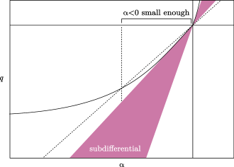
Figure 2: The dashed line has a slope that is slightly less steep than the least steep slope $D_{-}\bar{q}(0)$ in the subdifferential of the convex function $\bar{q}$ at the origin, so we can find a small region to the left of the origin where the graph of $\bar{q}$ lies below it.

Now, pick $N$ large enough that each $l_{i}\geq\ell_{-}$ for $i\in\mathcal{I}_{s}$ is guaranteed to make

$$\frac{q_{l_{i}}(\alpha)}{l_{i}}<\bar{q}(\alpha)-\frac{\alpha\epsilon}{2}$$

and

$$k_{l_{i}}\leq l_{i}\left(\alpha\left(D_{-}\bar{q}(0)-\frac{1}{2}\epsilon\right)-\bar{q}(\alpha)\right).$$

Then,

$${\mathbb{Q}}\left\{y:\sum_{i\in\mathcal{I}_{s}}-\ln{\mathbb{P}}[y_{L_{i-1}+1}^{L_{i-1}+l_{i}}]\leq\sum_{i\in\mathcal{I}_{s}}l_{i}(D_{-}\bar{q}(0)-\epsilon)\right\} \leq\mathrm{e}^{-\delta\left(\sum_{i\in\mathcal{I}_{s}}l_{i}\right)}$$

for some $\delta>0$ that does not depend on $N$.

Now, taking into account the number of choices for $(L_{i-1})_{i\in\mathcal{I}_{s}}$ and $(l_{i})_{i\in\mathcal{I}_{s}}$, we deduce that

$$({\mathbb{P}}\otimes{\mathbb{Q}})\left\{(x,y):\sum_{i\in\mathcal{I}_{s}}-\ln{\mathbb{P}}[\underline{w}^{(i)}]\leq\sum_{i\in\mathcal{I}_{s}}\underline{\ell}_{i}(D_{-}\bar{q}(0)-\epsilon)\text{ and \eqref{eq:a-priori-bounds-a} holds}\right\} \leq\mathrm{e}^{O(N^{r}\ln\ln N)}\mathrm{e}^{-\delta N^{r}\ell_{-}}$$

for every choice of $c$ and $s\leq s_{c}$. But still as in the proof of Theorem 3.6.ii, we have

$$({\mathbb{P}}\otimes{\mathbb{Q}})\left\{\sum_{i=1}^{c_{N}}-\ln{\mathbb{P}}[\underline{w}^{(i)}(y,x)]\leq\sum_{i=1}^{c_{N}}\underline{\ell}_{i}(D_{-}\bar{q}(0)-2\epsilon)\right\}$$

$$\quad\leq 2N^{-\nu}+\sum_{c=N\ell_{+}^{-1}}^{N\ell_{-}^{-1}}({\mathbb{P}}\otimes{\mathbb{Q}})\left\{\sum_{i=1}^{c}-\ln{\mathbb{P}}[\underline{w}^{(i)}(y,x)]\leq\sum_{i=1}^{c}\underline{\ell}_{i}(D_{-}\bar{q}(0)-2\epsilon),\text{ $c_{N}=c$}\text{ and \eqref{eq:a-priori-bounds-a} holds}\right\}$$

$$\quad\leq 2N^{-\nu}+\sum_{c=N\ell_{+}^{-1}}^{N\ell_{-}^{-1}}\sum_{s=1}^{s_{c}}({\mathbb{P}}\otimes{\mathbb{Q}})\left\{\sum_{i\in\mathcal{I}_{s}}-\ln{\mathbb{P}}[\underline{w}^{(i)}(y,x)]\leq\sum_{i\in\mathcal{I}_{s}}\underline{\ell}_{i}(D_{-}\bar{q}(0)-\epsilon)\text{ and \eqref{eq:a-priori-bounds-a} holds}\right\}$$

for all $N$ large enough, and conclude that we can use the Borel–Cantelli to obtain the first desired almost sure bound. The second bound is proved similarly, replacing $\underline{w}$ with $\overline{w}$, $\underline{\ell}$ with $\ell$, $D_{-}\bar{q}(0)$ with $D_{+}\bar{q}(0)$, $\alpha<0$ with $\alpha>0$, and $-\epsilon$ with $\epsilon$. ∎

3.4 A Property of the left derivative

As already mentioned at the beginning of the section, Theorem 3.6 and Proposition 3.7 imply Theorem 2.5, and Corollary 2.8 follows. Before we change point of view on the problem, we mention an important technical ingredient in the form of a theorem which will be useful in the important family of hidden-Markov measures in Section 5.1.

Theorem 3.8.

Suppose that ${\mathbb{P}}$ satisfies UD. If, in addition, ${\mathbb{Q}}$ is ergodic and satisfies UD with $\tau_{n}=O(1)$ and $k_{n}=O(1)$, then

$$D_{-}q(0)=h_{\textnormal{c}}({\mathbb{Q}}|{\mathbb{P}}).$$

Proof sketch..

Recall that the limit $q$ exists for all $\alpha\leq 0$ and has the variational expression (3.2) by Lemma 3.5. By gapped versions of Fekete’s lemma and Kingman’s theorem, one can write the maps $\mu\mapsto\alpha\int h_{\mathbb{P}}\mathop{\mathrm{\mathstrut d}}\nolimits\!\mu$ and $\mu\mapsto-\int h_{\mathbb{Q}}\mathop{\mathrm{\mathstrut d}}\nolimits\!\mu$ as infima of families of continuous maps on the space of shift-invariant Borel measures on ${\cal A}^{\mathbb{N}}$ equipped with the topology of weak convergence. Hence, these two maps are upper semicontinuous. It is also possible to show that they are affine. Both these properties are well known for the Kolmogorov–Sinai entropy map $\mu\mapsto\int h_{\mu}\mathop{\mathrm{\mathstrut d}}\nolimits\!\mu$ on shift spaces. In particular, the set of maximizers is nonempty and convex.

We follow the same strategy as for the analogous result in [BJPP18, §4.1]. Using elementary properties of convex functions and this variational expression, one can show that

$$D_{-}q(0) =\sup_{\alpha<0}\frac{q(\alpha)}{\alpha}$$

$$\leq\int h_{\mathbb{P}}\mathop{\mathrm{\mathstrut d}}\nolimits\!{\mathbb{Q}}.$$

Note that the right-hand side is the desired specific cross entropy by Lemma 3.4. If $D_{-}q(0)=\infty$, then the theorem is already established. So, we will assume otherwise for the remainder of the proof.

Consider now a sequence of maximizers $\mu(\alpha_{k})$ for (3.2) with $\alpha=\alpha_{k}$ such that $\alpha_{k}$ increases to 0 as $k\to\infty$, avoiding the points of discontinuity of $q^{\prime}$. Up to extracting a subsequence, we may assume that $\mu(\alpha_{k})$ converges weakly to some shift-invariant $\mu(0)$. Using upper semicontinuity of the aforementioned maps and the continuity of $q$ on $(-\infty,0]$, one can show that this $\mu(0)$ is a maximizer for (3.2) with $\alpha=0$. Again using upper semicontinuity one can then show that

$$D_{-}q(0) \geq\lim_{k\to\infty}\int h_{\mathbb{P}}\mathop{\mathrm{\mathstrut d}}\nolimits\!\mu(\alpha_{k})$$

$$\geq\inf_{\mu\text{ 0-eq}}\int h_{\mathbb{P}}\mathop{\mathrm{\mathstrut d}}\nolimits\!\mu,$$

where the infimum is taken over all $\mu$ in the set of maximizers for (3.2) with $\alpha=0$. Hence, the theorem will be proved if we can show that ${\mathbb{Q}}$ is the unique maximizer for (3.2) with $\alpha=0$. This can again be done following the proof of the analogous result in [BJPP18, §4.1], which is in turn along the lines of classical arguments of Ruelle summarized e.g. in [Sim, §III.8]. We will only sketch the strategy.

Let $\mu$ be any such maximizer, i.e. a shift-invariant measure such that

$$0=q(0)=-\int[h_{\mathbb{Q}}-h_{\mu}]\mathop{\mathrm{\mathstrut d}}\nolimits\!\mu.$$ (3.8)

By UD for ${\mathbb{Q}}$,

$$F_{n}:=\int[\ln{\mathbb{Q}}_{n}-\ln\mu_{n}]\mathop{\mathrm{\mathstrut d}}\nolimits\!\mu$$

defines a gapped, subadditive sequence in the sense that

$$F_{n+\tau_{n}+m} =\int[\ln{\mathbb{Q}}_{n+\tau_{n}+m}-\ln\mu_{n+\tau_{n}+m}]\mathop{\mathrm{\mathstrut d}}\nolimits\!\mu$$

$$=\sum_{a\in{\cal A}^{n}}\sum_{\xi\in{\cal A}^{\tau_{n}}}\sum_{b\in{\cal A}^{m}}\ln{\mathbb{Q}}[a\xi b]\ \mu[a\xi b]+\sum_{a\in{\cal A}^{n}}\sum_{\xi\in{\cal A}^{\tau_{n}}}\sum_{b\in{\cal A}^{m}}-\ln\mu[a\xi b]\ \mu[a\xi b]$$

$$\leq k_{n}+\sum_{a\in{\cal A}^{n}}\ln{\mathbb{Q}}[a]\ \mu[a]+\sum_{b\in{\cal A}^{m}}\ln{\mathbb{Q}}[b]\ \mu[b]$$

$$\qquad\qquad{}+\sum_{a\in{\cal A}^{n}}-\ln\mu[a]\ \mu[a]+\sum_{\xi\in{\cal A}^{\tau_{n}}}-\ln\mu[\xi]\ \mu[\xi]+\sum_{b\in{\cal A}^{m}}-\ln\mu[b]\ \mu[b]$$

$$\leq k_{n}+F_{n}+F_{m}+\tau_{n}\ln(\#A).$$

For the triple sum involving $\mu$ only, we have used subadditivity of entropy for measures on products of finite sets. By combining gapped versions of Fekete’s lemma and Kingman’s theorem [Raq23, §§II–III] with the Shannon–McMillan–Breiman theorem, we then have

$$\int[h_{\mathbb{Q}}-h_{\mu}]\mathop{\mathrm{\mathstrut d}}\nolimits\!\mu=\inf_{n\in{\mathbb{N}}}\frac{F_{n}+k_{n}+\tau_{n}\ln(\#A)}{n+\tau_{n}}.$$ (3.9)

Combining (3.8) and (3.9), we deduce that

$$0\leq-F_{n}\leq k_{n}+\tau_{n}\ln(\#A).$$

for all $n\in{\mathbb{N}}$. Reinterpreting $-F_{n}$ as the — not specific — relative entropy of the $n$-th marginal of $\mu$ with respect to the $n$-th marginal of ${\mathbb{Q}}$, we deduce that $k_{n}+\tau_{n}\ln(\#A)$ being $O(1)$ implies $\mu\ll{\mathbb{Q}}$. But if ${\mathbb{Q}}$ is ergodic, then this in turn implies that $\mu={\mathbb{Q}}$. ∎

4 A Rigidity problem

Once Proposition 3.6 has established Ingredients I and II, one can change point of view and focus on the “rigidity” of Lemma 3.4. Here, “rigidity” of the result is to be understood in the sense of the following problem on what happens to the convergence in this lemma as we cut $y_{1}^{N}$ into (mostly) moderately long words.

Problem.

Suppose $(\ell_{i,N})_{i=1}^{c_{N}}$ and $(\mu_{i,N})_{i=0}^{c_{N}}$ are nonnegative, integer-valued random variables satisfying

$$C^{-1}(\ln N)^{\frac{1}{C}}\leq\ell_{i,N}\leq C\ln N$$

for some $C\geq 1$, as well as

$$\sum_{i=1}^{c_{N}}\ell_{i,N}=N-o(N)\qquad\text{and}\qquad\sum_{i=0}^{c_{N}}\mu_{i,N}=o(N).$$

Let

$$L_{i,N}:=\sum_{i^{\prime}=0}^{i}\mu_{i^{\prime},N}+\sum_{i^{\prime}=1}^{i}\ell_{i^{\prime},N}.$$

What is a “natural” class of pairs $({\mathbb{P}},{\mathbb{Q}})$ of measures with ${\mathbb{P}}$ satisfying UD that guarantees that

$$\lim_{N\to\infty}\frac{-\sum_{i=1}^{c_{N}}\ln{\mathbb{P}}\left[y_{L_{i-1,N}+1}^{L_{i-1,N}+\ell_{i,N}}\right]}{\sum_{i=1}^{c_{N}}\ell_{i,N}}=h_{\textnormal{c}}({\mathbb{Q}}|{\mathbb{P}})$$

for ${\mathbb{Q}}$-almost every $y$ when ${\mathbb{Q}}$ is ergodic?

One of the difficulties faced in tackling this problem is that Lemma 3.4 itself comes with no concrete estimate and that a naive large-deviation approach — which is implicitly behind Proposition 3.7 — fails to distinguish between $h_{\textnormal{c}}({\mathbb{Q}}|{\mathbb{P}})$ and other points that could be in the subdifferential of the pressure at the origin. In some sense, an answer to this problem would only be satisfactory if it at least allowed one to recover the special cases that we are about to discuss over the course of the lemmas below. And ideally, the proof techniques would be unified.

We first show that partial results regarding this open problem — in conjunction with Lemma 3.1, Theorem 3.6 and Lemma 3.4 — provide improvements over (2.4a) or (2.4b) without differentiability. For our first lemma, the improvement is perhaps most interesting when further combined with Theorem 3.8, as in Section 5.1; see Corollary 4.4.

Lemma 4.1.

If ${\mathbb{P}}$ satisfies UD with $\tau_{n}=0$ for all $n$, and $y_{1}^{N}$ is parsed according to the mZM parsing, then

$$-\sum_{i=1}^{c_{N}-1}\ln{\mathbb{P}}[\overline{w}^{(i,N)}]\leq-\ln{\mathbb{P}}[y_{1}^{N}]+o(N)$$

on the set where $|\overline{w}^{(i,N)}|\geq\ell_{-,N}$ for each $i=1,2,\dotsc,c_{N}-1$.

Proof.

The upper-decoupling assumption immediately gives

$$\ln{\mathbb{P}}[y_{1}^{N}] \leq\ln{\mathbb{P}}[y_{1}^{N-\ell_{c_{N}}}]\leq\sum_{i=1}^{c_{N}-2}k_{\ell_{i}}+\sum_{i=1}^{c_{N}-1}\ln{\mathbb{P}}[\overline{w}^{(i)}].$$

To conclude, we use that $\sum_{i=1}^{c_{N}-2}\ell_{i}<N$, that $k_{\ell}=o(\ell)$ and that ${\ell_{i}}\geq\ell_{-}$. ∎

Remark 4.2.

By a very similar argument, the conclusion still holds if one replaces the requirement that $\tau_{n}=0$ with $\tau_{n}=O(1)$ and the following lower-bound:

$$\inf\left\{\frac{{\mathbb{P}}[ab]}{{\mathbb{P}}[a]}:a\in\operatorname{supp}{\mathbb{P}}_{n},b\in\operatorname{supp}{\mathbb{P}}_{1},ab\in\operatorname{supp}{\mathbb{P}}_{n+1}\right\}\geq\mathrm{e}^{-k_{n}}$$ (4.1)

for every $n\in{\mathbb{N}}$. While such a lower bound is immediate if the measure ${\mathbb{P}}$ satisfies the weak Gibbs condition given below, it could fail for some important examples in which $\tau_{n}=0$.

Remark 4.3.

Note that the proof makes no use of the particularities of the mZM parsing; it relies solely on the fact that $y_{1}^{N}$ is parsed into words whose lengths have a lower bound that diverges as $N\to\infty$. A similar remark applies to Lemmas 4.5 and 4.7, where we use the fact that the lengths have a lower bound that grows like a power of a logarithm.

Corollary 4.4.

If, in addition to the hypotheses of Theorem 2.5, the measure ${\mathbb{P}}$ satisfies UD with $\tau_{n}=0$ for all $n$ and ${\mathbb{Q}}$ is ergodic, then

$$D_{-}\overline{q}(0) \leq\liminf_{N\to\infty}Q_{N}(y,x)$$ (4.2a)

$$\leq\limsup_{N\to\infty}Q_{N}(y,x)\leq h_{\textnormal{c}}({\mathbb{Q}}|{\mathbb{P}})$$ (4.2b)

for $({\mathbb{P}}\otimes{\mathbb{Q}})$-almost every $(x,y)$. If, moreover, ${\mathbb{Q}}$ satisfies UD with $\tau_{n}=O(1)$ and $k_{n}=O(1)$, then

$$\lim_{N\to\infty}Q_{N}(y,x)=h_{\textnormal{c}}({\mathbb{Q}}|{\mathbb{P}})$$ (4.3)

for $({\mathbb{P}}\otimes{\mathbb{Q}})$-almost every $(x,y)$.

Our second partial result concerns the weak Gibbs (WG) class of Yuri on a subshift $\Omega^{\prime}\subseteq{\cal A}^{\mathbb{N}}$, i.e. the class of measures ${\mathbb{P}}$ for which there exists a continuous function $\phi:\Omega^{\prime}\to{\mathbb{R}}$ and a nondecreasing $\mathrm{e}^{o(n)}$-sequence $(K_{n})_{n=1}^{\infty}$ such that

$$K_{n}^{-1}\mathrm{e}^{\sum_{j=0}^{n-1}\phi(T^{j}y)-np_{\textnormal{top}}(\phi)}\leq{\mathbb{P}}[y_{1}^{n}]\leq K_{n}\mathrm{e}^{\sum_{j=0}^{n-1}\phi(T^{j}y)-np_{\textnormal{top}}(\phi)}$$

for every $y\in\Omega^{\prime}$. Here, $p_{\textnormal{top}}(\phi)$, known as the topological pressure, is completely determined by $\phi$, and provides the appropriate normalization. On subshifts with suitable specification properties, $g$-measures and equilibrium measures for absolutely summable interactions are WG; we do not dwell on this technical issue and instead refer the reader to [PS20]. The next lemma — in conjunction with Lemmas 3.1 and 3.4 and Theorem 3.6 — shows again that progress on this open problem can be beneficial.

Lemma 4.5.

If ${\mathbb{P}}$ is WG and $y_{1}^{N}$ is parsed according to the mZM parsing, then

$$-\ln{\mathbb{P}}[y_{1}^{N}]-o(N)\leq-\sum_{i=1}^{c_{N}}\ln{\mathbb{P}}[\underline{w}^{(i,N)}]$$

and

$$-\sum_{i=1}^{c_{N}-1}\ln{\mathbb{P}}[\overline{w}^{(i,N)}]\leq-\ln{\mathbb{P}}[y_{1}^{N}]+o(N).$$

on the set where $|\overline{w}^{(i,N)}|\geq\ell_{-,N}$ for each $i=1,2,\dotsc,c_{N}-1$.

Proof.

Without loss of generality, we assume that $p_{\textnormal{top}}(\phi)=0$. Both bounds are proved similarly so we only provide the proof of the first one. With any $y\in[y_{1}^{N}]$, we have by WG that

$$\ln{\mathbb{P}}[y_{1}^{N}] \geq-\ln K_{N}+\sum_{j=0}^{N-1}\phi(T^{j}y)$$

$$=-\ln K_{N}+\sum_{i=1}^{c_{N}}\sum_{j=L_{i-1}}^{L_{i-1}+\ell_{i}-1}\phi(T^{j}y)$$

$$\geq-\ln K_{N}+\sum_{i=1}^{c_{N}}\left[\sum_{j=L_{i-1}}^{L_{i-1}+\ell_{i}-2}\phi(T^{j}y)-\|\phi\|_{\infty}\right]$$

$$\geq-\ln K_{N}-c_{N}\|\phi\|_{\infty}-\sum_{i=1}^{c_{N}}\ln K_{\ell_{i}}+\sum_{i=1}^{c_{N}}\ln{\mathbb{P}}[\underline{w}^{(i)}].$$

To conclude, we use that $\sum_{i=1}^{c_{N}}\ell_{i}=N$, that $\ln K_{\ell}=o(\ell)$ and that ${\ell_{i}}\geq\ell_{-}$. ∎

Corollary 4.6.

If, in addition to the hypotheses of Theorem 2.5, the measure ${\mathbb{P}}$ has the WG property and ${\mathbb{Q}}$ is ergodic, then

$$\lim_{N\to\infty}Q_{N}(y,x)=h_{\textnormal{c}}({\mathbb{Q}}|{\mathbb{P}})$$

for $({\mathbb{P}}\otimes{\mathbb{Q}})$-almost every $(x,y)$.

Our last technical result deals with the case of a lower-decoupling condition related to SLD.

CLD

A measure is said to satisfy the common-word lower-decoupling condition if there exists a $o(n)$-sequence $(k_{n})_{n=1}^{\infty}$, an $L\in{\mathbb{N}}$ and some word ${\mathfrak{c}}\in{\cal A}^{L}$ with the following property: for all $n\in{\mathbb{N}}$, $a\in\operatorname{supp}{\mathbb{P}}_{n}$, $m\in{\mathbb{N}}$ and $b\in\operatorname{supp}{\mathbb{P}}_{m}$ with $a{\mathfrak{c}}b\in\operatorname{supp}{\mathbb{P}}_{n+L+m}$, we have

$${\mathbb{P}}[a{\mathfrak{c}}b]\geq\mathrm{e}^{-k_{n}}{\mathbb{P}}[a]{\mathbb{P}}[b].$$ (4.4)

Lemma 4.7.

Suppose that ${\mathbb{P}}$ satisfies SE and that ${\mathbb{Q}}$ satisfies UD and SLD. If, in addition, ${\mathbb{P}}$ satisfies CLD with ${\mathfrak{c}}\in\operatorname{supp}{\mathbb{Q}}$, then

$$-\sum_{i=1}^{c_{N}}\ln{\mathbb{P}}[\underline{w}^{(i,N)}]\geq-\ln{\mathbb{P}}[y_{1}^{N}]-o(N)$$

for ${\mathbb{Q}}$-almost every $y$.

Proof sketch.

Unfortunately, the proof of this lemma is quite technical and for this reason is differed to the appendix. We provide here the basic idea behind the proof. Let $L_{N}$ be a very slowly diverging sequence of natural numbers, and suppose that, for each $i$, the common word ${\mathfrak{c}}$ were to appear between the $L_{N}$-th and $2L_{N}$-th letter of $\overline{w}^{(i)}$, and similarly near the end of $\overline{w}^{(i)}$. Then, we would have

$$y_{1}^{N}=\xi^{(1)}{\mathfrak{c}}\underline{\underline{w}}^{(1)}{\mathfrak{c}}\xi^{(2)}{\mathfrak{c}}\underline{\underline{w}}^{(2)}\dotsc{\mathfrak{c}}\underline{\underline{w}}^{(c_{N})}{\mathfrak{c}}\xi^{(c_{N}+1)}$$

for some substrings $\underline{\underline{w}}^{(i)}$ of $\underline{w}^{(i)}$ and some buffers $\xi^{(i)}$ with comparatively small, yet diverging lengths. In particular, thanks to SE, $\ln{\mathbb{P}}[\xi^{(i)}]$ is not too negative. We could then use CLD repeatedly and the behaviour of the decoupling constants $k_{n}=o(n)$ to deduce that

$$\ln{\mathbb{P}}[y_{1}^{N}] \geq\ln{\mathbb{P}}[\xi^{(1)}]-k_{|\xi^{(1)}|}+\ln{\mathbb{P}}[\underline{\underline{w}}^{(1)}]-k_{|\underline{\underline{w}}^{(1)}|}+\ln{\mathbb{P}}[\xi^{(2)}]-k_{|\xi^{(2)}|}+\ln{\mathbb{P}}[\underline{\underline{w}}^{(2)}]$$

$$\hskip 144.54pt+\dotsb+\ln{\mathbb{P}}[\underline{\underline{w}}^{(c_{N})}]-k_{|\underline{\underline{w}}^{(c_{N})}|}+\ln{\mathbb{P}}[\xi^{(c_{N}+1)}]$$

$$=\sum_{i=1}^{c_{N}}\ln{\mathbb{P}}[\underline{\underline{w}}^{(i)}]-o(N).$$

Unfortunately, such a scenario is too much to ask for, but we will show in Appendix A.1 that, ${\mathbb{Q}}$-almost surely, there exists a subset $\mathcal{I}\subseteq\{1,\dotsc,c_{N}\}$ and corresponding strict substrings $\underline{\underline{w}}^{(i)}$ of $\underline{w}^{(i)}$ such that

$$\ln{\mathbb{P}}[y_{1}^{N}]\geq\sum_{i\in\mathcal{I}}\ln{\mathbb{P}}[\underline{\underline{w}}^{(i)}]-o(N),$$

which implies the desired bound. ∎

Corollary 4.8.

If, in addition to the hypotheses of Theorem 2.5, the measures ${\mathbb{P}}$ and ${\mathbb{Q}}$ satisfy the hypotheses of Lemma 4.7 and ${\mathbb{Q}}$ is ergodic, then

$$\lim_{N\to\infty}Q_{N}(y,x)=h_{\textnormal{c}}({\mathbb{Q}}|{\mathbb{P}})$$

for $({\mathbb{P}}\otimes{\mathbb{Q}})$-almost every $(x,y)$.

Although this result is technical and requires strengthening the lower-decoupling assumptions, it provides the final assertion of Corollary 4.4 under a weaker upper-decoupling assumption on ${\mathbb{Q}}$. More precisely, it circumvents the need for the upper-decoupling constants $k_{n}$ of the measure ${\mathbb{Q}}$ to be bounded at the cost of assuming both SLD on ${\mathbb{Q}}$ and CLD on ${\mathbb{P}}$. While condition CLD is not quite satisfactory in terms of its breath of applicability in the decoupling framework, Corollary 4.8 bears hope for a more general result only in terms of SLD, UD and mild decay assumptions. Importantly, Corollary 4.8 shows that although the final assertion of Corollary 4.4 encompasses a great deal of important examples, it fails to capture some classes of measures for which the almost sure convergence still holds; see Section 5.2.

5 Examples

5.1 Hidden-Markov measures with finite hidden alphabets

A shortcoming of previous rigorous works on the Ziv–Merhav theorem is that measures arising from hidden-Markov models — which we are about to properly define — were not covered at a satisfying level of generality. This shortcoming is significant since hidden-Markov models are becoming increasingly popular in applications and simulations, and can display very interesting properties from a mathematical point of view. In [BGPR23, §4.4], we were essentially only able to treat them under conditions [CU03, Yoo10] that guaranteed the g-measure property.

We call ${\mathbb{P}}$ a stationary hidden-Markov measure (HMM) if it can be represented by a tuple $(\pi,P,R)$ where $(\pi,P)$ is a stationary Markov chain on a countable set $\mathcal{S}$, $R$ is a $(\#\mathcal{S})$-by-$(\#{\cal A})$ matrix whose rows each sum to 1, and

$${\mathbb{P}}[a_{1}^{n}]=\sum_{s_{1}^{n}\in\mathcal{S}^{n}}\pi_{s_{1}}R_{s_{1},a_{1}}P_{s_{1},s_{2}}R_{s_{2},a_{2}}\cdots P_{s_{n-1},s_{n}}R_{s_{n},a_{n}}$$

for $n\in{\mathbb{N}}$ and $a_{1}^{n}\in{\cal A}^{n}$. One particular case of interest is when the matrix $R$ contains only $0$s and $1$s, in which case we often speak of a function-Markov measure. In this subsection, we restrict our attention to the case where $\mathcal{S}$ is finite.

In [BCJP21, §2.2], it is shown that the class of stationary HMMs coincides with the class of stationary positive-matrix-product measures (PMP), which are defined by a tuple $(\pi,\{M_{a}\}_{a\in{\cal A}})$ where $(\pi,M)$ is a stationary Markov measure on $\Omega$ with $M:=\sum_{a\in{\cal A}}M_{a}$ and

$${\mathbb{P}}[a_{1}^{n}]=\braket{\pi,M_{a_{1}}\cdots M_{a_{n}}\mathbbm{1}}.$$

From now on, we only consider HMMs which admit a representation with an irreducible chain $(\pi,P)$.

Expressed in terms of $(\pi,P,R)$, it easy to see how one can sample sequences from such a measure — this is much more straightforward than for the measures of Section 5.3 — in order to perform numerical experiments. This allows us to compare the performance of the mZM estimator to the longest-match estimator, whose consistency has been established more generally [Kon98, CDEJR23]; see Figure 3.

Expressed in terms of $(\pi,\{M_{a}\}_{a\in{\cal A}})$, some of the decoupling properties of an irreducible HMM are more transparent:

• Condition UD holds with $\tau_{n}=0$ and $k_{n}=O(1)$;

• Condition SLD holds with $\tau_{n}=O(1)$ and $k_{n}=O(1)$;

• Condition SE holds with $\beta=1$;

• Ergodicity holds;

• A mild condition for ND (via Remark 2.4) was provided in [BGPR23, §4.4].

Therefore, the second part of Corollary 4.4 applies for pairs of irreducible HMMs with ND, and almost sure convergence to $h_{\textnormal{c}}({\mathbb{Q}}|{\mathbb{P}})$ holds, as in the case of a differentiable pressure at the origin, even if to the best of our knowledge, the differentiability of the cross-entropic pressure $q$ at the origin for a pair of HMMs with finite hidden alphabet remains unknown. It is known that not all HMMs satisfy the WG property; see e.g. [BCJP21, §2.1.2], so almost sure convergence certainly cannot be derived from Corollary 4.6.

There is another important family of measures that shares most of these decoupling properties. Letting $\mathcal{H}$ denote a finite-dimensional Hilbert space, and $\mathcal{B}(\mathcal{H})$, the space of linear operators on $\mathcal{H}$, with identity by $\mathbbm{1}$, consider a quantum measurement described by completely positive maps $(\Phi_{a})_{a\in\mathcal{A}}$ on $\mathcal{B}(\mathcal{H})$ and a faithful initial state $\rho$ such that $\Phi:=\sum_{a\in\mathcal{A}}\Phi_{a}$ satisfies $\Phi[\mathbbm{1}]=\mathbbm{1}$ and $\rho\circ\Phi=\rho$. As usual, ${\cal A}$ is assumed to be a finite set. The unraveling of $(\rho,(\Phi_{a})_{a\in\mathcal{A}})$ is a shift-invariant measure ${\mathbb{P}}$ on $\mathcal{A}^{{\mathbb{N}}}$ defined by the marginals

$${\mathbb{P}}[a_{1}a_{2}\dots a_{n}]:=\textnormal{tr}(\rho(\Phi_{a_{1}}\circ\dots\circ\Phi_{a_{n}})[\mathbbm{1}]).$$

In the case where the completely positive map $\Phi$ is irreducible, then, similar to irreducible HMMs, we have

• Condition UD holds with $\tau_{n}=0$ and $k_{n}=O(1)$;

• Condition SLD holds with $\tau_{n}=O(1)$ and $k_{n}=O(1)$;

• Ergodicity holds;

see [BCJP21, §1]. However, SE may fail, so it has to be checked on a case-by-case basis; see [BCJP21, §5]. Also, using remark 2.7, we see that ND will hold whenever the measure ${\mathbb{Q}}$ has a strictly positive entropy. Another important difference with HMMs is that, for quantum instruments, we have explicit examples of measures for which WG fails and where the cross-entropic pressure $q$ is not differentiable at the origin, showing that Corollary 4.4 does not yield results covered by either Corollary 2.8 or 4.6.

Remark 5.1.

In practice, at a given $N$, naive implementations of the mZM and ZM algorithms will be much slower than the more well-studied longest-match length estimator as one has $c_{N}\sim N/\ln N$ for $N$ large under the conditions for which $Q_{N}\to h_{\textnormal{c}}$ as $N\to\infty$. Therefore, the complexity for $Q_{N}$ can be naively thought as $O(N/\ln N)$ times that of computing $\Lambda_{N}$. However, the foremost advantage of the mZM and ZM estimators is its faster convergence in $N$, as seen in Figure 3, which yields the most practical importance in cases where data access is limited. We do not claim any significant improvement in performance going from ZM to mZM.

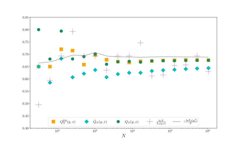
Figure 3: The convergence of various estimators to $h_{\textnormal{c}}({\mathbb{Q}}|{\mathbb{P}})$ is illustrated in a numerical experiment. Namely, $Q_{N}$ is the mZM estimator introduced herein, $\tilde{Q}_{N}$ is the mZM estimator without the $-c_{N}$ “correction” in the denominator, $Q_{N}^{\textnormal{ZM}}$ is the original ZM estimator presented in [BGPR23] and [ZM93], and $\ln N/\Lambda_{N}$ is the longest-match length estimator, which has been shown to be asymptotically consistent under weaker assumptions [Kon98, CDEJR23]. They are compared to the sequence in Lemma 3.4, which is computable here as we know the marginals of the measure ${\mathbb{P}}$, which is of course not the case in practical applications. Here, both ${\mathbb{Q}}$ and ${\mathbb{P}}$ are stationary HMMs on $\{\mathsf{0},\mathsf{1}\}^{\mathbb{N}}$.

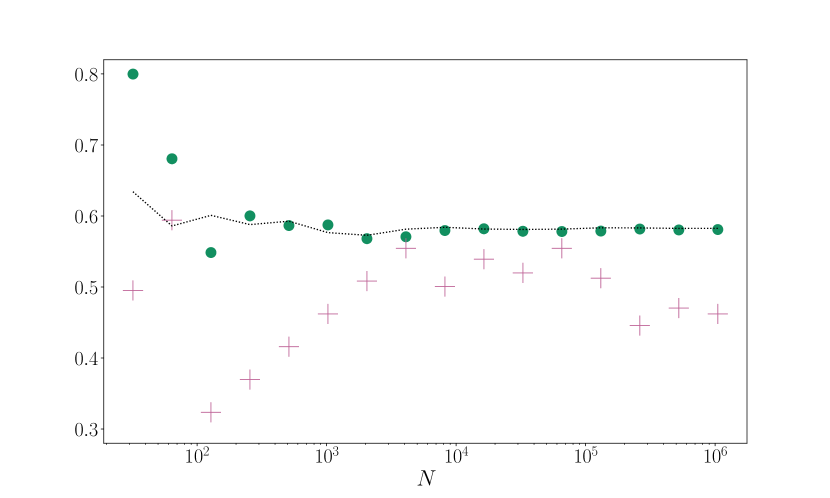
Figure 4: Both ${\mathbb{Q}}$ and ${\mathbb{P}}$ are the HMM given in Example 4.5 of [BGPR23, §4], where (4.1) does not hold.

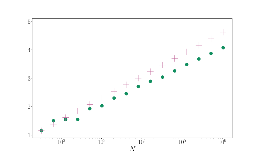
Figure 5: ${\mathbb{Q}}$ is fully supported Bernoulli measure on $\{\mathsf{0},\mathsf{1},\mathsf{2}\}^{\mathbb{N}}$ and ${\mathbb{P}}$ is a HMM on $\Omega$ with $\operatorname{supp}{\mathbb{P}}\subsetneq\{\mathsf{0},\mathsf{1},\mathsf{2}\}^{\mathbb{N}}$.

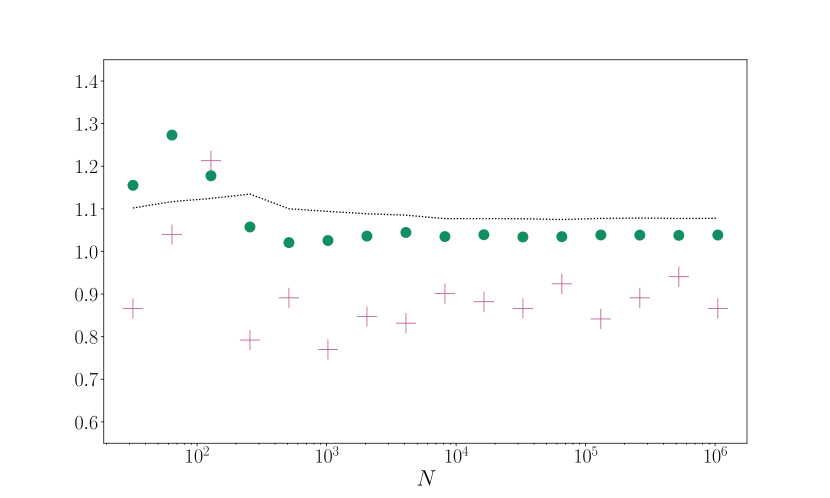
Figure 6: ${\mathbb{P}}$ is a Markov measure and ${\mathbb{Q}}$ a HMM on $\{\mathsf{0},\mathsf{1},\mathsf{2}\}^{\mathbb{N}}$.

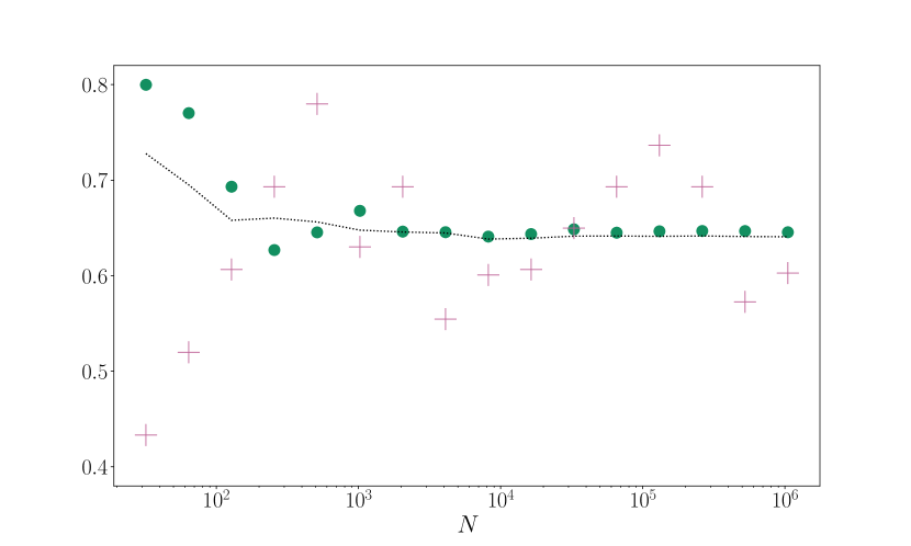
Figure 7: ${\mathbb{Q}}$ and ${\mathbb{P}}$ both come from the so-called “Keep-Switch instrument” — which belongs to the family of HMMs — with parameters $(q_{1},q_{2})=(\tfrac{1}{2},\tfrac{1}{4})$; see [BCJP21, §2.1].

5.2 Hidden-Markov measures with countably infinite hidden alphabets

In the setup of the previous subsection, if one drops the assumption that the hidden alphabet $\mathcal{S}$ is finite, then examples with irreducibility where our decoupling assumptions fail can easily be constructed. While a general understanding of this situation is out of reach, it allows us to construct interesting examples for exploring the relations between our different assumptions and results.

More precisely, there is a class of pairs of hidden-Markov measures with hidden alphabet ${\mathbb{N}}_{0}$ for which Corollary 4.8 ensures the convergence of the mZM estimator to the cross entropy, despite the fact that our analysis of the cross-entropic pressure is not sufficient to ensure the applicability of Corollary 4.4 or Corollary 2.8. The example is adapted from [CJPS19, §A.2].

Consider any nonnegative function $\gamma:{\mathbb{N}}_{0}\rightarrow{\mathbb{R}}$, with the property that $\gamma(0)=0$ and such that there exists $\epsilon>0$ so that $\gamma(n+1)\geq\gamma(n)+\epsilon$ for all $n\in{\mathbb{N}}_{0}$. Then, one can consider the stationary Markov chain on ${\mathbb{N}}_{0}$ with transition probabilities $P_{i,j}$ given by

$$P_{i,j}=\begin{cases}\mathrm{e}^{\gamma(i)-\gamma(i+1)}&\text{if }j=i+1,\\ 1-\mathrm{e}^{\gamma(i)-\gamma(i+1)}&\text{if }j=0,\\ 0&\text{otherwise};\end{cases}$$

see Figure 8. These transitions admit an invariant probability vector $\pi$; it has components of the form $\pi_{n}=Z^{-1}\mathrm{e}^{-\gamma(n)}$ for some normalization constant $Z>0$. Let ${\cal A}=\{\mathsf{a},\mathsf{b}\}$ and consider the hidden-Markov measure ${\mathbb{P}}$ on ${\cal A}^{\mathbb{N}}$ specified by $(\pi,P)$ and the matrix $R$ with elements

$$R_{s,a}=\begin{cases}1&\text{if }s=0\text{ and }a=\mathsf{a},\\ 1&\text{if }s>0\text{ and }a=\mathsf{b},\\ 0&\text{otherwise}.\end{cases}$$

This is equivalent to taking the preimage of the stationary Markov measure associated to $(\pi,P)$ under a single-site factor map that takes $0$ to $\mathsf{a}$ and every other $n$ to $\mathsf{b}$.

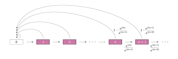
Figure 8: An illustration of the Markov chain with countably infinite alphabet used in the construction in Section 5.2.

Furthermore, if we set

$$s(n):=\sup_{m\in{\mathbb{N}}_{0}}[\gamma(n)+\gamma(m)-\gamma(n+m)],$$

then following conditions hold for ${\mathbb{P}}$:

• Condition UD holds with $\tau_{n}=0$ and $k_{n}=s(n)+O(1)$ whenever $s(n)=o(n)$;

• Condition CLD holds with ${\mathfrak{c}}=\mathsf{a}$ and $k_{n}^{\prime}=O(1)$;

• Ergodicity holds;

• Condition SE holds whenever $\gamma(n)=O(n^{\beta})$ for some $\beta\geq 1$;

• There exists $\delta>0$ such that $0<{\mathbb{P}}[x_{1}^{n}]\leq\mathrm{e}^{-\delta n}$ for all $x_{1}^{n}\in{\cal A}^{n}$ and $n\in{\mathbb{N}}$;

see [CJPS19, §A.2] for more details. The last bullet implies via Remark 2.4 that ND holds regardless of the measure ${\mathbb{Q}}$. Importantly, the choice of $k_{n}$ in the first bullet is tight in the sense that there exists some constant $c\geq 0$ so that

$$\mathrm{e}^{-c+s(n)}\leq\sup_{m\in{\mathbb{N}}_{0}}\frac{{\mathbb{P}}[\mathsf{b}^{n+m}]}{{\mathbb{P}}[\mathsf{b}^{n}]{\mathbb{P}}[\mathsf{b}^{m}]}\leq\mathrm{e}^{c+s(n)}.$$

Here, we have used the notation $\mathsf{b}^{k}$ for the symbol $\mathsf{b}$ repeated $k$ times in a row. Therefore, if $\gamma$ is chosen so that $s(n)=o(n)$ but not $O(1)$, then the above produces examples that cannot satisfy UD with $k_{n}=O(1)$. Now, taking for example

$$\gamma_{1}(n) =n^{2},$$

$$\gamma_{2}(n) =n+\ln(1+n),$$

we have

1. $s_{2}(n)=\ln(n)$ is $o(n)$ but not $O(1)$;

2. $\limsup_{n\to\infty}\frac{\alpha\gamma_{1}(n)-\gamma_{2}(n)}{n}=\infty$, for all $\alpha>0$;

3. $0<\sum_{n=1}^{\infty}\gamma_{1}(n)\mathrm{e}^{-\gamma_{2}(n)}<\infty$.

Considering the measures ${\mathbb{P}}$ and ${\mathbb{Q}}$ that are induced by $\gamma_{1}$ and $\gamma_{2}$ respectively, we have the following situation. Property ii implies that $\bar{q}(\alpha)=\infty$ for all $\alpha\in(0,\infty)$, and hence that $D_{+}\overline{q}(0)=\infty$. The significance of Property iii comes form the fact that —following the strategy of [BCJP21, §5] —one can also show that there exists a constant $C>0$ such that

$$C^{-1}\sum_{n=1}^{\infty}\gamma_{1}(n)\mathrm{e}^{-\gamma_{2}(n)}\leq h_{\textnormal{c}}({\mathbb{Q}}|{\mathbb{P}})\leq C\sum_{n=1}^{\infty}\gamma_{1}(n)\mathrm{e}^{-\gamma_{2}(n)}.$$

Hence, we have that $D_{-}\bar{q}(0)\leq h_{\textnormal{c}}({\mathbb{Q}}|{\mathbb{P}})<D_{+}\bar{q}(0)$ and $0<h_{\textnormal{c}}({\mathbb{Q}}|{\mathbb{P}})$. Therefore, thanks to Property i, Corollary 4.8 ensures the convergence of the mZM estimator to the cross entropy, while neither Corollary 4.4 nor Corollary 2.8 applies.

5.3 Statistical mechanics

In this subsection, we use a particular family of models from statistical mechanics as a mean to further illustrate the applicability of some of our results. While the decoupling and decay properties are discussed in the context of more general summable interactions in [CR23, BGPR23], we focus here on long-range ferromagnetic models on ${\mathbb{Z}}$. In this context, a translation-invariant Gibbs measure ${\mathbb{P}}$ on $\{-1,+1\}^{\mathbb{N}}$ can be obtained from a limiting procedure starting from finite-volume (volume $n$) Hamiltonians

$$H_{h,J,n}:\{-1,+1\}^{\{-n,-n+1,\dotsc,n\}} \to{\mathbb{R}}$$

$$(a_{-n},a_{-n+1},\dotsc,a_{n}) \mapsto-\sum_{i=-n}^{n}\sum_{j=i+1}^{n}J_{|j-i|}a_{i}a_{j}-h\sum_{i=-n}^{n}a_{i}$$

for each $n\in{\mathbb{N}}$, where $(J_{k})_{k=1}^{\infty}$ is a summable, positive sequence and $h$ is a real parameter (the field strength), and from an additional positive parameter $\beta$ (the inverse temperature). We do not describe this well-known procedure, which can be found e.g. in [Ell, §IV.2].

While the WG property [PS20, §2] and UD and SLD with $\tau_{n}=0$ [LPS95, §9] are guaranteed in this setup, differentiability of the pressure $q$ at the origin could fail. To see this, take ${\mathbb{Q}}$ to be a translation-invariant Gibbs measure with $J^{{\mathbb{Q}}}_{k}=k^{-\frac{3}{2}}$ and $h=0$ at $\beta>\beta_{\textnormal{c}}$, and ${\mathbb{P}}$ to be a translation-invariant Gibbs measure with $J^{{\mathbb{P}}}_{k}=0$ and $h=1$ at the same $\beta$. Then, up to a constant factor, $\alpha\mapsto q(\alpha)$ coincides with the specific free energy for $(J^{{\mathbb{Q}}}_{k})_{k=1}^{\infty}$ as a function of $h$ — keeping the same $\beta$. The latter is known not to be differentiable at $h=0$; see [Ell, §IV.5]. Because SE and ND cause no issue here [BGPR23, §4.3], this example shows that Corollary 4.6 does cover cases not covered by Corollary 2.8.

It is worth noting that for sequences $(J_{k})_{k=1}^{\infty}$ that decay fast enough, the WG property can be strengthened to the Bowen–Gibbs property (i.e. WG with $K_{n}=O(1)$), so almost sure convergence can equivalently be deduced from Corollary 2.8, 4.4 or 4.6.

Appendix A Appendix

A.1 Proof of Lemma 4.7

In this subsection of the appendix, we present the technical proof of Lemma 4.7.

Proof.

We will show that there exists a subset $\mathcal{I}\subseteq\{1,\dotsc,c_{N}\}$ and corresponding strict substrings $\underline{\underline{w}}^{(i)}$ of $\underline{w}^{(i)}$ such that

$$\ln{\mathbb{P}}[y_{1}^{N}]\geq\sum_{i\in\mathcal{I}}\ln{\mathbb{P}}[\underline{\underline{w}}^{(i)}]-o(N)$$ (A.1)

by constructing $\mathcal{I}$ in two disjoint parts, $\mathcal{I}_{\mathrm{g}}$ (“g” stands for “good”) and $\mathcal{I}_{\mathrm{l}}$ (“l” stands for “long”), with the following properties.

1. For $i\in\mathcal{I}_{\mathrm{g}}$, there are, by definition, boundary intervals $J_{1}^{(i)}$ and $J_{2}^{(i)}$ close to the edges of $\overline{w}^{(i)}$ where we can find the common word ${\mathfrak{c}}$ and decouple using CLD contributing $\ln{\mathbb{P}}[\underline{\underline{w}}^{(i)}]$ to (A.1).

2. For $i\in\mathcal{I}_{\mathrm{l}}$, we are also able to extract a contribution $\ln{\mathbb{P}}[\underline{\underline{w}}^{(i)}]$ to (A.1), based solely on the fact that $\overline{w}^{(i)}$ is long enough. The neighbouring buffers can be longer and have smaller probability, but there are not too many of them.

3. Using SE, we can show that in the presence of two consecutive $i$ in either $\mathcal{I}_{\mathrm{g}}$ or $\mathcal{I}_{\mathrm{l}}$, the contribution of the buffer $\xi^{(i)}$ between $\underline{\underline{w}}^{(i)}$ and $\underline{\underline{w}}^{(i+1)}$ is negligible, and so are all the decoupling constants;

4. Using SE again, and a more technical estimate, the contribution of the buffers involving $i\notin\mathcal{I}$ is also negligible.

Recall that by Lemma 3.1, CLD and SE ensure that, almost surely, for $N$ large enough, the length of each word $\overline{w}^{(i)}$ in the mZM parsing in Definition 2.1 is bounded below by $\ell_{-}=(\tfrac{1}{2|\gamma_{-}|}\ln N)^{\beta^{-1}}$ (except possibly the last one). Omitting integer parts for the sake of readability, we set $\ell_{*}\coloneqq(\ln N)^{\beta^{\prime}}$ with $\beta^{\prime}\in(0,\beta^{-2})$. Note in particular that $\ell_{*}=o(\ell_{-})$ as $N\to\infty$. Before we proceed with the 4 steps, we state a claim.

Claim.

There exists a constant $K$ with the following property: ${\mathbb{Q}}$ almost surely, if we split $y_{1}^{N}$ into strings of length $\ell_{*}$ (except possibly for the last string), grouped into $D_{N}$ blocks of $\mathrm{e}^{\frac{K}{2}\ell_{*}}$ strings (except possibly for the last block), then for $N$ large enough, each block contains at most

$$\eta\coloneqq\frac{12\ln N}{K\ell_{*}}$$

strings in which ${\mathfrak{c}}$ does not appear.

Accepting this claim for the time being, we proceed with the 4 steps.

Step 1.

We define the boundary intervals of symbols $J_{1}^{(i)}$ [resp. $J_{2}^{(i)}$] as the $2\ell_{*}$ symbols following the first $\ell_{*}$ symbols [resp. preceding the last $\ell_{*}$ symbols] of $\overline{w}^{(i)}$, for $i<c_{N}$. We denote by $\mathcal{I}_{g}$ the indices $i$ such that ${\mathfrak{c}}$ appears in both $J_{1}^{(i)}$ and $J_{2}^{(i)}$. For $i\in\mathcal{I}_{\mathrm{g}}$, the substring of $\overline{w}^{(i)}$ bordered by the first appearance of ${\mathfrak{c}}$ in $J_{1}^{(i)}$ and the last appearance of ${\mathfrak{c}}$ in $J_{2}^{(i)}$ will be called $\underline{\underline{w}}^{(i)}$. It has length $\underline{\underline{\ell}}_{i}\geq\ell_{-}-6\ell_{*}$. Since $J_{1}^{(i)}$ and $J_{2}^{(i)}$ both contain at least one of the intervals in the construction from the Claim, we have $(c_{N}-1)-\#\mathcal{I}_{\mathrm{g}}=O(D_{N}\eta)$.

Step 2.

We define $\mathcal{I}_{\mathrm{l}}$ to be those $i\in\{c_{N}\}\cup\mathcal{I}_{\mathrm{g}}^{c}$ such that $|\overline{w}^{(i)}|>9\eta\ell_{*}$. As a consequence of the Claim, almost surely, provided that $N$ is large enough, for each $i\in\mathcal{I}_{\mathrm{l}}$, we can find ${\mathfrak{c}}$ both in the first $3\eta\ell_{*}$ symbols after the first $\eta\ell_{*}$ symbols and in the last $3\eta\ell_{*}$ symbols before the last $\eta\ell_{*}$ symbols. Going forward, for $i\in\mathcal{I}_{\mathrm{l}}$, the substring of $\overline{w}^{(i)}$ bordered by the appearances of ${\mathfrak{c}}$ we have just located will be called $\underline{\underline{w}}^{(i)}$. It has length $\underline{\underline{\ell}}_{i}\geq\eta\ell_{*}$. Since, $c_{N}-\#\mathcal{I}_{\mathrm{g}}=O(D_{N}\eta)$, we necessarily have $\#\mathcal{I}_{\mathrm{l}}=O(D_{N}\eta)$.

Step 3.

Combining Steps 1 and 2, and letting $\mathcal{I}=\mathcal{I}_{\mathrm{g}}\sqcup\mathcal{I}_{\mathrm{l}}$, we find using CLD that

$$\ln{\mathbb{P}}[y_{1}^{N}]\geq\sum_{i\in\mathcal{I}}\ln\left(\mathrm{e}^{-k_{|\xi_{-}^{(i)}|}}{\mathbb{P}}[\xi_{-}^{(i)}]\mathrm{e}^{-k_{\underline{\underline{\ell}}_{i}}}{\mathbb{P}}[\underline{\underline{w}}^{(i)}]\mathrm{e}^{-k_{|\xi_{+}^{(i)}|}}{\mathbb{P}}[\xi_{+}^{(i)}]\right),$$ (A.2)

where the buffers $\xi_{\pm}^{(i)}$ can be of different lengths; see Table 1. Here, having a buffer on each side of $\underline{\underline{w}}^{(i)}$ leads to some overcounting by a factor of 2, except for the first and last $i\in\mathcal{I}$. We do not mind this factor of 2, and it allows us to treat the first and last $i\in\mathcal{I}$ on the same footing as the others, simplifying the presentation.

Notwithstanding the variety in the types of buffers, all words and buffers have lengths that are bounded from below with a divergent function of $N$. Hence, using the fact that $k_{n}=o(n)$, we have

$$\sum_{i\in\mathcal{I}}\ln\left(\mathrm{e}^{-k_{|\xi_{-}^{(i)}|}}\mathrm{e}^{-k_{\underline{\underline{\ell}}_{i}}}\mathrm{e}^{-k_{|\xi_{+}^{(i)}|}}\right) =-\sum_{i\in\mathcal{I}}k_{|\xi_{-}^{(i)}|}+k_{\underline{\underline{\ell}}^{(i)}}+k_{|\xi_{-}^{(i)}|}$$

$$\geq-o(N).$$

Considering all possibilities for the last column in Table 1 and using SE,

$$\sum_{i\in\mathcal{I}}\ln{\mathbb{P}}[\xi_{\pm}^{(i)}] \geq 2(\#\mathcal{I}_{\mathrm{l}})\ln\left(\mathrm{e}^{\gamma_{-}(9\eta\ell_{*})^{\beta}}\right)+c_{N}\ln\left(\mathrm{e}^{\gamma_{-}(6\ell_{*})^{\beta}}\right)+\mathcal{E}(N)$$

$$\geq-O(\eta D_{N})O\left((\ln N)^{\beta}\right)-O\left(\frac{N}{(\ln N)^{\beta^{-1}}}\right)O\left((\ln N)^{\beta\beta^{\prime}}\right)+\mathcal{E}(N)$$

$$=-O\left(N\frac{(\ln N)^{2(\beta-\beta^{\prime})+1}}{\exp[\frac{K}{2}(\ln N)^{\beta^{\prime}}]}\right)-O\biggl{(}\frac{N}{(\ln N)^{\beta(\beta^{-2}-\beta^{\prime})}}\biggr{)}+\mathcal{E}(N)$$

$$=-o(N)+\mathcal{E}(N),$$

where $\mathcal{E}(N)$ accounts for the last two rows in Table 1, to be treated separately in Step 4.

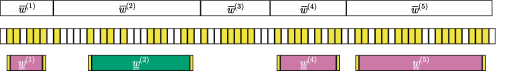
Figure 9: Illustration of the extraction of subwords $\underline{\underline{w}}^{(i)}$. The top row represents how the original string is parsed into words of the mZM parsing. In the middle row, the string is partitioned into strings of length $\ell_{*}\gg|{\mathfrak{c}}|$ and elements of the partitions are coloured (yellow) if the contain a copy of ${\mathfrak{c}}$. In the bottom row, the subwords are extracted, leaving so-called buffers between them. In particular, $2\in\mathcal{I}_{l}$ and $1,4,5\in\mathcal{I}_{g}$

type of $i$	type of $i\pm 1$	l.b. on $\underline{\underline{\ell}}_{i}$	l.b. on $|\xi_{\pm}^{(i)}|$	u.b. on $|\xi_{\pm}^{(i)}|$
$\mathcal{I}_{\mathrm{g}}$	$\mathcal{I}_{\mathrm{g}}$	$\ell_{-}-6\ell_{*}$	$2\ell_{*}$	$6\ell_{*}$
$\mathcal{I}_{\mathrm{g}}$	$\mathcal{I}_{\mathrm{l}}$	$\ell_{-}-6\ell_{*}$	$\ell_{*}+\eta\ell_{*}$	$3\ell_{*}+4\eta\ell_{*}$
$\mathcal{I}_{\mathrm{l}}$	$\mathcal{I}_{\mathrm{g}}$	$\eta\ell_{*}$	$\eta\ell_{*}+\ell_{*}$	$4\eta\ell_{*}+3\ell_{*}$
$\mathcal{I}_{\mathrm{l}}$	$\mathcal{I}_{\mathrm{l}}$	$\eta\ell_{*}$	$2\eta\ell_{*}$	$8\eta\ell_{*}$
$\mathcal{I}_{\mathrm{g}}$	$\mathcal{I}_{\mathrm{g}}^{\mathsf{c}}\cap\mathcal{I}_{\mathrm{l}}^{\mathsf{c}}$	$\ell_{-}-6\ell_{*}$	$\ell_{-}$	postponed to Step 4
$\mathcal{I}_{\mathrm{l}}$	$\mathcal{I}_{\mathrm{g}}^{\mathsf{c}}\cap\mathcal{I}_{\mathrm{l}}^{\mathsf{c}}$	$\eta\ell_{*}$	$\ell_{-}$	postponed to Step 4

Table 1: Description of the word $\underline{\underline{w}}^{(i)}$ for $i\in\mathcal{I}=\mathcal{I}_{\mathrm{g}}\sqcup\mathcal{I}_{\mathrm{l}}$ and its surrounding buffers for Step 3, depending on the type of $i\pm 1$.

Step 4.

We scan the $k$-th block $B_{k}$ from the Claim, from left to right, and note that for the $j$-th appearance of a “bad” word with $i\notin\mathcal{I}$ that starts within $B_{k}$ and satisfies $i-1\in\mathcal{I}$, there is some number $\tau_{j,k}$ of consecutive bad words that it is part of. Importantly, the last group of bad words starting within $B_{k}$ can go into $B_{k+1}$, but can cover at most $\eta$ words there. Let $J_{k}$ denote the number of distinct groups of bad words that start within $B_{k}$. Provided that $N$ is large enough, the Claim guarantees that

$$\sum_{j=1}^{J_{k}}\tau_{j,k}\leq 2\eta.$$

In (A.2), each group of consecutive bad words — spanning at most $\tau_{j,k}(9\eta\ell_{*})$ symbols — is joined with a leftovers from the neighbouring $i\in\mathcal{I}$ to form some $\xi_{\pm}^{(i)}$. These additional boundary strings are no longer than $4\eta\ell_{*}$. Therefore,

$$\mathcal{E}(N) \geq 2\sum_{k=1}^{D_{N}}\sum_{j=1}^{J_{k}}\ln\left(\mathrm{e}^{\gamma_{-}(17\eta\ell_{*}\tau_{j,k})^{\beta}}\right).$$

Now using that $\beta\geq 1$ and $\gamma_{-}<0$,

$$\sum_{k=1}^{D_{N}}\sum_{j=1}^{J_{k}}\ln\left(\mathrm{e}^{\gamma_{-}(17\eta\ell_{*}\tau_{j,k})^{\beta}}\right) =D_{N}\sum_{j=1}^{J_{k}}\gamma_{-}\left(17\eta\ell_{*}\tau_{j,k}\right)^{\beta}$$

$$\geq D_{N}\gamma_{-}\left(\sum_{j=1}^{J_{k}}17\eta\ell_{*}\tau_{j,k}\right)^{\beta}$$

$$\geq D_{N}\gamma_{-}34^{\beta}\eta^{2\beta}\ell_{*}^{\beta}$$

$$=-O\biggl{(}\frac{N}{\mathrm{e}^{\frac{K}{2}\ell_{*}}}(\ln N)^{2\beta-(\beta+1)\beta^{\prime}}\biggr{)}$$

$$=-o(N).$$

Hence, the proof will be complete once we have proved the Claim.

Proof of Claim..

Denote the $k$-th block in the construction by $B_{k}(y_{1}^{N})$. We will say that $B_{k}(y_{1}^{N})$ is ${\mathfrak{c}}$-sparse if more than $\eta$ of its members (intervals of length $\ell_{*}$) fail to contain ${\mathfrak{c}}$. Using again the Kontoyiannis argument for measures satisfying SLD, we get, for $N$ large enough,

$${\mathbb{Q}}\bigl{\{}y:W_{|{\mathfrak{c}}|}({\mathfrak{c}},y)>\ell_{*}-\tau_{\ell_{*}}-|{\mathfrak{c}}|\bigr{\}}\leq\exp\left(-k_{|{\mathfrak{c}}|}{\mathbb{Q}}[{\mathfrak{c}}]\left\lfloor\frac{\ell_{*}-|{\mathfrak{c}}|-\tau_{\ell_{*}}-1}{|{\mathfrak{c}}|+\tau_{|{\mathfrak{c}}|}}\right\rfloor\right)\leq\mathrm{e}^{-K\ell_{*}}$$

for some constant $K>0$. But then, by shift invariance and UD,

$${\mathbb{Q}}\left\{y:B_{k}(y_{1}^{N})\text{ is ${\mathfrak{c}}$-sparse}\right\} \leq\binom{\mathrm{e}^{\frac{K}{2}\ell_{*}}}{\eta}\left(\mathrm{e}^{k_{\ell_{*}}}{\mathbb{Q}}\bigl{\{}y:W_{|{\mathfrak{c}}|}({\mathfrak{c}},y)>\ell_{*}-\tau_{\ell_{*}}-|{\mathfrak{c}}|\bigr{\}}\right)^{\eta}$$

$$\leq\mathrm{e}^{\eta\frac{K}{2}\ell_{*}}\mathrm{e}^{\eta k_{\ell_{*}}}\mathrm{e}^{-\eta K\ell_{*}}$$

$$\leq N^{-3}$$

for $N$ large enough that ${k_{\ell_{*}}}\leq{\frac{K}{4}\ell_{*}}$. Hence, the Claim follows from a union bound over all $k$ and the Borel–Cantelli lemma in $N$. ∎

And that concludes the proof of the lemma. ∎

A.2 A Measure-theoretic lemma

The following lemma is an elementary estimate along the lines of the Markov inequality. However, because it is appealed to in the middle of a rather lengthy proof, we have opted to state and prove it separately.

Lemma A.1.

Let $\boldsymbol{\mu}$ be a finite Borel measure on ${\mathbb{R}}_{+}^{M}$. Suppose that there exists numbers $K,\varkappa>0$ and finite Borel measures $\mu_{1},\dotsc\mu_{M}$ on ${\mathbb{R}}_{+}$ such that the following properties hold:

1. as measures, $\boldsymbol{\mu}\leq K(\mu_{1}\otimes\dotsb\otimes\mu_{M})$;

2. for each $i=1,\dotsc,M$, the exponential moment $\mathfrak{m}_{i}:=\int\mathrm{e}^{\varkappa t}\mathop{\mathrm{\mathstrut d}}\nolimits\!\mu_{i}(t)$ is finite.

Then,

$$\boldsymbol{\mu}\left\{(t_{i})_{i=1}^{M}\in{\mathbb{R}}_{+}^{M}:\sum_{i=1}^{M}t_{i}\geq\tau\right\}\leq K\mathrm{e}^{-\varkappa\tau}\mathfrak{m}_{1}\dotsb\mathfrak{m}_{M}.$$

Proof.

Let $A_{\tau}:=\left\{(t_{i})_{i=1}^{M}\in{\mathbb{R}}_{+}^{M}:\sum_{i=1}^{M}t_{i}\geq\tau\right\}$. Then,

$$\boldsymbol{\mu}(A_{\tau}) \leq K\dotsint_{A_{\tau}}\mathop{\mathrm{\mathstrut d}}\nolimits\!\mu_{1}\dotsb\mathop{\mathrm{\mathstrut d}}\nolimits\!\mu_{M}$$

$$\leq K\dotsint_{A_{\tau}}\mathrm{e}^{\varkappa(\sum_{i=1}^{M}t_{i}-\tau)}\mathop{\mathrm{\mathstrut d}}\nolimits\!\mu_{1}(t_{1})\dotsb\mathop{\mathrm{\mathstrut d}}\nolimits\!\mu_{M}(t_{M})$$

$$\leq K\mathrm{e}^{-\varkappa\tau}\left(\int_{{\mathbb{R}}_{+}}\mathrm{e}^{\varkappa t_{1}}\mathop{\mathrm{\mathstrut d}}\nolimits\!\mu_{1}(t_{1})\right)\dotsb\left(\int_{{\mathbb{R}}_{+}}\mathrm{e}^{\varkappa t_{M}}\mathop{\mathrm{\mathstrut d}}\nolimits\!\mu_{M}(t_{M})\right),$$

as desired. ∎

Acknowledgements.

The authors would like to thank G. Cristadoro and V. Jakšić for stimulating discussions on the topic of this article. We are particularly grateful to N. Cuneo for sharing personal notes on generalizations of [BJPP18, §4.1], which allowed us to prove Lemma 3.5 and Theorem 3.8. The research of NB and RR was partially funded by the Fonds de recherche du Québec — Nature et technologies (FRQNT) and by the Natural Sciences and Engineering Research Council of Canada (NSERC). The research of RG was partially funded by the Rubin Gruber Science Undergraduate Research Award and Axel W Hundemer. The research of GP was done under the auspices of the Gruppo Nazionale di Fisica Matematica (GNFM) section of the Istituto Nazionale di Alta Matematica (INdAM). Part of this work was done during a stay of the four authors in Neuville-sur-Oise, funded by CY Initiative (grant Investissements d’avenir ANR-16-IDEX-0008).

References

- [AdACG22] M. Abadi, V. G. de Amorim, J.-R. Chazottes, and S. Gallo. Return-time -spectrum for equilibrium states with potentials of summable variation. Ergodic Theor. Dyn. Syst. (Online first), pages 1–27, 2022.
- [BBCDE08] C. Basile, D. Benedetto, E. Caglioti, and M. Degli Esposti. An example of mathematical authorship attribution. J. Math. Phys., 49(12), 2008.
- [BCJP21] T. Benoist, N. Cuneo, V. Jakšić, and C.-A. Pillet. On entropy production of repeated quantum measurements II. Examples. J. Stat. Phys., 182(3):1–71, 2021.
- [BCL02] D. Benedetto, E. Caglioti, and V. Loreto. Language trees and zipping. Phys. Rev. Lett., 88:048702, 2002.
- [BGPR23] N. Barnfield, R. Grondin, G. Pozzoli, and R. Raquépas. On the Ziv–Merhav theorem beyond Markovianity. Preprint, arXiv:2310.01367, 2023.
- [BJPP18] T. Benoist, V. Jakšić, Y. Pautrat, and C.-A. Pillet. On entropy production of repeated quantum measurements I. General theory. Commun. Math. Phys., 357(1):77–123, 2018.
- [CDEJR23] G. Cristadoro, M. Degli Esposti, V. Jakšić, and R. Raquépas. On a waiting-time result of Kontoyiannis: mixing or decoupling? Stoch. Proc. Appl., 166:104222, 2023.
- [CF05] D. P. Coutinho and M. A. Figueiredo. Information theoretic text classification using the Ziv–Merhav method. In J. S. Marques, N. Pérez de la Blanca, and P. Pina, editors, Pattern Recognition and Image Analysis, volume 3523 of Lecture Notes in Computer Science, pages 355–362. Springer, 2005.
- [CFH08] Y. Cao, D. Feng, and W. Huang. The thermodynamic formalism for sub-additive potentials. Discrete Contin. Dyn. Syst., 20(3):639, 2008.
- [CJPS19] N. Cuneo, V. Jakšić, C.-A. Pillet, and A. Shirikyan. Large deviations and fluctuation theorem for selectively decoupled measures on shift spaces. Rev. Math. Phys., 31(10):1950036, 2019.
- [CR23] N. Cuneo and R. Raquépas. Large deviations of return times and related entropy estimators on shift spaces. arXiv preprint, 2023. 2306.05277 [math.PR].
- [CU03] J.-R. Chazottes and E. Ugalde. Projection of Markov measures may be Gibbsian. J. Stat. Phys., 111(5/6):1245–1272, 2003.
- [Ell] R. S. Ellis. Entropy, large deviations, and statistical mechanics. Classics in mathematics. Springer-Verlag, 2006.
- [GS97] A. Galves and B. Schmitt. Inequalities for hitting times in mixing dynamical systems. Rand. Comput. Dyn., 5(4):337–348, 1997.
- [Kel] G. Keller. Equilibrium states in ergodic theory, volume 42 of London Mathematical Society Student Texts. Cambridge University Press, Cambridge, 1998.
- [Kie74] J. C. Kieffer. A simple proof of the Moy–Perez generalization of the Shannon–Mcmillan theorem. Pacific J. Math., 51(1):203–206, 1974.
- [Kon98] I. Kontoyiannis. Asymptotic recurrence and waiting times for stationary processes. J. Theor. Probab., 11(3):795–811, 1998.
- [LPS95] J. T. Lewis, C.-É. Pfister, and W. G. Sullivan. Entropy, concentration of probability and conditional limit theorems. Markov Proc. Relat. Fields, 1(3):319–386, 1995.
- [Moy61] S.-T. C. Moy. Generalizations of Shannon–McMillan theorem. Pacific J. Math., 11(2):705–714, 1961.
- [Ore85] S. Orey. On the Shannon–Perez–Moy theorem. Contemp. Math., 41:319–327, 1985.
- [PS20] C.-É. Pfister and W. G. Sullivan. Asymptotic decoupling and weak Gibbs measures for finite alphabet shift spaces. Nonlinearity, 33(9):4799–4817, 2020.
- [Raq23] R. Raquépas. A gapped generalization of Kingman’s subadditive ergodic theorem. J. Math. Phys., 64(6):06270, 2023.
- [Shi93] P. C. Shields. Waiting times: positive and negative results on the Wyner–Ziv problem. J. Theor. Probab., 6(3):499–519, 1993.
- [Sim] B. Simon. The Statistical Mechanics of Lattice Gases, volume 1. Princeton University Press, 1993.
- [Wal01] P. Walters. Convergence of the Ruelle operator for a function satisfying Bowen’s condition. Trans. Amer. Math. Soc., 353(1):327–347, 2001.
- [WZ89] A. D. Wyner and J. Ziv. Some asymptotic properties of the entropy of a stationary ergodic data source with applications to data compression. IEEE Int. Symp. Inf. Theory, 35(6):1250–1258, 1989.
- [Yoo10] J. Yoo. On factor maps that send Markov measures to Gibbs measures. J. Stat. Phys., 141(6):1055–1070, 2010.
- [ZM93] J. Ziv and N. Merhav. A measure of relative entropy between individual sequences with application to universal classification. IEEE Trans. Inf. Theory, 39(4):1270–1279, 1993.