Interacting Urns on Directed Networks with Node-Dependent Sampling and Reinforcement

Abstract

We consider interacting urns on a finite directed network, where both sampling and reinforcement processes depend on the nodes of the network. This extends previous research by incorporating node-dependent sampling (preferential or de-preferential) and reinforcement. We classify the reinforcement schemes and the networks on which the proportion of balls of either colour in each urn converges almost surely to a deterministic limit. We show that in case the reinforcement at all nodes is of Pólya-type, the limiting behaviour is very different from the node-independent sampling and a deterministic limit exists for certain networks classified by the distribution of preferential and de-preferential nodes across the network. We also investigate conditions for achieving synchronisation of the colour proportions across the urns. Further, we analyse fluctuations around the limit, under specific conditions on the reinforcement matrices and network structure.

1 Introduction

Interacting urn models have been studied extensively in recent times [2, 5, 10]. In an interacting urn system, each urn is reinforced based on the sampling of balls from itself or other urns in the system. Such processes exhibit interesting asymptotic behaviour and have applications across various fields. It is well-known that while in the classical two-colour Pólya urn model the fraction of balls of either colour converges almost surely to a random limit, a small change in the reinforcement leads to a deterministic limit (see [9]). In addition to the convergence for the interacting urns, the phenomenon of synchronisation (or consensus) is also of interest, particularly for studying applications of such models to opinion dynamics. Synchronisation refers to the convergence of the fraction of balls of each colour to the same limit across all urns. In [10] authors study a two-colour multi-urn process, where the evolution of each urn depends on itself (with probability $p$) as well as on all the other urns in the system (with probability $1-p$). Based on the value of the interaction parameter $p$, the authors also classify the sub-diffusive, diffusive and super-diffusive cases for the CLT-type limit theorems for the fluctuation of the fraction of balls of a colour around its limit. The interaction aspect of such models has been generalized to study urn processes (or more generally stochastic processes taking values in $[0,1]$) on finite networks in [1].

In this paper, we further extend the work in [1] by considering urns with balls of two colours located at the nodes of a finite directed network $\mbox{${\mathcal{G}}$}=(V,\mbox{${\mathcal{E}}$})$ such that each urn $i$ reinforces based a node-dependent reinforcement matrix $R_{i}$. At each time step, a ball is simultaneously and independently drawn from each urn, and the urn reinforces its out-neighbours as follows: if a white ball is drawn from the urn $i$, it reinforces all its out-neighbours with $[R_{i}]_{1,1}$ balls of white colour and $[R_{i}]_{1,2}$ balls of black colour. Similarly, if a black ball is drawn from the urn it reinforces all its out-neighbours with $[R_{i}]_{2,1}$ balls of white colour and $[R_{i}]_{2,2}$ balls of black colour. We assume balanced reinforcement matrices, that is the row sums of each $R_{i}$ are constant (say $m_{i}$). Nodes with zero in-degree are referred to as stubborn nodes as their associated urns remain unchanged throughout the process. We classify the urns or nodes as either Pólya or non-Pólya type based on the structure of their associated reinforcement matrices. By considering node-dependent reinforcement, this paper extends the work of [8], where the asymptotic properties of a similar interacting urn model with a fixed reinforcement scheme are studied.

In addition to node-based reinforcement, we also consider a mix of preferential and de-preferential sampling. That is, a white ball is drawn from an urn either with probability proportional to the fraction of white balls in the urn or with probability proportional to the fraction of black balls in the urn respectively. Such single urn processes have been studied before in [3, 7]. In this work, the authors consider an urn containing balls of $K$ different colours and a decreasing weight function to sample a ball from that urn. That is the colour with a higher proportion in the urn is less likely to be sampled. Then based on the reinforcement matrix, the authors show almost sure convergence of different colour proportions in the urn to a deterministic vector and also obtain central limit theorem type results.

In this paper, we classify the reinforcement type and graph structure on which the proportion of balls of either colour across all urns converges almost surely to a deterministic limit. This generalizes the result in [8]. Our results show that an almost sure deterministic limit exists if the graph and the reinforcement matrices are such that the influence of the stubborn nodes or that of a non-Pólya type urn reaches everywhere in the graph. In particular, on a strongly connected graph, a single node with non-Pólya type reinforcement is sufficient to achieve a deterministic limit for the fraction of balls of either colour across all urns. Further, when all nodes are of Pólya type, we show that the presence of de-preferential nodes may yield a deterministic limit and classify graphs (in terms of how preferential and de-preferential nodes are connected) on which this is possible. We also derive general conditions for synchronisation, where the fraction of balls of either colour converges to the same deterministic limit in each urn. Finally, CLT-type results for fluctuation of fraction of balls of a colour around its limit are stated and proved.

In the next section, we provide an overview of the interacting urn process. For a matrix $Q\in\mathbb{R}^{d\times d}$ and any subsets $S,F\subseteq[d]\coloneqq\{1,2,\dots,d\}$, we use the notation $Q_{SF}$ to represent the $|S|\times|F|$ matrix obtained by selecting elements from the index set $S\times F$. For simplicity, we write $Q_{S}$ instead of $Q_{SS}$, adopting an abuse of notation. Throughout the paper, $J$ denotes the matrix and $\mathbf{1}$ denotes the row vector, of appropriate dimensions respectively, with all elements equal to $1$.

2 Interacting Urn Process

Let $\mbox{${\mathcal{G}}$}=(V,\mbox{${\mathcal{E}}$})$ be a directed network, where $V=[N]$ represents the set of nodes and ${\mathcal{E}}$ represents the set of directed edges. For two nodes $i$ and $j$ in $V$, we use the notation $i\to j$ to indicate the presence of a directed edge from $i$ to $j$, and $i\rightsquigarrow j$ to denote the existence of a path $i=i_{0}\to i_{1}\to\dots\to i_{k-1}\to i_{k}=j$ from $i$ to $j$, where $i_{1},\dots,i_{k-1}\in V$. The in-degree and out-degree of a node $i$ are denoted by $d^{\mathrm{in}}_{i}\coloneqq|\{j\in V:j\to i\}|$ and $d^{\mathrm{out}}_{i}\coloneqq|\{j\in V:i\to j\}|$ respectively. The in-neighbourhood of node $i$ is denoted by $N_{i}\coloneqq\{j\in V:j\to i\}$. We consider networks ${\mathcal{G}}$ that do not contain any isolated nodes or nodes with a single self-loop i.e. there is no $i\in V$ such that $d^{\mathrm{in}}_{i}=d^{\mathrm{out}}_{i}=0$ or $N_{i}=\{i\}$. The former case is trivial and the latter case corresponds to a single urn reinforcing itself, which has been studied extensively (see [9]).

Following the approach in [8], the node set $V$ is partitioned into two disjoint sets: the set of stubborn nodes denoted by $S$ and the set of flexible nodes denoted by $F$. Specifically, we have $V=S\cup F$, where $S=\{i\in V:d^{\mathrm{in}}_{i}=0\}$ represents the stubborn nodes and $F=\{i\in V:d^{\mathrm{in}}_{i}>0\}$ represents the flexible nodes. Without loss of generality, we assume that the nodes labelled $1,\dots,|F|$ belong to the flexible set $F$. By adopting this labeling convention, the adjacency matrix $A$, with $(i,j)$ element denoted as $[A]_{i,j}=\mbox{${\mathbb{I}}$}_{\{i\to j\}}$, takes the following form:

$$\begin{pmatrix}A_{F}&\mathbf{0}\\ A_{SF}&\mathbf{0}\end{pmatrix}.$$

Suppose each node $i\in V$ has an urn that contains balls of two colours, white and black. Let $(W_{i}^{t},B_{i}^{t})$ be the configuration of the urn at node $i$, where $W_{i}^{t}$ and $B_{i}^{t}$ denote the number of white balls and black balls respectively and let $\mbox{${\mathbf{Z}}$}^{t}\coloneqq(Z_{1}^{t},\dots,Z_{N}^{t})$, where $Z_{i}^{t}=\frac{W_{i}^{t}}{W_{i}^{t}+B_{i}^{t}}$, at time $t\geq 0$. Let the total number of balls in the urn at node $i$ at time $t$ is $T_{i}^{t}$, i.e. $T_{i}^{t}=W_{i}^{t}+B_{i}^{t}$. Given the configuration ${(W_{i}^{t},B_{i}^{t})}_{i\in V}$ at time $t$, we update the configuration of each urn at time $t+1$ using the following two steps:

1. Sampling: At each time step, a ball is selected from each urn. Let $\chi_{i}^{t}$ denote the indicator of the event that a white ball is drawn from the urn at node $i$ at time $t$. We consider preferential and de-preferential sampling. Let $\mbox{${\mathcal{P}}$},\mbox{${\mathcal{D}}$}$ denote the set of nodes with preferential and de-preferential sampling respectively. Then conditioned on $\mbox{${\mathcal{F}}$}_{t}=\sigma\left(\mbox{${\mathbf{Z}}$}^{0},\mbox{${\mathbf{Z}}$}^{1},\ldots,\mbox{${\mathbf{Z}}$}^{t}\right)$, $\{\chi_{i}^{t+1}\}_{i\in V}$ are independent random variables such that

   $$\text{ for }i\in\mbox{${\mathcal{P}}$}\qquad\chi_{i}^{t+1} =\begin{cases}1&\text{ with probability }Z^{t}_{i}\\ 0&\text{ with probability }1-Z^{t}_{i}\end{cases}$$

   $$\text{ and for }i\in\mbox{${\mathcal{D}}$}\qquad\chi_{i}^{t+1} =\begin{cases}1&\text{ with probability }1-Z^{t}_{i}\\ 0&\text{ with probability }Z^{t}_{i}\end{cases}.$$ (1)

   After we record the colours of the selected balls in vector $\chi^{t+1}$, we put the balls back into their respective urns.

2. Reinforcement: Let $m_{i}\in\mbox{${\mathbb{Z}}$}_{+}$ and $\alpha_{i},\beta_{i}\in\{0,1,\dots,m_{i}\}$ be fixed non-negative integers. For each node $i\in V$, if a white ball is selected (in the sampling step) from the urn at node $i$, $\alpha_{i}$ white balls and $m_{i}-\alpha_{i}$ black balls are added to each urn $j$ such that $i\to j$. On the other hand, if a black ball is selected from the urn at node $i$, $m_{i}-\beta_{i}$ white balls and $\beta_{i}$ black balls are added to each urn $j$ such that $i\to j$. In other words, the urn at node $i$ reinforces its out-neighbours according to the reinforcement matrix $R_{i}=\begin{pmatrix}\alpha_{i}&m_{i}-\alpha_{i}\\ m_{i}-\beta_{i}&\beta_{i}\end{pmatrix}$. We classify the type of reinforcement by node $i$ as follows.

   1. Pólya type: if $\alpha_{i}=\beta_{i}=m_{i}$, which corresponds to $R_{i}=m_{i}I$.

   2. non-Pólya type: if $0<\alpha_{i}+\beta_{i}<2m_{i}$.

Note that, although we consider $\alpha_{i},\beta_{i}\in\mbox{${\mathbb{Z}}$}_{\geq 0}$, it is worth mentioning that the arguments in this paper apply to all balanced matrices with entries in $\mbox{${\mathbb{R}}$}_{\geq 0}$. The interacting urn dynamics defined above can be expressed as the following recursive relation:

$$W_{i}^{t+1} =W_{i}^{t}+\sum_{j\in N_{i}}\left[\alpha_{j}\chi_{j}^{t+1}+(m_{j}-\beta_{j})(1-\chi_{j}^{t+1})\right],$$

$$B_{i}^{t+1} =B_{i}^{t}+\sum_{j\in N_{i}}\left[m_{j}-\alpha_{j}\chi_{j}^{t+1}+\beta_{j}(1-\chi_{j}^{t+1})\right],\quad\quad\forall i\in V.$$ (2)

Remark 1.

We have omitted the case when $\alpha_{i}+\beta_{i}=0$ (and $\alpha_{i}+\beta_{i}=2m_{i}$ in general other than the sub-case covered under a special case in Theorem 3.1). The only instance of $\alpha_{i}+\beta_{i}=0$ is when both values are zero. In this case, the reinforcement matrix is given by $\begin{pmatrix}0&m_{i}\\ m_{i}&0\end{pmatrix}$. It is worth noting that preferential sampling with this reinforcement matrix is essentially the same as de-preferential sampling with Pólya-type reinforcement. However, (as we shall see later) in certain cases, this reinforcement scheme doesn’t lead to a deterministic limit. We do not address the limiting behaviour in these cases as in this paper we aim to analyse the cases where $\mbox{${\mathbf{Z}}$}^{t}$ converges to a deterministic limit.

Observe that the urns at stubborn nodes are not reinforced and therefore their configurations remain unchanged throughout the process. Before we proceed to state and prove our main results, we fix some notation. We define $a_{i}=\alpha_{i}/m_{i}$ and $b_{i}=\beta_{i}/m_{i}$ and denote $\mbox{a}=(a_{1},\dots,a_{N})$ and $\mbox{b}=(b_{1},\ldots,b_{N})$. The total reinforcement at node $i$ is represented by $\mbox{$\overline{m}$}_{i}=\sum_{j\in N_{i}}m_{j}$. We define the diagonal matrices $B=\mathop{\mathrm{Diag}}(a_{1}+b_{1}-1,\dots,a_{N}+b_{N}-1)$, $\mbox{${\mathbf{T}}$}^{t}=\mathop{\mathrm{Diag}}(T_{1}^{t},\dots,T_{N}^{t})$, $M=\mathop{\mathrm{Diag}}(m_{1},\dots,m_{N})$, and $\mbox{$\overline{M}$}=\mathop{\mathrm{Diag}}(\mbox{$\overline{m}$}_{1},\dots,\mbox{$\overline{m}$}_{|F|},0,\dots,0)$ as $\mbox{$\overline{m}$}_{i}=0$ for every $i\in S$. Additionally, we define the scaled adjacency matrix $\mbox{$\widetilde{A}$}=MA\mbox{$\overline{M}$}^{-1}$, which is of the form $\mbox{$\widetilde{A}$}=\begin{pmatrix}\mbox{$\widetilde{A}$}_{F\cap\mbox{${\scriptstyle\mathcal{P}}$},F\cap\mbox{${\scriptstyle\mathcal{P}}$}}&\mbox{$\widetilde{A}$}_{F\cap\mbox{${\scriptstyle\mathcal{P}}$},F\cap\mbox{${\scriptstyle\mathcal{D}}$}}&\mathbf{0}&\mathbf{0}\\ \mbox{$\widetilde{A}$}_{F\cap\mbox{${\scriptstyle\mathcal{D}}$},F\cap\mbox{${\scriptstyle\mathcal{P}}$}}&\mbox{$\widetilde{A}$}_{F\cap\mbox{${\scriptstyle\mathcal{D}}$},F\cap\mbox{${\scriptstyle\mathcal{D}}$}}&\mathbf{0}&\mathbf{0}\\ \mbox{$\widetilde{A}$}_{S\cap\mbox{${\scriptstyle\mathcal{P}}$},F\cap\mbox{${\scriptstyle\mathcal{P}}$}}&\mbox{$\widetilde{A}$}_{S\cap\mbox{${\scriptstyle\mathcal{P}}$},F\cap\mbox{${\scriptstyle\mathcal{D}}$}}&\mathbf{0}&\mathbf{0}\\ \mbox{$\widetilde{A}$}_{S\cap\mbox{${\scriptstyle\mathcal{P}}$},F\cap\mbox{${\scriptstyle\mathcal{P}}$}}&\mbox{$\widetilde{A}$}_{S\cap\mbox{${\scriptstyle\mathcal{D}}$},F\cap\mbox{${\scriptstyle\mathcal{D}}$}}&\mathbf{0}&\mathbf{0}\\ \end{pmatrix}.$ Now we define a diagonal matrix

$$\mbox{${\mathcal{I}}$}=\begin{pmatrix}I_{F\cap\mbox{${\scriptstyle\mathcal{P}}$}}&\mathbf{0}&\mathbf{0}&\mathbf{0}\\ \mathbf{0}&-I_{F\cap\mbox{${\scriptstyle\mathcal{D}}$}}&\mathbf{0}&\mathbf{0}\\ \mathbf{0}&\mathbf{0}&I_{S\cap\mbox{${\scriptstyle\mathcal{P}}$}}&\mathbf{0}\\ \mathbf{0}&\mathbf{0}&\mathbf{0}&-I_{S\cap\mbox{${\scriptstyle\mathcal{D}}$}}\end{pmatrix},$$

where $I$ is the $N\times N$ identity matrix.

In the next section, we describe an exploration process on the graph ${\mathcal{G}}$. The process begins at an arbitrary node $v\in V$ and explores its neighbourhood in the next step. As the exploration continues we assign each node to a subset of $V$, based on its sampling-type and the sampling-type of nodes in its in-neighbourhood. When each node has a unique assignment, it results in a partition of $V$ into $4$ disjoint subsets. Thus, it classifies all finite directed graphs into two categories: graphs that admit partition via the exploration process and graphs that don’t admit a partition.

2.1 Exploration Process on the Graph

For a graph $\mbox{${\mathcal{G}}$}=(V,\mbox{${\mathcal{E}}$})$, where $V=\mbox{${\mathcal{P}}$}\cup\mbox{${\mathcal{D}}$}$, we start the exploration process from any node $v$ and depending on its sampling-type we assign it to $P_{1}$ or $D_{1}$, where $P_{1}\subseteq\mbox{${\mathcal{P}}$}$ and $D_{1}\subseteq\mbox{${\mathcal{D}}$}$. In the subsequent steps, the process explores nodes in the graph and categorizes them into four sets, $P_{1},P_{2},D_{1},D_{2}$, based on the sampling type of their in-neighbours (preferential or de-preferential).

Algorithm 1 Graph Exploration Process

Input: A directed graph $\mbox{${\mathcal{G}}$}(V,E)$ and the sets of preferential nodes ${\mathcal{P}}$ and de-preferential nodes ${\mathcal{D}}$.
Output: Whether ${\mathcal{G}}$ admits a partition or not.

1:  Select a node $j\in V$

2:  if $j\in\mbox{${\mathcal{P}}$}$ then

3:     Initialize $P_{1}\leftarrow\{j\}$, $P_{2}=D_{1}=D_{2}=\emptyset$.

4:  else

5:     Initialize $D_{1}\leftarrow\{j\}$, $P_{1}=P_{2}=D_{2}=\emptyset$.

6:  end if

7:  while $(P_{1}\cup P_{2}\cup D_{1}\cup D_{2})\subsetneq V$ do

8:     $P_{1}\leftarrow P_{1}\cup\left(\cup_{j\in P_{1}}N_{j}\cap\mbox{${\mathcal{P}}$}\right)$ and $D_{1}\leftarrow D_{1}\cup\left(\cup_{j\in P_{1}}N_{j}\cap\mbox{${\mathcal{D}}$}\right)$

9:     $P_{2}\leftarrow P_{2}\cup\left(\cup_{j\in D_{1}}N_{j}\cap\mbox{${\mathcal{P}}$}\right)$ and $D_{2}\leftarrow D_{2}\cup\left(\cup_{j\in D_{1}}N_{j}\cap\mbox{${\mathcal{D}}$}\right)$

10:     $P_{1}\leftarrow P_{1}\cup\left(\cup_{j\in D_{2}}N_{j}\cap\mbox{${\mathcal{P}}$}\right)$ and $D_{1}\leftarrow D_{1}\cup\left(\cup_{j\in D_{2}}N_{j}\cap\mbox{${\mathcal{D}}$}\right)$

11:     $P_{2}\leftarrow P_{2}\cup\left(\cup_{j\in P_{2}}N_{j}\cap\mbox{${\mathcal{P}}$}\right)$ and $D_{2}\leftarrow D_{2}\cup\left(\cup_{j\in P_{2}}N_{j}\cap\mbox{${\mathcal{D}}$}\right)$

12:     if $P_{1},P_{2},D_{1},D_{2}$ are not mutually disjoint then

13:        BREAK and return “${\mathcal{G}}$ does not admit a Graph partition.”

14:     end if

15:  end while

16:  Repeat Steps 8 to Step 11 once.

17:  if  any node is re-assigned from $P_{1}$ to $P_{2}$ (or vice versa) or from $D_{1}$ to $D_{2}$ (or vice versa) then

18:     return “${\mathcal{G}}$ does not admit a Graph partition”

19:  else

20:     return “${\mathcal{G}}$ admits a Graph partition $G(P_{1},P_{2},D_{1},D_{2})$, such that $\mbox{${\mathcal{P}}$}=P_{1}\cup P_{2}$ and $\mbox{${\mathcal{D}}$}=D_{1}\cup D_{2}$”

21:  end if

If a graph partition exists, it is determined; otherwise, the algorithm returns that no such partition is possible. Note that, this algorithm for graph partitioning remains invariant with respect to the initial selection of the node $j$, upto a permutation of sets $(P_{1},P_{2},D_{1},D_{2})$. The exploration process in Algorithm 1 is illustrated in Figure 1.

Figure 1: The figure describes the exploration process for the graph partition $\mbox{${\mathcal{G}}$}(P_{1},P_{2},D_{1},D_{2})$, as described in Step 8 to Step 11 of Algorithm 1. The arrows represent the directed edges, where for instance an arrow from $D_{1}$ to $P_{1}$ means that there exists $u\in D_{1}$ and $v\in P_{1}$ such that $u\to v$ in ${\mathcal{G}}$.

We now provide a few examples to illustrate different cases.

Example 2.1 (Graph that does not admit a partition).

Suppose $F=\mbox{${\mathcal{P}}$}\cup\mbox{${\mathcal{D}}$}$ is such that it is strongly connected and there is only one node in the set ${\mathcal{D}}$, represented as $\mbox{${\mathcal{D}}$}=\{\mathfrak{d}\}$. Let $j\in\mbox{${\mathcal{P}}$}$ be the node selected at Step 1 of Algorithm 1, that is, $j\in P_{1}$. Since $F$ is strongly connected, there exists a path $\mathfrak{d}\rightsquigarrow j$ such that all nodes on the path are preferential, implying $\mathfrak{d}$ must be in set $D_{1}$ (see Step 8 of Algorithm 1). Similarly, $j\rightsquigarrow\mathfrak{d}$ via a path of preferential nodes, implying that $j\in P_{2}$ (see Step 9 of Algorithm 1 or see Figure 1). A similar conclusion holds if the node selected at step 1 is $\mathfrak{d}$. Thus, such a graph does not admit a valid partition. To illustrate this, we consider a special case of a strongly connected graph with one de-preferential node in Figure 2.

Figure 2: A graph with 8 nodes with $\mbox{${\mathcal{P}}$}=\{1,2,3,4,5,6,7\}$ and $\mbox{${\mathcal{D}}$}=\{8\}$. Suppose in the Step 3 of Algorithm 1 we initialize with $P_{1}=\{1\},P_{2}=D_{1}=D_{2}=\emptyset$. Then following the algorithm Steps 8 to Step 11, we get $D_{1}=\{8\}$ and $P_{2}=\{2,3,4,5,6,7\},D_{2}=\emptyset$. However, in Step 16, node 1 gets reassigned to $P_{2}$. Therefore, the graph does not admit a graph partition under Algorithm 1.

Example 2.2 (Graph that admits a partition).

Consider an even cycle of size $2k$ with alternate preferential and de-preferential nodes. In this case, starting with $1\in P_{1}$, the algorithm terminates with a valid assignment of nodes to the four sets, namely, $P_{1}=\{1,3,\dots,k-1\},P_{2}=\{2,4,\dots,k\},D_{1}=\{k+1,k+3,\dots,2k-1\}$ and $D_{2}=\{k+2,k+4,\dots,2k\}$. Figure 3 illustrates the case for $k=4$.

Figure 3: A graph with 8 nodes with $\mbox{${\mathcal{P}}$}=\{1,2,3,4\}$ and $\mbox{${\mathcal{D}}$}=\{5,6,7,8\}$ that results in a valid partition via the given exploration process. In particular, we get $P_{1}=\{1,3\}$, and $P_{2}=\{2,4\}$, $D_{1}=\{6,8\}$, $D_{2}=\{5,7\}$.

In fact, it is easy to see that a cycle graph with an odd number of de-preferential nodes does not admit a valid partition whereas, a cycle graph with an even number of de-preferential nodes has a valid partition.

In the next section (Section 3), we state and prove the convergence and synchronisation results for $\mbox{${\mathbf{Z}}$}^{t}$. In Section 4, we prove CLT type limit theorems for $\mbox{${\mathbf{Z}}$}^{t}$. In the last section (Section 5), we discuss some examples with simulations.

3 Convergence Results

Theorem 3.1 (Convergence of $\mbox{${\mathbf{Z}}$}^{t}$).

Suppose $F$ is strongly connected and one of the following conditions holds:

1. There exists a node $f\in F$ that is of non-Pólya type.

2. $S\neq\emptyset$.

3. All nodes in $F$ are of Pólya type and $F$ does not admit a valid graph partition under Algorithm 1.

Then $\mbox{${\mathbf{Z}}$}^{t}\xrightarrow{a.s.}\mbox{${\mathbf{Z}}$}^{\star}\ \text{ as }t\to\infty$ where $\mbox{${\mathbf{Z}}$}^{\star}$ is of the form $(\mbox{${\mathbf{Z}}$}^{\star}_{F},\mbox{${\mathbf{Z}}$}^{0}_{S})$ such that

$$\mbox{${\mathbf{Z}}$}_{F}^{\star}=\big{[}\mbox{${\mathbf{Z}}$}_{S}^{0}(\mbox{${\mathcal{I}}$}B\mbox{$\widetilde{A}$})_{SF}+({\bf e}B\mbox{$\widetilde{A}$})_{F}+((\mathbf{1}-\mbox{b})\mbox{$\widetilde{A}$})_{F}\big{]}\left(I-(\mbox{${\mathcal{I}}$}B\mbox{$\widetilde{A}$})_{F}\right)^{-1},$$ (3)

with ${\bf e}=\left(\mathbf{0}_{F\cap\mbox{${\scriptstyle\mathcal{P}}$}},\mathbf{1}_{F\cap\mbox{${\scriptstyle\mathcal{D}}$}},\mathbf{0}_{S\cap\mbox{${\scriptstyle\mathcal{P}}$}},\mathbf{1}_{S\cap\mbox{${\scriptstyle\mathcal{D}}$}}\right)$.

Remark 2.

The general case of the Pólya type urn process where the underlying graph does not satisfy condition (iii) of Theorem 3.1 is left as future work. We discuss the two extreme cases when all noses in $F$ are Pólya type:

• when $\mbox{${\mathcal{P}}$}=\emptyset$, then $F$ admits a partition under the exploration process if and only if $F$ is a bipartite digraph with node sets $D_{1}$ and $D_{2}$. Note that this case is equivalent to the case discussed in Remark 1 where the reinforcement is such that $\alpha_{i}=\beta_{i}=0$ and $m_{i}=m\ \forall i\in V$. A similar case on the undirected bipartite graph, albeit for urns with multiple drawings, has been studied in [6].

• when $\mbox{${\mathcal{D}}$}=\emptyset$, in [8] it was shown that on a regular directed graph, with $m_{i}=m$ for all $i$ and some additional conditions, while the asymptotic limit is random, the urns synchronise in the sense that fraction of balls of either colour converges to the same random limit almost surely.

The above theorem can be generalized to get the following convergence result on a weakly connected graph.

Corollary 3.2.

Suppose $F$ is weakly connected with strongly connected components $F_{1},F_{2},\dots,F_{k}$, such that the adjacency matrix is of the form

$$A_{F}=\begin{pmatrix}A_{F_{1}}&A_{F_{1}F_{2}}&\dots&A_{F_{1}F_{k}}\\ \mathbf{0}&A_{F_{2}}&\dots&A_{F_{2}F_{k}}\\ \vdots&\vdots&\ddots&\vdots\\ \mathbf{0}&\mathbf{0}&\dots&A_{F_{k}}\end{pmatrix},$$

where $A_{F_{i}F_{j}}$ is a $|F_{i}|\times|F_{j}|$ matrix. Suppose condition (i) or (iii) of Theorem 3.1 hold for $F_{1}$, or condition (ii) holds such that there exists a node $s\in S$ and $f\in F_{1}$ such that $s\to f$. Then as $t\to\infty$, $\mbox{${\mathbf{Z}}$}^{t}\xrightarrow{a.s.}\mbox{${\mathbf{Z}}$}^{\star}$, where $\mbox{${\mathbf{Z}}$}^{\star}$ is as given in equation (3).

Next, we explore the conditions for synchronisation, that is when the limiting fraction of balls of each colour is the same for every urn. For this purpose, we outline conditions that are sufficient to ensure synchronisation within the framework of Theorem 3.1.

• There exist $\mu_{F}\geq 0$ such that $\mathbf{1}(\mbox{${\mathcal{I}}$}B\mbox{$\widetilde{A}$})_{F}=\mu_{F}\mathbf{1}$, i.e. for every $j\in F$, $\sum_{i\in F\cap N_{j}}\mbox{${\mathcal{I}}$}_{i,i}\frac{(\alpha_{i}+\beta_{i}-m_{i})}{\mbox{$\overline{m}$}_{j}}=\mu_{F}$.

• There exist $\mu_{S}\geq 0$ such that $\mbox{${\mathbf{Z}}$}_{S}^{0}(\mbox{${\mathcal{I}}$}B\mbox{$\widetilde{A}$})_{SF}=\mu_{S}\mathbf{1}$, i.e. for every $j\in F$, $\sum_{i\in S\cap N_{j}}Z_{i}^{0}\frac{(\alpha_{i}+\beta_{i}-m_{i})}{\mbox{$\overline{m}$}_{j}}=\mu_{S}$.

• There exist $\delta\geq 0$ such that $\big{(}{\bf e}B\mbox{$\widetilde{A}$}\big{)}_{F}+\big{(}(\mathbf{1}-\mbox{b})\mbox{$\widetilde{A}$}\big{)}_{F}=\delta\mathbf{1}$, i.e. for every $j\in F$, $\sum_{i\in\mbox{${\scriptstyle\mathcal{D}}$}\cap N_{j}}\frac{(\alpha_{i}+\beta_{i}-m_{i})}{\mbox{$\overline{m}$}_{j}}+\sum_{i\in N_{j}}\frac{m_{i}-\beta_{i}}{\mbox{$\overline{m}$}_{j}}=\delta$.

Corollary 3.3 (Synchronisation).

Suppose the conditions of Theorem 3.1 hold. Then, under the synchronisation conditions (SC1), (SC2) and (SC3),

$$Z_{i}^{t}\xrightarrow{a.s.}z^{\star}=\frac{\delta+\mu_{S}}{1-\mu_{F}},\quad\text{ as }t\to\infty\text{ for every }i\in F.$$

Remark 3.

Note that these conditions are only sufficient and not necessary. For instance, on a cycle graph with all Pólya type nodes such that only one node is de-preferential, while condition (iii) of Theorem 3.1 holds (as seen in Example 2.1), (SC1) does not hold. However, it is easy to check that the fraction of balls of either colour synchronises to a deterministic limit of $1/2$.

Corollary 3.4 (Synchronisation in absence of de-preferential nodes).

Suppose there are no de-preferential nodes and either condition (i) or (ii) of Theorem 3.1 hold. Further, suppose the following conditions hold.

• There exist $\alpha^{F},\beta^{F},\beta^{S},m^{F},m^{S}\in\mbox{${\mathbb{Z}}$}_{\geq 0}$ with $\alpha^{F}+\beta^{F}<2m^{F}+m^{S}$, such that for every $i\in F$, $\sum\limits_{j\in N_{i}\cap S}m_{j}=m^{S},\sum\limits_{j\in N_{i}\cap S}\beta_{j}=\beta^{S}$ and

  $$\sum\limits_{j\in N_{i}\cap F}R_{j}=\begin{pmatrix}\alpha^{F}&m^{F}-\alpha^{F}\\ m^{F}-\beta^{F}&\beta^{F}\end{pmatrix}.$$

• If $S\neq\emptyset$, there exist $\alpha^{0,S},\beta^{0,S},m^{0,S}\in\mbox{${\mathbb{Z}}$}_{\geq 0}$ such that for every $i\in F$

  $$\sum\limits_{j\in N_{i}\cap S}Z_{j}^{0}R_{j}=\begin{pmatrix}\alpha^{0,S}&m^{0,S}-\alpha^{0,S}\\ m^{0,S}-\beta^{0,S}&\beta^{0,S}\end{pmatrix}.$$

Then

$$Z_{i}^{t}\xrightarrow{a.s.}z^{\star}=\frac{m^{F}+m^{S}-\beta^{F}-\beta^{S}-(m^{0,S}-\alpha^{0,S}-\beta^{0,S})}{2m^{F}+m^{S}-\alpha^{F}-\beta^{F}},\quad\text{ as }t\to\infty\text{ for every }i\in F.$$

In particular, if $S=\emptyset$ and synchronisation condition (PSC1) holds, then $Z_{i}^{t}\xrightarrow{a.s.}\frac{m^{F}-\beta^{F}}{2m^{F}-\alpha^{F}-\beta^{F}}$, as $t\to\infty$, for every $i\in V$.

3.1 Proofs of Convergence Results

The main tool in analyzing the asymptotic properties of the fraction of white balls across urns is to write an appropriate stochastic approximation scheme (see [4, 11]) for the vector $\mbox{${\mathbf{Z}}$}^{t}_{F}$. Using (1) and (2), we derive the recursion for the proportion of white balls in the urn at node $i\in F$ as follows:

$$Z_{i}^{t+1} =\frac{1}{T_{i}^{t+1}}W_{i}^{t+1}$$

$$=\frac{T_{i}^{t}}{T_{i}^{t+1}}Z_{i}^{t}+\frac{1}{T_{i}^{t+1}}\sum_{j\in N_{i}}\left[\alpha_{j}\chi_{j}^{t+1}+(m_{j}-\beta_{j})(1-\chi_{j}^{t+1})\right]$$ (4)

$$=Z_{i}^{t}-\frac{\mbox{$\overline{m}$}_{i}}{T_{i}^{t+1}}Z_{i}^{t}+\frac{1}{T_{i}^{t+1}}\sum_{j\in N_{i}\cap F}m_{j}(\alpha_{j}+b_{j}-1)\chi_{j}^{t+1}+\frac{1}{T_{i}^{t+1}}\sum_{j\in N_{i}\cap S}m_{j}(a_{j}+b_{j}-1)\chi_{j}^{t+1}$$

$$+\frac{1}{T_{i}^{t+1}}\sum_{j\in N_{i}}m_{j}(1-b_{j})$$ (5)

$$=Z_{i}^{t}-\frac{\mbox{$\overline{m}$}_{i}}{T_{i}^{t+1}}Z_{i}^{t}+\frac{1}{T_{i}^{t+1}}\sum_{j\in N_{i}\cap F\cap\mbox{${\scriptstyle\mathcal{P}}$}}m_{j}(a_{j}+b_{j}-1)Z_{j}^{t}+\frac{1}{T_{i}^{t+1}}\sum_{j\in N_{i}\cap F\cap\mbox{${\scriptstyle\mathcal{D}}$}}m_{j}(a_{j}+b_{j}-1)(1-Z_{j}^{t})$$

$$\quad+\frac{1}{T_{i}^{t+1}}\sum_{j\in N_{i}\cap S\cap\mbox{${\scriptstyle\mathcal{P}}$}}m_{j}(a_{j}+b_{j}-1)Z_{j}^{0}+\frac{1}{T_{i}^{t+1}}\sum_{j\in N_{i}\cap S\cap\mbox{${\scriptstyle\mathcal{P}}$}}m_{j}(a_{j}+b_{j}-1)(1-Z_{j}^{0})$$

$$\quad+\frac{1}{T_{i}^{t+1}}\sum_{j\in N_{i}}m_{j}(1-b_{j})+\frac{1}{T_{i}^{t+1}}\sum_{j\in N_{i}}m_{j}(a_{j}+b_{j}-1)\Delta\chi_{j}^{t+1}.$$ (6)

where $\Delta\chi_{j}^{t+1}=\chi_{j}^{t+1}-\mbox{${\mathbb{E}}$}[\chi_{j}^{t+1}|\mbox{${\mathcal{F}}$}_{t}]$ is a martingale difference sequence. Now, we write the above recursion in vector form as follows:

$$\mbox{${\mathbf{Z}}$}^{t+1}_{F} =\mbox{${\mathbf{Z}}$}^{t}_{F}+\left[h(\mbox{${\mathbf{Z}}$}^{t}_{F})+(\Delta\chi^{t+1}B\mbox{$\widetilde{A}$})_{F}\right]\mbox{$\overline{M}$}_{F}\left(\mbox{${\mathbf{T}}$}^{t+1}_{F}\right)^{-1}$$ (7)

$$=\mbox{${\mathbf{Z}}$}^{t}_{F}+\frac{1}{t+1}\left[h(\mbox{${\mathbf{Z}}$}^{t}_{F})+(\Delta\chi^{t+1}B\mbox{$\widetilde{A}$})_{F}\right]\mbox{$\overline{M}$}_{F}+\epsilon_{t},$$ (8)

where $\epsilon_{t}=\mbox{${\mathbf{Z}}$}^{t}_{F}+\left[h(\mbox{${\mathbf{Z}}$}^{t}_{F})+(\Delta\chi^{t+1}B\mbox{$\widetilde{A}$})_{F}\right]\mbox{$\overline{M}$}_{F}\left(\left(\mbox{${\mathbf{T}}$}^{t+1}_{F}\right)^{-1}-\frac{1}{t+1}\right)$ and the function $h:[0,1]^{|F|}\to[0,1]^{|F|}$ is such that

$$h(\mbox{${\mathbf{Z}}$}_{F}) =-\mbox{${\mathbf{Z}}$}_{F}+\left(\mbox{${\mathbf{Z}}$}_{F\cap\mbox{${\scriptstyle\mathcal{P}}$}},\mathbf{1}-\mbox{${\mathbf{Z}}$}_{F\cap\mbox{${\scriptstyle\mathcal{D}}$}}\right)(B\mbox{$\widetilde{A}$})_{F}+\left(\mbox{${\mathbf{Z}}$}_{S\cap\mbox{${\scriptstyle\mathcal{P}}$}}^{0},\mathbf{1}-\mbox{${\mathbf{Z}}$}_{S\cap\mbox{${\scriptstyle\mathcal{D}}$}}^{0}\right)(B\mbox{$\widetilde{A}$})_{SF}+((\mathbf{1}-\mbox{b})\mbox{$\widetilde{A}$})_{F}$$

$$=-\mbox{${\mathbf{Z}}$}_{F}+\mbox{${\mathbf{Z}}$}_{F}\begin{pmatrix}I_{F\cap\mbox{${\scriptstyle\mathcal{P}}$}}&\mathbf{0}\\ \mathbf{0}&-I_{F\cap\mbox{${\scriptstyle\mathcal{D}}$}}\end{pmatrix}(B\mbox{$\widetilde{A}$})_{F}+\mbox{${\mathbf{Z}}$}_{S}^{0}\begin{pmatrix}I_{S\cap\mbox{${\scriptstyle\mathcal{P}}$}}&\mathbf{0}\\ \mathbf{0}&-I_{S\cap\mbox{${\scriptstyle\mathcal{D}}$}}\end{pmatrix}(B\mbox{$\widetilde{A}$})_{SF}$$

$$\quad+\left(\mathbf{0}_{F\cap\mbox{${\scriptstyle\mathcal{P}}$}},\mathbf{1}_{F\cap\mbox{${\scriptstyle\mathcal{D}}$}}\right)(B\mbox{$\widetilde{A}$})_{F}+\left(\mathbf{0}_{S\cap\mbox{${\scriptstyle\mathcal{P}}$}},\mathbf{1}_{S\cap\mbox{${\scriptstyle\mathcal{D}}$}}\right)(B\mbox{$\widetilde{A}$})_{SF}+((\mathbf{1}-\mbox{b})\mbox{$\widetilde{A}$})_{F}$$

$$=-\mbox{${\mathbf{Z}}$}_{F}+\mbox{${\mathbf{Z}}$}_{F}\begin{pmatrix}I_{F\cap\mbox{${\scriptstyle\mathcal{P}}$}}&\mathbf{0}\\ \mathbf{0}&-I_{F\cap\mbox{${\scriptstyle\mathcal{D}}$}}\end{pmatrix}(B\mbox{$\widetilde{A}$})_{F}+\mbox{${\mathbf{Z}}$}_{S}^{0}\begin{pmatrix}I_{S\cap\mbox{${\scriptstyle\mathcal{P}}$}}&\mathbf{0}\\ \mathbf{0}&-I_{S\cap\mbox{${\scriptstyle\mathcal{D}}$}}\end{pmatrix}(B\mbox{$\widetilde{A}$})_{SF}+(\bf{e}B\mbox{$\widetilde{A}$})_{F}+((\mathbf{1}-\mbox{b})\mbox{$\widetilde{A}$})_{F}$$

$$=-\mbox{${\mathbf{Z}}$}_{F}\left[I-(\mbox{${\mathcal{I}}$}B\mbox{$\widetilde{A}$})_{F}\right]+\mbox{${\mathbf{Z}}$}_{S}^{0}(\mbox{${\mathcal{I}}$}B\mbox{$\widetilde{A}$})_{SF}+({\bf e}B\mbox{$\widetilde{A}$})_{F}+((\mathbf{1}-\mbox{b})\mbox{$\widetilde{A}$})_{F},$$ (9)

where ${\bf e}=\left(\mathbf{0}_{F\cap\mbox{${\scriptstyle\mathcal{P}}$}},\mathbf{1}_{F\cap\mbox{${\scriptstyle\mathcal{D}}$}},\mathbf{0}_{S\cap\mbox{${\scriptstyle\mathcal{P}}$}},\mathbf{1}_{S\cap\mbox{${\scriptstyle\mathcal{D}}$}}\right)$ as defined in Theorem 3.1. Since $\mbox{${\mathbf{T}}$}^{t}=\mbox{${\mathbf{T}}$}^{0}+t\,\mbox{$\overline{M}$}$, we have $\mbox{$\overline{M}$}_{F}(\mbox{${\mathbf{T}}$}^{t})^{-1}_{F}=\mbox{${\mathcal{O}}$}(\frac{1}{t})$. Therefore the above recursion can be written as a stochastic approximation recursion with $\gamma_{t}=\frac{1}{t}$ and $\{\epsilon_{t}\}_{t\geq 1}$ such that $\epsilon_{t}\to 0$, as $t\to\infty$. Then from the theory of stochastic approximation [4, 11], we know that the process $\mbox{${\mathbf{Z}}$}^{t}_{F}$ converges almost surely to the stable limit points of the solutions of the O.D.E. given by $\dot{\mathbf{z}}=h(\mathbf{z})$. Hence from (9), whenever $I-(\mbox{${\mathcal{I}}$}B\mbox{$\widetilde{A}$})_{F}$ is invertible, the unique equilibrium point is given by

$$\mbox{${\mathbf{Z}}$}_{F}^{\star}\coloneqq\big{[}\mbox{${\mathbf{Z}}$}_{S}^{0}(\mbox{${\mathcal{I}}$}B\mbox{$\widetilde{A}$})_{SF}+({\bf e}B\mbox{$\widetilde{A}$})_{F}+((\mathbf{1}-\mbox{b})\mbox{$\widetilde{A}$})_{F}\big{]}\left(I-(\mbox{${\mathcal{I}}$}B\mbox{$\widetilde{A}$})_{F}\right)^{-1}.$$

Hence it is enough to show that $I-(\mbox{${\mathcal{I}}$}B\mbox{$\widetilde{A}$})_{F}$ is invertible under the conditions of Theorem 3.1.

Proof of Theorem 3.1.

Assume that $I-(\mbox{${\mathcal{I}}$}B\mbox{$\widetilde{A}$})_{F}$ is not invertible. In such a case, there exists non-zero vector $v$ in $\mbox{${\mathbb{C}}$}^{|F|}$ satisfying $(I-(\mbox{${\mathcal{I}}$}B\mbox{$\widetilde{A}$})_{F})v=\mathbf{0}$. This implies that $v=(\mbox{${\mathcal{I}}$}BMA\mbox{$\overline{M}$}^{-1})_{F}\,v$. In other words, for every $k\in F$, we have

$$\frac{v_{k}}{\mbox{${\mathcal{I}}$}_{kk}B_{kk}}=\frac{\sum\limits_{i\in N_{k}\cap F}m_{i}v_{i}}{\sum\limits_{i\in N_{k}}m_{i}}.$$ (10)

Let $j=\arg\max_{i}|v_{i}|$. We denote the normalized vector $v$ as $\mbox{$\tilde{v}$}=\dfrac{v}{|v_{j}|}$. Therefore, (10) can be written as:

$$\frac{\mbox{$\tilde{v}$}_{k}}{\mbox{${\mathcal{I}}$}_{kk}B_{kk}}=\frac{\sum\limits_{i\in N_{k}\cap F}m_{i}\mbox{$\tilde{v}$}_{i}}{\sum\limits_{i\in N_{k}}m_{i}},\qquad\forall k\in F,$$ (11)

where $|\mbox{$\tilde{v}$}_{k}|\leq 1$ for all $k\in|F|$ and $|\mbox{$\tilde{v}$}_{j}|=1$. Now to complete the proof, we consider the following three cases:

1. Condition (i) of Theorem 3.1 holds, that is there is at least one non-Pólya type node. First, suppose $j$ is a non-Pólya type node. Hence from (11) we have

   $$\Big{|}\frac{\mbox{$\tilde{v}$}_{j}}{\mbox{${\mathcal{I}}$}_{jj}B_{jj}}\Big{|}=\Bigg{|}\frac{\sum\limits_{i\in N_{j}\cap F}m_{i}\mbox{$\tilde{v}$}_{i}}{\sum\limits_{i\in N_{j}}m_{i}}\Bigg{|}.$$

   However, under the assumption we have $\Big{|}\frac{\mbox{$\tilde{v}$}_{j}}{\mbox{${\mathcal{I}}$}_{jj}B_{jj}}\Big{|}=\dfrac{1}{|a_{j}+b_{j}-1|}>1$. On the other hand, the right-hand side is $\Big{|}\frac{\sum\limits_{i\in N_{j}\cap F}m_{i}\mbox{$\tilde{v}$}_{i}}{\sum\limits_{i\in N_{j}}m_{i}}\Big{|}\leq 1$ (since $\mbox{$\tilde{v}$}_{i}\leq 1,\forall i$). This contradiction implies that $j$ cannot be a non-Pólya type node.

   Now, suppose $j$ is a Pólya type node. In this case, we have $B_{jj}=1$ and thus from (11) we get

   $$1=\Big{|}\frac{\mbox{$\tilde{v}$}_{j}}{\mbox{${\mathcal{I}}$}_{jj}B_{jj}}\Big{|}=\Bigg{|}\frac{\sum\limits_{i\in N_{j}\cap F}m_{i}\mbox{$\tilde{v}$}_{i}}{\sum\limits_{i\in N_{j}}m_{i}}\Bigg{|}.$$ (12)

   Considering $0\leq\sum\limits_{i\in N_{j}\cap F}m_{i}\leq\sum\limits_{i\in N_{j}}m_{i}$ and $|\mbox{$\tilde{v}$}_{i}|\leq 1$, the only possibility for the equality in (11) to hold is when:

   $$N_{j}\cap F=N_{j}\text{ and }|\mbox{$\tilde{v}$}_{i}|=1\ \forall i\in N_{j}.$$ (13)

   Now, let us consider a directed path from a non-Pólya node $k$ to $j$, denoted by $(i_{1},i_{2},\dots,i_{l})$, such that $i_{1},i_{2},\dots,i_{l}$ are all Pólya type nodes. Such a node $k$ and a path always exists since $F$ is strongly connected. Then, from the previous argument, we know that $|\mbox{$\tilde{v}$}_{i_{1}}|=|\mbox{$\tilde{v}$}_{i_{2}}|=\dots=|\mbox{$\tilde{v}$}_{i_{l}}|=|\mbox{$\tilde{v}$}_{k}|=1$. However, this leads to a similar contradiction as before. Therefore, if there is at least one non-Pólya type node in $F$, it ensures that $I-(\mbox{${\mathcal{I}}$}B\mbox{$\widetilde{A}$})_{F}$ is invertible.

2. When $S\neq\emptyset$ and there exists a $f\in F$ which is non-Pólya, then by $(i)$, $I-(\mbox{${\mathcal{I}}$}B\mbox{$\widetilde{A}$})_{F}$ is invertible. Now we consider the case when $S\neq\emptyset$, and all nodes in $F$ are Pólya type. Then by (11) we get

   $$1=\Big{|}\frac{\mbox{$\tilde{v}$}_{j}}{\mbox{${\mathcal{I}}$}_{jj}B_{jj}}\Big{|}=\Bigg{|}\frac{\sum\limits_{i\in N_{j}\cap F}m_{i}\mbox{$\tilde{v}$}_{i}}{\sum\limits_{i\in N_{j}}m_{i}}\Bigg{|}.$$ (14)

   This implies that

   $$N_{j}\cap F=N_{j}\text{ and }|\mbox{$\tilde{v}$}_{i}|=1\ \forall i\in N_{j}.$$ (15)

   Note that when $S\neq\emptyset$, there exists a node $s\in S$ and $f\in F$ such that $s\to f$. Since $F$ is strongly connected, there exists a path $f\rightsquigarrow j$ say $(f=f_{0},f_{1},\dots,f_{r-1},f_{r}=j)$. Along this path, for all $0\leq m\leq r$, using the same argument as above for $f_{m}$ we get, $|\mbox{$\tilde{v}$}_{k}|=1\ \forall k\in N_{f_{m}}$ and $N_{f_{m}}\cap F=N_{f_{m}}$. However, this gives a contradiction for $f_{0}$, as $N_{f_{0}}\cap F\subsetneq N_{f_{0}}$.

3. Let $j=\arg\max_{i}|\Re(v_{i})|$. We denote the normalized real part of vector $v$ as $\bar{v}=\dfrac{\Re(v)}{\max_{i}|\Re(v_{i})|}$. Therefore, (10) can be written as:

   $$\frac{\bar{v}_{k}}{\mbox{${\mathcal{I}}$}_{kk}B_{kk}}=\frac{\sum\limits_{i\in N_{k}\cap F}m_{i}\bar{v}_{i}}{\sum\limits_{i\in N_{k}}m_{i}},$$ (16)

   where $|\bar{v}_{k}|\leq 1$ for all $k\in|F|$ and $|\bar{v}_{j}|=1$. Assume that all nodes are Pólya type. In this case, we have $B=I$ and we assume $S=\emptyset$. First, suppose $j$ is a de-preferential node. When $\bar{v}_{j}=1$ then from (16) we get

   $$-1=\frac{\bar{v}_{j}}{\mbox{${\mathcal{I}}$}_{jj}B_{jj}}=\frac{\sum\limits_{i\in N_{j}}m_{i}\bar{v}_{i}}{\sum\limits_{i\in N_{j}}m_{i}}.$$

   This implies

   $$\bar{v}_{i}=-1\ \forall i\in N_{j}.$$ (17)

   Similarly when $\bar{v}_{j}=-1$, from (16) we get

   $$\bar{v}_{i}=1\ \forall i\in N_{j}.$$ (18)

   We now show that if $\bar{v}$ exists then there exists a valid graph partition $G(P_{1},P_{2},D_{1},D_{2})$.

   From Algorithm 1, in Step 2 we initialize the sets as $D_{1}=\{j\},D_{2}=P_{1}=P_{2}=\emptyset$ and repeat Step 8 to Step 11 until all the nodes are covered. Then from (17) and (18), we get $\bar{v}_{i}=1,\forall i\in D_{1}$, $\bar{v}_{i}=-1,\forall i\in D_{2}$, $\bar{v}_{i}=1,\forall i\in P_{1}$ and $\bar{v}_{i}=-1,\forall i\in P_{2}$. Therefore if $\bar{v}$ exists, then there can be no re-assignment of nodes in Step 13 thereby resulting in a valid graph partition $G(P_{1},P_{2},D_{1},D_{2})$. Similarly, when $j$ is preferential, if $\bar{v}$ exists then a valid graph partition $G(P_{1},P_{2},D_{1},D_{2})$ exists with $j\in P_{1}$.

   Therefore, $I-(\mbox{${\mathcal{I}}$}B\mbox{$\widetilde{A}$})_{F}$ is invertible whenever $F$ does not admit a graph partition under Algorithm 1.

∎

The graph exploration process is motivated by the argument given above. It is easy to see that if such a vector $v$ exists then $P_{1}=\{i\in\mbox{${\mathcal{P}}$}:\bar{v}_{i}=1\},P_{2}=\{i\in\mbox{${\mathcal{P}}$}:\bar{v}_{i}=-1\},D_{1}=\{i\in\mbox{${\mathcal{D}}$}:\bar{v}_{i}=1\}$ and $D_{2}=\{i\in\mbox{${\mathcal{D}}$}:\bar{v}_{i}=-1\}$ forms a valid graph partition. Thus, the existence of graph partition under algorithm 1 is equivalent to the existence of a non-zero vector $v$ such that $(I-(\mbox{${\mathcal{I}}$}B\mbox{$\widetilde{A}$})_{F})v=0$.

We now prove Corollary 3.2 which extends the result to a weakly connected directed graph.

Proof of Corollary 3.2.

For an arbitrary graph with strongly connected components $F_{1},\dots,F_{k}$, $\mbox{$\widetilde{A}$}_{F}$ can be expressed as an upper block triangular matrix:

$$\mbox{$\widetilde{A}$}_{F}=\begin{pmatrix}\mbox{$\widetilde{A}$}_{F_{1}}&\mbox{$\widetilde{A}$}_{F_{1}F_{2}}&\dots&\mbox{$\widetilde{A}$}_{F_{1}F_{k}}\\ \mathbf{0}&\mbox{$\widetilde{A}$}_{F_{2}}&\dots&\mbox{$\widetilde{A}$}_{F_{2}F_{k}}\\ \vdots&\vdots&\ddots&\vdots\\ \mathbf{0}&\mathbf{0}&\dots&\mbox{$\widetilde{A}$}_{F_{k}}\end{pmatrix},$$

where $\mbox{$\widetilde{A}$}_{F_{i}F_{j}}=M_{F_{i}}A_{F_{i}F_{j}}\mbox{$\overline{M}$}^{-1}_{F_{j}}$ is a $|F_{i}|\times|F_{j}|$ matrix such that non-diagonal blocks are not all $\mathbf{0}$. Let $I_{F_{i}}$ be a $|F_{i}|\times|F_{i}|$ identity matrix. Note that $I-\mbox{${\mathcal{I}}$}B\mbox{$\widetilde{A}$}$ is invertible if and only if each $I_{F_{i}}-(\mbox{${\mathcal{I}}$}B\mbox{$\widetilde{A}$})_{F_{i}}$ is invertible for $1\leq i\leq k$. Suppose $F_{1}$ satisfies the conditions of the Corollary 3.2, then proof of Theorem 3.1 implies that $I_{F_{1}}-(\mbox{${\mathcal{I}}$}B\mbox{$\widetilde{A}$})_{F_{1}}$ is invertible. Now for $F_{r}$ with $r>1$, there exists a node $j\in F_{r}$ such that $N_{j}\cap F_{r}\subsetneq N_{j}$. Then using the same argument as case (ii) in the proof of Theorem 3.1, we conclude that $I_{F_{r}}-(\mbox{${\mathcal{I}}$}B\mbox{$\widetilde{A}$})_{F_{r}}$ is invertible for all $1\leq r\leq k$. ∎

Proof of Corollary 3.3.

Synchronisation occurs when $\mbox{${\mathbf{Z}}$}_{F}^{\star}=z^{\star}\mathbf{1}$, for some constant $z^{\star}\in[0,1]$. From Theorem 3.1, this condition holds if

$$z^{\star}\mathbf{1}(I-(\mbox{${\mathcal{I}}$}B\mbox{$\widetilde{A}$})_{F})=\mbox{${\mathbf{Z}}$}_{S}^{0}(\mbox{${\mathcal{I}}$}B\mbox{$\widetilde{A}$})_{SF}+({\bf e}B\mbox{$\widetilde{A}$})_{F}+((\mathbf{1}-\mbox{b})\mbox{$\widetilde{A}$})_{F}.$$

Then, under conditions (SC1), (SC2) and (SC3), we have $z^{\star}(1-\mu_{F})\mathbf{1}=\mu_{S}\mathbf{1}+\delta\mathbf{1}$. Thus, $z^{\star}=\frac{\delta+\mu_{S}}{1-\mu_{F}}\mathbf{1}$ is the synchronisation limit under these conditions and as $t\to\infty$, $\mbox{${\mathbf{Z}}$}^{t}_{F}\xrightarrow{a.s.}\mbox{${\mathbf{Z}}$}^{\star}=\frac{\delta+\mu_{S}}{1-\mu_{F}}\mathbf{1}$.

∎

Proof of Corollary 3.4.

Note that (PSC1) and (PSC2) imply (SC1), (SC2) and (SC3), with $\mu_{F}=\frac{\alpha^{F}+\beta^{F}-m^{F}}{m^{F}+m^{S}}$, $\mu_{S}=\frac{\alpha^{0,S}+\beta^{0,S}-m^{0,S}}{m^{F}+m^{S}}$ and $c=1-\frac{\beta^{F}+\beta^{S}}{m^{F}+m^{S}}$. Therefore synchronisation occurs and we get

$$z^{\star}=\frac{m^{F}-\beta^{F}-\beta^{S}+m^{S}-(m^{0,S}-\alpha^{0,S}-\beta^{0,S})}{2m^{F}+m^{S}-\alpha^{F}-\beta^{F}}.$$ (19)

When $S=\emptyset$, we get $z^{\star}=\frac{m^{F}-\beta^{F}}{2m^{F}-\alpha^{F}-\beta^{F}}$. ∎

Remark 4.

Note that (PSC1) implies that if all nodes are Pólya-type (i.e. $m^{F}=\alpha^{F}=\beta^{F}$, $m^{S}=\beta^{S}$, and $m^{0,S}=\alpha^{0,S}=\beta^{0,S}$) then there is at least one stubborn node in the in-neighbourhood of every node. In that case (19) reduces to $\frac{\sum_{i\in N_{j}\cap S}Z_{i}^{0}m_{i}}{\sum_{i\in N_{j}\cap S}m_{i}}$. Thus, the limiting fraction of white balls is a weighted average of the initial fraction of white balls in the stubborn nodes of the in-neighbourhood.

4 Fluctuation Results

We now state the fluctuation results for $\mbox{${\mathbf{Z}}$}^{t}_{F}$ around the almost sure limit $\mbox{${\mathbf{Z}}$}_{F}^{\star}$. Let $\mbox{${\mathbf{W}}$}=\mbox{${\mathcal{I}}$}B\mbox{$\widetilde{A}$}$, then for the fluctuation results we assume that ${\mathbf{W}}$ is diagonalisable that is, there exists an invertible matrix $U$ with $V=U^{-1}$ such that

$$\mbox{${\mathbf{W}}$}=U\Lambda V=U\,\mathop{\mathrm{Diag}}(\lambda_{1},\dots,\lambda_{|F|},0,\dots,0)V,$$ (20)

where $\lambda_{1},\dots,\lambda_{|F|}$ are the eigenvalues of $\mbox{${\mathbf{W}}$}_{F}$. Let column vectors $u_{1},\dots,u_{N}$ and row vectors $v_{1},\dots,v_{N}$ be the right and left eigenvectors of ${\mathbf{W}}$ with respect to the eigenvalues $\lambda_{1},\dots,\lambda_{N}$ respectively. Then $U=\begin{pmatrix}u_{1}&\dots&u_{N}\end{pmatrix}$ and $V^{\top}=\begin{pmatrix}v_{1}^{\top}&\dots&v_{N}^{\top}\end{pmatrix}$. We let $\lambda_{\min}(Q)$ denote the real part of the eigenvalue of a matrix $Q$ with the minimum real part and by $\Re(z)$ of a complex number $z$, we mean the real part of $z$. Define $\rho\coloneqq\lambda_{\min}(I-\mbox{${\mathbf{W}}$}_{F})$, where $I$ is a $|F|\times|F|$ identity matrix.

Theorem 4.1 (Fluctuation of $\mbox{${\mathbf{Z}}$}^{t}$).

Suppose $\mbox{${\mathbf{Z}}$}^{t}_{F}\longrightarrow\mbox{${\mathbf{Z}}$}_{F}^{\star}$ almost surely as $t\to\infty$. Then

1. if $\rho>1/2$, as $t\to\infty$

   $$\sqrt{t}\left(\mbox{${\mathbf{Z}}$}^{t}_{F}-\mbox{${\mathbf{Z}}$}_{F}^{\star}\right)\;\xrightarrow{d}\mbox{${\mathcal{N}}$}\left(\mathbf{0},\Sigma\right)\ \text{ with }[\Sigma]_{ij}=\sum_{k\in F}\sum_{\ell\in F}\frac{\lambda_{k}\lambda_{\ell}(u_{k}^{\top}\Theta u_{\ell})}{1-\lambda_{k}-\lambda_{\ell}}v_{ki}v_{lj},\quad\forall i,j\in F,$$ (21)

2. if $\rho=1/2$ is an eigenvalue of ${\mathbf{W}}$ with multiplicity 1, as $t\to\infty$

   $$\sqrt{\frac{t}{\log(t)}}\left(\mbox{${\mathbf{Z}}$}^{t}_{F}-\mbox{${\mathbf{Z}}$}_{F}^{\star}\right)\;\xrightarrow{d}\mbox{${\mathcal{N}}$}\left(\mathbf{0},\Sigma\right)\ \text{ with }[\Sigma]_{ij}=\frac{1}{4}(u_{1}^{\top}\Theta u_{1})v_{1i}v_{1j},\quad\forall i,j\in F,$$ (22)

where $\Theta$ is the $N\times N$ diagonal matrix such that $\Theta_{i,i}=\begin{cases}Z_{i}^{\star}(1-Z_{i}^{\star})&i\in F\\ Z_{i}^{0}(1-Z_{i}^{0})&i\in S\end{cases}.$

For the case $\rho<1/2$, we refer the reader to Theorem 2.2 of [11], which states that the limit of appropriately scaled $(\mbox{${\mathbf{Z}}$}^{t}_{F}-\mbox{${\mathbf{Z}}$}_{F}^{\star})$ is close to a weighted sum of some finitely many complex random vectors.

Remark 5 (Multiplicity of $\rho$).

The fluctuation theorem stated above gives an explicit and simplified expression for the limiting variance when $1/2$ is a simple eigenvalue of ${\mathbf{W}}$. When $1/2$ is not simple, a general description of the limiting variance can be found in [11]. Note that when $F$ is strongly connected and $\mbox{${\mathcal{I}}$}=I$, that is all nodes are preferential, Perron Frobenius theorem implies that the maximal eigenvalue of ${\mathbf{W}}$, and therefore $\rho$ is a simple eigenvalue. In the presence of de-preferential nodes, there is no straightforward way to classify graphs and reinforcement matrices that lead to $\rho=1/2$ as a simple eigenvalue of ${\mathbf{W}}$. For instance, on a cycle graph with $n$ nodes with node independent reinforcement, that is with $\alpha_{i}=\alpha,\beta_{i}=\beta$ and $m_{i}=m$, for all $i\in[N]$, we have $\mbox{${\mathbf{W}}$}=(a+b-1)\mbox{${\mathcal{I}}$}A$. In this case, the characteristic polynomial of $\mbox{${\mathcal{I}}$}A$ is given by $x^{n}+(-1)^{m-1}$ where $m$ is the number of de-preferential nodes in the graph. Thus, the eigenvalues of ${\mathbf{W}}$ depend on the zeroes of $x^{n}-1$, when $m$ is even and zeroes of $x^{n}+1$, when $m$ is odd. Since $1$ is always a simple eigenvalue in the former case, it is always possible to have $\rho=1/2$ as a simple eigenvalue. For example, for the cycle graph with 8 nodes as in Figure 3, $\mbox{$\widetilde{A}$}=A$, and the eigenvalues of $I-\mbox{${\mathbf{W}}$}=I-\mbox{${\mathcal{I}}$}A$ are $1,-1,\frac{-1+i}{\sqrt{2}},\frac{-1-i}{\sqrt{2}},\frac{1+i}{\sqrt{2}},\frac{1-i}{\sqrt{2}},i,-i$, therefore $\lambda_{\min}(I-\mbox{${\mathbf{W}}$})=\rho=1/2$ is a simple eigenvalue when $a+b-1=1/2$.

With an additional condition on the symmetry of the matrix ${\mathbf{W}}$, the limiting variance can be further simplified. In particular, we have the following result.

Corollary 4.2.

Suppose $\mbox{${\mathbf{Z}}$}_{F}^{\star}=z^{\star}\mathbf{1}$ for some $z^{\star}\in[0,1]$ and $\mbox{${\mathbf{W}}$}=\mbox{${\mathbf{W}}$}^{\top}$. Then,

1. for $\rho>1/2$, (21) holds with $\Sigma=z^{\star}(1-z^{\star})\mbox{${\mathbf{W}}$}^{2}(I-2\mbox{${\mathbf{W}}$})^{-1}$.

2. for $\rho=1/2$ and simple, (22) holds with $\Sigma=z^{\star}(1-z^{\star})\mbox{${\mathbf{W}}$}^{2}U^{\top}\begin{pmatrix}1&\mathbf{0}\\ \mathbf{0}&\mathbf{0}\end{pmatrix}U$. Further under (SC1), $\Sigma=\dfrac{z^{\star}(1-z^{\star})}{4N}J$.

4.1 Proofs of Fluctuation Results

Proof of Theorem 4.1.

Note that, from (8)

$$h(\mbox{${\mathbf{Z}}$}_{F})=-\mbox{${\mathbf{Z}}$}_{F}\left[I-(\mbox{${\mathcal{I}}$}B\mbox{$\widetilde{A}$})_{F}\right]+({\bf e}B\mbox{$\widetilde{A}$})_{F}+((\mathbf{1}-\mbox{b})\mbox{$\widetilde{A}$})_{F},$$

thus $\frac{\partial h(z)}{\partial z}=-I+\mbox{${\mathbf{W}}$}_{F}$. Hence under the assumptions, using Theorem 2.2 of [11] we get

$$\sqrt{t}\left(\mbox{${\mathbf{Z}}$}^{t}_{F}-z^{\star}\right)\;\xrightarrow{d}\mbox{${\mathcal{N}}$}\left(\mathbf{0},\Sigma\right)\quad\text{as }t\to\infty,\ \text{ with }\Sigma=\int_{0}^{\infty}\left(e^{-\left(I-\small{\bf W}-\frac{1}{2}I\right)u}\right)^{\top}\Gamma e^{-\left(I-\small{\bf W}-\frac{1}{2}I\right)u}du,$$

where $\Gamma=\lim_{t\to\infty}\mbox{${\mathbb{E}}$}\left[\ \left((\Delta\chi^{t+1}B\mbox{$\widetilde{A}$})_{F}\right)^{\top}\left((\Delta\chi^{t+1}B\mbox{$\widetilde{A}$})\right)_{F}\big{|}\mbox{${\mathcal{F}}$}_{t}\right]$. Note that

$$\lim_{t\to\infty}\mbox{${\mathbb{E}}$}\left[\ \left(\Delta\chi^{t+1}B\mbox{$\widetilde{A}$}\right)^{\top}\left(\Delta\chi^{t+1}B\mbox{$\widetilde{A}$}\right)\big{|}\mbox{${\mathcal{F}}$}_{t}\right] =(B\mbox{$\widetilde{A}$})^{\top}\mbox{${\mathbb{E}}$}\Big{[}\Delta(\chi^{t+1})^{\top}\Delta\chi^{t+1})\big{|}\mbox{${\mathcal{F}}$}_{t}\Big{]}B\mbox{$\widetilde{A}$}$$

$$=(B\mbox{$\widetilde{A}$})^{\top}\Theta B\mbox{$\widetilde{A}$}=(\mbox{${\mathcal{I}}$}B\mbox{$\widetilde{A}$})^{\top}\,\Theta\,\mbox{${\mathcal{I}}$}B\mbox{$\widetilde{A}$}=\mbox{${\mathbf{W}}$}^{\top}\Theta\mbox{${\mathbf{W}}$},$$

since $\mbox{${\mathcal{I}}$}^{\top}\Theta\mbox{${\mathcal{I}}$}=\Theta$, where $\Theta$ is a diagonal matrix defined in Theorem 4.1. Thus, $\Gamma=\left[\mbox{${\mathbf{W}}$}^{\top}\Theta\mbox{${\mathbf{W}}$}\right]_{F}=(\mbox{${\mathbf{W}}$}_{F})^{\top}\Theta_{F}\mbox{${\mathbf{W}}$}_{F}+(\mbox{${\mathbf{W}}$}_{SF})^{\top}\Theta_{S}\mbox{${\mathbf{W}}$}_{S}F$. Therefore we get $\Sigma=\Sigma_{1}+\Sigma_{2}$, where

$$\Sigma_{1}=\int_{0}^{\infty}\left(\exp\left\{-\left(\frac{1}{2}I-\mbox{${\mathbf{W}}$}_{F}\right)u\right\}\right)^{\top}\left[(\mbox{${\mathbf{W}}$}_{F})^{\top}\Theta_{F}\mbox{${\mathbf{W}}$}_{F}\right]\exp\left\{-\left(\frac{1}{2}I-\mbox{${\mathbf{W}}$}_{F}\right)u\right\}du$$

and

$$\Sigma_{2}=\int_{0}^{\infty}\left(\exp\left\{-\left(\frac{1}{2}I-\mbox{${\mathbf{W}}$}_{F}\right)u\right\}\right)^{\top}\left[(\mbox{${\mathbf{W}}$}_{SF})^{\top}\Theta_{S}\mbox{${\mathbf{W}}$}_{SF}\right]\exp\left\{-\left(\frac{1}{2}I-\mbox{${\mathbf{W}}$}_{F}\right)u\right\}du.$$

Assuming the decomposition for ${\mathbf{W}}$, we have $\mbox{${\mathbf{W}}$}=U\Lambda V$ with $V=U^{-1}$. Thus, by definition of ${\mathbf{W}}$ we have $\mbox{${\mathbf{W}}$}_{F}=U_{F}\Lambda_{F}V_{F}$. Thus re-writing $\Sigma_{1}$ we get

$$\Sigma_{1} =\int_{0}^{\infty}V_{F}^{\top}\left(e^{-\left(\frac{1}{2}I-\Lambda_{F}\right)u}\right)^{\top}U_{F}^{\top}[V_{F}^{\top}\Lambda_{F}U_{F}^{\top}\Theta_{F}U_{F}\Lambda_{F}V_{F}]U_{F}e^{-\left(\frac{1}{2}I-\Lambda_{F}\right)u}V_{F}du$$

$$=\int_{0}^{\infty}V_{F}^{\top}\left(e^{-\left(\frac{1}{2}I-\Lambda_{F}\right)u}\right)^{\top}\Lambda_{F}U_{F}^{\top}\Theta_{F}U_{F}\Lambda_{F}e^{-\left(\frac{1}{2}I-\Lambda_{F}\right)u}V_{F}du.$$ (23)

Let $\tilde{\Sigma}_{1}=(V_{F}^{\top})^{-1}\Sigma_{1}V_{F}^{-1}$ and $\tilde{\Sigma}_{2}=(V_{F}^{\top})^{-1}\Sigma_{2}(V_{F})^{-1}$. Then

$$\tilde{\Sigma}_{1}=\int_{0}^{\infty}\left(e^{-\left(\frac{1}{2}I-\Lambda_{F}\right)u}\right)^{\top}\Lambda_{F}\ U_{F}^{\top}\Theta_{F}U_{F}\ \Lambda_{F}\ e^{-\left(\frac{1}{2}I-\Lambda_{F}\right)u}du$$

and similarly let $\tilde{\Sigma}_{2}=(V_{F}^{\top})^{-1}\Sigma_{2}V_{F}^{-1}$ then

$$\tilde{\Sigma}_{2}=\int_{0}^{\infty}\left(e^{-\left(\frac{1}{2}I-\Lambda_{F}\right)u}\right)^{\top}\Lambda_{F}\ U_{SF}^{\top}\Theta_{S}U_{SF}\ \Lambda_{F}\ e^{-\left(\frac{1}{2}I-\Lambda_{F}\right)u}du.$$

Thus,

$$\tilde{\Sigma}_{1}+\tilde{\Sigma}_{2}=\int_{0}^{\infty}\left(e^{-\left(\frac{1}{2}I-\Lambda_{F}\right)u}\right)^{\top}\ \Lambda_{F}\ \left[U_{F}^{\top}\Theta_{F}U_{F}+U_{SF}^{\top}\Theta_{S}U_{SF}\right]\ \Lambda_{F}\ \left(e^{-\left(\frac{1}{2}I-\Lambda_{F}\right)u}\right)du.$$

We have

$$U^{\top}\Theta U=\begin{pmatrix}U_{F}^{\top}&U_{SF}^{\top}\\[4.30554pt] U_{FS}^{\top}&U_{S}^{\top}\end{pmatrix}\begin{pmatrix}\Theta_{F}&0\\ 0&\Theta_{S}\end{pmatrix}\begin{pmatrix}U_{F}&U_{FS}\\ U_{SF}&U_{S}\end{pmatrix}.$$

Therefore $\left[U^{\top}\Theta U\right]_{F}=U_{F}^{\top}\Theta_{F}U_{F}+U_{SF}^{\top}\Theta_{S}\ U_{SF}$, and we get

$$\tilde{\Sigma}_{1}+\tilde{\Sigma}_{2}=\int_{0}^{\infty}\left(e^{-\left(\frac{1}{2}I-\Lambda_{F}\right)u}\right)^{\top}\ \Lambda_{F}\ [U^{\top}\Theta U]_{F}\ \Lambda_{F}\ e^{-\left(\frac{1}{2}I-\Lambda_{F}\right)u}\ du.$$ (24)

For $i,j\in F$,

$$[\tilde{\Sigma}_{1}+\tilde{\Sigma}_{2}]_{ij}=\lambda_{i}\lambda_{j}[u_{i}^{\top}\Theta u_{j}]\int_{0}^{\infty}e^{-\left(1-\lambda_{i}-\lambda_{j}\right)u}du=\frac{\lambda_{i}\lambda_{j}}{1-\lambda_{i}-\lambda_{j}}\left[u_{i}^{\top}\Theta u_{j}\right].$$

Hence $\Sigma=V_{F}^{\top}(\tilde{\Sigma}_{1}+\tilde{\Sigma}_{2})V_{F}$ gives $[\Sigma]_{ij}=\sum_{k\in F}\sum_{\ell\in F}\frac{\lambda_{k}\lambda_{\ell}}{1-\lambda_{k}-\lambda_{\ell}}(u_{k}^{\top}\Theta u_{\ell})v_{ki}v_{lj}$.

Now, for $\rho=1/2$, we get $\lambda_{\max}(\mbox{${\mathbf{W}}$}_{F})=\lambda_{1}=1/2$ is simple.

$$\tilde{\Sigma}_{1}+\tilde{\Sigma}_{2}=\lim_{t\to\infty}\frac{1}{\log(t)}\int_{0}^{\log(t)}\left(e^{-\left(\frac{1}{2}I-\Lambda_{F}\right)u}\right)^{\top}\ \Lambda_{F}\ \left[U^{\top}\Theta U\right]_{F}\ \Lambda_{F}\ \left(e^{-\left(\frac{1}{2}I-\Lambda_{F}\right)u}\right)du.$$ (25)

The $(1,1)$ element is given by,

$$[\tilde{\Sigma}_{1}+\tilde{\Sigma}_{2}]_{11} =\lambda_{1}\lambda_{1}(u_{1}^{\top}\Theta u_{1})\lim_{t\to\infty}\frac{1}{\log(t)}\int_{0}^{\log(t)}e^{-\left(1-\lambda_{1}-\lambda_{1}\right)u}du$$

$$=\frac{1}{4}(u_{1}^{\top}\Theta u_{1})\lim_{t\to\infty}\frac{1}{\log(t)}\int_{0}^{\log(t)}1du=\frac{1}{4}(u_{1}^{\top}\Theta u_{1}).$$

For every other $k,l\in F$ we have $\lambda_{k}+\lambda_{l}<1$ and thus $\lim\limits_{t\to\infty}\frac{1}{\log(t)}\int_{0}^{\log(t)}e^{-\left(1-\lambda_{k}-\lambda_{l}\right)u}du=0.$ Hence we get $[\Sigma]_{ij}=\frac{1}{4}(u_{1}^{\top}\Theta u_{1})v_{1i}v_{1j}$. ∎

Proof of Corollary 4.2.

With the assumption $\mbox{${\mathbf{W}}$}=\mbox{${\mathbf{W}}$}^{\top}$, we get $S=\emptyset$ and $U=V^{\top}$. Thus for $\rho>1/2$, we have

$$\tilde{\Sigma}_{1}+\tilde{\Sigma}_{2} =\int_{0}^{\infty}\left(e^{-\left(\frac{1}{2}I-\Lambda\right)u}\right)^{\top}\ \Lambda\ \left[U^{\top}\Theta U\right]\ \Lambda\ \left(e^{-\left(\frac{1}{2}I-\Lambda\right)u}\right)du$$

$$=z^{\star}(1-z^{\star})\int_{0}^{\infty}\left(e^{-\left(\frac{1}{2}I-\Lambda\right)u}\right)\ \Lambda^{2}\ \left(e^{-\left(\frac{1}{2}I-\Lambda\right)u}\right)du$$

$$=z^{\star}(1-z^{\star})\Lambda^{2}(I-2\Lambda)^{-1}.$$

This implies, $\Sigma=z^{\star}(1-z^{\star})V^{\top}\Lambda^{2}(I-2\Lambda)^{-1}V=z^{\star}(1-z^{\star})\mbox{${\mathbf{W}}$}^{2}(I-2\mbox{${\mathbf{W}}$})^{-1}$. Now for part (2), that is when $\rho=1/2$, we have

$$\tilde{\Sigma}_{1}+\tilde{\Sigma}_{2} =z^{\star}(1-z^{\star})\Lambda^{2}\lim_{t\to\infty}\frac{1}{\log(t)}\int_{0}^{\log(t)}e^{-\left(I-2\Lambda\right)u}du$$

$$=z^{\star}(1-z^{\star})\Lambda^{2}\begin{pmatrix}1&\mathbf{0}\\ \mathbf{0}&\mathbf{0}\end{pmatrix}.$$

This implies, $\Sigma=z^{\star}(1-z^{\star})\mbox{${\mathbf{W}}$}^{2}V^{\top}\begin{pmatrix}1&\mathbf{0}\\ \mathbf{0}&\mathbf{0}\end{pmatrix}V$. Thus for $\rho>1/2$ we get $\Sigma=z^{\star}(1-z^{\star})\mbox{${\mathbf{W}}$}^{2}(I-2\mbox{${\mathbf{W}}$})^{-1}$ and for $\rho=1/2$ we get

$$\Sigma=z^{\star}(1-z^{\star})\mbox{${\mathbf{W}}$}^{2}V^{\top}\begin{pmatrix}1&\mathbf{0}\\ \mathbf{0}&\mathbf{0}\end{pmatrix}V.$$

Further, under (SC1) $\sum_{i=1}^{N}[\mbox{${\mathbf{W}}$}]_{ij}=\frac{1}{\mbox{$\overline{m}$}_{j}}\sum_{i\in N_{j}}\mbox{${\mathcal{I}}$}_{i,i}(\alpha_{i}+\beta_{i}-m_{i})=\mu_{F}=\frac{1}{2}$ is the maximal eigenvalue of ${\mathbf{W}}$ and the corresponding normalized eigenvector is $\frac{1}{\sqrt{N}}\mathbf{1}$. Hence we get

$$\Sigma =z^{\star}(1-z^{\star})\mbox{${\mathbf{W}}$}^{2}V^{\top}\begin{pmatrix}1&\mathbf{0}\\ \mathbf{0}&\mathbf{0}\end{pmatrix}V=z^{\star}(1-z^{\star})\mbox{${\mathbf{W}}$}^{2}\frac{1}{N}J=\frac{z^{\star}(1-z^{\star})}{4N}J.$$

This completes the proof. ∎

Remark 6.

In the absence of de-preferential nodes, we know that under (PSC1), $z^{\star}=\frac{m^{F}-\beta^{F}}{2m^{F}-\alpha^{F}-\beta^{F}}$ (note that under the conditions of Corollary 4.2, $S=\emptyset$). Thus for $\rho>1/2$ we get $\Sigma=\frac{(m^{F}-\beta^{F})(m^{F}-\alpha^{F})}{(2m^{F}-\alpha^{F}-\beta^{F})^{2}}\mbox{${\mathbf{W}}$}^{2}(I-2\mbox{${\mathbf{W}}$})^{-1}$ and for $\rho=1/2$ we get

$$\Sigma=\frac{(m^{F}-\beta^{F})(m^{F}-\alpha^{F})}{(2m^{F}-\alpha^{F}-\beta^{F})^{2}}\mbox{${\mathbf{W}}$}^{2}V^{\top}\begin{pmatrix}1&\mathbf{0}\\ \mathbf{0}&\mathbf{0}\end{pmatrix}V.$$

Under (PSC1) with $S=\emptyset$, $\mu_{F}=\frac{\alpha^{F}+\beta^{F}-m^{F}}{m^{F}}$. Thus $\frac{\alpha^{F}+\beta^{F}-m^{F}}{m^{F}}=\frac{1}{2}$ is the maximal eigenvalue of ${\mathbf{W}}$ with the corresponding normalized eigenvector $\frac{1}{\sqrt{N}}\mathbf{1}$. Hence, we get $\Sigma=\frac{(m^{F}-\beta^{F})(m^{F}-\alpha^{F})}{N(m^{F})^{2}}J$.

5 Simulations and Discussion

Since $\mbox{${\mathbf{Z}}$}_{F}^{t}$ converges to a deterministic limit under the conditions of Theorem 3.1, $\mathop{\mathrm{Var}}(\mbox{${\mathbf{Z}}$}_{F}^{t})$ converges to zero as $t\to\infty$. Before we illustrate some examples via simulation, we obtain the approximate rate at which $\mathop{\mathrm{Var}}(\mbox{${\mathbf{Z}}$}_{F}^{t})$ converges to zero and illustrate the explicit dependence of the rate of decay on the eigenvalue structure of the matrix $\mbox{${\mathbf{W}}$}_{F}$. For $N\times N$ matrices $Q_{1}$ and $Q_{2}$, we write $Q_{1}\preccurlyeq Q_{2}$ if $[Q_{1}]_{ij}=\mbox{${\mathcal{O}}$}([Q_{2}]_{ij})$ for all $1\leq i,j\leq N$. Further, $Q_{1}\preccurlyeq f(t)$ means $[Q_{1}]_{ij}=\mbox{${\mathcal{O}}$}(f(t))$ for all $1\leq i,j\leq N$.

Note that $\mathop{\mathrm{Var}}(Z_{i}^{t})=0$ for all $i\in S$. For $i\in F$, from (7) and (9) recall that

$$\mbox{${\mathbf{Z}}$}^{t+1}_{F}=\mbox{${\mathbf{Z}}$}^{t}_{F}+\left[h(\mbox{${\mathbf{Z}}$}^{t}_{F})+(\Delta\chi^{t+1}B\mbox{$\widetilde{A}$})_{F}\right]\mbox{$\overline{M}$}_{F}\left(\mbox{${\mathbf{T}}$}^{t+1}_{F}\right)^{-1},$$

where $h(\mbox{${\mathbf{Z}}$}^{t}_{F})=-\mbox{${\mathbf{Z}}$}_{F}^{t}\left[I-\mbox{${\mathbf{W}}$}_{F}\right]+\mbox{${\mathbf{Z}}$}_{S}^{0}\mbox{${\mathbf{W}}$}_{SF}+({\bf e}B\mbox{$\widetilde{A}$})_{F}+((\mathbf{1}-\mbox{b})\mbox{$\widetilde{A}$})_{F}$. Thus

$$\mathop{\mathrm{Var}}\left(\mbox{${\mathbb{E}}$}[\mbox{${\mathbf{Z}}$}^{t+1}_{F}|\mbox{${\mathcal{F}}$}_{t}]\right)=\mathop{\mathrm{Var}}\left(\mbox{${\mathbf{Z}}$}^{t}_{F}+h(Z_{F}^{t})\right)=P_{t}^{\top}\mathop{\mathrm{Var}}(\mbox{${\mathbf{Z}}$}_{F}^{t})P_{t},$$ (26)

where $P_{t}=I-\left(I-\mbox{${\mathbf{W}}$}_{F}\right)\mbox{$\overline{M}$}_{F}\left(\mbox{${\mathbf{T}}$}^{t+1}_{F}\right)^{-1}$. Similarly

$$\mbox{${\mathbb{E}}$}[\mathop{\mathrm{Var}}(\mbox{${\mathbf{Z}}$}_{F}^{t+1}|\mbox{${\mathcal{F}}$}_{t})]=\mbox{$\overline{M}$}_{F}(\mbox{${\mathbf{T}}$}^{t+1}_{F})^{-1}\big{(}(B\mbox{$\widetilde{A}$})_{F}\big{)}^{\top}\Omega_{t}(B\mbox{$\widetilde{A}$})_{F}\mbox{$\overline{M}$}_{F}(\mbox{${\mathbf{T}}$}^{t+1}_{F})^{-1},$$

where $\Omega_{t}=\mbox{${\mathbb{E}}$}[\mathop{\mathrm{Var}}(\Delta\chi^{t+1}|\mbox{${\mathcal{F}}$}_{t})]=\mathop{\mathrm{Diag}}(\mbox{${\mathbb{E}}$}[Z_{1}^{t}(1-Z_{1}^{t}),\dots,\mbox{${\mathbb{E}}$}[Z_{|F|}^{t}(1-Z_{|F|}^{t})]$.

It is easy to note that $\big{(}(B\mbox{$\widetilde{A}$})_{F}\big{)}^{\top}\Omega_{t}(B\mbox{$\widetilde{A}$})_{F}=(\mbox{${\mathbf{W}}$}_{F})^{\top}\Omega_{t}\mbox{${\mathbf{W}}$}_{F}$, thus

$$\mbox{${\mathbb{E}}$}[\mathop{\mathrm{Var}}(\mbox{${\mathbf{Z}}$}_{F}^{t+1}|\mbox{${\mathcal{F}}$}_{t})]=\mbox{$\overline{M}$}_{F}(\mbox{${\mathbf{T}}$}^{t+1}_{F})^{-1}(\mbox{${\mathbf{W}}$}_{F})^{\top}\Omega_{t}\mbox{${\mathbf{W}}$}_{F}\mbox{$\overline{M}$}_{F}(\mbox{${\mathbf{T}}$}^{t+1}_{F})^{-1}=Q_{t}^{\top}\Omega_{t}Q_{t},$$ (27)

where $Q_{t}=\mbox{${\mathbf{W}}$}_{F}\mbox{$\overline{M}$}_{F}(\mbox{${\mathbf{T}}$}^{t+1}_{F})^{-1}$. Now, combining (26) and (27) we get

$$\mathop{\mathrm{Var}}(\mbox{${\mathbf{Z}}$}_{F}^{t+1})=P_{t}^{\top}\mathop{\mathrm{Var}}(\mbox{${\mathbf{Z}}$}_{F}^{t})P_{t}+Q_{t}^{\top}\Omega_{t}Q_{t}.$$

Iterating this we get

$$\mathop{\mathrm{Var}}(\mbox{${\mathbf{Z}}$}_{F}^{t+1})=\sum_{j=0}^{t}\bigg{(}\prod_{k=0}^{t-j-1}P_{t-k}^{\top}\bigg{)}(Q_{j})^{\top}\,\Omega_{j}Q_{j}\,\bigg{(}\prod_{k=j+1}^{t}P_{k}\bigg{)}.$$

Since $\mbox{$\overline{M}$}_{F}\left(\mbox{${\mathbf{T}}$}^{j+1}_{F}\right)^{-1}\preccurlyeq\frac{1}{j}I_{F}$ we get $Q_{j}\preccurlyeq\frac{1}{j}I_{F}$ and thus

$$\mathop{\mathrm{Var}}(\mbox{${\mathbf{Z}}$}_{F}^{t+1})\preccurlyeq\sum_{j=0}^{t}\frac{1}{j^{2}}\left(\prod_{k=0}^{t-j-1}P_{t-k}^{\top}\right)\Omega_{j}\left(\prod_{k=j+1}^{t}P_{k}\right).$$ (28)

Now assuming that ${\mathbf{W}}$ is diagonalizable i.e. $\mbox{${\mathbf{W}}$}=U\Lambda U^{-1}$ we get

$$\prod_{k=j+1}^{t}P_{k}\preccurlyeq U\bigg{[}\prod_{k=j+1}^{t}\left(I+\frac{1}{j}(\Lambda_{F}-I)\right)\bigg{]}U^{-1}\preccurlyeq\left(\frac{t}{j}\right)^{\Re(\lambda_{max})-1}.$$ (29)

Thus we have the following rates of decay of variance.

Proposition 5.1.

The following bounds hold for $\mathop{\mathrm{Var}}(\mbox{${\mathbf{Z}}$}_{F}^{t+1})$.

$$\mathop{\mathrm{Var}}(\mbox{${\mathbf{Z}}$}_{F}^{t+1})\preccurlyeq\begin{cases}t^{2\Re(\lambda_{max})-2}&\text{ for }\ \Re(\lambda_{max})>1/2\\ t^{-1}\log t&\text{ for }\ \Re(\lambda_{max})=1/2\\ 1/t&\text{ for }\ \Re(\lambda_{max})<1/2\end{cases}.$$ (30)

Proof.

Using (29) in (28), we get

$$\mathop{\mathrm{Var}}(\mbox{${\mathbf{Z}}$}_{F}^{t+1})\preccurlyeq\sum_{j=1}^{t}\frac{1}{j^{2}}\left(\frac{t}{j}\right)^{2\Re(\lambda_{max})-2},$$

which simplifies to (30), where the decay rate in the regime $\Re(\lambda_{max})>1/2$ holds because $\sum_{j=1}^{t}\frac{1}{j^{2\Re(\lambda_{max})}}<\infty$ as $t\to\infty$. ∎

The rate of convergence of variance to zero is slower for the cases when $\lambda_{max}$ is closer to $1$. We now discuss three examples in the next section with different sampling and reinforcement schemes and present the simulation results.

5.1 Simulation results

In this section, we present the simulation results for a cycle graph with 4 nodes (as in Figure 4), where all nodes are of Pólya type. We explore three specific cases for this graph and give the simulation results below.

1. Consider the case when all nodes are preferential, that is $\mbox{${\mathcal{I}}$}=\mathop{\mathrm{Diag}}(1,1,1,1)$.

   Figure 4: Graph with 4 nodes with $\mbox{${\mathcal{P}}$}=\{1,2,3,4\},\mbox{${\mathcal{D}}$}=\emptyset$.

   

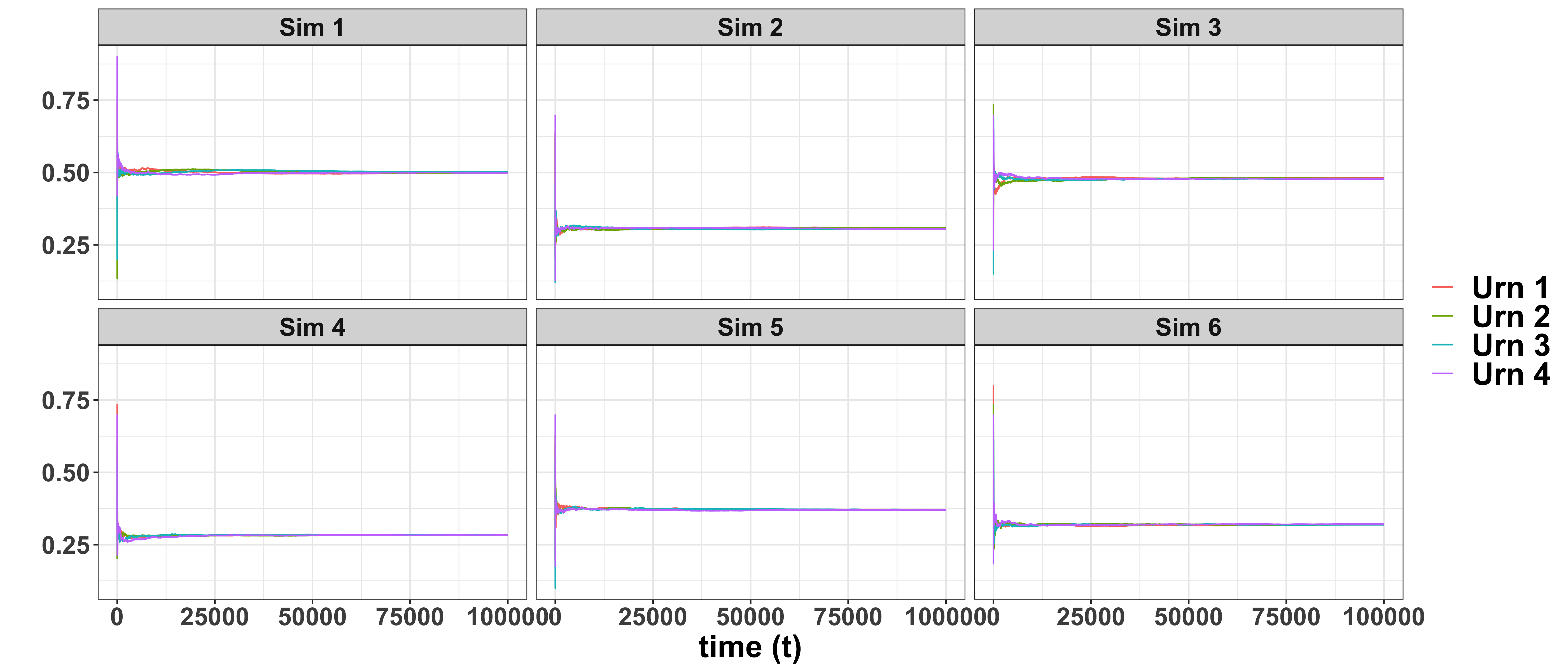
   Figure 5: Convergence of $Z^{t}_{1},\dots,Z_{4}^{t}$ in 6 different simulations.

   We first note that the graph in Figure 4 does not satisfy conditions (i) and (ii) of Theorem 3.1, as all nodes are Pólya type and there is no stubborn node. However based on Algorithm 1 there is a valid graph partition and thus it does not satisfy condition (iii) of Theorem 3.1.

   This case corresponds to a specific instance of Pólya-type reinforcement at each node in a $d$-regular graph (where $d_{i}^{\mathrm{in}}=d_{i}^{\mathrm{out}}=d,\forall i)$ for $d=2$, which was earlier studied in [8]. In this work, authors showed that there is a synchronisation with a random limit, that is there exists a random variable $Z^{\infty}$ such that $\lim_{t\to\infty}\mbox{${\mathbf{Z}}$}^{t}=Z^{\infty}(1,1,1,1)$. The simulation results, depicted in Figure 5, also suggest that the proportion of balls of either colour synchronises to the same random limit across all urns.

2. Consider the case when all nodes are preferential except node 4 (see Figure 6), that is $\mbox{${\mathcal{I}}$}=\mathop{\mathrm{Diag}}(1,1,1,-1)$. We observe that this case satisfies condition (iii) of the Theorem 3.1, as it does not have a valid graph partition. Thus by Theorem 3.1, $\mbox{${\mathbf{Z}}$}^{t}$ has a deterministic limit, which is independent of the initial vector $\mbox{${\mathbf{Z}}$}^{0}$. Figure 7 and Figure 8 illustrate the convergence to a deterministic limit and also show that the $\mathop{\mathrm{Var}}(Z_{i}^{t})$ converges to zero for every $i=1,2,3,4$.

   Figure 6: A graph with 4 nodes with $\mbox{${\mathcal{P}}$}=\{1,2,3\},\mbox{${\mathcal{D}}$}=\{4\}$.

   

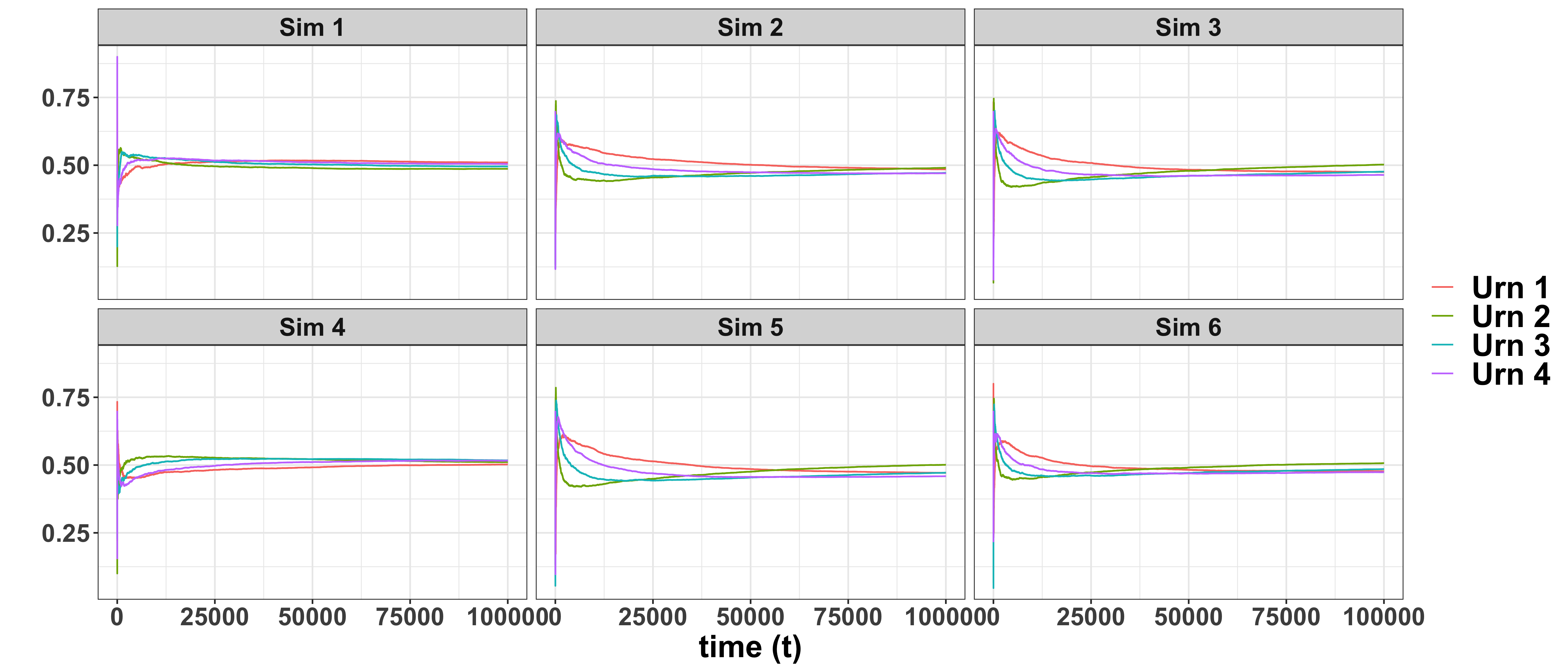
   Figure 7: Convergence of $Z^{t}_{1},\dots,Z_{4}^{t}$ in 6 different simulations. In this case, the limit is deterministic 0.5 for all urns.

   

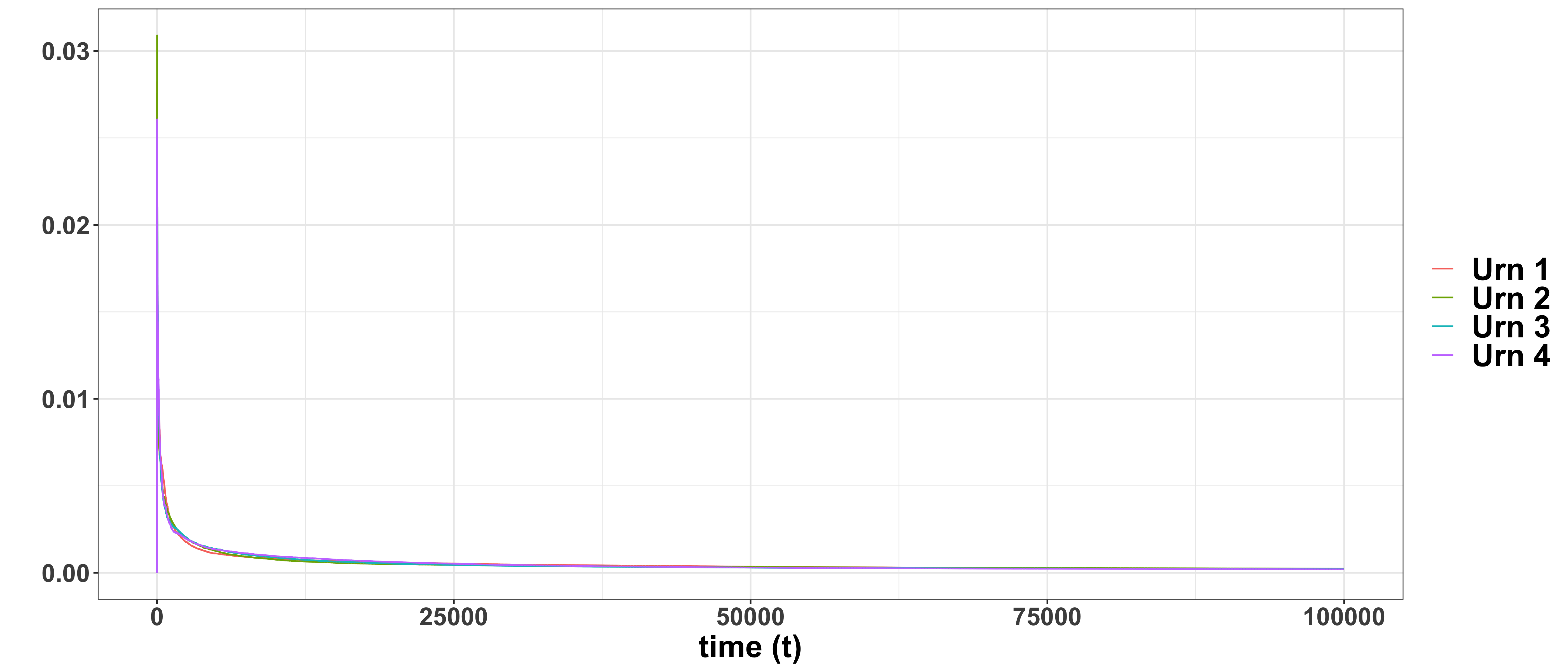
   Figure 8: Variance of $Z_{i}^{t}$ using 100 simulations converges to 0 as $t$ increases.

   Note that, in this case, the eigenvalues of the matrix $I-\mbox{${\mathbf{W}}$}$ are $1+\frac{1}{\sqrt{2}}+\frac{i}{\sqrt{2}},1+\frac{1}{\sqrt{2}}-\frac{i}{\sqrt{2}},1-\frac{1}{\sqrt{2}}+\frac{i}{\sqrt{2}},1-\frac{1}{\sqrt{2}}-\frac{i}{\sqrt{2}}$. Therefore $\rho=1-\frac{1}{\sqrt{2}}<1/2$ and $\Re(\lambda_{max})=\frac{1}{\sqrt{2}}$ and thus from (30) we get $\mathop{\mathrm{Var}}(\mbox{${\mathbf{Z}}$}^{t})\preccurlyeq t^{\sqrt{2}-2}$.

3. Now, we consider the case when all nodes are Pólya type and alternate nodes are de-preferential (see Figure  9), that is $\mbox{${\mathcal{I}}$}=\mathop{\mathrm{Diag}}(1,1,-1,-1)$.

   Figure 9: A graph with 4 nodes with $\mbox{${\mathcal{P}}$}=\{1,2\},\mbox{${\mathcal{D}}$}=\{3,4\}$.

   Note that, the graph in Figure 9 has a valid graph partition as described in Algorithm 1 and thus does not satisfy any of the condition (i)–(iii) of Theorem 3.1. The simulation results in Figure 10 show that the limit in this case is random. Furthermore, the simulations suggest that the limit takes the form $\left(Z^{\infty},(1-Z^{\infty}),(1-Z^{\infty}),Z^{\infty}\right)$.

   

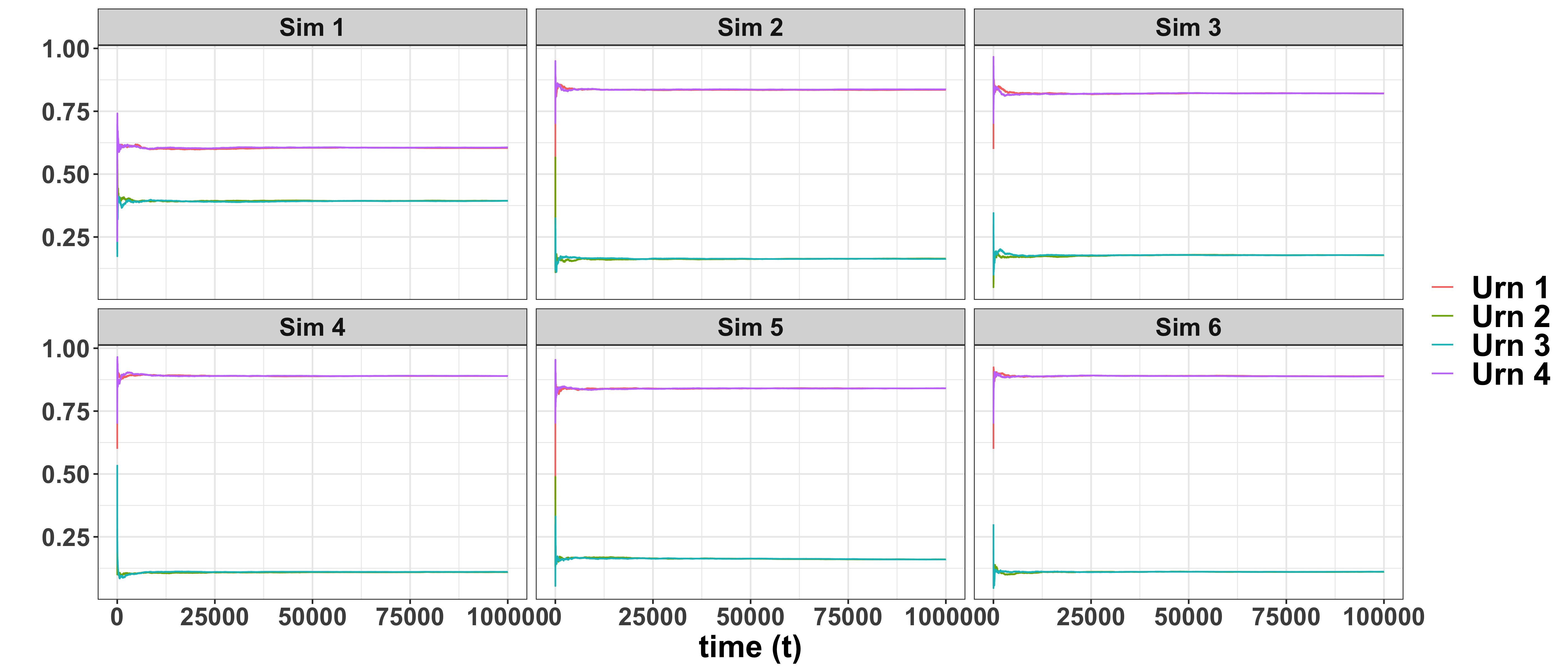
   Figure 10: Convergence of $Z^{t}_{1},\dots,Z_{4}^{t}$ in 6 different simulations.

   

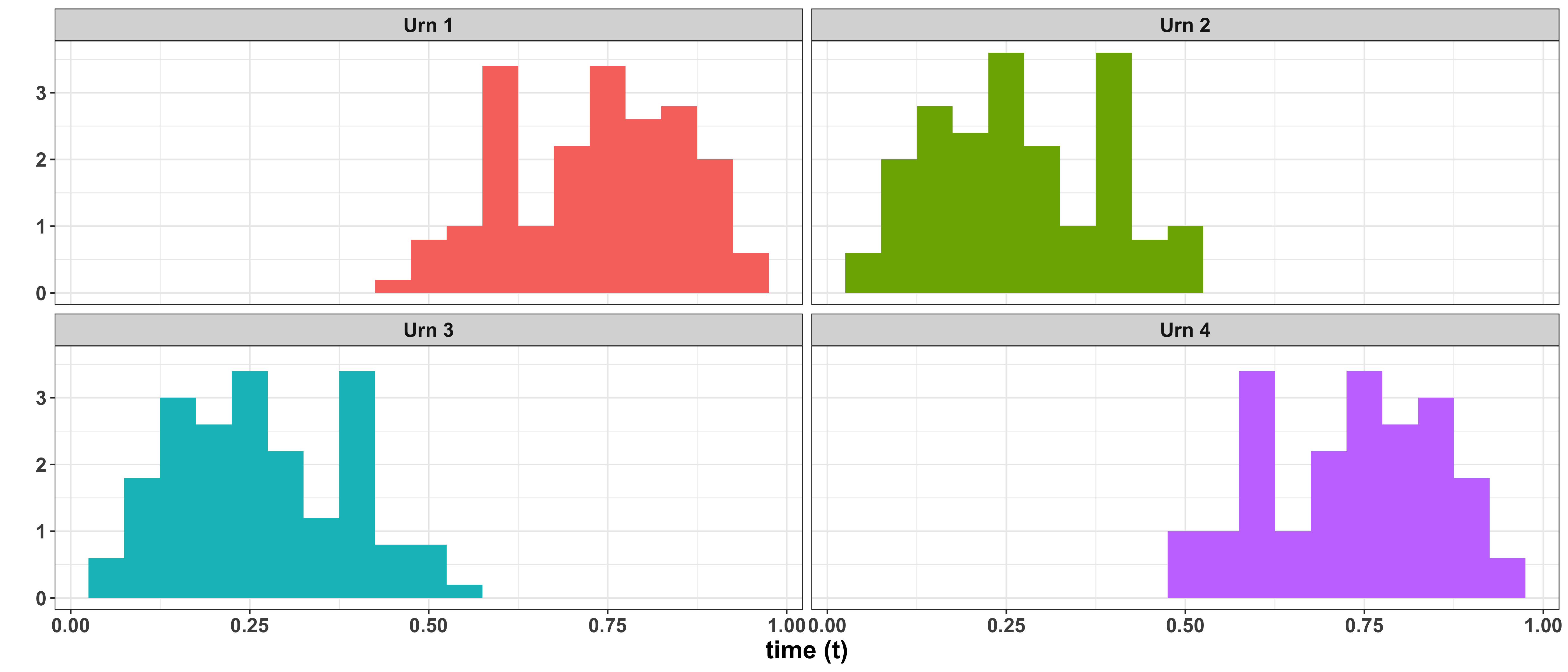
   Figure 11: Histogram of $Z^{t}_{i}$ in 100 different simulations, at $t=100000$, for the 4 interacting urns placed on the nodes of the graph as in Figure 9.

5.2 Discussion

For a graph that can be partitioned using Algorithm 1, the fraction of balls of either colour in each urn converges to a random limit. Specifically, from our simulations, we conjecture that in a cycle graph with alternating preferential and de-preferential nodes, the limiting behavior results in the fractions of balls of either colour in $P_{1},D_{2}$ (or $P_{2},D_{1}$) converging to the same limit almost surely. Further analysis of these cases is left as future work.

References

- [1] Aletti, G., Crimaldi, I. and Ghiglietti, A. (2017). Synchronization of reinforced stochastic processes with a network-based interaction. Ann. Appl. Probab. 27, 3787–3844.
- [2] Aletti, G. and Ghiglietti, A. (2017). Interacting generalized friedman’s urn systems. Stochastic Processes and their Applications 127, 2650–2678.
- [3] Bandyopadhyay, A. and Kaur, G. (2018). Linear de-preferential urn models. Adv. in Appl. Probab. 50, 1176–1192.
- [4] Borkar, V. S. (2008). Stochastic approximation. Cambridge University Press, Cambridge; Hindustan Book Agency, New Delhi. A dynamical systems viewpoint.
- [5] Crimaldi, I., Dai Pra, P. and Minelli, I. G. (2016). Fluctuation theorems for synchronization of interacting pólya’s urns. Stochastic processes and their applications 126, 930–947.
- [6] D., Y. and Sahasrabudhe, N. Urns with multiple drawings and graph-based interaction 2023.
- [7] Kaur, G. (2019). Negatively reinforced balanced urn schemes. Adv. in Appl. Math. 105, 48–82.
- [8] Kaur, G. and Sahasrabudhe, N. (2023). Interacting urns on a finite directed graph. J. Appl. Probab. 60, 166–188.
- [9] Mahmoud, H. M. (2009). Pólya urn models. Texts in Statistical Science Series. CRC Press, Boca Raton, FL.
- [10] Sahasrabudhe, N. (2016). Synchronization and fluctuation theorems for interacting Friedman urns. J. Appl. Probab. 53, 1221–1239.
- [11] Zhang, L.-X. (2016). Central limit theorems of a recursive stochastic algorithm with applications to adaptive designs. Ann. Appl. Probab. 26, 3630–3658.