Learning Feynman integrals from differential equations with neural networks

Abstract

We present a new approach for evaluating Feynman integrals numerically. We apply the recently-proposed framework of physics-informed deep learning to train neural networks to approximate the solution to the differential equations satisfied by the Feynman integrals. This approach relies neither on a canonical form of the differential equations, which is often a bottleneck for the analytical techniques, nor on the availability of a large dataset, and after training yields essentially instantaneous evaluation times. We provide a proof-of-concept implementation within the PyTorch framework, and apply it to a number of one- and two-loop examples, achieving a mean magnitude of relative difference of around 1% at two loops in the physical phase space with network training times on the order of an hour on a laptop GPU.

1 Introduction

The importance of Feynman integrals in theoretical physics can hardly be overstated. They play a central role in quantum field theory, where they are necessary to obtain precise predictions for collider phenomenology and to unveil fundamental properties of the theory, but also find application in a growing range of other fields, such as gravitational waves, cosmology and statistical mechanics. Their analytic expressions sport an intriguing ‘bestiary’ of special functions, which has sparked the interest of mathematicians and has led to a fruitful cross-contamination between mathematics and physics.

The interest for Feynman integrals is therefore growing, and so is the effort in the search for techniques for evaluating them. One of the most powerful approaches is the method of differential equations Barucchi:1973zm ; Kotikov:1990kg ; Kotikov:1991hm ; Gehrmann:1999as ; Bern:1993kr ; Henn:2013pwa , in which Feynman integrals are viewed as solutions to certain DEs. Solving these DEs analytically in terms of well-understood classes of special functions guarantees efficient numerical evaluation and complete analytical control, but is not always feasible. In such cases, one may resort to a numerical solution of the DEs. In particular, the numerical solution through series expansions is gaining increasing interest after this technique was generalised from the univariate Pozzorini:2005ff ; Aglietti:2007as ; Lee:2017qql ; Lee:2018ojn ; Bonciani:2018uvv ; Fael:2021kyg ; Fael:2022rgm to the multivariate case Liu:2017jxz ; Moriello:2019yhu ; Hidding:2020ytt ; Liu:2021wks ; Liu:2022chg ; Armadillo:2022ugh . The most widely used fully numerical method is Monte Carlo integration with sector decomposition Binoth:2000ps ; Bogner:2007cr ; Kaneko:2009qx ; Borowka:2012yc ; Borowka:2015mxa ; Borowka:2017idc ; Borowka:2018goh ; Heinrich:2023til ; Smirnov:2008py ; Smirnov:2009pb ; Smirnov:2013eza ; Smirnov:2015mct ; Smirnov:2021rhf . In addition to these, the long interest for Feynman integrals has led to a wide collection of other methods, such as Mellin-Barnes representation Usyukina:1992jd ; Usyukina:1993ch ; Smirnov:1999gc ; Tausk:1999vh ; Czakon:2005rk ; Smirnov:2009up ; Gluza:2007rt ; Belitsky:2022gba , recurrence relations Tarasov:1996br ; Lee:2009dh ; Lee:2012te , symbolic integration Brown:2008um ; Panzer:2014caa , loop-tree duality Catani:2008xa ; Runkel:2019yrs ; Capatti:2019ypt , Monte Carlo integration with tropical sampling Borinsky:2020rqs ; Borinsky:2023jdv , and positivity constraints Zeng:2023jek . We refer the interested readers to the comprehensive reviews Smirnov:2012gma ; Weinzierl:2022eaz . Recently, a few studies are beginning to explore the possibility of employing machine-learning methods in the evaluation of Feynman integrals. In ref. Winterhalder:2021ngy , the authors use a neural network (NN) to optimise the choice of integration contour to optimise the Monte Carlo integration with sector decomposition. Another approach consists in training a NN to learn the primitive of an integral, then replacing the Monte Carlo integration with evaluations of the primitive Maitre:2022xle ; Cruz-Martinez:2023vgs . A compendium of machine-learning applications in particle physics is available in refs. Feickert:2021ajf ; Butter:2022rso ; hepmllivingreview .

In this paper we propose a new avenue: using machine learning to solve the DEs numerically. We use deep NNs as universal function approximators HORNIK1989359 , and train them to approximate the solution to the DEs by minimising a loss function that includes the DEs themselves along with a set of boundary values. We build on the recently-proposed framework of physics-informed deep learning (PIDL) raissi2017physicsI ; raissi2017physicsII ; raissi2019physics . In contrast to the traditional machine learning regime, where one trains on a large dataset, here we use a small dataset — the boundary values for the DEs — and strong physical constraints in the form of DEs. A preliminary application of this method to Feynman integrals was studied by one of the authors in his bachelor’s thesis project thesis-calisto . This approach is very flexible as it does not rely on a canonical form of the DEs Henn:2013pwa , unlike the analytical techniques, and after training yields essentially instantaneous evaluation times, unlike the numerical methods, at the cost of a lower control over the precision.

In addition to discussing our new approach, we provide a proof-of-concept implementation repo ; zenodo within the PyTorch framework paszke2019pytorch , along with a number of one- and two-loop examples models ; zenodo , some of them at the cutting edge of our current computational capabilities. For these, we achieved a mean magnitude of relative difference of order 1% at two loops in testing over the physical phase space, with NN training times on the order of an hour on a laptop GPU.

This article is organised as follows. In section 2, we review the method of DEs for calculating Feynman integrals. In section 3, we describe how we apply PIDL to solve those DEs. In section 4, we present example applications of our method to several integral families. We conclude in section 5. Appendix A collects the definitions of the integral families considered in this work.

2 Differential equations for Feynman integrals

In this section, we give a quick overview of the method of DEs for computing Feynman integrals Barucchi:1973zm ; Kotikov:1990kg ; Kotikov:1991hm ; Gehrmann:1999as ; Bern:1993kr ; Henn:2013pwa . In this approach, the problem of loop integration is traded for that of solving a system of first-order partial differential equations of the form

$$\frac{\partial}{\partial v_{i}}\vec{F}(\vec{v};\epsilon)=A_{v_{i}}(\vec{v};\epsilon)\cdot\vec{F}(\vec{v};\epsilon)\,,\qquad\forall\,i=1,\ldots,{n_{v}}\,,$$ (1)

where $\vec{F}=(F_{1},\ldots,F_{n_{F}})$ is an array of ${n_{F}}$ Feynman integrals, $\vec{v}=(v_{1},\ldots,v_{{n_{v}}})$ are the ${n_{v}}$ independent kinematic variables, and $\epsilon=(4-d)/2$ in $d$ spacetime dimensions. The entries of the connection matrices $A_{v_{i}}$ in eq. 1 are functions of $\vec{v}$ and $\epsilon$. The DEs are complemented by (at least) one set of values $\vec{F}(\vec{v}_{0};\epsilon)$ at an arbitrary phase-space point $\vec{v}_{0}$, which serves as the boundary condition. We are interested in the Laurent expansion of the solution to the PDEs in eq. 1 around $\epsilon=0$,

$$\vec{F}(\vec{v};\epsilon)=\epsilon^{w^{*}}\sum_{w\geq 0}\epsilon^{w}F^{(w)}(\vec{v})\,,$$ (2)

where $w^{*}$ is typically $-2\ell$ for an $\ell$-loop integral family. We will truncate the expansion at some order $w_{\rm max}$ depending on the intended application.

In section 2.1 we will show how the DEs can be derived for a given family of Feynman integrals using an explicit toy example. The readers who are already familiar with this method may go directly to section 2.2, which is devoted to a general characterisation of the DEs addressed in this work. In section 2.3 we list a number of properties of the DEs and of their solutions which will be important for this work.

2.1 Warm up: the massless box

In this section, we derive the DEs for the one-loop four-point “massless box” Feynman integrals. A more pedagogical discussion of this example can be found e.g. in refs. Henn:2014qga ; Badger:2023eqz .

An integral family is the set of all scalar integrals with a given propagator structure. The integrals of the massless box family are defined as

$$\mathrm{I}_{\vec{a}}(s,t;\epsilon)=\int\frac{\text{d}^{d}k}{\mathrm{i}\pi^{d/2}}\frac{\mu^{4-d}}{D_{1}^{a_{1}}D_{2}^{a_{2}}D_{3}^{a_{3}}D_{4}^{a_{4}}}\,,$$ (3)

where $\mu$ is the dimensional regularisation scale, $\vec{a}=(a_{1},a_{2},a_{3},a_{4})\in\mathbb{Z}^{4}$, and $D_{i}$ are the inverse propagators associated with the graph in figure 1:

Figure 1: Graph representing the propagator structure of the massless box integral family. The arrows denote the directions of the momenta.

$$\begin{aligned} D_{1}&=-k^{2}-\mathrm{i}0^{+}\,,\qquad\qquad&&D_{3}=-(k+p_{1}+p_{2})^{2}-\mathrm{i}0^{+}\,,\\ D_{2}&=-(k+p_{1})^{2}-\mathrm{i}0^{+}\,,\qquad\qquad&&D_{4}=-(k-p_{4})^{2}-\mathrm{i}0^{+}\,,\end{aligned}$$ (4)

with $0^{+}$ a positive infinitesimal. We set $\mu=1$; the dependence on it can be recovered from dimensional analysis. The external momenta $p_{i}$ are taken to be outgoing, and satisfy momentum conservation and on-shell conditions:

$$\sum_{i=1}^{4}p_{i}=0\,,\qquad\qquad p_{i}^{2}=0\quad\forall\,i=1,\ldots,4\,.$$ (5)

We choose the two independent Lorentz invariants as $s=(p_{1}+p_{2})^{2}$ and $t=(p_{2}+p_{3})^{2}$.

Within each family only finitely many integrals are linearly independent. They are called master integrals, and constitute a basis of the family. Any integral of the family can thus be “reduced” to a linear combination of MIs. The coefficients are rational functions of the kinematic invariants and $\epsilon$. The standard way to determine the MIs and reduce to MIs is to solve systems of integration-by-parts (IBP) relations Tkachov:1981wb ; Chetyrkin:1981qh — linear relations among the integrals of a family — using the Laporta algorithm Laporta:2000dsw . We generate the required IBP relations using LiteRed Lee:2012cn , and solve them using FiniteFlow Peraro:2019svx . The box family has three MIs. Following the Laporta algorithm, they are chosen as

$$\vec{F}(s,t;\epsilon)=\begin{pmatrix}\mathrm{I}_{0,1,0,1}(s,t;\epsilon)\,,&\mathrm{I}_{1,0,1,0}(s,t;\epsilon)\,,&\mathrm{I}_{1,1,1,1}(s,t;\epsilon)\end{pmatrix}^{\top}\,.$$ (6)

We stress that the choice of MIs is arbitrary, provided they are linearly independent.

The derivatives of the MIs with respect to the kinematic invariants can be expressed as linear combinations of scalar integrals in the same family, and can thus be IBP-reduced to MIs themselves. As a result, we obtain a system of first-order PDEs:

$$\frac{\partial}{\partial s}\vec{F}(s,t;\epsilon)=\begin{pmatrix}0&0&0\\ 0&-\frac{\epsilon}{s}&0\\ \frac{2(2\epsilon-1)}{st(s+t)}&\frac{2(1-2\epsilon)}{s^{2}(s+t)}&-\frac{s+t+\epsilon\,t}{s(s+t)}\\ \end{pmatrix}\cdot\vec{F}(s,t;\epsilon)\,,$$ (7)

and similarly for $t$.

We are interested in the Laurent expansion of the solution around $\epsilon=0$,

$$\vec{F}(s,t;\epsilon)=\frac{1}{\epsilon^{2}}\sum_{k\geq 0}\epsilon^{k}\,\vec{F}^{(k)}(s,t)\,,$$ (8)

truncated at a certain order in $\epsilon$. To this end, the standard approach consists in looking for a MI basis such that the DEs simplify. For example, choosing

$$\vec{F}(s,t;\epsilon)=\begin{pmatrix}s\,t\,\mathrm{I}_{1,1,1,1}(s,t;\epsilon)\,,&s\,\mathrm{I}_{1,1,1,0}(s,t;\epsilon)\,,&t\,\mathrm{I}_{1,1,0,1}(s,t;\epsilon)\end{pmatrix}^{\top}$$ (9)

as MIs for the massless box family leads to DEs of the form

$$\frac{\partial}{\partial s}\vec{F}(s,t;\epsilon)=\epsilon\,A_{s}(s,t)\cdot\vec{F}(s,t;\epsilon)\,,$$ (10)

with

$$A_{s}(s,t)=\begin{pmatrix}\frac{1}{s+t}-\frac{1}{s}&\frac{2}{s+t}-\frac{2}{s}&\frac{2}{s+t}\\ 0&-\frac{1}{s}&0\\ 0&0&0\\ \end{pmatrix}\,,$$ (11)

and similarly for $t$. The DEs in eq. 10 are in the so-called canonical form Henn:2013pwa : the connection matrices depend on $\epsilon$ only through an overall factor and have at most simple poles at all singular loci. The factorisation of $\epsilon$ allows for an iterative solution of the DEs order by order in $\epsilon$. Plugging the Laurent expansion of eq. 8 into eq. 10 in fact gives the recursion

$$\frac{\partial}{\partial s}\vec{F}^{(k)}(s,t)=A_{s}(s,t)\cdot\vec{F}^{(k-1)}(s,t)\,,$$ (12)

for $k\geq 1$, starting from $\vec{F}^{(0)}(s,t)$ which is constant. If the connection matrices are rational functions, the solution can be written algorithmically in terms of multiple polylogarithms up to any order in $\epsilon$. The boundary values can be determined by evaluating the MIs numerically, or by imposing physical consistency conditions (see refs. Henn:2014qga ; Badger:2023eqz ). For example, for the first MI in eq. 9 we obtain

$$\begin{aligned} F_{1}(s,t;\epsilon)=\,&\frac{\mathrm{e}^{-\epsilon\gamma_{\rm E}}(-s)^{-\epsilon}}{\epsilon^{2}}\biggl{\{}4-2\epsilon\log\left(\frac{t}{s}\right)-\frac{4}{3}\pi^{2}\epsilon^{2}+\epsilon^{3}\biggl{[}2\,\mathrm{Li}_{3}\left(-\frac{t}{s}\right)\\ &-2\log\left(\frac{t}{s}\right)\mathrm{Li}_{2}\left(-\frac{t}{s}\right)-\log^{2}\left(\frac{t}{s}\right)\log\left(\frac{s+t}{t}\right)+\frac{1}{3}\log^{3}\left(\frac{t}{s}\right)\\ &+\frac{7}{6}\pi^{2}\log\left(\frac{t}{s}\right)-\pi^{2}\log\left(\frac{s+t}{s}\right)-\frac{34}{3}\zeta_{3}\biggr{]}+\mathcal{O}\left(\epsilon^{4}\right)\biggr{\}}\,,\end{aligned}$$ (13)

where ${\rm Li}_{n}$ is the weight-$n$ classical polylogarithm, $\zeta_{n}$ is the Riemann zeta constant, and $\gamma_{\rm E}$ is the Euler-Mascheroni constant.

2.2 General form of the differential equations

In the previous section, we have seen that finding a MI basis that satisfies canonical DEs simplifies the solution substantially. This is however a difficult endeavour, for which no general algorithm exists. What is more, special functions that are more complicated than MPLs may be required to express the solution analytically (see e.g. ref. Bourjaily:2022bwx for a recent review). The notion of “canonical” DEs in such cases is still object of ongoing research, and the mathematical technology to handle the relevant special functions is far from being ripe.

Our approach does not rely on the canonical form of the DEs, and is insensitive to the class of special functions involved in the solution. We will make only the following mild assumptions about the connection matrices $A_{v_{i}}(\vec{v};\epsilon)$ in eq. 1. We will assume that:

1. they are rational functions of the kinematic variables $\vec{v}$ and $\epsilon$;

2. they are finite at $\epsilon=0$, and can thus be expanded as

   $$A_{v_{i}}(\vec{v};\epsilon)=\sum_{k=0}^{k_{\rm max}}\epsilon^{k}A^{(k)}_{v_{i}}(\vec{v})\,,$$ (14)

   where $k_{\rm max}$ is either a positive integer or infinity.

We stress that both these assumptions are in principle not necessary for our method, but are useful simplifications.

The first condition is easy to achieve. Square roots or more complicated functions in fact appear in the connection matrices only if they are present in the definition of the MIs. If the latter contain only rational functions, as in eq. 9 for the massless box family, the connection matrices are guaranteed to be rational. This condition implies that the connection matrices are real-valued for real kinematic variables $\vec{v}$, which allows us to decouple the real and imaginary parts of the MIs. The latter satisfy the same DEs,

$$\frac{\partial}{\partial v_{i}}\mathrm{Re}\left[\vec{F}(\vec{v};\epsilon)\right]=A_{v_{i}}(\vec{v};\epsilon)\cdot\mathrm{Re}\left[\vec{F}(\vec{v};\epsilon)\right]\,,$$ (15)

$$\frac{\partial}{\partial v_{i}}\mathrm{Im}\left[\vec{F}(\vec{v};\epsilon)\right]=A_{v_{i}}(\vec{v};\epsilon)\cdot\mathrm{Im}\left[\vec{F}(\vec{v};\epsilon)\right]\,,$$ (16)

though with different boundary values. Furthermore, this assumption allows us to avoid any operations with complex numbers, making the implementation simpler and more efficient.

The construction of a MI basis which satisfies the second condition is less trivial (see e.g. refs. Lee:2019wwn ; Dubovyk:2022frj ), but is substantially simpler than obtaining a canonical form. For the most complicated family computed in this paper, for instance, it simply amounted to choosing the MIs according to the algorithm of ref. Smirnov:2020quc ; Usovitsch:2020jrk , and normalising some of them by suitable factors of $\epsilon$. We will discuss how we achieved this for each of the examples in section 4. The advantage of this form of the connection matrices is that it leads to a recursive structure of the solution where the coefficients of the $\epsilon$-expansion of the MIs in eq. 2 are coupled by the DEs only to themselves and to lower-order coefficients:

$$\frac{\partial}{\partial v_{i}}\vec{F}^{(w)}(\vec{v})=\sum_{k=0}^{\mathrm{min}(w,k_{\rm max})}A^{(k)}_{v_{i}}(\vec{v})\cdot\vec{F}^{(w-k)}(\vec{v})\,.$$ (17)

While our method works in principle for any $k_{\rm max}$, low values are preferable. It is therefore worth putting some effort into reducing $k_{\rm max}$. Moreover, since we are interested in the solution only up to a certain order, say $w_{\rm max}$, the terms of the connection matrices of order greater than $w_{\rm max}$ do not contribute.

In conclusion, we will solve systems of PDEs of the form

$$\frac{\partial}{\partial v_{i}}\vec{G}^{(w)}(\vec{v})=\sum_{k=0}^{\mathrm{min}(w,k_{\rm max})}A^{(k)}_{v_{i}}(\vec{v})\cdot\vec{G}^{(w-k)}(\vec{v})\,,\qquad\forall\ i=1,\ldots,{n_{v}}\,,$$ (18)

from $w=0$ up to a given order, complemented by (at least) one set of boundary values $\vec{G}^{(w)}(\vec{v}_{0})$ obtained by evaluating numerically the MIs. Here, $\vec{G}^{(w)}(\vec{v})$ is either the real or the imaginary part of the MI coefficients $\vec{F}^{(w)}(\vec{v})$, and the entries of the connection matrices $A^{(k)}_{v_{i}}(\vec{v})$ are rational functions of the kinematic variables $\vec{v}$.

2.3 Properties of the differential equations

In this section, we collect a number of properties of the MIs and of the corresponding DEs, which will play a role in our machine learning approach to the solution.

Homogeneity

We choose the kinematic variables $\vec{v}$ as either scalar products $(p_{i}+p_{j})^{2}$ or squared masses $m_{i}^{2}$. The MIs are then homogeneous functions of $\vec{v}$, i.e. they satisfy the scaling condition

$${F}_{i}(\alpha\,\vec{v};\epsilon)=\alpha^{\lambda_{i}}{F}_{i}(\vec{v};\epsilon)\,,$$ (19)

for any positive factor $\alpha$, where the scaling dimensions $\lambda_{i}$ can be determined by dimensional analysis. The scaling in eq. 19 can be used to set one variable to a constant. We can for instance “freeze” the last variable $v_{{n_{v}}}$ to a constant $c_{{n_{v}}}$ by choosing $\alpha=c_{{n_{v}}}/v_{{n_{v}}}$ in eq. 19, obtaining

$${F}_{i}(\vec{v};\epsilon)=\left(\frac{v_{{n_{v}}}}{c_{{n_{v}}}}\right)^{\lambda_{i}}\,{F}_{i}\left(c_{{n_{v}}}\frac{v_{1}}{v_{{n_{v}}}},\ldots,c_{{n_{v}}}\frac{v_{{n_{v}}-1}}{v_{{n_{v}}}},c_{{n_{v}}};\epsilon\right)\,.$$ (20)

This allows us to treat the integrals as functions of ${n_{v}}-1$ ratios. The choice of which variable to freeze and of which value to fix it to both have an impact on the NN fit. Similarly, it is sometimes convenient to choose the MIs so that their scaling dimensions $\lambda_{i}$ in eq. 19 are all zero. We will discuss these aspects in section 3.

Singularities

The denominators of the connection matrices encode the singularity structure of the solution to the DEs. In other words, the solution to the DEs may be singular where any of the denominator factors of the connection matrices vanishes. We distinguish between spurious and physical singularities. On a spurious singularity, the connection matrices are singular while the solution stays finite. On a physical singularity, instead, also the solution is singular. For the massless box integrals discussed in section 2.1, for example, the denominator factors of the DEs are $\{s,t,s+t\}$. Of these, $s=0$ and $t=0$ are physical singularities, while $s+t=0$ is spurious.

Multivaluedness

Feynman integrals, and hence the special functions appearing in them, are multivalued functions. Care must be taken that they are evaluated on the correct branch. The expression for the box integral in eq. 13 is for instance well-defined in the Euclidean region ($s<0\land t<0$). Some work is required to analytically continue it to the physical region of interest for phenomenology ($s>0\land t<0$). We sidestep this problem by working always within a given kinematic region, never crossing its borders into another one. In practice, this means that we choose boundary points in the chosen region, and fit the solution to the DEs in that region only. This way the boundary values instruct the NN which branch of the solution to fit, and no explicit analytic continuation is required.

3 Deep learning Feynman integrals

In this section, we detail our application of machine learning techniques to solving Feynman integrals from their DEs. Note that all hyperparameters are selected manually without extensive optimisation, this being an exploratory study.

In brief, NNs are trained by minimising a heuristic that we call the loss function, typically using a variant of stochastic gradient descent Goodfellow-et-al-2016 . By evaluating the loss function and then considering its derivatives with respect to the parameters of the NN, we can adjust those parameters to reduce the value of the loss function. Repeating this iteratively, we converge on a minimum of the loss function. The derivatives of the loss function are generally computed using an algorithmic method called automatic differentiation doi:10.1137/1.9780898717761 .

This machinery can be used for regression analysis, where the NN becomes a function approximator. Say we wish to emulate a target function $g$ with a NN surrogate $h$. If we have a large dataset of $N$ values of the target at points $x^{(i)}$,

$$\mathrm{D}\coloneqq\left\{\left(x^{(i)},g\bigl{(}x^{(i)}\bigr{)}\right)\,\Bigl{|}\,i=1,\ldots,N\right\}\,,$$ (21)

we can use a loss function $L(\mathrm{D},\theta)$ that compares this target distribution to the output of our NN, where $\theta$ are the parameters (weights and biases) of the NN. What constitutes a large $N$ depends on the number of input dimensions and the complexity of the target distribution. A common choice is the mean squared error loss function,

$$L(\mathrm{D},\theta) =\frac{1}{N}\sum_{i=1}^{N}\Bigl{[}h\bigl{(}x^{(i)};\theta\bigr{)}-g\bigl{(}x^{(i)}\bigr{)}\Bigr{]}^{2}\,.$$ (22)

For integral families of interest, we do not have access to a large dataset because generating sample points with existing evaluation methods is prohibitively slow, so this approach is unviable. However, we do know the DEs 18 and can cheaply numerically sample their connection matrices. Therefore, we can instead train a NN to satisfy the DEs by including in our loss function a soft constraint term which minimises the difference between the two sides of the DEs as estimated by the NN. To fully determine the solution, we also specify at least one set of boundary values as another constraint term in our loss function. This approach comes under the paradigm of physics-informed deep learning (PIDL) raissi2017physicsI ; raissi2017physicsII ; raissi2019physics ; we refer the interested reader to the tutorials navarro2023solving ; baty2023solving and recent reviews of related literature Karniadakis2021 ; cuomo2022scientific ; hao2023physicsinformed ; faroughi2023physicsguided .

Our application of PIDL is however somewhat peculiar. Usually, in the machine learning community, PIDL is used in architectures which blend data-driven and model-driven (i.e., physics-informed) components. The role of the latter is to constrain the network to physically sensible results (for instance, by imposing energy conservation), while the remaining part of the learning is still performed using a data-driven loss function. In that setting, PIDL contributes to the “physics for machine learning” cause. On the contrary, we limit the data-driven part to a few boundary conditions and leave the bulk of learning to be model-driven, as the DEs themselves represent, perturbatively, an exact solution to the problem. Ours is therefore an instance of the “machine learning for physics” cause.

This section is organised as follows. In section 3.1, we discuss the architecture of our model. In section 3.2, we detail the datasets and the subtleties of their creation. In section 3.3, we define our loss function. In section 3.4, we describe the training procedure. Finally, in section 3.5, we cover the uncertainty and error analysis.

3.1 Model architecture

Figure 2: Architecture of the NN with outputs $h_{i}^{(w)}(\vec{x})$ to fit the MI coefficients $g_{i}^{(w)}(\vec{x})$ as described in section 3.1. The input nodes are shown in green, the hidden layer nodes in blue, and the output nodes in orange. In our applications, the number of output nodes is much larger than that of the input nodes.

We approximate the MI coefficients $\vec{F}^{(w)}(\vec{v})$ for $w=0,\ldots,w_{\rm max}$ with a model comprising a pair of fully-connected feedforward NNs. Each NN is a real-valued function, with one for the real and one for the imaginary parts of the MI coefficients, which we collectively refer to as $\vec{G}^{(w)}(\vec{v})$ as in eq. 18.

The NNs have ${n_{v}}-1$ inputs $\vec{x}\coloneqq(x_{1},\ldots,x_{{n_{v}}-1})$, which are related to a subset of the ${n_{v}}$ kinematic variables $\vec{v}$. We make use of the homogeneity of the solution (see section 2.3) to drop the dependence on one of the variables, as decreasing the input dimensionality reduces the complexity of the problem. The choice of which variable to freeze is made considering the kinematics of the particular family; for instance, natural choices include $s_{12}=(p_{1}+p_{2})^{2}$ for a massless system with incoming momenta $p_{1}$ and $p_{2}$, or the (squared) mass in a system with an internal mass. If we fix the last variable $v_{{n_{v}}}$ to a constant $c_{{n_{v}}}$ and define the variables

$$x_{i}\coloneqq c_{{n_{v}}}\frac{v_{i}}{v_{{n_{v}}}}\qquad\forall\,i=1,\ldots,{n_{v}}-1\,,$$ (23)

from eq. 20 — which holds separately at each order in $\epsilon$, and for both real and imaginary parts — it follows that

$$G_{i}^{(w)}(\vec{v})=\left(\frac{v_{{n_{v}}}}{c_{{n_{v}}}}\right)^{\lambda_{i}}g_{i}^{(w)}\left(x_{1},\ldots,x_{{n_{v}}-1}\right)\,,$$ (24)

where $g_{i}^{(w)}$ is a function of ${n_{v}}-1$ variables $\vec{x}$,

$$g_{i}^{(w)}(\vec{x})\coloneqq G_{i}^{(w)}(x_{1},\ldots,x_{{n_{v}}-1},c_{{n_{v}}})\,.$$ (25)

The sets of functions $\vec{g}^{(w)}(\vec{x})\coloneqq(g_{1}^{(w)},\ldots,g_{n_{F}}^{(w)})$ for $w=0,\ldots,w_{\rm max}$ then satisfy DEs of the same form as eq. 18 for the MI coefficients,

$$\frac{\partial}{\partial x_{i}}\vec{g}^{(w)}(\vec{x})=\sum_{k=0}^{\mathrm{min}(w,k_{\rm max})}A^{(k)}_{x_{i}}(\vec{x})\cdot\vec{g}^{(w-k)}(\vec{x})\,,$$ (26)

for $i=1,\ldots,{n_{v}}-1$ and $w=0,\ldots,w_{\rm max}$, with connection matrices $A^{(k)}_{x_{i}}(\vec{x})$ which can be derived from those in eq. 18 through the chain rule.

Our NNs are trained to fit the sets of functions $\vec{g}^{(w)}$ for $w$ from $0$ to $w_{\rm max}$, that is

$${n_{\epsilon}}\coloneqq w_{\rm max}+1$$ (27)

orders in $\epsilon$. The outputs of a NN correspond to the functions $g_{i}^{(w)}(\vec{x})$. Each NN thus has ${n_{F}}\,{n_{\epsilon}}$ outputs, which are typically many more than the inputs $\vec{x}$.

For the integral families we considered, we find that three or four hidden layers are sufficient. Validation performance saturates with square (constant width) configurations with a width of around double the number of outputs for three layers or similar to the number of outputs for four layers. The architecture of the NN is sketched in figure 2. The choice of activation functions is critical in PIDL wang2023learning ; we use gaussian error linear unit (GELU) activation functions hendrycks2023gaussian on the hidden layers, with a linear output layer. We use 32 bit floating point numbers, finding this numerical precision to not be a limiting factor of the training performance.

3.2 Datasets

The training dataset $\mathrm{D}$ has two subsets: a DE dataset $\mathrm{D}_{\rm DE}$ and a boundary dataset $\mathrm{D}_{\rm b}$. The DE dataset comprises a set of input points and the corresponding values of the connection matrices:

$$\mathrm{D}_{\rm DE}\coloneqq\left\{\left(\vec{x}^{(i)},A_{x_{j}}^{(k)}\bigl{(}\vec{x}^{(i)}\bigr{)}\right)\,\Bigl{|}\,i=1,\ldots\right\}\,.$$ (28)

Here, by $A_{x_{j}}^{(k)}\bigl{(}\vec{x}^{(i)}\bigr{)}$ we mean the set of connection matrices for all variables ($j=1,\ldots,{n_{v}}-1$) and at all the relevant orders in $\epsilon$ ($k=0,\ldots,k_{\rm max}$), evaluated at $\vec{x}^{(i)}$. The DE dataset is generated dynamically by random sampling at each iteration of the training algorithm (see section 3.4), while all other datasets are static and pre-computed. The boundary dataset contains input points with values of the solution,

$$\mathrm{D}_{\rm b}\coloneqq\left\{\left(\vec{x}^{(i)},\vec{g}^{(w)}\bigl{(}\vec{x}^{(i)}\bigr{)}\right)\,\Bigl{|}\,i=1,\ldots\right\}\,,$$ (29)

where $\vec{g}^{(w)}\bigl{(}\vec{x}^{(i)}\bigr{)}$ includes all required orders in $\epsilon$ ($w=0,\ldots,w_{\rm max}$). There is also another dataset of this form for testing. 64 bit floating point numbers are used to generate and store all datasets, with the exception of solution values computed with arbitrary-precision arithmetic by AMFlow Liu:2017jxz ; Liu:2021wks ; Liu:2022chg as noted in section 4.

As we anticipated in section 2.3, we target a single phase-space region, where the solution is single-valued, so that no analytic continuation needs to be performed. The phase-space points of all datasets are thus chosen within said region, and the fit is valid only there. The boundaries of the kinematic regions are physical singularities (both connection matrices and solution are singular), while the bulk of the phase space can be crossed by both physical and spurious singularities (the connection matrices are singular but the solution is finite). When sampling points for all datasets, we must thus place cuts around the physical singularities. Furthermore, for the DE dataset only, we must also cut the spurious poles to avoid divergences in the numerical evaluation of the connection matrices. We stress however that the NNs can be evaluated also in the regions surrounding the spurious singularities excluded from the DE dataset, and actually exhibit good accuracy there as well. We choose the cuts to be as small as possible while regulating the singular behaviour to minimise the absence of model exposure to these regions during training.

More concretely, we parametrise the phase space of the physical scattering region of interest in terms of energies and angles, then generate the points of the input space $\vec{x}$ for DE and testing datasets by random uniform sampling of the parametrisation. In addition, we veto points that do not pass the appropriate singularity cuts. This provides a simple sampling method for this exploratory study.

Stochastic gradient descent algorithms are highly sensitive to the range of magnitudes involved in the problem, training optimally when all scales are of the same order. In particular, large scale variations in the distributions of the inputs and outputs can be problematic. We select from two methods to ameliorate the output distribution, finding that the better option depends on the integral family:

• constructing integrals with null scaling dimensions (see eq. 19), including tuning the choice of prefactor used to normalise the integrals;

• using a judicious choice of the kinematic scaling $c_{{n_{v}}}$ in eq. 23 for integrals with non-zero scaling dimensions.

The choice of $c_{{n_{v}}}$ can also be exploited to adjust the input distribution and shift the spurious surfaces such that the spurious cuts exclude less of the physical region. Cumulatively, these choices can have a significant impact on training performance and must be fine tuned.

While it is sufficient to specify a single boundary point, we find that training performance can be improved by including additional points in the boundary dataset. The optimal configuration depends on the specific system, but we note some trends. For small boundary datasets, we find that points on the phase-space boundaries (including physical and spurious cuts) are more important than those in the interior, while having a mix of both becomes beneficial as the dataset size increases. If using random sampling of the interior, the significance of points on the boundary decreases with dataset size as more interior points randomly land near the boundaries. Performance generally increases with the total number of points, although the improvement diminishes as the size becomes very large. It is vital to choose points that well represent the scattering region, including coverage of the boundaries; we find that large randomly generated sets with many overlapping points can even perform worse than smaller ones with a more even distribution, for instance.

3.3 Loss function

We define the loss function $L(\mathrm{D},\theta)$ for a NN with outputs $\vec{h}^{(w)}(\vec{x};\theta)$ fitting a target solution $\vec{g}^{(w)}(\vec{x})$ for inputs $\vec{x}$. We write it as a sum of terms for the DEs ($L_{\rm DE}$) and for the boundary values ($L_{\rm b}$), using mean squared error for each term. Using the short-hand

$$\underset{i\in A}{\overset{}{\overline{\sum}}}\coloneqq\frac{1}{|A|}\sum_{i\in A}\ ,$$ (30)

with $|A|$ the cardinality of the set $A$, the DE terms of the loss function are

$$\begin{aligned} &L_{\rm DE}(\mathrm{D}_{\rm DE},\theta)=\\ &\qquad\underset{\vec{x}^{(i)}\in\mathrm{D}_{\rm DE}}{\overset{}{\overline{\sum}}}\,\underset{j=1}{\overset{{n_{F}}}{\overline{\sum}}}\underset{l=1}{\overset{{n_{v}}-1}{\overline{\sum}}}\underset{w=0}{\overset{w_{\rm max}}{\overline{\sum}}}\Biggl{[}\partial_{x_{l}}h_{j}^{(w)}\bigl{(}\vec{x}^{(i)};\theta\bigr{)}-\sum_{k=0}^{\min(w,k_{\rm max})}\sum_{r=1}^{{n_{F}}}A_{x_{l},jr}^{(k)}\bigl{(}\vec{x}^{(i)}\bigr{)}\,h_{r}^{(w-k)}\bigl{(}\vec{x}^{(i)};\theta\bigr{)}\Biggr{]}^{2}\,,\end{aligned}$$ (31)

while the boundary terms are given by

$$L_{\rm b}(\mathrm{D}_{\rm b},\theta) =\underset{\vec{x}^{(i)}\in\mathrm{D}_{\rm b}}{\overset{}{\overline{\sum}}}\,\underset{j=1}{\overset{{n_{F}}}{\overline{\sum}}}\underset{w=0}{\overset{w_{\rm max}}{\overline{\sum}}}\left[h_{j}^{(w)}\bigl{(}\vec{x}^{(i)};\theta\bigr{)}-g_{j}^{(w)}\bigl{(}\vec{x}^{(i)}\bigr{)}\right]^{2}\,.$$ (32)

We sum them to obtain the full loss function,

$$L(\mathrm{D},\theta)=L_{\rm DE}(\mathrm{D}_{\rm DE},\theta)+L_{\rm b}(\mathrm{D}_{\rm b},\theta)\,.$$ (33)

We recall that $\mathrm{D}\coloneqq\mathrm{D}_{\rm DE}\cup\mathrm{D}_{\rm b}$ is the training dataset defined in eqs. 28 and 29, $\theta$ are the parameters of the NN, and $A^{(k)}_{x_{l}}$ are the connection matrices in eq. 26.

To obtain the derivatives of the NN, we use automatic differentiation. Therefore, evaluating the derivative of the loss functions requires a second-order automatic differentiation operation.

3.4 Training

Our setup is an unusual case within machine learning as the dynamic training dataset is effectively of infinite size. It lies within the regime of small data (the boundary dataset) with lots of physics (the DE dataset) Karniadakis2021 .

The two NNs for the real and imaginary parts of an integral family are trained independently. Our implementation repo ; zenodo uses the PyTorch framework paszke2019pytorch . We use Adam optimisation kingma2017adam , generally with an initial learning rate of 0.001. The NN weights are initialised using the uniform Glorot scheme pmlr-v9-glorot10a with a gain of one. Output biases are initialised as the means of the boundary values.

Analogously to mini-batch training, our training iterations are composed of small batches, taking a dynamic random sample of the inputs for each. We find that the optimal batch size grows with the number of inputs and loop order, using a size between 64 and 256. While an epoch no longer represents a complete sampling of the training dataset, it remains a useful concept for scheduling. We thus group iterations into epochs, generally using 512–1024 iterations per epoch. At the end of each epoch, we use the mean loss value of the epoch batches as the metric of training performance. We also check if the epoch loss has plateaued and reduce the learning rate if it has. We use the dynamic ReduceLROnPlateau scheduler for this, typically with a factor of 0.1, threshold of 0.01, a cooldown of 0–5 epochs, and patience of 3–6 epochs. Training is terminated when the learning rate reaches a minimum value of $10^{-8}$ and satisfies a patience of 3–10 epochs.

Since the inputs are dynamically randomly sampled, regularisation is built into the training scheme. This means methods to avoid over-fitting like $L_{2}$ regularisation of the loss function or weight decay in the gradient descent algorithm are unnecessary. Similarly, we use the training metric also as a validation metric rather than validating on a distinct dataset.

3.5 Inference uncertainty and testing error

Various sources of uncertainty have been studied in modelling KIUREGHIAN2009105 and specifically deep learning tagasovska2019singlemodel and its application in high energy physics Nachman:2019dol . We expect performance to be primarily limited by the flexibility of the optimisation procedure.

We adopt a simple method to obtain an uncertainty estimate on an inferred output: we train an ensemble Ganaie_2022 of models, taking the mean value as the result and the standard error of the mean as its uncertainty Nachman:2019dol ; Badger:2020uow . Each model in the ensemble, which we refer to as a replica, is trained using a different random number seed for weight initialisation and training dataset generation. This uncertainty estimate measures initialisation dependence and statistical uncertainty associated with the sampled phase space, although we expect the latter to be subdominant due to the dynamic sampling of $\mathrm{D}_{\rm DE}$. However, it is insensitive to any systematic bias in the result. Its utility lies in the estimation of prediction precision, for instance to identify imprecise points within an output distribution. In addition, the mean of the ensemble provides a more robust result than any single replica as it averages over the above stochastic effects. We use ten replicas in the ensemble, finding it to provide a suitable distribution, albeit in an ad hoc manner.

During testing, we compare the testing dataset to model-inferred values on the testing inputs. This may be statistically limited by the size of the testing dataset. Only nonzero outputs are considered, since the globally zero coefficients may easily be identified from the boundary dataset so are known exactly. For target $g$ and estimate $h$, we consider the following testing errors.

Absolute difference

$$|g-h|$$ (34)

This can be useful to evaluate training performance since the loss function is also based on an absolute measure (mean squared error).

Magnitude of relative difference

$$|(g-h)/g|$$ (35)

This is a relative measure of the testing error, allowing comparison between different systems.

Logarithm of ratio

$$\log(h/g)$$ (36)

Similarly, there is also the natural logarithm of the ratio. We use its mean value as a relative measure of the testing accuracy.

Differential error

$$\underset{i=1}{\overset{{n_{v}}-1}{\overline{\sum}}}\left|\partial_{x_{i}}{h}_{j}^{(w)}-\sum_{k=0}^{\mathrm{min}(w,k_{\rm max})}\sum_{r=1}^{{n_{F}}}A^{(k)}_{x_{i},jr}\,{h}_{r}^{(w-k)}\right|\,,$$ (37)

for every $\epsilon$-order ($w=0,\ldots,w_{\text{max}}$) of every MI ($j=1,\ldots,n_{F}$). Similarly to the DE part of the loss function (eq. 31), we can use eq. 37 to measure how well the model satisfies eq. 26. This is a useful quantity, for instance for high statistics validation, as it does not require the generation of the $g$ distribution.

4 Examples

In this section, we present a number of applications of our method. We warm up by resuming the one-loop massless box integral family introduced in section 2.1. We then move on to two-loop order with three families of increasing complexity. We train the NNs to approximate the MIs up to order $\epsilon^{2}$ at one loop, and $\epsilon^{0}$ at two loops. This is what is typically required for computing double virtual corrections. We spell out the propagators in appendix A, and provide the definitions of the MIs and the DEs they satisfy in the repository repo ; zenodo . All example datasets and trained models are available from ref. models .

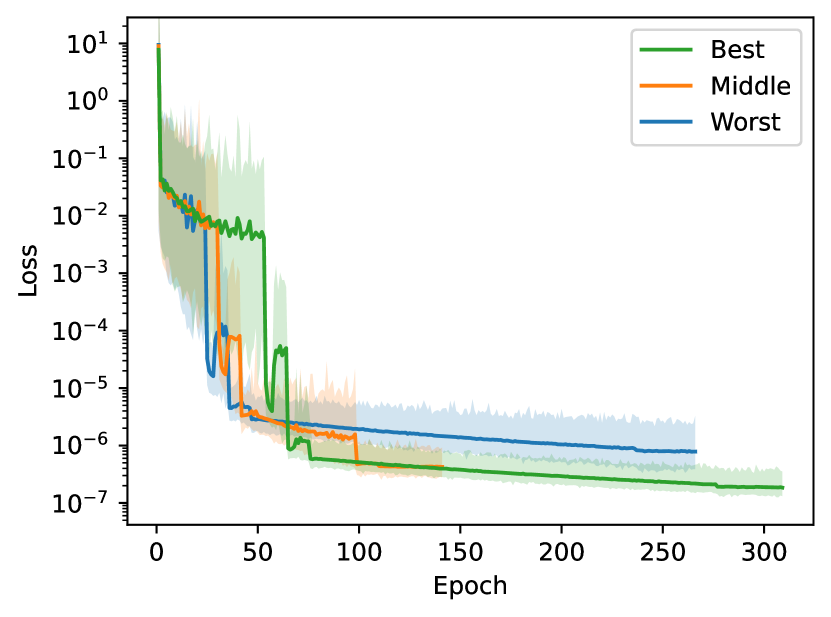
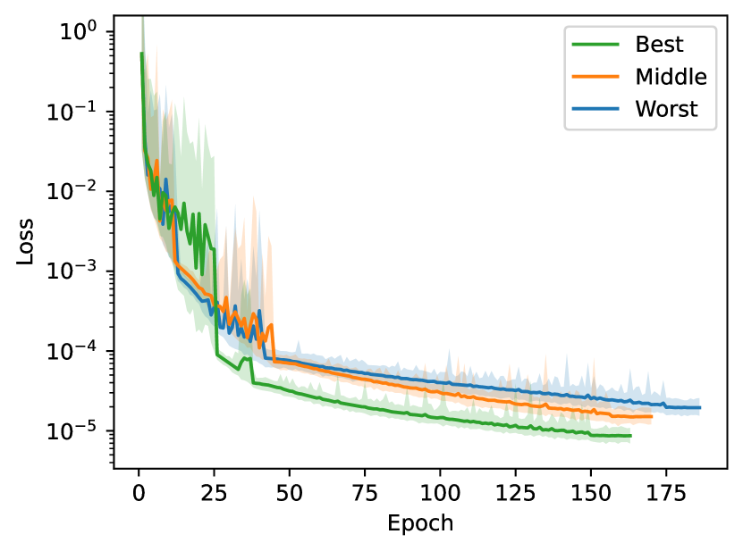
For each example, we show representative learning curves for the training of the replicas of the real parts — being the more difficult component — in the ensemble. Recall that since the training dataset is dynamically generated, the loss function is used for both the training and validation metrics. The loss function is plotted by its mean value per epoch, with bands included to show the maximum and minimum value per epoch. The replica training runs are sorted by the final loss value and, except for section 4.4, three runs are shown: the run with the lowest value, denoted “Best”; the run with the closest to mean value, named “Middle”; and the run with the highest value, as “Worst”. We also include the average training time for a single NN as measured on a laptop.

For examples with two-dimensional inputs, we plot the physical region after applying physical and spurious cuts, together with the points of the boundary dataset.

We perform testing on the trained models and report on the measured errors as defined in section 3.5. We histogram the distributions of the testing errors, binning cumulatively over various subsets of the axes (real or imaginary part, function index, $\epsilon$ order) of the (nonzero) ensemble outputs.

In section 4.5, we discuss a number of features which appear to be common to all examples, and gather a few tables detailing the hyperparameters we used and summarising the comparisons between our models and the testing datasets.

4.1 Massless box

(a) Learning curve.

(b) Absolute difference (real vs. imaginary).

(c) Absolute difference ($\epsilon$ orders).

(d) Magnitude of relative difference ($\epsilon$ orders).

(e) Logarithm of ratio ($\epsilon$ orders).

(f) Errors binned over the phase space.

Figure 3: Training, testing, and inference statistics for the massless box. In figure 3(f), $t$ is the kinematic invariant defined in section 2.1.

We refer to section 2.1 for all definitions of the massless box. We recall that this family has ${n_{F}}=3$ MIs, which depend on ${n_{v}}=2$ kinematic variables, $\vec{v}=\{s,t\}$. Since we do not want to rely on the canonical form of the DEs, we use the MIs defined in eq. 6. We further multiply them by suitable factors of $s$ to cancel their scaling dimensions. The connection matrices are linear in $\epsilon$ (hence $k_{\rm max}=1$). The $\epsilon$ expansion of the MIs in eq. 2 starts from $w^{*}=-2$, and we truncate it at $\epsilon^{2}$, thus considering $n_{\epsilon}=5$ orders ($w_{\rm max}=4$).

We work in the $s$ channel, where $s>-t>0$. Both the physical singularities ($s=0$ and $t=0$) and the spurious singularity ($s+t=0$) are at the boundary of the $s$ channel. No cuts are thus needed to remove the spurious singularities from the DE dataset. The cut on the physical singularities is $10\%$ of $s$, which we fix to $c_{s}=10$. The NNs thus have only one input, $\vec{x}=(c_{s}\,t/s)$, and ${n_{F}}\,{n_{\epsilon}}=15$ outputs. We find that 3 hidden layers of 32 nodes each are sufficient to fit the solution. The relevant values of the hyperparameters are summarised in table 1.

In order to obtain the required boundary values and test our model, we solve the DEs analytically in terms of MPLs (see e.g. eq. 13) in the Euclidean region, and continue the solution to the $s$-channel by adding infinitesimal positive imaginary parts to $s$ and $t$. We evaluate the MPLs using handyG Naterop:2019xaf . The boundary dataset comprises 2 points taken on the edge points of the cut $s$ channel.

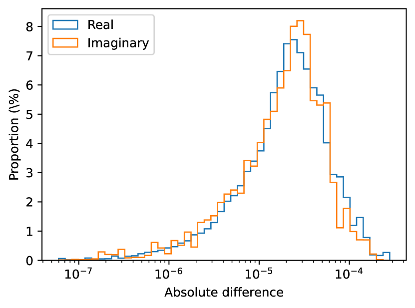
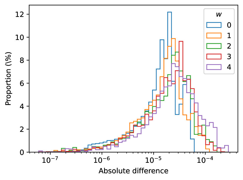
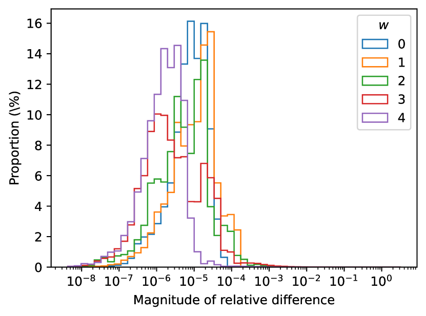
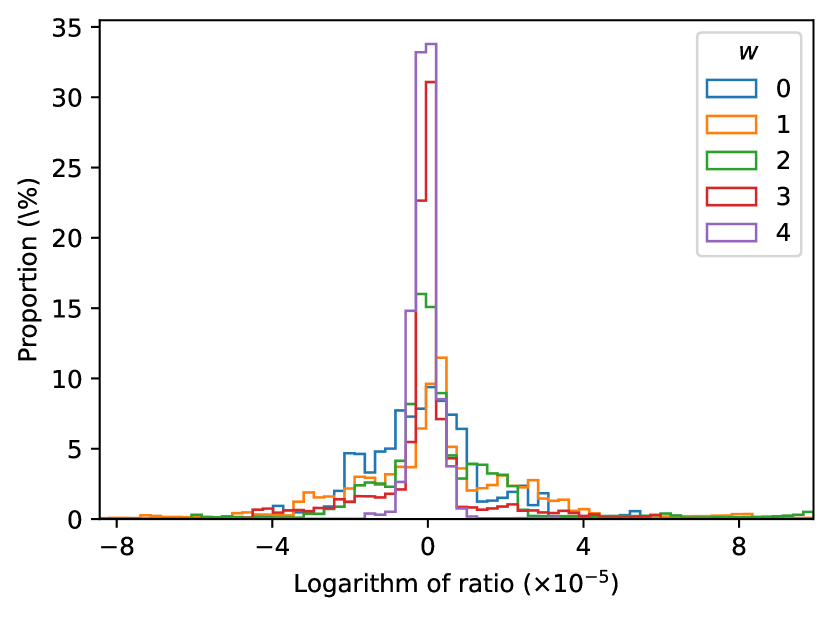
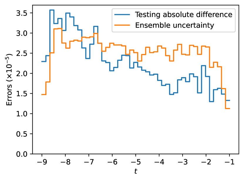
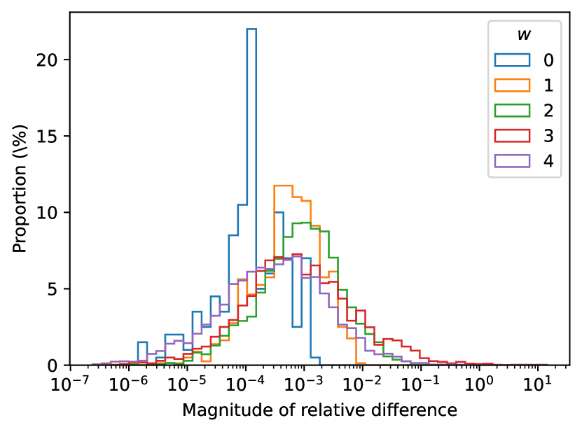
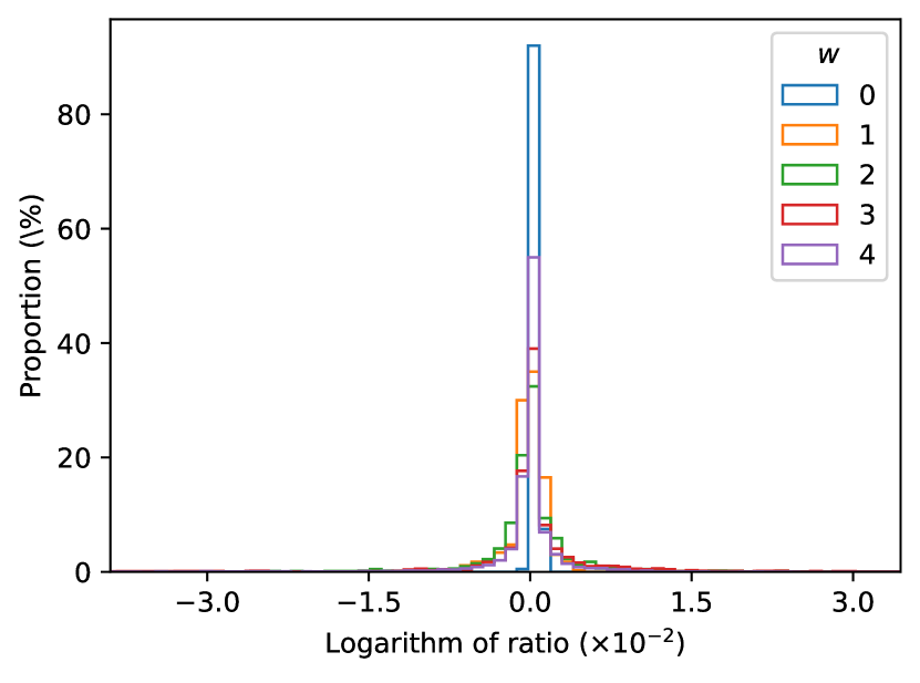
In figure 3(a) we show the learning curve of the ensemble, namely the value of the loss function for the real parts evaluated on the training dataset (see section 3.4). Training of a single NN takes 16 minutes on average. In figures 3(b), 3(c), 3(d) and 3(e) we detail in various ways the comparison between our ensemble and the analytic results on a testing dataset of $10^{5}$ points. Figure 3(b) shows a histogram of the absolute difference, distinguishing real and imaginary parts. Despite the real parts being substantially more complicated, the NNs perform similarly well for them as for the imaginary parts. A similar observation can be made for the different orders in $\epsilon$ of the solution, as seen in figure 3(c). The cumulative mean absolute difference is $2.9\times 10^{-5}$. In figures 3(d) and 3(e) we show the magnitude of the relative difference and the logarithm of the ratio, distinguishing the orders in $\epsilon$. The analytic complexity grows with the order in $\epsilon$, yet the NNs perform comparably well at all orders. The logarithmic ratio histograms are narrow and closely zero-centred, albeit with a small number of outliers. The logarithmic ratio has a cumulative mean value of $3.9\times 10^{-7}$, while the overall mean magnitude of relative difference is $2.2\times 10^{-5}$. Finally, in figure 3(f) we compare the ensemble uncertainty against the testing absolute difference. The ensemble uncertainty proves to be a good estimate of the uncertainty of the fit, as it is compatible with the testing error throughout the phase-space region under consideration.

4.2 Two-loop four-point planar with an external mass

Figure 4: Graph representing the propagator structure of the one-mass double box integral family. The arrows denote the directions of the momenta. Bold lines are massive.

(a) Scattering region with boundary points.

(b) Learning curve.

(c) Magnitude of relative difference ($\epsilon$ orders).

(d) Logarithm of ratio ($\epsilon$ orders).

Figure 5: Training and testing statistics for the one-mass double box.

We now consider the family of Feynman integrals represented by the graph in figure 4. We dub it one-mass double box. These integrals have been computed analytically in refs. Gehrmann:2000zt ; Gehrmann:2002zr ; Duhr:2012fh ; Badger:2023xtl ; Fadin:2023phc . We use the results of ref. Badger:2023xtl to construct the boundary dataset and test the model.

There are ${n_{F}}=18$ MIs, which depend on ${n_{v}}=3$ kinematic variables. We choose $\vec{v}=\{s_{12},s_{23},s_{4}\}$, with $s_{ij}=(p_{i}+p_{j})^{2}$ and $s_{4}=p_{4}^{2}$ ($p_{i}^{2}=0$ for $i=1,2,3$). We use the MI basis of ref. Badger:2023xtl , but remove the normalisation factors which make it canonical. The connection matrices are then linear in $\epsilon$ ($k_{\rm max}=1$). The $\epsilon$ expansion of the MIs in eq. 2 starts from $w^{*}=-4$, and we truncate it at $\epsilon^{0}$, thus considering $n_{\epsilon}=5$ orders ($w_{\rm max}=4$). In this case we do not observe any benefit from cancelling the scaling dimensions of the MIs, and thus refrain from doing so.

We consider the $s_{12}$ channel:

$$s_{12}>s_{4}-s_{23}\,\land\,s_{23}<0\,\land\,s_{4}>0\,.$$ (38)

The physical singularities are at the boundary of this region,

$$s_{12}=0\,,\qquad\quad s_{23}=0\,,\qquad\quad s_{4}=0\,,\qquad\quad s_{12}+s_{23}-s_{4}=0\,.$$ (39)

We impose a cut on them equal to $10\%$ of $s_{12}$, which we fix to $c_{s_{12}}=2.5$. The spurious singularities are

$$s_{12}-s_{4}=0\,,\qquad\quad s_{23}-s_{4}=0\,,\qquad\quad s_{12}+s_{23}=0\,.$$ (40)

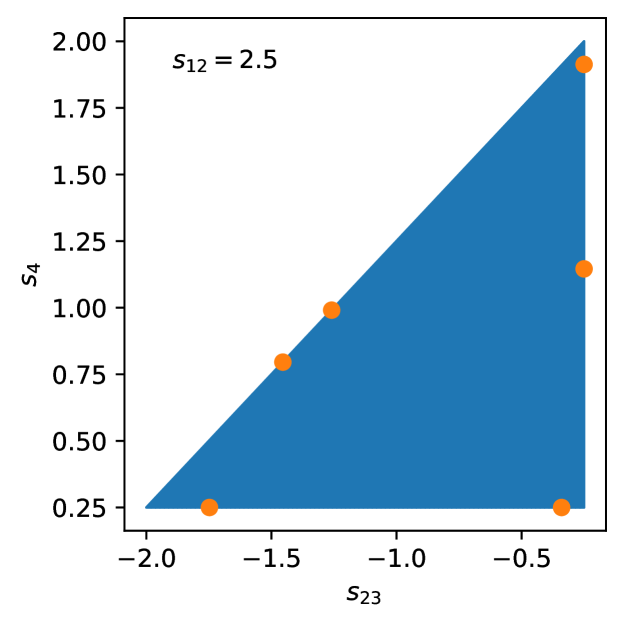
They lie outside of the $s_{12}$ channel and thus do not need to be cut. The boundary dataset comprises 6 points distributed on the boundary of the cut $s_{12}$ channel, as shown in figure 5(a).

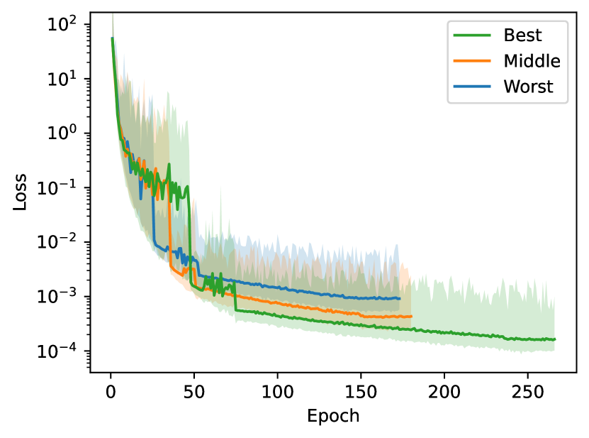
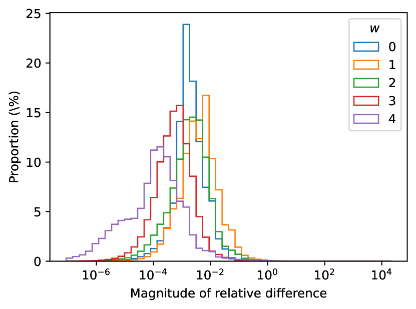
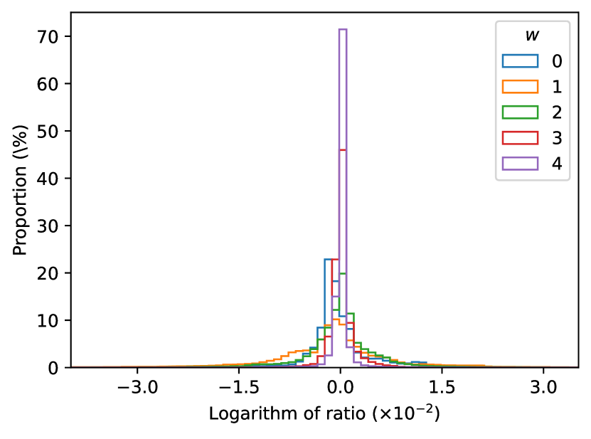
The step-up in difficulty of the one-mass double box is considerable compared to the one-loop massless box. The model input is now two-dimensional, while the output has a 6 times greater size and describes more complicated functions. However, our model still trains well as shown by the learning curve in figure 5(b). Training of a single NN takes around 53 minutes. The observations made for the box in section 4.1 hold true here too: real and imaginary parts, as well as the different orders in $\epsilon$, are learnt by our model equally well. For example, we compare our model against the analytic solutions order by order in $\epsilon$ at $10^{5}$ points in figures 5(c) and 5(d), showing the magnitude of the relative difference and the logarithm of the ratio, respectively. Our model achieves a mean magnitude of relative difference of $1.1\times 10^{-2}$, with a mean logarithm of ratio of $-2.8\times 10^{-4}$.

4.3 Two-loop four-point non-planar with a closed massive loop

Figure 6: Graph representing the propagator structure of the heavy crossed box integral family. The arrows denote the directions of the momenta. Bold lines are massive.

(a) Scattering region with boundary points.

(b) Learning curve.

(c) Magnitude of relative difference ($\epsilon$ orders).

(d) Logarithm of ratio ($\epsilon$ orders).

Figure 7: Training and testing statistics for the heavy crossed box.

In this section, we study the family of non-planar two-loop four-point integrals represented by the graph in figure 6. We dub this family heavy crossed box. With respect to the two-loop four-point integrals discussed in the previous sections, the heavy crossed boxes are non-planar and have a closed loop of massive propagators. The jump in complexity, from the analytic point of view, is substantial. This is in fact the first example we present where the solution cannot be expressed in terms of MPLs. While an analytic expression in terms of elliptic MPLs Broedel:2019hyg has been obtained in ref. vonManteuffel:2017hms for a subsector (i.e., for a subset of integrals where some of the propagator powers are set to zero), the analytic expression of all MIs and a system of DEs in canonical form are still unknown. A full computation was completed only very recently Becchetti:2023wev ; Becchetti:2023yat by solving the DEs numerically with the method of generalised power series expansions Moriello:2019yhu implemented in DiffExp Hidding:2020ytt . To evaluate these integrals numerically in order to create the boundary dataset and test our model we use AMFlow Liu:2017jxz ; Liu:2021wks ; Liu:2022chg with a target precision of 16 digits. While the latter can evaluate these integrals easily, with our method we aim at achieving an evaluation time that is several orders of magnitude shorter.

There are ${n_{F}}=36$ MIs, which depend on ${n_{v}}=3$ kinematic variables. We choose $\vec{v}=\{s,t,m^{2}\}$, with $s=(p_{1}+p_{2})^{2}$ and $t=(p_{1}-p_{3})^{2}$, while $m^{2}$ is the mass of the internal propagators. We use a modification of the MI basis of ref. Becchetti:2023wev . We remove all normalisation factors which contain square roots, so that the connection matrices are rational functions of the kinematics, and multiply the MIs by suitable factors of $m^{2}$ to cancel their scaling dimensions. The connection matrices are polynomial in $\epsilon$ up to order $k_{\rm max}=2$, in contrast with the previous two examples where they were linear. The $\epsilon$ expansion of the MIs in eq. 2 starts from $w^{*}=-4$, and we truncate it at $\epsilon^{0}$, thus considering $n_{\epsilon}=5$ orders ($w_{\rm max}=4$).

We consider the $s_{12}$ channel,

$$s>-t>0\,\land\,m^{2}>0.$$ (41)

We fix $m^{2}$ to $c_{m^{2}}=1$. The physical singularities are where any of the following $4$ factors vanish,

$$\bigl{\{}m^{2}\,,\ s\,,\ t\,,\ s+t\bigr{\}}\,,$$ (42)

while the spurious singularities are associated with the following $9$ factors,

$$\begin{aligned} \bigl{\{}&s-4m^{2}\,,\ s+4m^{2}\,,\ s+16m^{2}\,,\ s+t+4m^{2}\,,\ t-4m^{2}\,,\\ &t-8m^{2}\,,\ s(s+t)-4m^{2}t\,,\ t(s+t)-4m^{2}s\,,\ st-4m^{2}(s+t)\bigr{\}}\,.\end{aligned}$$ (43)

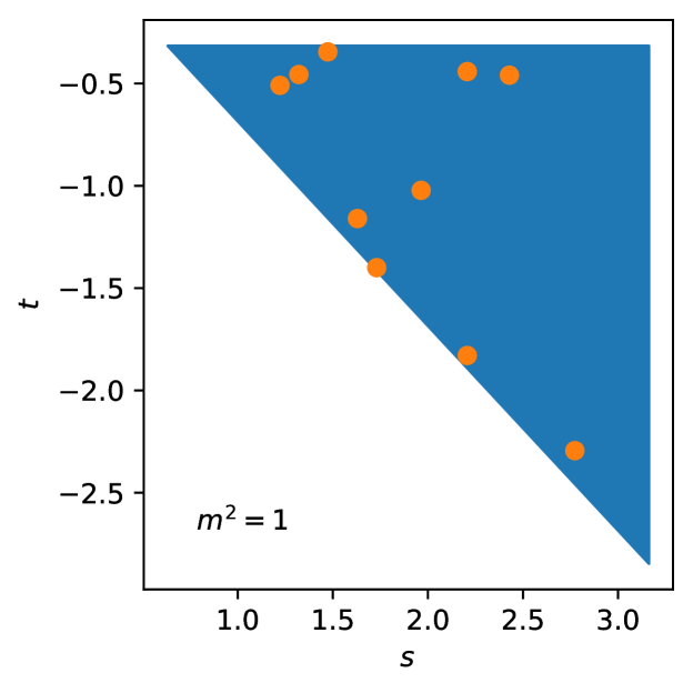
The first spurious singularity, $s=4m^{2}$, crosses the physical region. We prefer to postpone the treatment of spurious singularities to the next example, and focus here on the additional complexity due to the non-polylogarithmic special functions involved in the solution. This allows for a more fair comparison against the results of the previous section. For this reason we restrict the range of $s$ to $s<\sqrt{10}$, this way excluding the spurious singularity from the domain. We take 10 boundary points, randomly sampled from the scattering region as shown in figure 7(a).

As for the previous examples, we plot the decay of the loss function as our learning curve in figure 7(b). This time the training of a single NN takes around 75 minutes. The logarithmic ratio has a cumulative mean of absolute value $4.5\times 10^{-4}$ and the mean magnitude of the relative difference amounts to $7.3\times 10^{-3}$. In figure 7(c) and figure 7(d) we respectively show the magnitude of the relative difference and the logarithm of the ratio, in the various $\epsilon$ orders. Again we note how the performance does not depend on the analytic complexity, which increases with the order in the $\epsilon$ expansion. The fact that the order $\epsilon^{0}$ appears to perform better than the higher orders in figure 7(c) is misleading. One should in fact note that, conversely, the order $\epsilon^{4}$ is doing better than the simpler order $\epsilon^{3}$. In general, the performance of the model for the single MI coefficient is uncorrelated to its analytic complexity.

4.4 Two-loop four-point planar for top-pair production with a closed top loop

Figure 8: Graph representing the propagator structure of the top double box integral family. The arrows denote the directions of the momenta. Bold lines are massive.

(a) Scattering region with boundary points.

(b) Learning curve.

(c) Magnitude of relative difference ($\epsilon$ orders).

(d) Logarithm of ratio ($\epsilon$ orders).

Figure 9: Training and testing statistics for the top double box.

Our final and most complicated example is the family of integrals associated with the graph in figure 8, which we dub top double box. The top double box integrals were first computed by solving numerically the DEs Czakon:2013goa ; Barnreuther:2013qvf . The analytic study of refs. Adams:2018kez ; Adams:2018bsn later revealed an extreme degree of analytic complexity. The presence of three inequivalent elliptic curves puts this integral family at the cutting edge of analytic computations. Indeed, a canonical form of the DEs has become available recently only for a subsector Muller:2022gec . In refs. Adams:2018kez ; Adams:2018bsn , instead, the authors obtained connection matrices linear in $\epsilon$, and with a block triangular structure which allows for a solution in terms of Chen iterated integrals Chen:1977oja . Nonetheless, the numerical evaluation of these functions remains challenging (see e.g. Badger:2021owl ). As in the previous example, therefore, we rely on AMFlow for evaluating the MIs numerically, using a target precision of 10 digits.

There are $44$ MIs, which depend on ${n_{v}}=3$ kinematic variables. We choose $\vec{v}=\{s_{12},s_{23},m_{\rm t}^{2}\}$, with $s_{ij}=(p_{i}+p_{j})^{2}$ and $p_{3}^{2}=p_{4}^{2}=m_{\rm t}^{2}$ ($p_{1}^{2}=p_{2}^{2}=0$). We constructed a MI basis such that the dependence on $\epsilon$ is factorised from the dependence on the kinematics in the denominators of the connection matrices Smirnov:2020quc ; Usovitsch:2020jrk , and normalised some of the MIs by factors of $\epsilon$ to make the connection matrices finite at $\epsilon=0$. The resulting connection matrices are rational functions of $\epsilon$. We Taylor expand them around $\epsilon=0$. Note that the internal mass regulates the infrared divergences. As a result, the $\epsilon$ expansion of the MIs in eq. 2 starts from $w^{*}=-2$ rather than $-4$ as in the other two-loop examples. By truncating the expansion at $\epsilon^{0}$ we then consider $n_{\epsilon}=3$ orders ($w_{\rm max}=2$). For this we only need the connection matrices up to $\epsilon^{2}$. The higher orders are neglected. From the boundary dataset we can also determine that, up to $\epsilon^{0}$, $11$ of the $44$ MIs vanish identically. We thus eliminate them from the system, leaving ${n_{F}}=33$ nonzero MIs.

We consider the $s_{12}$ channel,

$$s_{12}>4m_{\rm t}^{2}>0\,\land\,s_{23}(s_{12}+s_{23})-2m_{\rm t}^{2}s_{23}+m_{\rm t}^{4}<0\,.$$ (44)

We fix $m_{\rm t}^{2}$ to $c_{m_{\text{t}}^{2}}=1$, and vary $s_{12}$ in $(0,5)$. The physical singularities are associated with the following $4$ factors,

$$\bigl{\{}m_{\rm t}^{2}\,,\ s_{12}\,,\ s_{23}\,,\ s_{23}(s_{12}+s_{23})-2m_{\rm t}^{2}s_{23}+m_{\rm t}^{4}\bigr{\}}\,,$$ (45)

and there is a spurious singularity where any of the following $8$ factors vanish,

$$\begin{aligned} \bigl{\{}&m_{\rm t}^{2}+s_{23}\,,\ s_{12}+4m_{\rm t}^{2}\,,\ s_{23}-m_{\rm t}^{2}\,,\ s_{12}-4m_{\rm t}^{2}\,,\ s_{23}-9m_{\rm t}^{2}\,,\ s_{12}+s_{23}-m_{\rm t}^{2}\,,\\ &s_{12}s_{23}-9m_{\rm t}^{2}s_{12}-4m_{\rm t}^{2}s_{23}+4m_{\rm t}^{4}\,,\ 64m_{\rm t}^{6}-9m_{\rm t}^{4}s_{12}+10m_{\rm t}^{2}s_{12}s_{23}-s_{12}s_{23}^{2}\bigr{\}}\,.\end{aligned}$$ (46)

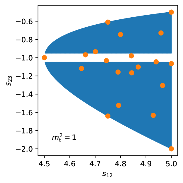
The first spurious singularity, $s_{23}+m_{\rm t}^{2}=0$, crosses the $s_{12}$ channel. Therefore, in addition to the cut on the physical singularities at the boundary of the $s_{12}$ channel, we also need a cut to exclude the spurious singularity from the DE dataset. We choose $10\%$ of the largest value of $s_{12}$ for the former, and $1\%$ for the latter. The shape of the $s_{12}$ channel and the spurious cut crossing it are shown in figure 9(a). We stress that this is a novel feature, absent in the previous examples. We take 20 boundary points, with 5 manually placed on the boundaries and the remaining 15 randomly sampled from the interior of the physical region.

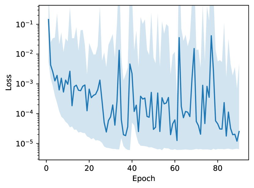
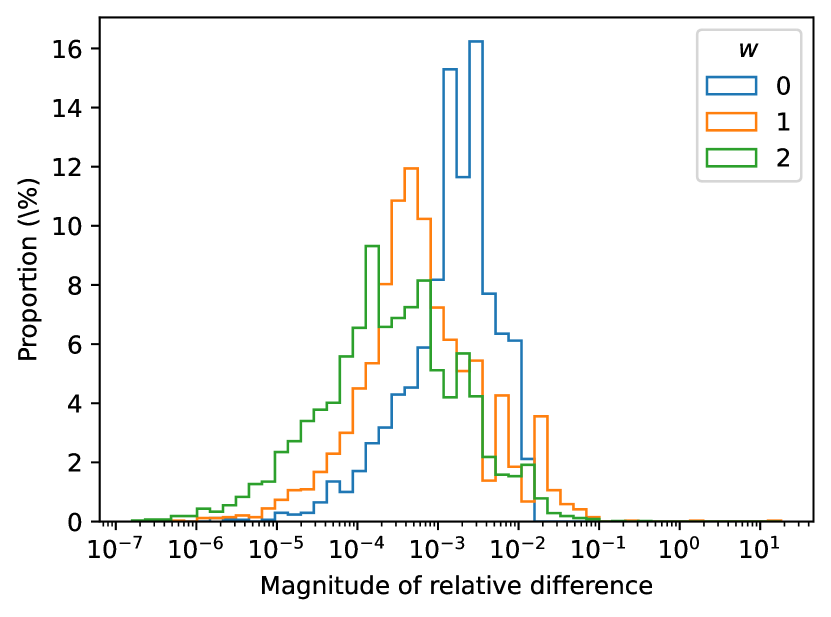
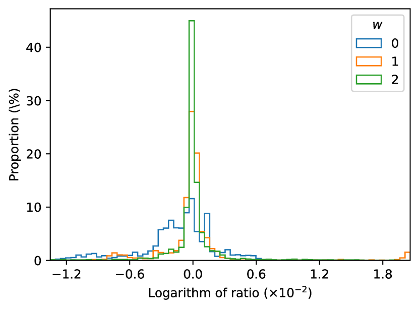
While for the previous examples we found that three hidden layers were sufficient, we see a performance improvement by moving to four layers for the top double box. We plot the learning curve in figure 9(b), where the difficulty in training at this level of analytic complexity is revealed by the instability of the loss function. Indeed, in order to make the figure clearer, in this case we plot only the “best” learning curve, namely the one ending with the lowest loss value. We observe that this is a result of a small fraction of training points being pathological, which was not regulated by increasing the cuts. This time the training of a single NN takes around 32 minutes. In testing, the performance of the basis functions varied by up to an order of magnitude as measured by the mean absolute difference per basis function. However, the average fit is good, with a cumulative mean of the logarithmic ratio of $1.4\times 10^{-3}$ and a mean magnitude of the relative difference of $3.9\times 10^{-3}$. Figures 9(c) and 9(d) respectively show the distributions of the magnitude of the relative difference and the logarithm of the ratio, in the successive $\epsilon$ orders. For this example, we found some replica trainings to fail, having a differential error in validation up to a few times larger than the others. We discarded these replicas and re-trained replacements.

4.5 General comments

Before discussing the general features we observed in the previous examples, we collect here a number of common tables to facilitate the comparison. In table 1 we summarise the hyperparameters we used, table 2 gives some statistics on the training, and table 3 describes the comparison between our models and the testing dataset. We emphasise that the last two examples (the heavy crossed box and the top double box) have lower statistics than the first two (the massless box and the one-mass double box), because we had to rely on AMFlow for the numerical evaluation of the integrals in the former, as opposed to the analytic results available for the latter.

Integral family	box	one-mass double box	heavy crossed box	top double box
Inputs	1	2	2	2
Hidden layers	$3\times 32$	$3\times 256$	$3\times 256$	$4\times 128$
Outputs	15	90	180	99
Learning rate	$10^{-2}$	$10^{-3}$	$10^{-3}$	$10^{-3}$
Batch size	64	256	256	256
Boundary points	2	6	10	20
$c_{{n_{v}}}$	$s=10$	$s_{12}=2.5$	$m^{2}=1$	$m_{\text{t}}^{2}=1$
Scale bound	—	—	$s\leq\sqrt{10}$	$s_{12}\leq 5$
Physical cut (%)	10	10	10	10
Spurious cut (%)	0	0	0	1

Table 1: Summary of hyperparameters for all examples, showing NN architecture (inputs, hidden layers depth $\times$ width, outputs), initial learning rate, training batch size, number of boundary points, value and index of kinematic constant $c_{{n_{v}}}$, kinematic scale bound (if applicable), physical cut size, and spurious cut size. The same hyperparameters are used to train NNs for both the real and imaginary parts of the solutions.

Integral family	Final loss	Iterations	Time (minutes)
box	$2.7\times 10^{-7}$	$2.5\times 10^{5}$	16
one-mass double box	$3.4\times 10^{-4}$	$1.1\times 10^{5}$	53
heavy crossed box	$1.4\times 10^{-5}$	$7.9\times 10^{4}$	75
top double box	$7.1\times 10^{-4}$	$5.2\times 10^{4}$	32

Table 2: Summary of training statistics for all examples, showing mean loss value of final epoch, mean total number of iterations, and typical time to train a single NN. These results are averaged over all replicas within the ensemble.

Integral family	MEU	MDE	MAD	MMRD	MLR	Size
box	$2.8\times 10^{-5}$	$3.6\times 10^{-4}$	$2.9\times 10^{-5}$	$2.2\times 10^{-5}$	$3.9\times 10^{-7}$	$10^{5}$
one-mass DB	$8.1\times 10^{-4}$	$1.1\times 10^{-2}$	$2.0\times 10^{-3}$	$1.1\times 10^{-2}$	$-2.8\times 10^{-4}$	$10^{5}$
heavy CB	$2.8\times 10^{-4}$	$2.8\times 10^{-3}$	$1.6\times 10^{-3}$	$7.3\times 10^{-3}$	$-4.5\times 10^{-4}$	$10^{2}$
top DB	$1.9\times 10^{-4}$	$1.7\times 10^{-3}$	$9.0\times 10^{-4}$	$3.9\times 10^{-3}$	$1.8\times 10^{-4}$	$10^{2}$

Table 3: Summary of ensemble uncertainty and testing errors as defined in section 3.5 for all examples. We use the shorthands DB and CB for double box and crossed box, respectively. We show mean ensemble uncertainty (MEU), mean differential error (MDE), mean absolute difference (MAD), mean magnitude of relative difference (MMRD), mean logarithm of ratio (MLR), and size of testing dataset. All means are taken over all nonzero outputs of the ensemble, with the exception of the MDE, which is over all nonzero outputs of all replicas.

The first general feature we observe is related to the flatness of the performance of our NNs with respect to the analytic complexity of the learnt functions. From the analytic point of view, the real part of the integrals is more complicated than the imaginary part, the complexity grows with the depth in the $\epsilon$ expansion, and certain MIs are more complicated than others. Our models instead appear to perform equally well for both complex parts, all orders in $\epsilon$, and all MIs of each family.

Similarly, the performance appears to be flat also with respect to the complexity of the example. In other words, after limited hyperparameter tuning, our models reach a similar level of performance for all the two-loop examples we considered. We achieve a mean magnitude of relative difference of roughly 1% for all the two-loop examples considered (see table 3), with training times of the order of one hour on a laptop GPU (see table 2). This is particularly promising, as it indicates that this approach is insensitive to the analytic complexity of the special functions appearing in the solution to the DEs. We recall in fact that, while for the one-mass double box integrals a convenient representation in terms of MPLs is well known, we have a representation in terms of Chen iterated integrals for the top double box integrals (which is not suitable for a fast numerical evaluation in the physical scattering region), and no analytic expression at all for the heavy crossed box. It is important to emphasise however that the two-loop integral families we considered all have the same number of input variables ($2$, after one kinematical variable is fixed to a constant). This warrants the analysis of Feynman integrals depending on more variables, which we defer to future studies.

Another promising observation which calls for a more in-depth study concerns the spurious singularities. As discussed in section 3.2, we impose cuts on the DE dataset around the spurious singularities. These cut regions are instead retained in the boundary and in the testing datasets. In the examples we studied, this is relevant only for the top double box, as in the other cases the spurious singularities fall outside the physical scattering region under consideration. Nonetheless, it is interesting that the extra cut on the DE dataset does not appear to impact the performance of the model for the top double box even in proximity of the spurious singularity. Feynman integrals with more intricate spurious singularities within the physical scattering region of interest should be analysed in the future to confirm this promising observation.

Finally, any numerical value is of little use without a reliable estimate of its uncertainty. In particular, we need a prescription to associate the prediction of our model with an uncertainty without relying on the comparison with a large testing dataset. In this work, we consider two quantities which may give such an estimate: the mean ensemble uncertainty and the mean differential error (see section 3.5). Both of them are absolute measures, and we find them to be correlated to the mean absolute difference in the testing dataset. Associating a reliable uncertainty to the model predictions would however require a more thorough analysis of the correlation between the ensemble uncertainty/differential error and the testing errors, which we leave for future study.

5 Conclusion and outlook

In this paper, we propose a new approach to evaluate Feynman integrals numerically. We view the Feynman integrals as the solutions to systems of first-order PDEs. We compute the PDEs analytically, and train a deep NN to approximate their solution using the recently-proposed framework of physics-informed deep learning (PIDL). The NN takes the kinematic variables as inputs, and returns the values of the integrals expanded around $\epsilon=0$ up to a chosen order, split into real and imaginary parts. The method relies on the analytic expression of the DEs, and on the values of the Feynman integrals at a small number of reference points. Mild assumptions are made on the form of the DEs, merely to simplify the problem, but we do not rely on a canonical form of the DEs. Indeed, our method is aimed in particular at those cases where canonical DEs have not been obtained, or where their analytical solutions contain classes of special functions for which the mathematical technology is not yet fully developed.

We provide a proof-of-concept implementation within the PyTorch framework, and apply it to a number of one- and two-loop integral families. One family is at the cutting edge of current analytical methods, and another is not yet known analytically. In all two-loop examples, we achieve a mean magnitude of relative difference of order 1% in the physical phase space with NN training times on the order of an hour on a laptop GPU. The performance appears to be flat with respect to the analytic complexity of the solutions. In other words, after limited hyperparameter tuning, our models reach a similar level of performance for all examples we considered and, within a single family, for all integrals and all orders in their $\epsilon$ expansion.

With respect to traditional numerical DE solver, semi-analytical DE solvers based on generalised power series expansions, and Monte Carlo integration methods, our approach yields essentially instantaneous evaluation times. The overall time budget is concentrated in the training of the NNs, which however is done once and for all for a given integral family. This however comes at the price of a lower control over the uncertainty. We proposed a number of proxies to estimate the latter, based on the standard error of an ensemble of NNs fitting the solution to the same DEs, and on how well the model satisfies the DEs. However, controlling the accuracy, namely constructing and training a NN such that it reaches a given target accuracy, remains an open problem. This is particularly important for using the integrals in the computation of scattering amplitudes, where large cancellations among different terms may lead to a loss of accuracy.

The question of how to improve the fitting performance of PIDL models is a well-known open challenge hao2023physicsinformed , although a number of refinements are being explored in the literature wang2023experts . Our target functions exhibit features of varied frequencies over a large distribution of scales, which can degrade stochastic gradient descent by introducing unbalanced back-propagated gradients wang2020understanding ; wang2020pinns , while NNs are biased towards learning global fluctuations over local details pmlr-v97-rahaman19a ; ijcai2021p304 . Of particular promise for our application are attempts to balance the training algorithm in order to address these issues, such as adaptive sampling of the phase space Nabian_2021 ; daw2023mitigating ; Wu_2023 or adaptive reweighting of the loss function wang2020understanding ; wang2020pinns ; MCCLENNY2023111722 ; Maddu_2022 .

In addition to these developments on the machine learning side, there is room for improvement also on the physics side. Even when the integrals cannot be computed analytically, a lot is known about their asymptotic behaviour in the singular limits, either from the DEs themselves or through other approaches such as the method of regions Beneke:1997zp ; Smirnov:1999bza ; Jantzen:2011nz . This precious information may be used for instance to partition the phase space based on the infrared singularities and then train a different NN in each sub-region Badger:2020uow ; Aylett-Bullock:2021hmo . Furthermore, one could impose hard constraints in the form of an ansatz with NNs as coefficients, along the lines of the factorisation-aware matrix-element emulation proposed in refs. Maitre:2021uaa ; Janssen:2023ahv ; Maitre:2023dqz .

Given the successful proof of concept discussed in this paper and the large room for improvement, we believe that this novel method has the potential to increase the evaluation efficiency of Feynman integrals for which the analytic solution is still out of reach.

Appendix A Integral family definitions

In this appendix, we collect the definitions of the propagators of the two-loop four-point integral families studied in section 4. They all have 7 propagators, followed by 2 auxiliary propagators (called as irreducible scalar products), which are required in order to accommodate into the integral family any numerator over the given propagator structure. The integrals of each family have the form

$$\mathrm{I}_{\vec{a}}(\vec{v};\epsilon)=\int\frac{\text{d}^{d}k_{1}}{\mathrm{i}\pi^{d/2}}\frac{\text{d}^{d}k_{2}}{\mathrm{i}\pi^{d/2}}\frac{\mu^{2(4-d)}}{D_{1}^{a_{1}}D_{2}^{a_{2}}\cdots D_{9}^{a_{9}}}\,,$$ (47)

where $\vec{v}$ are the independent kinematic variables, $\mu$ is the dimensional regularisation scale, $\vec{a}=(a_{1},\ldots,a_{9})\in\mathbb{Z}^{9}$, and $D_{i}$ are the inverse propagators. The last two are ISPs, hence $a_{8},a_{9}\leq 0$. We set $\mu=1$. We define below the inverse propagators $D_{i}$ family by family, omitting Feynman’s $\mathrm{i}0^{+}$ prescription.

One-mass double box (figure 4)

$$\begin{aligned} \{D_{i}\}_{i=1}^{9}=\bigl{\{}&k_{1}^{2},\,(k_{1}-p_{1})^{2},\,(k_{1}-p_{1}-p_{2})^{2},\,k_{2}^{2},\,(k_{2}-p_{4})^{2},\,\\ &(k_{2}+p_{1}+p_{2})^{2},\,(k_{1}+k_{2})^{2},\,(k_{1}+p_{4})^{2},\,(k_{2}+p_{1})^{2}\bigr{\}}\,.\end{aligned}$$ (48)

Heavy crossed box (figure 6)

$$\begin{aligned} \{D_{i}\}_{i=1}^{9}=\bigl{\{}&k_{1}^{2},\,(k_{1}-p_{1})^{2},\,(k_{1}+p_{2})^{2},\,k_{2}^{2}-m^{2},\,(k_{1}+k_{2}-p_{1})^{2}-m^{2},\\ &(k_{2}-p_{4})^{2}-m^{2},\,(k_{1}+k_{2}-p_{1}+p_{3})^{2}-m^{2},\,(k_{1}+p_{3})^{2},\,(k_{1}+k_{2})^{2}\}\,.\end{aligned}$$ (49)

Top double box (figure 8)

$$\begin{aligned} \{D_{i}\}_{i=1}^{9}=\bigl{\{}&k_{1}^{2}-m_{\rm t}^{2},\,(k_{1}-p_{1})^{2}-m_{\rm t}^{2},\,(k_{1}-p_{1}-p_{2})^{2}-m_{\rm t}^{2},\,k_{2}^{2},\,(k_{2}-p_{4})^{2}-m_{\rm t}^{2}\\ &(k_{2}-p_{3}-p_{4})^{2},\,(k_{1}+k_{2})^{2}-m_{\rm t}^{2},\,(k_{1}+p_{4})^{2},\,(k_{2}+p_{1})^{2}\bigr{\}}\,.\end{aligned}$$ (50)

References

- (1) G. Barucchi and G. Ponzano, Differential equations for one-loop generalized Feynman integrals, J. Math. Phys. 14 (1973) 396.
- (2) A.V. Kotikov, Differential equations method: New technique for massive Feynman diagrams calculation, Phys. Lett. B 254 (1991) 158.
- (3) A.V. Kotikov, Differential equations method: The Calculation of vertex type Feynman diagrams, Phys. Lett. B 259 (1991) 314.
- (4) T. Gehrmann and E. Remiddi, Differential equations for two loop four point functions, Nucl. Phys. B 580 (2000) 485 [hep-ph/9912329].
- (5) Z. Bern, L.J. Dixon and D.A. Kosower, Dimensionally regulated pentagon integrals, Nucl. Phys. B 412 (1994) 751 [hep-ph/9306240].
- (6) J.M. Henn, Multiloop integrals in dimensional regularization made simple, Phys. Rev. Lett. 110 (2013) 251601 [1304.1806].
- (7) S. Pozzorini and E. Remiddi, Precise numerical evaluation of the two loop sunrise graph master integrals in the equal mass case, Comput. Phys. Commun. 175 (2006) 381 [hep-ph/0505041].
- (8) U. Aglietti, R. Bonciani, L. Grassi and E. Remiddi, The Two loop crossed ladder vertex diagram with two massive exchanges, Nucl. Phys. B 789 (2008) 45 [0705.2616].
- (9) R.N. Lee, A.V. Smirnov and V.A. Smirnov, Solving differential equations for Feynman integrals by expansions near singular points, JHEP 03 (2018) 008 [1709.07525].
- (10) R.N. Lee, A.V. Smirnov and V.A. Smirnov, Evaluating ‘elliptic’ master integrals at special kinematic values: using differential equations and their solutions via expansions near singular points, JHEP 07 (2018) 102 [1805.00227].
- (11) R. Bonciani, G. Degrassi, P.P. Giardino and R. Gröber, A Numerical Routine for the Crossed Vertex Diagram with a Massive-Particle Loop, Comput. Phys. Commun. 241 (2019) 122 [1812.02698].
- (12) M. Fael, F. Lange, K. Schönwald and M. Steinhauser, A semi-analytic method to compute Feynman integrals applied to four-loop corrections to the -pole quark mass relation, JHEP 09 (2021) 152 [2106.05296].
- (13) M. Fael, F. Lange, K. Schönwald and M. Steinhauser, Massive Vector Form Factors to Three Loops, Phys. Rev. Lett. 128 (2022) 172003 [2202.05276].
- (14) X. Liu, Y.-Q. Ma and C.-Y. Wang, A Systematic and Efficient Method to Compute Multi-loop Master Integrals, Phys. Lett. B 779 (2018) 353 [1711.09572].
- (15) F. Moriello, Generalised power series expansions for the elliptic planar families of Higgs + jet production at two loops, JHEP 01 (2020) 150 [1907.13234].
- (16) M. Hidding, DiffExp, a Mathematica package for computing Feynman integrals in terms of one-dimensional series expansions, Comput. Phys. Commun. 269 (2021) 108125 [2006.05510].
- (17) X. Liu and Y.-Q. Ma, Multiloop corrections for collider processes using auxiliary mass flow, Phys. Rev. D 105 (2022) L051503 [2107.01864].
- (18) X. Liu and Y.-Q. Ma, AMFlow: A Mathematica package for Feynman integrals computation via auxiliary mass flow, Comput. Phys. Commun. 283 (2023) 108565 [2201.11669].
- (19) T. Armadillo, R. Bonciani, S. Devoto, N. Rana and A. Vicini, Evaluation of Feynman integrals with arbitrary complex masses via series expansions, Comput. Phys. Commun. 282 (2023) 108545 [2205.03345].
- (20) T. Binoth and G. Heinrich, An automatized algorithm to compute infrared divergent multiloop integrals, Nucl. Phys. B 585 (2000) 741 [hep-ph/0004013].
- (21) C. Bogner and S. Weinzierl, Resolution of singularities for multi-loop integrals, Comput. Phys. Commun. 178 (2008) 596 [0709.4092].
- (22) T. Kaneko and T. Ueda, A Geometric method of sector decomposition, Comput. Phys. Commun. 181 (2010) 1352 [0908.2897].
- (23) S. Borowka, J. Carter and G. Heinrich, Numerical Evaluation of Multi-Loop Integrals for Arbitrary Kinematics with SecDec 2.0, Comput. Phys. Commun. 184 (2013) 396 [1204.4152].
- (24) S. Borowka, G. Heinrich, S.P. Jones, M. Kerner, J. Schlenk and T. Zirke, SecDec-3.0: numerical evaluation of multi-scale integrals beyond one loop, Comput. Phys. Commun. 196 (2015) 470 [1502.06595].
- (25) S. Borowka, G. Heinrich, S. Jahn, S.P. Jones, M. Kerner, J. Schlenk et al., pySecDec: a toolbox for the numerical evaluation of multi-scale integrals, Comput. Phys. Commun. 222 (2018) 313 [1703.09692].
- (26) S. Borowka, G. Heinrich, S. Jahn, S.P. Jones, M. Kerner and J. Schlenk, A GPU compatible quasi-Monte Carlo integrator interfaced to pySecDec, Comput. Phys. Commun. 240 (2019) 120 [1811.11720].
- (27) G. Heinrich, S.P. Jones, M. Kerner, V. Magerya, A. Olsson and J. Schlenk, Numerical Scattering Amplitudes with pySecDec, 2305.19768.
- (28) A.V. Smirnov and M.N. Tentyukov, Feynman Integral Evaluation by a Sector decomposiTion Approach (FIESTA), Comput. Phys. Commun. 180 (2009) 735 [0807.4129].
- (29) A.V. Smirnov, V.A. Smirnov and M. Tentyukov, FIESTA 2: Parallelizeable multiloop numerical calculations, Comput. Phys. Commun. 182 (2011) 790 [0912.0158].
- (30) A.V. Smirnov, FIESTA 3: cluster-parallelizable multiloop numerical calculations in physical regions, Comput. Phys. Commun. 185 (2014) 2090 [1312.3186].
- (31) A.V. Smirnov, FIESTA4: Optimized Feynman integral calculations with GPU support, Comput. Phys. Commun. 204 (2016) 189 [1511.03614].
- (32) A.V. Smirnov, N.D. Shapurov and L.I. Vysotsky, FIESTA5: Numerical high-performance Feynman integral evaluation, Comput. Phys. Commun. 277 (2022) 108386 [2110.11660].
- (33) N.I. Usyukina and A.I. Davydychev, An Approach to the evaluation of three and four point ladder diagrams, Phys. Lett. B 298 (1993) 363.
- (34) N.I. Usyukina and A.I. Davydychev, Exact results for three and four point ladder diagrams with an arbitrary number of rungs, Phys. Lett. B 305 (1993) 136.
- (35) V.A. Smirnov, Analytical result for dimensionally regularized massless on shell double box, Phys. Lett. B 460 (1999) 397 [hep-ph/9905323].
- (36) J.B. Tausk, Nonplanar massless two loop Feynman diagrams with four on-shell legs, Phys. Lett. B 469 (1999) 225 [hep-ph/9909506].
- (37) M. Czakon, Automatized analytic continuation of Mellin-Barnes integrals, Comput. Phys. Commun. 175 (2006) 559 [hep-ph/0511200].
- (38) A.V. Smirnov and V.A. Smirnov, On the Resolution of Singularities of Multiple Mellin-Barnes Integrals, Eur. Phys. J. C 62 (2009) 445 [0901.0386].
- (39) J. Gluza, K. Kajda and T. Riemann, AMBRE: A Mathematica package for the construction of Mellin-Barnes representations for Feynman integrals, Comput. Phys. Commun. 177 (2007) 879 [0704.2423].
- (40) A.V. Belitsky, A.V. Smirnov and V.A. Smirnov, MB tools reloaded, Nucl. Phys. B 986 (2023) 116067 [2211.00009].
- (41) O.V. Tarasov, Connection between Feynman integrals having different values of the space-time dimension, Phys. Rev. D 54 (1996) 6479 [hep-th/9606018].
- (42) R.N. Lee, Space-time dimensionality D as complex variable: Calculating loop integrals using dimensional recurrence relation and analytical properties with respect to D, Nucl. Phys. B 830 (2010) 474 [0911.0252].
- (43) R.N. Lee and V.A. Smirnov, The Dimensional Recurrence and Analyticity Method for Multicomponent Master Integrals: Using Unitarity Cuts to Construct Homogeneous Solutions, JHEP 12 (2012) 104 [1209.0339].
- (44) F. Brown, The Massless higher-loop two-point function, Commun. Math. Phys. 287 (2009) 925 [0804.1660].
- (45) E. Panzer, Algorithms for the symbolic integration of hyperlogarithms with applications to Feynman integrals, Comput. Phys. Commun. 188 (2015) 148 [1403.3385].
- (46) S. Catani, T. Gleisberg, F. Krauss, G. Rodrigo and J.-C. Winter, From loops to trees by-passing Feynman’s theorem, JHEP 09 (2008) 065 [0804.3170].
- (47) R. Runkel, Z. Szőr, J.P. Vesga and S. Weinzierl, Causality and loop-tree duality at higher loops, Phys. Rev. Lett. 122 (2019) 111603 [1902.02135].
- (48) Z. Capatti, V. Hirschi, D. Kermanschah and B. Ruijl, Loop-Tree Duality for Multiloop Numerical Integration, Phys. Rev. Lett. 123 (2019) 151602 [1906.06138].
- (49) M. Borinsky, Tropical Monte Carlo quadrature for Feynman integrals, 2008.12310.
- (50) M. Borinsky, H.J. Munch and F. Tellander, Tropical Feynman integration in the Minkowski regime, Comput. Phys. Commun. 292 (2023) 108874 [2302.08955].
- (51) M. Zeng, Feynman integrals from positivity constraints, JHEP 09 (2023) 042 [2303.15624].
- (52) V.A. Smirnov, Analytic tools for Feynman integrals, vol. 250 (2012), 10.1007/978-3-642-34886-0.
- (53) S. Weinzierl, Feynman Integrals (1, 2022), 10.1007/978-3-030-99558-4, [2201.03593].
- (54) R. Winterhalder, V. Magerya, E. Villa, S.P. Jones, M. Kerner, A. Butter et al., Targeting multi-loop integrals with neural networks, SciPost Phys. 12 (2022) 129 [2112.09145].
- (55) D. Ma$̂\mathrm{i}$tre and R. Santos-Mateos, Multi-variable integration with a neural network, JHEP 03 (2023) 221 [2211.02834].
- (56) J.M. Cruz-Martinez, M. Robbiati and S. Carrazza, Multi-variable integration with a variational quantum circuit, 2308.05657.
- (57) M. Feickert and B. Nachman, A Living Review of Machine Learning for Particle Physics, 2102.02770.
- (58) S. Badger et al., Machine learning and LHC event generation, SciPost Phys. 14 (2023) 079 [2203.07460].
- (59) HEP ML Community, “A Living Review of Machine Learning for Particle Physics.” https://iml-wg.github.io/HEPML-LivingReview/.
- (60) K. Hornik, M. Stinchcombe and H. White, Multilayer feedforward networks are universal approximators, Neural Networks 2 (1989) 359.
- (61) M. Raissi, P. Perdikaris and G.E. Karniadakis, Physics Informed Deep Learning (Part I): Data-driven Solutions of Nonlinear Partial Differential Equations, 1711.10561.
- (62) M. Raissi, P. Perdikaris and G.E. Karniadakis, Physics Informed Deep Learning (Part II): Data-driven Discovery of Nonlinear Partial Differential Equations, 1711.10566.
- (63) M. Raissi, P. Perdikaris and G.E. Karniadakis, Physics-informed neural networks: A deep learning framework for solving forward and inverse problems involving nonlinear partial differential equations, Journal of Computational Physics 378 (2019) 686.
- (64) A. Dersy, M.D. Schwartz and A. Zhiboedov, Reconstructing -matrix Phases with Machine Learning, 2308.09451.
- (65) F. Calisto, A study of the differential equations method for Feynman loop integrals in connection with Scientific Machine Learning, bachelor’s thesis, University of Torino, 2022.
- (66) R. Moodie, F. Calisto and S. Zoia, “Feynman integral neural networks v1.” https://gitlab.com/feynman-integrals-nn/feynman-integrals-nn, 2023.
- (67) F. Calisto, R. Moodie and S. Zoia, Ancillary files for “Learning Feynman integrals from differential equations with neural networks”, Dec., 2023. https://doi.org/10.5281/zenodo.10246280.
- (68) A. Paszke, S. Gross, F. Massa, A. Lerer, J. Bradbury, G. Chanan et al., Pytorch: An imperative style, high-performance deep learning library, Advances in neural information processing systems 32 (2019) [1912.01703].
- (69) R. Moodie, F. Calisto and S. Zoia, “Feynman integral neural networks: models and datasets.” https://huggingface.co/feynman-integrals-nn, 2023.
- (70) J.M. Henn, Lectures on differential equations for Feynman integrals, J. Phys. A 48 (2015) 153001 [1412.2296].
- (71) S. Badger, J. Henn, J. Plefka and S. Zoia, Scattering Amplitudes in Quantum Field Theory, 2306.05976.
- (72) F.V. Tkachov, A Theorem on Analytical Calculability of Four Loop Renormalization Group Functions, Phys. Lett. B 100 (1981) 65.
- (73) K.G. Chetyrkin and F.V. Tkachov, Integration by Parts: The Algorithm to Calculate beta Functions in 4 Loops, Nucl. Phys. B 192 (1981) 159.
- (74) S. Laporta, High precision calculation of multiloop Feynman integrals by difference equations, Int. J. Mod. Phys. A 15 (2000) 5087 [hep-ph/0102033].
- (75) R.N. Lee, Presenting LiteRed: a tool for the Loop InTEgrals REDuction, 1212.2685.
- (76) T. Peraro, FiniteFlow: multivariate functional reconstruction using finite fields and dataflow graphs, JHEP 07 (2019) 031 [1905.08019].
- (77) M. Heller, A. von Manteuffel and R.M. Schabinger, Multiple polylogarithms with algebraic arguments and the two-loop EW-QCD Drell-Yan master integrals, Phys. Rev. D 102 (2020) 016025 [1907.00491].
- (78) D.D. Canko, C.G. Papadopoulos and N. Syrrakos, Analytic representation of all planar two-loop five-point Master Integrals with one off-shell leg, JHEP 01 (2021) 199 [2009.13917].
- (79) A. Kardos, C.G. Papadopoulos, A.V. Smirnov, N. Syrrakos and C. Wever, Two-loop non-planar hexa-box integrals with one massive leg, JHEP 05 (2022) 033 [2201.07509].
- (80) C. Duhr and F. Brown, A double integral of dlog forms which is not polylogarithmic, PoS MA2019 (2022) 005 [2006.09413].
- (81) J.L. Bourjaily et al., Functions Beyond Multiple Polylogarithms for Precision Collider Physics, in Snowmass 2021, 3, 2022 [2203.07088].
- (82) R.N. Lee and A.I. Onishchenko, -regular basis for non-polylogarithmic multiloop integrals and total cross section of the process , JHEP 12 (2019) 084 [1909.07710].
- (83) I. Dubovyk, A. Freitas, J. Gluza, K. Grzanka, M. Hidding and J. Usovitsch, Evaluation of multiloop multiscale Feynman integrals for precision physics, Phys. Rev. D 106 (2022) L111301 [2201.02576].
- (84) A.V. Smirnov and V.A. Smirnov, How to choose master integrals, Nucl. Phys. B 960 (2020) 115213 [2002.08042].
- (85) J. Usovitsch, Factorization of denominators in integration-by-parts reductions, 2002.08173.
- (86) I. Goodfellow, Y. Bengio and A. Courville, Deep Learning, MIT Press (2016).
- (87) A. Griewank and A. Walther, Evaluating Derivatives, Society for Industrial and Applied Mathematics, second ed. (2008), 10.1137/1.9780898717761.
- (88) L.M. Navarro, L.M. Moreno and S.G. Rodrigo, Solving differential equations with deep learning: a beginner’s guide, 2307.11237.
- (89) H. Baty and L. Baty, Solving differential equations using physics informed deep learning: a hand-on tutorial with benchmark tests, 2302.12260.
- (90) G.E. Karniadakis, I.G. Kevrekidis, L. Lu, P. Perdikaris, S. Wang and L. Yang, Physics-informed machine learning, Nature Reviews Physics 3 (2021) 422.
- (91) S. Cuomo, V.S. di Cola, F. Giampaolo, G. Rozza, M. Raissi and F. Piccialli, Scientific machine learning through physics-informed neural networks: Where we are and what’s next, Journal of Scientific Computing 92 (2022) 88 [2201.05624].
- (92) Z. Hao, S. Liu, Y. Zhang, C. Ying, Y. Feng, H. Su et al., Physics-informed machine learning: A survey on problems, methods and applications, 2211.08064.
- (93) S.A. Faroughi, N. Pawar, C. Fernandes, M. Raissi, S. Das, N.K. Kalantari et al., Physics-guided, physics-informed, and physics-encoded neural networks in scientific computing, 2211.07377.
- (94) H. Wang, L. Lu, S. Song and G. Huang, Learning specialized activation functions for physics-informed neural networks, 2308.04073.
- (95) D. Hendrycks and K. Gimpel, Gaussian error linear units (GELUs), 1606.08415.
- (96) D.P. Kingma and J. Ba, Adam: A method for stochastic optimization, 1412.6980.
- (97) X. Glorot and Y. Bengio, Understanding the difficulty of training deep feedforward neural networks, in Proceedings of the Thirteenth International Conference on Artificial Intelligence and Statistics, Y.W. Teh and M. Titterington, eds., vol. 9 of Proceedings of Machine Learning Research, (Chia Laguna Resort, Sardinia, Italy), pp. 249–256, PMLR, 13–15 5, 2010, https://proceedings.mlr.press/v9/glorot10a.html.
- (98) A.D. Kiureghian and O. Ditlevsen, Aleatory or epistemic? does it matter?, Structural Safety 31 (2009) 105.
- (99) N. Tagasovska and D. Lopez-Paz, Single-model uncertainties for deep learning, Advances in Neural Information Processing Systems 32 (2019) [1811.00908].
- (100) B. Nachman, A guide for deploying Deep Learning in LHC searches: How to achieve optimality and account for uncertainty, SciPost Phys. 8 (2020) 090 [1909.03081].
- (101) M. Ganaie, M. Hu, A. Malik, M. Tanveer and P. Suganthan, Ensemble deep learning: A review, Engineering Applications of Artificial Intelligence 115 (2022) 105151 [2104.02395].
- (102) S. Badger and J. Bullock, Using neural networks for efficient evaluation of high multiplicity scattering amplitudes, JHEP 06 (2020) 114 [2002.07516].
- (103) L. Naterop, A. Signer and Y. Ulrich, handyG —Rapid numerical evaluation of generalised polylogarithms in Fortran, Comput. Phys. Commun. 253 (2020) 107165 [1909.01656].
- (104) T. Gehrmann and E. Remiddi, Two loop master integrals for gamma* — 3 jets: The Planar topologies, Nucl. Phys. B 601 (2001) 248 [hep-ph/0008287].
- (105) T. Gehrmann and E. Remiddi, Analytic continuation of massless two loop four point functions, Nucl. Phys. B 640 (2002) 379 [hep-ph/0207020].
- (106) C. Duhr, Hopf algebras, coproducts and symbols: an application to Higgs boson amplitudes, JHEP 08 (2012) 043 [1203.0454].
- (107) S. Badger, J. Kryś, R. Moodie and S. Zoia, Lepton-pair scattering with an off-shell and an on-shell photon at two loops in massless QED, Journal of High Energy Physics 2023 (2023) [2307.03098].
- (108) V.S. Fadin and R.N. Lee, Two-loop radiative corrections to cross section, 2308.09479.
- (109) J. Broedel, C. Duhr, F. Dulat, B. Penante and L. Tancredi, Elliptic polylogarithms and Feynman parameter integrals, JHEP 05 (2019) 120 [1902.09971].
- (110) A. von Manteuffel and L. Tancredi, A non-planar two-loop three-point function beyond multiple polylogarithms, JHEP 06 (2017) 127 [1701.05905].
- (111) M. Becchetti, R. Bonciani, L. Cieri, F. Coro and F. Ripani, Two-loop form factors for diphoton production in quark annihilation channel with heavy quark mass dependence, 2308.11412.
- (112) M. Becchetti, R. Bonciani, L. Cieri, F. Coro and F. Ripani, Full top-quark mass dependence in diphoton production at NNLO in QCD, 2308.10885.
- (113) M. Czakon, P. Fiedler and A. Mitov, Total Top-Quark Pair-Production Cross Section at Hadron Colliders Through , Phys. Rev. Lett. 110 (2013) 252004 [1303.6254].
- (114) P. Bärnreuther, M. Czakon and P. Fiedler, Virtual amplitudes and threshold behaviour of hadronic top-quark pair-production cross sections, JHEP 02 (2014) 078 [1312.6279].
- (115) L. Adams, E. Chaubey and S. Weinzierl, Analytic results for the planar double box integral relevant to top-pair production with a closed top loop, JHEP 10 (2018) 206 [1806.04981].
- (116) L. Adams, E. Chaubey and S. Weinzierl, Planar Double Box Integral for Top Pair Production with a Closed Top Loop to all orders in the Dimensional Regularization Parameter, Phys. Rev. Lett. 121 (2018) 142001 [1804.11144].
- (117) H. Müller and S. Weinzierl, A Feynman integral depending on two elliptic curves, JHEP 07 (2022) 101 [2205.04818].
- (118) K.-T. Chen, Iterated path integrals, Bull. Am. Math. Soc. 83 (1977) 831.
- (119) S. Badger, E. Chaubey, H.B. Hartanto and R. Marzucca, Two-loop leading colour QCD helicity amplitudes for top quark pair production in the gluon fusion channel, JHEP 06 (2021) 163 [2102.13450].
- (120) S. Wang, S. Sankaran, H. Wang and P. Perdikaris, An expert’s guide to training physics-informed neural networks, 2308.08468.
- (121) S. Wang, Y. Teng and P. Perdikaris, Understanding and mitigating gradient pathologies in physics-informed neural networks, SIAM Journal on Scientific Computing 43 (2021) A3055 [2001.04536].
- (122) S. Wang, X. Yu and P. Perdikaris, When and why pinns fail to train: A neural tangent kernel perspective, Journal of Computational Physics 449 (2022) 110768 [2007.14527].
- (123) N. Rahaman, A. Baratin, D. Arpit, F. Draxler, M. Lin, F. Hamprecht et al., On the spectral bias of neural networks, in Proceedings of the 36th International Conference on Machine Learning, K. Chaudhuri and R. Salakhutdinov, eds., vol. 97 of Proceedings of Machine Learning Research, pp. 5301–5310, PMLR, 09–15 6, 2019, https://proceedings.mlr.press/v97/rahaman19a.html [1806.08734].
- (124) Y. Cao, Z. Fang, Y. Wu, D.-X. Zhou and Q. Gu, Towards understanding the spectral bias of deep learning, in Proceedings of the Thirtieth International Joint Conference on Artificial Intelligence, IJCAI-21, Z.-H. Zhou, ed., pp. 2205–2211, International Joint Conferences on Artificial Intelligence Organization, 8, 2021, DOI [1912.01198].
- (125) M.A. Nabian, R.J. Gladstone and H. Meidani, Efficient training of physics-informed neural networks via importance sampling, Computer-Aided Civil and Infrastructure Engineering 36 (2021) 962 [2104.12325].
- (126) A. Daw, J. Bu, S. Wang, P. Perdikaris and A. Karpatne, Mitigating propagation failures in physics-informed neural networks using retain-resample-release (R3) sampling, in Proceedings of the 40th International Conference on Machine Learning, ICML’23, JMLR.org, 2023 [2207.02338].
- (127) C. Wu, M. Zhu, Q. Tan, Y. Kartha and L. Lu, A comprehensive study of non-adaptive and residual-based adaptive sampling for physics-informed neural networks, Computer Methods in Applied Mechanics and Engineering 403 (2023) 115671 [2207.10289].
- (128) L.D. McClenny and U.M. Braga-Neto, Self-adaptive physics-informed neural networks, Journal of Computational Physics 474 (2023) 111722 [2009.04544].
- (129) S. Maddu, D. Sturm, C.L. Müller and I.F. Sbalzarini, Inverse dirichlet weighting enables reliable training of physics informed neural networks, Machine Learning: Science and Technology 3 (2022) 015026 [2107.00940].
- (130) M. Beneke and V.A. Smirnov, Asymptotic expansion of Feynman integrals near threshold, Nucl. Phys. B 522 (1998) 321 [hep-ph/9711391].
- (131) V.A. Smirnov, Problems of the strategy of regions, Phys. Lett. B 465 (1999) 226 [hep-ph/9907471].
- (132) B. Jantzen, Foundation and generalization of the expansion by regions, JHEP 12 (2011) 076 [1111.2589].
- (133) J. Aylett-Bullock, S. Badger and R. Moodie, Optimising simulations for diphoton production at hadron colliders using amplitude neural networks, JHEP 08 (2021) 066 [2106.09474].
- (134) D. Ma$̂\mathrm{i}$tre and H. Truong, A factorisation-aware Matrix element emulator, JHEP 11 (2021) 066 [2107.06625].
- (135) T. Janßen, D. Ma$̂\mathrm{i}$tre, S. Schumann, F. Siegert and H. Truong, Unweighting multijet event generation using factorisation-aware neural networks, SciPost Phys. 15 (2023) 107 [2301.13562].
- (136) D. Ma$̂\mathrm{i}$tre and H. Truong, One-loop matrix element emulation with factorisation awareness, 2302.04005.